Transport, multifractality, and the breakdown of single-parameter scaling at the localization transition in quasiperiodic systems

Abstract

There has been a revival of interest in localization phenomena in quasiperiodic systems with a view to examining how they differ fundamentally from such phenomena in random systems. Motivated by this, we study transport in the quasiperiodic, one-dimentional ($1d$) Aubry-Andre model and its generalizations to $2d$ and $3d$. We study the conductance of open systems, connected to leads, as well as the Thouless conductance, which measures the response of a closed system to boundary perturbations. We find that these conductances show signatures of a metal-insulator transition from an insulator, with localized states, to a metal, with extended states having (a) ballistic transport ($1d$), (b) superdiffusive transport ($2d$), or (c) diffusive transport ($3d$); precisely at the transition, the system displays sub-diffusive critical states. We calculate the beta function $\beta(g)=d\ln(g)/d\ln(L)$ and show that, in $1d$ and $2d$, single-parameter scaling is unable to describe the transition. Furthermore, the conductances show strong non-monotonic variations with $L$ and an intricate structure of resonant peaks and subpeaks. In $1d$ the positions of these peaks can be related precisely to the properties of the number that characterizes the quasiperiodicity of the potential; and the $L$-dependence of the Thouless conductance is multifractal. We find that, as $d$ increases, this non-monotonic dependence of $g$ on $L$ decreases and, in $3d$, our results for $\beta(g)$ are reasonably well approximated by single-parameter scaling.

The single-parameter scaling theory of Abrahams, et al., Abrahams et al. (1979) has played an important part in our understanding of Anderson localization and metal-insulator transitions in disordered systems, e.g., non-interacting electrons in a random potential Anderson (1958). Localization phenomena are, however, not only restricted to random systems, but also occur in other systems, the most prominent examples being systems with quasiperiodic potentials Aubry and Andre (1980); Simon (1982); Sokoloff and José (1982); Thouless and Niu (1983); Kohmoto et al. (1983); Kohmoto (1983); Ostlund et al. (1983); Ostlund and Pandit (1984); Sokoloff (1985). Recently such quasiperiodic systems have attracted a lot of attention because of the experimental observation of many-body localization (MBL) in quasiperiodic lattices of cold atoms Schreiber et al. (2015). These have brought back into focus the need to examine the essential similarities and differences between random and quasiperiodic systems at the level of eigenstates Aubry and Andre (1980); Simon (1982); Sokoloff and José (1982); Thouless and Niu (1983); Kohmoto et al. (1983); Kohmoto (1983); Ostlund et al. (1983); Ostlund and Pandit (1984); Sokoloff (1985), dynamics Purkayastha et al. (2017, 2018); Varma et al. (2017), and universality classes of localization-delocalization transitions Khemani et al. (2017). It has also been argued Khemani et al. (2017) that quasiperiodic systems provide more robust realizations of Many Body Localization (MBL) than their random counterparts because the former do not have rare regions, which are locally thermal. Therefore, we may find a stable MBL phase in dimension $d>1$ in a quasiperiodic system, but not in a random system, where the MBL phase may be destabilised because of such rare regions De Roeck and Huveneers (2017); Potirniche et al. (2018).

Non-interacting quasiperiodic systems exhibit delocalization-localization transitions even in one dimension ($1d$), unlike random systems in which all states are localized in dimensions $d=1$ and $2$ for orthogonal and unitary symmetry classes Evers and Mirlin (2008). The simplest rationale for the absence of a metallic (delocalized) state in low-dimensional random systems and the continuous nature of the localization-delocalization transition in three dimensions ($3d$) is provided by the single-parameter-scaling theory Abrahams et al. (1979), which has been proposed originally for random systems. This theory relies on only a few general premises: (a) there is a length($L$)-dependent, dimensionless conductance, $g(L)=G(L)/(e^{2}/h)$; (b) there is a single relevant scaling variable such that $d\log(g)/d\log(L)=\beta(g)$ depends only on $g$; (c) there is a continuous and monotonic variation of $\beta(g)$, with well-known asymptotic behaviors for small and large conductances. Even though the conductance $g(L)$ of a finite system (a) fluctuates strongly and (b) is a non-self-averaging quantity Anderson et al. (1980); Altshuler (1985); Lee and Stone (1985), a large number of numerical studies Lee and Fisher (1981); Pichard and Sarma (1981); MacKinnon and Kramer (1983) have provided the justification for the single-parameter scaling theory, at least in a weak sense Slevin et al. (2001) for typical or average conductances Pichard and Sarma (1981); MacKinnon and Kramer (1983); Slevin et al. (2001). Hence, to distinguish quasiperiodic systems from random ones, it is natural to ask whether there is a single-parameter-scaling description of the delocalization-localization transition in quasiperiodic systems or whether quasiperiodic systems evade one or more of the assumptions of the scaling theory. This question is particularly relevant now because a recent study Devakul and Huse (2017) suggests that the delocalization-localization transition in a $3d$, self-dual, quasiperiodic model is in the same universality class as the conventional $3d$ Anderson transition in a random system. Hence, we might expect, naïvely, that single-parameter scaling holds, at least, for this class of $3d$ quasiperiodic systems. We examine this naïve expectation in detail.

Some recent works Purkayastha et al. (2017, 2018); Varma et al. (2017) have examined open-system transport and closed-system wave-packet dynamics in quasiperiodic chains, described by the Aubry-Andre model Aubry and Andre (1980) and its variants Deng et al. (2017); Ganeshan et al. (2015), and shown that the delocalization-localization critical point exhibits anomalous behavior: An initially localized wave packet spreads diffusively or superdiffusively with time in an isolated system, whereas the conductance, at high or infinite temperature, shows subdiffusive scaling with system size, i.e., $g\sim L^{\alpha}$ with $\alpha<-1$, for open chains connected, at its ends, to two infinite leads Purkayastha et al. (2017, 2018). These results indicate quasiperiodic systems have much richer transport properties, at this critical point, than random systems.

We carry out a systematic characterization of electronic transport in the quasiperiodic, $1d$ Aubry-Andre model and in its $2d$ and $3d$ generalizations. We show that there are significant deviations from the expectations based on the single-parameter-scaling theory that applies to random systems. We study the conductance of open systems connected to leads as well as the Thouless conductance, which is a property of a closed system. Depending on the dimension $d$, these conductances show signatures of the insulator-metal transition from an Anderson insulator to (a) a ballistic metal in $1d$, (b) a superdiffusive metal in $2d$, or (c) a metal with diffusive transport in $3d$. Precisely at the transition, the system displays subdiffusive critical states. We calculate the beta function $\beta(g)=d\ln(g)/d\ln(L)$ and show that, in $1d$ and $2d$, the single-parameter scaling is unable to describe the transition. Moreover, the conductances show strong non-monotonic variations with $L$ and a subtle structure of resonant peaks and subpeaks. In $1d$, we find that (a) the positions of these peaks can be related to the properties of the irrational number that characterizes the quasiperiodicity of the potential and (b) the $L$-dependence of the Thouless conductance is multifractal. We find that, as $d$ increases, this non-monotonic dependence of $g$ on $L$ weakens and, in $3d$, our results for $\beta(g)$ are well described by single-parameter scaling.

The remainder of this paper is organised as follows. In Sec. I we describe the models and give a detailed overview of our main results. Section II is devoted to the description of our results for Thouless and Landauer conductances and beta function. In Sec. III we discuss the implications and significance of our results.

I Model and overview of results

We study scaling of the conductance $g$ with the system-size $L$ across the localization-delocalization (insulator-metal) transition in the well-known $1d$ quasiperiodic Aubry-Andre Hamiltonian Aubry and Andre (1980)

$$\mathcal{H} =\sum_{r}(e^{i\phi}c_{r}^{\dagger}c_{r+1}+\mathrm{h.c})+2V\sum_{r}\cos(2\pi br+\phi)c_{r}^{\dagger}c_{r},$$ (1)

and its $d$-dimensional generalizations Devakul and Huse (2017) (see Appendix A). We set to unity the hopping amplitude of electrons, which are created by $c_{r}^{\dagger}$ on the site $r$, and we characterize the on-site quasiperiodic potential by its strength $V$ and an irrational number $b$, which we choose to be a quadratic irrational, e.g., the golden ratio conjugate $b=\Phi=(\sqrt{5}-1)/2$. The phase $\phi\in[0,2\pi)$ induces a shift of the potential, so we use it to generate a statistical ensemble for a fixed $b$. This model (1) and its generalizations to $2d$ and $3d$ (Appendix A) are all self-dual at $V=1$. In $1d$, this self-dual point coincides with the delocalization-localization transition between a localized insulator ($V>1$) and a ballistic metal ($V<1$) Aubry and Andre (1980); by contrast, in $3d$, the self-dual point lies within a diffusive-metal phase, which separates localized and ballistic phases. These two phases are connected by a real- and momentum-space duality, akin to that in the $1d$ model Devakul and Huse (2017); so, in $3d$, we expect the localized-to-diffusive metal and ballistic-to-diffusive metal transitions to be dual to each other Devakul and Huse (2017). We carry out detailed studies of electrical transport in all these phases and across the transitions between them in the $1d$ Aubry-Andre model and its generalizations to $2d$ and $3d$. We summarize our principal results below.

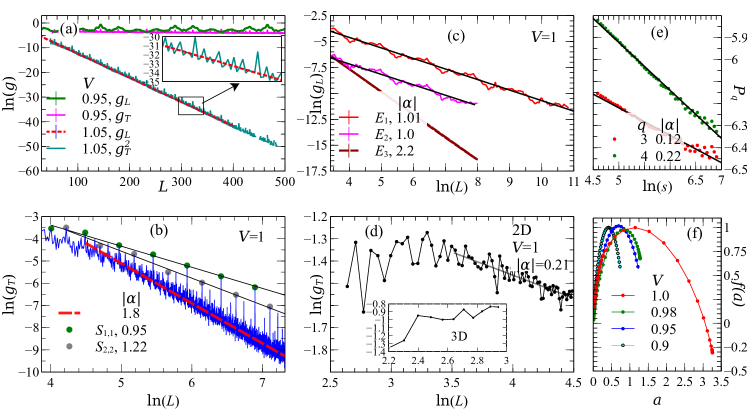
Figure 1: Length-dependent conductances and multifractality in the Auby-Andre model in $1d$ and its $2d$ and $3d$ generalizations. (a) Semilog plots versus $L$ of the conductances $g_{\mathrm{T}}$ (Thouless) and $g_{\mathrm{L}}$ (Landauer) at illustrative values of $V$ in the metallic ($V=0.95$) and insulating ($V=1.05$) regimes in $1d$. On the metallic side, both $g_{\mathrm{T}}$ and $g_{\mathrm{L}}$ show non-monotonic (roughly speaking, small-wavelength) fluctuations about an $L$-independent mean value. On the insulating side, $g_{\mathrm{T}}^{2}\propto g_{\mathrm{L}}$; both $g_{\mathrm{L}}$ and $g_{\mathrm{T}}$ decay exponentially with $L$, the latter only on average because $g_{\mathrm{T}}$ still displays non-monotonic fluctuations (enlarged view in the inset). (b) Log-log plots versus $L$ of the Thouless conductance $g_{\mathrm{T}}$, at the $1d$ critical point $V=1$, showing an average decay (dashed red line) with $g_{\mathrm{T}}\propto L^{\alpha}$ and $\alpha\simeq-1.8$, with hierarchically organized peaks, whose heights also decay as a power of $L$ but with different exponents (for notational simplicity denoted generically by $\alpha$), which depend on $\mathcal{S}_{L_{1},L_{2}}$, the set of peaks at the lengths $L_{i+1}=L_{i}+L_{i-1}$, with the seed lengths $L_{1}$ and $L_{2}$; for the illustrative sets $\mathcal{S}_{1,1}$ (green filled circles) and $\mathcal{S}_{2,2}$ (blue filled circles) we obtain the decay exponents $\simeq-0.95$ and $\simeq-1.22$, respectively. (c) Log-log plots versus $L$ of the Landauer conductance $g_{\mathrm{L}}$, at the $1d$ critical point $V=1$, showing an average decay $g_{\mathrm{L}}\propto L^{\alpha(E)}$, with energy-dependent exponents $\alpha(E)$, shown for the representative energies $E_{1}=0$ ($\alpha(E_{1})\simeq-1.01$), $E_{2}=1.98496$ ($\alpha(E_{2})\simeq-1.0$), and $E_{3}=0.18906032$ ($\alpha(E_{3})\simeq-2.2$; see text); note the non-monotonic fluctuations about these mean-decay lines. (d) This non-monotonicity in log-log plots of $g_{\mathrm{T}}(L)$ versus $L$ persists in $2d$ and $3d$ (inset), as we show by illustrative data at the the metal-insulator critical points; in $2d$, the critical $g_{\mathrm{T}}(L)\sim L^{-0.21}$ exhibits an overall subdiffusive scaling. (e) A fractal analysis of the $L$-dependence of the energy-averaged $g_{\mathrm{T}}$, i.e., $g_{\mathrm{T}}^{\infty}$, versus (see Supplementary Information, Sec.S1.2 and the main text) reveals multifractal scaling of the non-monotonic variations of $g_{\mathrm{T}}(L)$ at the critical point. (f) A plot of the singularity spectrum $f(\alpha)$ versus $\alpha$ corroborates this multifractality (see main text); note that the singularity spectrum narrows on the metallic side $V<1$.

We compute the Thouless, $g_{\mathrm{Th}}(E,L)$, and Landauer, $g_{\mathrm{L}}(E,L)$, conductances, at a given energy $E$, for a hypercube of volume $L^{d}$ ($d=1,2,$ and $3$), as a function of the length $L$ and at zero temperature; we obtain the averages of these conductances by varying $\phi$. We find that even the typical conductances, $g(L)$ (either $g=g_{\mathrm{T}}$ or $g_{\mathrm{L}}$) are strongly non-monotonic function of $L$; this implies that a strict application of single-parameter-scaling theory is untenable, especially in $1d$ and $2d$. This non-monotonicity is present in $3d$ too, but it is weaker than in $2d$ and $1d$. The average $L$ dependence of these conductances, in $1d$ and $2d$, for the localized, critical, and delocalized states, can be characterized by average, smooth curves (denoted generically by $\tilde{g}(L)$); from these smooth curves we can obtain the associated beta functions $\beta(\tilde{g})$ for large system sizes.

In $1d$, these $\beta$ functions show discontinuous jumps as we go from localized [$\beta(\tilde{g})\sim\ln(\tilde{g})$] to ballistic metallic states across the transition at $V=V_{c}=1$; the critical state exhibits sub-diffusive power-law scaling, $\tilde{g}\sim L^{\alpha}$ such that $\beta(\tilde{g})=\alpha<d-2=-1$. This subdiffusive scaling is less clear in $2d$ than in $1d$ because the onset of the scaling regime occurs only above a large, microscopic length scale $\ell$; nevertheless, our calculation of the open-system conductance in $2d$ suggests a similar jump in the $\beta$ function via a sub-diffusive critical state at $V_{c}=1$. Furthermore, instead of ballistic scaling for the conductance in the metallic phase, we find super-diffusive behavior, with a constant $\beta(\tilde{g})$ that lies between $d-2$ and $d-1$.

Our results in $3d$ are consistent with a continuous metal-insulator transition at $V_{c}\simeq 2.2$. We obtain scaling collapse for $g_{\mathrm{L}}(L)$ near the transition, with a correlation-length exponent $\nu\simeq 1.6$, a value that is close to the value of this exponent for the Anderson-localization transition in $3d$ (as found in the recent study of Ref. Devakul and Huse (2017), which used moments of the wave function). Moreover, we obtain a continuous $\beta$ function from this scaling collapse; this suggests that the single-parameter-scaling theory is a good approximation for the $3d$ quasiperiodic system we consider. However, a weak, non-monotonic $L$-dependence of the conductance remains and indicates deviations from strict, single-parameter scaling. We do not find a sharp transport signature of the diffusive-metal-to-ballistic transition at $V\simeq 1/V_{c}$, which we expect from duality Devakul and Huse (2017). Given the system sizes we have been able to use in our study in $3d$, we find that the metallic phase, for $V\ {\raise-2.15277pt\hbox{$\buildrel<\over{\sim}$}}\ 1/V_{c}$, exhibits super-diffusive scaling for $\tilde{g}_{\mathrm{L}}(L)$, with a $V$-dependent exponent $1<\alpha<2$ that approaches the ballistic limit ($\alpha=2$) asymptotically for $V\to 0$.

The non-monotonic variation of the conductance with $L$ is most prominent in $1d$, especially for $g_{\mathrm{T}}(L)$, which exhibits resonant transport peaks for sequences of $L$ that depend on the particular quadratic irrational number we use; e.g., for $b=\Phi$, different sequences of peaks occur at the Fibonacci numbers and their combinations. At the critical point, each one of these sequences exhibits power-law scaling, i.e., $g_{\mathrm{T}}(L)\sim L^{\alpha}$ with the exponent $\alpha$ ranging from the almost-diffusive ($\alpha\simeq-1$) to the sub-diffusive ($\alpha<-1$) values for different sequences. We carry out a fractal analysis Kantelhardt (2008) of the $g_{\mathrm{T}}$ versus $L$ plot to obtain multifractal scaling; we quantify this multifractality of the non-monotonic variations of $g_{\mathrm{T}}$ with $L$ via the singularity spectrum $f(\alpha)$ Kantelhardt (2008). (We use the standard notation $\alpha$ for the crowding index Tel (2014); this should not be confused with the exponent $\alpha$ for the power-law scaling of the conductances.) At the critical point, we find a broad singularity spectrum $f(\alpha)$; this narrows in the metallic phase. Such multifractal scaling of the conductances, as a function of $L$, is a fundamental difference between quasiperiodic and random systems.

We show that $g_{\mathrm{L}}(L)$ also fluctuates with $L$; however, it does not exhibit prominent resonant peaks at distinct sequences of lengths, even in $1d$. Hence, our results indicate a clear distinction between isolated and open-system conductances, as measured through Thouless and Landauer conductances, respectively. Our results reveal very rich transport properties for finite-size quasiperiodic systems; especially in $1d$ and $2d$, these properties are significantly different from their counterparts random systems.

In the next Section we discuss our results in detail. We give some additional aspects of our calculations and numerical computations in the Supplementary Information.

II Results

II.1 Thouless conductance

We first characterize the response of our isolated, finite system to boundary perturbation through the Thouless conductance, $g_{\mathrm{T}}=\delta E/\Delta_{E}$, where $\delta E$ is the geometric mean of the shift of the energy levels, around energy $E$, when we change the boundary conditions from periodic, $\psi(r_{\mu}+L)=\psi(r_{\mu})$, to antiperiodic, $\psi(r_{\mu}+L)=-\psi(r_{\mu})$, Edwards and Thouless (1972); Thouless (1974), in a particular direction $\mu=1,\ldots,d$; $\Delta_{E}$ is the mean level spacing at energy $E$ (see Supplementary Information, Sec.S1.1). In a diffusive metal, $g_{\mathrm{T}}$ can be argued to be the same as the usual Landauer $g_{\mathrm{L}}$ Edwards and Thouless (1972); Thouless (1974); Anderson and Lee (1980) and, in the insulating state, it is expected that $\ln(g_{\mathrm{L}})\propto\ln(g_{\mathrm{T}})$ Braun et al. (1997). However, it should be noted that $g_{\mathrm{T}}$ is a property of a closed, finite system with discrete energy eigenvalues; by contrast, in the usual transport set up, the system is connected to infinite leads and hence it has a continuous spectrum. As we show below for the quasiperiodic system we consider, this makes $g_{\mathrm{T}}(L)$ significantly different from $g_{\mathrm{L}}(L)$.

We obtain the mean $\langle g_{\mathrm{T}}\rangle(E,L)$ or typical conductance $\exp{(\langle\ln{g_{\mathrm{T}}(E,L)}\rangle)}$ at an energy $E$ by computing single-particle energy eigenvalues, for both periodic and antiperiodic boundary conditions, via numerical diagonalization of the Hamiltonian in Eq.(1) or its $d$-dimensional generalizations [Eq.(2), see Methods], without the phase factor in the hopping term. The typical and mean Thouless conductances give similar results in $1d$. The latter, $g_{\mathrm{T}}$ at $E=0$, is plotted versus $L$ for $b=\Phi$ in Figs.1, for insulating and metallic phases [Fig.1(a)] and also at the critical point $V=1$ [Fig.1(b)]. We find strong non-monotonicity of $g_{\mathrm{T}}(L)$. We first characterize its overall $L$ dependence by a smooth least-square-fitting curve $\tilde{g}_{\mathrm{T}}(L)$, which shows ballistic behavior in the metallic phase, i.e., $\tilde{g}_{\mathrm{T}}$ independent of $L$; in contrast, the conductance in the localized phase is well described by $\tilde{g}_{\mathrm{T}}(L)\simeq g_{0}(V)e^{-L/\xi}$ even very close to the transition, $V\ {\raise-2.15277pt\hbox{$\buildrel>\over{\sim}$}}\ V_{c}$; $g_{0}$ denotes conductance at a microscopic length scale $\ell\approx 1$ and varies with $V$. However, the critical state exhibits an overall power-law dependence on $L$, $\tilde{g}_{\mathrm{T}}\sim L^{\alpha}$ [the dashed red line in Fig.1(b)] with $\alpha\simeq-1.8$ up to the maximum system size we have studied ($L=3000$).

The non-monotonicity of the Thouless conductance is clearly manifested in the peak and sub-peak structure of $g_{\mathrm{T}}(L)$, in both the metallic and insulating phases [Fig.1(a)]. These peaks are most striking at the critical point [Fig.1(b)], where we find hierarchically organized peaks, whose heights decay as a power of $L$ but with different exponents (for notational simplicity denoted generically by $\alpha$), which depend on $\mathcal{S}_{L_{1},L_{2}}$, the set of peaks at the lengths $L_{i+1}=L_{i}+L_{i-1}$, with the seed lengths $L_{1}$ and $L_{2}$; for the illustrative sets $\mathcal{S}_{1,1}$ (green filled circles and $L_{i}=F_{i}$, the Fibonacci numbers) and $\mathcal{S}_{2,2}$ (blue filled circles and $L_{i}=2F_{i}$) we obtain the decay exponents $\simeq-0.95$ and $\simeq-1.22$, respectively. We can also identify similar sequences of peaks in the metallic and insulating phases [Fig.1(a)]. The development of a quantitative theory of these peaks and their decay exponents $\alpha_{\mathcal{S}}$ is an important challenge.

Similar resonance peaks have been seen at high- or infinite-temperature open-system transport Purkayastha et al. (2017); Varma et al. (2017); Purkayastha et al. (2018); however, this resonance effect is much more striking in the $g_{\mathrm{T}}$ that we calculate. We find similar resonant peaks for the energy-averaged or infinite-temperature Thouless conductance $g_{\mathrm{T}}^{\infty}$ as well (see Supplementary Information). The existence of sharp resonant peaks in $g_{\mathrm{T}}(L)$, upto arbitrary large lengths, is a special feature of $1d$ and points to markedly distinct transport characteristic of quasiperiodic system compared to random systems in $1d$. We find the the resonant peaks to be present in $2d$ and $3d$, albeit much less prominently than in $1d$, as we show in Fig.1(d) at the metal-insulator transition $V=V_{c}$.

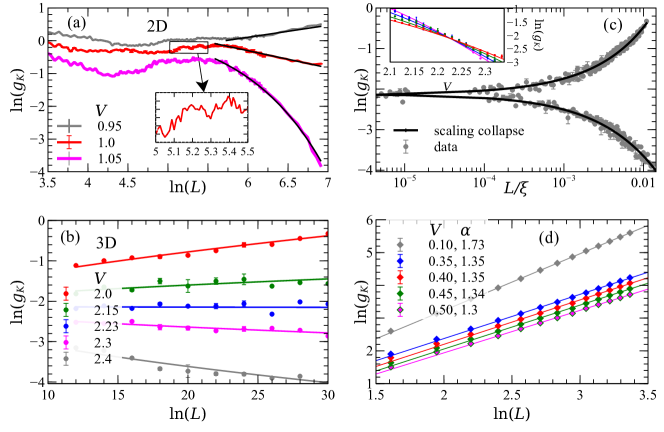
Figure 2: Open-system conductance in $2d$ and $3d$. (a) $g_{\mathrm{K}}(E=0,L)$ for insulating ($V=1.05$), critical ($V=1$) and metallic ($V=1$) states in $2d$. The solid black lines are fitting of the data for the asymptotic $L$ dependence, exponential decay for the insulating state and powerlaw scalings for critical and metallic states. The non-monotonicity of $g_{\mathrm{K}}(L)$ is shown in the inset. (b) Shows $g_{\mathrm{K}}(L)$ across localized to diffusive metal transition in $3d$. A weak non-monotonic variations, larger than the errorbars, can be seen. The solid lines are fit to the data obtained via scaling collapse, shown in (c). The inset in (c) clearly indicates the critical point at $V_{c}=2.22\pm 0.01$ in terms of a crossing of $g_{\mathrm{K}}$ vs. $V$ curves for different $L$. (d) Conductance near $V=1/V_{c}\simeq 0.45$ follows super-diffusive scaling, $g_{\mathrm{K}}\sim L^{\alpha}$ with $1<\alpha<2$, as shown by the fits (solid lines) to the data points and it asymptotically approaches to the ballistic scaling deep in the metallic side, e.g. $\alpha=1.73$ for $V=0.1$ as shown.

Conductance multifractality:

We next ask whether the strong, non-monotonic variations of $g_{\mathrm{T}}$ with $L$ in $1d$ [Fig.1(a),(b)] can be quantified in a broader framework, rather than relying, e.g., on the number-theoretic details for specific choices of the irrational number. Motivated by the multiple power laws in Fig.1(b) for different sequences of $L$, we carry out a fluctuation analysis Kantelhardt (2008) of $g_{\mathrm{T}}$, as function of $L$, by using methods that are used to treat fractal time series (see Supplementary Information). We find the intriguing result thath $g_{\mathrm{T}}(L)$ exhibits multifractal scaling of different moments, as we show for a few moments in 1(e). We also calculate the singularity spectrum Tel (2014); Kantelhardt (2008); Goldberger et al. (2000) of $g_{\mathrm{T}}(L)$ (see Supplementary Information). As shown in Fig.1(f), this singularity spectrum $f(\alpha)$ indicates substantial multifractality at the critical point; it narrows in the metallic phase, but a substantial multifractality still persists there. A meaningful multifractal analysis cannot be performed in the insulating phase because the values of the conductance become exponentially small with $L$. We emphasize that the multifractality of conductance reported here is distinct from usual multifractality of wavefunction or two-point conductance Evers and Mirlin (2008) at the $3d$ Anderson transition for random systems. In the latter, typical and mean conductances are monotonic functions of $L$, and, as a result, the particular multifractality of $g_{\mathrm{T}}(L)$, which we find here for $1d$ quasiperiodic system, would be absent. To this end, we show in the Supplementary Information that the usual multifractality of the critical wavefunction, as in the $3d$ Anderson criticality Evers and Mirlin (2008), is also present for quasiperiodic systems in $1d$ Dominguez et al. (1992); Macé, Nicolas and Jagannathan, Anuradha and Piéchon, Frédéric (2016); Macé, Nicolas and Jagannathan, Anuradha and Kalugin, Pavel and Mosseri, Rémy and Piéchon, Frédéric (2017).

We have not been able to carry out a detailed multifractal analysis of $g_{\mathrm{T}}(L)$ in $d=2,3$ because of the limitations of the system sizes that we can obtain, for the Thouless conductance calculation, which require the numerical diagonalization of large matrices. Moreover, the scales of the non-monotonic variations are much weaker in $2d$ and $3d$, compared to those in $1d$, as is evident from Figs.1(b),(d).

II.2 Open-system conductance

We next study the conductance of open systems, starting with Aubry-Andre chain connected to two semi-infinite leads at both ends. In this case, we compute Landauer or Economou-Soukoulis conductance $g_{\mathrm{L}}(E)=T(E)$ Landauer (1970); Economou and Soukoulis (1981), where $T(E)=4\sin^{2}k/|e^{-ik}\psi(L)-\psi(L-1)|^{2}$, is the transmission coefficient at energy $E=2t\cos{k}$, $t$ being the hopping in the tight-binding leads, and wavefunction amplitudes $\psi(L),~{}\psi(L-1)$ are obtained using standard transfer matrix method (see Supplementary Information). For higher dimensions $d=2,3$, we calculate the open-system conductance $g_{\mathrm{K}}$ using Kubo formula for the system connected with leads using recursive Green function method Lee and Fisher (1981); MacKinnon and Kramer (1983) (see Supplementary Information). The open-system Kubo condactance gives results identical to Landauer conductance Fisher and Lee (1981), as we have verified for $1d$ by calculating both $g_{\mathrm{L}}$ and $g_{\mathrm{K}}$.

One dimension:

The results for $\phi$-averaged typical conductance $\exp{\langle\ln{g_{\mathrm{L}}(E=0,L)}\rangle}$, denoted by $g_{\mathrm{L}}$ for brevity, are plotted in Figs.1(a),(c) across metal-insulator transition in $1d$. The overall length dependence in the metallic and insulating phases are same as that of $g_{\mathrm{T}}(L)$, namely ballistic and localized behaviors with $L$, respectively. However, the transport at the critical point is almost diffusive with $g_{\mathrm{L}}\sim L^{-1.01}$ for $E=0$. Since the $1d$ Aubry-Andre chain has a fractal energy spectra dominated by gaps Simon (1982); Kohmoto et al. (1983); Kohmoto (1983); Ostlund et al. (1983); Ostlund and Pandit (1984), it is hard to track the $L$ dependence for an arbitrary energy as it can move into a gap as $L$ is varied. As a result $g_{\mathrm{L}}(E)$ can cease to show the powerlaw scaling and instead exhibit an exponentially decay with $L$ . However, the nearly diffusive powelaw could be clearly observed till the largest system size ($L=5\times 10^{4}$) studied for $E=0$. For a few other energies the powelaw could be tracked till sufficiently large $L$ as shown in Fig.1(c). Conductance at one of the energies ($E\simeq 0.189$) shows strongly subdiffusive behavior with $\alpha\simeq-2.22$. Since conductances at diffrent energies show a range of scaling from diffusive to subdiffusive, it is possible to obtain a overall subdiffusive conductance scaling at higher temperature that averages over a large energy window, as in the earlier studies Purkayastha et al. (2017); Varma et al. (2017); Purkayastha et al. (2018). To summarize, both $g_{\mathrm{L}}$ and $g_{\mathrm{T}}$ indicate the presence of multiple powelaws, depending on energy and/or the sequence $\mathcal{S}$. Also, we find the relation $g_{\mathrm{L}}\propto g_{\mathrm{T}}^{2}$ Anderson and Lee (1980) to hold in the insulating phase, however, not at the critical point, since $g_{\mathrm{L}}(E=0)$ and $g_{\mathrm{T}}(E=0)$ follow different powelaws with $L$.

As is evident from Figs.1(a),(c) (see also Figs.S3(a)-(d), Supplementary Information), the Landauer conductance in $1d$ also shows strong non-monotonic dependence on $L$, both in the metallic and critical state, even after averaging over sufficiently large number of $\phi$’s (see Methods) and there are peaks and subpeaks as in $g_{\mathrm{T}}$, e.g. the dominant peaks appear at some of the Fibonacci numbers. However, peaks are much weaker and do not appear at all $F_{n}$’s. The weakening, and the absence in some cases, of the conductance peaks in open-system conductance, as opposed to that in $g_{\mathrm{T}}$, indicate that the leads have rather drastic effect on the system in the form of broadening and even washing out the resonances.

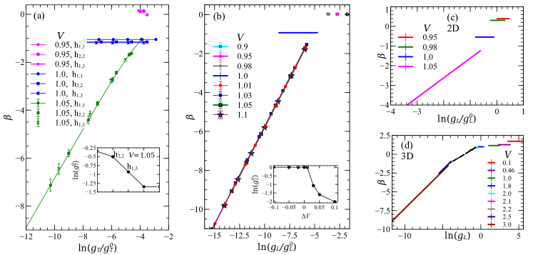
Figure 3: Beta functions in $1d$, $2d$ and $3d$. (a) $\beta(\tilde{g})$ in $1d$ extracted from $\tilde{g}_{\mathrm{T}}$ across metal-insulator transition for various sequences $\mathcal{S}_{L_{1},L_{2}}$, obtained by fitting with exponential decay and power law for $V>1$ and $V\leq 1$, respectively. Same color with different symbols represents $\beta(\tilde{g}_{\mathrm{T}})$ calculated for different $\mathcal{S}$ and the same $V$. On the insulating side to make all the curves fall on the same line we choose different microscopic conductance ($g_{\mathrm{T}}^{0}$) for different sequence (inset). $\beta(\tilde{g})$ extracted in similar manner for (b) $\tilde{g}_{\mathrm{L}}$ in $1d$, (c) $\tilde{g}_{\mathrm{K}}$ in $2d$ and (d) $\tilde{g}_{\mathrm{K}}$ in $3d$ (solid lines) for values of $V$ indicated in the figure panels. In (b) and (c) the straight lines for $\beta(\tilde{g}_{\mathrm{L}})$ in the insulating side ($V>1$) has been collapsed to a single curve by choosing an appropriate $g_{\mathrm{L}}^{0}(V)$, as shown for $1d$ in the inset of (b). In (d) the black dashed line is the $\beta$-function calculated from the scaling collapse of Fig.2(b).

Two dimensions:

The open-system Kubo conductance $g_{\mathrm{K}}(L)$ for $E=0$ in $2d$ is shown in Fig.2(a). Our results for system sizes up to $1000^{2}$ are consistent with a metal-insulator transition at $V=V_{c}=1$, the self-dual point. The conductance in the localized phase, as in $1d$, follows $g_{\mathrm{K}}(L)\simeq g_{0}(V)\exp(-L/\xi)$ for $V>V_{c}$. The metallic phase for $V<V_{c}$ is superdiffusive having $g_{\mathrm{K}}(L)\sim L^{\alpha}$ with $d-2<\alpha\simeq 0.35<d-1$, lying between diffusive and ballistic limits. Here $g_{0}(V)$ is the conductance at a microscopic lenght scale $\ell$. We find the asymptotic scaling behaviors to set in only for $L\gg\ell$, where the microscopic length $\ell(V)$ is substantially large, varying between $L=50-500$ depending on $V$. ballistic increase (not shown in Fig.2(a)), followed by an intermediate regime of length, only above which the scaling regimes ensue. The critical point at $V=V_{c}$ exhibits a subdiffusive length scaling of conductance with $\alpha\simeq-0.52$. Again, strong non-monotonic variations of $g_{\mathrm{K}}(L)$ is observed in all the phases, as demonstrated, e.g., in the inset of Fig.2(a) for the critical state.

Three dimensions:

The results for the $3d$ conductances $g_{\mathrm{K}}(L)$ are shown in Fig.2(b) up to $L=30$ near $V=2.2$. As evident, non-monotonic variations of $g_{\mathrm{K}}(L)$, though present, are drastically reduced for $3d$, in contrast to those in $1d$ and $2d$ [Figs.1(a),(c) and Fig.2(a)]. A critical point at $V=V_{c}\simeq 2.2$ can be clearly detected from the crossing of curves as function of $V$ for different system sizes, as shown in the inset of Fig.2(c). The crossing also indicates a scale invariant conductance at the critical point. A reasonably good scaling collapse of the data using a single-parameter finite-size scaling form $\ln{(g_{\mathrm{K}}(L))}=\mathcal{F}((V_{c}-V)L^{1/\nu})$ could be obtained near the critical point, as shown in Fig.2(c). The finite-size scaling yields $\nu=1.60\pm 0.04$ and $V_{c}=2.22\pm 0.01$, consistent with earlier study in ref.Devakul and Huse (2017) using multifractal finite-size scaling analysis of wave function of closed system. The universal scaling curve describes the $g_{\mathrm{K}}(L,V)$ data quite well as shown by the solid lines in Figs.2(b) and (c)(inset). This is in tune with a continuous metal-insulator transition in $3d$, unlike those in the $1d$ and $2d$ quasiperiodic systems. Moreover, this is consistent with single-parameter scaling law, $\beta(g)=d\ln g/d\ln L$, in the weaker sense Slevin et al. (2001) in the $3d$ quasiperiodic system. However, the persistence of weak non-monotonic system-size variations in the typical conductance still violates the assumption of monotonicity of $\beta(g)$ in the scaling theory Abrahams et al. (1979). The weak non monotonicity, though, could be due to limited system sizes accessed in $3d$ and one might recover strict single-parameter scaling at larger lengths.

From the real space-momentum space duality of the model [(2)], we expect another transition around $V\sim 1/V_{c}\approx 0.45$ from a diffusive to a ballistic phase Devakul and Huse (2017). Our results do not show any transport signature of this transition. As shown in Fig.2(d), $g_{\mathrm{K}}(L)$ around $V=0.45$ can be well described by superdiffusive length scaling with an exponent $\alpha>1$. This could be due to the fact that the duality is not strictly valid for such finite system connected to leads and due to the dichotomy between open and closed system properties, as seen in the $1d$ quasiperiodic system Purkayastha et al. (2017, 2018).

II.3 Beta function

As already remarked, the strong non-monotonicity of even typical $g(L)$ in $1d$ and $2d$ invalidates the application of single-parameter scaling. However, we construct a $\beta(\tilde{g})$, where $\tilde{g}(L)$ is extracted from fitting a smooth curve to the data for $g_{\mathrm{T}}(L)$ and $g_{\mathrm{L}}(L)$, e.g. the ones shown in Fig.1, for several values of $V$ shown in Figs.3(a),(b). This is rather unambiguous procedure in $1d$ where the overall $L$ dependences of conductance in the localized, critical and metallic states are very well described by exponentially localized, subdiffusive and ballistic behaviors, respectively, over several decades of $L$ [Figs.1(a),(c)]. The results for the respective beta functions $\beta(\tilde{g})$ in $1d$ are shown in Figs.3(a),(b) across the metal-insulator transition. In Fig.3(a), $\beta(\tilde{g}_{\mathrm{T}})$ has separate curves for individual phases and the critical point as well as for different sequences. For example, the multiple straight lines at the critical value $V=1$ are due to distinct powerlaws for different sequences shown in Fig.1(b). These, and the jump of beta functions across the critical point clearly violates the assumption of continuity in the single-parameter scaling theory. Similar features are seen in $\beta(\tilde{g}_{\mathrm{L}})$ [Fig.3(b)]. We find $\tilde{g}_{\mathrm{L}}(V,L)=g_{0}(V)\exp(-L/\xi(V))$ to describe quite accurately the conductance in the localized phase, even very close to the transition. However, the coefficient $g_{0}$, a measure of conductance at the microscopic scale $\ell$, varies substantially with $V$ [see inset of Fig.3(b)]. This is unlike, e.g., that in the $1d$ Anderson model where $g_{0}\approx 1$ irrespective of the disorder strength. As a result, one can only obtain a universal $\beta(\tilde{g})$ curve for the localized phase in $1d$ as a function of $\ln(\tilde{g}_{\mathrm{L}}/g_{0}(V))$, i.e. after dividing $g_{\mathrm{L}}$ with appropriate $g_{0}$.

To contrast the above results for beta function for $1d$ quasiperiodic system with that of random system, we show in the Supplementary Information that even a small amount of randomness, introduced, e.g., by elevating the phase $\phi$ to a random variable at each site, makes $g_{\mathrm{L}}(L)$ exponentially decaying with $L$ but with small non-monotonicity and hence leads to a continuous beta function for the overall conductance.

As shown in Fig.3(c), we find very similar result for $\beta(\tilde{g})$ in $2d$, extracted from, e.g., the fitting curves in Fig.2(a). Here the beta function also jumps from a localized behaviour, $\beta(\tilde{g})\propto\ln(\tilde{g}/g_{0})$, to a constant superdiffusive value $\beta(\tilde{g})\simeq 0.3$ in the metallic phase, across a subdiffusive critical state with $\beta(\tilde{g})\simeq-0.52$. However, as commented earlier, the asymptotic scaling behaviors in $2d$ can only be extracted for $L$ above a substantially large microscopic length scale $\ell$ and hence the beta functions are extracted from only a limited ranges of system sizes.

Both the $1d$ and $2d$ results indicate strong violation of the assumption of continuity of $\beta(g)$ in single-parameter scaling theory, even when we disregard the non monotonicity of $g(L)$ by extracting an overall smooth $\tilde{g}(L)$ from the asymptotic behaviors at large system sizes $L$. The above procedure can not be carried out in $3d$ close to the critical point, since our system sizes are limited to much smaller values of $L\leq 30$. However, since the non-monotonicity of $g(L)$ is much weaker in $3d$ and a reasonable scaling collapse of the data could be obtained near the metal-insulator transition, we extract the $\beta(g)$ in Fig.3(d) (dashed black line) near the transition from the scaling fit of $g_{\mathrm{K}}(L)$, shown in Figs.2(b),(c). The fit describes the data well over reasonably large range of $V$ and $L$ and hence suggests the restoration of continuity of $\beta(g)$ for the $3d$ quasiperiodic system, provided we neglect the weak non-monotonic variations of $g(L)$. In Fig.3(d), we also show that the beta function extracted from exponential fit deep in the insulating phase and from powerlaw fits deep in the metallic phase is consistent with that obtained from scaling collapse near the transition.

III Conclusions

In summary, we have studied transport properties in a particular class of self-dual quasiperiodic models in one, two, an three dimensions. We have focussed on the system size dependences of the Thouless and open-system Landauer/Kubo conductances. Our results uncover the intricate nature of transport in quasiperiodic systems, which is manifested in terms of the non-monotonic system-size dependence of typical conductances, e.g., because of transport resonances, and a variety of sub-diffusive power laws for critical transport; these depend on the dimension, energy, and the sequences of length we have described above.

Our results reveal the absence of a single-parameter-scaling description in low dimensions and a recovery of weak single-parameter scaling in $3d$; this has direct implications for universality classes of metal-insulator transition in quasiperiodic systems. We plan to compute the multifractal spectrum of the wavefunction and the Thouless conductance at the critical point in the $3d$ quasiperiodic model and compare it with those at the $3d$ Anderson transition to verify whether they truly belong to the same universality class. It would also be worthwhile to look into generalizations of quasiperiodic systems to other symmetry classes Devakul and Huse (2017) from this perspective. Morover, it would also be interesting to study the implications of sub-diffusive critical states of the non-interacting models, specially in $1d$, on the Griffith-like effect seen experimentally near the MBL transition in interacting quasiperiodic system Lüschen et al. (2017) and incorporate these critical states into a real-space-renormalization-group framework Vosk et al. (2015); Potter et al. (2015); Zhang and Yao (2018) for the MBL transition in quasiperiodic systems.

Appendix A Higher-dimensional generalization of Aubry-Andre model

We study the model proposed in Ref. Devakul and Huse (2017) as a generalization of the self-dual $1d$ Aubry-Andre model to $d$ dimensions, namely,

$$\mathcal{H} =t\sum_{\mathbf{r},\mu}\left(e^{i\phi_{\mu}}c^{\dagger}_{\mathbf{r}+\hat{\mathbf{\mu}}}c_{\mathbf{r}}+\mathrm{h.c}\right)+\sum_{\mathbf{r}}\epsilon_{\mathbf{r}}c^{\dagger}_{\mathbf{r}}c_{\mathbf{r}}$$ (2a)

$$\epsilon_{\mathbf{r}} =2V\sum_{\mu=1}^{d}\cos\left(2\pi\sum_{\nu=1}^{d}B_{\mu\nu}r_{\nu}+\phi_{\mu}\right)$$ (2b)

Where $c_{\mathbf{r}}$ is the fermion operator at site $\mathbf{r}$ of a $d$-dimensional hypercubic lattice and $\mu=1,\dots,d$ denotes Cartesian components. We choose $t=1$, the matrix $\mathbb{B}=b\mathbb{R}$ with $b=\Phi$ and an orthonormal matrix $\mathbb{R}$ Devakul and Huse (2017). In $1d$, $\mathbb{R}=1$ and

$$\mathbb{R} =\begin{bmatrix}c&-s\\ s&c\end{bmatrix}~{}~{}~{}~{}~{}~{}d=2$$ (3a)

$$\mathbb{R} =\begin{bmatrix}c^{2}+s^{3}&cs&cs^{2}-cs\\ cs&-s&c^{2}\\ cs^{2}-cs&c^{2}&c^{2}s+s^{2}\end{bmatrix}~{}~{}~{}~{}~{}~{}d=3$$ (3b)

where $c=\cos\theta$ and $s=\sin\theta$. We choose $\theta=\pi/7$ for all our calculations. For the calculations of conductance of open system connected with leads, we use free boundary condition in transverse directions and hence the phase factor in the hopping term of Eq.(2) can be gauged away. To compare the open system conductance with that of the closed one, we consider the Hamiltonian again without the phase factor in the hopping to calculate the Thouless conductance. We note that for the above transport set up for a finite system the real-momentum space duality of the model Eq.[(2)] Devakul and Huse (2017) is lost. For each finite system with linear dimension $L$ under periodic boundary condition one can generate a self-dual approximation Devakul and Huse (2017). This recipe, however, is not applicable for the transport set up. All the data points for the quasi periodic system, shown here and in the Supplementary Information, are results of averaging over $300-400$ points of $\phi\in[0,2\pi)$ and we checked the convergence of these data for several parameter values with larger number ($\sim 1000-2000$) of $\phi$ averages.

Acknowledgement

We thank Sriram Ganeshan, Shivaji Sondhi, Archak Purakayastha and Chandan Dasgupta for useful discussions. SB acknowledges support from The Infosys Foundation, India. SM acknowledges support from the Indo-Israeli ISF-UGC grant. RP acknowledges support from DST (India).

Appendix S1 Supplementary Information

S1.1 Thouless conductance

The Thouless conductance, discussed in Sec.II.1 of the main text, is defined as

$$\text{g}_{T}(E) =\frac{\delta E}{\Delta_{E}}$$ (S1)

where $\Delta_{E}$ is the mean level spacing and $\delta E$ is the geometric mean of energy level shifts, $|\epsilon_{A}-\epsilon_{P}|$, over an energy window $[E-w,E+w]$ with width $w\gg\Delta_{E}$. Here $\epsilon_{P}$ and $\epsilon_{A}$ are eigenvalues of the Hamiltonian with periodic and anti-periodic boundary conditions, respectively. We calculate the energy spectrum by numerical diagonalization of the quasiperiodic Hamiltonians considered in the main text. The energy spectrum of the Aubry-Andre model has a Cantor set structure with bands of states separated by dense set of gaps Simon (1982); Ostlund and Pandit (1984); Sokoloff (1985). We choose $w$ to be much smaller than the width of the principal bands. Alternatively, $g_{\mathrm{T}}$ can be defined in terms of the mean energy level curvature under a twisted boundary condition or an Aharonov-Bohm flux in a ring geometry Akkermans (1997); Braun et al. (1997). We have checked that $g_{\mathrm{T}}$ obtained from mean energy level curvature gives results similar to that in Eq.(S1). Since the latter does not require the computation of eigenvectors, we have used Eq.(S1) to calculate $g_{\mathrm{T}}$, reported in the main text. We obtain the mean, $\langle g_{\mathrm{T}}\rangle$, and the typical, $\langle\exp{(g_{\mathrm{T}})}\rangle$, conductances by averaging over $\phi$. We also calculate $g_{\mathrm{T}}^{\infty}$, averaged over the whole energy spectrum, as shown in Fig.S1(a) for the critical point ($V=1$) in $1d$. This shows the sharp resonances and various sequences of lengths with different powerlaws, as in Fig.1(b) (main text) for $g_{\mathrm{T}}(E=0)$.

We have also calculated $g_{\mathrm{T}}(L)$ in $1d$ for the irrational number $b=1/\sigma_{s}=\sqrt{2}-1$, the reciprocal of silver ratio. As shown in Fig.S1(b), here also we get similar peaks in the conductance at system sizes related to the Pell numbers, i.e. $P_{n+1}=2P_{n}+P_{n-1}$, with $P_{0}=1$ and $P_{1}=2$, such that $\sigma_{s}=\lim_{n\to\infty}(P_{n+1}/P_{n})$.

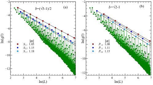
Figure S1: (a) The infinite temperature (i.e. averaged over the full energy spectrum) Thouless conductance ($g^{\infty}_{T}$) for $1d$, with the inverse of golden ratio, $(\sqrt{5}-1)/2$ as the irrational number ($b$) in the potential, is shown varying the system size. $\mathcal{S}$’s are the same sequences described in Fig.1. Conductance for different sequence of system size varies with different exponents $\alpha$, where $g_{\mathrm{T}}\propto L^{\alpha}$. (b) Now the irrational number is changed to the inverse of silver ratio, $(\sqrt{2}-1)$ and $g_{T}^{\infty}$ is calculated. $P_{L_{1},L_{2}}$ represents the sequence of system sizes (related to Pell numbers) started with seeds $L_{1}$ and $L_{2}$ (see S1.1). Both in (a) and (b), the peak of the conductance appears when the system size belongs to the respective sequences.

S1.2 Multifractal Analysis

Motivated by the strong-non monotonicity of $g_{\mathrm{T}}(L)$ in $1d$ [Figs.1(a),(b), main text] and multiple powerlaws in Fig.1(b), we carry out a multifractal fluctuation analysis Kantelhardt (2008); Zhou et al. (2013) of the $g_{\mathrm{T}}(L)$ data, treating it as a time series, i.e. $g_{\mathrm{T}}(i)\equiv g_{\mathrm{T}}(L_{i})$ with $i=1,\dots,N$, where $L_{1}$ and $L_{N}$ are minimum and maximum system sizes studied, respectively. First, we do a cumulative sum of the data, i.e. $y(j)=\sum_{i=1}^{j}g_{\mathrm{T}}(i)$ for $j=1,\dots,N$. Then, to remove any trend from the data, we subtract moving average from each data point. The moving average $\bar{y}(j)$ is the average of $y(j)$’s over an interval (here we used $[j-13,j+13]$) around $j$. This gives us the residual sequence $\tilde{y}(j)=y(j)-\bar{y}(j)$. Now the residual sequence is divide into non-overlapping segments $j_{s}=1,\dots,N_{s}$ of width $s$, where $N_{s}$ is the largest integer not larger than $N/s-1$. The root mean square (rms) fluctuation is calculated for each segment, i.e.

$$F_{s}(j_{s}) =\sqrt{\frac{1}{s}\sum_{j\in j_{s}}\bar{y}^{2}(j)}$$ (S2a)

and various moments, i.e.

$$P_{q} =\left(\frac{1}{N_{s}}\sum_{j_{s}=1}^{N_{s}}F_{s}^{q}(j_{s})\right)^{1/q}$$ (S2b)

are calculated. These moments follow multifractal powelaw scalings with the segments length $s$, i.e. $P_{q}(s)\sim s^{h(q)}$, as shown for $q=3,4$ in Fig.1(e) (main text) at the $1d$ critical point.

To quantify the multifractality, we can obtain the singularity spectrum through a Legendre transform, $f(\alpha)=q[\alpha-h(q)]+1$, with $\alpha=\partial[qh(q)-1]/\partial q$. For a more refined multifractal analysis, we use a wavelet transform the Thouless conductance data, namely we convolve the data set with a fixed order derivative of the Gaussian funtion, ${G}^{n}(x)=d^{n}(e^{-x^{2}/2})/dx^{n}$. This removes any polynomial trend in the data upto order $n-1$ leaving only the singular dependence. Now this power can be extracted via a log-log fitting and thus, the singularity spectrum can be obtained. To this end, we use the codes of ref.Goldberger et al. (2000). In our calculation we use the fourth order derivative of Gaussian function. The resulting singularity spectra $f(\alpha)$ for $1d$ Thouless conductance in the metallic phase and at the critical point are shown in Fig.1(f). The singularity spectra computed using moments in Eqs.S2 are qualitatively similar to that obtained via wavelet transform method.

S1.2.1 Wavefunction Multifractality

The conductance multifractality obtained in the preceding section from the $L$ dependence of Thouless conductance directly characterizes the violation of the assumption of monotonicity in single-parameter scaling theory. As discussed in the main text, this kind of multifractality in quasiperiodic system is quite different from well-known the wavefunction multifractality at the critical point between metal and insulator in random system, e.g. at the 3d Anderson transition Evers and Mirlin (2008). Conventionally, the multifractality of critical single-particle eigenstates $\psi_{r}$ is analyzed in terms of the moments of wavefunction amplitude Evers and Mirlin (2008), i.e. $P^{\psi}_{q}=\sum_{r}|\psi_{r}|^{2q}$, which upon disorder averaging follows a powerlaw scaling $\langle P_{q}\rangle\sim L^{-\tau(q)}$, with an exponent $\tau(q)=d(q-1)+\Delta_{q}$ non-trivially dependent on $q$, as characterized by the anomalous dimension $\Delta(q)$. We show in Fig.S2 that, much like at the $3d$ Anderson criticality Evers and Mirlin (2008), the critiacal wavefunctions of quasiperiodic system also possess the usual multifractality in $1d$ as characterized by the singularity spectrum obtained from the Legendre transform of $\tau(q)$ Dominguez et al. (1992).

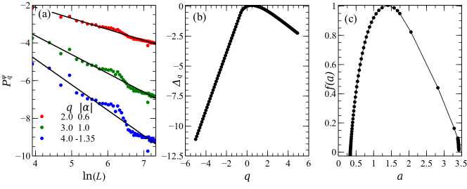
Figure S2: (a) The scaling of different moments of the wave function of the 1D Hamiltonian, $P_{q}^{\psi}\sim L^{-\alpha}$, averaged over all energy, is shown here. (b) Shows the anomalous dimension. (c) The singularity spectrum shows the multifractal nature.

S1.3 Landauer conductance in $1d$

Schrodinger equation for the $1d$ Hamiltonian, given in Eq.(1), can be written in the latttice basis, $\{\psi_{r}\}$ in the following way

$$\left({\begin{array}[]{c}\psi_{r+1}\\ \psi_{r}\\ \end{array}}\right)=\left({\begin{array}[]{cc}\epsilon_{r}&-1\\ 1&0\\ \end{array}}\right)\left({\begin{array}[]{c}\psi_{r}\\ \psi_{r-1}\\ \end{array}}\right)=M_{r}\left({\begin{array}[]{c}\psi_{r}\\ \psi_{r-1}\\ \end{array}}\right)=\prod_{i=1}^{r}M_{i}\left({\begin{array}[]{c}\psi_{1}\\ \psi_{0}\\ \end{array}}\right)=\textbf{M}\left({\begin{array}[]{c}\psi_{1}\\ \psi_{0}\\ \end{array}}\right),$$ (S3)

where $\epsilon_{r}=E-2V\cos(2\pi br+\phi)$ and $E$ is the energy of interest. Iterating this equation we can calculate the amplitude at the end points given the two starting amplitudes. This transfer matrix M is related to the transmission matrix T via a transformation Markos (2006),

$$\textbf{T}=\textbf{Q}^{-1}\textbf{MQ},$$ (S4)

where

$$\textbf{Q}=\left({\begin{array}[]{cc}1&1\\ e^{-ik}&e^{ik}\\ \end{array}}\right).$$ (S5)

Here the disordered region is considered to exist for $N>i>0$ and $V=0$ at all other points, with transmitted wave amplitude $\psi_{-1}=e^{ik}$ and $\psi_{0}=1$ for a wave propagating from $i>N$ region to $i<0$. The Landauer conductance is given by

$$g_{\mathrm{L}}=\dfrac{|t|^{2}}{|r|^{2}},$$ (S6)

where $t$ and $r$ is the transmission and reflection amplitude in the transmission matrix. The Landauer conductance $g_{\mathrm{L}}(L)$ is shown in Figs.S3(a)-(d) for metallic and critical states. The strong non-monotonicty in $g_{\mathrm{L}}(L)$ is evident.

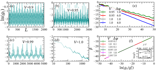
Figure S3: (b)-(e) have the same axes labeling as (a). (a)-(d) $g_{\mathrm{L}}(L)$ for $1d$, both in metallic side and at the critical point, are shown. (e) In the presence of randomly chosen phase at each site, from a uniform random disorder $[-\Delta\phi/2,\Delta\phi/2]$, the system becomes insulator for any nonzero value of $V$ and $\Delta\phi$, which indicates the perturbation to be relevant.For a weak phase disorder the monotonicity of $g_{\mathrm{L}}(L)$ is still present. The data points are averaged over $3000$ disorder realization. (f) Ignoring the $L$ dependent fluctuation in weak disorder a continuous $\beta$ function is obtained, hence the single-parameter scaling theory is recovered for the large length scale behavior of the conductance.

S1.4 Kubo conductance

The open-system (dimensionless) conductance at energy $E$ for the system described by the quasiperiodic Hamiltonians [Eqs.(1),(2)] connected with non-interacting leads at the two ends along $x$ direction is given by the Kubo formula Fisher and Lee (1981); Lee and Fisher (1981),

$$g_{\mathrm{K}}(E)=2\text{Tr}[\hat{I}^{x}(x)\hat{G}^{\prime\prime}(E)\hat{I}^{x}(x^{\prime})\hat{G}^{\prime\prime}(E)].$$ (S7)

Where $G"=(1/2i)(G^{-}-G^{+})$ is obtained in terms of the Green’s functions $G^{\pm}(E)=(E-H\pm i\eta)^{-1}$, $H$ being the Hamiltonian of the whole system including the leads. The current operator is

$$\hat{I}(j)=it\sum_{l}({|j-1,l\rangle}{\langle j,l|}-{|j,l\rangle}{\langle j-1,l|})$$ (S8)

$l$ is the index to represent sites on any slice $j$ perpendicular to the direction $x$. The conductance then simplifies to

$$g_{\mathrm{K}}=2\text{Tr}[2G^{\prime\prime}(j,j)G^{\prime\prime}(j-1,j-1)-G^{\prime\prime}(j-1,j)^{2}-G^{\prime\prime}(j,j-1)^{2}].$$ (S9)

The trace is over $l$ i.e in the transverse direction. We evaluate the conductance by calculating the Green’s functions in Eq.(S9) via the standard recursive Green’s function method described in refs.Lee and Fisher (1981); MacKinnon and Kramer (1983); Verges (1999). The attached leads have same width as that of the system and we use hard-wall or open boundary condition in the transverse directions.

S1.5 Beta function calculations

To extract the beta functions in Figs.3 (main text), we carry out linear fitting for the $\ln{g}$ vs. $\ln{L}$ curves in the region $V\leq 1$ and, for $V>1$, we do the same for $\ln{g}$ vs. $L$ curves. This gives a powerlaw dependency of conductance on $L$ for metallic phase ($V\leq 1$) and exponential dependency in the insulating regime ($V>1$). The scaling-theory beta function $\beta(g)=d\ln{g}/d\ln{L}$ is calculated by taking logarithmic derivative of the fitting curves. In $3d$, close to the critical point. we perform a scaling collapse of the data following ref.Slevin et al. (2001). To this end, we assume a single-parameter finite-size scaling form for the conductance, namely

$$\ln{g}=\mathcal{F}(\Psi L^{1/\nu})$$ (S10)

The relevant scaling variable $\Psi$, in terms of dimensionless parameter $v=(V-V_{c})/V_{c}$, is approximated as $\Psi=\Psi_{1}v+\Psi_{2}v^{2}$ and expand the scaling function $\mathcal{F}$ upto third-order polynomial. We minimize the quantity $\sum_{i}(\ln{g_{i}}-\mathcal{F}(\Psi_{i}L_{i}^{1/\nu}))^{2}$ to obtain the fitting parameters, $V_{c}$, $\nu$, $\Psi_{1}$, $\Psi_{2}$ and the coefficients of the third-order polynomial, where index $i$ represents each point of the data set $\{V,L\}$. Once the scaling function $\mathcal{F}(x)$ is known in terms of these parameters, we calculate the smooth $\beta$ function in $3d$ near the metal-insulator transition at $V_{c}\simeq 2.2$, as shown in Fig.2(d).

S1.5.1 Effects of phase disorder

In Fig.S3(f), the results for $\beta(\tilde{g}_{\mathrm{L}})$ is shown for a $1d$ model where we modify the quasiperiodic potential in Eq.(1) from $\cos(2\pi br+\phi)$ to $\cos(2\pi br+\phi_{r})$ with $\phi_{r}$ an uncorrelated random phase at each site chosen uniformly from $[-\Delta\phi/2,\Delta\phi/2]$. The phase randomness, even if weak, leads to localization, as eveident from exponential decay of conductance with $L$ in Fig.S3(e), even for $V<1$. As expected for a random system, one gets back a continuous beta function, considering the conductance dependence on long window of system sizes, i.e. ignoring the non-monotonicity with $L$ at small lengths, for weak strength of the randomness, in contrast to that in Fig.3(b). As shown in Fig.S3(e), the bare $g_{\mathrm{L}}(L)$ has a non-monotonic behavior with $L$ in the presence of weak phase randomness, but the non monotonicity goes away as the randomness increases, completely restoring single parameter scaling theory even for moderate strength of disorder.

References

- Abrahams et al. (1979) E. Abrahams, P. W. Anderson, D. C. Licciardello, and T. V. Ramakrishnan, “Scaling theory of localization: Absence of quantum diffusion in two dimensions,” Phys. Rev. Lett. 42, 673–676 (1979).
- Anderson (1958) P. W. Anderson, “Absence of diffusion in certain random lattices,” Phys. Rev. 109, 1492–1505 (1958).
- Aubry and Andre (1980) S. Aubry and G. Andre, “Analyticity breaking and anderson localization in incommensurate lattices,” Ann. Israel Phys. Soc. 3, 18 (1980).
- Simon (1982) Barry Simon, “Almost periodic Schrödinger operators: A Review,” Advances in Applied Mathematics 3, 463 – 490 (1982).
- Sokoloff and José (1982) J. B. Sokoloff and Jorge V. José, “Localization in an almost periodically modulated array of potential barriers,” Phys. Rev. Lett. 49, 334–337 (1982).
- Thouless and Niu (1983) D. J. Thouless and Q. Niu, “Wavefunction scaling in a quasi-periodic potential,” Journal of Physics A: Mathematical and General 16, 1911 (1983).
- Kohmoto et al. (1983) M. Kohmoto, L. P. Kadanoff, and C. Tang, “Localization problem in one dimension: Mapping and escape,” Phys. Rev. Lett. 50, 1870–1872 (1983).
- Kohmoto (1983) M. Kohmoto, “Metal-insulator transition and scaling for incommensurate systems,” Phys. Rev. Lett. 51, 1198–1201 (1983).
- Ostlund et al. (1983) S. Ostlund, R. Pandit, D. Rand, H. J. Schellnhuber, and E. D. Siggia, “One-Dimensional Schrödinger Equation with an Almost Periodic Potential,” Phys. Rev. Lett. 50, 1873–1876 (1983).
- Ostlund and Pandit (1984) S. Ostlund and R. Pandit, “Renormalization-group analysis of the discrete quasiperiodic Schrödinger equation,” Phys. Rev. B 29, 1394–1414 (1984).
- Sokoloff (1985) J. B.• Sokoloff, “Unusual band structure, wave functions and electrical conductance in crystals with incommensurate periodic potentials,” Physics Reports 126, 189 – 244 (1985).
- Schreiber et al. (2015) M. Schreiber, S. S. Hodgman, P. Bordia, H. P. Lüschen, M. H. Fischer, R. Vosk, E. Altman, U. Schneider, and I. Bloch, “Observation of many-body localization of interacting fermions in a quasirandom optical lattice,” Science 349, 842–845 (2015).
- Purkayastha et al. (2017) A. Purkayastha, A. Dhar, and M. Kulkarni, “Nonequilibrium phase diagram of a one-dimensional quasiperiodic system with a single-particle mobility edge,” Phys. Rev. B 96, 180204 (2017).
- Purkayastha et al. (2018) A. Purkayastha, S. Sanyal, A. Dhar, and M. Kulkarni, “Anomalous transport in the Aubry-André-Harper model in isolated and open systems,” Phys. Rev. B 97, 174206 (2018).
- Varma et al. (2017) V. K. Varma, C. de Mulatier, and M. Žnidarič, “Fractality in nonequilibrium steady states of quasiperiodic systems,” Phys. Rev. E 96, 032130 (2017).
- Khemani et al. (2017) V. Khemani, D. N. Sheng, and D. A. Huse, “Two universality classes for the many-body localization transition,” Phys. Rev. Lett. 119, 075702 (2017).
- De Roeck and Huveneers (2017) Wojciech De Roeck and Fran çois Huveneers, “Stability and instability towards delocalization in many-body localization systems,” Phys. Rev. B 95, 155129 (2017).
- Potirniche et al. (2018) I.-D. Potirniche, S. Banerjee, and E. Altman, “On the stability of many-body localization in ,” ArXiv e-prints (2018), arXiv:1805.01475 [cond-mat.dis-nn] .
- Evers and Mirlin (2008) F. Evers and A. D. Mirlin, “Anderson transitions,” Rev. Mod. Phys. 80, 1355–1417 (2008).
- Anderson et al. (1980) P. W. Anderson, D. J. Thouless, E. Abrahams, and D. S. Fisher, “New method for a scaling theory of localization,” Phys. Rev. B 22, 3519–3526 (1980).
- Altshuler (1985) B. L. Altshuler, “Fluctuations in the extrinsic conductivity of disordered conductors,” JETP Lett. 41, 648 (1985).
- Lee and Stone (1985) P. A. Lee and A. D. Stone, “Universal conductance fluctuations in metals,” Phys. Rev. Lett. 55, 1622–1625 (1985).
- Lee and Fisher (1981) P. A. Lee and D. S. Fisher, “Anderson localization in two dimensions,” Phys. Rev. Lett. 47, 882–885 (1981).
- Pichard and Sarma (1981) J. L. Pichard and G. Sarma, “Finite-size scaling approach to anderson localisation. ii. quantitative analysis and new results,” Journal of Physics C: Solid State Physics 14, L617 (1981).
- MacKinnon and Kramer (1983) A. MacKinnon and B. Kramer, “The scaling theory of electrons in disordered solids: Additional numerical results,” Zeitschrift für Physik B Condensed Matter 53, 1–13 (1983).
- Slevin et al. (2001) K. Slevin, P. Markoš, and T. Ohtsuki, “Reconciling conductance fluctuations and the scaling theory of localization,” Phys. Rev. Lett. 86, 3594–3597 (2001).
- Devakul and Huse (2017) T. Devakul and D. A. Huse, “Anderson localization transitions with and without random potentials,” Phys. Rev. B 96, 214201 (2017).
- Deng et al. (2017) D.-L. Deng, S. Ganeshan, X. Li, R. Modak, S. Mukerjee, and J. H. Pixley, “Many-body localization in incommensurate models with a mobility edge,” Annalen der Physik 529, 1600399 (2017).
- Ganeshan et al. (2015) S. Ganeshan, J. H. Pixley, and S. Das Sarma, “Nearest neighbor tight binding models with an exact mobility edge in one dimension,” Phys. Rev. Lett. 114, 146601 (2015).
- Kantelhardt (2008) J. W. Kantelhardt, “Fractal and Multifractal Time Series,” ArXiv e-prints (2008), arXiv:0804.0747 [physics.data-an] .
- Tel (2014) T. Tel, “Fractals, multifractals, and thermodynamics,” Zeitschrift fur Naturforschung A 43, 1154–1174 (2014).
- Edwards and Thouless (1972) J. T. Edwards and D. J. Thouless, “Numerical studies of localization in disordered systems,” Journal of Physics C: Solid State Physics 5, 807 (1972).
- Thouless (1974) D. J. Thouless, “Electrons in disordered systems and the theory of localization,” Physics Reports 13, 93 – 142 (1974).
- Anderson and Lee (1980) P. W. Anderson and P. A. Lee, “The thouless conjecture for a one-dimensional chain,” Progress of Theoretical Physics Supplement 69, 212–219 (1980).
- Braun et al. (1997) D. Braun, E. Hofstetter, A. MacKinnon, and G. Montambaux, “Level curvatures and conductances: A numerical study of the thouless relation,” Phys. Rev. B 55, 7557–7564 (1997).
- Goldberger et al. (2000) A. L. Goldberger, L. A. N. Amaral, L. Glass, J. M. Hausdorff, P. Ch. Ivanov, R. G. Mark, J. E. Mietus, G. B. Moody, C.-K. Peng, and H. E. Stanley, “PhysioBank, PhysioToolkit, and PhysioNet: Components of a New Research Resource for Complex Physiologic Signals,” Circulation 101, e215– e220 (2000).
- Dominguez et al. (1992) D. Dominguez, C. Wiecko, and J. V. Jose, “Wave-function and resistance scaling for quadratic irrationals in Harper’s equation,” Phys. Rev. B 45, 13919 (1992).
- Macé, Nicolas and Jagannathan, Anuradha and Piéchon, Frédéric (2016) Macé, Nicolas and Jagannathan, Anuradha and Piéchon, Frédéric, “Fractal dimensions of wave functions and local spectral measures on the fibonacci chain,” Phys. Rev. B 93, 205153 (2016).
- Macé, Nicolas and Jagannathan, Anuradha and Kalugin, Pavel and Mosseri, Rémy and Piéchon, Frédéric (2017) Macé, Nicolas and Jagannathan, Anuradha and Kalugin, Pavel and Mosseri, Rémy and Piéchon, Frédéric, “Critical eigenstates and their properties in one- and two-dimensional quasicrystals,” Phys. Rev. B 96, 045138 (2017).
- Landauer (1970) R. Landauer, “Electrical resistance of disordered one-dimensional lattices,” The Philosophical Magazine: A Journal of Theoretical Experimental and Applied Physics 21, 863–867 (1970).
- Economou and Soukoulis (1981) E. N. Economou and C. M. Soukoulis, “Static conductance and scaling theory of localization in one dimension,” Phys. Rev. Lett. 46, 618–621 (1981).
- Fisher and Lee (1981) D. S. Fisher and P. A. Lee, “Relation between conductivity and transmission matrix,” Phys. Rev. B 23, 6851–6854 (1981).
- Lüschen et al. (2017) H. P. Lüschen, P. Bordia, S. Scherg, F. Alet, E. Altman, U. Schneider, and I. Bloch, “Observation of slow dynamics near the many-body localization transition in one-dimensional quasiperiodic systems,” Phys. Rev. Lett. 119, 260401 (2017).
- Vosk et al. (2015) R. Vosk, D. A. Huse, and E. Altman, “Theory of the many-body localization transition in one-dimensional systems,” Phys. Rev. X 5, 031032 (2015).
- Potter et al. (2015) A. C. Potter, R. Vasseur, and S. A. Parameswaran, “Universal properties of many-body delocalization transitions,” Phys. Rev. X 5, 031033 (2015).
- Zhang and Yao (2018) S.-X. Zhang and H. Yao, “Universal properties of many-body localization transitions in quasiperiodic systems,” ArXiv e-prints (2018), arXiv:1805.05958 [cond-mat.str-el] .
- Akkermans (1997) E. Akkermans, “Twisted boundary conditions and transport in disordered systems,” Journal of Mathematical Physics 38, 1781–1793 (1997).
- Zhou et al. (2013) W. Zhou, Y. Dang, and Gu R., “Efficiency and multifractality analysis of CSI 300 based on multifractal detrending moving average algorithm,” Physica A 392, 1429–1438 (2013).
- Markos (2006) P. Markos, “Numerical Analysis of The Anderson Localization,” Acta Physica Slovaca 56, 561–686 (2006).
- Verges (1999) J. A. Verges, “Computational implementation of the Kubo formula for the static conductance: application to two-dimensional quantum dots,” Computer Physics Communications 118, 71–80 (1999).