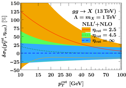
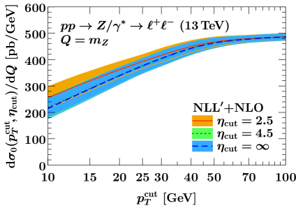
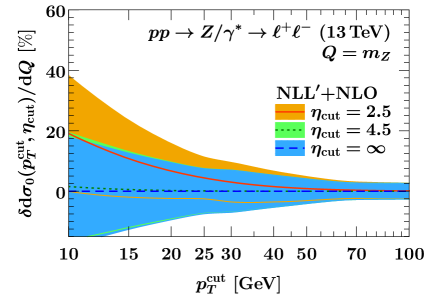
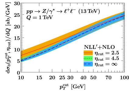
Jet Veto Resummation with Jet Rapidity Cuts

Johannes K. L. Michel    Piotr Pietrulewicz    and Frank J. Tackmann
(October 30, 2018)
Abstract

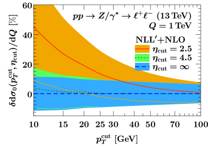
Jet vetoes are widely used in experimental analyses at the LHC to distinguish different hard-interaction processes. Experimental jet selections require a cut on the (pseudo)rapidity of reconstructed jets, |ηjet|ηcutsubscript𝜂jetsubscript𝜂cut|\eta_{\rm jet}|\leq\eta_{\rm cut}. We extend the standard jet-pTsubscript𝑝𝑇p_{T} (jet-veto) resummation, which implicitly works in the limit ηcutsubscript𝜂cut\eta_{\rm cut}\to\infty, by incorporating a finite jet rapidity cut. We also consider the case of a step in the required pTcutsuperscriptsubscript𝑝𝑇cutp_{T}^{\rm cut} at an intermediate value of |η|2.5similar-to-or-equals𝜂2.5|\eta|\simeq 2.5, which is of experimental relevance to avoid the increased pile-up contamination beyond the reach of the tracking detectors. We identify all relevant parametric regimes, discuss their factorization and resummation as well as the relations between them, and show that the phenomenologically relevant regimes are free of large nonglobal logarithms. The ηcutsubscript𝜂cut\eta_{\rm cut} dependence of all resummation ingredients is computed to the same order to which they are currently known for ηcutsubscript𝜂cut\eta_{\rm cut}\to\infty. Our results pave the way for carrying out the jet-veto resummation including a sharp cut or a step at ηcutsubscript𝜂cut\eta_{\rm cut} to the same order as is currently available in the ηcutsubscript𝜂cut\eta_{\rm cut}\to\infty limit. The numerical impact of the jet rapidity cut is illustrated for benchmark qq¯𝑞¯𝑞q\bar{q} and gg𝑔𝑔gg initiated color-singlet processes at NLL+{}^{\prime}+NLO. We find that a rapidity cut at high ηcut=4.5subscript𝜂cut4.5\eta_{\rm cut}=4.5 is safe to use and has little effect on the cross section. A sharp cut at ηcut=2.5subscript𝜂cut2.5\eta_{\rm cut}=2.5 can in some cases lead to a substantial increase in the perturbative uncertainties, which can be mitigated by instead using a step in the veto.

1 Introduction

Measurements that involve a veto on additional jets, or more generally that divide events into exclusive jet bins, play an important role at the LHC, e.g. in Higgs and diboson measurements or in searches for physics beyond the Standard Model. The jet binning differentiates between hard processes that differ in the number of hard signal jets, and hence allows one to separate signal and background processes. The separation into 00-jet and 1absent1\geq 1-jet bins also provides a model-independent way to discriminate between qq¯𝑞¯𝑞q\bar{q} and gg𝑔𝑔gg initiated processes [1].

A veto on jets with transverse momentum pT>pTcutsubscript𝑝𝑇superscriptsubscript𝑝𝑇cutp_{T}>p_{T}^{\rm cut} gives rise to double logarithms ln2(pTcut/Q)superscript2superscriptsubscript𝑝𝑇cut𝑄\ln^{2}(p_{T}^{\rm cut}/Q) at each order in αssubscript𝛼𝑠\alpha_{s}, where Q𝑄Q is the characteristic momentum transfer of the hard interaction. These logarithms dominate the perturbative series when pTcutQmuch-less-thansuperscriptsubscript𝑝𝑇cut𝑄p_{T}^{\rm cut}\ll Q, and represent an important source of theory uncertainty [2, 3]. They can be systematically resummed to improve the perturbative predictions and assess the associated uncertainties, which has been well-developed in Drell-Yan and Higgs production [4, 5, 2, 6, 7, 8, 9, 10, 11, 12, 13, 14, 15, 16, 17], and has also been applied to several other color-singlet processes [18, 19, 20, 21, 22, 23, 24, 1, 25].
Refer to caption
Refer to caption
Refer to caption
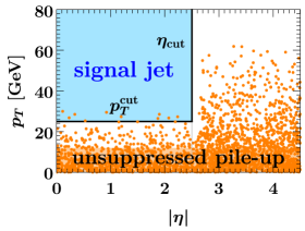
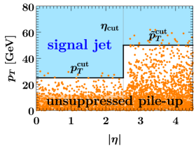
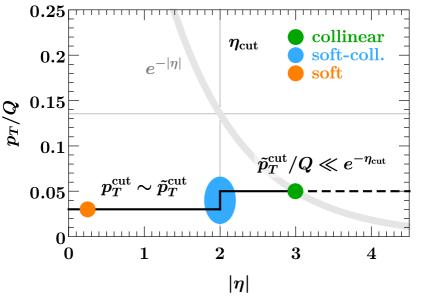
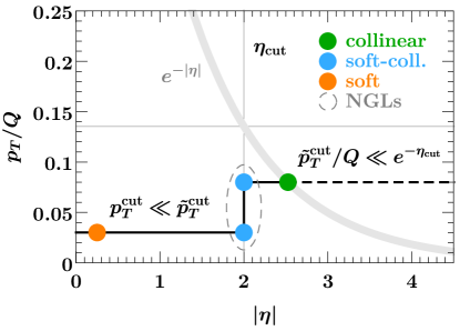
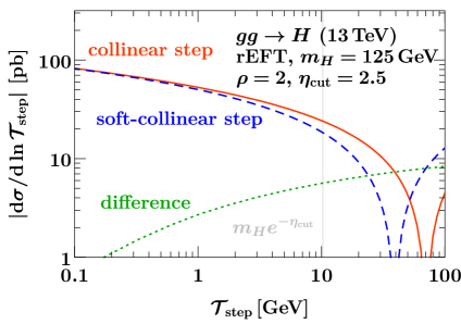
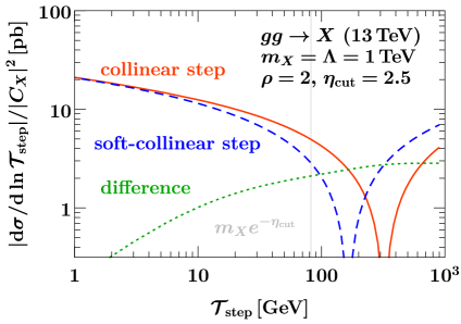
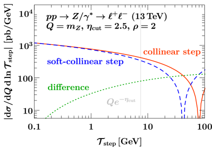
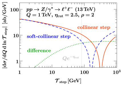
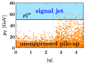
Figure -1139: Cartoon of possible strategies to avoid contamination from unsuppressed pile up in jet-binned analyses. The pile-up suppression is much better in the pseudorapidity range |η|2.5less-than-or-similar-to𝜂2.5\lvert\eta\rvert\lesssim 2.5, where it can use information from the tracking detectors. To avoid the higher pile-up contamination in the forward region, one can raise the jet threshold (left panel), only consider central jets (middle panel), or combine both approaches by using a step-like jet selection (right panel).

Experiments can only reconstruct jets up to some maximal pseudorapidity |η|ηcut𝜂subscript𝜂cut\lvert\eta\rvert\leq\eta_{\rm cut} due to the range of the detector, e.g. for ATLAS and CMS ηcut4.5similar-tosubscript𝜂cut4.5\eta_{\rm cut}\sim 4.5. In principle, the utility of the jet binning to discriminate between different hard processes increases for a tighter jet veto (smaller pTcutsuperscriptsubscript𝑝𝑇cutp_{T}^{\rm cut}). However, jets with small transverse momenta are difficult to reconstruct experimentally, especially for pseudorapidity |η|2.5greater-than-or-equivalent-to𝜂2.5\lvert\eta\rvert\gtrsim 2.5 beyond the reach of the tracking detectors, which are important to suppress the large contamination from pile up (e.g. in the jet vertex tagging algorithm used by ATLAS [26]). This is illustrated in figure -1139. As the LHC luminosity increases and pile-up conditions become harsher, the contamination from unsuppressed pile-up jets grows worse and must be avoided. One option is to increase the overall pTcutsuperscriptsubscript𝑝𝑇cutp_{T}^{\rm cut}. For example, in the context of Higgs measurements, the increased pile up in Run 2 has forced raising the jet threshold from 25GeV25GeV25\,\mathrm{GeV} to 30GeV30GeV30\,\mathrm{GeV}. This however weakens the jet veto and thus reduces its utility. Alternatively, to avoid raising the jet threshold, one can consider jets only in a restricted pseudorapidity range of |η|2.5less-than-or-similar-to𝜂2.5\lvert\eta\rvert\lesssim 2.5. However, this looses the discrimination power from forward jets, which are a distinguishing feature of some processes (most notably weak-boson fusion topologies in Higgs and diboson production). The best possible option combines both approaches and performs a step-like jet selection, with a lower pTcutsuperscriptsubscript𝑝𝑇cutp_{T}^{\rm cut} threshold for central jets and a somewhat higher p~Tcutsuperscriptsubscript~𝑝𝑇cut\tilde{p}_{T}^{\rm cut} threshold for forward jets. For example, recent ATLAS Higgs measurements [27] reconstruct jets using pTcut=25GeVsuperscriptsubscript𝑝𝑇cut25GeVp_{T}^{\rm cut}=25\,\mathrm{GeV} for |η|<2.4𝜂2.4\lvert\eta\rvert<2.4 and p~Tcut=30GeVsuperscriptsubscript~𝑝𝑇cut30GeV\tilde{p}_{T}^{\rm cut}=30\,\mathrm{GeV} for |η|>2.4𝜂2.4\lvert\eta\rvert>2.4 (and no jets beyond rapidity |y|=4.4𝑦4.4\lvert y\rvert=4.4).

A discontinuous step in the jet threshold can also pose challenges on its own, as it makes the experimental measurements more complex. Theoretically, we will see that it can complicate the resummation of logarithms in some extreme cases. An alternative to a step is to use jet vetoes that smoothly depend on the jet rapidity [16, 28], providing a tighter veto at central rapidities and a looser one at forward rapidities. These rapidity-dependent vetoes can also be supplemented with an additional sharp jet rapidity cut, which we briefly discuss in appendix B.

The usual jet-pTsubscript𝑝𝑇p_{T} resummations [6, 7, 8, 9, 12, 13] do not account for any jet rapidity dependence, i.e., the resummation is performed for ηcutsubscript𝜂cut\eta_{\rm cut}\to\infty. Using parton-shower Monte Carlos, one finds that a jet rapidity cut at ηcut=4.5subscript𝜂cut4.5\eta_{\rm cut}=4.5 has a very small numerical effect, while ηcut=2.5subscript𝜂cut2.5\eta_{\rm cut}=2.5 has a sizable effect on the jet-pTsubscript𝑝𝑇p_{T} spectrum in Higgs production (see e.g. refs. [2, 6]), so it is important to properly include it in the resummation. This was already pointed out in ref. [8], where it was also speculated that a jet rapidity cut might change the resummation structure.

Our analysis in this paper fully addresses these questions by systematically incorporating the jet rapidity cut into the jet-pTsubscript𝑝𝑇p_{T} resummation, including in particular the case of a step-like veto. For this purpose, we extend the formalism of refs. [8, 13], which uses the framework of Soft-Collinear Effective Theory (SCET) [29, 30, 31, 32]. To be concrete, our discussion focuses on color-singlet production, including the important cases of Higgs and Drell-Yan production. Our results for how to incorporate the ηcutsubscript𝜂cut\eta_{\rm cut} dependence also carry over to processes with additional signal jets in the final state to the same extent to which the usual jet-pTsubscript𝑝𝑇p_{T} resummation for color-singlet production carries over to such cases [10, 11].

We identify all relevant parametric regimes in the veto parameters pTcutsuperscriptsubscript𝑝𝑇cutp_{T}^{\rm cut}, ηcutsubscript𝜂cut\eta_{\rm cut}, p~Tcutsuperscriptsubscript~𝑝𝑇cut\tilde{p}_{T}^{\rm cut}, and discuss the factorization and resummation structure for each regime. We also study the relations between the different regimes and perform numerical studies to check their respective ranges of validity. An important conclusion of our analysis is that all regions of parameter space that are of phenomenological interest can be described by parametric regimes that are free of large nonglobal logarithms.

We analytically compute the ηcutsubscript𝜂cut\eta_{\rm cut} dependence of all ingredients at 𝒪(αs)𝒪subscript𝛼𝑠\mathcal{O}(\alpha_{s}) as well as of the dominant 𝒪(αs2)𝒪superscriptsubscript𝛼𝑠2\mathcal{O}(\alpha_{s}^{2}) corrections (those enhanced by jet-veto or jet clustering logarithms), which matches the order to which they are currently known in the ηcutsubscript𝜂cut\eta_{\rm cut}\to\infty limit. Our results allow for carrying out the jet-veto resummation including jet rapidity cuts to the same order as is currently available without such cuts, which for color-singlet production is NNLL+{}^{\prime}+NNLO. (Reaching this level also requires the still unknown nonlogarithmic 𝒪(αs2)𝒪superscriptsubscript𝛼𝑠2\mathcal{O}(\alpha_{s}^{2}), which can be extracted numerically from the full NNLO calculation, as was done for ηcutsubscript𝜂cut\eta_{\rm cut}\to\infty in ref. [13]. Carrying out such an analysis is beyond the scope of this paper.)

The effect of a rapidity cut for transverse momentum vetoes has also been considered independently in refs. [33, 34] for dijet production, and more recently for the transverse energy event shape in Drell-Yan in ref. [35]. We compare their results to our results for the case of a sharp cut at ηcutsubscript𝜂cut\eta_{\rm cut} and no measurement beyond in section 2.5.

The paper is organized as follows: In section 2, we discuss the parametric regimes and corresponding effective field theory (EFT) setups for a sharp cut on reconstructed jets at ηcutsubscript𝜂cut\eta_{\rm cut} and no measurement beyond, as in the middle panel of figure -1139. We give the perturbative ingredients at 𝒪(αs)𝒪subscript𝛼𝑠\mathcal{O}(\alpha_{s}) and the leading small-R𝑅R clustering terms at 𝒪(αs2)𝒪superscriptsubscript𝛼𝑠2\mathcal{O}(\alpha_{s}^{2}) for all partonic channels. We numerically validate the EFT setup by comparing to the relevant singular limits of full QCD, and also compare the regimes to each other and identify their respective ranges of validity. In section 3, we generalize the results of section 2 to a step in the jet veto at ηcutsubscript𝜂cut\eta_{\rm cut}, as in the right panel of figure -1139. In section 4, we illustrate the numerical impact of the rapidity cut at NLL+{}^{\prime}+NLO for Drell-Yan at Q=mZ𝑄subscript𝑚𝑍Q=m_{Z} and Q=1TeV𝑄1TeVQ=1\,\mathrm{TeV} and for ggH𝑔𝑔𝐻gg\to H at mH=125GeVsubscript𝑚𝐻125GeVm_{H}=125\,\mathrm{GeV} and ggX𝑔𝑔𝑋gg\to X at mX=1TeVsubscript𝑚𝑋1TeVm_{X}=1\,\mathrm{TeV} for different values of ηcutsubscript𝜂cut\eta_{\rm cut}. We conclude in section 5. Details of our calculations can be found in appendix A. In appendix B, we briefly discuss how an additional sharp rapidity cut affects the description of the rapidity-dependent jet vetoes introduced in ref. [16].

2 Factorization with no constraint beyond 𝜼𝐜𝐮𝐭subscript𝜼𝐜𝐮𝐭\eta_{\rm cut} (𝒑~𝑻𝐜𝐮𝐭=superscriptsubscriptbold-~𝒑𝑻𝐜𝐮𝐭\tilde{p}_{T}^{\rm cut}=\infty)

2.1 Overview of parametric regimes

Refer to caption
Refer to caption
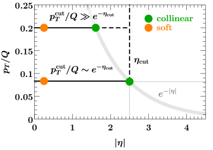
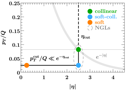
Figure -1138: Illustration of the parametric regimes for a jet veto with a jet rapidity cut. Emissions above the black solid lines are vetoed as pT>pTcutsubscript𝑝𝑇superscriptsubscript𝑝𝑇cutp_{T}>p_{T}^{\rm cut} up to |η|<ηcut=2.5𝜂subscript𝜂cut2.5\lvert\eta\rvert<\eta_{\rm cut}=2.5. The thick gray line corresponds to pT/Q=e|η|subscript𝑝𝑇𝑄superscript𝑒𝜂p_{T}/Q=e^{-\lvert\eta\rvert}, and emissions above and to the right of it are power suppressed. The colored circles indicate the relevant modes in the effective theory for a given hierarchy between pTcut/Qsuperscriptsubscript𝑝𝑇cut𝑄p_{T}^{\rm cut}/Q and eηcutsuperscript𝑒subscript𝜂cute^{-\eta_{\rm cut}}. For pTcut=25GeVsuperscriptsubscript𝑝𝑇cut25GeVp_{T}^{\rm cut}=25\,\mathrm{GeV}, the given examples for pTcut/Qsuperscriptsubscript𝑝𝑇cut𝑄p_{T}^{\rm cut}/Q correspond to Q=125GeV𝑄125GeVQ=125\,\mathrm{GeV} (left panel, upper case), Q=300GeV𝑄300GeVQ=300\,\mathrm{GeV} (left panel, lower case), Q=1TeV𝑄1TeVQ=1\,\mathrm{TeV} (right panel).

We consider exclusive 0-jet cross sections, where the veto is applied by identifying jets with radius R𝑅R (the details of the jet-clustering algorithm are not relevant at the order we are working) and cutting on the transverse momentum pTjetsuperscriptsubscript𝑝𝑇jetp_{T}^{\rm jet} of the leading jet within |ηjet|<ηcutsubscript𝜂jetsubscript𝜂cut\lvert\eta_{\rm jet}\rvert<\eta_{\rm cut},

maxkjets:|ηk|<ηcut|pT,k|<pTcut.subscript:𝑘jetssubscript𝜂𝑘subscript𝜂cutsubscript𝑝𝑇𝑘superscriptsubscript𝑝𝑇cut\max_{k\in\text{jets}:\,\lvert\eta_{k}\rvert<\eta_{\rm cut}}\lvert\vec{p}_{T,k}\rvert<p_{T}^{\rm cut}\,. (2.1)

The resulting constraints on the rapidities and transverse momenta of initial-state radiation (ISR) are displayed as black lines in figure -1138. We can identify two distinct power-counting parameters that govern the typical angular size of energetic collinear ISR with energy EQsimilar-to𝐸𝑄E\sim Q, where Q𝑄Q is the momentum transferred in the hard interaction: First, the pTsubscript𝑝𝑇p_{T} of the emissions is constrained by pT<pTcutsubscript𝑝𝑇superscriptsubscript𝑝𝑇cutp_{T}<p_{T}^{\rm cut} for |η|<ηcut𝜂subscript𝜂cut\lvert\eta\rvert<\eta_{\rm cut}, corresponding to a maximum opening angle

pTEpTcutQ.less-than-or-similar-tosubscript𝑝𝑇𝐸superscriptsubscript𝑝𝑇cut𝑄\frac{p_{T}}{E}\lesssim\frac{p_{T}^{\rm cut}}{Q}\,. (2.2)

Second, the pTsubscript𝑝𝑇p_{T} of an energetic emission at rapidity η𝜂\eta is parametrically pTQe|η|similar-tosubscript𝑝𝑇𝑄superscript𝑒𝜂p_{T}\sim Qe^{-\lvert\eta\rvert}. The rapidity cut removes the first constraint for |η|>ηcut𝜂subscript𝜂cut\lvert\eta\rvert>\eta_{\rm cut}. Hence, if ηcutsubscript𝜂cut\eta_{\rm cut} is central enough, emissions beyond ηcutsubscript𝜂cut\eta_{\rm cut} can reach a characteristic pTQe|ηcut|less-than-or-similar-tosubscript𝑝𝑇𝑄superscript𝑒subscript𝜂cutp_{T}\lesssim Qe^{-\lvert\eta_{\rm cut}\rvert}, corresponding to a maximum opening angle

pTEeηcut.less-than-or-similar-tosubscript𝑝𝑇𝐸superscript𝑒subscript𝜂cut\frac{p_{T}}{E}\lesssim e^{-\eta_{\rm cut}}\,. (2.3)

There are three parametric regimes for pTcut/Qsuperscriptsubscript𝑝𝑇cut𝑄p_{T}^{\rm cut}/Q and eηcutsuperscript𝑒subscript𝜂cute^{-\eta_{\rm cut}}, which are illustrated in figure -1138 for ηcut=2.5subscript𝜂cut2.5\eta_{\rm cut}=2.5. The thick black lines show the veto for different values of pTcut/Qsuperscriptsubscript𝑝𝑇cut𝑄p_{T}^{\rm cut}/Q. The thick gray curve shows the relation pT/Q=e|η|subscript𝑝𝑇𝑄superscript𝑒𝜂p_{T}/Q=e^{-\lvert\eta\rvert}, while the thin gray lines show the values of ηcutsubscript𝜂cut\eta_{\rm cut} and pT/Q=eηcutsubscript𝑝𝑇𝑄superscript𝑒subscript𝜂cutp_{T}/Q=e^{-\eta_{\rm cut}}.

The first parametric regime is pTcut/Qeηcutmuch-greater-thansuperscriptsubscript𝑝𝑇cut𝑄superscript𝑒subscript𝜂cutp_{T}^{\rm cut}/Q\gg e^{-\eta_{\rm cut}}. As we will demonstrate in section 2.2, in this regime effects due to the rapidity cut are power suppressed by Qeηcut/pTcut𝑄superscript𝑒subscript𝜂cutsuperscriptsubscript𝑝𝑇cutQe^{-\eta_{\rm cut}}/p_{T}^{\rm cut}. Hence, they can be treated as a fixed-order power correction to the standard jet-veto resummation, which implicitly works in the limit ηcut=subscript𝜂cut\eta_{\rm cut}=\infty. For Higgs measurements with pTcut=25GeVsuperscriptsubscript𝑝𝑇cut25GeVp_{T}^{\rm cut}=25\,\mathrm{GeV}, ηcut=4.5subscript𝜂cut4.5\eta_{\rm cut}=4.5, QmH=125GeV𝑄subscript𝑚𝐻125GeVQ\equiv m_{H}=125\,\mathrm{GeV}, this parametric assumption is well justified, as mHeηcut/pTcut5%similar-tosubscript𝑚𝐻superscript𝑒subscript𝜂cutsuperscriptsubscript𝑝𝑇cutpercent5m_{H}e^{-\eta_{\rm cut}}/p_{T}^{\rm cut}\sim 5\%.

For heavier final states and/or more central rapidity cuts the relevant parametric regime is pTcut/Qeηcutsimilar-tosuperscriptsubscript𝑝𝑇cut𝑄superscript𝑒subscript𝜂cutp_{T}^{\rm cut}/Q\sim e^{-\eta_{\rm cut}}. This is the case for example for Q=1TeV𝑄1TeVQ=1\,\mathrm{TeV} and ηcut=4.5subscript𝜂cut4.5\eta_{\rm cut}=4.5 or Q=125GeV𝑄125GeVQ=125\,\mathrm{GeV} and ηcut=2.5subscript𝜂cut2.5\eta_{\rm cut}=2.5 at pTcut=25GeVsuperscriptsubscript𝑝𝑇cut25GeVp_{T}^{\rm cut}=25\,\mathrm{GeV}. In section 2.3, we show that in this regime the rapidity cut effects must be treated as a leading-power correction, and that they can be seamlessly incorporated into the existing jet-veto resummation without rapidity cut. We will see that they affect only the boundary terms in the resummed cross section, but not the anomalous dimensions and evolution factors. Hence, they start contributing at NLL or NNLL.

Finally in section 2.4, we discuss the parametric regime pTcut/Qeηcutmuch-less-thansuperscriptsubscript𝑝𝑇cut𝑄superscript𝑒subscript𝜂cutp_{T}^{\rm cut}/Q\ll e^{-\eta_{\rm cut}}. This case is conceptually interesting, since logarithms of the ratio of scales Qeηcut𝑄superscript𝑒subscript𝜂cutQe^{-\eta_{\rm cut}} and pTcutsuperscriptsubscript𝑝𝑇cutp_{T}^{\rm cut} appear, changing the logarithmic structure already at leading-logarithmic (LL) order. In addition, formally large nonglobal logarithms of the same ratio appear. This regime is of very limited phenomenological relevance for typical jet-binned analyses at the LHC. For example, for ηcut=2.3subscript𝜂cut2.3\eta_{\rm cut}=2.3 corresponding to eηcut=0.1superscript𝑒subscript𝜂cut0.1e^{-\eta_{\rm cut}}=0.1, it would require an extremely tight jet veto pTcut0.1Qmuch-less-thansuperscriptsubscript𝑝𝑇cut0.1𝑄p_{T}^{\rm cut}\ll 0.1\,Q, which is unrealistic as it would leave almost no signal in the 00-jet cross section. For the purpose of explicitly probing this regime experimentally, one could lower ηcut1.01.5similar-to-or-equalssubscript𝜂cut1.01.5\eta_{\rm cut}\simeq 1.0-1.5, such that the jet veto only acts on radiation in the very central region.

2.2 Regime 1: 𝒑𝑻𝐜𝐮𝐭/𝑸𝒆𝜼𝐜𝐮𝐭much-greater-thansuperscriptsubscript𝒑𝑻𝐜𝐮𝐭𝑸superscript𝒆subscript𝜼𝐜𝐮𝐭p_{T}^{\rm cut}/Q\gg e^{-\eta_{\rm cut}} (standard jet veto resummation)

As usual, the scaling of the modes in the EFT follows from the nontrivial constraints imposed on emissions by the measurement. Soft emissions at central rapidities are always restricted by the jet veto. Collinear emissions with energy Qsimilar-toabsent𝑄\sim Q and rapidity η𝜂\eta have a transverse momentum Qe|η|similar-toabsent𝑄superscript𝑒𝜂\sim Qe^{-\lvert\eta\rvert} and are constrained by the measurement if Qe|η|pTcutsimilar-to𝑄superscript𝑒𝜂superscriptsubscript𝑝𝑇cutQe^{-\lvert\eta\rvert}\sim p_{T}^{\rm cut}, which determines their scaling. Since QeηcutpTcutmuch-less-than𝑄superscript𝑒subscript𝜂cutsuperscriptsubscript𝑝𝑇cutQe^{-\eta_{\rm cut}}\ll p_{T}^{\rm cut}, these collinear modes are parametrically not forward enough to be sensitive to the rapidity cut, such that the description of their dynamics is simply governed by the power counting in pTcut/Qsuperscriptsubscript𝑝𝑇cut𝑄p_{T}^{\rm cut}/Q. The relevant EFT modes in this regime are thus the same as for a jet veto without any rapidity cut,

soft: pμ(pTcut,pTcut,pTcut),similar-tosuperscript𝑝𝜇superscriptsubscript𝑝𝑇cutsuperscriptsubscript𝑝𝑇cutsuperscriptsubscript𝑝𝑇cut\displaystyle\quad p^{\mu}\sim\Bigl{(}p_{T}^{\rm cut},p_{T}^{\rm cut},p_{T}^{\rm cut}\Bigr{)}\,,
na-collinear:subscript𝑛𝑎-collinear:\displaystyle n_{a}\text{-collinear:} pμ((pTcut)2Q,Q,pTcut),similar-tosuperscript𝑝𝜇superscriptsuperscriptsubscript𝑝𝑇cut2𝑄𝑄superscriptsubscript𝑝𝑇cut\displaystyle\quad p^{\mu}\sim\Bigl{(}\tfrac{(p_{T}^{\rm cut})^{2}}{Q},Q,p_{T}^{\rm cut}\Bigr{)}\,,
nb-collinear:subscript𝑛𝑏-collinear:\displaystyle n_{b}\text{-collinear:} pμ(Q,(pTcut)2Q,pTcut).similar-tosuperscript𝑝𝜇𝑄superscriptsuperscriptsubscript𝑝𝑇cut2𝑄superscriptsubscript𝑝𝑇cut\displaystyle\quad p^{\mu}\sim\Bigl{(}Q,\tfrac{(p_{T}^{\rm cut})^{2}}{Q},p_{T}^{\rm cut}\Bigr{)}\,. (2.4)

Here and below, we give the scaling of momenta in terms of light-cone components defined as (with nna𝑛subscript𝑛𝑎n\equiv n_{a}, n¯nb¯𝑛subscript𝑛𝑏\bar{n}\equiv n_{b}),

pμ=n¯pnμ2+npn¯μ2+pμ(np,n¯p,p)(p+,p,p).superscript𝑝𝜇¯𝑛𝑝superscript𝑛𝜇2𝑛𝑝superscript¯𝑛𝜇2subscriptsuperscript𝑝𝜇perpendicular-to𝑛𝑝¯𝑛𝑝subscript𝑝perpendicular-tosuperscript𝑝superscript𝑝subscript𝑝perpendicular-top^{\mu}=\bar{n}\!\cdot\!p\,\frac{n^{\mu}}{2}+n\!\cdot\!p\,\frac{\bar{n}^{\mu}}{2}+p^{\mu}_{\perp}\equiv(n\!\cdot\!p,\bar{n}\!\cdot\!p,\vec{p}_{\perp})\equiv(p^{+},p^{-},\vec{p}_{\perp})\,. (2.5)

In addition, there are the usual inclusive collinear modes that describe the initial protons at the scale ΛQCDsubscriptΛQCD\Lambda_{\mathrm{QCD}}, and which are not specific to our discussion here.

In principle, we can consider collinear emissions that are forward enough to resolve rapidities |η|ηcutsimilar-to𝜂subscript𝜂cut\lvert\eta\rvert\sim\eta_{\rm cut},

na-collinear (ηcut):subscript𝑛𝑎-collinear (ηcut):\displaystyle n_{a}\text{-collinear ($\eta_{\rm cut}$):} pμ(Qe2ηcut,Q,Qeηcut),similar-tosuperscript𝑝𝜇𝑄superscript𝑒2subscript𝜂cut𝑄𝑄superscript𝑒subscript𝜂cut\displaystyle\quad p^{\mu}\sim\Bigl{(}Qe^{-2\eta_{\rm cut}},Q,Qe^{-\eta_{\rm cut}}\Bigr{)}\,,
nb-collinear (ηcut):subscript𝑛𝑏-collinear (ηcut):\displaystyle n_{b}\text{-collinear ($\eta_{\rm cut}$):} pμ(Q,Qe2ηcut,Qeηcut).similar-tosuperscript𝑝𝜇𝑄𝑄superscript𝑒2subscript𝜂cut𝑄superscript𝑒subscript𝜂cut\displaystyle\quad p^{\mu}\sim\Bigl{(}Q,Qe^{-2\eta_{\rm cut}},Qe^{-\eta_{\rm cut}}\Bigr{)}\,. (2.6)

However, since QeηcutpTcutmuch-less-than𝑄superscript𝑒subscript𝜂cutsuperscriptsubscript𝑝𝑇cutQe^{-\eta_{\rm cut}}\ll p_{T}^{\rm cut}, these emissions have too little transverse momentum to be affected by the jet veto, and are therefore unconstrained and integrated over without requiring additional modes in the EFT. To explicitly see that the ηcutsubscript𝜂cut\eta_{\rm cut} dependence is power suppressed, note that the full jet-veto measurement for the collinear modes contains a θ𝜃\theta function

θ(ηcut|η|)=θ(1e|η|ηcut)=1+𝒪(Qeηcut/pTcut),𝜃subscript𝜂cut𝜂𝜃1superscript𝑒𝜂subscript𝜂cut1𝒪𝑄superscript𝑒subscript𝜂cutsuperscriptsubscript𝑝𝑇cut\theta(\eta_{\rm cut}-\lvert\eta\rvert)=\theta(1-e^{\lvert\eta\rvert-\eta_{\rm cut}})=1+\mathcal{O}(Qe^{-\eta_{\rm cut}}/p_{T}^{\rm cut})\,, (2.7)

which thus only induces power corrections in Qeηcut/pTcut𝑄superscript𝑒subscript𝜂cutsuperscriptsubscript𝑝𝑇cutQe^{-\eta_{\rm cut}}/p_{T}^{\rm cut}.

Therefore, at leading order in the power expansion,111As discussed in refs. [8, 13], one formally needs to count R1much-less-than𝑅1R\ll 1 to avoid soft-collinear mixing terms of 𝒪(R2)𝒪superscript𝑅2\mathcal{O}(R^{2}). A detailed discussion of possible approaches to include them at 𝒪(αs2)𝒪superscriptsubscript𝛼𝑠2\mathcal{O}(\alpha_{s}^{2}) can be found in ref. [28]. we recover the factorization for the 0-jet cross section with ηcut=subscript𝜂cut\eta_{\rm cut}=\infty [8, 7, 13],

σ0(pTcut,ηcut,R,Φ)subscript𝜎0superscriptsubscript𝑝𝑇cutsubscript𝜂cut𝑅Φ\displaystyle\sigma_{0}(p_{T}^{\rm cut},\eta_{\rm cut},R,\Phi) =Hκ(Φ,μ)Ba(pTcut,R,ωa,μ,ν)Bb(pTcut,R,ωb,μ,ν)Sκ(pTcut,R,μ,ν)absentsubscript𝐻𝜅Φ𝜇subscript𝐵𝑎superscriptsubscript𝑝𝑇cut𝑅subscript𝜔𝑎𝜇𝜈subscript𝐵𝑏superscriptsubscript𝑝𝑇cut𝑅subscript𝜔𝑏𝜇𝜈subscript𝑆𝜅superscriptsubscript𝑝𝑇cut𝑅𝜇𝜈\displaystyle=H_{\kappa}(\Phi,\mu)\,B_{a}(p_{T}^{\rm cut},R,\omega_{a},\mu,\nu)\,B_{b}(p_{T}^{\rm cut},R,\omega_{b},\mu,\nu)\,S_{\kappa}(p_{T}^{\rm cut},R,\mu,\nu)
×[1+𝒪(pTcutQ,QeηcutpTcut,R2)].absentdelimited-[]1𝒪superscriptsubscript𝑝𝑇cut𝑄𝑄superscript𝑒subscript𝜂cutsuperscriptsubscript𝑝𝑇cutsuperscript𝑅2\displaystyle\quad\times\biggl{[}1+\mathcal{O}\Bigl{(}\frac{p_{T}^{\rm cut}}{Q},\frac{Qe^{-\eta_{\rm cut}}}{p_{T}^{\rm cut}},R^{2}\Bigr{)}\biggr{]}\,. (2.8)

The hard function Hκsubscript𝐻𝜅H_{\kappa} contains the short-distance matrix element for producing a color-singlet final state and depends on the hard kinematic phase space ΦΦ\Phi, which encodes e.g. the total rapidity Y𝑌Y and invariant mass Q𝑄Q of the color-singlet final state. The soft function Sκsubscript𝑆𝜅S_{\kappa} encodes soft radiation restricted by pTcutsuperscriptsubscript𝑝𝑇cutp_{T}^{\rm cut}. The partonic channel is denoted by κ𝜅\kappa and is implicitly summed over (if necessary). The beam functions Ba,bsubscript𝐵𝑎𝑏B_{a,b} are forward proton matrix elements of collinear SCET fields and encode the perturbative collinear ISR constrained by pTcutsuperscriptsubscript𝑝𝑇cutp_{T}^{\rm cut} as well as the unconstrained ISR below that scale down to the nonperturbative scale of the PDFs [4]. In eq. (2.2), they are evaluated at ωa,b=Qe±Ysubscript𝜔𝑎𝑏𝑄superscript𝑒plus-or-minus𝑌\omega_{a,b}=Qe^{\pm Y}. They are given by a convolution of perturbative matching coefficients ijsubscript𝑖𝑗\mathcal{I}_{ij}, which encode the pTcutsuperscriptsubscript𝑝𝑇cutp_{T}^{\rm cut} constraint, and the standard inclusive quark and gluon PDFs fjsubscript𝑓𝑗f_{j},

Bi(pTcut,R,ω,μ,ν)=jx1dzzij(pTcut,R,ω,z,μ,ν)fj(ωzEcm,μ)[1+𝒪(ΛQCDpTcut)].subscript𝐵𝑖superscriptsubscript𝑝𝑇cut𝑅𝜔𝜇𝜈subscript𝑗subscriptsuperscript1𝑥d𝑧𝑧subscript𝑖𝑗superscriptsubscript𝑝𝑇cut𝑅𝜔𝑧𝜇𝜈subscript𝑓𝑗𝜔𝑧subscript𝐸cm𝜇delimited-[]1𝒪subscriptΛQCDsuperscriptsubscript𝑝𝑇cut\displaystyle B_{i}(p_{T}^{\rm cut},R,\omega,\mu,\nu)=\sum_{j}\int^{1}_{x}\frac{\mathrm{d}z}{z}\,\mathcal{I}_{ij}(p_{T}^{\rm cut},R,\omega,z,\mu,\nu)\,f_{j}\Bigl{(}\frac{\omega}{zE_{\mathrm{cm}}},\mu\Bigr{)}\biggl{[}1+\mathcal{O}\Bigl{(}\frac{\Lambda_{\mathrm{QCD}}}{p_{T}^{\rm cut}}\Bigr{)}\biggr{]}\,. (2.9)

As discussed in detail in ref. [13], all logarithms of the ratio pTcut/Qsuperscriptsubscript𝑝𝑇cut𝑄p_{T}^{\rm cut}/Q in eq. (2.2) are resummed by evaluating each of the hard, beam, and soft functions at their characteristic virtuality and rapidity scales,

μHQ=ωaωb,μBμSpTcut,νBQ,νSpTcut,formulae-sequencesimilar-tosubscript𝜇𝐻𝑄subscript𝜔𝑎subscript𝜔𝑏similar-tosubscript𝜇𝐵subscript𝜇𝑆similar-tosuperscriptsubscript𝑝𝑇cutformulae-sequencesimilar-tosubscript𝜈𝐵𝑄similar-tosubscript𝜈𝑆superscriptsubscript𝑝𝑇cut\displaystyle\mu_{H}\sim Q=\sqrt{\omega_{a}\omega_{b}}\,,\quad\mu_{B}\sim\mu_{S}\sim p_{T}^{\rm cut}\,,\quad\nu_{B}\sim Q\,,\quad\nu_{S}\sim p_{T}^{\rm cut}\,, (2.10)

and evolving them to common scales μ𝜇\mu, ν𝜈\nu using renormalization group (RG) evolution. The power corrections in eq. (2.2) can be included at fixed order in αssubscript𝛼𝑠\alpha_{s} by matching the resummed result to the corresponding fixed-order result in full QCD. The 𝒪(Qeηcut/pTcut)𝒪𝑄superscript𝑒subscript𝜂cutsuperscriptsubscript𝑝𝑇cut\mathcal{O}(Qe^{-\eta_{\rm cut}}/p_{T}^{\rm cut}) corrections stop being suppressed for large Q𝑄Q, small pTcutsuperscriptsubscript𝑝𝑇cutp_{T}^{\rm cut}, or central ηcutsubscript𝜂cut\eta_{\rm cut}. In the next section, we show that they can be incorporated into the beam functions in eq. (2.9).

2.3 Regime 2: 𝒑𝑻𝐜𝐮𝐭/𝑸𝒆𝜼𝐜𝐮𝐭similar-tosuperscriptsubscript𝒑𝑻𝐜𝐮𝐭𝑸superscript𝒆subscript𝜼𝐜𝐮𝐭p_{T}^{\rm cut}/Q\sim e^{-\eta_{\rm cut}} (𝜼𝐜𝐮𝐭subscript𝜼𝐜𝐮𝐭\eta_{\rm cut} dependent beam functions)

In this regime, the scaling of soft and collinear modes is unchanged from the previous case. However, the characteristic rapidity of the collinear modes now coincides parametrically with ηcutsubscript𝜂cut\eta_{\rm cut}, i.e.,

soft: pμ(pTcut,pTcut,pTcut),similar-tosuperscript𝑝𝜇superscriptsubscript𝑝𝑇cutsuperscriptsubscript𝑝𝑇cutsuperscriptsubscript𝑝𝑇cut\displaystyle\quad p^{\mu}\sim\Bigl{(}p_{T}^{\rm cut},p_{T}^{\rm cut},p_{T}^{\rm cut}\Bigr{)}\,,
na-collinear:subscript𝑛𝑎-collinear:\displaystyle n_{a}\text{-collinear:} pμ((pTcut)2Q,Q,pTcut)(Qe2ηcut,Q,Qeηcut),similar-tosuperscript𝑝𝜇superscriptsuperscriptsubscript𝑝𝑇cut2𝑄𝑄superscriptsubscript𝑝𝑇cutsimilar-to𝑄superscript𝑒2subscript𝜂cut𝑄𝑄superscript𝑒subscript𝜂cut\displaystyle\quad p^{\mu}\sim\Bigl{(}\tfrac{(p_{T}^{\rm cut})^{2}}{Q},Q,p_{T}^{\rm cut}\Bigr{)}\sim\Bigl{(}Qe^{-2\eta_{\rm cut}},Q,Qe^{-\eta_{\rm cut}}\Bigr{)}\,,
nb-collinear:subscript𝑛𝑏-collinear:\displaystyle n_{b}\text{-collinear:} pμ(Q,(pTcut)2Q,pTcut)(Q,Qe2ηcut,Qeηcut).similar-tosuperscript𝑝𝜇𝑄superscriptsuperscriptsubscript𝑝𝑇cut2𝑄superscriptsubscript𝑝𝑇cutsimilar-to𝑄𝑄superscript𝑒2subscript𝜂cut𝑄superscript𝑒subscript𝜂cut\displaystyle\quad p^{\mu}\sim\Bigl{(}Q,\tfrac{(p_{T}^{\rm cut})^{2}}{Q},p_{T}^{\rm cut}\Bigr{)}\sim\Bigl{(}Q,Qe^{-2\eta_{\rm cut}},Qe^{-\eta_{\rm cut}}\Bigr{)}\,. (2.11)

Thus, collinear emissions resolve the rapidity cut, and are constrained by the jet veto for |η|<ηcut𝜂subscript𝜂cut|\eta|<\eta_{\rm cut}, while for |η|>ηcut𝜂subscript𝜂cut|\eta|>\eta_{\rm cut} they are unconstrained. As a result, the cross section factorizes at leading power as

σ0(pTcut,ηcut,R,Φ)subscript𝜎0superscriptsubscript𝑝𝑇cutsubscript𝜂cut𝑅Φ\displaystyle\sigma_{0}(p_{T}^{\rm cut},\eta_{\rm cut},R,\Phi) =Hκ(Φ,μ)Ba(pTcut,ηcut,R,ωa,μ,ν)Bb(pTcut,ηcut,R,ωb,μ,ν)absentsubscript𝐻𝜅Φ𝜇subscript𝐵𝑎superscriptsubscript𝑝𝑇cutsubscript𝜂cut𝑅subscript𝜔𝑎𝜇𝜈subscript𝐵𝑏superscriptsubscript𝑝𝑇cutsubscript𝜂cut𝑅subscript𝜔𝑏𝜇𝜈\displaystyle=H_{\kappa}(\Phi,\mu)\,B_{a}(p_{T}^{\rm cut},\eta_{\rm cut},R,\omega_{a},\mu,\nu)\,B_{b}(p_{T}^{\rm cut},\eta_{\rm cut},R,\omega_{b},\mu,\nu)
×Sκ(pTcut,μ,ν)[1+𝒪(pTcutQ,eηcut,R2)].absentsubscript𝑆𝜅superscriptsubscript𝑝𝑇cut𝜇𝜈delimited-[]1𝒪superscriptsubscript𝑝𝑇cut𝑄superscript𝑒subscript𝜂cutsuperscript𝑅2\displaystyle\quad\times S_{\kappa}(p_{T}^{\rm cut},\mu,\nu)\,\biggl{[}1+\mathcal{O}\Bigl{(}\frac{p_{T}^{\rm cut}}{Q},e^{-\eta_{\rm cut}},R^{2}\Bigr{)}\biggr{]}\,. (2.12)

The beam functions now explicitly depend on both pTcutsuperscriptsubscript𝑝𝑇cutp_{T}^{\rm cut} and ηcutsubscript𝜂cut\eta_{\rm cut}, while the hard and soft functions are unchanged (with their characteristic scales still given by eq. (2.10)). The RG consistency of the cross section fixes the anomalous dimensions of the beam function in terms of those for the soft and hard functions. Thus, the ηcutsubscript𝜂cut\eta_{\rm cut} dependence cannot change the renormalization of the beam function, i.e.,

μddμlnBi(pTcut,ηcut,R,ω,x,μ,ν)𝜇dd𝜇subscript𝐵𝑖superscriptsubscript𝑝𝑇cutsubscript𝜂cut𝑅𝜔𝑥𝜇𝜈\displaystyle\mu\frac{\mathrm{d}}{\mathrm{d}\mu}\ln B_{i}(p_{T}^{\rm cut},\eta_{\rm cut},R,\omega,x,\mu,\nu) =γBi(ω,μ,ν),absentsubscriptsuperscript𝛾𝑖𝐵𝜔𝜇𝜈\displaystyle=\gamma^{i}_{B}(\omega,\mu,\nu)\,,
νddνlnBi(pTcut,ηcut,R,ω,x,μ,ν)𝜈dd𝜈subscript𝐵𝑖superscriptsubscript𝑝𝑇cutsubscript𝜂cut𝑅𝜔𝑥𝜇𝜈\displaystyle\nu\frac{\mathrm{d}}{\mathrm{d}\nu}\ln B_{i}(p_{T}^{\rm cut},\eta_{\rm cut},R,\omega,x,\mu,\nu) =γν,Bi(pTcut,R,μ),absentsubscriptsuperscript𝛾𝑖𝜈𝐵superscriptsubscript𝑝𝑇cut𝑅𝜇\displaystyle=\gamma^{i}_{\nu,B}(p_{T}^{\rm cut},R,\mu)\,, (2.13)

where the anomalous dimensions are the same as in the ηcutsubscript𝜂cut\eta_{\rm cut}\to\infty limit [8, 13],

γBi(ω,μ,ν)subscriptsuperscript𝛾𝑖𝐵𝜔𝜇𝜈\displaystyle\gamma^{i}_{B}(\omega,\mu,\nu) =2Γcuspi[αs(μ)]lnνω+γBi[αs(μ)],absent2subscriptsuperscriptΓ𝑖cuspdelimited-[]subscript𝛼𝑠𝜇𝜈𝜔subscriptsuperscript𝛾𝑖𝐵delimited-[]subscript𝛼𝑠𝜇\displaystyle=2\Gamma^{i}_{\rm cusp}[\alpha_{s}(\mu)]\,\ln\frac{\nu}{\omega}+\gamma^{i}_{B}[\alpha_{s}(\mu)]\,,
γν,Bi(pTcut,R,μ)subscriptsuperscript𝛾𝑖𝜈𝐵superscriptsubscript𝑝𝑇cut𝑅𝜇\displaystyle\gamma^{i}_{\nu,B}(p_{T}^{\rm cut},R,\mu) =2ηΓi(pTcut,μ)+γν,Bi[αs(pTcut),R],absent2superscriptsubscript𝜂Γ𝑖superscriptsubscript𝑝𝑇cut𝜇subscriptsuperscript𝛾𝑖𝜈𝐵subscript𝛼𝑠superscriptsubscript𝑝𝑇cut𝑅\displaystyle=2\eta_{\Gamma}^{i}(p_{T}^{\rm cut},\mu)+\gamma^{i}_{\nu,B}[\alpha_{s}(p_{T}^{\rm cut}),R]\,, (2.14)

and ηΓisuperscriptsubscript𝜂Γ𝑖\eta_{\Gamma}^{i} in the resummed rapidity anomalous dimension is given by

ηΓi(μ0,μ)=μ0μdμμΓcuspi[αs(μ)].superscriptsubscript𝜂Γ𝑖subscript𝜇0𝜇superscriptsubscriptsubscript𝜇0𝜇dsuperscript𝜇superscript𝜇subscriptsuperscriptΓ𝑖cuspdelimited-[]subscript𝛼𝑠superscript𝜇\eta_{\Gamma}^{i}(\mu_{0},\mu)=\int_{\mu_{0}}^{\mu}\!\frac{\mathrm{d}\mu^{\prime}}{\mu^{\prime}}\,\Gamma^{i}_{\rm cusp}[\alpha_{s}(\mu^{\prime})]\,. (2.15)

Hence, the ηcutsubscript𝜂cut\eta_{\rm cut} effects do not affect the RG evolution itself, but only change the beam function boundary conditions, and therefore first appear at NLL. The RG evolution between μBpTcutQeηcutsimilar-tosubscript𝜇𝐵superscriptsubscript𝑝𝑇cutsimilar-to𝑄superscript𝑒subscript𝜂cut\mu_{B}\sim p_{T}^{\rm cut}\sim Qe^{-\eta_{\rm cut}} and μHQsimilar-tosubscript𝜇𝐻𝑄\mu_{H}\sim Q now resums all large logarithms of μB/μHpTcut/Qsimilar-tosubscript𝜇𝐵subscript𝜇𝐻superscriptsubscript𝑝𝑇cut𝑄similar-toabsent\mu_{B}/\mu_{H}\sim p_{T}^{\rm cut}/Q\sim eηcutsuperscript𝑒subscript𝜂cute^{-\eta_{\rm cut}}, while the beam function boundary condition now explicitly depends on the ratio Qeηcut/pTcut𝒪(1)similar-to𝑄superscript𝑒subscript𝜂cutsuperscriptsubscript𝑝𝑇cut𝒪1Qe^{-\eta_{\rm cut}}/p_{T}^{\rm cut}\sim\mathcal{O}(1), which in contrast to regime 1 is not power suppressed anymore.

In analogy to eq. (2.9) the beam functions can be factorized into collinear matching coefficients, which now also depend on ηcutsubscript𝜂cut\eta_{\rm cut}, and the PDFs. We write the matching coefficients as the sum of the usual ηcutsubscript𝜂cut\eta_{\rm cut}-independent matching coefficients plus a correction term that encodes the ηcutsubscript𝜂cut\eta_{\rm cut} dependence,

ij(pTcut,ηcut,R,ω,z,μ,ν)subscript𝑖𝑗superscriptsubscript𝑝𝑇cutsubscript𝜂cut𝑅𝜔𝑧𝜇𝜈\displaystyle\mathcal{I}_{ij}(p_{T}^{\rm cut},\eta_{\rm cut},R,\omega,z,\mu,\nu) =ij(pTcut,R,ω,z,μ,ν)+Δij(pTcut,ηcut,R,ω,z,μ,ν).absentsubscript𝑖𝑗superscriptsubscript𝑝𝑇cut𝑅𝜔𝑧𝜇𝜈Δsubscript𝑖𝑗superscriptsubscript𝑝𝑇cutsubscript𝜂cut𝑅𝜔𝑧𝜇𝜈\displaystyle=\mathcal{I}_{ij}(p_{T}^{\rm cut},R,\omega,z,\mu,\nu)+\Delta\mathcal{I}_{ij}(p_{T}^{\rm cut},\eta_{\rm cut},R,\omega,z,\mu,\nu)\,. (2.16)

The ηcutsubscript𝜂cut\eta_{\rm cut}-independent ijsubscript𝑖𝑗\mathcal{I}_{ij} are given in appendix A.2, and in the following we focus on the ΔijΔsubscript𝑖𝑗\Delta\mathcal{I}_{ij}.

Consistency between the cross sections in eqs. (2.2) and (2.3) implies that ΔijΔsubscript𝑖𝑗\Delta\mathcal{I}_{ij} vanishes as ηcutsubscript𝜂cut\eta_{\rm cut}\to\infty. Specifically, defining

ζcutωeηcut/pTcut,subscript𝜁cut𝜔superscript𝑒subscript𝜂cutsuperscriptsubscript𝑝𝑇cut\zeta_{\rm cut}\equiv\omega e^{-\eta_{\rm cut}}/p_{T}^{\rm cut}\,, (2.17)

the ΔijΔsubscript𝑖𝑗\Delta{\mathcal{I}}_{ij} scale like

Δij(pTcut,ηcut,R,ω,z,μ,ν)𝒪(ζcut)forζcut0,formulae-sequencesimilar-toΔsubscript𝑖𝑗superscriptsubscript𝑝𝑇cutsubscript𝜂cut𝑅𝜔𝑧𝜇𝜈𝒪subscript𝜁cutforsubscript𝜁cut0\displaystyle\Delta\mathcal{I}_{ij}\bigl{(}p_{T}^{\rm cut},\eta_{\rm cut},R,\omega,z,\mu,\nu\bigr{)}\sim\mathcal{O}(\zeta_{\rm cut})\qquad\rm{for}\,\,\zeta_{\rm cut}\to 0\,, (2.18)

which is simply the statement from the previous subsection that the ηcutsubscript𝜂cut\eta_{\rm cut} effects are power suppressed in ζcutsubscript𝜁cut\zeta_{\rm cut} for ζcut1much-less-thansubscript𝜁cut1\zeta_{\rm cut}\ll 1.

In fact, ΔijΔsubscript𝑖𝑗\Delta\mathcal{I}_{ij} vanishes altogether for z>ζcut/(1+ζcut)𝑧subscript𝜁cut1subscript𝜁cutz>\zeta_{\rm cut}/(1+\zeta_{\rm cut}), which can be seen from purely kinematic considerations as follows: For the n𝑛n-collinear sector the term ΔijΔsubscript𝑖𝑗\Delta\mathcal{I}_{ij} accounts for the case where at least one jet with pTjetpTcutsubscriptsuperscript𝑝jet𝑇superscriptsubscript𝑝𝑇cutp^{\rm jet}_{T}\geq p_{T}^{\rm cut} and ηjetηcutsubscript𝜂jetsubscript𝜂cut\eta_{\rm jet}\geq\eta_{\rm cut} is reconstructed (and no jet with ηjet<ηcutsubscript𝜂jetsubscript𝜂cut\eta_{\rm jet}<\eta_{\rm cut}). For R1much-less-than𝑅1R\ll 1 all radiation in this jet has ηηcut𝜂subscript𝜂cut\eta\geq\eta_{\rm cut}, as well. Thus, contributions to ΔijΔsubscript𝑖𝑗\Delta\mathcal{I}_{ij} can only appear if

pTcut|pTjet|kjets|pT,k|=kjetspkeηk,superscriptsubscript𝑝𝑇cutsubscriptsuperscript𝑝jet𝑇subscript𝑘jetssubscript𝑝𝑇𝑘subscript𝑘jetssuperscriptsubscript𝑝𝑘superscript𝑒subscript𝜂𝑘\displaystyle p_{T}^{\rm cut}\leq|\vec{p}^{\,\text{jet}}_{T}|\leq\sum_{k\in\text{jets}}|\vec{p}_{T,k}|=\sum_{k\in\text{jets}}p_{k}^{-}e^{-\eta_{k}}\,, (2.19)

where the second equality follows from the jets being massless for R1much-less-than𝑅1R\ll 1. Rewriting this in terms of momentum fractions pk=zkPn=zkω/zsuperscriptsubscript𝑝𝑘subscript𝑧𝑘superscriptsubscript𝑃𝑛subscript𝑧𝑘𝜔𝑧p_{k}^{-}=z_{k}\,P_{n}^{-}=z_{k}\,\omega/z yields, with kzk+z=1subscript𝑘subscript𝑧𝑘𝑧1\sum_{k}z_{k}+z=1 and Pnsuperscriptsubscript𝑃𝑛P_{n}^{-} the momentum of the initial state proton,

pTcutkjetszkzωeηk1zzωeηcut.superscriptsubscript𝑝𝑇cutsubscript𝑘jetssubscript𝑧𝑘𝑧𝜔superscript𝑒subscript𝜂𝑘1𝑧𝑧𝜔superscript𝑒subscript𝜂cut\displaystyle p_{T}^{\rm cut}\leq\sum_{k\in\text{jets}}\frac{z_{k}}{z}\,\omega e^{-\eta_{k}}\leq\frac{1-z}{z}\,\omega e^{-\eta_{\rm cut}}\,. (2.20)

The second inequality follows from all reconstructed n𝑛n-collinear jets having ηk>ηcutsubscript𝜂𝑘subscript𝜂cut\eta_{k}>\eta_{\rm cut}. This implies that eq. (2.18) is trivially satisfied since the domain of integration in z𝑧z scales as xzζcut𝑥𝑧less-than-or-similar-tosubscript𝜁cutx\leq z\lesssim\zeta_{\rm cut}. Hence ΔijΔsubscript𝑖𝑗\Delta\mathcal{I}_{ij} is parametrically important for ζcutz1similar-tosubscript𝜁cut𝑧similar-to1\zeta_{\rm cut}\sim z\sim 1, but vanishes in the threshold limit z1𝑧1z\to 1. This leads to an additional numerical suppression due to the falloff of the PDFs towards larger partonic momentum fractions.

The RGE of ΔijΔsubscript𝑖𝑗\Delta{\mathcal{I}}_{ij} follows from the beam-function RGE eq. (2.3) and the analogue of the matching onto the PDFs in eq. (2.9). It is given by (with the remaining arguments of ΔijΔsubscript𝑖𝑗\Delta{\mathcal{I}}_{ij} understood)

μddμΔij(z,μ,ν)𝜇dd𝜇Δsubscript𝑖𝑗𝑧𝜇𝜈\displaystyle\mu\frac{\mathrm{d}}{\mathrm{d}\mu}\Delta{\mathcal{I}}_{ij}(z,\mu,\nu) =γBi(ω,μ,ν)Δij(z,μ,ν)kΔik(z,μ,ν)z2Pkj[αs(μ),z],absentsubscriptsuperscript𝛾𝑖𝐵𝜔𝜇𝜈Δsubscript𝑖𝑗𝑧𝜇𝜈subscript𝑘subscripttensor-product𝑧Δsubscript𝑖𝑘𝑧𝜇𝜈2subscript𝑃𝑘𝑗subscript𝛼𝑠𝜇𝑧\displaystyle=\gamma^{i}_{B}(\omega,\mu,\nu)\,\Delta{\mathcal{I}}_{ij}(z,\mu,\nu)-\sum_{k}\Delta{\mathcal{I}}_{ik}(z,\mu,\nu)\otimes_{z}2P_{kj}[\alpha_{s}(\mu),z]\,,
νddνΔij(z,μ,ν)𝜈dd𝜈Δsubscript𝑖𝑗𝑧𝜇𝜈\displaystyle\nu\frac{\mathrm{d}}{\mathrm{d}\nu}\Delta{\mathcal{I}}_{ij}(z,\mu,\nu) =γν,Bi(pTcut,R,μ)Δij(z,μ,ν).absentsubscriptsuperscript𝛾𝑖𝜈𝐵superscriptsubscript𝑝𝑇cut𝑅𝜇Δsubscript𝑖𝑗𝑧𝜇𝜈\displaystyle=\gamma^{i}_{\nu,B}(p_{T}^{\rm cut},R,\mu)\,\Delta{\mathcal{I}}_{ij}(z,\mu,\nu)\,. (2.21)

The Mellin convolution zsubscripttensor-product𝑧\otimes_{z} is defined as

g(z)zh(z)=z1dξξg(ξ)h(zξ),subscripttensor-product𝑧𝑔𝑧𝑧superscriptsubscript𝑧1d𝜉𝜉𝑔𝜉𝑧𝜉g(z)\otimes_{z}h(z)=\int_{z}^{1}\!\frac{\mathrm{d}\xi}{\xi}\,g(\xi)\,h\Bigl{(}\frac{z}{\xi}\Bigr{)}\,, (2.22)

and 2Pij(αs,z)2subscript𝑃𝑖𝑗subscript𝛼𝑠𝑧2P_{ij}(\alpha_{s},z) is the standard PDF anomalous dimension with respect to μ𝜇\mu,

μddμfi(x,μ)=jx1dzz 2Pij[αs(μ),z]fj(xz,μ).𝜇dd𝜇subscript𝑓𝑖𝑥𝜇subscript𝑗superscriptsubscript𝑥1d𝑧𝑧2subscript𝑃𝑖𝑗subscript𝛼𝑠𝜇𝑧subscript𝑓𝑗𝑥𝑧𝜇\mu\frac{\mathrm{d}}{\mathrm{d}\mu}f_{i}(x,\mu)=\sum_{j}\int_{x}^{1}\!\frac{\mathrm{d}z}{z}\,2P_{ij}[\alpha_{s}(\mu),z]\,f_{j}\Bigl{(}\frac{x}{z},\mu\Bigr{)}\,. (2.23)

Note that the RGE in eq. (2.3) does not mix ΔijΔsubscript𝑖𝑗\Delta{\mathcal{I}}_{ij} with ijsubscript𝑖𝑗{\mathcal{I}}_{ij} and therefore does not change the ζcutsubscript𝜁cut\zeta_{\rm cut} scaling in eq. (2.18). Solving eq. (2.3) order by order in perturbation theory, we find the following structure through two loops:

Δij(z)Δsubscript𝑖𝑗𝑧\displaystyle\Delta{\mathcal{I}}_{ij}(z) =αs(μ)4πΔij(1)(z)+αs2(μ)(4π)2Δij(2)(z)+𝒪(αs3),absentsubscript𝛼𝑠𝜇4𝜋Δsuperscriptsubscript𝑖𝑗1𝑧superscriptsubscript𝛼𝑠2𝜇superscript4𝜋2Δsuperscriptsubscript𝑖𝑗2𝑧𝒪superscriptsubscript𝛼𝑠3\displaystyle=\frac{\alpha_{s}(\mu)}{4\pi}\,\Delta{\mathcal{I}}_{ij}^{(1)}(z)+\frac{\alpha_{s}^{2}(\mu)}{(4\pi)^{2}}\,\Delta{\mathcal{I}}_{ij}^{(2)}(z)+\mathcal{O}(\alpha_{s}^{3})\,,
Δij(1)(z)Δsuperscriptsubscript𝑖𝑗1𝑧\displaystyle\Delta{\mathcal{I}}_{ij}^{(1)}(z) =ΔIij(1)(ωeηcutpTcut,z),absentΔsuperscriptsubscript𝐼𝑖𝑗1𝜔superscript𝑒subscript𝜂cutsuperscriptsubscript𝑝𝑇cut𝑧\displaystyle=\Delta I_{ij}^{(1)}\Bigl{(}\frac{\omega e^{-\eta_{\rm cut}}}{p_{T}^{\rm cut}},z\Bigr{)}\,,
Δij(2)(z)Δsuperscriptsubscript𝑖𝑗2𝑧\displaystyle\Delta{\mathcal{I}}_{ij}^{(2)}(z) =lnμpTcut[2Γ0ilnνω+2β0+γB 0i]ΔIij(1)(ωeηcutpTcut,z)absent𝜇superscriptsubscript𝑝𝑇cutdelimited-[]2subscriptsuperscriptΓ𝑖0𝜈𝜔2subscript𝛽0subscriptsuperscript𝛾𝑖𝐵 0Δsuperscriptsubscript𝐼𝑖𝑗1𝜔superscript𝑒subscript𝜂cutsuperscriptsubscript𝑝𝑇cut𝑧\displaystyle=\ln\frac{\mu}{p_{T}^{\rm cut}}\Bigl{[}2\Gamma^{i}_{0}\ln\frac{\nu}{\omega}+2\beta_{0}+\gamma^{i}_{B\,0}\Bigr{]}\,\Delta I_{ij}^{(1)}\Bigl{(}\frac{\omega e^{-\eta_{\rm cut}}}{p_{T}^{\rm cut}},z\Bigr{)}
2lnμpTcutkΔIik(1)(ωeηcutpTcut,z)zPkj(0)(z)+ΔIij(2)(ωeηcutpTcut,R,z),2𝜇superscriptsubscript𝑝𝑇cutsubscript𝑘subscripttensor-product𝑧Δsuperscriptsubscript𝐼𝑖𝑘1𝜔superscript𝑒subscript𝜂cutsuperscriptsubscript𝑝𝑇cut𝑧subscriptsuperscript𝑃0𝑘𝑗𝑧Δsuperscriptsubscript𝐼𝑖𝑗2𝜔superscript𝑒subscript𝜂cutsuperscriptsubscript𝑝𝑇cut𝑅𝑧\displaystyle\quad-2\ln\frac{\mu}{p_{T}^{\rm cut}}\sum_{k}\Delta I_{ik}^{(1)}\Bigl{(}\frac{\omega e^{-\eta_{\rm cut}}}{p_{T}^{\rm cut}},z\Bigr{)}\otimes_{z}P^{(0)}_{kj}(z)+\Delta I_{ij}^{(2)}\Bigl{(}\frac{\omega e^{-\eta_{\rm cut}}}{p_{T}^{\rm cut}},R,z\Bigr{)}\,, (2.24)

where ΔIij(n)Δsuperscriptsubscript𝐼𝑖𝑗𝑛\Delta I_{ij}^{(n)} is the boundary condition of the RGE at μ=pTcut𝜇superscriptsubscript𝑝𝑇cut\mu=p_{T}^{\rm cut}, ν=ω𝜈𝜔\nu=\omega, and the required anomalous dimension coefficients are collected in appendix A.1. By dimensional analysis and boost invariance, ΔIij(n)Δsuperscriptsubscript𝐼𝑖𝑗𝑛\Delta I_{ij}^{(n)} can only depend on ζcut=ωeηcut/pTcutsubscript𝜁cut𝜔superscript𝑒subscript𝜂cutsuperscriptsubscript𝑝𝑇cut\zeta_{\rm cut}=\omega e^{-\eta_{\rm cut}}/p_{T}^{\rm cut} in addition to R𝑅R and z𝑧z.

In appendix A.3 we determine the one-loop contribution ΔIij(1)Δsuperscriptsubscript𝐼𝑖𝑗1\Delta I_{ij}^{(1)}, which has the simple form

ΔIij(1)(ζcut,z)=θ(ζcut1+ζcutz) 2Pij(0)(z)lnζcut(1z)z,Δsubscriptsuperscript𝐼1𝑖𝑗subscript𝜁cut𝑧𝜃subscript𝜁cut1subscript𝜁cut𝑧2subscriptsuperscript𝑃0𝑖𝑗𝑧subscript𝜁cut1𝑧𝑧\displaystyle\Delta I^{(1)}_{ij}\bigl{(}\zeta_{\rm cut},z\bigr{)}=\theta\Bigl{(}\frac{\zeta_{\rm cut}}{1+\zeta_{\rm cut}}-z\Bigr{)}\,2P^{(0)}_{ij}(z)\,\ln\frac{\zeta_{\rm cut}(1-z)}{z}\,, (2.25)

with the one-loop splitting functions Pij(0)(z)subscriptsuperscript𝑃0𝑖𝑗𝑧P^{(0)}_{ij}(z) as given in eq. (A.1). The correction vanishes at the kinematic threshold encoded in the overall θ𝜃\theta-function, which also cuts off the singular distributions in Pij(0)(z)subscriptsuperscript𝑃0𝑖𝑗𝑧P^{(0)}_{ij}(z) at z=1𝑧1z=1. The Mellin convolutions of ΔIik(1)zPkj(0)subscripttensor-product𝑧Δsuperscriptsubscript𝐼𝑖𝑘1subscriptsuperscript𝑃0𝑘𝑗\Delta I_{ik}^{(1)}\otimes_{z}P^{(0)}_{kj} appearing in the coefficient of ln(μ/pTcut)𝜇superscriptsubscript𝑝𝑇cut\ln(\mu/p_{T}^{\rm cut}) in Δij(2)(z)Δsuperscriptsubscript𝑖𝑗2𝑧\Delta{\mathcal{I}}_{ij}^{(2)}(z) are given in appendix A.6.

While the computation of the full two-loop contribution ΔIij(2)Δsuperscriptsubscript𝐼𝑖𝑗2\Delta I_{ij}^{(2)} is beyond the scope of this paper, we analytically compute its leading contribution in the small-R𝑅R limit, which contains a clustering logarithm of R𝑅R. We write the full two-loop result as

ΔIij(2)(ζcut,R,z)Δsubscriptsuperscript𝐼2𝑖𝑗subscript𝜁cut𝑅𝑧\displaystyle\Delta I^{(2)}_{ij}(\zeta_{\rm cut},R,z) =lnRΔIij(2,lnR)(ζcut,z)+ΔIij(2,c)(ζcut,z)+𝒪(R2).absent𝑅Δsubscriptsuperscript𝐼2𝑅𝑖𝑗subscript𝜁cut𝑧Δsubscriptsuperscript𝐼2𝑐𝑖𝑗subscript𝜁cut𝑧𝒪superscript𝑅2\displaystyle=\ln R\,\Delta I^{(2,\ln R)}_{ij}(\zeta_{\rm cut},z)+\Delta I^{(2,c)}_{ij}(\zeta_{\rm cut},z)+\mathcal{O}(R^{2})\,. (2.26)

In the limit R1much-less-than𝑅1R\ll 1, we exploit that for the emission of two close-by collinear partons with relative rapidity ΔηRsimilar-toΔ𝜂𝑅\Delta\eta\sim R, the collinear matrix element factorizes into two sequential collinear splittings at the scale μpTcutsimilar-to𝜇superscriptsubscript𝑝𝑇cut\mu\sim p_{T}^{\rm cut} and μpTcutRsimilar-to𝜇superscriptsubscript𝑝𝑇cut𝑅\mu\sim p_{T}^{\rm cut}R, respectively. This allows us to evaluate the coefficient of lnR𝑅\ln R in a generic two-loop beam function as a convolution of a primary on-shell emission and (the anomalous dimension of) the semi-inclusive jet function of ref. [36]. Specifically, for the case of ΔIij(2)Δsubscriptsuperscript𝐼2𝑖𝑗\Delta I^{(2)}_{ij} we find

ΔIij(2,lnR)(ζcut,z)Δsubscriptsuperscript𝐼2𝑅𝑖𝑗subscript𝜁cut𝑧\displaystyle\Delta I^{(2,\ln R)}_{ij}(\zeta_{\rm cut},z) =θ(ζcut1+ζcutz) 2Pij(0)(z)[θ(zζcut2+ζcut)cijR,cut(zζcut(1z))cijR],absent𝜃subscript𝜁cut1subscript𝜁cut𝑧2subscriptsuperscript𝑃0𝑖𝑗𝑧delimited-[]𝜃𝑧subscript𝜁cut2subscript𝜁cutsubscriptsuperscript𝑐𝑅cut𝑖𝑗𝑧subscript𝜁cut1𝑧subscriptsuperscript𝑐𝑅𝑖𝑗\displaystyle=\theta\Bigl{(}\frac{\zeta_{\rm cut}}{1+\zeta_{\rm cut}}-z\Bigr{)}\,2P^{(0)}_{ij}(z)\Bigl{[}\theta\Bigl{(}z-\frac{\zeta_{\rm cut}}{2+\zeta_{\rm cut}}\Bigr{)}c^{R,\rm cut}_{ij}\Bigl{(}\frac{z}{\zeta_{\rm cut}(1-z)}\Bigr{)}-c^{R}_{ij}\Bigr{]}\,, (2.27)

where the coefficient functions cijR,cutsubscriptsuperscript𝑐𝑅cut𝑖𝑗c^{R,\rm cut}_{ij} are given by

cggR,cut(x)=cqqR,cut(x)subscriptsuperscript𝑐𝑅cut𝑔𝑔𝑥subscriptsuperscript𝑐𝑅cut𝑞𝑞𝑥\displaystyle c^{R,\rm cut}_{gg}(x)=c^{R,\rm cut}_{qq}(x) =21/2xdzz1/2zdzJ[Pgg(0)(zJ)+2nfPqg(0)(zJ)],absent2superscriptsubscript12𝑥d𝑧𝑧superscriptsubscript12𝑧differential-dsubscript𝑧𝐽delimited-[]subscriptsuperscript𝑃0𝑔𝑔subscript𝑧𝐽2subscript𝑛𝑓subscriptsuperscript𝑃0𝑞𝑔subscript𝑧𝐽\displaystyle=-2\int_{1/2}^{x}\!\frac{\mathrm{d}z}{z}\,\int_{1/2}^{z}\!\mathrm{d}z_{J}\Bigl{[}P^{(0)}_{gg}(z_{J})+2n_{f}P^{(0)}_{qg}(z_{J})\Bigr{]}\,,
cgqR,cut(x)=cqgR,cut(x)subscriptsuperscript𝑐𝑅cut𝑔𝑞𝑥subscriptsuperscript𝑐𝑅cut𝑞𝑔𝑥\displaystyle c^{R,\rm cut}_{gq}(x)=c^{R,\rm cut}_{qg}(x) =21/2xdzz1/2zdzJ[Pqq(0)(zJ)+Pgq(0)(zJ)],absent2superscriptsubscript12𝑥d𝑧𝑧superscriptsubscript12𝑧differential-dsubscript𝑧𝐽delimited-[]subscriptsuperscript𝑃0𝑞𝑞subscript𝑧𝐽subscriptsuperscript𝑃0𝑔𝑞subscript𝑧𝐽\displaystyle=-2\int_{1/2}^{x}\!\frac{\mathrm{d}z}{z}\,\int_{1/2}^{z}\!\mathrm{d}z_{J}\Bigl{[}P^{(0)}_{qq}(z_{J})+P^{(0)}_{gq}(z_{J})\Bigr{]}\,, (2.28)

depending on whether the primary emission we split is a gluon (first line) or a quark (second line). Their explicit expressions read

cggR,cut(x)=cqqR,cut(x)subscriptsuperscript𝑐𝑅cut𝑔𝑔𝑥subscriptsuperscript𝑐𝑅cut𝑞𝑞𝑥\displaystyle c^{R,\rm cut}_{gg}(x)=c^{R,\rm cut}_{qq}(x) =2CA[58+π233x+92x22x32ln2x4Li2(x)]absent2subscript𝐶𝐴delimited-[]58superscript𝜋233𝑥92superscript𝑥22superscript𝑥32superscript2𝑥4subscriptLi2𝑥\displaystyle=2C_{A}\Bigl{[}\frac{5}{8}+\frac{\pi^{2}}{3}-3x+\frac{9}{2}x^{2}-2x^{3}-2\ln^{2}x-4\,\textrm{Li}_{2}(x)\Bigr{]}
+2β0[2924ln2+3x32x2+23x3lnx],2subscript𝛽0delimited-[]292423𝑥32superscript𝑥223superscript𝑥3𝑥\displaystyle\quad+2\beta_{0}\Bigl{[}-\frac{29}{24}-\ln 2+3x-\frac{3}{2}x^{2}+\frac{2}{3}x^{3}-\ln x\Bigr{]}\,,
cgqR,cut(x)=cqgR,cut(x)subscriptsuperscript𝑐𝑅cut𝑔𝑞𝑥subscriptsuperscript𝑐𝑅cut𝑞𝑔𝑥\displaystyle c^{R,\rm cut}_{gq}(x)=c^{R,\rm cut}_{qg}(x) =2CF[3+π233ln2+6x3lnx2ln2x4Li2(x)].absent2subscript𝐶𝐹delimited-[]3superscript𝜋23326𝑥3𝑥2superscript2𝑥4subscriptLi2𝑥\displaystyle=2C_{F}\Bigl{[}-3+\frac{\pi^{2}}{3}-3\ln 2+6x-3\ln x-2\ln^{2}x-4\,\textrm{Li}_{2}(x)\Bigr{]}\,. (2.29)

The coefficients cijRsubscriptsuperscript𝑐𝑅𝑖𝑗c^{R}_{ij} in eq. (2.27) are the (in principle known) coefficients of lnR𝑅\ln R in the ηcutsubscript𝜂cut\eta_{\rm cut}-independent two-loop beam function [13, 19], which we also verified.222The coefficient of the cgqRsubscriptsuperscript𝑐𝑅𝑔𝑞c^{R}_{gq} contribution in eq. (39) of ref. [13] has a typo, missing an overall factor of 2. We also find that the CAsubscript𝐶𝐴C_{A} term of the coefficient cqqRsubscriptsuperscript𝑐𝑅𝑞𝑞c^{R}_{qq} in eq. (9) of ref. [19] misses a factor of 1/2121/2 compared to ref. [13] and our result. They satisfy

cijR=limx1cijR,cut(x),subscriptsuperscript𝑐𝑅𝑖𝑗subscript𝑥1subscriptsuperscript𝑐𝑅cut𝑖𝑗𝑥c^{R}_{ij}=\lim_{x\to 1}c^{R,\rm cut}_{ij}(x)\,, (2.30)

and are given by

cggRsubscriptsuperscript𝑐𝑅𝑔𝑔\displaystyle c^{R}_{gg} =cqqR=14[(18π23)CA+(2338ln2)β0],absentsubscriptsuperscript𝑐𝑅𝑞𝑞14delimited-[]18superscript𝜋23subscript𝐶𝐴23382subscript𝛽0\displaystyle=c^{R}_{qq}=\frac{1}{4}\Bigl{[}\Bigl{(}1-\frac{8\pi^{2}}{3}\Bigr{)}C_{A}+\Bigl{(}\frac{23}{3}-8\ln 2\Bigr{)}\beta_{0}\Bigr{]}\,,
cqgRsubscriptsuperscript𝑐𝑅𝑞𝑔\displaystyle c^{R}_{qg} =cgqR=2CF(3π233ln2).absentsubscriptsuperscript𝑐𝑅𝑔𝑞2subscript𝐶𝐹3superscript𝜋2332\displaystyle=c^{R}_{gq}=2C_{F}\Bigl{(}3-\frac{\pi^{2}}{3}-3\ln 2\Bigr{)}\,. (2.31)

Our general setup for computing the small-R𝑅R clustering contributions implies that the coefficient of the lnR𝑅\ln R terms of the two-loop rapidity anomalous dimension must be equal to cggR=cqqRsubscriptsuperscript𝑐𝑅𝑔𝑔subscriptsuperscript𝑐𝑅𝑞𝑞c^{R}_{gg}=c^{R}_{qq}, in agreement with the corresponding result given in refs. [8, 13]. In addition, it also applies to the leading ln2Rsuperscript2𝑅\ln^{2}R and lnR𝑅\ln R terms in the beam functions for rapidity dependent jet vetoes in ref. [28], with which we agree as well.

The R𝑅R-independent term ΔIik(2,c)(ζcut,z)Δsubscriptsuperscript𝐼2𝑐𝑖𝑘subscript𝜁cut𝑧\Delta I^{(2,c)}_{ik}(\zeta_{\rm cut},z) and the 𝒪(R2)𝒪superscript𝑅2\mathcal{O}(R^{2}) terms in eq. (2.26) are currently unknown. Their contribution to the cross section can in principle be obtained numerically from the singular limit of the full-theory calculation at 𝒪(αs2)𝒪superscriptsubscript𝛼𝑠2\mathcal{O}(\alpha_{s}^{2}), as was done for the corresponding ηcutsubscript𝜂cut\eta_{\rm cut}-independent pieces in ref. [13].

Numerical validation.
Refer to caption
Refer to caption
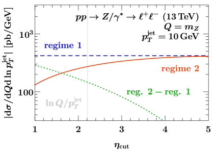
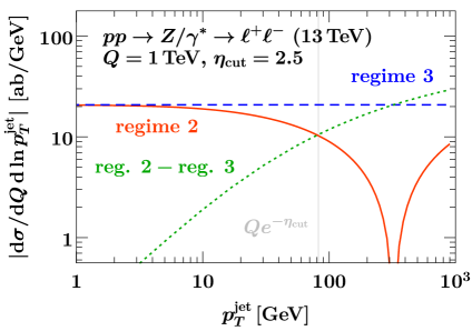
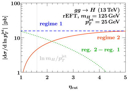
Figure -1137: Comparison of the singular contributions to the fixed 𝒪(αs)𝒪subscript𝛼𝑠\mathcal{O}(\alpha_{s}) (LO1) pTjetsuperscriptsubscript𝑝𝑇jetp_{T}^{\rm jet} spectrum for ggH𝑔𝑔𝐻gg\to H (left) and Drell-Yan (right). The orange solid lines show the singular contributions in regime 2 with ηcutsubscript𝜂cut\eta_{\rm cut} dependent beam functions. The dashed blue lines show the singular contributions in regime 1 in the limit ηcut=subscript𝜂cut\eta_{\rm cut}=\infty, pTcutQeηcutmuch-greater-thansuperscriptsubscript𝑝𝑇cut𝑄superscript𝑒subscript𝜂cutp_{T}^{\rm cut}\gg Qe^{-\eta_{\rm cut}}. Their difference, shown by the dotted green lines, correctly scales as a power in Qeηcut/pTjet𝑄superscript𝑒subscript𝜂cutsuperscriptsubscript𝑝𝑇jetQe^{-\eta_{\rm cut}}/p_{T}^{\rm jet}. The vertical lines indicate the point pTjet=Qeηcutsuperscriptsubscript𝑝𝑇jet𝑄superscript𝑒subscript𝜂cutp_{T}^{\rm jet}=Qe^{-\eta_{\rm cut}}.
Refer to caption
Refer to caption
Refer to caption
Refer to caption
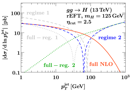
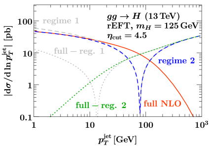
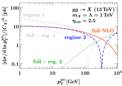
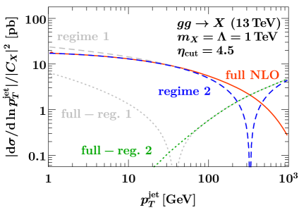
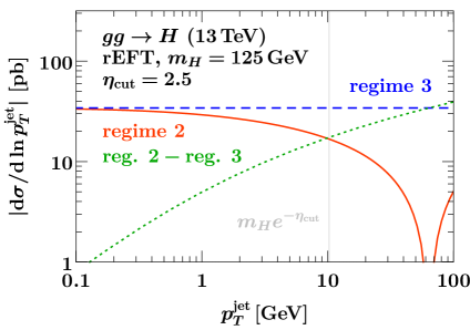
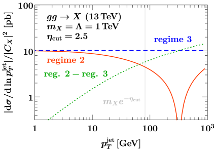
Figure -1136: Comparison of singular and nonsingular contributions to the fixed 𝒪(αs)𝒪subscript𝛼𝑠\mathcal{O}(\alpha_{s}) (LO1) pTjetsuperscriptsubscript𝑝𝑇jetp_{T}^{\rm jet} spectrum with rapidity cut |ηjet|<ηcutsubscript𝜂jetsubscript𝜂cut\lvert\eta_{\rm jet}\rvert<\eta_{\rm cut} for ggH𝑔𝑔𝐻gg\to H (top row) and ggX𝑔𝑔𝑋gg\to X (bottom row), ηcut=2.5subscript𝜂cut2.5\eta_{\rm cut}=2.5 (left) and ηcut=4.5subscript𝜂cut4.5\eta_{\rm cut}=4.5 (right). The orange solid lines show the full results, the dashed blue lines the regime 2 results with ηcutsubscript𝜂cut\eta_{\rm cut} dependent beam functions, and the dotted green lines their difference. The dashed and dotted gray lines show the corresponding regime 1 results, which do not describe the singular behavior of the full cross section for finite ηcutsubscript𝜂cut\eta_{\rm cut}.
Refer to caption
Refer to caption
Refer to caption
Refer to caption
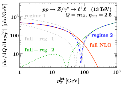
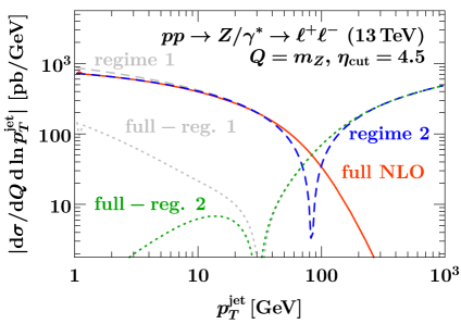
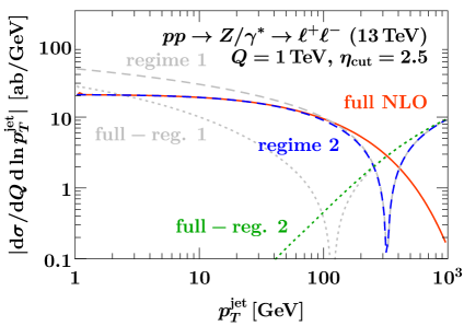
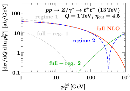
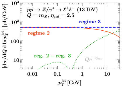
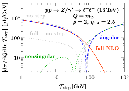
Figure -1135: Comparison of singular and nonsingular contributions to the fixed 𝒪(αs)𝒪subscript𝛼𝑠\mathcal{O}(\alpha_{s}) (LO1) pTjetsuperscriptsubscript𝑝𝑇jetp_{T}^{\rm jet} spectrum with rapidity cut |ηjet|<ηcutsubscript𝜂jetsubscript𝜂cut\lvert\eta_{\rm jet}\rvert<\eta_{\rm cut} for Drell-Yan at Q=mZ𝑄subscript𝑚𝑍Q=m_{Z} (top row) and Q=1TeV𝑄1TeVQ=1\,\mathrm{TeV} (bottom row), ηcut=2.5subscript𝜂cut2.5\eta_{\rm cut}=2.5 (left) and ηcut=4.5subscript𝜂cut4.5\eta_{\rm cut}=4.5 (right). The meaning of the curves are as in figure -1136.

To validate our results numerically and highlight the differences in the singular behavior for regimes 1 and 2, we consider the fixed 𝒪(αs)𝒪subscript𝛼𝑠\mathcal{O}(\alpha_{s}) pTjetsuperscriptsubscript𝑝𝑇jetp_{T}^{\rm jet} spectrum, dσ/dpTjetd𝜎dsuperscriptsubscript𝑝𝑇jet\mathrm{d}\sigma/\mathrm{d}p_{T}^{\rm jet}, where pTjetsuperscriptsubscript𝑝𝑇jetp_{T}^{\rm jet} is the transverse momentum of the leading jet within |ηjet|<ηcutsubscript𝜂jetsubscript𝜂cut\lvert\eta_{\rm jet}\rvert<\eta_{\rm cut}. Its relation to the jet veto cross section with a jet rapidity cut is simply

σ0(pTcut,ηcut,R)=0pTcutdpTjetdσ(ηcut,R)dpTjet.subscript𝜎0superscriptsubscript𝑝𝑇cutsubscript𝜂cut𝑅superscriptsubscript0superscriptsubscript𝑝𝑇cutdifferential-dsuperscriptsubscript𝑝𝑇jetd𝜎subscript𝜂cut𝑅dsuperscriptsubscript𝑝𝑇jet\sigma_{0}(p_{T}^{\rm cut},\eta_{\rm cut},R)=\int_{0}^{p_{T}^{\rm cut}}\!\mathrm{d}p_{T}^{\rm jet}\,\frac{\mathrm{d}\sigma(\eta_{\rm cut},R)}{\mathrm{d}p_{T}^{\rm jet}}\,. (2.32)

At leading power in pTjet/Qsuperscriptsubscript𝑝𝑇jet𝑄p_{T}^{\rm jet}/Q, we obtain it by taking the derivative with respect to pTcutsuperscriptsubscript𝑝𝑇cutp_{T}^{\rm cut} of either eq. (2.3), retaining the exact dependence on ηcutsubscript𝜂cut\eta_{\rm cut} in the beam functions (regime 2), or of eq. (2.2), incurring power corrections in Qeηcut/pTjet𝑄superscript𝑒subscript𝜂cutsuperscriptsubscript𝑝𝑇jetQe^{-\eta_{\rm cut}}/p_{T}^{\rm jet} (regime 1). The numerical results for all singular spectra are obtained with the help of SCETlib [37]. The 𝒪(αs)𝒪subscript𝛼𝑠\mathcal{O}(\alpha_{s}) spectra in full QCD are obtained from MCFM 8.0 [38, 39, 40].

As representative gluon-induced processes, we consider gluon-fusion Higgs production ggH𝑔𝑔𝐻gg\to H at mH=125GeVsubscript𝑚𝐻125GeVm_{H}=125\,\mathrm{GeV} in the infinite top-mass limit, rescaled with the exact LO top-mass dependence for mt=172.5GeVsubscript𝑚𝑡172.5GeVm_{t}=172.5\,\mathrm{GeV} (rEFT). In addition, we consider gluon fusion to a hypothetical heavy color-singlet scalar X𝑋X, ggX𝑔𝑔𝑋gg\to X, mediated by the contact operator

eff=CXΛαsGμνaGa,μνX.subscripteffsubscript𝐶𝑋Λsubscript𝛼𝑠superscriptsubscript𝐺𝜇𝜈𝑎superscript𝐺𝑎𝜇𝜈𝑋\mathcal{L}_{\text{eff}}=-\frac{C_{X}}{\Lambda}\,\alpha_{s}\,G_{\mu\nu}^{a}G^{a,\mu\nu}X\,. (2.33)

We always choose mX=1TeVsubscript𝑚𝑋1TeVm_{X}=1\,\mathrm{TeV}, Λ=1TeVΛ1TeV\Lambda=1\,\mathrm{TeV}, and divide the cross section by |CX|2superscriptsubscript𝐶𝑋2\lvert C_{X}\rvert^{2}. To the order we are working, this is equivalent to setting CX1subscript𝐶𝑋1C_{X}\equiv 1, since CXsubscript𝐶𝑋C_{X} only starts to run at 𝒪(αs2)𝒪superscriptsubscript𝛼𝑠2\mathcal{O}(\alpha_{s}^{2}).333In MCFM 8.0 we mock up this process using a standard-model Higgs with mH=1TeVsubscript𝑚𝐻1TeVm_{H}=1\,\mathrm{TeV} and manually account for the nonzero one-loop contribution from integrating out the top quark in the SM, which differs from our choice of CX=1+𝒪(αs2)subscript𝐶𝑋1𝒪superscriptsubscript𝛼𝑠2C_{X}=1+\mathcal{O}(\alpha_{s}^{2}) for the effective coupling of X𝑋X to gluons. We also checked the results against the native ggX𝑔𝑔𝑋gg\to X support of SusHi 1.6.1 [41, 42, 43, 44]. For quark-induced processes we consider Drell-Yan ppZ/γ+𝑝𝑝𝑍superscript𝛾superscriptsuperscriptpp\to Z/\gamma^{\ast}\to\ell^{+}\ell^{-} at the Z𝑍Z pole (Q=mZ𝑄subscript𝑚𝑍Q=m_{Z}) and at Q=1TeV𝑄1TeVQ=1\,\mathrm{TeV}, where Q=m𝑄subscript𝑚Q=m_{\ell\ell} is the invariant mass of the lepton pair. Here we set all scales to μFO=mHsubscript𝜇FOsubscript𝑚𝐻\mu_{\mathrm{FO}}=m_{H}, mXsubscript𝑚𝑋m_{X}, or Q𝑄Q, respectively. We use PDF4LHC_nnlo_100 [45, 46, 47, 48, 49, 50] NNLO PDFs with αs(mZ)=0.118subscript𝛼𝑠subscript𝑚𝑍0.118\alpha_{s}(m_{Z})=0.118 throughout.

In figure -1137, we compare the regime 2 and regime 1 leading-power (singular) results for dσ/dpTjetd𝜎dsuperscriptsubscript𝑝𝑇jet\mathrm{d}\sigma/\mathrm{d}p_{T}^{\rm jet} at fixed pTjetsuperscriptsubscript𝑝𝑇jetp_{T}^{\rm jet} as a function of ηcutsubscript𝜂cut\eta_{\rm cut} for ggH𝑔𝑔𝐻gg\to H and Drell-Yan. The regime 1 result (dashed blue) does not depend on ηcutsubscript𝜂cut\eta_{\rm cut}, while the regime 2 result (solid orange) decreases as ηcutsubscript𝜂cut\eta_{\rm cut} becomes more central. The difference between the two (dotted green) has the expected behavior, vanishing as Qeηcut/pTjet𝑄superscript𝑒subscript𝜂cutsuperscriptsubscript𝑝𝑇jetQe^{-\eta_{\rm cut}}/p_{T}^{\rm jet} for ηcutsubscript𝜂cut\eta_{\rm cut}\to\infty. We observe that regime 1 is applicable beyond ηcut4greater-than-or-equivalent-tosubscript𝜂cut4\eta_{\rm cut}\gtrsim 4, where the difference to regime 2 is suppressed by an order of magnitude.

Another check is provided by comparing the regime 1 and regime 2 singular results to the full QCD result, which is shown in figures -1136 and -1135 for gluon-fusion and Drell-Yan. For ηcut=2.5subscript𝜂cut2.5\eta_{\rm cut}=2.5 (left panels), it is clear that regime 1 (dashed gray) fails to describe the singular limit of full QCD, with their difference (dotted gray) diverging for pTjet0superscriptsubscript𝑝𝑇jet0p_{T}^{\rm jet}\to 0 like an inverse power of pTjetsuperscriptsubscript𝑝𝑇jetp_{T}^{\rm jet} as expected. While the singular mismatch becomes less pronounced for ηcut=4.5subscript𝜂cut4.5\eta_{\rm cut}=4.5 (right panels), the uncanceled singular contributions are still clearly visible in the difference. On the other hand, regime 2 (dashed blue) correctly reproduces the singular limit pTjet0superscriptsubscript𝑝𝑇jet0p_{T}^{\rm jet}\to 0, with the difference (dotted green) vanishing like a power of pTjetsuperscriptsubscript𝑝𝑇jetp_{T}^{\rm jet} as it must. This provides a strong check of the intricate pTcutsuperscriptsubscript𝑝𝑇cutp_{T}^{\rm cut} dependence encoded in our 𝒪(αs)𝒪subscript𝛼𝑠\mathcal{O}(\alpha_{s}) results for ΔijΔsubscript𝑖𝑗\Delta\mathcal{I}_{ij}. (The power corrections in eηcutsuperscript𝑒subscript𝜂cute^{-\eta_{\rm cut}}, which are present in regime 2, drop out when taking the derivative of the fixed-order cumulant with respect to pTcutsuperscriptsubscript𝑝𝑇cutp_{T}^{\rm cut}.)

Note that at mX=1TeVsubscript𝑚𝑋1TeVm_{X}=1\,\mathrm{TeV} or Q=1TeV𝑄1TeVQ=1\,\mathrm{TeV}, the fixed-order spectrum is completely dominated by the rapidity-cut dependent singular result up to pTjet100GeVless-than-or-similar-tosuperscriptsubscript𝑝𝑇jet100GeVp_{T}^{\rm jet}\lesssim 100\,\mathrm{GeV}. Hence, the resummation should provide a significant improvement over the fixed-order result for typical pTcut50GeVsimilar-tosuperscriptsubscript𝑝𝑇cut50GeVp_{T}^{\rm cut}\sim 50\,\mathrm{GeV}, which we will indeed find in section 4.

2.4 Regime 3: 𝒑𝑻𝐜𝐮𝐭/𝑸𝒆𝜼𝐜𝐮𝐭much-less-thansuperscriptsubscript𝒑𝑻𝐜𝐮𝐭𝑸superscript𝒆subscript𝜼𝐜𝐮𝐭p_{T}^{\rm cut}/Q\ll e^{-\eta_{\rm cut}} (collinear NGLs)

The hierarchy pTcutQeηcutmuch-less-thansuperscriptsubscript𝑝𝑇cut𝑄superscript𝑒subscript𝜂cutp_{T}^{\rm cut}\ll Qe^{-\eta_{\rm cut}} (with eηcut1much-less-thansuperscript𝑒subscript𝜂cut1e^{-\eta_{\rm cut}}\ll 1) exhibits different features than the regimes discussed before. The typical transverse momentum for emissions with |η|>ηcut𝜂subscript𝜂cut|\eta|>\eta_{\rm cut} is parametrically Qe|η|𝑄superscript𝑒𝜂Qe^{-|\eta|}, indicated by the horizontal gray line in figure -1138, which is now much larger than for the strongly constrained emissions at |η|<ηcut𝜂subscript𝜂cut\lvert\eta\rvert<\eta_{\rm cut}. While the soft modes at central rapidities are not affected, there are now two types of collinear modes at forward rapidities with |η|ηcutsimilar-to𝜂subscript𝜂cut\lvert\eta\rvert\sim\eta_{\rm cut},

na-collinear:subscript𝑛𝑎-collinear:\displaystyle n_{a}\text{-collinear:} pμsuperscript𝑝𝜇\displaystyle\quad p^{\mu} Q(e2ηcut,1,eηcut),similar-toabsent𝑄superscript𝑒2subscript𝜂cut1superscript𝑒subscript𝜂cut\displaystyle\sim Q\Bigl{(}e^{-2\eta_{\rm cut}},1,e^{-\eta_{\rm cut}}\Bigr{)}\,,
na-soft-collinear:subscript𝑛𝑎-soft-collinear:\displaystyle n_{a}\text{-soft-collinear:} pμsuperscript𝑝𝜇\displaystyle\quad p^{\mu} (pTcuteηcut,pTcuteηcut,pTcut)=pTcuteηcut(e2ηcut,1,eηcut),similar-toabsentsuperscriptsubscript𝑝𝑇cutsuperscript𝑒subscript𝜂cutsuperscriptsubscript𝑝𝑇cutsuperscript𝑒subscript𝜂cutsuperscriptsubscript𝑝𝑇cutsuperscriptsubscript𝑝𝑇cutsuperscript𝑒subscript𝜂cutsuperscript𝑒2subscript𝜂cut1superscript𝑒subscript𝜂cut\displaystyle\sim\Bigl{(}p_{T}^{\rm cut}e^{-\eta_{\rm cut}},p_{T}^{\rm cut}e^{\eta_{\rm cut}},p_{T}^{\rm cut}\Bigr{)}=p_{T}^{\rm cut}e^{\eta_{\rm cut}}\Bigl{(}e^{-2\eta_{\rm cut}},1,e^{-\eta_{\rm cut}}\Bigr{)}\,, (2.34)

and analogously for the nbsubscript𝑛𝑏n_{b}-collinear sector.

The collinear and soft-collinear modes have the same angular resolution and only differ in their energy. This makes their all-order factorization challenging and leads to the appearance of nonglobal logarithms ln(Qeηcut/pTcut)𝑄superscript𝑒subscript𝜂cutsuperscriptsubscript𝑝𝑇cut\ln(Qe^{-\eta_{\rm cut}}/p_{T}^{\rm cut}) starting at 𝒪(αs2)𝒪superscriptsubscript𝛼𝑠2\mathcal{O}(\alpha_{s}^{2}). Their factorization and resummation requires the marginalization over all possible configurations of energetic collinear emissions, involving soft-collinear matrix elements with a separate Wilson line along each individual energetic collinear emission, see e.g. refs. [51, 52, 53, 54].

Since this regime has no immediate phenomenological relevance, we will not carry out this complete procedure but restrict ourselves to the configuration with soft-collinear Wilson lines along n𝑛n and n¯¯𝑛\bar{n}, i.e, along the two main collinear emitters. This is sufficient for the LL resummation, for isolating the nonglobal effects, and for discussing the relation to the other regimes. Our discussion here is in close analogy to the regime 3 in the factorization of the exclusive jet mass spectrum with small jet radius R𝑅R in ref. [55], where the rapidity cut eηcutsuperscript𝑒subscript𝜂cute^{-\eta_{\rm cut}} here takes the role of R𝑅R there.444The main difference is that here, emissions for |η|<ηcut𝜂subscript𝜂cut|\eta|<\eta_{\rm cut} are constrained by their pTsubscript𝑝𝑇p_{T} relative to the same collinear (beam) direction. In the jet mass case, emissions outside the jet are not constrained by their pTsubscript𝑝𝑇p_{T} relative to the same collinear (jet) direction (but also relative to the beam direction).

The factorized cross section takes the form

σ0(pTcut,ηcut,R,Φ)subscript𝜎0superscriptsubscript𝑝𝑇cutsubscript𝜂cut𝑅Φ\displaystyle\sigma_{0}(p_{T}^{\rm cut},\eta_{\rm cut},R,\Phi) =Hκ(Φ,μ)a(pTcut,ηcut,R,ωa,μ,ν)b(pTcut,ηcut,R,ωb,μ,ν)absentsubscript𝐻𝜅Φ𝜇subscript𝑎superscriptsubscript𝑝𝑇cutsubscript𝜂cut𝑅subscript𝜔𝑎𝜇𝜈subscript𝑏superscriptsubscript𝑝𝑇cutsubscript𝜂cut𝑅subscript𝜔𝑏𝜇𝜈\displaystyle=H_{\kappa}(\Phi,\mu)\,\mathcal{B}_{a}(p_{T}^{\rm cut},\eta_{\rm cut},R,\omega_{a},\mu,\nu)\,\mathcal{B}_{b}(p_{T}^{\rm cut},\eta_{\rm cut},R,\omega_{b},\mu,\nu)
×Sκ(pTcut,R,μ,ν)[1+𝒪(pTcutQeηcut,eηcut,R2)].absentsubscript𝑆𝜅superscriptsubscript𝑝𝑇cut𝑅𝜇𝜈delimited-[]1𝒪superscriptsubscript𝑝𝑇cut𝑄superscript𝑒subscript𝜂cutsuperscript𝑒subscript𝜂cutsuperscript𝑅2\displaystyle\quad\times S_{\kappa}(p_{T}^{\rm cut},R,\mu,\nu)\,\biggl{[}1+\mathcal{O}\Bigl{(}\frac{p_{T}^{\rm cut}}{Qe^{-\eta_{\rm cut}}},e^{-\eta_{\rm cut}},R^{2}\Bigr{)}\biggr{]}\,. (2.35)

The initial-state collinear functions isubscript𝑖\mathcal{B}_{i} encode the contributions of both soft-collinear and energetic collinear modes. They are related to the ηcutsubscript𝜂cut\eta_{\rm cut} dependent beam functions Bisubscript𝐵𝑖B_{i} in eq. (2.3) by an expansion in the limit pTcut/(ωeηcut)1much-less-thansuperscriptsubscript𝑝𝑇cut𝜔superscript𝑒subscript𝜂cut1p_{T}^{\rm cut}/(\omega e^{-\eta_{\rm cut}})\ll 1,

Bi(pTcut,ηcut,R,ω,μ,ν)=i(pTcut,ηcut,R,ω,μ,ν)[1+𝒪(pTcutωeηcut)].subscript𝐵𝑖superscriptsubscript𝑝𝑇cutsubscript𝜂cut𝑅𝜔𝜇𝜈subscript𝑖superscriptsubscript𝑝𝑇cutsubscript𝜂cut𝑅𝜔𝜇𝜈delimited-[]1𝒪superscriptsubscript𝑝𝑇cut𝜔superscript𝑒subscript𝜂cut\displaystyle B_{i}(p_{T}^{\rm cut},\eta_{\rm cut},R,\omega,\mu,\nu)=\mathcal{B}_{i}(p_{T}^{\rm cut},\eta_{\rm cut},R,\omega,\mu,\nu)\biggl{[}1+\mathcal{O}\Bigl{(}\frac{p_{T}^{\rm cut}}{\omega e^{-\eta_{\rm cut}}}\Bigr{)}\biggr{]}\,. (2.36)

Without further factorization, isubscript𝑖\mathcal{B}_{i} contains large unresummed Sudakov double logarithms αsnln2n(pTcut/ωeηcut)superscriptsubscript𝛼𝑠𝑛superscript2𝑛superscriptsubscript𝑝𝑇cut𝜔superscript𝑒subscript𝜂cut\alpha_{s}^{n}\ln^{2n}(p_{T}^{\rm cut}/\omega e^{-\eta_{\rm cut}}). To resum the leading double logarithms, we can decompose isubscript𝑖\mathcal{B}_{i} as

i(pTcut,ηcut,R,ω,μ,ν)subscript𝑖superscriptsubscript𝑝𝑇cutsubscript𝜂cut𝑅𝜔𝜇𝜈\displaystyle\mathcal{B}_{i}(p_{T}^{\rm cut},\eta_{\rm cut},R,\omega,\mu,\nu) =Bi(cut)(ηcut,ω,μ)𝒮i(cut)(pTcut,ηcut,R,μ,ν)absentsubscriptsuperscript𝐵cut𝑖subscript𝜂cut𝜔𝜇subscriptsuperscript𝒮cut𝑖superscriptsubscript𝑝𝑇cutsubscript𝜂cut𝑅𝜇𝜈\displaystyle=B^{(\rm cut)}_{i}(\eta_{\rm cut},\omega,\mu)\,\mathcal{S}^{(\rm cut)}_{i}(p_{T}^{\rm cut},\eta_{\rm cut},R,\mu,\nu)
×[1+i(NG)(pTcutωeηcut,ω,R)].absentdelimited-[]1subscriptsuperscriptNG𝑖superscriptsubscript𝑝𝑇cut𝜔superscript𝑒subscript𝜂cut𝜔𝑅\displaystyle\quad\times\biggl{[}1+\mathcal{B}^{\rm(NG)}_{i}\Bigl{(}\frac{p_{T}^{\rm cut}}{\omega e^{-\eta_{\rm cut}}},\omega,R\Bigr{)}\biggr{]}\,. (2.37)

The function Bi(cut)subscriptsuperscript𝐵cut𝑖B^{(\rm cut)}_{i} mainly describes contributions from the energetic collinear modes. It was dubbed “unmeasured” beam function in refs. [33, 34], in analogy to the unmeasured jet function [56]. At one loop its matching coefficients account for an energetic collinear emission with |η|>ηcut𝜂subscript𝜂cut|\eta|>\eta_{\rm cut}. They are calculated in appendix A.3 and read

gg(cut)(ηcut,ω,z,μ)subscriptsuperscriptcut𝑔𝑔subscript𝜂cut𝜔𝑧𝜇\displaystyle\mathcal{I}^{(\rm cut)}_{gg}(\eta_{\rm cut},\omega,z,\mu) =δ(1z)+αs(μ)CA4π[δ(1z)(4ln2ωeηcutμπ26)\displaystyle=\delta(1-z)+\frac{\alpha_{s}(\mu)\,C_{A}}{4\pi}\biggl{[}\delta(1-z)\biggl{(}4\ln^{2}\frac{\omega e^{-\eta_{\rm cut}}}{\mu}-\frac{\pi^{2}}{6}\biggr{)}
+4Pgg(z)lnωeηcutμz+81(1z)+8(1z2+zz2)ln(1z)]\displaystyle\quad+4P_{gg}(z)\ln\frac{\omega e^{-\eta_{\rm cut}}}{\mu\,z}+8\mathcal{L}_{1}(1-z)+8\Bigl{(}\frac{1}{z}-2+z-z^{2}\Bigr{)}\ln(1-z)\biggr{]}
+𝒪(αs2),𝒪superscriptsubscript𝛼𝑠2\displaystyle\quad+\mathcal{O}(\alpha_{s}^{2})\,,
gq(cut)(ηcut,ω,z,μ)subscriptsuperscriptcut𝑔𝑞subscript𝜂cut𝜔𝑧𝜇\displaystyle\mathcal{I}^{(\rm cut)}_{gq}(\eta_{\rm cut},\omega,z,\mu) =αs(μ)CF4π[4Pgq(z)lnωeηcut(1z)μz+2z]+𝒪(αs2),absentsubscript𝛼𝑠𝜇subscript𝐶𝐹4𝜋delimited-[]4subscript𝑃𝑔𝑞𝑧𝜔superscript𝑒subscript𝜂cut1𝑧𝜇𝑧2𝑧𝒪superscriptsubscript𝛼𝑠2\displaystyle=\frac{\alpha_{s}(\mu)\,C_{F}}{4\pi}\biggl{[}4P_{gq}(z)\ln\frac{\omega e^{-\eta_{\rm cut}}(1-z)}{\mu\,z}+2z\biggr{]}+\mathcal{O}(\alpha_{s}^{2})\,,
qq(cut)(ηcut,ω,z,μ)subscriptsuperscriptcut𝑞𝑞subscript𝜂cut𝜔𝑧𝜇\displaystyle\mathcal{I}^{(\rm cut)}_{qq}(\eta_{\rm cut},\omega,z,\mu) =δ(1z)+αs(μ)CF4π[δ(1z)(4ln2ωeηcutμ6lnωeηcutμπ26)\displaystyle=\delta(1-z)+\frac{\alpha_{s}(\mu)\,C_{F}}{4\pi}\biggl{[}\delta(1-z)\biggl{(}4\ln^{2}\frac{\omega e^{-\eta_{\rm cut}}}{\mu}-6\ln\frac{\omega e^{-\eta_{\rm cut}}}{\mu}-\frac{\pi^{2}}{6}\biggr{)}
+4Pqq(z)lnωeηcutμz+81(1z)4(1+z)ln(1z)+2(1z)]\displaystyle\quad+4P_{qq}(z)\ln\frac{\omega e^{-\eta_{\rm cut}}}{\mu\,z}+8\mathcal{L}_{1}(1-z)-4(1+z)\ln(1-z)+2(1-z)\biggr{]}
+𝒪(αs2),𝒪superscriptsubscript𝛼𝑠2\displaystyle\quad+\mathcal{O}(\alpha_{s}^{2})\,,
qg(cut)(ηcut,ω,z,μ)subscriptsuperscriptcut𝑞𝑔subscript𝜂cut𝜔𝑧𝜇\displaystyle\mathcal{I}^{(\rm cut)}_{qg}(\eta_{\rm cut},\omega,z,\mu) =αs(μ)TF4π[4Pqg(z)lnωeηcut(1z)μz+4z(1z)]+𝒪(αs2),absentsubscript𝛼𝑠𝜇subscript𝑇𝐹4𝜋delimited-[]4subscript𝑃𝑞𝑔𝑧𝜔superscript𝑒subscript𝜂cut1𝑧𝜇𝑧4𝑧1𝑧𝒪superscriptsubscript𝛼𝑠2\displaystyle=\frac{\alpha_{s}(\mu)\,T_{F}}{4\pi}\biggl{[}4P_{qg}(z)\ln\frac{\omega e^{-\eta_{\rm cut}}(1-z)}{\mu\,z}+4z(1-z)\biggr{]}+\mathcal{O}(\alpha_{s}^{2})\,, (2.38)

where n(1z)[lnn(1z)/(1z)]+subscript𝑛1𝑧subscriptdelimited-[]superscript𝑛1𝑧1𝑧\mathcal{L}_{n}(1-z)\equiv[\ln^{n}(1-z)/(1-z)]_{+}, Pij(z)subscript𝑃𝑖𝑗𝑧P_{ij}(z) are the color-stripped LO splitting functions given in eq. (A.1), and the flavor structure is trivial,

q¯iq¯j(cut)=qiqj(cut)=δijqq(cut)+𝒪(αs2),qiq¯j(cut)=q¯iqj(cut)=𝒪(αs2).formulae-sequencesubscriptsuperscriptcutsubscript¯𝑞𝑖subscript¯𝑞𝑗subscriptsuperscriptcutsubscript𝑞𝑖subscript𝑞𝑗subscript𝛿𝑖𝑗subscriptsuperscriptcut𝑞𝑞𝒪superscriptsubscript𝛼𝑠2subscriptsuperscriptcutsubscript𝑞𝑖subscript¯𝑞𝑗subscriptsuperscriptcutsubscript¯𝑞𝑖subscript𝑞𝑗𝒪superscriptsubscript𝛼𝑠2\mathcal{I}^{(\rm cut)}_{\bar{q}_{i}\bar{q}_{j}}=\mathcal{I}^{(\rm cut)}_{q_{i}q_{j}}=\delta_{ij}\mathcal{I}^{(\rm cut)}_{qq}+\mathcal{O}(\alpha_{s}^{2})\,,\qquad\mathcal{I}^{(\rm cut)}_{q_{i}\bar{q}_{j}}=\mathcal{I}^{(\rm cut)}_{\bar{q}_{i}q_{j}}=\mathcal{O}(\alpha_{s}^{2})\,. (2.39)

As argued in ref. [33] the results are directly related to the matching coefficients for fragmenting jet functions in ref. [57].

The function 𝒮i(cut)subscriptsuperscript𝒮cut𝑖\mathcal{S}^{(\rm cut)}_{i} in eq. (2.4) mainly describes contributions from soft-collinear modes. At one loop it accounts for a soft-collinear emission that couples eikonally to the incoming collinear parton i𝑖i. The emission is constrained to pT<pTcutsubscript𝑝𝑇superscriptsubscript𝑝𝑇cutp_{T}<p_{T}^{\rm cut} for |η|<ηcut𝜂subscript𝜂cut|\eta|<\eta_{\rm cut} by the jet veto, and is unconstrained for |η|>ηcut𝜂subscript𝜂cut|\eta|>\eta_{\rm cut}. Using the η𝜂\eta regulator [58, 59] it is given by (see appendix A.4)

𝒮i(cut)(pTcut,ηcut,R,μ,ν)subscriptsuperscript𝒮cut𝑖superscriptsubscript𝑝𝑇cutsubscript𝜂cut𝑅𝜇𝜈\displaystyle\mathcal{S}^{(\rm cut)}_{i}(p_{T}^{\rm cut},\eta_{\rm cut},R,\mu,\nu) =1+αs(μ)4π𝒮i(cut,1)+αs2(μ)(4π)2𝒮(cut,2)+𝒪(αs3),absent1subscript𝛼𝑠𝜇4𝜋subscriptsuperscript𝒮cut1𝑖superscriptsubscript𝛼𝑠2𝜇superscript4𝜋2superscript𝒮cut2𝒪superscriptsubscript𝛼𝑠3\displaystyle=1+\frac{\alpha_{s}(\mu)}{4\pi}\,\mathcal{S}^{(\rm cut,1)}_{i}+\frac{\alpha_{s}^{2}(\mu)}{(4\pi)^{2}}\,\mathcal{S}^{(\rm cut,2)}+\mathcal{O}(\alpha_{s}^{3})\,,
𝒮i(cut,1)(pTcut,ηcut,R,μ,ν)subscriptsuperscript𝒮cut1𝑖superscriptsubscript𝑝𝑇cutsubscript𝜂cut𝑅𝜇𝜈\displaystyle\mathcal{S}^{(\rm cut,1)}_{i}(p_{T}^{\rm cut},\eta_{\rm cut},R,\mu,\nu) =Ci(4ln2pTcutμ8lnpTcutμlnνeηcutμ+π26),absentsubscript𝐶𝑖4superscript2superscriptsubscript𝑝𝑇cut𝜇8superscriptsubscript𝑝𝑇cut𝜇𝜈superscript𝑒subscript𝜂cut𝜇superscript𝜋26\displaystyle=C_{i}\biggl{(}4\ln^{2}\frac{p_{T}^{\rm cut}}{\mu}-8\ln\frac{p_{T}^{\rm cut}}{\mu}\ln\frac{\nu e^{-\eta_{\rm cut}}}{\mu}+\frac{\pi^{2}}{6}\biggr{)}\,, (2.40)

where Ci=CFsubscript𝐶𝑖subscript𝐶𝐹C_{i}=C_{F} for an incoming quark or antiquark and CAsubscript𝐶𝐴C_{A} for an incoming gluon. We checked explicitly that the above results obey the consistency constraint in eq. (2.36). For this purpose, one has to note that eq. (2.25) becomes distribution valued in (1z)1𝑧(1-z) when taking the limit ζcut1much-greater-thansubscript𝜁cut1\zeta_{\rm cut}\gg 1.

At two loops 𝒮i(cut)subscriptsuperscript𝒮cut𝑖\mathcal{S}^{(\rm cut)}_{i} contains a lnR𝑅\ln R enhanced term. Focusing on the constant terms not predicted by the RG evolution, we have

𝒮i(cut,2)(pTcut,ηcut,R,μ=pTcut,ν=μeηcut)=lnR𝒮i(cut,2,lnR)+𝒮i(cut,2,c)+𝒪(R2),\displaystyle\mathcal{S}^{(\rm cut,2)}_{i}(p_{T}^{\rm cut},\eta_{\rm cut},R,\mu=p_{T}^{\rm cut},\nu=\mu e^{\eta_{\rm cut}})=\ln R\,\mathcal{S}^{({\rm cut},2,\ln R)}_{i}+\mathcal{S}^{({\rm cut},2,c)}_{i}+\mathcal{O}(R^{2})\,, (2.41)

with 𝒮i(cut,2,c)subscriptsuperscript𝒮cut2𝑐𝑖\mathcal{S}^{({\rm cut},2,c)}_{i} an unknown two-loop constant. The coefficient of lnR𝑅\ln R is obtained by expanding the lnR𝑅\ln R coefficient in the ηcutsubscript𝜂cut\eta_{\rm cut} dependent beam function [see eqs. (2.27) and (A.21)] to leading power in 1/ζcut1subscript𝜁cut1/\zeta_{\rm cut}. In the limit ζcut1much-greater-thansubscript𝜁cut1\zeta_{\rm cut}\gg 1, the sum Iij(2,lnR)+ΔIij(2,lnR)subscriptsuperscript𝐼2𝑅𝑖𝑗Δsubscriptsuperscript𝐼2𝑅𝑖𝑗I^{(2,\ln R)}_{ij}+\Delta I^{(2,\ln R)}_{ij} becomes proportional to δ(1z)𝛿1𝑧\delta(1-z), as the arguments of both θ𝜃\theta-functions in eq. (2.27) approach z=1𝑧1z=1. The coefficient of δ(1z)𝛿1𝑧\delta(1-z) is then given by the ζcutsubscript𝜁cut\zeta_{\rm cut}\to\infty limit of the integral of ΔIij(2,lnR)Δsubscriptsuperscript𝐼2𝑅𝑖𝑗\Delta I^{(2,\ln R)}_{ij}, which vanishes for ij𝑖𝑗i\neq j and for i=j𝑖𝑗i=j leaves

𝒮i(cut,2,lnR)=8Ci1/21dxxciiR,cut(x)subscriptsuperscript𝒮cut2𝑅𝑖8subscript𝐶𝑖superscriptsubscript121d𝑥𝑥subscriptsuperscript𝑐𝑅cut𝑖𝑖𝑥\displaystyle\mathcal{S}^{({\rm cut},2,\ln R)}_{i}=8C_{i}\int_{1/2}^{1}\!\frac{\mathrm{d}x}{x}c^{R,\rm cut}_{ii}(x) (2.42)
=Ci{CA[1622275489ln2883ln228ζ3]+nfTF[65227+2329ln2+323ln22]}.absentsubscript𝐶𝑖subscript𝐶𝐴delimited-[]16222754892883superscript228subscript𝜁3subscript𝑛𝑓subscript𝑇𝐹delimited-[]6522723292323superscript22\displaystyle=C_{i}\biggl{\{}C_{A}\Bigl{[}\frac{1622}{27}-\frac{548}{9}\ln 2-\frac{88}{3}\ln^{2}2-8\zeta_{3}\Bigr{]}+n_{f}T_{F}\Bigl{[}-\frac{652}{27}+\frac{232}{9}\ln 2+\frac{32}{3}\ln^{2}2\Bigr{]}\biggr{\}}\,.

The anomalous dimensions of Bi(cut)subscriptsuperscript𝐵cut𝑖B^{(\rm cut)}_{i} and 𝒮i(cut)subscriptsuperscript𝒮cut𝑖\mathcal{S}^{(\rm cut)}_{i} have the general structure

γ𝒮cuti(ηcut,μ,ν)subscriptsuperscript𝛾𝑖superscript𝒮cutsubscript𝜂cut𝜇𝜈\displaystyle\gamma^{i}_{\mathcal{S}^{\rm cut}}(\eta_{\rm cut},\mu,\nu) =2Γcuspi[αs(μ)]lnνeηcutμ+γ𝒮cuti[αs(μ)],absent2subscriptsuperscriptΓ𝑖cuspdelimited-[]subscript𝛼𝑠𝜇𝜈superscript𝑒subscript𝜂cut𝜇subscriptsuperscript𝛾𝑖superscript𝒮cutdelimited-[]subscript𝛼𝑠𝜇\displaystyle=2\Gamma^{i}_{\rm cusp}[\alpha_{s}(\mu)]\,\ln\frac{\nu e^{-\eta_{\rm cut}}}{\mu}+\gamma^{i}_{\mathcal{S}^{\rm cut}}[\alpha_{s}(\mu)]\,,
γν,𝒮cuti(pTcut,R,μ)subscriptsuperscript𝛾𝑖𝜈superscript𝒮cutsuperscriptsubscript𝑝𝑇cut𝑅𝜇\displaystyle\gamma^{i}_{\nu,\mathcal{S}^{\rm cut}}(p_{T}^{\rm cut},R,\mu) =2ηΓi(pTcut,μ)+γν,𝒮cuti[αs(pTcut),R],absent2subscriptsuperscript𝜂𝑖Γsuperscriptsubscript𝑝𝑇cut𝜇subscriptsuperscript𝛾𝑖𝜈superscript𝒮cutsubscript𝛼𝑠superscriptsubscript𝑝𝑇cut𝑅\displaystyle=2\eta^{i}_{\Gamma}(p_{T}^{\rm cut},\mu)+\gamma^{i}_{\nu,\mathcal{S}^{\rm cut}}[\alpha_{s}(p_{T}^{\rm cut}),R]\,,
γBcuti(ωeηcut,μ)subscriptsuperscript𝛾𝑖superscript𝐵cut𝜔superscript𝑒subscript𝜂cut𝜇\displaystyle\gamma^{i}_{B^{\rm cut}}\bigl{(}\omega e^{-\eta_{\rm cut}},\mu\bigr{)} =2Γcuspi[αs(μ)]lnμωeηcut+γBcuti[αs(μ)],absent2subscriptsuperscriptΓ𝑖cuspdelimited-[]subscript𝛼𝑠𝜇𝜇𝜔superscript𝑒subscript𝜂cutsubscriptsuperscript𝛾𝑖superscript𝐵cutdelimited-[]subscript𝛼𝑠𝜇\displaystyle=2\Gamma^{i}_{\rm cusp}[\alpha_{s}(\mu)]\,\ln\frac{\mu}{\omega e^{-\eta_{\rm cut}}}+\gamma^{i}_{B^{\rm cut}}[\alpha_{s}(\mu)]\,, (2.43)

where the coefficients of the cusp anomalous dimension follow from our explicit one-loop calculation. Consistency with eq. (2.3) implies

γ𝒮cuti(αs)+γBcuti(αs)subscriptsuperscript𝛾𝑖superscript𝒮cutsubscript𝛼𝑠subscriptsuperscript𝛾𝑖superscript𝐵cutsubscript𝛼𝑠\displaystyle\gamma^{i}_{\mathcal{S}^{\rm cut}}(\alpha_{s})+\gamma^{i}_{B^{\rm cut}}(\alpha_{s}) =γBi(αs),absentsubscriptsuperscript𝛾𝑖𝐵subscript𝛼𝑠\displaystyle=\gamma^{i}_{B}(\alpha_{s})\,,
γν,𝒮cuti(αs,R)subscriptsuperscript𝛾𝑖𝜈superscript𝒮cutsubscript𝛼𝑠𝑅\displaystyle\gamma^{i}_{\nu,\mathcal{S}^{\rm cut}}(\alpha_{s},R) =γν,Bi(αs,R)=12γνi(αs,R).absentsubscriptsuperscript𝛾𝑖𝜈𝐵subscript𝛼𝑠𝑅12subscriptsuperscript𝛾𝑖𝜈subscript𝛼𝑠𝑅\displaystyle=\gamma^{i}_{\nu,B}(\alpha_{s},R)=-\frac{1}{2}\gamma^{i}_{\nu}(\alpha_{s},R)\,. (2.44)

All of the above noncusp anomalous dimensions vanish at one loop. The canonical scales for Bi(cut)subscriptsuperscript𝐵cut𝑖B^{(\rm cut)}_{i} and 𝒮i(cut)subscriptsuperscript𝒮cut𝑖\mathcal{S}^{(\rm cut)}_{i} are

μB(cut)Qeηcut,μ𝒮(cut)pTcut,ν𝒮(cut)pTcuteηcut.formulae-sequencesimilar-tosubscriptsuperscript𝜇cut𝐵𝑄superscript𝑒subscript𝜂cutformulae-sequencesimilar-tosubscriptsuperscript𝜇cut𝒮superscriptsubscript𝑝𝑇cutsimilar-tosubscriptsuperscript𝜈cut𝒮superscriptsubscript𝑝𝑇cutsuperscript𝑒subscript𝜂cut\displaystyle\mu^{(\rm cut)}_{B}\sim Qe^{-\eta_{\rm cut}}\,,\quad\mu^{(\rm cut)}_{\mathcal{S}}\sim p_{T}^{\rm cut}\,,\quad\nu^{(\rm cut)}_{\mathcal{S}}\sim p_{T}^{\rm cut}e^{\eta_{\rm cut}}\,. (2.45)

With these choices and the anomalous dimensions in eq. (2.4) one may resum logarithms of eηcutsuperscript𝑒subscript𝜂cute^{\eta_{\rm cut}}, pTcut/Qsuperscriptsubscript𝑝𝑇cut𝑄p_{T}^{\rm cut}/Q to any logarithmic order, and at LL also logarithms of pTcut/Qeηcutsuperscriptsubscript𝑝𝑇cut𝑄superscript𝑒subscript𝜂cutp_{T}^{\rm cut}/Qe^{-\eta_{\rm cut}}.

Starting at 𝒪(αs2)𝒪superscriptsubscript𝛼𝑠2\mathcal{O}(\alpha_{s}^{2}), the i(NG)subscriptsuperscriptNG𝑖\mathcal{B}^{\rm(NG)}_{i} term in eq. (2.4) contains nonglobal logarithms of the form αsnlnn(pTcut/Qeηcut)superscriptsubscript𝛼𝑠𝑛superscript𝑛superscriptsubscript𝑝𝑇cut𝑄superscript𝑒subscript𝜂cut\alpha_{s}^{n}\ln^{n}(p_{T}^{\rm cut}/Qe^{-\eta_{\rm cut}}). A boost by ηcutsubscript𝜂cut\eta_{\rm cut} translates the measurement into two hemispheres with one loose (η>ηcut𝜂subscript𝜂cut\eta>\eta_{\rm cut}) and one tight constraint (η<ηcut𝜂subscript𝜂cut\eta<\eta_{\rm cut}) on emissions. The nonglobal structure in such a scenario is well understood [60]. Depending on the desired accuracy, the NGLs may be included at fixed order via i(NG)subscriptsuperscriptNG𝑖\mathcal{B}^{\rm(NG)}_{i} as indicated in eq. (2.4), or (partially) summed using more steps in a dressed parton expansion [53].

Note that beyond one loop there is some freedom in the choice of measurement that defines the Bi(cut)subscriptsuperscript𝐵cut𝑖B^{(\rm cut)}_{i} and 𝒮i(cut)subscriptsuperscript𝒮cut𝑖\mathcal{S}^{(\rm cut)}_{i}. In particular, different measurements that reduce to eqs. (2.4) and (2.4) for a single emission could give rise to different results for the two-loop noncusp anomalous dimensions and finite terms because the difference can be absorbed into i(NG)subscriptsuperscriptNG𝑖\mathcal{B}^{\rm(NG)}_{i}. We stress that the result eq. (2.42) for the lnR𝑅\ln R coefficient in the two-loop soft-collinear function is, however, still unique. This is because a lnR𝑅\ln R contribution to (NG)superscriptNG\mathcal{B}^{(\rm NG)} requires a collinear parton in the unconstrained region to emit a soft-collinear gluon into the constrained region, which then undergoes a further collinear splitting. This is only possible starting at 𝒪(αs3)𝒪superscriptsubscript𝛼𝑠3\mathcal{O}(\alpha_{s}^{3}).

Numerical validation.

Refer to caption
Refer to caption
Refer to caption
Refer to caption
Figure -1134: Comparison of the singular contributions to the fixed 𝒪(αs)𝒪subscript𝛼𝑠\mathcal{O}(\alpha_{s}) pTjetsuperscriptsubscript𝑝𝑇jetp_{T}^{\rm jet} spectrum for ggH𝑔𝑔𝐻gg\to H (top left), ggX𝑔𝑔𝑋gg\to X (top right), and Drell-Yan at Q=mZ𝑄subscript𝑚𝑍Q=m_{Z} (bottom left) and Q=1TeV𝑄1TeVQ=1\,\mathrm{TeV} (bottom right). The solid orange lines show the full regime 2 singular spectrum, the blue dashed lines the further factorized regime 3 result. Their difference shown by the dotted green lines vanishes as a power in pTjet/Qeηcutsuperscriptsubscript𝑝𝑇jet𝑄superscript𝑒subscript𝜂cutp_{T}^{\rm jet}/Qe^{-\eta_{\rm cut}} for small pTjetsuperscriptsubscript𝑝𝑇jetp_{T}^{\rm jet}. The vertical lines indicate where the relation pTjet=Qeηcutsuperscriptsubscript𝑝𝑇jet𝑄superscript𝑒subscript𝜂cutp_{T}^{\rm jet}=Qe^{-\eta_{\rm cut}} is satisfied.

To illustrate the numerical relevance of regime 3, we again consider the fixed 𝒪(αs)𝒪subscript𝛼𝑠\mathcal{O}(\alpha_{s}) pTjetsuperscriptsubscript𝑝𝑇jetp_{T}^{\rm jet} spectrum. In regime 2, it is given to leading power in pTjet/Qsuperscriptsubscript𝑝𝑇jet𝑄p_{T}^{\rm jet}/Q by the derivative of eq. (2.3), while in regime 3, it is given to leading power in pTjet/(Qeηcut)superscriptsubscript𝑝𝑇jet𝑄superscript𝑒subscript𝜂cutp_{T}^{\rm jet}/(Qe^{-\eta_{\rm cut}}) by the derivative of eq. (2.4).

In figure -1134 we compare the two results for ηcut=2.5subscript𝜂cut2.5\eta_{\rm cut}=2.5. In regime 3, the 0-jet cross section at 𝒪(αs)𝒪subscript𝛼𝑠\mathcal{O}(\alpha_{s}) contains only single logarithms of pTcutsuperscriptsubscript𝑝𝑇cutp_{T}^{\rm cut}, because the double logarithms cancel between the soft and soft-collinear functions. For this reason, the dashed-blue regime 3 spectrum with respect to lnpTjetsuperscriptsubscript𝑝𝑇jet\ln p_{T}^{\rm jet} is just a constant. The exact regime 2 result (solid orange) becomes well approximated by the further factorized regime 3 expression for pTjet0superscriptsubscript𝑝𝑇jet0p_{T}^{\rm jet}\to 0, with their difference (dotted green) behaving like a power in pTjetsuperscriptsubscript𝑝𝑇jetp_{T}^{\rm jet}. This provides a strong check of the regime 3 ingredients, more precisely, of the pTcutsuperscriptsubscript𝑝𝑇cutp_{T}^{\rm cut} dependence encoded in the soft-collinear function. (Since the beam function in regime 3 is independent of pTcutsuperscriptsubscript𝑝𝑇cutp_{T}^{\rm cut}, it drops out when computing the fixed-order spectrum.)

We also observe that for ggH𝑔𝑔𝐻gg\to H and Drell-Yan at Q=mZ𝑄subscript𝑚𝑍Q=m_{Z}, the regime 3 limit is applicable only at very small pTjet1GeVless-than-or-similar-tosuperscriptsubscript𝑝𝑇jet1GeVp_{T}^{\rm jet}\lesssim 1\,\mathrm{GeV} and already at pTjet1020GeVsimilar-tosuperscriptsubscript𝑝𝑇jet1020GeVp_{T}^{\rm jet}\sim 10-20\,\mathrm{GeV} the power corrections with respect to regime 2 are of the same size as the full regime 2 result. This means that one would have to turn off the additional regime 3 resummation above this region. For ggX𝑔𝑔𝑋gg\to X with mX=1TeVsubscript𝑚𝑋1TeVm_{X}=1\,\mathrm{TeV} and Drell-Yan at Q=1TeV𝑄1TeVQ=1\,\mathrm{TeV}, the canonical regime 3 resummation region, i.e., the region where the regime 3 singular corrections clearly dominate, extends up to pTjet10GeVless-than-or-similar-tosuperscriptsubscript𝑝𝑇jet10GeVp_{T}^{\rm jet}\lesssim 10\,\mathrm{GeV}, while regime 2 power corrections become 𝒪(1)𝒪1\mathcal{O}(1) around pTjet60GeVsimilar-tosuperscriptsubscript𝑝𝑇jet60GeVp_{T}^{\rm jet}\sim 60\,\mathrm{GeV}.

Hence, we find that the additional resummation of logarithms of pTjet/(Qeηcut)superscriptsubscript𝑝𝑇jet𝑄superscript𝑒subscript𝜂cutp_{T}^{\rm jet}/(Qe^{-\eta_{\rm cut}}) in regime 3 is not relevant for jet veto analyses at the LHC, where the lowest jet cuts are pTcut25GeVsimilar-tosuperscriptsubscript𝑝𝑇cut25GeVp_{T}^{\rm cut}\sim 25\,\mathrm{GeV}, for ηcut=2.5subscript𝜂cut2.5\eta_{\rm cut}=2.5 and final states in the Q100GeVsimilar-to𝑄100GeVQ\sim 100\,\mathrm{GeV} range. This also holds for final states at very high invariant mass, e.g. in new physics searches, since in this case one would typically also apply higher jet thresholds to retain enough signal in the 00-jet bin. Realistically, one would not go below pTcut0.1Qsimilar-tosuperscriptsubscript𝑝𝑇cut0.1𝑄p_{T}^{\rm cut}\sim 0.1Q, which means one never enters the limit where the regime 3 resummation is necessary. This of course does not exclude the possibility that measurements designed to probe simultaneously very high Q𝑄Q and very low pTjetsuperscriptsubscript𝑝𝑇jetp_{T}^{\rm jet} could benefit from the regime 3 resummation. To explicitly explore this regime experimentally, the best option is to restrict the jet veto to the very central region with ηcut11.5similar-tosubscript𝜂cut11.5\eta_{\rm cut}\sim 1-1.5.

2.5 Comparison to the literature

Jet vetoes in a restricted rapidity range were already encountered in ref. [33] for the case of dijet production. Without spelling it out explicitly, ref. [33] used a factorization for the regime 3 hierarchy pTcutQeηcutQmuch-less-thansuperscriptsubscript𝑝𝑇cut𝑄superscript𝑒subscript𝜂cutmuch-less-than𝑄p_{T}^{\rm cut}\ll Qe^{-\eta_{\rm cut}}\ll Q, but did not distinguish between the soft and soft-collinear modes necessary in this regime. As a result, parametrically large rapidity logarithms lneηcutsuperscript𝑒subscript𝜂cut\ln e^{\eta_{\rm cut}} were not captured, which are relevant starting at NLL. The numerical results in ref. [33] were obtained for Q1TeVsimilar-to𝑄1TeVQ\sim 1\,\mathrm{TeV}, ηcut=5subscript𝜂cut5\eta_{\rm cut}=5, and pTcut=20superscriptsubscript𝑝𝑇cut20p_{T}^{\rm cut}=20 GeV, which rather corresponds to the opposite regime 1, pTcutQeηcutmuch-greater-thansuperscriptsubscript𝑝𝑇cut𝑄superscript𝑒subscript𝜂cutp_{T}^{\rm cut}\gg Qe^{-\eta_{\rm cut}}. The difference between regimes 1 and 3 already matters at LL.

In ref. [34], the soft and soft-collinear modes in regime 3 are distinguished and the presence of nonglobal logarithms in this regime is recognized. Their factorization for dijet production is carried out at a level analogous to ours in the previous subsection. That is, at NLL and beyond it only captures logarithms of “global” origin, but does not capture nonglobal logarithms that are parametrically of the same size. Our results for the one-loop quark matching coefficients in eq. (2.4) and the one-loop soft-collinear function in eq. (2.4) agree with ref. [34] [see their eqs. (3.27), (B.3), and (B.5)]. Our results for the gluon channels and the two-loop clustering corrections are new.

Ref. [34] does not consider regime 2 as a separate parametric regime. Instead, it attempts to extend the validity of the regime 3 factorization into regime 2. This is done by effectively adding the regime 2 nonsingular corrections appearing in eq. (2.36) to the unmeasured beam functions. Since some of the regime 3 modes become redundant in regime 2, this also requires them to account for a nontrivial soft-collinear zero bin. At fixed order, the sum of all their contributions must reproduce our result for the regime 2 beam function; in appendix A.5 we check that this is indeed the case for the quark matrix elements given in ref. [34]. As we have seen in figure -1134, outside the canonical regime 3, there are large cancellations between the terms that are singular in the regime 3 limit and the remaining regime 2 nonsingular contributions. This means that the distinction between these contributions becomes arbitrary in regime 2 and that they must not be treated differently, as otherwise one risks inducing large miscancellations. (This is completely analogous to the situation when matching to full QCD, in which case the pTcutsuperscriptsubscript𝑝𝑇cutp_{T}^{\rm cut} resummation must be turned off when entering the fixed-order region at large pTcutsuperscriptsubscript𝑝𝑇cutp_{T}^{\rm cut} to properly recover the full-QCD result.) In particular, in regime 2 all contributions that belong to the full ηcutsubscript𝜂cut\eta_{\rm cut}-dependent regime 2 beam function must be evaluated at a common scale μpTcutsimilar-to-or-equals𝜇superscriptsubscript𝑝𝑇cut\mu\simeq p_{T}^{\rm cut} and evolved together according to eq. (2.3). This is not the case in ref. [34], where individual contributions to the regime 2 beam function are evaluated at different scales throughout (μBcutsuperscriptsubscript𝜇𝐵cut\mu_{B}^{\mathrm{cut}} and μ𝒮cutsuperscriptsubscript𝜇𝒮cut\mu_{\mathcal{S}}^{\mathrm{cut}} in our notation).

Recently, the setup of ref. [34] was applied in ref. [35] to the case of transverse energy ETsubscript𝐸𝑇E_{T} in a restricted rapidity range in Drell-Yan. In ref. [35], profile scales are used to combine regimes 3 and 1, requiring that asymptotically μB(cut)=μ𝒮(cut)subscriptsuperscript𝜇cut𝐵subscriptsuperscript𝜇cut𝒮\mu^{(\rm cut)}_{B}=\mu^{(\rm cut)}_{\mathcal{S}} in the regime 1 limit ETQeηcutmuch-greater-thansubscript𝐸𝑇𝑄superscript𝑒subscript𝜂cutE_{T}\gg Qe^{-\eta_{\rm cut}}. While this can alleviate the issue raised above, formally this relation must be satisfied already in regime 2 for ETQeηcutsimilar-tosubscript𝐸𝑇𝑄superscript𝑒subscript𝜂cutE_{T}\sim Qe^{-\eta_{\rm cut}}.

As we have seen in section 2.3, there is no need to distinguish collinear and soft-collinear modes in regime 2. Since for jet-veto analyses regimes 1 and 2 are the phenomenologically relevant ones, doing so unnecessarily complicates the description. Recovering the NNLL structure in regime 2 [see eq. (2.3)] based on regime 3 would be quite challenging due to the intricate nonglobal structure in regime 3. Our dedicated treatment of regime 2 makes the absence of nonglobal logarithms manifest, avoiding the associated complications, and automatically ensures the correct treatment of the regime 2 nonsingular terms. Furthermore, it shows how regime 2 generalizes the well-understood regime 1, and as we will see in the next section allows for the generalization to a step in the jet veto.

Concerning regime 1, ref. [35] also gave an argument that regime 1 holds up to power corrections in Qeηcut/ET𝑄superscript𝑒subscript𝜂cutsubscript𝐸𝑇Qe^{-\eta_{\rm cut}}/E_{T}, which was more intricate due to immediately comparing regime 1 to regime 3. The power suppression of ηcutsubscript𝜂cut\eta_{\rm cut} effects at sufficiently large ηcutsubscript𝜂cut\eta_{\rm cut} was also pointed out briefly in a somewhat different context in ref. [61].

3 Generalization to a step in the jet veto at 𝜼𝐜𝐮𝐭subscript𝜼𝐜𝐮𝐭\eta_{\rm cut}

3.1 Overview of parametric regimes

We now generalize our results to the experimentally relevant scenario of the step-like jet veto illustrated in the right panel of figure -1139. Here, jets with pTjet>pTcutsuperscriptsubscript𝑝𝑇jetsuperscriptsubscript𝑝𝑇cutp_{T}^{\rm jet}>p_{T}^{\rm cut} are vetoed if |ηjet|<ηcutsubscript𝜂jetsubscript𝜂cut|\eta_{\rm jet}|<\eta_{\rm cut}, while for |ηjet|>ηcutsubscript𝜂jetsubscript𝜂cut|\eta_{\rm jet}|>\eta_{\rm cut} the veto is loosened to pTjet>p~Tcut>pTcutsuperscriptsubscript𝑝𝑇jetsuperscriptsubscript~𝑝𝑇cutsuperscriptsubscript𝑝𝑇cutp_{T}^{\rm jet}>\tilde{p}_{T}^{\rm cut}>p_{T}^{\rm cut}. The 0-jet cross section is thus defined by the following measurement:

maxkjets:|ηk|<ηcut|pT,k|<pTcutandmaxkjets:|ηk|>ηcut|pT,k|<p~Tcut.formulae-sequencesubscript:𝑘jetssubscript𝜂𝑘subscript𝜂cutsubscript𝑝𝑇𝑘superscriptsubscript𝑝𝑇cutandsubscript:𝑘jetssubscript𝜂𝑘subscript𝜂cutsubscript𝑝𝑇𝑘superscriptsubscript~𝑝𝑇cut\max_{k\in\text{jets}:\,\lvert\eta_{k}\rvert<\eta_{\rm cut}}\lvert\vec{p}_{T,k}\rvert<p_{T}^{\rm cut}\qquad\text{and}\qquad\max_{k\in\text{jets}:\,\lvert\eta_{k}\rvert>\eta_{\rm cut}}\lvert\vec{p}_{T,k}\rvert<\tilde{p}_{T}^{\rm cut}\,. (3.1)

There are now three relevant power-counting parameters pTcut/Qsuperscriptsubscript𝑝𝑇cut𝑄p_{T}^{\rm cut}/Q, p~Tcut/Qsuperscriptsubscript~𝑝𝑇cut𝑄\tilde{p}_{T}^{\rm cut}/Q, and eηcutsuperscript𝑒subscript𝜂cute^{-\eta_{\rm cut}} with four distinct parametric regimes (assuming pTcutp~Tcutsuperscriptsubscript𝑝𝑇cutsuperscriptsubscript~𝑝𝑇cutp_{T}^{\rm cut}\leq\tilde{p}_{T}^{\rm cut}), illustrated in figure -1133:

  • pTcut/Qp~Tcut/Qeηcutsimilar-tosuperscriptsubscript𝑝𝑇cut𝑄superscriptsubscript~𝑝𝑇cut𝑄similar-tosuperscript𝑒subscript𝜂cutp_{T}^{\rm cut}/Q\sim\tilde{p}_{T}^{\rm cut}/Q\sim e^{-\eta_{\rm cut}} (collinear step, top left),

  • pTcut/Qp~Tcut/Qeηcutmuch-less-thansuperscriptsubscript𝑝𝑇cut𝑄superscriptsubscript~𝑝𝑇cut𝑄similar-tosuperscript𝑒subscript𝜂cutp_{T}^{\rm cut}/Q\ll\tilde{p}_{T}^{\rm cut}/Q\sim e^{-\eta_{\rm cut}} (collinear NGLs, top right),

  • pTcut/Qp~Tcut/Qeηcutsimilar-tosuperscriptsubscript𝑝𝑇cut𝑄superscriptsubscript~𝑝𝑇cut𝑄much-less-thansuperscript𝑒subscript𝜂cutp_{T}^{\rm cut}/Q\sim\tilde{p}_{T}^{\rm cut}/Q\ll e^{-\eta_{\rm cut}} (soft-collinear step, bottom left),

  • pTcut/Qp~Tcut/Qeηcutmuch-less-thansuperscriptsubscript𝑝𝑇cut𝑄superscriptsubscript~𝑝𝑇cut𝑄much-less-thansuperscript𝑒subscript𝜂cutp_{T}^{\rm cut}/Q\ll\tilde{p}_{T}^{\rm cut}/Q\ll e^{-\eta_{\rm cut}} (soft-collinear NGLs, bottom right).

We discuss each of them in turn in the following subsections. For pTcut/Qeηcutsimilar-tosuperscriptsubscript𝑝𝑇cut𝑄superscript𝑒subscript𝜂cutp_{T}^{\rm cut}/Q\sim e^{-\eta_{\rm cut}} (top left) the only relevant case is p~TcutpTcutsimilar-tosuperscriptsubscript~𝑝𝑇cutsuperscriptsubscript𝑝𝑇cut\tilde{p}_{T}^{\rm cut}\sim p_{T}^{\rm cut}, leading to a modified measurement on the collinear modes, a collinear step, compared to the case without a step (p~Tcut=pTcutsuperscriptsubscript~𝑝𝑇cutsuperscriptsubscript𝑝𝑇cut\tilde{p}_{T}^{\rm cut}=p_{T}^{\rm cut}).

For pTcut/Qeηcutmuch-less-thansuperscriptsubscript𝑝𝑇cut𝑄superscript𝑒subscript𝜂cutp_{T}^{\rm cut}/Q\ll e^{-\eta_{\rm cut}}, we have to distinguish three cases depending on p~Tcutsuperscriptsubscript~𝑝𝑇cut\tilde{p}_{T}^{\rm cut}. Keeping p~Tcuteηcutsimilar-tosuperscriptsubscript~𝑝𝑇cutsuperscript𝑒subscript𝜂cut\tilde{p}_{T}^{\rm cut}\sim e^{-\eta_{\rm cut}} implies the hierarchy pTcut/Qp~Tcut/Qeηcutmuch-less-thansuperscriptsubscript𝑝𝑇cut𝑄superscriptsubscript~𝑝𝑇cut𝑄similar-tosuperscript𝑒subscript𝜂cutp_{T}^{\rm cut}/Q\ll\tilde{p}_{T}^{\rm cut}/Q\sim e^{-\eta_{\rm cut}} (top right). Here, the mode setup is the same as for regime 3 without step (corresponding to p~Tcut=superscriptsubscript~𝑝𝑇cut\tilde{p}_{T}^{\rm cut}=\infty). As in that case, the large difference in the constraints on collinear radiation above and below ηcutsubscript𝜂cut\eta_{\rm cut} gives rise to collinear NGLs.

For p~Tcut/Qeηcutmuch-less-thansuperscriptsubscript~𝑝𝑇cut𝑄superscript𝑒subscript𝜂cut\tilde{p}_{T}^{\rm cut}/Q\ll e^{-\eta_{\rm cut}}, we can then have either pTcut/Qp~Tcut/Qeηcutsimilar-tosuperscriptsubscript𝑝𝑇cut𝑄superscriptsubscript~𝑝𝑇cut𝑄much-less-thansuperscript𝑒subscript𝜂cutp_{T}^{\rm cut}/Q\sim\tilde{p}_{T}^{\rm cut}/Q\ll e^{-\eta_{\rm cut}} (bottom left) or pTcut/Qp~Tcut/Qeηcutmuch-less-thansuperscriptsubscript𝑝𝑇cut𝑄superscriptsubscript~𝑝𝑇cut𝑄much-less-thansuperscript𝑒subscript𝜂cutp_{T}^{\rm cut}/Q\ll\tilde{p}_{T}^{\rm cut}/Q\ll e^{-\eta_{\rm cut}} (bottom right). For the former, the standard jet veto factorization is recovered except that there are additional soft-collinear modes that resolve the shallow step at ηcutsubscript𝜂cut\eta_{\rm cut}. For the latter, the steep step pTcutp~Tcutmuch-less-thansuperscriptsubscript𝑝𝑇cutsuperscriptsubscript~𝑝𝑇cutp_{T}^{\rm cut}\ll\tilde{p}_{T}^{\rm cut} at ηcutsubscript𝜂cut\eta_{\rm cut} gives rise to two distinct sets of soft-collinear modes with parametrically large soft-collinear NGLs between them.
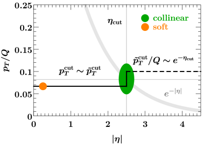
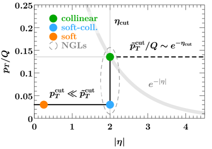
Refer to caption
Refer to caption
Refer to caption
Refer to caption
Figure -1133: Illustration of the parametric regimes for a jet veto with a step. Emissions above the black lines are vetoed, and the thick gray line corresponds to pT/Q=e|η|subscript𝑝𝑇𝑄superscript𝑒𝜂p_{T}/Q=e^{-\lvert\eta\rvert}. The colored circles indicate the relevant modes in the effective theory. The regimes in the top row are characterized by p~Tcuteηcutsimilar-tosuperscriptsubscript~𝑝𝑇cutsuperscript𝑒subscript𝜂cut\tilde{p}_{T}^{\rm cut}\sim e^{-\eta_{\rm cut}}, while those in the bottom row have p~Tcuteηcutmuch-less-thansuperscriptsubscript~𝑝𝑇cutsuperscript𝑒subscript𝜂cut\tilde{p}_{T}^{\rm cut}\ll e^{-\eta_{\rm cut}}. The regimes on the left have pTcutp~Tcutsimilar-tosuperscriptsubscript𝑝𝑇cutsuperscriptsubscript~𝑝𝑇cutp_{T}^{\rm cut}\sim\tilde{p}_{T}^{\rm cut}, while those on the right have pTcutp~Tcutmuch-less-thansuperscriptsubscript𝑝𝑇cutsuperscriptsubscript~𝑝𝑇cutp_{T}^{\rm cut}\ll\tilde{p}_{T}^{\rm cut} and involve parametrically large non-global logarithms.

3.2 𝒑𝑻𝐜𝐮𝐭/𝑸𝒑~𝑻𝐜𝐮𝐭/𝑸𝒆𝜼𝐜𝐮𝐭similar-tosuperscriptsubscript𝒑𝑻𝐜𝐮𝐭𝑸superscriptsubscriptbold-~𝒑𝑻𝐜𝐮𝐭𝑸similar-tosuperscript𝒆subscript𝜼𝐜𝐮𝐭p_{T}^{\rm cut}/Q\sim\tilde{p}_{T}^{\rm cut}/Q\sim e^{-\eta_{\rm cut}} (collinear step)

We first note that the hierarchy pTcut/Qeηcutp~Tcut/Qsimilar-tosuperscriptsubscript𝑝𝑇cut𝑄superscript𝑒subscript𝜂cutmuch-less-thansuperscriptsubscript~𝑝𝑇cut𝑄p_{T}^{\rm cut}/Q\sim e^{-\eta_{\rm cut}}\ll\tilde{p}_{T}^{\rm cut}/Q is effectively equivalent to the case without any jet veto beyond ηcutsubscript𝜂cut\eta_{\rm cut} (regime 2 in section 2.3). Since collinear emissions with |η|>ηcut𝜂subscript𝜂cut\lvert\eta\rvert>\eta_{\rm cut} cannot resolve the loose veto at p~Tcutsuperscriptsubscript~𝑝𝑇cut\tilde{p}_{T}^{\rm cut}, its effect is suppressed by 1/p~Tcut1superscriptsubscript~𝑝𝑇cut1/\tilde{p}_{T}^{\rm cut} and vanishes for p~Tcutsuperscriptsubscript~𝑝𝑇cut\tilde{p}_{T}^{\rm cut}\to\infty.

The first nontrivial hierarchy is pTcut/Qp~Tcut/Qeηcutsimilar-tosuperscriptsubscript𝑝𝑇cut𝑄superscriptsubscript~𝑝𝑇cut𝑄similar-tosuperscript𝑒subscript𝜂cutp_{T}^{\rm cut}/Q\sim\tilde{p}_{T}^{\rm cut}/Q\sim e^{-\eta_{\rm cut}}, illustrated in the top left panel of figure -1133. In this regime, the required modes are the same as in regime 2 in section 2.3. The collinear radiation resolves the step at ηcutsubscript𝜂cut\eta_{\rm cut} while soft emissions are insensitive to it, leading to a generalization of eq. (2.3),

σ0(pTcut,p~Tcut,ηcut,R,Φ)subscript𝜎0superscriptsubscript𝑝𝑇cutsuperscriptsubscript~𝑝𝑇cutsubscript𝜂cut𝑅Φ\displaystyle\sigma_{0}(p_{T}^{\rm cut},\tilde{p}_{T}^{\rm cut},\eta_{\rm cut},R,\Phi) =Hκ(Φ,μ)absentsubscript𝐻𝜅Φ𝜇\displaystyle=H_{\kappa}(\Phi,\mu)\,
×Ba(pTcut,p~Tcut,ηcut,R,ωa,μ,ν)Bb(pTcut,p~Tcut,ηcut,R,ωb,μ,ν)absentsubscript𝐵𝑎superscriptsubscript𝑝𝑇cutsuperscriptsubscript~𝑝𝑇cutsubscript𝜂cut𝑅subscript𝜔𝑎𝜇𝜈subscript𝐵𝑏superscriptsubscript𝑝𝑇cutsuperscriptsubscript~𝑝𝑇cutsubscript𝜂cut𝑅subscript𝜔𝑏𝜇𝜈\displaystyle\quad\times B_{a}(p_{T}^{\rm cut},\tilde{p}_{T}^{\rm cut},\eta_{\rm cut},R,\omega_{a},\mu,\nu)\,B_{b}(p_{T}^{\rm cut},\tilde{p}_{T}^{\rm cut},\eta_{\rm cut},R,\omega_{b},\mu,\nu)\,
×Sκ(pTcut,R,μ,ν)[1+𝒪(pTcutQ,p~TcutQ,eηcut,R2)],absentsubscript𝑆𝜅superscriptsubscript𝑝𝑇cut𝑅𝜇𝜈delimited-[]1𝒪superscriptsubscript𝑝𝑇cut𝑄superscriptsubscript~𝑝𝑇cut𝑄superscript𝑒subscript𝜂cutsuperscript𝑅2\displaystyle\quad\times S_{\kappa}(p_{T}^{\rm cut},R,\mu,\nu)\biggl{[}1+\mathcal{O}\Bigl{(}\frac{p_{T}^{\rm cut}}{Q},\frac{\tilde{p}_{T}^{\rm cut}}{Q},e^{-\eta_{\rm cut}},R^{2}\Bigr{)}\biggr{]}\,, (3.2)

with the beam functions now additionally depending on p~Tcutsuperscriptsubscript~𝑝𝑇cut\tilde{p}_{T}^{\rm cut}. In analogy to eq. (2.16) we write the modified beam function matching coefficients as

ij(pTcut,p~Tcut,ηcut,R,ω,z,μ,ν)subscript𝑖𝑗superscriptsubscript𝑝𝑇cutsuperscriptsubscript~𝑝𝑇cutsubscript𝜂cut𝑅𝜔𝑧𝜇𝜈\displaystyle\mathcal{I}_{ij}(p_{T}^{\rm cut},\tilde{p}_{T}^{\rm cut},\eta_{\rm cut},R,\omega,z,\mu,\nu) =ij(pTcut,R,ω,z,μ,ν)+Δij(pTcut,p~Tcut,ηcut,R,ω,z,μ,ν).absentsubscript𝑖𝑗superscriptsubscript𝑝𝑇cut𝑅𝜔𝑧𝜇𝜈Δsubscript𝑖𝑗superscriptsubscript𝑝𝑇cutsuperscriptsubscript~𝑝𝑇cutsubscript𝜂cut𝑅𝜔𝑧𝜇𝜈\displaystyle=\mathcal{I}_{ij}(p_{T}^{\rm cut},R,\omega,z,\mu,\nu)+\Delta\mathcal{I}_{ij}(p_{T}^{\rm cut},\tilde{p}_{T}^{\rm cut},\eta_{\rm cut},R,\omega,z,\mu,\nu)\,. (3.3)

The first term on the right-hand side is again the matching coefficient for a single veto at pTcutsuperscriptsubscript𝑝𝑇cutp_{T}^{\rm cut} without any rapidity dependence. The second term is the correction due to the step in the jet veto at |η|=ηcut𝜂subscript𝜂cut\lvert\eta\rvert=\eta_{\rm cut}, which vanishes for pTcut=p~Tcutsuperscriptsubscript𝑝𝑇cutsuperscriptsubscript~𝑝𝑇cutp_{T}^{\rm cut}=\tilde{p}_{T}^{\rm cut}. The correction is again renormalized according to eq. (2.3), which as before follows from RG consistency. In particular, its two-loop structure predicted by the RGE is the same as in eq. (2.3), where the finite terms now depend on two dimensionless ratios,

ζcut=ωeηcutpTcut,ζ~cut=ωeηcutp~Tcut.formulae-sequencesubscript𝜁cut𝜔superscript𝑒subscript𝜂cutsuperscriptsubscript𝑝𝑇cutsubscript~𝜁cut𝜔superscript𝑒subscript𝜂cutsuperscriptsubscript~𝑝𝑇cut\zeta_{\rm cut}=\frac{\omega e^{-\eta_{\rm cut}}}{p_{T}^{\rm cut}}\,,\qquad\tilde{\zeta}_{\rm cut}=\frac{\omega e^{-\eta_{\rm cut}}}{\tilde{p}_{T}^{\rm cut}}\,. (3.4)

The one-loop and lnR𝑅\ln R enhanced two-loop finite terms in ΔijΔsubscript𝑖𝑗\Delta\mathcal{I}_{ij} can be written in terms of the results in eqs. (2.25) and (2.27) as

ΔIij(1)(ζcut,ζ~cut,z)Δsubscriptsuperscript𝐼1𝑖𝑗subscript𝜁cutsubscript~𝜁cut𝑧\displaystyle\Delta I^{(1)}_{ij}(\zeta_{\rm cut},\tilde{\zeta}_{\rm cut},z) =ΔIij(1)(ζcut,z)ΔIij(1)(ζ~cut,z),absentΔsubscriptsuperscript𝐼1𝑖𝑗subscript𝜁cut𝑧Δsubscriptsuperscript𝐼1𝑖𝑗subscript~𝜁cut𝑧\displaystyle=\Delta I^{(1)}_{ij}(\zeta_{\rm cut},z)-\Delta I^{(1)}_{ij}(\tilde{\zeta}_{\rm cut},z)\,,
ΔIij(2)(ζcut,ζ~cut,R,z)Δsubscriptsuperscript𝐼2𝑖𝑗subscript𝜁cutsubscript~𝜁cut𝑅𝑧\displaystyle\Delta I^{(2)}_{ij}(\zeta_{\rm cut},\tilde{\zeta}_{\rm cut},R,z) =lnR[ΔIij(2,lnR)(ζcut,z)ΔIij(2,lnR)(ζ~cut,z)],absent𝑅delimited-[]Δsubscriptsuperscript𝐼2𝑅𝑖𝑗subscript𝜁cut𝑧Δsubscriptsuperscript𝐼2𝑅𝑖𝑗subscript~𝜁cut𝑧\displaystyle=\ln R\,\Bigl{[}\Delta I^{(2,\ln R)}_{ij}(\zeta_{\rm cut},z)-\Delta I^{(2,\ln R)}_{ij}(\tilde{\zeta}_{\rm cut},z)\Bigr{]}\,,
+ΔIij(2,c)(ζcut,ζ~cut,z)+𝒪(R2),Δsubscriptsuperscript𝐼2𝑐𝑖𝑗subscript𝜁cutsubscript~𝜁cut𝑧𝒪superscript𝑅2\displaystyle\quad+\Delta I^{(2,c)}_{ij}(\zeta_{\rm cut},\tilde{\zeta}_{\rm cut},z)+\mathcal{O}(R^{2})\,, (3.5)

since for a single (primary) nasubscript𝑛𝑎n_{a}-collinear emission at (η,pT)𝜂subscript𝑝𝑇(\eta,p_{T}) the measurement function for the step correction can be rewritten as

θ(ηηcut)[θ(p~TcutpT)θ(pTcutpT)]𝜃𝜂subscript𝜂cutdelimited-[]𝜃superscriptsubscript~𝑝𝑇cutsubscript𝑝𝑇𝜃superscriptsubscript𝑝𝑇cutsubscript𝑝𝑇\displaystyle\theta(\eta-\eta_{\rm cut})\bigl{[}\theta(\tilde{p}_{T}^{\rm cut}-p_{T})-\theta(p_{T}^{\rm cut}-p_{T})\bigr{]}
=θ(ηηcut)θ(pTpTcut)θ(ηηcut)θ(pTp~Tcut).absent𝜃𝜂subscript𝜂cut𝜃subscript𝑝𝑇superscriptsubscript𝑝𝑇cut𝜃𝜂subscript𝜂cut𝜃subscript𝑝𝑇superscriptsubscript~𝑝𝑇cut\displaystyle\qquad=\theta(\eta-\eta_{\rm cut})\,\theta(p_{T}-p_{T}^{\rm cut})-\theta(\eta-\eta_{\rm cut})\,\theta(p_{T}-\tilde{p}_{T}^{\rm cut})\,. (3.6)

Due to the presence of correlated emissions with rapidities smaller and larger than ηcutsubscript𝜂cut\eta_{\rm cut} at two loops, this decomposition no longer applies for the full two-loop finite term ΔIij(2,c)Δsubscriptsuperscript𝐼2𝑐𝑖𝑗\Delta I^{(2,c)}_{ij}, which therefore needs to be determined separately.

This regime is free of large nonglobal logarithms and is of direct phenomenological interest. The parametric assumptions are satisfied e.g. for high-mass searches, Q300GeVgreater-than-or-equivalent-to𝑄300GeVQ\gtrsim 300\,\mathrm{GeV}, a realistic rapidity cut ηcut=2.5subscript𝜂cut2.5\eta_{\rm cut}=2.5, and veto parameters pTcut=25GeVsuperscriptsubscript𝑝𝑇cut25GeVp_{T}^{\rm cut}=25\,\mathrm{GeV}, p~Tcut=50GeVsuperscriptsubscript~𝑝𝑇cut50GeV\tilde{p}_{T}^{\rm cut}=50\,\mathrm{GeV}, which clearly warrant resummation of logarithms of pTcut/Qp~Tcut/Qeηcutsimilar-tosuperscriptsubscript𝑝𝑇cut𝑄superscriptsubscript~𝑝𝑇cut𝑄similar-tosuperscript𝑒subscript𝜂cutp_{T}^{\rm cut}/Q\sim\tilde{p}_{T}^{\rm cut}/Q\sim e^{-\eta_{\rm cut}}. Evolving the beam function from μBpTcutp~TcutQeηcutsimilar-tosubscript𝜇𝐵superscriptsubscript𝑝𝑇cutsimilar-tosuperscriptsubscript~𝑝𝑇cutsimilar-to𝑄superscript𝑒subscript𝜂cut\mu_{B}\sim p_{T}^{\rm cut}\sim\tilde{p}_{T}^{\rm cut}\sim Qe^{-\eta_{\rm cut}} to μHQsimilar-tosubscript𝜇𝐻𝑄\mu_{H}\sim Q achieves this resummation for all of the above large ratios in the cross section, while the full (logarithmic and nonlogarithmic) dependence on all of the 𝒪(1)𝒪1\mathcal{O}(1) ratios pTcut/p~Tcutsuperscriptsubscript𝑝𝑇cutsuperscriptsubscript~𝑝𝑇cutp_{T}^{\rm cut}/\tilde{p}_{T}^{\rm cut}, Qeηcut/pTcut𝑄superscript𝑒subscript𝜂cutsuperscriptsubscript𝑝𝑇cutQe^{-\eta_{\rm cut}}/p_{T}^{\rm cut}, and Qeηcut/p~Tcut𝑄superscript𝑒subscript𝜂cutsuperscriptsubscript~𝑝𝑇cutQe^{-\eta_{\rm cut}}/\tilde{p}_{T}^{\rm cut} is included at fixed order via the beam function boundary condition.

Numerical validation.
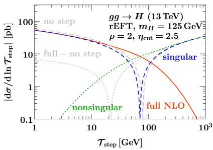
Refer to caption
Refer to caption
Figure -1132: Comparison of singular and nonsingular contributions to the fixed 𝒪(αs)𝒪subscript𝛼𝑠\mathcal{O}(\alpha_{s}) (LO1) 𝒯stepsubscript𝒯step{\mathcal{T}}_{\mathrm{step}} spectrum with a step at ηcut=2.5subscript𝜂cut2.5\eta_{\rm cut}=2.5 and ρ=p~Tcut/pTcut=2𝜌superscriptsubscript~𝑝𝑇cutsuperscriptsubscript𝑝𝑇cut2\rho=\tilde{p}_{T}^{\rm cut}/p_{T}^{\rm cut}=2 for ggH𝑔𝑔𝐻gg\to H (left) and Drell-Yan at Q=mZ𝑄subscript𝑚𝑍Q=m_{Z} (right). The orange solid lines show the full results, the dashed blue lines the singular result that accounts for the jet veto step at ηcutsubscript𝜂cut\eta_{\rm cut} in the beam function, and the dotted green lines their difference. The dashed and dotted gray lines show the corresponding results without taking into account the step in the jet veto, which do not describe the singular behavior of the full cross section.

We now check that the factorized 0-jet cross section in eq. (3.2) reproduces the singular limit of full QCD. For this purpose, we construct an observable that simultaneously forces pTcut0superscriptsubscript𝑝𝑇cut0p_{T}^{\rm cut}\to 0 and p~Tcut0superscriptsubscript~𝑝𝑇cut0\tilde{p}_{T}^{\rm cut}\to 0 as it approaches its singular limit. Following the rapidity-dependent jet vetoes in ref. [16], we define

𝒯step=maxkjets|pT,k|fstep(ηk),fstep(η)={1ρ,|η|>ηcut,1,|η|<ηcut,formulae-sequencesubscript𝒯stepsubscript𝑘jetssubscript𝑝𝑇𝑘subscript𝑓stepsubscript𝜂𝑘subscript𝑓step𝜂cases1𝜌𝜂subscript𝜂cut1𝜂subscript𝜂cut{\mathcal{T}}_{\mathrm{step}}=\max_{k\in\text{jets}}\lvert\vec{p}_{T,k}\rvert f_{\mathrm{step}}(\eta_{k})\,,\qquad f_{\mathrm{step}}(\eta)=\begin{cases}\frac{1}{\rho},\,&\lvert\eta\rvert>\eta_{\rm cut}\,,\\ 1,\,&\lvert\eta\rvert<\eta_{\rm cut}\,,\end{cases} (3.7)

i.e., we can express the step veto by ordering the jets with respect to their weighted transverse momenta, where for |η|>ηcut𝜂subscript𝜂cut\lvert\eta\rvert>\eta_{\rm cut} the corresponding step weight function fstep(η)subscript𝑓step𝜂f_{\mathrm{step}}(\eta) is given by the ratio of veto parameters,

ρp~TcutpTcut>1.𝜌superscriptsubscript~𝑝𝑇cutsuperscriptsubscript𝑝𝑇cut1\rho\equiv\frac{\tilde{p}_{T}^{\rm cut}}{p_{T}^{\rm cut}}>1\,. (3.8)

The differential spectrum in 𝒯stepsubscript𝒯step{\mathcal{T}}_{\mathrm{step}} is then related to the jet-vetoed cross section with a step by the relation

σ0(pTcut,ρpTcut,ηcut,R)=0pTcutd𝒯stepdσ(ρ,ηcut,R)d𝒯step.subscript𝜎0superscriptsubscript𝑝𝑇cut𝜌superscriptsubscript𝑝𝑇cutsubscript𝜂cut𝑅superscriptsubscript0superscriptsubscript𝑝𝑇cutdifferential-dsubscript𝒯stepd𝜎𝜌subscript𝜂cut𝑅dsubscript𝒯step\sigma_{0}(p_{T}^{\rm cut},\,\rho\,p_{T}^{\rm cut},\,\eta_{\rm cut},R)=\int_{0}^{p_{T}^{\rm cut}}\!\mathrm{d}{\mathcal{T}}_{\mathrm{step}}\,\frac{\mathrm{d}\sigma(\rho,\eta_{\rm cut},R)}{\mathrm{d}{\mathcal{T}}_{\mathrm{step}}}\,. (3.9)

In figure -1132 we compare dσ(ρ,ηcut)/d𝒯stepd𝜎𝜌subscript𝜂cutdsubscript𝒯step\mathrm{d}\sigma(\rho,\eta_{\rm cut})/\mathrm{d}{\mathcal{T}}_{\mathrm{step}} at fixed 𝒪(αs)𝒪subscript𝛼𝑠\mathcal{O}(\alpha_{s}) in full QCD to the singular spectrum predicted by eq. (3.2) as well as the standard factorization eq. (2.2) without a step for ggH𝑔𝑔𝐻gg\to H (left panel) and Drell-Yan at the Z𝑍Z pole (right panel). The singular result using the full p~Tcutsuperscriptsubscript~𝑝𝑇cut\tilde{p}_{T}^{\rm cut} and ηcutsubscript𝜂cut\eta_{\rm cut} dependent beam functions (dashed blue) correctly reproduces the singular behavior of full QCD (solid orange) in the limit 𝒯step0subscript𝒯step0{\mathcal{T}}_{\mathrm{step}}\to 0, with the difference to the full QCD spectrum (dotted green) vanishing like a power in 𝒯stepsubscript𝒯step{\mathcal{T}}_{\mathrm{step}} as it should. On the other hand, the standard factorization without step (dashed gray) does not reproduce the correct singular behavior of full QCD, with the difference (dotted gray) diverging for 𝒯step0subscript𝒯step0{\mathcal{T}}_{\mathrm{step}}\to 0. Note that the mismatch here is reduced compared to the p~Tcut=superscriptsubscript~𝑝𝑇cut\tilde{p}_{T}^{\rm cut}=\infty case shown in figures -1136 and -1135, owing to the larger phase space available to unconstrained radiation at |η|>ηcut𝜂subscript𝜂cut\lvert\eta\rvert>\eta_{\rm cut} for p~Tcut=superscriptsubscript~𝑝𝑇cut\tilde{p}_{T}^{\rm cut}=\infty.

3.3 𝒑𝑻𝐜𝐮𝐭/𝑸𝒑~𝑻𝐜𝐮𝐭/𝑸𝒆𝜼𝐜𝐮𝐭much-less-thansuperscriptsubscript𝒑𝑻𝐜𝐮𝐭𝑸superscriptsubscriptbold-~𝒑𝑻𝐜𝐮𝐭𝑸similar-tosuperscript𝒆subscript𝜼𝐜𝐮𝐭p_{T}^{\rm cut}/Q\ll\tilde{p}_{T}^{\rm cut}/Q\sim e^{-\eta_{\rm cut}} (collinear NGLs)

This regime is a direct extension of regime 3 without a step in section 2.4. For eηcutp~Tcut/Qmuch-less-thansuperscript𝑒subscript𝜂cutsuperscriptsubscript~𝑝𝑇cut𝑄e^{-\eta_{\rm cut}}\ll\tilde{p}_{T}^{\rm cut}/Q, the effect of p~Tcutsuperscriptsubscript~𝑝𝑇cut\tilde{p}_{T}^{\rm cut} is again suppressed by 1/p~Tcut1superscriptsubscript~𝑝𝑇cut1/\tilde{p}_{T}^{\rm cut} and vanishes for p~Tcutsuperscriptsubscript~𝑝𝑇cut\tilde{p}_{T}^{\rm cut}\to\infty, yielding the same result as in section 2.4. The nontrivial new hierarchy is pTcut/Qp~Tcut/Qeηcutmuch-less-thansuperscriptsubscript𝑝𝑇cut𝑄superscriptsubscript~𝑝𝑇cut𝑄similar-tosuperscript𝑒subscript𝜂cutp_{T}^{\rm cut}/Q\ll\tilde{p}_{T}^{\rm cut}/Q\sim e^{-\eta_{\rm cut}}, shown in the top right panel of figure -1133. In this regime, the mode setup is as in section 2.4. However, the collinear modes are now additionally constrained for |η|>ηcut𝜂subscript𝜂cut\lvert\eta\rvert>\eta_{\rm cut} by the jet veto at p~Tcutsuperscriptsubscript~𝑝𝑇cut\tilde{p}_{T}^{\rm cut}, making them sensitive to both p~Tcutsuperscriptsubscript~𝑝𝑇cut\tilde{p}_{T}^{\rm cut} and the kinematic scale Qeηcut𝑄superscript𝑒subscript𝜂cutQe^{-\eta_{\rm cut}}. This leads to a modification of the overall initial-state collinear functions in eqs. (2.4) and (2.36) by

i(pTcut,p~Tcut,ηcut,R,ω,μ,ν)subscript𝑖superscriptsubscript𝑝𝑇cutsuperscriptsubscript~𝑝𝑇cutsubscript𝜂cut𝑅𝜔𝜇𝜈\displaystyle\mathcal{B}_{i}(p_{T}^{\rm cut},\tilde{p}_{T}^{\rm cut},\eta_{\rm cut},R,\omega,\mu,\nu) =Bi(cut)(p~Tcut,ηcut,R,ω,μ)𝒮i(cut)(pTcut,ηcut,R,μ,ν)absentsubscriptsuperscript𝐵cut𝑖superscriptsubscript~𝑝𝑇cutsubscript𝜂cut𝑅𝜔𝜇subscriptsuperscript𝒮cut𝑖superscriptsubscript𝑝𝑇cutsubscript𝜂cut𝑅𝜇𝜈\displaystyle=B^{(\rm cut)}_{i}(\tilde{p}_{T}^{\rm cut},\eta_{\rm cut},R,\omega,\mu)\,\mathcal{S}^{(\rm cut)}_{i}(p_{T}^{\rm cut},\eta_{\rm cut},R,\mu,\nu)
×[1+i(NG)(pTcutωeηcut,pTcutp~Tcut,ω,R)].absentdelimited-[]1subscriptsuperscriptNG𝑖superscriptsubscript𝑝𝑇cut𝜔superscript𝑒subscript𝜂cutsuperscriptsubscript𝑝𝑇cutsuperscriptsubscript~𝑝𝑇cut𝜔𝑅\displaystyle\quad\times\biggl{[}1+\mathcal{B}^{\rm(NG)}_{i}\Bigl{(}\frac{p_{T}^{\rm cut}}{\omega e^{-\eta_{\rm cut}}},\frac{p_{T}^{\rm cut}}{\tilde{p}_{T}^{\rm cut}},\omega,R\Bigr{)}\biggr{]}\,. (3.10)

Here 𝒮i(cut)subscriptsuperscript𝒮cut𝑖\mathcal{S}^{(\rm cut)}_{i} is the same soft-collinear function as in eq. (2.4). By RG consistency the functions Bi(cut)subscriptsuperscript𝐵cut𝑖B^{(\rm cut)}_{i} have the same renormalization as those in eq. (2.4), i.e., the additional dependence on p~Tcutsuperscriptsubscript~𝑝𝑇cut\tilde{p}_{T}^{\rm cut} does not change their renormalization. The associated matching coefficients at one loop are given by subtracting the correction term ΔIij(1)Δsuperscriptsubscript𝐼𝑖𝑗1\Delta I_{ij}^{(1)} in eq. (2.25), which accounts for an n𝑛n-collinear emission with η>ηcut𝜂subscript𝜂cut\eta>\eta_{\rm cut} and pT>p~Tcutsubscript𝑝𝑇superscriptsubscript~𝑝𝑇cutp_{T}>\tilde{p}_{T}^{\rm cut}, from the coefficient ij(cut)subscriptsuperscriptcut𝑖𝑗\mathcal{I}^{({\rm cut})}_{ij} in eq. (2.4), which accounts for an n𝑛n-collinear emission with η>ηcut𝜂subscript𝜂cut\eta>\eta_{\rm cut} without constraints from a jet veto, such that

ij(cut)(p~Tcut,ηcut,R,ω,z,μ)=ij(cut)(ηcut,ω,z,μ)αs(μ)4πΔIij(1)(ωeηcutp~Tcut,z,R)+𝒪(αs2).subscriptsuperscriptcut𝑖𝑗superscriptsubscript~𝑝𝑇cutsubscript𝜂cut𝑅𝜔𝑧𝜇subscriptsuperscriptcut𝑖𝑗subscript𝜂cut𝜔𝑧𝜇subscript𝛼𝑠𝜇4𝜋Δsubscriptsuperscript𝐼1𝑖𝑗𝜔superscript𝑒subscript𝜂cutsuperscriptsubscript~𝑝𝑇cut𝑧𝑅𝒪superscriptsubscript𝛼𝑠2\displaystyle\mathcal{I}^{({\rm cut})}_{ij}(\tilde{p}_{T}^{\rm cut},\eta_{\rm cut},R,\omega,z,\mu)=\mathcal{I}^{({\rm cut})}_{ij}(\eta_{\rm cut},\omega,z,\mu)-\frac{\alpha_{s}(\mu)}{4\pi}\Delta I^{(1)}_{ij}\Bigl{(}\frac{\omega e^{-\eta_{\rm cut}}}{\tilde{p}_{T}^{\rm cut}},z,R\Bigr{)}+\mathcal{O}(\alpha_{s}^{2})\,. (3.11)

The i(NG)subscriptsuperscriptNG𝑖\mathcal{B}^{\rm(NG)}_{i} term in eq. (3.3) contains nonglobal logarithms of pTcut/p~TcutpTcut/Qeηcutsimilar-tosuperscriptsubscript𝑝𝑇cutsuperscriptsubscript~𝑝𝑇cutsuperscriptsubscript𝑝𝑇cut𝑄superscript𝑒subscript𝜂cutp_{T}^{\rm cut}/\tilde{p}_{T}^{\rm cut}\sim p_{T}^{\rm cut}/Qe^{-\eta_{\rm cut}}.

3.4 𝒑𝑻𝐜𝐮𝐭/𝑸𝒑~𝑻𝐜𝐮𝐭/𝑸𝒆𝜼𝐜𝐮𝐭similar-tosuperscriptsubscript𝒑𝑻𝐜𝐮𝐭𝑸superscriptsubscriptbold-~𝒑𝑻𝐜𝐮𝐭𝑸much-less-thansuperscript𝒆subscript𝜼𝐜𝐮𝐭p_{T}^{\rm cut}/Q\sim\tilde{p}_{T}^{\rm cut}/Q\ll e^{-\eta_{\rm cut}} (soft-collinear step)

In this regime (bottom left panel of figure -1133), the mode setup in section 2.2 is extended by soft-collinear modes that resolve the step in the jet veto at ηcutsubscript𝜂cut\eta_{\rm cut},

na-soft-collinear:subscript𝑛𝑎-soft-collinear:\displaystyle n_{a}\text{-soft-collinear:} pμpTcut(eηcut,eηcut,1)p~Tcut(eηcut,eηcut,1),similar-tosuperscript𝑝𝜇superscriptsubscript𝑝𝑇cutsuperscript𝑒subscript𝜂cutsuperscript𝑒subscript𝜂cut1similar-tosuperscriptsubscript~𝑝𝑇cutsuperscript𝑒subscript𝜂cutsuperscript𝑒subscript𝜂cut1\displaystyle\quad p^{\mu}\sim p_{T}^{\rm cut}(e^{-\eta_{\rm cut}},e^{\eta_{\rm cut}},1)\sim\tilde{p}_{T}^{\rm cut}(e^{-\eta_{\rm cut}},e^{\eta_{\rm cut}},1)\,,
nb-soft-collinear:subscript𝑛𝑏-soft-collinear:\displaystyle n_{b}\text{-soft-collinear:} pμpTcut(eηcut,eηcut,1)p~Tcut(eηcut,eηcut,1).similar-tosuperscript𝑝𝜇superscriptsubscript𝑝𝑇cutsuperscript𝑒subscript𝜂cutsuperscript𝑒subscript𝜂cut1similar-tosuperscriptsubscript~𝑝𝑇cutsuperscript𝑒subscript𝜂cutsuperscript𝑒subscript𝜂cut1\displaystyle\quad p^{\mu}\sim p_{T}^{\rm cut}(e^{\eta_{\rm cut}},e^{-\eta_{\rm cut}},1)\sim\tilde{p}_{T}^{\rm cut}(e^{\eta_{\rm cut}},e^{-\eta_{\rm cut}},1)\,. (3.12)

At the same time, the collinear modes only see the jet veto at p~Tcutsuperscriptsubscript~𝑝𝑇cut\tilde{p}_{T}^{\rm cut}, while the soft modes only see the veto at pTcutsuperscriptsubscript𝑝𝑇cutp_{T}^{\rm cut}. This yields the factorized cross section

σ0(pTcut,p~Tcut,ηcut,R,Φ)subscript𝜎0superscriptsubscript𝑝𝑇cutsuperscriptsubscript~𝑝𝑇cutsubscript𝜂cut𝑅Φ\displaystyle\sigma_{0}(p_{T}^{\rm cut},\tilde{p}_{T}^{\rm cut},\eta_{\rm cut},R,\Phi) =Hκ(Φ,μ)Ba(p~Tcut,R,ω,μ,ν)Bb(p~Tcut,R,ω,μ,ν)Sκ(pTcut,μ,ν)absentsubscript𝐻𝜅Φ𝜇subscript𝐵𝑎superscriptsubscript~𝑝𝑇cut𝑅𝜔𝜇𝜈subscript𝐵𝑏superscriptsubscript~𝑝𝑇cut𝑅𝜔𝜇𝜈subscript𝑆𝜅superscriptsubscript𝑝𝑇cut𝜇𝜈\displaystyle=H_{\kappa}(\Phi,\mu)\,B_{a}(\tilde{p}_{T}^{\rm cut},R,\omega,\mu,\nu)\,B_{b}(\tilde{p}_{T}^{\rm cut},R,\omega,\mu,\nu)\,S_{\kappa}(p_{T}^{\rm cut},\mu,\nu)
×𝒮a(pTcut,p~Tcut,ηcut,R,μ,ν)𝒮b(pTcut,p~Tcut,ηcut,R,μ,ν)absentsubscript𝒮𝑎superscriptsubscript𝑝𝑇cutsuperscriptsubscript~𝑝𝑇cutsubscript𝜂cut𝑅𝜇𝜈subscript𝒮𝑏superscriptsubscript𝑝𝑇cutsuperscriptsubscript~𝑝𝑇cutsubscript𝜂cut𝑅𝜇𝜈\displaystyle\quad\times\mathcal{S}_{a}(p_{T}^{\rm cut},\tilde{p}_{T}^{\rm cut},\eta_{\rm cut},R,\mu,\nu)\,\mathcal{S}_{b}(p_{T}^{\rm cut},\tilde{p}_{T}^{\rm cut},\eta_{\rm cut},R,\mu,\nu)
×[1+𝒪(pTcutQ,p~TcutQ,pTcutQeηcut,p~TcutQeηcut,R2)].absentdelimited-[]1𝒪superscriptsubscript𝑝𝑇cut𝑄superscriptsubscript~𝑝𝑇cut𝑄superscriptsubscript𝑝𝑇cut𝑄superscript𝑒subscript𝜂cutsuperscriptsubscript~𝑝𝑇cut𝑄superscript𝑒subscript𝜂cutsuperscript𝑅2\displaystyle\quad\times\biggl{[}1+\mathcal{O}\Bigl{(}\frac{p_{T}^{\rm cut}}{Q},\frac{\tilde{p}_{T}^{\rm cut}}{Q},\frac{p_{T}^{\rm cut}}{Qe^{-\eta_{\rm cut}}},\frac{\tilde{p}_{T}^{\rm cut}}{Qe^{-\eta_{\rm cut}}},R^{2}\Bigr{)}\biggr{]}\,. (3.13)

The soft-collinear function 𝒮isubscript𝒮𝑖\mathcal{S}_{i} encodes the actual step at ηcutsubscript𝜂cut\eta_{\rm cut} and is defined by the measurement eq. (3.1). For p~Tcut=pTcutsuperscriptsubscript~𝑝𝑇cutsuperscriptsubscript𝑝𝑇cut\tilde{p}_{T}^{\rm cut}=p_{T}^{\rm cut} there is no step in the jet veto and 𝒮isubscript𝒮𝑖\mathcal{S}_{i} has to vanish. The RG consistency of the cross section implies that its μ𝜇\mu anomalous dimension vanishes in general, while its resummed ν𝜈\nu anomalous dimension is given by

γν,𝒮i(pTcut,p~Tcut,R)=2ηΓi(pTcut,p~Tcut)+12{γνi[αs(p~Tcut),R]γνi[αs(pTcut),R]}.subscriptsuperscript𝛾𝑖𝜈𝒮superscriptsubscript𝑝𝑇cutsuperscriptsubscript~𝑝𝑇cut𝑅2superscriptsubscript𝜂Γ𝑖superscriptsubscript𝑝𝑇cutsuperscriptsubscript~𝑝𝑇cut12superscriptsubscript𝛾𝜈𝑖subscript𝛼𝑠superscriptsubscript~𝑝𝑇cut𝑅superscriptsubscript𝛾𝜈𝑖subscript𝛼𝑠superscriptsubscript𝑝𝑇cut𝑅\displaystyle\gamma^{i}_{\nu,\mathcal{S}}(p_{T}^{\rm cut},\tilde{p}_{T}^{\rm cut},R)=2\eta_{\Gamma}^{i}(p_{T}^{\rm cut},\tilde{p}_{T}^{\rm cut})+\frac{1}{2}\Bigl{\{}\gamma_{\nu}^{i}[\alpha_{s}(\tilde{p}_{T}^{\rm cut}),R]-\gamma_{\nu}^{i}[\alpha_{s}(p_{T}^{\rm cut}),R]\Bigr{\}}\,. (3.14)

It does not depend on μ𝜇\mu at all, as required by exact path independence in the (μ,ν)𝜇𝜈(\mu,\nu) plane. Note that the beam functions in eq. (3.4) depend on p~Tcutsuperscriptsubscript~𝑝𝑇cut\tilde{p}_{T}^{\rm cut} (rather than pTcutsuperscriptsubscript𝑝𝑇cutp_{T}^{\rm cut}) because collinear radiation is too forward to be constrained by the tighter central veto. This is reflected in the somewhat curious rapidity anomalous dimension of 𝒮isubscript𝒮𝑖\mathcal{S}_{i} in eq. (3.14), which accounts for the mismatch between the logarithms of pTcutsuperscriptsubscript𝑝𝑇cutp_{T}^{\rm cut} and p~Tcutsuperscriptsubscript~𝑝𝑇cut\tilde{p}_{T}^{\rm cut} generated by the soft and beam rapidity evolution, respectively.

Solving eq. (3.14) order by order in αssubscript𝛼𝑠\alpha_{s} we find the following very simple structure of the soft-collinear function through two loops:

𝒮i(pTcut,p~Tcut,ηcut,R,μ,ν)subscript𝒮𝑖superscriptsubscript𝑝𝑇cutsuperscriptsubscript~𝑝𝑇cutsubscript𝜂cut𝑅𝜇𝜈\displaystyle\mathcal{S}_{i}(p_{T}^{\rm cut},\tilde{p}_{T}^{\rm cut},\eta_{\rm cut},R,\mu,\nu) =1+αs(μ)4π[2Γ0ilnρL𝒮ν+𝒮i,1(ρ)]absent1subscript𝛼𝑠𝜇4𝜋delimited-[]2subscriptsuperscriptΓ𝑖0𝜌subscriptsuperscript𝐿𝜈𝒮subscript𝒮𝑖1𝜌\displaystyle=1+\frac{\alpha_{s}(\mu)}{4\pi}\Bigl{[}2\Gamma^{i}_{0}\ln\rho\,L^{\nu}_{\mathcal{S}}+\mathcal{S}_{i,1}(\rho)\Bigr{]} (3.15)
+αs2(μ)(4π)2{2(Γ0i)2ln2ρ(L𝒮ν)2+2lnρL𝒮ν[2L𝒮μβ0Γ0i+Γ0i𝒮i,1(ρ)+Γ1i]\displaystyle\quad+\frac{\alpha_{s}^{2}(\mu)}{(4\pi)^{2}}\Bigl{\{}2(\Gamma^{i}_{0})^{2}\!\ln^{2}\!\!\rho\,(L^{\nu}_{\mathcal{S}})^{2}\!+\!2\ln\rho\,L^{\nu}_{\mathcal{S}}\bigl{[}2L^{\mu}_{\mathcal{S}}\beta_{0}\Gamma^{i}_{0}\!+\!\Gamma^{i}_{0}\mathcal{S}_{i,1}(\rho)\!+\!\Gamma^{i}_{1}\bigr{]}
+2β0L𝒮μ𝒮i,1(ρ)+𝒮i,2(ρ,R)}+𝒪(αs3),\displaystyle\qquad\qquad\qquad+2\beta_{0}L^{\mu}_{\mathcal{S}}\,\mathcal{S}_{i,1}(\rho)+\mathcal{S}_{i,2}(\rho,R)\Bigr{\}}+\mathcal{O}(\alpha_{s}^{3})\,,

where

ρp~TcutpTcut,L𝒮νlnνpTcutp~Tcuteηcut,L𝒮μlnμpTcutp~Tcut.formulae-sequence𝜌superscriptsubscript~𝑝𝑇cutsuperscriptsubscript𝑝𝑇cutformulae-sequencesubscriptsuperscript𝐿𝜈𝒮𝜈superscriptsubscript𝑝𝑇cutsuperscriptsubscript~𝑝𝑇cutsuperscript𝑒subscript𝜂cutsubscriptsuperscript𝐿𝜇𝒮𝜇superscriptsubscript𝑝𝑇cutsuperscriptsubscript~𝑝𝑇cut\rho\equiv\frac{\tilde{p}_{T}^{\rm cut}}{p_{T}^{\rm cut}}\,,\qquad L^{\nu}_{\mathcal{S}}\equiv\ln\frac{\nu}{\sqrt{p_{T}^{\rm cut}\tilde{p}_{T}^{\rm cut}}e^{\eta_{\rm cut}}}\,,\qquad L^{\mu}_{\mathcal{S}}\equiv\ln\frac{\mu}{\sqrt{p_{T}^{\rm cut}\tilde{p}_{T}^{\rm cut}}}\,. (3.16)

It is straightforward to check that the one-loop finite term vanishes (see appendix A.4),

𝒮i,1=0.subscript𝒮𝑖10\mathcal{S}_{i,1}=0\,. (3.17)

The two-loop finite term is a generic function of the dimensionless ratio ρ𝜌\rho and the jet radius parameter R𝑅R, which must satisfy 𝒮i,2(ρ=1,R)=0subscript𝒮𝑖2𝜌1𝑅0\mathcal{S}_{i,2}(\rho=1,R)=0. As usual, we can decompose it according to its R𝑅R dependence as

𝒮i,2(ρ,R)=8CiciiRlnρlnR+𝒮i,2(c)(ρ)+𝒪(R2),subscript𝒮𝑖2𝜌𝑅8subscript𝐶𝑖superscriptsubscript𝑐𝑖𝑖𝑅𝜌𝑅superscriptsubscript𝒮𝑖2𝑐𝜌𝒪superscript𝑅2\mathcal{S}_{i,2}(\rho,R)=-8C_{i}c_{ii}^{R}\,\ln\rho\ln R+\mathcal{S}_{i,2}^{(c)}(\rho)+\mathcal{O}(R^{2})\,, (3.18)

where ciiRsuperscriptsubscript𝑐𝑖𝑖𝑅c_{ii}^{R} is given by eq. (2.3) and Ci=CF(CA)subscript𝐶𝑖subscript𝐶𝐹subscript𝐶𝐴C_{i}=C_{F}\,(C_{A}) for i=q(g)𝑖𝑞𝑔i=q\,(g). The coefficient of lnR𝑅\ln R at this order is completely determined by the R𝑅R dependence of the noncusp rapidity anomalous dimensions in eq. (3.14). The full two-loop finite term 𝒮i,2(ρ,R)subscript𝒮𝑖2𝜌𝑅\mathcal{S}_{i,2}(\rho,R) could readily be obtained numerically using the methods of refs. [62, 63], which would enable the full NNLL resummation.

This regime is again free of nonglobal logarithms and hence can easily be applied to phenomenological studies. It can be used to supplement the EFT setup from section 3.2, which enables the resummation of logarithms of the ratio pTcut/Qp~Tcut/Qsimilar-tosuperscriptsubscript𝑝𝑇cut𝑄superscriptsubscript~𝑝𝑇cut𝑄p_{T}^{\rm cut}/Q\sim\tilde{p}_{T}^{\rm cut}/Q, with an additional resummation of logarithms of the ratio pTcut/Qeηcutp~Tcut/Qeηcutsimilar-tosuperscriptsubscript𝑝𝑇cut𝑄superscript𝑒subscript𝜂cutsuperscriptsubscript~𝑝𝑇cut𝑄superscript𝑒subscript𝜂cutp_{T}^{\rm cut}/Qe^{-\eta_{\rm cut}}\sim\tilde{p}_{T}^{\rm cut}/Qe^{-\eta_{\rm cut}} by choosing the canonical scales

μBsubscript𝜇𝐵\displaystyle\mu_{B} p~Tcut,similar-toabsentsuperscriptsubscript~𝑝𝑇cut\displaystyle\sim\tilde{p}_{T}^{\rm cut}\,,\quad μ𝒮subscript𝜇𝒮\displaystyle\mu_{\mathcal{S}} pTcutp~Tcut,similar-toabsentsuperscriptsubscript𝑝𝑇cutsuperscriptsubscript~𝑝𝑇cut\displaystyle\sim\sqrt{p_{T}^{\rm cut}\tilde{p}_{T}^{\rm cut}}\,,\quad μSsubscript𝜇𝑆\displaystyle\mu_{S} pTcut,similar-toabsentsuperscriptsubscript𝑝𝑇cut\displaystyle\sim p_{T}^{\rm cut}\,,
νBsubscript𝜈𝐵\displaystyle\nu_{B} Q,similar-toabsent𝑄\displaystyle\sim Q\,,\quad ν𝒮subscript𝜈𝒮\displaystyle\nu_{\mathcal{S}} pTcutp~Tcuteηcut,similar-toabsentsuperscriptsubscript𝑝𝑇cutsuperscriptsubscript~𝑝𝑇cutsuperscript𝑒subscript𝜂cut\displaystyle\sim\sqrt{p_{T}^{\rm cut}\tilde{p}_{T}^{\rm cut}}e^{\eta_{\rm cut}}\,,\quad νSsubscript𝜈𝑆\displaystyle\nu_{S} pTcut.similar-toabsentsuperscriptsubscript𝑝𝑇cut\displaystyle\sim p_{T}^{\rm cut}\,. (3.19)

Here, the rapidity evolution between ν𝒮subscript𝜈𝒮\nu_{\mathcal{S}} and νSsubscript𝜈𝑆\nu_{S} is responsible for resumming the large logarithms of eηcutνS/ν𝒮similar-tosuperscript𝑒subscript𝜂cutsubscript𝜈𝑆subscript𝜈𝒮e^{-\eta_{\rm cut}}\sim\nu_{S}/\nu_{\mathcal{S}}.

Numerical Validation.

Refer to caption
Refer to caption
Refer to caption
Refer to caption
Figure -1131: Comparison of the singular contributions to the fixed 𝒪(αs)𝒪subscript𝛼𝑠\mathcal{O}(\alpha_{s}) (LO1) 𝒯stepsubscript𝒯step{\mathcal{T}}_{\mathrm{step}} spectrum for ηcut=2.5subscript𝜂cut2.5\eta_{\rm cut}=2.5 and ρ=2𝜌2\rho=2 for ggH𝑔𝑔𝐻gg\to H (top left), ggX𝑔𝑔𝑋gg\to X (top right), and Drell-Yan at Q=mZ𝑄subscript𝑚𝑍Q=m_{Z} (bottom left) and Q=1TeV𝑄1TeVQ=1\,\mathrm{TeV} (bottom right). The solid orange lines show the singular spectrum for the collinear-step regime and the blue dashed lines the further factorized result in the soft-collinear-step regime. Their difference, shown by the dotted green lines vanishes as a power of 𝒯stepsubscript𝒯step{\mathcal{T}}_{\mathrm{step}}. The vertical lines indicate where the parametric relation 𝒯step/Q=eηcutsubscript𝒯step𝑄superscript𝑒subscript𝜂cut{\mathcal{T}}_{\mathrm{step}}/Q=e^{-\eta_{\rm cut}} is satisfied.

To validate our setup in this regime, we exploit that eq. (3.4) provides a refactorization of the collinear step in eq. (3.2), where

ij(pTcut,p~Tcut,ηcut,R,ω,z,μ,ν)subscript𝑖𝑗superscriptsubscript𝑝𝑇cutsuperscriptsubscript~𝑝𝑇cutsubscript𝜂cut𝑅𝜔𝑧𝜇𝜈\displaystyle\mathcal{I}_{ij}(p_{T}^{\rm cut},\tilde{p}_{T}^{\rm cut},\eta_{\rm cut},R,\omega,z,\mu,\nu) =𝒮i(pTcut,p~Tcut,ηcut,R,μ,ν)ij(pTcut,R,ω,z,μ,ν)absentsubscript𝒮𝑖superscriptsubscript𝑝𝑇cutsuperscriptsubscript~𝑝𝑇cutsubscript𝜂cut𝑅𝜇𝜈subscript𝑖𝑗superscriptsubscript𝑝𝑇cut𝑅𝜔𝑧𝜇𝜈\displaystyle=\mathcal{S}_{i}(p_{T}^{\rm cut},\tilde{p}_{T}^{\rm cut},\eta_{\rm cut},R,\mu,\nu)\,\mathcal{I}_{ij}(p_{T}^{\rm cut},R,\omega,z,\mu,\nu)
×[1+𝒪(pTcutωeηcut,p~Tcutωeηcut,R2)].absentdelimited-[]1𝒪superscriptsubscript𝑝𝑇cut𝜔superscript𝑒subscript𝜂cutsuperscriptsubscript~𝑝𝑇cut𝜔superscript𝑒subscript𝜂cutsuperscript𝑅2\displaystyle\quad\times\biggl{[}1+\mathcal{O}\Bigl{(}\frac{p_{T}^{\rm cut}}{\omega e^{-\eta_{\rm cut}}},\frac{\tilde{p}_{T}^{\rm cut}}{\omega e^{-\eta_{\rm cut}}},R^{2}\Bigr{)}\biggr{]}\,. (3.20)

In particular, eq. (3.4) must reproduce eq. (3.2) up to power corrections in pTcut/Qeηcutsuperscriptsubscript𝑝𝑇cut𝑄superscript𝑒subscript𝜂cutp_{T}^{\rm cut}/Qe^{-\eta_{\rm cut}} and p~Tcut/Qeηcutsuperscriptsubscript~𝑝𝑇cut𝑄superscript𝑒subscript𝜂cut\tilde{p}_{T}^{\rm cut}/Qe^{-\eta_{\rm cut}}. We can test this numerically using the 𝒯stepsubscript𝒯step{\mathcal{T}}_{\mathrm{step}} observable defined in section 3.2, which simultaneously probes both classes of power corrections. In figure -1131, we show the fixed 𝒪(αs)𝒪subscript𝛼𝑠\mathcal{O}(\alpha_{s}) 𝒯stepsubscript𝒯step{\mathcal{T}}_{\mathrm{step}} spectra for the collinear step (solid orange) and soft-collinear step (dashed blue). In all cases their difference (dotted green) vanishes like a power in 𝒯stepsubscript𝒯step{\mathcal{T}}_{\mathrm{step}}.

The additional resummation using the soft-collinear step may be applicable up to values of pTcut=20GeVsuperscriptsubscript𝑝𝑇cut20GeVp_{T}^{\rm cut}=20\,\mathrm{GeV} (pTcut=80GeVsuperscriptsubscript𝑝𝑇cut80GeVp_{T}^{\rm cut}=80\,\mathrm{GeV}) for Q100GeVsimilar-to𝑄100GeVQ\sim 100\,\mathrm{GeV} (Q=1TeV𝑄1TeVQ=1\,\mathrm{TeV}), for the choice of ρ=2,ηcut=2.5formulae-sequence𝜌2subscript𝜂cut2.5\rho=2,\eta_{\rm cut}=2.5 displayed in figure -1131. This can be read off from the relative size of leading-power (soft-collinear step) and subleading power (difference) contributions, which leave some room where resummation in the leading-power cross section can improve the prediction. We find a slightly larger potential resummation region than for the analogous refactorization in the p~Tcut=superscriptsubscript~𝑝𝑇cut\tilde{p}_{T}^{\rm cut}=\infty case, where an earlier onset of the power corrections was observed in figure -1134.

3.5 𝒑𝑻𝐜𝐮𝐭/𝑸𝒑~𝑻𝐜𝐮𝐭/𝑸𝒆𝜼𝐜𝐮𝐭much-less-thansuperscriptsubscript𝒑𝑻𝐜𝐮𝐭𝑸superscriptsubscriptbold-~𝒑𝑻𝐜𝐮𝐭𝑸much-less-thansuperscript𝒆subscript𝜼𝐜𝐮𝐭p_{T}^{\rm cut}/Q\ll\tilde{p}_{T}^{\rm cut}/Q\ll e^{-\eta_{\rm cut}} (soft-collinear NGLs)

For this hierarchy (bottom right panel of figure -1133), two types of soft-collinear modes arise,

na-soft-collinear (pTcut):subscript𝑛𝑎-soft-collinear (pTcut):\displaystyle n_{a}\text{-soft-collinear ($p_{T}^{\rm cut}$):} pμpTcut(eηcut,eηcut,1),similar-tosuperscript𝑝𝜇superscriptsubscript𝑝𝑇cutsuperscript𝑒subscript𝜂cutsuperscript𝑒subscript𝜂cut1\displaystyle\quad p^{\mu}\sim p_{T}^{\rm cut}(e^{-\eta_{\rm cut}},e^{\eta_{\rm cut}},1)\,,
na-soft-collinear (p~Tcut):subscript𝑛𝑎-soft-collinear (p~Tcut):\displaystyle n_{a}\text{-soft-collinear ($\tilde{p}_{T}^{\rm cut}$):} pμp~Tcut(eηcut,eηcut,1),similar-tosuperscript𝑝𝜇superscriptsubscript~𝑝𝑇cutsuperscript𝑒subscript𝜂cutsuperscript𝑒subscript𝜂cut1\displaystyle\quad p^{\mu}\sim\tilde{p}_{T}^{\rm cut}(e^{-\eta_{\rm cut}},e^{\eta_{\rm cut}},1)\,, (3.21)

and analogously for the nbsubscript𝑛𝑏n_{b}-soft-collinear sectors, which are both parametrically distinct from the energetic collinear modes. Compared to the regime pTcutp~TcutQeηcutsimilar-tosuperscriptsubscript𝑝𝑇cutsuperscriptsubscript~𝑝𝑇cutmuch-less-than𝑄superscript𝑒subscript𝜂cutp_{T}^{\rm cut}\sim\tilde{p}_{T}^{\rm cut}\ll Qe^{-\eta_{\rm cut}} there are now parametrically large logarithms ln(pTcut/p~Tcut)superscriptsubscript𝑝𝑇cutsuperscriptsubscript~𝑝𝑇cut\ln(p_{T}^{\rm cut}/\tilde{p}_{T}^{\rm cut}) in the soft-collinear function 𝒮isubscript𝒮𝑖\mathcal{S}_{i} in eq. (3.4). The cross section can be written as in eq. (3.4), where the soft-collinear function is refactorized as

𝒮i(pTcut,p~Tcut,ηcut,R,μ,ν)subscript𝒮𝑖superscriptsubscript𝑝𝑇cutsuperscriptsubscript~𝑝𝑇cutsubscript𝜂cut𝑅𝜇𝜈\displaystyle\mathcal{S}_{i}(p_{T}^{\rm cut},\tilde{p}_{T}^{\rm cut},\eta_{\rm cut},R,\mu,\nu) =𝒮i(cut)(pTcut,ηcut,R,μ,ν)[𝒮i(cut)(p~Tcut,ηcut,R,μ,ν)]1absentsubscriptsuperscript𝒮cut𝑖superscriptsubscript𝑝𝑇cutsubscript𝜂cut𝑅𝜇𝜈superscriptdelimited-[]subscriptsuperscript𝒮cut𝑖superscriptsubscript~𝑝𝑇cutsubscript𝜂cut𝑅𝜇𝜈1\displaystyle=\mathcal{S}^{(\rm cut)}_{i}(p_{T}^{\rm cut},\eta_{\rm cut},R,\mu,\nu)\,\Bigl{[}\mathcal{S}^{(\rm cut)}_{i}(\tilde{p}_{T}^{\rm cut},\eta_{\rm cut},R,\mu,\nu)\Bigr{]}^{-1}
×[1+𝒮i(NG)(pTcutp~Tcut,R)]×[1+𝒪(pTcutp~Tcut)],absentdelimited-[]1subscriptsuperscript𝒮NG𝑖superscriptsubscript𝑝𝑇cutsuperscriptsubscript~𝑝𝑇cut𝑅delimited-[]1𝒪superscriptsubscript𝑝𝑇cutsuperscriptsubscript~𝑝𝑇cut\displaystyle\quad\times\biggl{[}1+\mathcal{S}^{\rm(NG)}_{i}\Bigl{(}\frac{p_{T}^{\rm cut}}{\tilde{p}_{T}^{\rm cut}},R\Bigr{)}\biggr{]}\times\biggl{[}1+\mathcal{O}\Bigl{(}\frac{p_{T}^{\rm cut}}{\tilde{p}_{T}^{\rm cut}}\Bigr{)}\biggr{]}\,, (3.22)

with 𝒮i(cut)subscriptsuperscript𝒮cut𝑖\mathcal{S}^{(\rm cut)}_{i} the same soft-collinear function as in eqs. (2.4) and (3.3). Both the power corrections and the nonglobal piece 𝒮i(NG)superscriptsubscript𝒮𝑖NG\mathcal{S}_{i}^{(\rm NG)} are absent at one loop and at 𝒪(αs2lnR)𝒪superscriptsubscript𝛼𝑠2𝑅\mathcal{O}(\alpha_{s}^{2}\ln R). Equivalently this regime can be interpreted as a refactorization of eq. (3.3), where compared to the hierarchy for pTcutp~TcutQeηcutmuch-less-thansuperscriptsubscript𝑝𝑇cutsuperscriptsubscript~𝑝𝑇cutsimilar-to𝑄superscript𝑒subscript𝜂cutp_{T}^{\rm cut}\ll\tilde{p}_{T}^{\rm cut}\sim Qe^{-\eta_{\rm cut}} there are large (rapidity) logarithms ln(p~Tcuteηcut/Q)superscriptsubscript~𝑝𝑇cutsuperscript𝑒subscript𝜂cut𝑄\ln(\tilde{p}_{T}^{\rm cut}e^{\eta_{\rm cut}}/Q) in the beam function Bi(cut)subscriptsuperscript𝐵cut𝑖B^{(\rm cut)}_{i}. Evolving the two soft-collinear functions to separate renormalization scales μ𝒮,1=pTcutsubscript𝜇𝒮1superscriptsubscript𝑝𝑇cut\mu_{\mathcal{S},1}=p_{T}^{\rm cut}, ν𝒮,1=pTcuteηcutsubscript𝜈𝒮1superscriptsubscript𝑝𝑇cutsuperscript𝑒subscript𝜂cut\nu_{\mathcal{S},1}=p_{T}^{\rm cut}e^{\eta_{\rm cut}} and μ𝒮,2=p~Tcutsubscript𝜇𝒮2superscriptsubscript~𝑝𝑇cut\mu_{\mathcal{S},2}=\tilde{p}_{T}^{\rm cut}, ν𝒮,2=p~Tcuteηcutsubscript𝜈𝒮2superscriptsubscript~𝑝𝑇cutsuperscript𝑒subscript𝜂cut\nu_{\mathcal{S},2}=\tilde{p}_{T}^{\rm cut}e^{\eta_{\rm cut}} resums Sudakov logarithms of pTcut/p~Tcutsuperscriptsubscript𝑝𝑇cutsuperscriptsubscript~𝑝𝑇cutp_{T}^{\rm cut}/\tilde{p}_{T}^{\rm cut}, but does not account for the nonglobal logarithms of the same ratio in 𝒮i(NG)subscriptsuperscript𝒮NG𝑖\mathcal{S}^{\rm(NG)}_{i}.

4 Numerical results

In section 2 we discussed in detail how to incorporate the jet rapidity cut into the resummed 0-jet cross section. In particular, in the regime pTcut/Qeηcutsimilar-tosuperscriptsubscript𝑝𝑇cut𝑄superscript𝑒subscript𝜂cutp_{T}^{\rm cut}/Q\sim e^{-\eta_{\rm cut}} (regime 2), the dependence on ηcutsubscript𝜂cut\eta_{\rm cut} is incorporated into the resummation via the RG evolution of the ηcutsubscript𝜂cut\eta_{\rm cut} dependent beam functions. In this section, we illustrate these results by presenting numerical predictions for the resummed cross section at NLL+{}^{\prime}+NLO.

In section 4.1, we outline how the resummed results are combined with the full QCD results, as well as our estimation of perturbative uncertainties. In section 4.2, we assess the impact of the additional perturbative ingredients by comparing the different treatments of ηcutsubscript𝜂cut\eta_{\rm cut}. In section 4.3, we show the predictions for selected ηcutsubscript𝜂cut\eta_{\rm cut} as a function of pTcutsuperscriptsubscript𝑝𝑇cutp_{T}^{\rm cut}.

In the following, we consider the four cases of gluon-fusion Higgs production ggH𝑔𝑔𝐻gg\to H at mH=125GeVsubscript𝑚𝐻125GeVm_{H}=125\,\mathrm{GeV}, gluon fusion to a generic heavy scalar ggX𝑔𝑔𝑋gg\to X with mX=1TeVsubscript𝑚𝑋1TeVm_{X}=1\,\mathrm{TeV}, and Drell-Yan production at Q=mZ𝑄subscript𝑚𝑍Q=m_{Z} and Q=1TeV𝑄1TeVQ=1\,\mathrm{TeV}, with the same setup and inputs as described in section 2.3. The numerical results for the resummed predictions for all processes are obtained from our implementation in SCETlib [37]. The NLO results in full QCD are obtained from MCFM 8.0 [38, 39, 40].

4.1 Fixed-order matching and perturbative uncertainties

The resummed cross section obtained from eq. (2.3) describes the 0-jet cross section up to power corrections in pTcut/Qsuperscriptsubscript𝑝𝑇cut𝑄p_{T}^{\rm cut}/Q, which become relevant when pTcutQsimilar-tosuperscriptsubscript𝑝𝑇cut𝑄p_{T}^{\rm cut}\sim Q. We account for them by the usual additive matching,

σ0(pTcut,ηcut)=σ0res(pTcut,ηcut)+[σ0FO(pTcut,ηcut)σ0sing(pTcut,ηcut)].subscript𝜎0superscriptsubscript𝑝𝑇cutsubscript𝜂cutsuperscriptsubscript𝜎0ressuperscriptsubscript𝑝𝑇cutsubscript𝜂cutdelimited-[]superscriptsubscript𝜎0FOsuperscriptsubscript𝑝𝑇cutsubscript𝜂cutsuperscriptsubscript𝜎0singsuperscriptsubscript𝑝𝑇cutsubscript𝜂cut\sigma_{0}(p_{T}^{\rm cut},\eta_{\rm cut})=\sigma_{0}^{\mathrm{res}}(p_{T}^{\rm cut},\eta_{\rm cut})+\bigl{[}\sigma_{0}^{\mathrm{FO}}(p_{T}^{\rm cut},\eta_{\rm cut})-\sigma_{0}^{\mathrm{sing}}(p_{T}^{\rm cut},\eta_{\rm cut})\bigr{]}\,. (4.1)

Here, σ0ressuperscriptsubscript𝜎0res\sigma_{0}^{\mathrm{res}} is the resummed singular cross section obtained from eq. (2.3), σ0singsuperscriptsubscript𝜎0sing\sigma_{0}^{\mathrm{sing}} is its fixed-order expansion, and σ0FOsuperscriptsubscript𝜎0FO\sigma_{0}^{\mathrm{FO}} is the fixed-order result in full QCD. By construction, the difference in square brackets is nonsingular and vanishes as pTcut0,ηcutformulae-sequencesuperscriptsubscript𝑝𝑇cut0subscript𝜂cutp_{T}^{\rm cut}\to 0,\eta_{\rm cut}\to\infty and can therefore be included at fixed order even at small pTcutsuperscriptsubscript𝑝𝑇cutp_{T}^{\rm cut}. The dominant corrections at small pTcutsuperscriptsubscript𝑝𝑇cutp_{T}^{\rm cut} are resummed in σ0ressuperscriptsubscript𝜎0res\sigma_{0}^{\rm res}. At large pTcutsuperscriptsubscript𝑝𝑇cutp_{T}^{\rm cut}, fixed-order perturbation theory is the appropriate description, so eq. (4.1) should recover σ0FOsuperscriptsubscript𝜎0FO\sigma_{0}^{\rm FO}. This is achieved by turning off the resummation in σ0ressuperscriptsubscript𝜎0res\sigma_{0}^{\rm res} as a function of pTcutsuperscriptsubscript𝑝𝑇cutp_{T}^{\rm cut}, and by constructing σ0ressuperscriptsubscript𝜎0res\sigma_{0}^{\rm res} such that it precisely reproduces σsingsuperscript𝜎sing\sigma^{\mathrm{sing}} when the resummation is fully turned off.

To smoothly turn off the resummation as we approach pTcutQsuperscriptsubscript𝑝𝑇cut𝑄p_{T}^{\rm cut}\to Q, we use profile scales [64, 65], following the setup developed in ref. [13]. We stress that the profile scales for regime 2 are in one-to-one correspondence with the standard treatment in regime 1, since both regimes have the same RG structure. Similarly, our treatment of perturbative uncertainties is based on profile scale variations following ref. [13]. We distinguish an overall yield uncertainty Δμ0subscriptΔ𝜇0\Delta_{\mu 0}, which is determined by a collective variation of all scales up and down, and a resummation (jet bin migration) uncertainty ΔresumsubscriptΔresum\Delta_{\mathrm{resum}} from varying individual scales in the beam and soft functions. For the gluon-induced processes, we follow ref. [66] and include an additional uncertainty ΔφsubscriptΔ𝜑\Delta_{\varphi} from varying the complex phase of the hard scale, which was not considered in ref. [13]. The total uncertainty is then obtained by considering the different uncertainty sources as independent, and hence uncorrelated, and adding them in quadrature,

Δtotal=Δμ0ΔφΔresum(Δμ02+Δφ2+Δresum2)1/2.subscriptΔtotaldirect-sumsubscriptΔ𝜇0subscriptΔ𝜑subscriptΔresumsuperscriptsuperscriptsubscriptΔ𝜇02superscriptsubscriptΔ𝜑2superscriptsubscriptΔresum212\Delta_{\mathrm{total}}=\Delta_{\mu 0}\oplus\Delta_{\varphi}\oplus\Delta_{\mathrm{resum}}\equiv\bigl{(}\Delta_{\mu 0}^{2}+\Delta_{\varphi}^{2}+\Delta_{\mathrm{resum}}^{2}\bigr{)}^{1/2}\,. (4.2)

4.2 Comparing different treatments of the jet rapidity cut

It is interesting to consider the impact of the additional perturbative ingredients in the ηcutsubscript𝜂cut\eta_{\rm cut} dependent beam function on the prediction, e.g. compared to treating the rapidity cut effects purely at fixed order. In figures -1130 and -1129, we plot the results for fixed pTcutsuperscriptsubscript𝑝𝑇cutp_{T}^{\rm cut} as a function of ηcutsubscript𝜂cut\eta_{\rm cut} starting at ηcut=subscript𝜂cut\eta_{\rm cut}=\infty on the left and decreasing toward the right. The corresponding values of the Qeηcut𝑄superscript𝑒subscript𝜂cutQe^{-\eta_{\rm cut}} scale are shown at the top.

Our result for the 0-jet cross section using the matching in eq. (4.1) is shown as orange bands. We refer to this prediction as NLL(ηcut)+{}^{\prime}(\eta_{\rm cut})+NLO(ηcut)subscript𝜂cut(\eta_{\rm cut}), because both the NLL resummed singular cross section and the fixed-order matching are exact in ηcutsubscript𝜂cut\eta_{\rm cut}. To highlight the effect of the additional ηcutsubscript𝜂cut\eta_{\rm cut} dependence in the regime 2 beam function, we consider two more alternative treatments of ηcutsubscript𝜂cut\eta_{\rm cut}. For the regime 1 result, shown by the blue bands and denoted by NLL()+{}^{\prime}(\infty)+NLO(ηcut)subscript𝜂cut(\eta_{\rm cut}), the ηcutsubscript𝜂cut\eta_{\rm cut} dependence in the resummed cross section is dropped,

σ0(pTcut,ηcut)subscript𝜎0superscriptsubscript𝑝𝑇cutsubscript𝜂cut\displaystyle\sigma_{0}(p_{T}^{\rm cut},\eta_{\rm cut}) =σ0res(pTcut,)absentsuperscriptsubscript𝜎0ressuperscriptsubscript𝑝𝑇cut\displaystyle=\sigma_{0}^{\mathrm{res}}(p_{T}^{\rm cut},\infty) +[σ0FO(pTcut,ηcut)σ0sing(pTcut,)].delimited-[]superscriptsubscript𝜎0FOsuperscriptsubscript𝑝𝑇cutsubscript𝜂cutsuperscriptsubscript𝜎0singsuperscriptsubscript𝑝𝑇cut\displaystyle+\bigl{[}\sigma_{0}^{\mathrm{FO}}(p_{T}^{\rm cut},\eta_{\rm cut})-\sigma_{0}^{\mathrm{sing}}(p_{T}^{\rm cut},\infty)\bigr{]}\,. (4.3)

The resummation then only acts on the singular cross section for ηcut=subscript𝜂cut\eta_{\rm cut}=\infty, while all ηcutsubscript𝜂cut\eta_{\rm cut} effects are included purely at fixed order via the matching term in square brackets. Note that the matching term is now no longer nonsingular, i.e., it no longer vanishes like a power in pTcutsuperscriptsubscript𝑝𝑇cutp_{T}^{\rm cut} as pTcut0superscriptsubscript𝑝𝑇cut0p_{T}^{\rm cut}\to 0, as we saw in figures -1136 and -1135. The plain fixed-order calculation without any resummation,

σ0(pTcut,ηcut)subscript𝜎0superscriptsubscript𝑝𝑇cutsubscript𝜂cut\displaystyle\sigma_{0}(p_{T}^{\rm cut},\eta_{\rm cut}) =σ0FO(pTcut,ηcut),absentsuperscriptsubscript𝜎0FOsuperscriptsubscript𝑝𝑇cutsubscript𝜂cut\displaystyle=\sigma_{0}^{\mathrm{FO}}(p_{T}^{\rm cut},\eta_{\rm cut})\,, (4.4)

is denoted by NLO(ηcut)subscript𝜂cut(\eta_{\rm cut}) and shown by the gray bands. In this case, the uncertainties are evaluated using the ST procedure [3].
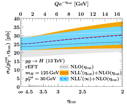
Refer to caption
Refer to caption
Figure -1130: The 0-jet cross section for ggH𝑔𝑔𝐻gg\to H at mH=125GeVsubscript𝑚𝐻125GeVm_{H}=125\,\mathrm{GeV} for pTcut=30GeVsuperscriptsubscript𝑝𝑇cut30GeVp_{T}^{\rm cut}=30\,\mathrm{GeV} (left) and ggX𝑔𝑔𝑋gg\to X at mX=1TeVsubscript𝑚𝑋1TeVm_{X}=1\,\mathrm{TeV} and pTcut=50GeVsuperscriptsubscript𝑝𝑇cut50GeVp_{T}^{\rm cut}=50\,\mathrm{GeV} (right) as a function of ηcutsubscript𝜂cut\eta_{\rm cut}. The same observable (σ0subscript𝜎0\sigma_{0}) is calculated in three different ways, shown by the different bands, as described in the text.

We first consider gluon-fusion Higgs production shown in the left panel of figure -1130, where we set pTcut=30GeVsuperscriptsubscript𝑝𝑇cut30GeVp_{T}^{\rm cut}=30\,\mathrm{GeV}. The NLO(ηcut)subscript𝜂cut(\eta_{\rm cut}) prediction (gray band) exhibits a slight, physical rise in the cross section as ηcutsubscript𝜂cut\eta_{\rm cut} decreases towards the right. This is not surprising as at fixed order, decreasing ηcutsubscript𝜂cut\eta_{\rm cut} simply amounts to accumulating the squared LO1 matrix element over a larger part of phase space. The rise is less pronounced than for the resummed results (orange and blue bands), but still compatible with them within each others’ uncertainties. Comparing NLL(ηcut)+{}^{\prime}(\eta_{\rm cut})+NLO(ηcut)subscript𝜂cut(\eta_{\rm cut}) (orange) to NLL()+{}^{\prime}(\infty)+NLO(ηcut)subscript𝜂cut(\eta_{\rm cut}) (blue) we find that the additional tower of logarithms predicted by NLL(ηcut){}^{\prime}(\eta_{\rm cut}) on top of the fixed NLO ηcutsubscript𝜂cut\eta_{\rm cut} dependence barely affects the central value of the prediction down to ηcut=2subscript𝜂cut2\eta_{\rm cut}=2. This is perhaps not surprising since Qeηcut𝑄superscript𝑒subscript𝜂cutQe^{-\eta_{\rm cut}} is at most half of pTcutsuperscriptsubscript𝑝𝑇cutp_{T}^{\rm cut}, which means we are not far from regime 1. However, we do observe a noticeable increase in the perturbative uncertainty estimate. This is mainly due to the resummation uncertainty, which is reasonable: ΔresumsubscriptΔresum\Delta_{\mathrm{resum}} probes the unknown higher-order finite terms (the RGE boundary condition) and is therefore sensitive to a change of the beam function boundary condition by the ηcutsubscript𝜂cut\eta_{\rm cut} correction ΔIij(1)Δsuperscriptsubscript𝐼𝑖𝑗1\Delta I_{ij}^{(1)} (see section 2.3). On the other hand, ΔIij(1)Δsuperscriptsubscript𝐼𝑖𝑗1\Delta I_{ij}^{(1)} must be large enough to accommodate — up to power corrections — the fixed-order difference to ηcut=subscript𝜂cut\eta_{\rm cut}=\infty (roughly 2pb2pb2\,\mathrm{pb} at ηcut=2.5subscript𝜂cut2.5\eta_{\rm cut}=2.5, as can be read off from the gray line), so we expect an impact on ΔresumsubscriptΔresum\Delta_{\mathrm{resum}} of similar size. Hence, the conclusion is not that the NLL()+{}^{\prime}(\infty)+NLO(ηcut)subscript𝜂cut(\eta_{\rm cut}) result is more precise, but rather that its uncertainty is potentially underestimated because it cannot capture the ηcutsubscript𝜂cut\eta_{\rm cut} dependence.

In the right panel of figure -1130, we show the same results for a hypothetical color-singlet scalar resonance ggX𝑔𝑔𝑋gg\to X at mX=1TeVsubscript𝑚𝑋1TeVm_{X}=1\,\mathrm{TeV} using pTcut=50GeVsuperscriptsubscript𝑝𝑇cut50GeVp_{T}^{\rm cut}=50\,\mathrm{GeV}. [The dimension-five operator mediating the production of X𝑋X is given in eq. (2.33).] The NLO(ηcut)subscript𝜂cut(\eta_{\rm cut}) result (gray) is now off by a large amount already at ηcut=subscript𝜂cut\eta_{\rm cut}=\infty, where it is not covered by the resummed predictions. This is expected because the high production energy of 1TeV1TeV1\,\mathrm{TeV} implies we are deep in the resummation region, even for the larger value of pTcut=50GeVsuperscriptsubscript𝑝𝑇cut50GeVp_{T}^{\rm cut}=50\,\mathrm{GeV}. The central values of the two resummed treatments start to differ below ηcut=3subscript𝜂cut3\eta_{\rm cut}=3 or above Qeηcut50GeVsimilar-to-or-equals𝑄superscript𝑒subscript𝜂cut50GeVQe^{-\eta_{\rm cut}}\simeq 50\,\mathrm{GeV}, where we are now fully in regime 2. However, the main difference is again the larger and likely more reliable uncertainty estimate in the NLL(ηcut){}^{\prime}(\eta_{\rm cut}) prediction.

Refer to caption
Refer to caption
Figure -1129: The 0-jet cross section for Drell-Yan at Q=mZ𝑄subscript𝑚𝑍Q=m_{Z} and pTcut=20GeVsuperscriptsubscript𝑝𝑇cut20GeVp_{T}^{\rm cut}=20\,\mathrm{GeV} (left) and Q=1TeV𝑄1TeVQ=1\,\mathrm{TeV} and pTcut=25GeVsuperscriptsubscript𝑝𝑇cut25GeVp_{T}^{\rm cut}=25\,\mathrm{GeV} (right) as a function of ηcutsubscript𝜂cut\eta_{\rm cut}. The same observable (σ0subscript𝜎0\sigma_{0}) is calculated in three different ways, shown by the different bands, as described in the text. For better readability, all results are normalized to the resummed central value at ηcut=subscript𝜂cut\eta_{\rm cut}=\infty.

In figure -1129 we show the analogous results for Drell-Yan production at Q=mZ𝑄subscript𝑚𝑍Q=m_{Z} using pTcut=20GeVsuperscriptsubscript𝑝𝑇cut20GeVp_{T}^{\rm cut}=20\,\mathrm{GeV} (left panel) and Q=1TeV𝑄1TeVQ=1\,\mathrm{TeV} using pTcut=25GeVsuperscriptsubscript𝑝𝑇cut25GeVp_{T}^{\rm cut}=25\,\mathrm{GeV} (right panel). For better readability, these results are normalized to the resummed 0-jet cross section at ηcut=subscript𝜂cut\eta_{\rm cut}=\infty. While all predictions agree in the slope of the cross section with respect to ηcutsubscript𝜂cut\eta_{\rm cut}, the NLO(ηcut)subscript𝜂cut(\eta_{\rm cut}) result has a constant offset and an unrealistically small uncertainty estimate. At the lower Q100GeVsimilar-to𝑄100GeVQ\sim 100\,\mathrm{GeV}, we find practically no difference between the NLL(ηcut){}^{\prime}(\eta_{\rm cut}) and NLL(){}^{\prime}(\infty) calculations, so here the effects of the jet rapidity cut can safely be included via the fixed-order matching corrections to the regime 1 resummation. At higher production energies, the intrinsic NLL(ηcut){}^{\prime}(\eta_{\rm cut}) ingredients become more relevant, similar to gluon-fusion, as shown by the increasing uncertainty estimates as ηcutsubscript𝜂cut\eta_{\rm cut} decreases. Note that below ηcut=2.5subscript𝜂cut2.5\eta_{\rm cut}=2.5, Qeηcut80GeVgreater-than-or-equivalent-to𝑄superscript𝑒subscript𝜂cut80GeVQe^{-\eta_{\rm cut}}\gtrsim 80\,\mathrm{GeV} becomes large compared to this choice of pTcut=25GeVsuperscriptsubscript𝑝𝑇cut25GeVp_{T}^{\rm cut}=25\,\mathrm{GeV}, so resumming logarithms of pTcut/(Qeηcut)superscriptsubscript𝑝𝑇cut𝑄superscript𝑒subscript𝜂cutp_{T}^{\rm cut}/(Qe^{-\eta_{\rm cut}}) using the regime 3 factorization given in section 2.4 might help reduce the uncertainties.

4.3 Resummed predictions with a sharp rapidity cut

Here, we compare predictions for different values of ηcutsubscript𝜂cut\eta_{\rm cut} as a function of pTcutsuperscriptsubscript𝑝𝑇cutp_{T}^{\rm cut}. Our working order is NLL(ηcut)+{}^{\prime}(\eta_{\rm cut})+NLO(ηcut)subscript𝜂cut(\eta_{\rm cut}) in the notation of the previous section, which from now on we simply refer to as NLL+{}^{\prime}+NLO, i.e., the ηcutsubscript𝜂cut\eta_{\rm cut} dependence is always included in the resummation. We stress that the differences we observe between predictions in this subsection are physical differences due to the different jet rapidity cuts, and not due to different theoretical treatments as in the previous subsection.
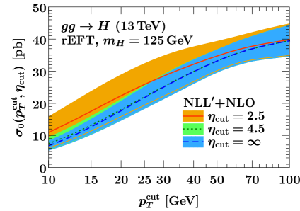
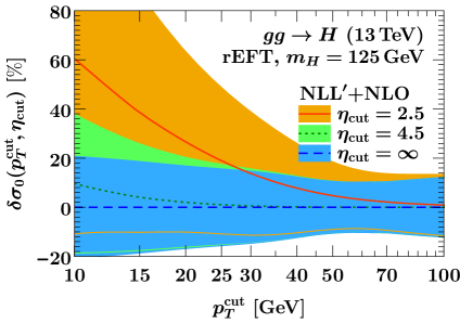
Refer to caption
Refer to caption
Figure -1128: 0-jet cross section σ0(pTcut,ηcut)subscript𝜎0superscriptsubscript𝑝𝑇cutsubscript𝜂cut\sigma_{0}(p_{T}^{\rm cut},\eta_{\rm cut}) for ggH𝑔𝑔𝐻gg\to H for mH=125GeVsubscript𝑚𝐻125GeVm_{H}=125\,\mathrm{GeV} at NLL+NLO for different values of ηcutsubscript𝜂cut\eta_{\rm cut}. The bands indicate the total uncertainty Δμ0ΔφΔresdirect-sumsubscriptΔ𝜇0subscriptΔ𝜑subscriptΔres\Delta_{\mu 0}\oplus\Delta_{\varphi}\oplus\Delta_{\mathrm{res}}. The absolute cross section is shown on the left. On the right, the same results are shown as the percent difference relative to the 0-jet cross section at ηcut=subscript𝜂cut\eta_{\rm cut}=\infty.
σ0(pTcut,ηcut)[pb],ggH(13TeV),rEFT,mH=125GeVformulae-sequencesubscript𝜎0superscriptsubscript𝑝𝑇cutsubscript𝜂cutdelimited-[]pb𝑔𝑔𝐻13TeVrEFTsubscript𝑚𝐻125GeV\sigma_{0}(p_{T}^{\rm cut},\eta_{\rm cut})~{}[\!\,\mathrm{pb}],\,gg\to H\,(13\,\mathrm{TeV}),\,\text{rEFT},\,m_{H}=125\,\mathrm{GeV}
ηcutsubscript𝜂cut\eta_{\rm cut} pTcut=25GeVsuperscriptsubscript𝑝𝑇cut25GeVp_{T}^{\rm cut}=25\,\mathrm{GeV} pTcut=30GeVsuperscriptsubscript𝑝𝑇cut30GeVp_{T}^{\rm cut}=30\,\mathrm{GeV}
2.52.52.5 25.9±3.8μ0±1.5φ±5.0res(25.0%)plus-or-minus25.9subscript3.8𝜇0subscript1.5𝜑subscript5.0respercent25.025.9\!\pm\!3.8_{\mu 0}\!\pm\!1.5_{\varphi}\!\pm\!5.0_{\mathrm{res}}\,(25.0\%) 28.5±4.0μ0±1.6φ±4.6res(22.0%)plus-or-minus28.5subscript4.0𝜇0subscript1.6𝜑subscript4.6respercent22.028.5\!\pm\!4.0_{\mu 0}\!\pm\!1.6_{\varphi}\!\pm\!4.6_{\mathrm{res}}\,(22.0\%)
4.54.54.5 22.0±2.0μ0±1.0φ±2.8res(16.2%)plus-or-minus22.0subscript2.0𝜇0subscript1.0𝜑subscript2.8respercent16.222.0\!\pm\!2.0_{\mu 0}\!\pm\!1.0_{\varphi}\!\pm\!2.8_{\mathrm{res}}\,(16.2\%) 25.2±2.2μ0±1.2φ±2.8res(15.0%)plus-or-minus25.2subscript2.2𝜇0subscript1.2𝜑subscript2.8respercent15.025.2\!\pm\!2.2_{\mu 0}\!\pm\!1.2_{\varphi}\!\pm\!2.8_{\mathrm{res}}\,(15.0\%)
\infty 21.8±1.9μ0±1.0φ±2.7res(15.6%)plus-or-minus21.8subscript1.9𝜇0subscript1.0𝜑subscript2.7respercent15.621.8\!\pm\!1.9_{\mu 0}\!\pm\!1.0_{\varphi}\!\pm\!2.7_{\mathrm{res}}\,(15.6\%) 25.0±2.2μ0±1.2φ±2.7res(14.7%)plus-or-minus25.0subscript2.2𝜇0subscript1.2𝜑subscript2.7respercent14.725.0\!\pm\!2.2_{\mu 0}\!\pm\!1.2_{\varphi}\!\pm\!2.7_{\mathrm{res}}\,(14.7\%)
Table 1: 0-jet cross section for ggH𝑔𝑔𝐻gg\to H for mH=125GeVsubscript𝑚𝐻125GeVm_{H}=125\,\mathrm{GeV} at NLL+NLO for different values of pTcutsuperscriptsubscript𝑝𝑇cutp_{T}^{\rm cut} and ηcutsubscript𝜂cut\eta_{\rm cut} with a breakdown of the uncertainties.

In figure -1128 and table 1 we present results for ggH𝑔𝑔𝐻gg\to H. Going from ηcut=subscript𝜂cut\eta_{\rm cut}=\infty to ηcut=4.5subscript𝜂cut4.5\eta_{\rm cut}=4.5 we find a 1%percent11\% increase of the cross section for the typical values of pTcut=25GeVsuperscriptsubscript𝑝𝑇cut25GeVp_{T}^{\rm cut}=25\,\mathrm{GeV} and 30GeV30GeV30\,\mathrm{GeV}. At ηcut=2.5subscript𝜂cut2.5\eta_{\rm cut}=2.5 the increase becomes more sizable, 14%percent1414\% (19%percent1919\%) for pTcut=30GeVsuperscriptsubscript𝑝𝑇cut30GeVp_{T}^{\rm cut}=30\,\mathrm{GeV} (25GeV25GeV25\,\mathrm{GeV}). The differences vanish as the cross section saturates around pTcut100GeVsimilar-tosuperscriptsubscript𝑝𝑇cut100GeVp_{T}^{\rm cut}\sim 100\,\mathrm{GeV}.

Refer to caption
Refer to caption
Figure -1127: 0-jet cross section σ0(pTcut,ηcut)subscript𝜎0superscriptsubscript𝑝𝑇cutsubscript𝜂cut\sigma_{0}(p_{T}^{\rm cut},\eta_{\rm cut}) for ggX𝑔𝑔𝑋gg\to X for mX=1TeVsubscript𝑚𝑋1TeVm_{X}=1\,\mathrm{TeV} at NLL+NLO for different values of ηcutsubscript𝜂cut\eta_{\rm cut}. The bands indicate the total uncertainty Δμ0ΔφΔresdirect-sumsubscriptΔ𝜇0subscriptΔ𝜑subscriptΔres\Delta_{\mu 0}\oplus\Delta_{\varphi}\oplus\Delta_{\mathrm{res}}. The absolute cross section is shown on the left. On the right, the same results are shown as the percent difference relative to the 0-jet cross section at ηcut=subscript𝜂cut\eta_{\rm cut}=\infty.
σ0(pTcut,ηcut)/|CX|2[pb],ggX(13TeV),Λ=mX=1TeVformulae-sequencesubscript𝜎0superscriptsubscript𝑝𝑇cutsubscript𝜂cutsuperscriptsubscript𝐶𝑋2delimited-[]pb𝑔𝑔𝑋13TeVΛsubscript𝑚𝑋1TeV\sigma_{0}(p_{T}^{\rm cut},\eta_{\rm cut})/\lvert C_{X}\rvert^{2}~{}[\!\,\mathrm{pb}],\,gg\to X\,(13\,\mathrm{TeV}),\,\Lambda=m_{X}=1\,\mathrm{TeV}
ηcutsubscript𝜂cut\eta_{\rm cut} pTcut=50GeVsuperscriptsubscript𝑝𝑇cut50GeVp_{T}^{\rm cut}=50\,\mathrm{GeV} pTcut=100GeVsuperscriptsubscript𝑝𝑇cut100GeVp_{T}^{\rm cut}=100\,\mathrm{GeV}
2.52.52.5 4.9±0.7μ0±0.1φ±1.2res(28.3%)plus-or-minus4.9subscript0.7𝜇0subscript0.1𝜑subscript1.2respercent28.34.9\!\pm\!0.7_{\mu 0}\!\pm\!0.1_{\varphi}\!\pm\!1.2_{\mathrm{res}}\,(28.3\%) 7.8±0.8μ0±0.1φ±1.3res(19.4%)plus-or-minus7.8subscript0.8𝜇0subscript0.1𝜑subscript1.3respercent19.47.8\!\pm\!0.8_{\mu 0}\!\pm\!0.1_{\varphi}\!\pm\!1.3_{\mathrm{res}}\,(19.4\%)
4.54.54.5 4.1±0.3μ0±0.1φ±0.7res(19.6%)plus-or-minus4.1subscript0.3𝜇0subscript0.1𝜑subscript0.7respercent19.64.1\!\pm\!0.3_{\mu 0}\!\pm\!0.1_{\varphi}\!\pm\!0.7_{\mathrm{res}}\,(19.6\%) 7.4±0.6μ0±0.1φ±1.1res(16.4%)plus-or-minus7.4subscript0.6𝜇0subscript0.1𝜑subscript1.1respercent16.47.4\!\pm\!0.6_{\mu 0}\!\pm\!0.1_{\varphi}\!\pm\!1.1_{\mathrm{res}}\,(16.4\%)
\infty 4.1±0.3μ0±0.1φ±0.7res(19.5%)plus-or-minus4.1subscript0.3𝜇0subscript0.1𝜑subscript0.7respercent19.54.1\!\pm\!0.3_{\mu 0}\!\pm\!0.1_{\varphi}\!\pm\!0.7_{\mathrm{res}}\,(19.5\%) 7.4±0.6μ0±0.1φ±1.1res(16.4%)plus-or-minus7.4subscript0.6𝜇0subscript0.1𝜑subscript1.1respercent16.47.4\!\pm\!0.6_{\mu 0}\!\pm\!0.1_{\varphi}\!\pm\!1.1_{\mathrm{res}}\,(16.4\%)
Table 2: 0-jet cross section for ggX𝑔𝑔𝑋gg\to X for mX=1TeVsubscript𝑚𝑋1TeVm_{X}=1\,\mathrm{TeV} at NLL+NLO for different values of pTcutsuperscriptsubscript𝑝𝑇cutp_{T}^{\rm cut} and ηcutsubscript𝜂cut\eta_{\rm cut} with a breakdown of the uncertainties.

The analogous results for ggX𝑔𝑔𝑋gg\to X for mX=1TeVsubscript𝑚𝑋1TeVm_{X}=1\,\mathrm{TeV} are shown in figure -1127 and table 2. At such a high hard scale, the uncertainties for ηcut=2.5subscript𝜂cut2.5\eta_{\rm cut}=2.5 become essentially beyond control for very tight vetoes pTcut25GeVless-than-or-similar-tosuperscriptsubscript𝑝𝑇cut25GeVp_{T}^{\rm cut}\lesssim 25\,\mathrm{GeV}, which would make an additional resummation of lnpTcut/(Qeηcut)superscriptsubscript𝑝𝑇cut𝑄superscript𝑒subscript𝜂cut\ln p_{T}^{\rm cut}/(Qe^{-\eta_{\rm cut}}) as outlined in section 2.4 necessary. As we will see in the next subsection, this effect can be tamed by replacing the sharp rapidity cut by a step in the jet veto. However, for any choice of ηcutsubscript𝜂cut\eta_{\rm cut} the cross section is very strongly Sudakov suppressed for such small values of pTcutsuperscriptsubscript𝑝𝑇cutp_{T}^{\rm cut}. At more realistic values of the veto, the jet rapidity cut for ηcut=2.5subscript𝜂cut2.5\eta_{\rm cut}=2.5 compared to ηcut=subscript𝜂cut\eta_{\rm cut}=\infty still leads to a sizable increase of 20%percent2020\% (5%percent55\%) for pTcut=50GeVsuperscriptsubscript𝑝𝑇cut50GeVp_{T}^{\rm cut}=50\,\mathrm{GeV} (pTcut=100GeVsuperscriptsubscript𝑝𝑇cut100GeVp_{T}^{\rm cut}=100\,\mathrm{GeV}). In contrast, the effect for ηcut=4.5subscript𝜂cut4.5\eta_{\rm cut}=4.5 is very small.

Refer to caption
Refer to caption
Refer to caption
Refer to caption
Figure -1126: The 0-jet cross section dσ0(pTcut,ηcut)/dQdsubscript𝜎0superscriptsubscript𝑝𝑇cutsubscript𝜂cutd𝑄\mathrm{d}\sigma_{0}(p_{T}^{\rm cut},\eta_{\rm cut})/\mathrm{d}Q for Drell-Yan production at the Z𝑍Z pole Q=mZ𝑄subscript𝑚𝑍Q=m_{Z} (top row) and at Q=1TeV𝑄1TeVQ=1\,\mathrm{TeV} (bottom row) at NLL+NLO for different values of ηcutsubscript𝜂cut\eta_{\rm cut}. The bands indicate the total uncertainty Δμ0Δresdirect-sumsubscriptΔ𝜇0subscriptΔres\Delta_{\mu 0}\oplus\Delta_{\mathrm{res}}. The absolute cross section is shown on the left. On the right, the same results are shown as the percent difference relative to the 0-jet cross section at ηcut=subscript𝜂cut\eta_{\rm cut}=\infty.
dσ0(pTcut,ηcut)/dQ[pb/GeV],ppZ/γ+(13TeV),Q=mZformulae-sequencedsubscript𝜎0superscriptsubscript𝑝𝑇cutsubscript𝜂cutd𝑄delimited-[]pbGeV𝑝𝑝𝑍superscript𝛾superscriptsuperscript13TeV𝑄subscript𝑚𝑍\mathrm{d}\sigma_{0}(p_{T}^{\rm cut},\eta_{\rm cut})/\mathrm{d}Q~{}[\!\,\mathrm{pb}/\!\,\mathrm{GeV}],\,pp\to Z/\gamma^{\ast}\to\ell^{+}\ell^{-}\,(13\,\mathrm{TeV}),\,Q=m_{Z}
ηcutsubscript𝜂cut\eta_{\rm cut} pTcut=20GeVsuperscriptsubscript𝑝𝑇cut20GeVp_{T}^{\rm cut}=20\,\mathrm{GeV} pTcut=25GeVsuperscriptsubscript𝑝𝑇cut25GeVp_{T}^{\rm cut}=25\,\mathrm{GeV}
2.52.52.5 362±22μ0±21res(8.5%)plus-or-minus362subscript22𝜇0subscript21respercent8.5362\!\pm\!22_{\mu 0}\!\pm\!21_{\mathrm{res}}\,(8.5\%) 393±22μ0±14res(6.6%)plus-or-minus393subscript22𝜇0subscript14respercent6.6393\!\pm\!22_{\mu 0}\!\pm\!14_{\mathrm{res}}\,(6.6\%)
4.54.54.5 340±24μ0±22res(9.4%)plus-or-minus340subscript24𝜇0subscript22respercent9.4340\!\pm\!24_{\mu 0}\!\pm\!22_{\mathrm{res}}\,(9.4\%) 377±24μ0±15res(7.4%)plus-or-minus377subscript24𝜇0subscript15respercent7.4377\!\pm\!24_{\mu 0}\!\pm\!15_{\mathrm{res}}\,(7.4\%)
\infty 339±24μ0±22res(9.5%)plus-or-minus339subscript24𝜇0subscript22respercent9.5339\!\pm\!24_{\mu 0}\!\pm\!22_{\mathrm{res}}\,(9.5\%) 376±24μ0±15res(7.4%)plus-or-minus376subscript24𝜇0subscript15respercent7.4376\!\pm\!24_{\mu 0}\!\pm\!15_{\mathrm{res}}\,(7.4\%)
dσ0(pTcut,ηcut)/dQ[ab/GeV],ppZ/γ+(13TeV),Q=1TeVformulae-sequencedsubscript𝜎0superscriptsubscript𝑝𝑇cutsubscript𝜂cutd𝑄delimited-[]abGeV𝑝𝑝𝑍superscript𝛾superscriptsuperscript13TeV𝑄1TeV\mathrm{d}\sigma_{0}(p_{T}^{\rm cut},\eta_{\rm cut})/\mathrm{d}Q~{}[\!\,\mathrm{ab}/\!\,\mathrm{GeV}],\,pp\to Z/\gamma^{\ast}\to\ell^{+}\ell^{-}\,(13\,\mathrm{TeV}),\,Q=1\,\mathrm{TeV}
ηcutsubscript𝜂cut\eta_{\rm cut} pTcut=25GeVsuperscriptsubscript𝑝𝑇cut25GeVp_{T}^{\rm cut}=25\,\mathrm{GeV} pTcut=50GeVsuperscriptsubscript𝑝𝑇cut50GeVp_{T}^{\rm cut}=50\,\mathrm{GeV}
2.52.52.5 14.1±0.8μ±1.7res(13.6%)plus-or-minus14.1subscript0.8𝜇subscript1.7respercent13.614.1\!\pm\!0.8_{\mu}\!\pm\!1.7_{\mathrm{res}}\,(13.6\%) 19.7±0.6μ±1.7res(9.0%)plus-or-minus19.7subscript0.6𝜇subscript1.7respercent9.019.7\!\pm\!0.6_{\mu}\!\pm\!1.7_{\mathrm{res}}\,(9.0\%)
4.54.54.5 12.4±0.4μ±1.1res(9.2%)plus-or-minus12.4subscript0.4𝜇subscript1.1respercent9.212.4\!\pm\!0.4_{\mu}\!\pm\!1.1_{\mathrm{res}}\,(9.2\%) 18.9±0.4μ±1.4res(7.6%)plus-or-minus18.9subscript0.4𝜇subscript1.4respercent7.618.9\!\pm\!0.4_{\mu}\!\pm\!1.4_{\mathrm{res}}\,(7.6\%)
\infty 12.4±0.4μ±1.1res(9.1%)plus-or-minus12.4subscript0.4𝜇subscript1.1respercent9.112.4\!\pm\!0.4_{\mu}\!\pm\!1.1_{\mathrm{res}}\,(9.1\%) 18.9±0.4μ±1.4res(7.6%)plus-or-minus18.9subscript0.4𝜇subscript1.4respercent7.618.9\!\pm\!0.4_{\mu}\!\pm\!1.4_{\mathrm{res}}\,(7.6\%)
Table 3: The 0-jet cross section for Drell-Yan production at the Z𝑍Z pole Q=mZ𝑄subscript𝑚𝑍Q=m_{Z} (top) and at Q=1TeV𝑄1TeVQ=1\,\mathrm{TeV} (bottom) at NLL+NLO for different values of pTcutsuperscriptsubscript𝑝𝑇cutp_{T}^{\rm cut} and ηcutsubscript𝜂cut\eta_{\rm cut} with a breakdown of the uncertainties.

The results for Drell-Yan production are given in figure -1126 and table 3. For Q=mZ𝑄subscript𝑚𝑍Q=m_{Z} (top rows), we find a 57%5percent75-7\% increase in the cross section at ηcut=2.5subscript𝜂cut2.5\eta_{\rm cut}=2.5 for pTcut=2025GeVsuperscriptsubscript𝑝𝑇cut2025GeVp_{T}^{\rm cut}=20-25\,\mathrm{GeV}. Here the uncertainty for ηcut=2.5subscript𝜂cut2.5\eta_{\rm cut}=2.5 is under good control even down to pTcut10GeVsimilar-tosuperscriptsubscript𝑝𝑇cut10GeVp_{T}^{\rm cut}\sim 10\,\mathrm{GeV}. For Q=1TeV𝑄1TeVQ=1\,\mathrm{TeV} (bottom rows), the cross section for ηcut=2.5subscript𝜂cut2.5\eta_{\rm cut}=2.5 increases by 14%percent1414\% (4%percent44\%) for pTcut=25GeVsuperscriptsubscript𝑝𝑇cut25GeVp_{T}^{\rm cut}=25\,\mathrm{GeV} (50GeV50GeV50\,\mathrm{GeV}) compared to ηcut=subscript𝜂cut\eta_{\rm cut}=\infty. The Sudakov suppression and the accompanying increase in relative uncertainty at small pTcutsuperscriptsubscript𝑝𝑇cutp_{T}^{\rm cut} are weaker than for ggX𝑔𝑔𝑋gg\to X due to the smaller color factor (CFsubscript𝐶𝐹C_{F} vs. CAsubscript𝐶𝐴C_{A}) in the Sudakov exponent, but are still substantial for a quark-induced process. The effect of the rapidity cut at ηcut=4.5subscript𝜂cut4.5\eta_{\rm cut}=4.5 is negligible.

4.4 Resummed predictions with a step in the jet veto

In the previous subsection we have seen that a sharp rapidity cut at ηcut=2.5subscript𝜂cut2.5\eta_{\rm cut}=2.5 can lead to a substantial loss of precision in the theory predictions, especially for gluon-induced processes and at high production energies.

In figure -1125 we show the resummed 0-jet cross section for ggH𝑔𝑔𝐻gg\to H and ggX𝑔𝑔𝑋gg\to X with a step in the jet veto at ηcut=2.5subscript𝜂cut2.5\eta_{\rm cut}=2.5 as a function of the second jet veto parameter p~Tcutsuperscriptsubscript~𝑝𝑇cut\tilde{p}_{T}^{\rm cut} that is applied beyond ηcutsubscript𝜂cut\eta_{\rm cut}. The central jet veto below ηcutsubscript𝜂cut\eta_{\rm cut} is fixed to pTcut=25GeVsuperscriptsubscript𝑝𝑇cut25GeVp_{T}^{\rm cut}=25\,\mathrm{GeV}. On the left of the plot p~Tcut=pTcutsuperscriptsubscript~𝑝𝑇cutsuperscriptsubscript𝑝𝑇cut\tilde{p}_{T}^{\rm cut}=p_{T}^{\rm cut}, which is equivalent to having no rapidity cut, in which case the uncertainties are well under control. In the limit p~Tcutsuperscriptsubscript~𝑝𝑇cut\tilde{p}_{T}^{\rm cut}\to\infty (towards the right) the step becomes a sharp cut, corresponding to the results of the previous subsection. While the step in the jet veto still leads to an increase in the uncertainties, this can now be controlled by the choice of p~Tcutsuperscriptsubscript~𝑝𝑇cut\tilde{p}_{T}^{\rm cut}. At this order, a small step from pTcut=25GeVsuperscriptsubscript𝑝𝑇cut25GeVp_{T}^{\rm cut}=25\,\mathrm{GeV} to p~Tcut=30GeVsuperscriptsubscript~𝑝𝑇cut30GeV\tilde{p}_{T}^{\rm cut}=30\,\mathrm{GeV} only leads to a small increase in uncertainty. For a larger step to p~Tcut=50GeV=2pTcutsuperscriptsubscript~𝑝𝑇cut50GeV2superscriptsubscript𝑝𝑇cut\tilde{p}_{T}^{\rm cut}=50\,\mathrm{GeV}=2p_{T}^{\rm cut}, the uncertainties already increase substantially but are still much smaller than for a sharp cut.
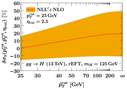
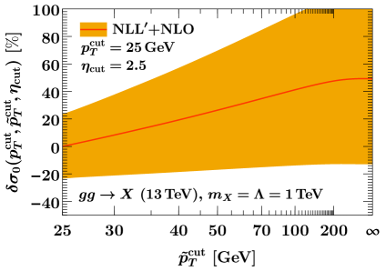
Refer to caption
Refer to caption
Figure -1125: 0-jet cross section σ0(pTcut,p~Tcut,ηcut)subscript𝜎0superscriptsubscript𝑝𝑇cutsuperscriptsubscript~𝑝𝑇cutsubscript𝜂cut\sigma_{0}(p_{T}^{\rm cut},\tilde{p}_{T}^{\rm cut},\eta_{\rm cut}) with a step at ηcut=2.5subscript𝜂cut2.5\eta_{\rm cut}=2.5 for ggH𝑔𝑔𝐻gg\to H (left panel) and ggX𝑔𝑔𝑋gg\to X (right panel) at NLL+NLO. The results are shown for a fixed central veto at pTcut=25GeVsuperscriptsubscript𝑝𝑇cut25GeVp_{T}^{\rm cut}=25\,\mathrm{GeV} as a function of the jet veto p~Tcutsuperscriptsubscript~𝑝𝑇cut\tilde{p}_{T}^{\rm cut} that is applied beyond ηcutsubscript𝜂cut\eta_{\rm cut}. We show the percent differences relative to the result for a uniform veto p~Tcut=pTcutsuperscriptsubscript~𝑝𝑇cutsuperscriptsubscript𝑝𝑇cut\tilde{p}_{T}^{\rm cut}=p_{T}^{\rm cut}. The bands indicate the total uncertainty Δμ0ΔφΔresdirect-sumsubscriptΔ𝜇0subscriptΔ𝜑subscriptΔres\Delta_{\mu 0}\oplus\Delta_{\varphi}\oplus\Delta_{\mathrm{res}}.

5 Conclusion

We have developed a systematic framework to seamlessly incorporate a cut on the rapidity of reconstructed jets, |ηjet|<ηcutsubscript𝜂jetsubscript𝜂cut\lvert\eta_{\rm jet}\rvert<\eta_{\rm cut}, into the theoretical description of jet-vetoed processes at the LHC. We have shown that the standard jet-veto resummation, which neglects the rapidity cut, is correct up to power corrections of 𝒪(Qeηcut/pTcut)𝒪𝑄superscript𝑒subscript𝜂cutsuperscriptsubscript𝑝𝑇cut\mathcal{O}(Qe^{-\eta_{\rm cut}}/p_{T}^{\rm cut}), with Q𝑄Q the hard-interaction scale and pTcutsuperscriptsubscript𝑝𝑇cutp_{T}^{\rm cut} the jet veto cut.

We calculated the necessary ηcutsubscript𝜂cut\eta_{\rm cut}-dependent corrections at one loop as well as all logarithmic contributions to them at two loops (including both small-R𝑅R clustering logarithms and all jet-veto logarithms predicted by the RGE; see section 2.3). The remaining ingredients required for a full NNLL analysis with ηcutsubscript𝜂cut\eta_{\rm cut} effects are finite nonlogarithmic pieces that could be either calculated explicitly or extracted numerically from the full-QCD results, which we leave to future work. In addition, we considered for the first time the case of a step in the jet veto, i.e., an increase in the veto parameter to p~Tcut>pTcutsuperscriptsubscript~𝑝𝑇cutsuperscriptsubscript𝑝𝑇cut\tilde{p}_{T}^{\rm cut}>p_{T}^{\rm cut} beyond ηcutsubscript𝜂cut\eta_{\rm cut}, and showed how to similarly incorporate it into the jet-veto resummation (see section 3.2).

We also considered the jet veto cross section in the limit pTcutQeηcutmuch-less-thansuperscriptsubscript𝑝𝑇cut𝑄superscript𝑒subscript𝜂cutp_{T}^{\rm cut}\ll Qe^{-\eta_{\rm cut}}, corresponding to either very tight vetoes or very central rapidity cuts (see section 2.4). In this regime, the jet-veto resummation becomes impaired by the presence of nonglobal logarithms, requiring a refactorization of the cross section. However, we have argued that this parametric region will most likely not play a role for typical jet binning analyses at the LHC. If experimentally necessary, it can be avoided by replacing the sharp rapidity cut by a moderate step in the jet veto, which is free of nonglobal logarithms (see section 3.4).

There are several important outcomes of our analysis. First, a jet rapidity cut at very forward rapidities due to the finite detector acceptance, ηcut4.5similar-to-or-equalssubscript𝜂cut4.5\eta_{\rm cut}\simeq 4.5, is theoretically safe and unproblematic. In contrast, restricting the jet veto to the more central region, with a sharp rapidity cut at the end of the tracking detectors, ηcut2.5similar-to-or-equalssubscript𝜂cut2.5\eta_{\rm cut}\simeq 2.5, leads to an increase in the perturbative uncertainties (which may not be captured if the jet rapidity cut is not included in the resummation). This loss in theoretical precision can become particularly severe for gluon-induced processes and for processes at high scales. It can however be mitigated by replacing the sharp rapidity cut by a moderate step in the jet veto. We expect this to be a generic feature that also holds at higher orders. It will be interesting to extend our resummed predictions to the next order (NNLL) to confirm this as well as to reduce the overall size of the theoretical uncertainties. We encourage our experimental colleagues to take full advantage of such step-like jet vetoes in order to benefit from suitably tight jet vetoes at central rapidities, while avoiding the increased pile-up contamination in the forward region.

Acknowledgments

We thank Daekyoung Kang, Yiannis Makris, Thomas Mehen, and Iain Stewart for discussions. This work was partially supported by the German Science Foundation (DFG) through the Emmy-Noether Grant No. TA 867/1-1 and the Collaborative Research Center (SFB) 676 Particles, Strings and the Early Universe.

Appendix A Perturbative ingredients

We collect known results for required anomalous dimensions in appendix A.1 and for the standard pTcutsuperscriptsubscript𝑝𝑇cutp_{T}^{\rm cut} beam function without a jet rapidity cut in appendix A.2. In appendix A.3 we provide some details on the computation of the one-loop beam function matching coefficients in eqs. (2.25) and (2.4). In appendix A.4 we compute the soft-collinear functions given in eqs. (2.4) and (3.15). In appendix A.5 we compare to the one-loop results of ref. [34]. In appendix A.6 we discuss the Mellin convolutions required in the two-loop ηcutsubscript𝜂cut\eta_{\rm cut} dependent beam function in eq. (2.3).

A.1 Anomalous dimensions

We expand the β𝛽\beta function of QCD as

μdαs(μ)dμ=β[αs(μ)],β(αs)=2αsn=0βn(αs4π)n+1,formulae-sequence𝜇dsubscript𝛼𝑠𝜇d𝜇𝛽delimited-[]subscript𝛼𝑠𝜇𝛽subscript𝛼𝑠2subscript𝛼𝑠superscriptsubscript𝑛0subscript𝛽𝑛superscriptsubscript𝛼𝑠4𝜋𝑛1\mu\frac{\mathrm{d}\alpha_{s}(\mu)}{\mathrm{d}\mu}=\beta[\alpha_{s}(\mu)]\,,\qquad\beta(\alpha_{s})=-2\alpha_{s}\sum_{n=0}^{\infty}\beta_{n}\left(\frac{\alpha_{s}}{4\pi}\right)^{n+1}\,, (A.1)

with the one-loop and two-loop coefficients in the MS¯¯MS\overline{\text{MS}} scheme given by

β0=113CA43TFnf,β1=343CA2(203CA+4CF)TFnf.formulae-sequencesubscript𝛽0113subscript𝐶𝐴43subscript𝑇𝐹subscript𝑛𝑓subscript𝛽1343superscriptsubscript𝐶𝐴2203subscript𝐶𝐴4subscript𝐶𝐹subscript𝑇𝐹subscript𝑛𝑓\displaystyle\beta_{0}=\frac{11}{3}\,C_{A}-\frac{4}{3}\,T_{F}\,n_{f}\,,\qquad\beta_{1}=\frac{34}{3}\,C_{A}^{2}-\Bigl{(}\frac{20}{3}\,C_{A}\,+4C_{F}\Bigr{)}\,T_{F}\,n_{f}\,. (A.2)

The cusp and all noncusp anomalous dimensions γ(αs)𝛾subscript𝛼𝑠\gamma(\alpha_{s}) are expanded as

Γcuspi(αs)=n=0Γni(αs4π)n+1,γ(αs)=n=0γn(αs4π)n+1.formulae-sequencesubscriptsuperscriptΓ𝑖cuspsubscript𝛼𝑠superscriptsubscript𝑛0subscriptsuperscriptΓ𝑖𝑛superscriptsubscript𝛼𝑠4𝜋𝑛1𝛾subscript𝛼𝑠superscriptsubscript𝑛0subscript𝛾𝑛superscriptsubscript𝛼𝑠4𝜋𝑛1\Gamma^{i}_{\mathrm{cusp}}(\alpha_{s})=\sum_{n=0}^{\infty}\Gamma^{i}_{n}\Bigl{(}\frac{\alpha_{s}}{4\pi}\Bigr{)}^{n+1}\,,\qquad\gamma(\alpha_{s})=\sum_{n=0}^{\infty}\gamma_{n}\Bigl{(}\frac{\alpha_{s}}{4\pi}\Bigr{)}^{n+1}\,. (A.3)

The coefficients of the MS¯¯MS\overline{\text{MS}} cusp anomalous dimension through two loops are

ΓnqsubscriptsuperscriptΓ𝑞𝑛\displaystyle\Gamma^{q}_{n} =CFΓn,Γng=CAΓn,(for n=0,1,2),formulae-sequenceabsentsubscript𝐶𝐹subscriptΓ𝑛subscriptsuperscriptΓ𝑔𝑛subscript𝐶𝐴subscriptΓ𝑛(for n=0,1,2)\displaystyle=C_{F}\Gamma_{n}\,,\qquad\Gamma^{g}_{n}=C_{A}\Gamma_{n}\,,\qquad\text{(for $n=0,1,2$)}\,,
Γ0subscriptΓ0\displaystyle\Gamma_{0} =4,absent4\displaystyle=4\,,
Γ1subscriptΓ1\displaystyle\Gamma_{1} =4[CA(679π23)209TFnf]=43[(4π2)CA+5β0].absent4delimited-[]subscript𝐶𝐴679superscript𝜋23209subscript𝑇𝐹subscript𝑛𝑓43delimited-[]4superscript𝜋2subscript𝐶𝐴5subscript𝛽0\displaystyle=4\Bigl{[}C_{A}\Bigl{(}\frac{67}{9}-\frac{\pi^{2}}{3}\Bigr{)}-\frac{20}{9}\,T_{F}\,n_{f}\Bigr{]}=\frac{4}{3}\bigl{[}(4-\pi^{2})C_{A}+5\beta_{0}\bigr{]}\,. (A.4)

The PDF anomalous dimension in eq. (2.23) is expanded as

Pij(αs,z)=n=0Pij(n)(z)(αs4π)n+1.subscript𝑃𝑖𝑗subscript𝛼𝑠𝑧superscriptsubscript𝑛0subscriptsuperscript𝑃𝑛𝑖𝑗𝑧superscriptsubscript𝛼𝑠4𝜋𝑛1P_{ij}(\alpha_{s},z)=\sum_{n=0}^{\infty}P^{(n)}_{ij}(z)\left(\frac{\alpha_{s}}{4\pi}\right)^{n+1}\,. (A.5)

Note that we expand the PDF anomalous dimension in αs/(4π)subscript𝛼𝑠4𝜋\alpha_{s}/(4\pi) and not αs/(2π)subscript𝛼𝑠2𝜋\alpha_{s}/(2\pi) as is often done. The one-loop coefficients of the PDF anomalous dimension read

Pqiqj(0)(z)subscriptsuperscript𝑃0subscript𝑞𝑖subscript𝑞𝑗𝑧\displaystyle P^{(0)}_{q_{i}q_{j}}(z) =Pq¯iq¯j(0)(z)=2CFδijθ(z)Pqq(z),absentsubscriptsuperscript𝑃0subscript¯𝑞𝑖subscript¯𝑞𝑗𝑧2subscript𝐶𝐹subscript𝛿𝑖𝑗𝜃𝑧subscript𝑃𝑞𝑞𝑧\displaystyle=P^{(0)}_{\bar{q}_{i}\bar{q}_{j}}(z)=2C_{F}\,\delta_{ij}\,\theta(z)P_{qq}(z)\,,\quad Pgg(0)(z)subscriptsuperscript𝑃0𝑔𝑔𝑧\displaystyle P^{(0)}_{gg}(z) =2CAθ(z)Pgg(z)+β0δ(1z),absent2subscript𝐶𝐴𝜃𝑧subscript𝑃𝑔𝑔𝑧subscript𝛽0𝛿1𝑧\displaystyle=2C_{A}\,\theta(z)P_{gg}(z)+\beta_{0}\,\delta(1-z)\,,
Pqig(0)(z)subscriptsuperscript𝑃0subscript𝑞𝑖𝑔𝑧\displaystyle P^{(0)}_{q_{i}g}(z) =Pq¯ig(0)(z)=2TFθ(z)Pqg(z),absentsubscriptsuperscript𝑃0subscript¯𝑞𝑖𝑔𝑧2subscript𝑇𝐹𝜃𝑧subscript𝑃𝑞𝑔𝑧\displaystyle=P^{(0)}_{\bar{q}_{i}g}(z)=2T_{F}\,\theta(z)P_{qg}(z)\,,\quad Pgqi(0)(z)subscriptsuperscript𝑃0𝑔subscript𝑞𝑖𝑧\displaystyle P^{(0)}_{gq_{i}}(z) =Pgq¯i(0)(z)=2CFθ(z)Pgq(z),absentsubscriptsuperscript𝑃0𝑔subscript¯𝑞𝑖𝑧2subscript𝐶𝐹𝜃𝑧subscript𝑃𝑔𝑞𝑧\displaystyle=P^{(0)}_{g\bar{q}_{i}}(z)=2C_{F}\,\theta(z)P_{gq}(z)\,, (A.6)

in terms of the standard color-stripped one-loop QCD splitting functions

Pqq(z)subscript𝑃𝑞𝑞𝑧\displaystyle P_{qq}(z) =20(1z)θ(1z)(1+z)+32δ(1z)absent2subscript01𝑧𝜃1𝑧1𝑧32𝛿1𝑧\displaystyle=2\mathcal{L}_{0}(1-z)-\theta(1-z)(1+z)+\frac{3}{2}\delta(1-z) =[θ(1z)1+z21z]+,absentsubscriptdelimited-[]𝜃1𝑧1superscript𝑧21𝑧\displaystyle=\Bigl{[}\theta(1-z)\frac{1+z^{2}}{1-z}\Bigr{]}_{+}\,,
Pgg(z)subscript𝑃𝑔𝑔𝑧\displaystyle P_{gg}(z) =20(1z)+θ(1z)[2z(1z)+2(1z)z2]absent2subscript01𝑧𝜃1𝑧delimited-[]2𝑧1𝑧21𝑧𝑧2\displaystyle=2\mathcal{L}_{0}(1-z)+\theta(1-z)\Bigl{[}2z(1-z)+\frac{2(1-z)}{z}-2\Bigr{]}\, = 20(1z)(1z+z2)2z,absent2subscript01𝑧superscript1𝑧superscript𝑧22𝑧\displaystyle=\,2\mathcal{L}_{0}(1-z)\frac{(1-z+z^{2})^{2}}{z}\,,
Pqg(z)subscript𝑃𝑞𝑔𝑧\displaystyle P_{qg}(z) =θ(1z)[12z(1z)],absent𝜃1𝑧delimited-[]12𝑧1𝑧\displaystyle=\theta(1-z)\bigl{[}1-2z(1-z)\bigr{]}\,,
Pgq(z)subscript𝑃𝑔𝑞𝑧\displaystyle P_{gq}(z) =θ(1z)1+(1z)2z.absent𝜃1𝑧1superscript1𝑧2𝑧\displaystyle=\theta(1-z)\frac{1+(1-z)^{2}}{z}\,. (A.7)

The two-loop coefficients were calculated in refs. [67, 68, 69]. They can be decomposed as

Pqiqj(1)(z)=Pq¯iq¯j(1)(z)subscriptsuperscript𝑃1subscript𝑞𝑖subscript𝑞𝑗𝑧subscriptsuperscript𝑃1subscript¯𝑞𝑖subscript¯𝑞𝑗𝑧\displaystyle P^{(1)}_{q_{i}q_{j}}(z)=P^{(1)}_{\bar{q}_{i}\bar{q}_{j}}(z) =4CFθ(z)[δijPqqV1(z)+PqqS1(z)],absent4subscript𝐶𝐹𝜃𝑧delimited-[]subscript𝛿𝑖𝑗subscriptsuperscript𝑃1𝑞𝑞𝑉𝑧subscriptsuperscript𝑃1𝑞𝑞𝑆𝑧\displaystyle=4C_{F}\,\theta(z)\bigl{[}\delta_{ij}P^{1}_{qqV}(z)+P^{1}_{qqS}(z)\bigr{]}\,,
Pqig(1)(z)=Pq¯ig(1)(z)subscriptsuperscript𝑃1subscript𝑞𝑖𝑔𝑧subscriptsuperscript𝑃1subscript¯𝑞𝑖𝑔𝑧\displaystyle P^{(1)}_{q_{i}g}(z)=P^{(1)}_{\bar{q}_{i}g}(z) =4TFθ(z)Pqg1,absent4subscript𝑇𝐹𝜃𝑧subscriptsuperscript𝑃1𝑞𝑔\displaystyle=4T_{F}\,\theta(z)\,P^{1}_{qg}\,,
Pqiq¯j(1)(z)=Pq¯iqj(1)(z)subscriptsuperscript𝑃1subscript𝑞𝑖subscript¯𝑞𝑗𝑧subscriptsuperscript𝑃1subscript¯𝑞𝑖subscript𝑞𝑗𝑧\displaystyle P^{(1)}_{q_{i}\bar{q}_{j}}(z)=P^{(1)}_{\bar{q}_{i}q_{j}}(z) =4CFθ(z)[δijPqq¯V1(z)+PqqS1(z)],absent4subscript𝐶𝐹𝜃𝑧delimited-[]subscript𝛿𝑖𝑗subscriptsuperscript𝑃1𝑞¯𝑞𝑉𝑧subscriptsuperscript𝑃1𝑞𝑞𝑆𝑧\displaystyle=4C_{F}\,\theta(z)\bigl{[}\delta_{ij}P^{1}_{q\bar{q}V}(z)+P^{1}_{qqS}(z)\bigr{]}\,,
Pgg(1)(z)subscriptsuperscript𝑃1𝑔𝑔𝑧\displaystyle P^{(1)}_{gg}(z) =4θ(z)[CAPggA1+TFnfPggF1],absent4𝜃𝑧delimited-[]subscript𝐶𝐴subscriptsuperscript𝑃1𝑔𝑔𝐴subscript𝑇𝐹subscript𝑛𝑓subscriptsuperscript𝑃1𝑔𝑔𝐹\displaystyle=4\theta(z)\bigl{[}C_{A}P^{1}_{ggA}+T_{F}n_{f}\,P^{1}_{ggF}\bigr{]}\,,
Pgqi(1)(z)=Pgq¯i(1)(z)subscriptsuperscript𝑃1𝑔subscript𝑞𝑖𝑧subscriptsuperscript𝑃1𝑔subscript¯𝑞𝑖𝑧\displaystyle P^{(1)}_{gq_{i}}(z)=P^{(1)}_{g\bar{q}_{i}}(z) =4CFθ(z)Pgq1,absent4subscript𝐶𝐹𝜃𝑧subscriptsuperscript𝑃1𝑔𝑞\displaystyle=4C_{F}\theta(z)\,P^{1}_{gq}\,, (A.8)

where explicit expressions for the P1superscript𝑃1P^{1} functions on the right-hand side can be found in appendices A of refs. [70, 71]. [Note that in refs. [70, 71] the superscript “111” here is written as “(1)1(1)” there, and the PDF anomalous dimension is expanded there in αs/(2π)subscript𝛼𝑠2𝜋\alpha_{s}/(2\pi), which is already accounted for by the overall factors of 4 on the right-hand side of eq. (A.1).] Explicit results for the Mellin convolutions of two color-stripped leading-order splitting functions can also be found there.

The coefficients of the noncusp beam anomalous dimension are [13, 24]

γB 0qsubscriptsuperscript𝛾𝑞𝐵 0\displaystyle\gamma^{q}_{B\,0} =6CF,absent6subscript𝐶𝐹\displaystyle=6C_{F}\,,
γB 1qsubscriptsuperscript𝛾𝑞𝐵1\displaystyle\gamma^{q}_{B\,1} =CF[(34π2+48ζ3)CF+(14+16(1+π2)ln296ζ3)CA\displaystyle=C_{F}\Bigl{[}(3-4\pi^{2}+48\zeta_{3})C_{F}+\bigl{(}-14+16(1+\pi^{2})\ln 2-96\zeta_{3}\bigr{)}C_{A}
+(19343π2+803ln2)β0],\displaystyle\phantom{=C_{F}a}+\Bigl{(}\frac{19}{3}-\frac{4}{3}\pi^{2}+\frac{80}{3}\ln 2\Bigr{)}\beta_{0}\Bigr{]}\,,
γB 0gsuperscriptsubscript𝛾𝐵 0𝑔\displaystyle\gamma_{B\,0}^{g} =2β0,absent2subscript𝛽0\displaystyle=2\beta_{0}\,,
γB 1gsuperscriptsubscript𝛾𝐵1𝑔\displaystyle\gamma_{B\,1}^{g} =2β1+8CA[(54+2(1+π2)ln26ζ3)CA+(524π23+103ln2)β0]absent2subscript𝛽18subscript𝐶𝐴delimited-[]5421superscript𝜋226subscript𝜁3subscript𝐶𝐴524superscript𝜋231032subscript𝛽0\displaystyle=2\beta_{1}+8C_{A}\biggl{[}\Bigl{(}-\frac{5}{4}+2(1+\pi^{2})\ln 2-6\zeta_{3}\Bigr{)}C_{A}+\Bigl{(}\frac{5}{24}-\frac{\pi^{2}}{3}+\frac{10}{3}\ln 2\Bigr{)}\beta_{0}\biggr{]} (A.9)

The coefficients of the rapidity noncusp anomalous dimension depend on the jet radius R𝑅R. They read [13]

γν 0i(R)superscriptsubscript𝛾𝜈 0𝑖𝑅\displaystyle\gamma_{\nu\,0}^{i}(R) =0,absent0\displaystyle=0\,, (A.10)
γν 1i(R)superscriptsubscript𝛾𝜈1𝑖𝑅\displaystyle\gamma_{\nu\,1}^{i}(R) =16Ci[(179(1+π2)ln2+ζ3)CA+(49+π21253ln2)β0]+C2i(R).\displaystyle=-16C_{i}\biggl{[}\Bigl{(}\frac{17}{9}-(1+\pi^{2})\ln 2+\zeta_{3}\Bigl{)}C_{A}+\Bigl{(}\frac{4}{9}+\frac{\pi^{2}}{12}-\frac{5}{3}\ln 2\Bigl{)}\beta_{0}\biggr{]}+C_{2}^{i}(R)\,.

Here Ci=CF(CA)subscript𝐶𝑖subscript𝐶𝐹subscript𝐶𝐴C_{i}=C_{F}\,(C_{A}) for i=q(g)𝑖𝑞𝑔i=q\,(g) and C2i(R)superscriptsubscript𝐶2𝑖𝑅C_{2}^{i}(R) is the clustering correction due to the jet algorithm relative to a global ETsubscript𝐸𝑇E_{T} veto, as computed in refs. [8, 13],

C2i(R)superscriptsubscript𝐶2𝑖𝑅\displaystyle C_{2}^{i}(R) =16CiciiRlnR+15.62CiCA9.17Ciβ0+𝒪(R2).absent16subscript𝐶𝑖subscriptsuperscript𝑐𝑅𝑖𝑖𝑅15.62subscript𝐶𝑖subscript𝐶𝐴9.17subscript𝐶𝑖subscript𝛽0𝒪superscript𝑅2\displaystyle=16C_{i}c^{R}_{ii}\ln R+15.62\,C_{i}C_{A}-9.17\,C_{i}\beta_{0}+\mathcal{O}(R^{2})\,. (A.11)

The small-R𝑅R clustering coefficient cii=cgg=cqqsubscript𝑐𝑖𝑖subscript𝑐𝑔𝑔subscript𝑐𝑞𝑞c_{ii}=c_{gg}=c_{qq} is given in eq. (2.3).

A.2 Beam function master formula for 𝜼𝐜𝐮𝐭bold-→subscript𝜼𝐜𝐮𝐭\eta_{\rm cut}\to\infty

In analogy to eq. (2.3) the matching coefficient ij(pTcut,R,ω,z,μ,ν)subscript𝑖𝑗superscriptsubscript𝑝𝑇cut𝑅𝜔𝑧𝜇𝜈{\mathcal{I}}_{ij}(p_{T}^{\rm cut},R,\omega,z,\mu,\nu) of the ηcutsubscript𝜂cut\eta_{\rm cut}\to\infty beam functions satisfies (suppressing all other arguments of ijsubscript𝑖𝑗{\mathcal{I}}_{ij})

μddμij(z)𝜇dd𝜇subscript𝑖𝑗𝑧\displaystyle\mu\frac{\mathrm{d}}{\mathrm{d}\mu}{\mathcal{I}}_{ij}(z) =γBi(ω,μ,ν)ij(z)kik(z)z2Pkj[αs(μ),z],absentsubscriptsuperscript𝛾𝑖𝐵𝜔𝜇𝜈subscript𝑖𝑗𝑧subscript𝑘subscripttensor-product𝑧subscript𝑖𝑘𝑧2subscript𝑃𝑘𝑗subscript𝛼𝑠𝜇𝑧\displaystyle=\gamma^{i}_{B}(\omega,\mu,\nu)\,{\mathcal{I}}_{ij}(z)-\sum_{k}{\mathcal{I}}_{ik}(z)\otimes_{z}2P_{kj}[\alpha_{s}(\mu),z]\,,
νddνij(z)𝜈dd𝜈subscript𝑖𝑗𝑧\displaystyle\nu\frac{\mathrm{d}}{\mathrm{d}\nu}{\mathcal{I}}_{ij}(z) =γν,Bi(pTcut,R,μ)ij(z).absentsubscriptsuperscript𝛾𝑖𝜈𝐵superscriptsubscript𝑝𝑇cut𝑅𝜇subscript𝑖𝑗𝑧\displaystyle=\gamma^{i}_{\nu,B}(p_{T}^{\rm cut},R,\mu)\,{\mathcal{I}}_{ij}(z)\,. (A.12)

Solving this order by order in αssubscript𝛼𝑠\alpha_{s} yields the beam function master formula,

ij(z)subscript𝑖𝑗𝑧\displaystyle{\mathcal{I}}_{ij}(z) =δijδ(1z)+αs(μ)4πij(1)(z)+αs2(μ)(4π)2ij(2)(z)+𝒪(αs3),absentsubscript𝛿𝑖𝑗𝛿1𝑧subscript𝛼𝑠𝜇4𝜋superscriptsubscript𝑖𝑗1𝑧superscriptsubscript𝛼𝑠2𝜇superscript4𝜋2superscriptsubscript𝑖𝑗2𝑧𝒪superscriptsubscript𝛼𝑠3\displaystyle=\delta_{ij}\delta(1-z)+\frac{\alpha_{s}(\mu)}{4\pi}\,{\mathcal{I}}_{ij}^{(1)}(z)+\frac{\alpha_{s}^{2}(\mu)}{(4\pi)^{2}}\,{\mathcal{I}}_{ij}^{(2)}(z)+\mathcal{O}(\alpha_{s}^{3})\,,
ij(1)(z)superscriptsubscript𝑖𝑗1𝑧\displaystyle{\mathcal{I}}_{ij}^{(1)}(z) =δijδ(1z)LBμ(2Γ0iLBν+γB 0i)2LBμPij(0)(z)+Iij(1)(z),absentsubscript𝛿𝑖𝑗𝛿1𝑧subscriptsuperscript𝐿𝜇𝐵2subscriptsuperscriptΓ𝑖0subscriptsuperscript𝐿𝜈𝐵subscriptsuperscript𝛾𝑖𝐵 02subscriptsuperscript𝐿𝜇𝐵superscriptsubscript𝑃𝑖𝑗0𝑧superscriptsubscript𝐼𝑖𝑗1𝑧\displaystyle=\delta_{ij}\delta(1-z)\,L^{\mu}_{B}(2\Gamma^{i}_{0}L^{\nu}_{B}+\gamma^{i}_{B\,0})-2L^{\mu}_{B}P_{ij}^{(0)}(z)+I_{ij}^{(1)}(z)\,,
ij(2)(z)superscriptsubscript𝑖𝑗2𝑧\displaystyle{\mathcal{I}}_{ij}^{(2)}(z) =δijδ(1z){(LBμ)2[2(Γ0i)2(LBν)2+LBν(2β0Γ0i+2Γ0iγB 0i)+β0γB 0i+(γB 0i)22]\displaystyle=\delta_{ij}\delta(1-z)\biggl{\{}(L^{\mu}_{B})^{2}\Bigl{[}2(\Gamma^{i}_{0})^{2}(L^{\nu}_{B})^{2}+L^{\nu}_{B}(2\beta_{0}\Gamma^{i}_{0}+2\Gamma^{i}_{0}\gamma^{i}_{B\,0})+\beta_{0}\gamma^{i}_{B\,0}+\frac{(\gamma^{i}_{B\,0})^{2}}{2}\Bigr{]}
+LBμ[2Γ1iLBν+γB 1i]12γν 1i(R)LBν}\displaystyle\quad\quad\quad\quad\quad\quad+L^{\mu}_{B}\Bigl{[}2\Gamma^{i}_{1}L^{\nu}_{B}+\gamma^{i}_{B\,1}\Bigr{]}-\frac{1}{2}\gamma^{i}_{\nu\,1}(R)L^{\nu}_{B}\biggr{\}}
+Pij(0)(z)(LBμ)2[4Γ0iLBν2β02γB 0i]+Iij(1)(z)LBμ[2Γ0iLBν+2β0+γB 0i]superscriptsubscript𝑃𝑖𝑗0𝑧superscriptsubscriptsuperscript𝐿𝜇𝐵2delimited-[]4subscriptsuperscriptΓ𝑖0subscriptsuperscript𝐿𝜈𝐵2subscript𝛽02subscriptsuperscript𝛾𝑖𝐵 0superscriptsubscript𝐼𝑖𝑗1𝑧subscriptsuperscript𝐿𝜇𝐵delimited-[]2subscriptsuperscriptΓ𝑖0subscriptsuperscript𝐿𝜈𝐵2subscript𝛽0subscriptsuperscript𝛾𝑖𝐵 0\displaystyle\quad+P_{ij}^{(0)}(z)\,(L^{\mu}_{B})^{2}\Bigl{[}-4\Gamma^{i}_{0}L^{\nu}_{B}-2\beta_{0}-2\gamma^{i}_{B\,0}\Bigr{]}+I_{ij}^{(1)}(z)\,L^{\mu}_{B}\Bigl{[}2\Gamma^{i}_{0}L^{\nu}_{B}+2\beta_{0}+\gamma^{i}_{B\,0}\Bigr{]}
2LBμkIik(1)(z)zPkj(0)(z)2LBμPij(1)(z)+2(LBμ)2kPik(0)(z)zPkj(0)(z)2subscriptsuperscript𝐿𝜇𝐵subscript𝑘subscripttensor-product𝑧superscriptsubscript𝐼𝑖𝑘1𝑧superscriptsubscript𝑃𝑘𝑗0𝑧2subscriptsuperscript𝐿𝜇𝐵superscriptsubscript𝑃𝑖𝑗1𝑧2superscriptsubscriptsuperscript𝐿𝜇𝐵2subscript𝑘subscripttensor-product𝑧superscriptsubscript𝑃𝑖𝑘0𝑧superscriptsubscript𝑃𝑘𝑗0𝑧\displaystyle\quad-2L^{\mu}_{B}\sum_{k}I_{ik}^{(1)}(z)\otimes_{z}P_{kj}^{(0)}(z)-2L^{\mu}_{B}P_{ij}^{(1)}(z)+2(L^{\mu}_{B})^{2}\sum_{k}P_{ik}^{(0)}(z)\otimes_{z}P_{kj}^{(0)}(z)
+Iij(2)(R,z).superscriptsubscript𝐼𝑖𝑗2𝑅𝑧\displaystyle\quad+I_{ij}^{(2)}(R,z)\,. (A.13)

where we abbreviated

LBμ=lnμpTcut,LBν=lnνω.formulae-sequencesuperscriptsubscript𝐿𝐵𝜇𝜇superscriptsubscript𝑝𝑇cutsuperscriptsubscript𝐿𝐵𝜈𝜈𝜔L_{B}^{\mu}=\ln\frac{\mu}{p_{T}^{\rm cut}}\,,\quad L_{B}^{\nu}=\ln\frac{\nu}{\omega}\,. (A.14)

The one-loop finite terms Iij(1)superscriptsubscript𝐼𝑖𝑗1I_{ij}^{(1)} using the η𝜂\eta regulator [58, 59] are given by (see e.g. refs. [13, 19, 24])

Iqiqj(1)(z)=Iq¯iq¯j(1)(z)subscriptsuperscript𝐼1subscript𝑞𝑖subscript𝑞𝑗𝑧subscriptsuperscript𝐼1subscript¯𝑞𝑖subscript¯𝑞𝑗𝑧\displaystyle I^{(1)}_{q_{i}q_{j}}(z)=I^{(1)}_{\bar{q}_{i}\bar{q}_{j}}(z) =CFδijθ(z)θ(1z) 2(1z),absentsubscript𝐶𝐹subscript𝛿𝑖𝑗𝜃𝑧𝜃1𝑧21𝑧\displaystyle=C_{F}\,\delta_{ij}\,\theta(z)\theta(1-z)\,2(1-z)\,,
Iqig(1)(z)=Iq¯ig(1)(z)subscriptsuperscript𝐼1subscript𝑞𝑖𝑔𝑧subscriptsuperscript𝐼1subscript¯𝑞𝑖𝑔𝑧\displaystyle I^{(1)}_{q_{i}g}(z)=I^{(1)}_{\bar{q}_{i}g}(z) =TFθ(z)θ(1z) 4z(1z),absentsubscript𝑇𝐹𝜃𝑧𝜃1𝑧4𝑧1𝑧\displaystyle=T_{F}\,\theta(z)\theta(1-z)\,4z(1-z)\,,
Igg(1)(z)subscriptsuperscript𝐼1𝑔𝑔𝑧\displaystyle I^{(1)}_{gg}(z) =0,absent0\displaystyle=0\,,
Igqi(1)(z)=Igq¯i(1)(z)subscriptsuperscript𝐼1𝑔subscript𝑞𝑖𝑧subscriptsuperscript𝐼1𝑔subscript¯𝑞𝑖𝑧\displaystyle I^{(1)}_{gq_{i}}(z)=I^{(1)}_{g\bar{q}_{i}}(z) =CFθ(z)θ(1z) 2z.absentsubscript𝐶𝐹𝜃𝑧𝜃1𝑧2𝑧\displaystyle=C_{F}\,\theta(z)\theta(1-z)\,2z\,. (A.15)

Their convolutions with leading-order splitting functions always appear in the form

[I(1)P(0)]ij(z)subscriptdelimited-[]tensor-productsuperscript𝐼1superscript𝑃0𝑖𝑗𝑧\displaystyle\bigl{[}I^{(1)}\otimes P^{(0)}\bigr{]}_{ij}(z) kIik(1)(z)zPkj(0)(z).absentsubscript𝑘subscripttensor-product𝑧superscriptsubscript𝐼𝑖𝑘1𝑧superscriptsubscript𝑃𝑘𝑗0𝑧\displaystyle\equiv\sum_{k}I_{ik}^{(1)}(z)\otimes_{z}P_{kj}^{(0)}(z)\,. (A.16)

For quark-to-(anti)quark transitions we decompose the above flavor structure as

[I(1)P(0)]qiqjsubscriptdelimited-[]tensor-productsuperscript𝐼1superscript𝑃0subscript𝑞𝑖subscript𝑞𝑗\displaystyle\bigl{[}I^{(1)}\otimes P^{(0)}\bigr{]}_{q_{i}q_{j}} =[I(1)P(0)]q¯iq¯jabsentsubscriptdelimited-[]tensor-productsuperscript𝐼1superscript𝑃0subscript¯𝑞𝑖subscript¯𝑞𝑗\displaystyle=\bigl{[}I^{(1)}\otimes P^{(0)}\bigr{]}_{\bar{q}_{i}\bar{q}_{j}} δij[I(1)P(0)]qqV+[I(1)P(0)]qqS,absentsubscript𝛿𝑖𝑗subscriptdelimited-[]tensor-productsuperscript𝐼1superscript𝑃0𝑞𝑞𝑉subscriptdelimited-[]tensor-productsuperscript𝐼1superscript𝑃0𝑞𝑞𝑆\displaystyle\equiv\delta_{ij}\,\bigl{[}I^{(1)}\otimes P^{(0)}\bigr{]}_{qqV}+\bigl{[}I^{(1)}\otimes P^{(0)}\bigr{]}_{qqS}\,,
[I(1)P(0)]qiq¯jsubscriptdelimited-[]tensor-productsuperscript𝐼1superscript𝑃0subscript𝑞𝑖subscript¯𝑞𝑗\displaystyle\bigl{[}I^{(1)}\otimes P^{(0)}\bigr{]}_{q_{i}\bar{q}_{j}} =[I(1)P(0)]qiq¯jabsentsubscriptdelimited-[]tensor-productsuperscript𝐼1superscript𝑃0subscript𝑞𝑖subscript¯𝑞𝑗\displaystyle=\bigl{[}I^{(1)}\otimes P^{(0)}\bigr{]}_{q_{i}\bar{q}_{j}} =[I(1)P(0)]qqS.absentsubscriptdelimited-[]tensor-productsuperscript𝐼1superscript𝑃0𝑞𝑞𝑆\displaystyle=\bigl{[}I^{(1)}\otimes P^{(0)}\bigr{]}_{qqS}\,. (A.17)

The building blocks on the right, together with the gluon-to-quark case, are given by

[I(1)P(0)]qqVsubscriptdelimited-[]tensor-productsuperscript𝐼1superscript𝑃0𝑞𝑞𝑉\displaystyle\bigl{[}I^{(1)}\otimes P^{(0)}\bigr{]}_{qqV} =4CF2θ(z)θ(1z)(1z)[2ln(1z)lnz12],absent4superscriptsubscript𝐶𝐹2𝜃𝑧𝜃1𝑧1𝑧delimited-[]21𝑧𝑧12\displaystyle=4C_{F}^{2}\,\theta(z)\theta(1-z)\,(1-z)\Bigl{[}2\ln(1-z)-\ln z-\frac{1}{2}\Bigr{]}\,,
[I(1)P(0)]qqSsubscriptdelimited-[]tensor-productsuperscript𝐼1superscript𝑃0𝑞𝑞𝑆\displaystyle\bigl{[}I^{(1)}\otimes P^{(0)}\bigr{]}_{qqS} =4TFCFθ(z)θ(1z)(43z2+23z2zlnz2),absent4subscript𝑇𝐹subscript𝐶𝐹𝜃𝑧𝜃1𝑧43superscript𝑧223𝑧2𝑧𝑧2\displaystyle=4T_{F}C_{F}\,\theta(z)\theta(1-z)\,\Bigl{(}\frac{4}{3}z^{2}+\frac{2}{3z}-2z\ln z-2\Bigr{)}\,,
[I(1)P(0)]qigsubscriptdelimited-[]tensor-productsuperscript𝐼1superscript𝑃0subscript𝑞𝑖𝑔\displaystyle\bigl{[}I^{(1)}\otimes P^{(0)}\bigr{]}_{q_{i}g} =[I(1)P(0)]q¯ig=θ(z)θ(1z){4CFTF[z2+z(2z+1)lnz2]\displaystyle=\bigl{[}I^{(1)}\otimes P^{(0)}\bigr{]}_{\bar{q}_{i}g}=\theta(z)\theta(1-z)\biggl{\{}4C_{F}T_{F}\,\bigl{[}z^{2}+z-(2z+1)\ln z-2\bigr{]}
+4TFCA[343z210z+23z8zlnz2+4z(1z)ln(1z)]4subscript𝑇𝐹subscript𝐶𝐴delimited-[]343superscript𝑧210𝑧23𝑧8𝑧𝑧24𝑧1𝑧1𝑧\displaystyle\quad+4T_{F}C_{A}\,\biggl{[}\frac{34}{3}z^{2}-10z+\frac{2}{3z}-8z\ln z-2+4z(1-z)\ln(1-z)\biggr{]}
+4TFβ0z(1z)}.\displaystyle\quad+4T_{F}\beta_{0}\,z(1-z)\biggr{\}}\,. (A.18)

The convolutions required for the gluon beam function read

[I(1)P(0)]gg=4CF(2nf)TFθ(z)θ(1z)(1+z2z2+2zlnz),subscriptdelimited-[]tensor-productsuperscript𝐼1superscript𝑃0𝑔𝑔4subscript𝐶𝐹2subscript𝑛𝑓subscript𝑇𝐹𝜃𝑧𝜃1𝑧1𝑧2superscript𝑧22𝑧𝑧\displaystyle\bigl{[}I^{(1)}\otimes P^{(0)}\bigr{]}_{gg}=4C_{F}(2n_{f})T_{F}\,\theta(z)\theta(1-z)\bigl{(}1+z-2z^{2}+2z\ln z\bigr{)}\,, (A.19)
[I(1)P(0)]gqi=[I(1)P(0)]gq¯i=4CF2θ(z)θ(1z)[1+z2zlnz+2zln(1z)].subscriptdelimited-[]tensor-productsuperscript𝐼1superscript𝑃0𝑔subscript𝑞𝑖subscriptdelimited-[]tensor-productsuperscript𝐼1superscript𝑃0𝑔subscript¯𝑞𝑖4superscriptsubscript𝐶𝐹2𝜃𝑧𝜃1𝑧delimited-[]1𝑧2𝑧𝑧2𝑧1𝑧\displaystyle\bigl{[}I^{(1)}\otimes P^{(0)}\bigr{]}_{gq_{i}}=\bigl{[}I^{(1)}\otimes P^{(0)}\bigr{]}_{g\bar{q}_{i}}=4C_{F}^{2}\,\theta(z)\theta(1-z)\Bigl{[}1+\frac{z}{2}-z\ln z+2z\ln(1-z)\Bigr{]}\,.

These expressions agree with the color-stripped convolutions given in refs. [13, 19], accounting for different conventions for splitting functions. The two-loop finite terms in eq. (A.2) depend on R𝑅R. Expanding them as

Iij(2)(R,z)=lnRIij(2,lnR)(z)+Iij(2,c)(z)+𝒪(R2),subscriptsuperscript𝐼2𝑖𝑗𝑅𝑧𝑅subscriptsuperscript𝐼2𝑅𝑖𝑗𝑧subscriptsuperscript𝐼2𝑐𝑖𝑗𝑧𝒪superscript𝑅2I^{(2)}_{ij}(R,z)=\ln R\,I^{(2,\ln R)}_{ij}(z)+I^{(2,c)}_{ij}(z)+\mathcal{O}(R^{2})\,, (A.20)

the coefficient of lnR𝑅\ln R can be written as

Iij(2,lnR)(z)=cijR[2Pij(0)(z)γB 0iδijδ(1z)].subscriptsuperscript𝐼2𝑅𝑖𝑗𝑧subscriptsuperscript𝑐𝑅𝑖𝑗delimited-[]2superscriptsubscript𝑃𝑖𝑗0𝑧subscriptsuperscript𝛾𝑖𝐵 0subscript𝛿𝑖𝑗𝛿1𝑧I^{(2,\ln R)}_{ij}(z)=c^{R}_{ij}\Bigl{[}2P_{ij}^{(0)}(z)-\gamma^{i}_{B\,0}\,\delta_{ij}\delta(1-z)\Bigr{]}\,. (A.21)

We explicitly recomputed the coefficients cijRsubscriptsuperscript𝑐𝑅𝑖𝑗c^{R}_{ij}, for which we found some discrepancies in the literature. [See eq. (2.3) in the main text.] Note that the terms proportional to δ(1z)𝛿1𝑧\delta(1-z) cancel in eq. (A.21) when the distributional structure of the splitting function is written purely in terms of δ(1z)𝛿1𝑧\delta(1-z), n(1z)subscript𝑛1𝑧{\mathcal{L}}_{n}(1-z), and regular terms in 1z1𝑧1-z.

A.3 Rapidity cut dependent beam functions

Refer to caption
Refer to caption
Figure -1124: Nonvanishing diagrams for the computation of the one-loop beam function in pure dimensional regularization and Feynman gauge. Symmetric configurations are implicit. The measurement acts on particles crossing the on-shell cut indicated by the vertical dashed line.

Here we provide some details on the computation of the one-loop beam function matching coefficients in eqs. (2.25) and (2.4). We use dimensional regularization for both UV and IR divergences and the η𝜂\eta regulator [58, 59] for rapidity divergences. This ensures that all virtual diagrams, PDF diagrams, and zero-bin subtractions are scaleless. We work in Feynman gauge.

The relevant real-radiation diagrams are displayed in figure -1124, and the associated expressions for the spin-contracted amplitudes can be read off e.g. from refs. [72, 2] with a proper replacement of the measurement function. For the beam function in eq. (2.3), the measurement on a single n𝑛n-collinear emission with momentum kμsuperscript𝑘𝜇k^{\mu} and rapidity

η=12lnkk+𝜂12superscript𝑘superscript𝑘\eta=\frac{1}{2}\ln\frac{k^{-}}{k^{+}} (A.22)

reads, including label momentum conservation for ω=zp𝜔𝑧superscript𝑝\omega=zp^{-}, k=(1z)psuperscript𝑘1𝑧superscript𝑝k^{-}=(1-z)p^{-},

B(kμ,pTcut,ηcut,ω,z)subscript𝐵superscript𝑘𝜇superscriptsubscript𝑝𝑇cutsubscript𝜂cut𝜔𝑧\displaystyle\mathcal{M}_{B}(k^{\mu},p_{T}^{\rm cut},\eta_{\rm cut},\omega,z)
=[θ(e2ηcutkk+)θ(pTcut|kT|)+θ(kk+e2ηcut)]δ(kω(1z)z)absentdelimited-[]𝜃superscript𝑒2subscript𝜂cutsuperscript𝑘superscript𝑘𝜃superscriptsubscript𝑝𝑇cutsubscript𝑘𝑇𝜃superscript𝑘superscript𝑘superscript𝑒2subscript𝜂cut𝛿superscript𝑘𝜔1𝑧𝑧\displaystyle\qquad=\biggl{[}\theta\Bigl{(}e^{2\eta_{\rm cut}}-\frac{k^{-}}{k^{+}}\Bigr{)}\,\theta(p_{T}^{\rm cut}-|\vec{k}_{T}|)+\theta\Bigl{(}\frac{k^{-}}{k^{+}}-e^{2\eta_{\rm cut}}\Bigr{)}\biggr{]}\delta\Bigl{(}k^{-}-\frac{\omega(1-z)}{z}\Bigr{)}
B(η<ηcut)(kμ,pTcut,ηcut,ω,z)+B(η>ηcut)(kμ,ηcut,ω,z).absentsubscriptsuperscript𝜂subscript𝜂cut𝐵superscript𝑘𝜇superscriptsubscript𝑝𝑇cutsubscript𝜂cut𝜔𝑧subscriptsuperscript𝜂subscript𝜂cut𝐵superscript𝑘𝜇subscript𝜂cut𝜔𝑧\displaystyle\qquad\equiv\mathcal{M}^{(\eta<\eta_{\rm cut})}_{B}(k^{\mu},p_{T}^{\rm cut},\eta_{\rm cut},\omega,z)+\mathcal{M}^{(\eta>\eta_{\rm cut})}_{B}(k^{\mu},\eta_{\rm cut},\omega,z)\,. (A.23)

Here we will separately display the result for each diagram with B(η<ηcut)subscriptsuperscript𝜂subscript𝜂cut𝐵\mathcal{M}^{(\eta<\eta_{\rm cut})}_{B} and B(η>ηcut)subscriptsuperscript𝜂subscript𝜂cut𝐵\mathcal{M}^{(\eta>\eta_{\rm cut})}_{B} inserted, respectively. This also allows one to read off the one-loop result for the Bi(cut)subscriptsuperscript𝐵cut𝑖B^{(\rm cut)}_{i} beam function in eq. (2.4), for which the measurement on a single emission is just B(η>ηcut)subscriptsuperscript𝜂subscript𝜂cut𝐵\mathcal{M}^{(\eta>\eta_{\rm cut})}_{B}. On the other hand, for a direct computation of the finite correction due to the rapidity cut in eq. (2.25) it is more convenient to decompose the measurement function as

B(kμ,pTcut,ηcut,ω,z)subscript𝐵superscript𝑘𝜇superscriptsubscript𝑝𝑇cutsubscript𝜂cut𝜔𝑧\displaystyle\mathcal{M}_{B}(k^{\mu},p_{T}^{\rm cut},\eta_{\rm cut},\omega,z)
=[θ(pTcut|kT|)+θ(|kT|pTcut)θ(kk+e2ηcut)]δ(kω(1z)z)absentdelimited-[]𝜃superscriptsubscript𝑝𝑇cutsubscript𝑘𝑇𝜃subscript𝑘𝑇superscriptsubscript𝑝𝑇cut𝜃superscript𝑘superscript𝑘superscript𝑒2subscript𝜂cut𝛿superscript𝑘𝜔1𝑧𝑧\displaystyle\qquad=\biggl{[}\theta(p_{T}^{\rm cut}-|\vec{k}_{T}|)+\theta(|\vec{k}_{T}|-p_{T}^{\rm cut})\,\theta\Bigl{(}\frac{k^{-}}{k^{+}}-e^{2\eta_{\rm cut}}\Bigr{)}\biggr{]}\delta\Bigl{(}k^{-}-\frac{\omega(1-z)}{z}\Bigr{)}
=B(kμ,pTcut,ω,z)+ΔB(kμ,pTcut,ηcut,ω,z).absentsubscript𝐵superscript𝑘𝜇superscriptsubscript𝑝𝑇cut𝜔𝑧Δsubscript𝐵superscript𝑘𝜇superscriptsubscript𝑝𝑇cutsubscript𝜂cut𝜔𝑧\displaystyle\qquad=\mathcal{M}_{B}(k^{\mu},p_{T}^{\rm cut},\omega,z)+\Delta\mathcal{M}_{B}(k^{\mu},p_{T}^{\rm cut},\eta_{\rm cut},\omega,z)\,. (A.24)

Inserting the first term into matrix elements yields the known results for the matching coefficients without any rapidity cut, while the second term yields the correction.

The relevant diagrams for the computation of the matching coefficient qqsubscript𝑞𝑞\mathcal{I}_{qq} are (a) and (b). The on-shell condition and label momentum constraint lead to a trivial k+superscript𝑘k^{+} integral, which gives for diagram (a), after expanding in ϵitalic-ϵ\epsilon,

qn|θ(ω)𝒪qbare(pTcut,ω)|qn(a,η<ηcut)superscriptquantum-operator-productsubscript𝑞𝑛𝜃𝜔superscriptsubscript𝒪𝑞baresuperscriptsubscript𝑝𝑇cut𝜔subscript𝑞𝑛𝑎𝜂subscript𝜂cut\displaystyle\langle q_{n}|\theta(\omega)\,\mathcal{O}_{q}^{\rm bare}(p_{T}^{\rm cut},\omega)|q_{n}\rangle^{(a,\eta<\eta_{\rm cut})}
=αsCFπθ(zωeηcutpTcut+ωeηcut)θ(1z)(1z)lnpTcutzωeηcut(1z)+𝒪(ϵ),absentsubscript𝛼𝑠subscript𝐶𝐹𝜋𝜃𝑧𝜔superscript𝑒subscript𝜂cutsuperscriptsubscript𝑝𝑇cut𝜔superscript𝑒subscript𝜂cut𝜃1𝑧1𝑧superscriptsubscript𝑝𝑇cut𝑧𝜔superscript𝑒subscript𝜂cut1𝑧𝒪italic-ϵ\displaystyle\qquad=\frac{\alpha_{s}C_{F}}{\pi}\,\theta\Bigl{(}z-\frac{\omega e^{-\eta_{\rm cut}}}{p_{T}^{\rm cut}+\omega e^{-\eta_{\rm cut}}}\Bigr{)}\,\theta(1-z)\,(1-z)\ln\frac{p_{T}^{\rm cut}z}{\omega e^{-\eta_{\rm cut}}(1-z)}+\mathcal{O}(\epsilon)\,,
qn|θ(ω)𝒪qbare(pTcut,ω)|qn(a,η>ηcut)superscriptquantum-operator-productsubscript𝑞𝑛𝜃𝜔superscriptsubscript𝒪𝑞baresuperscriptsubscript𝑝𝑇cut𝜔subscript𝑞𝑛𝑎𝜂subscript𝜂cut\displaystyle\langle q_{n}|\theta(\omega)\,\mathcal{O}_{q}^{\rm bare}(p_{T}^{\rm cut},\omega)|q_{n}\rangle^{(a,\eta>\eta_{\rm cut})}
=αsCFπθ(z)θ(1z)(1z)[12ϵ+lnωeηcut(1z)μz+12+𝒪(ϵ)].absentsubscript𝛼𝑠subscript𝐶𝐹𝜋𝜃𝑧𝜃1𝑧1𝑧delimited-[]12italic-ϵ𝜔superscript𝑒subscript𝜂cut1𝑧𝜇𝑧12𝒪italic-ϵ\displaystyle\qquad=\frac{\alpha_{s}C_{F}}{\pi}\,\theta(z)\,\theta(1-z)\,(1-z)\biggl{[}-\frac{1}{2\epsilon}+\ln\frac{\omega e^{-\eta_{\rm cut}}(1-z)}{\mu\,z}+\frac{1}{2}+\mathcal{O}(\epsilon)\biggr{]}\,. (A.25)

Diagram (b) together with its mirror diagram gives, after expanding in η𝜂\eta and ϵitalic-ϵ\epsilon,555For the renormalization one needs to account for the full d𝑑d dimensional coefficient of the 1/η1𝜂1/\eta divergence, which we do not display here for simplicity.

qn|θ(ω)𝒪qbare(pTcut,ω)|qn(b,η<ηcut)superscriptquantum-operator-productsubscript𝑞𝑛𝜃𝜔superscriptsubscript𝒪𝑞baresuperscriptsubscript𝑝𝑇cut𝜔subscript𝑞𝑛𝑏𝜂subscript𝜂cut\displaystyle\langle q_{n}|\theta(\omega)\,\mathcal{O}_{q}^{\rm bare}(p_{T}^{\rm cut},\omega)|q_{n}\rangle^{(b,\eta<\eta_{\rm cut})} (A.26)
=αsCFπθ(zωeηcutpTcut+ωeηcut)θ(1z){δ(1z)[1η(1ϵ2lnpTcutμ+𝒪(ϵ))12ϵ2\displaystyle\qquad=\frac{\alpha_{s}C_{F}}{\pi}\,\theta\Bigl{(}z-\frac{\omega e^{-\eta_{\rm cut}}}{p_{T}^{\rm cut}+\omega e^{-\eta_{\rm cut}}}\Bigr{)}\,\theta(1-z)\biggl{\{}\delta(1-z)\biggl{[}\frac{1}{\eta}\biggl{(}\frac{1}{\epsilon}-2\ln\frac{p_{T}^{\rm cut}}{\mu}+\mathcal{O}(\epsilon)\biggr{)}-\frac{1}{2\epsilon^{2}}
+1ϵlnνeηcutμln2ωeηcutμ+2lnpTcutμlnων+π224]+20(1z)lnpTcutzωeηcut\displaystyle\qquad\quad+\frac{1}{\epsilon}\ln\frac{\nu e^{-\eta_{\rm cut}}}{\mu}-\ln^{2}\frac{\omega e^{-\eta_{\rm cut}}}{\mu}+2\ln\frac{p_{T}^{\rm cut}}{\mu}\ln\frac{\omega}{\nu}+\frac{\pi^{2}}{24}\biggr{]}+2\mathcal{L}_{0}(1-z)\ln\frac{p_{T}^{\rm cut}z}{\omega e^{-\eta_{\rm cut}}}
21(1z)2lnpTcutzωeηcut(1z)+𝒪(η,ϵ)},\displaystyle\qquad\quad-2\mathcal{L}_{1}(1-z)-2\ln\frac{p_{T}^{\rm cut}z}{\omega e^{-\eta_{\rm cut}}(1-z)}+\mathcal{O}(\eta,\epsilon)\biggr{\}}\,,
qn|θ(ω)𝒪qbare(pTcut,ω)|qn(b,η>ηcut)superscriptquantum-operator-productsubscript𝑞𝑛𝜃𝜔superscriptsubscript𝒪𝑞baresuperscriptsubscript𝑝𝑇cut𝜔subscript𝑞𝑛𝑏𝜂subscript𝜂cut\displaystyle\langle q_{n}|\theta(\omega)\,\mathcal{O}_{q}^{\rm bare}(p_{T}^{\rm cut},\omega)|q_{n}\rangle^{(b,\eta>\eta_{\rm cut})}
=αsCFπθ(z)θ(1z){δ(1z)[12ϵ21ϵlnωeηcutμ+ln2ωeηcutμπ224]\displaystyle\qquad=\frac{\alpha_{s}C_{F}}{\pi}\,\theta(z)\,\theta(1-z)\biggl{\{}\delta(1-z)\biggl{[}\frac{1}{2\epsilon^{2}}-\frac{1}{\epsilon}\ln\frac{\omega e^{-\eta_{\rm cut}}}{\mu}+\ln^{2}\frac{\omega e^{-\eta_{\rm cut}}}{\mu}-\frac{\pi^{2}}{24}\biggr{]}
+0(1z)[1ϵ+2lnωeηcutμz]+21(1z)+1ϵ2lnωeηcut(1z)μz+𝒪(ϵ)}.\displaystyle\qquad\quad+\mathcal{L}_{0}(1-z)\biggl{[}-\frac{1}{\epsilon}+2\ln\frac{\omega e^{-\eta_{\rm cut}}}{\mu\,z}\biggr{]}+2\mathcal{L}_{1}(1-z)+\frac{1}{\epsilon}-2\ln\frac{\omega e^{-\eta_{\rm cut}}(1-z)}{\mu\,z}+\mathcal{O}(\epsilon)\biggr{\}}\,.

The matching coefficient qgsubscript𝑞𝑔\mathcal{I}_{qg} is computed from diagram (c) giving

gn|θ(ω)𝒪qbare(pTcut,ω)|gn(c,η<ηcut)superscriptquantum-operator-productsubscript𝑔𝑛𝜃𝜔superscriptsubscript𝒪𝑞baresuperscriptsubscript𝑝𝑇cut𝜔subscript𝑔𝑛𝑐𝜂subscript𝜂cut\displaystyle\langle g_{n}|\theta(\omega)\,\mathcal{O}_{q}^{\rm bare}(p_{T}^{\rm cut},\omega)|g_{n}\rangle^{(c,\eta<\eta_{\rm cut})} (A.27)
=αsTFπθ(zωeηcutpTcut+ωeηcut)θ(1z)(12z+2z2)lnpTcutzωeηcut(1z)+𝒪(ϵ),absentsubscript𝛼𝑠subscript𝑇𝐹𝜋𝜃𝑧𝜔superscript𝑒subscript𝜂cutsuperscriptsubscript𝑝𝑇cut𝜔superscript𝑒subscript𝜂cut𝜃1𝑧12𝑧2superscript𝑧2superscriptsubscript𝑝𝑇cut𝑧𝜔superscript𝑒subscript𝜂cut1𝑧𝒪italic-ϵ\displaystyle\qquad=\frac{\alpha_{s}T_{F}}{\pi}\,\theta\Bigl{(}z-\frac{\omega e^{-\eta_{\rm cut}}}{p_{T}^{\rm cut}+\omega e^{-\eta_{\rm cut}}}\Bigr{)}\,\theta(1-z)\,(1-2z+2z^{2})\ln\frac{p_{T}^{\rm cut}z}{\omega e^{-\eta_{\rm cut}}(1-z)}+\mathcal{O}(\epsilon)\,,
gn|θ(ω)𝒪qbare(pTcut,ω)|gn(c,η>ηcut)superscriptquantum-operator-productsubscript𝑔𝑛𝜃𝜔superscriptsubscript𝒪𝑞baresuperscriptsubscript𝑝𝑇cut𝜔subscript𝑔𝑛𝑐𝜂subscript𝜂cut\displaystyle\langle g_{n}|\theta(\omega)\,\mathcal{O}_{q}^{\rm bare}(p_{T}^{\rm cut},\omega)|g_{n}\rangle^{(c,\eta>\eta_{\rm cut})}
=αsTFπθ(z)θ(1z){(12z+2z2)[12ϵ+lnωeηcut(1z)μz]+z(1z)+𝒪(ϵ)}.absentsubscript𝛼𝑠subscript𝑇𝐹𝜋𝜃𝑧𝜃1𝑧12𝑧2superscript𝑧2delimited-[]12italic-ϵ𝜔superscript𝑒subscript𝜂cut1𝑧𝜇𝑧𝑧1𝑧𝒪italic-ϵ\displaystyle\qquad=\frac{\alpha_{s}T_{F}}{\pi}\,\theta(z)\,\theta(1-z)\biggl{\{}(1-2z+2z^{2})\biggl{[}-\frac{1}{2\epsilon}+\ln\frac{\omega e^{-\eta_{\rm cut}}(1-z)}{\mu\,z}\biggr{]}+z(1-z)+\mathcal{O}(\epsilon)\biggr{\}}\,.

The relevant diagrams for the computation of the matching coefficient ggsubscript𝑔𝑔\mathcal{I}_{gg} are (d) and (e), which yield

gn|θ(ω)𝒪gbare(pTcut,ω)|gn(d,η<ηcut)superscriptquantum-operator-productsubscript𝑔𝑛𝜃𝜔superscriptsubscript𝒪𝑔baresuperscriptsubscript𝑝𝑇cut𝜔subscript𝑔𝑛𝑑𝜂subscript𝜂cut\displaystyle\langle g_{n}|\theta(\omega)\,\mathcal{O}_{g}^{\rm bare}(p_{T}^{\rm cut},\omega)|g_{n}\rangle^{(d,\eta<\eta_{\rm cut})}
=αsCAπθ(zωeηcutpTcut+ωeηcut)θ(1z)22z+3z22z3zlnpTcutzωeηcut(1z)+𝒪(ϵ),absentsubscript𝛼𝑠subscript𝐶𝐴𝜋𝜃𝑧𝜔superscript𝑒subscript𝜂cutsuperscriptsubscript𝑝𝑇cut𝜔superscript𝑒subscript𝜂cut𝜃1𝑧22𝑧3superscript𝑧22superscript𝑧3𝑧superscriptsubscript𝑝𝑇cut𝑧𝜔superscript𝑒subscript𝜂cut1𝑧𝒪italic-ϵ\displaystyle\qquad=\frac{\alpha_{s}C_{A}}{\pi}\,\theta\Bigl{(}z-\frac{\omega e^{-\eta_{\rm cut}}}{p_{T}^{\rm cut}+\omega e^{-\eta_{\rm cut}}}\Bigr{)}\,\theta(1-z)\,\frac{2-2z+3z^{2}-2z^{3}}{z}\ln\frac{p_{T}^{\rm cut}z}{\omega e^{-\eta_{\rm cut}}(1-z)}+\mathcal{O}(\epsilon)\,,
gn|θ(ω)𝒪gbare(pTcut,ω)|gn(d,η>ηcut)superscriptquantum-operator-productsubscript𝑔𝑛𝜃𝜔superscriptsubscript𝒪𝑔baresuperscriptsubscript𝑝𝑇cut𝜔subscript𝑔𝑛𝑑𝜂subscript𝜂cut\displaystyle\langle g_{n}|\theta(\omega)\,\mathcal{O}_{g}^{\rm bare}(p_{T}^{\rm cut},\omega)|g_{n}\rangle^{(d,\eta>\eta_{\rm cut})}
=αsCAπθ(z)θ(1z)22z+3z22z3z[12ϵ+lnωeηcut(1z)μz+𝒪(ϵ)],absentsubscript𝛼𝑠subscript𝐶𝐴𝜋𝜃𝑧𝜃1𝑧22𝑧3superscript𝑧22superscript𝑧3𝑧delimited-[]12italic-ϵ𝜔superscript𝑒subscript𝜂cut1𝑧𝜇𝑧𝒪italic-ϵ\displaystyle\qquad=\frac{\alpha_{s}C_{A}}{\pi}\,\theta(z)\,\theta(1-z)\,\frac{2-2z+3z^{2}-2z^{3}}{z}\biggl{[}-\frac{1}{2\epsilon}+\ln\frac{\omega e^{-\eta_{\rm cut}}(1-z)}{\mu\,z}+\mathcal{O}(\epsilon)\biggr{]}\,, (A.28)

and, including the symmetric contribution of (e),

gn|θ(ω)𝒪gbare(pTcut,ω)|gn(e,η<ηcut)superscriptquantum-operator-productsubscript𝑔𝑛𝜃𝜔superscriptsubscript𝒪𝑔baresuperscriptsubscript𝑝𝑇cut𝜔subscript𝑔𝑛𝑒𝜂subscript𝜂cut\displaystyle\langle g_{n}|\theta(\omega)\,\mathcal{O}_{g}^{\rm bare}(p_{T}^{\rm cut},\omega)|g_{n}\rangle^{(e,\eta<\eta_{\rm cut})}
=αsCAπθ(zωeηcutpTcut+ωeηcut)θ(1z){δ(1z)[1η(1ϵ2lnpTcutμ+𝒪(ϵ))12ϵ2\displaystyle\qquad=\frac{\alpha_{s}C_{A}}{\pi}\,\theta\Bigl{(}z-\frac{\omega e^{-\eta_{\rm cut}}}{p_{T}^{\rm cut}+\omega e^{-\eta_{\rm cut}}}\Bigr{)}\,\theta(1-z)\biggl{\{}\delta(1-z)\biggl{[}\frac{1}{\eta}\biggl{(}\frac{1}{\epsilon}-2\ln\frac{p_{T}^{\rm cut}}{\mu}+\mathcal{O}(\epsilon)\biggr{)}-\frac{1}{2\epsilon^{2}}
+1ϵlnνeηcutμln2ωeηcutμ+2lnpTcutμlnων+π224]+20(1z)lnpTcutzωeηcut\displaystyle\qquad\quad+\frac{1}{\epsilon}\ln\frac{\nu e^{-\eta_{\rm cut}}}{\mu}-\ln^{2}\frac{\omega e^{-\eta_{\rm cut}}}{\mu}+2\ln\frac{p_{T}^{\rm cut}}{\mu}\ln\frac{\omega}{\nu}+\frac{\pi^{2}}{24}\biggr{]}+2\mathcal{L}_{0}(1-z)\ln\frac{p_{T}^{\rm cut}z}{\omega e^{-\eta_{\rm cut}}}
21(1z)(2+z)lnpTcutzωeηcut(1z)+𝒪(η,ϵ)},\displaystyle\qquad\quad-2\mathcal{L}_{1}(1-z)-(2+z)\ln\frac{p_{T}^{\rm cut}z}{\omega e^{-\eta_{\rm cut}}(1-z)}+\mathcal{O}(\eta,\epsilon)\biggr{\}}\,,
gn|θ(ω)𝒪gbare(pTcut,ω)|gn(e,η>ηcut)superscriptquantum-operator-productsubscript𝑔𝑛𝜃𝜔superscriptsubscript𝒪𝑔baresuperscriptsubscript𝑝𝑇cut𝜔subscript𝑔𝑛𝑒𝜂subscript𝜂cut\displaystyle\langle g_{n}|\theta(\omega)\,\mathcal{O}_{g}^{\rm bare}(p_{T}^{\rm cut},\omega)|g_{n}\rangle^{(e,\eta>\eta_{\rm cut})}
=αsCAπθ(z)θ(1z){δ(1z)[12ϵ21ϵlnωeηcutμ+ln2ωeηcutμπ224]\displaystyle\qquad=\frac{\alpha_{s}C_{A}}{\pi}\,\theta(z)\,\theta(1-z)\biggl{\{}\delta(1-z)\biggl{[}\frac{1}{2\epsilon^{2}}-\frac{1}{\epsilon}\ln\frac{\omega e^{-\eta_{\rm cut}}}{\mu}+\ln^{2}\frac{\omega e^{-\eta_{\rm cut}}}{\mu}-\frac{\pi^{2}}{24}\biggr{]}
+0(1z)[1ϵ+2lnωeηcutμz]+21(1z)+(2+z)[12ϵlnωeηcut(1z)μz]subscript01𝑧delimited-[]1italic-ϵ2𝜔superscript𝑒subscript𝜂cut𝜇𝑧2subscript11𝑧2𝑧delimited-[]12italic-ϵ𝜔superscript𝑒subscript𝜂cut1𝑧𝜇𝑧\displaystyle\qquad\quad+\mathcal{L}_{0}(1-z)\biggl{[}-\frac{1}{\epsilon}+2\ln\frac{\omega e^{-\eta_{\rm cut}}}{\mu\,z}\biggr{]}+2\mathcal{L}_{1}(1-z)+(2+z)\biggl{[}\frac{1}{2\epsilon}-\ln\frac{\omega e^{-\eta_{\rm cut}}(1-z)}{\mu\,z}\biggr{]}
+𝒪(ϵ)}.\displaystyle\qquad\quad+\mathcal{O}(\epsilon)\biggr{\}}\,. (A.29)

The matching coefficient gqsubscript𝑔𝑞\mathcal{I}_{gq} is computed from diagram (f), giving

qn|θ(ω)𝒪gbare(pTcut,ω)|qn(f,η<ηcut)superscriptquantum-operator-productsubscript𝑞𝑛𝜃𝜔superscriptsubscript𝒪𝑔baresuperscriptsubscript𝑝𝑇cut𝜔subscript𝑞𝑛𝑓𝜂subscript𝜂cut\displaystyle\langle q_{n}|\theta(\omega)\,\mathcal{O}_{g}^{\rm bare}(p_{T}^{\rm cut},\omega)|q_{n}\rangle^{(f,\eta<\eta_{\rm cut})}
=αsCFπθ(zωeηcutpTcut+ωeηcut)θ(1z)22z+z2zlnpTcutzωeηcut(1z)+𝒪(ϵ),absentsubscript𝛼𝑠subscript𝐶𝐹𝜋𝜃𝑧𝜔superscript𝑒subscript𝜂cutsuperscriptsubscript𝑝𝑇cut𝜔superscript𝑒subscript𝜂cut𝜃1𝑧22𝑧superscript𝑧2𝑧superscriptsubscript𝑝𝑇cut𝑧𝜔superscript𝑒subscript𝜂cut1𝑧𝒪italic-ϵ\displaystyle\qquad=\frac{\alpha_{s}C_{F}}{\pi}\,\theta\Bigl{(}z-\frac{\omega e^{-\eta_{\rm cut}}}{p_{T}^{\rm cut}+\omega e^{-\eta_{\rm cut}}}\Bigr{)}\,\theta(1-z)\,\frac{2-2z+z^{2}}{z}\ln\frac{p_{T}^{\rm cut}z}{\omega e^{-\eta_{\rm cut}}(1-z)}+\mathcal{O}(\epsilon)\,,
qn|θ(ω)𝒪gbare(pTcut,ω)|qn(f,η>ηcut)superscriptquantum-operator-productsubscript𝑞𝑛𝜃𝜔superscriptsubscript𝒪𝑔baresuperscriptsubscript𝑝𝑇cut𝜔subscript𝑞𝑛𝑓𝜂subscript𝜂cut\displaystyle\langle q_{n}|\theta(\omega)\,\mathcal{O}_{g}^{\rm bare}(p_{T}^{\rm cut},\omega)|q_{n}\rangle^{(f,\eta>\eta_{\rm cut})}
=αsCFπθ(z)θ(1z){22z+z2z[12ϵ+lnωeηcut(1z)μz]+z2+𝒪(ϵ)}.absentsubscript𝛼𝑠subscript𝐶𝐹𝜋𝜃𝑧𝜃1𝑧22𝑧superscript𝑧2𝑧delimited-[]12italic-ϵ𝜔superscript𝑒subscript𝜂cut1𝑧𝜇𝑧𝑧2𝒪italic-ϵ\displaystyle\qquad=\frac{\alpha_{s}C_{F}}{\pi}\,\theta(z)\,\theta(1-z)\biggl{\{}\frac{2-2z+z^{2}}{z}\biggl{[}-\frac{1}{2\epsilon}+\ln\frac{\omega e^{-\eta_{\rm cut}}(1-z)}{\mu\,z}\biggr{]}+\frac{z}{2}+\mathcal{O}(\epsilon)\biggr{\}}\,. (A.30)

Since PDF diagrams are scaleless in pure dimensional regularization, the renormalized beam function matching coefficients are given by the 𝒪(ϵ0η0)𝒪superscriptitalic-ϵ0superscript𝜂0\mathcal{O}(\epsilon^{0}\eta^{0}) terms in these expressions. From the results for B(η>ηcut)subscriptsuperscript𝜂subscript𝜂cut𝐵\mathcal{M}^{(\eta>\eta_{\rm cut})}_{B} we get ij(cut,1)superscriptsubscript𝑖𝑗cut1\mathcal{I}_{ij}^{(\rm cut,1)} in eq. (2.4), while adding B(η<ηcut)subscriptsuperscript𝜂subscript𝜂cut𝐵\mathcal{M}^{(\eta<\eta_{\rm cut})}_{B} gives the sum of eq. (2.25) and the second line of eq. (A.2).

A.4 Soft-collinear functions

We again use pure dimensional regularization and the η𝜂\eta regulator, so virtual diagrams and soft zero-bin subtractions are scaleless. Note that we expand the η𝜂\eta regulator to leading power using the soft-collinear scaling, i.e., for a single emission we insert |k/ν|ηsuperscriptsuperscript𝑘𝜈𝜂\lvert k^{-}/\nu\rvert^{-\eta} rather than |2k3/ν|ηsuperscript2superscript𝑘3𝜈𝜂\lvert 2k^{3}/\nu\rvert^{-\eta}. This choice leads to a scaleless soft zero bin. In Feynman gauge the bare one-loop real contribution to the n𝑛n-soft-collinear function 𝒮i(cut)subscriptsuperscript𝒮cut𝑖\mathcal{S}^{(\rm cut)}_{i} in eq. (2.4) is given by

𝒮ibare(cut,1)(pTcut,ηcut)superscriptsubscript𝒮𝑖barecut1superscriptsubscript𝑝𝑇cutsubscript𝜂cut\displaystyle\mathcal{S}_{i\,{\rm bare}}^{(\rm cut,1)}(p_{T}^{\rm cut},\eta_{\rm cut}) =4g2Ci(eγEμ24π)ϵddk(2π)d|νk|η2πδ+(kμ)kk+𝒮(cut)(kμ,pTcut,ηcut),absent4superscript𝑔2subscript𝐶𝑖superscriptsuperscript𝑒subscript𝛾𝐸superscript𝜇24𝜋italic-ϵsuperscriptd𝑑𝑘superscript2𝜋𝑑superscript𝜈superscript𝑘𝜂2𝜋superscript𝛿superscript𝑘𝜇superscript𝑘superscript𝑘superscriptsubscript𝒮cutsuperscript𝑘𝜇superscriptsubscript𝑝𝑇cutsubscript𝜂cut\displaystyle=4g^{2}C_{i}\Bigl{(}\frac{e^{\gamma_{E}}\mu^{2}}{4\pi}\Bigr{)}^{\epsilon}\int\!\frac{\mathrm{d}^{d}k}{(2\pi)^{d}}\,\Bigl{|}\frac{\nu}{k^{-}}\Bigr{|}^{\eta}\,\frac{2\pi\delta^{+}(k^{\mu})}{k^{-}k^{+}}\,\mathcal{M}_{\mathcal{S}}^{(\rm cut)}(k^{\mu},p_{T}^{\rm cut},\eta_{\rm cut})\,, (A.31)

where δ+(kμ)=δ(k2)θ(k0)superscript𝛿superscript𝑘𝜇𝛿superscript𝑘2𝜃superscript𝑘0\delta^{+}(k^{\mu})=\delta(k^{2})\,\theta(k^{0}), and the measurement function reads

𝒮(cut)(kμ,pTcut,ηcut)=θ(pTcut|kT|)θ(e2ηcutkk+)+θ(kk+e2ηcut).superscriptsubscript𝒮cutsuperscript𝑘𝜇superscriptsubscript𝑝𝑇cutsubscript𝜂cut𝜃superscriptsubscript𝑝𝑇cutsubscript𝑘𝑇𝜃superscript𝑒2subscript𝜂cutsuperscript𝑘superscript𝑘𝜃superscript𝑘superscript𝑘superscript𝑒2subscript𝜂cut\mathcal{M}_{\mathcal{S}}^{(\rm cut)}(k^{\mu},p_{T}^{\rm cut},\eta_{\rm cut})=\theta(p_{T}^{\rm cut}-|\vec{k}_{T}|)\,\theta\Bigl{(}e^{2\eta_{\rm cut}}-\frac{k^{-}}{k^{+}}\Bigr{)}+\theta\Bigl{(}\frac{k^{-}}{k^{+}}-e^{2\eta_{\rm cut}}\Bigr{)}\,. (A.32)

The second term yields a scaleless contribution, while the first term corresponds to a boosted hemisphere and leads to the result

𝒮ibare(cut,1)(pTcut,ηcut)superscriptsubscript𝒮𝑖barecut1superscriptsubscript𝑝𝑇cutsubscript𝜂cut\displaystyle\mathcal{S}_{i\,{\rm bare}}^{(\rm cut,1)}(p_{T}^{\rm cut},\eta_{\rm cut}) =αsCiπ{1η[1ϵ2lnpTcutμ+𝒪(ϵ)]12ϵ2+1ϵlnνeηcutμ\displaystyle=\frac{\alpha_{s}C_{i}}{\pi}\biggl{\{}\frac{1}{\eta}\biggl{[}\frac{1}{\epsilon}-2\ln\frac{p_{T}^{\rm cut}}{\mu}+\mathcal{O}(\epsilon)\biggr{]}-\frac{1}{2\epsilon^{2}}+\frac{1}{\epsilon}\ln\frac{\nu e^{-\eta_{\rm cut}}}{\mu}
+ln2pTcutμ2lnpTcutμlnνeηcutμ+π224+𝒪(η,ϵ)}.\displaystyle\quad+\ln^{2}\frac{p_{T}^{\rm cut}}{\mu}-2\ln\frac{p_{T}^{\rm cut}}{\mu}\ln\frac{\nu e^{-\eta_{\rm cut}}}{\mu}+\frac{\pi^{2}}{24}+\mathcal{O}(\eta,\epsilon)\biggr{\}}\,. (A.33)

Absorbing the divergent terms (including contributions of the form ϵn/ηsuperscriptitalic-ϵ𝑛𝜂\epsilon^{n}/\eta, which are not shown) into counterterms yields the renormalized one-loop result in eq. (2.4).

The bare one-loop contribution to the soft-collinear function resolving the step in eq. (3.4) is again given by eq. (A.31), but this time the measurement reads

𝒮(step)(kμ,pTcut,ηcut)=θ(pTcut|kT|)θ(e2ηcutkk+)+θ(p~Tcut|kT|)θ(kk+e2ηcut).superscriptsubscript𝒮stepsuperscript𝑘𝜇superscriptsubscript𝑝𝑇cutsubscript𝜂cut𝜃superscriptsubscript𝑝𝑇cutsubscript𝑘𝑇𝜃superscript𝑒2subscript𝜂cutsuperscript𝑘superscript𝑘𝜃superscriptsubscript~𝑝𝑇cutsubscript𝑘𝑇𝜃superscript𝑘superscript𝑘superscript𝑒2subscript𝜂cut\mathcal{M}_{\mathcal{S}}^{(\rm step)}(k^{\mu},p_{T}^{\rm cut},\eta_{\rm cut})=\theta(p_{T}^{\rm cut}-|\vec{k}_{T}|)\,\theta\Bigl{(}e^{2\eta_{\rm cut}}-\frac{k^{-}}{k^{+}}\Bigr{)}+\theta(\tilde{p}_{T}^{\rm cut}-|\vec{k}_{T}|)\,\theta\Bigl{(}\frac{k^{-}}{k^{+}}-e^{2\eta_{\rm cut}}\Bigr{)}\,. (A.34)

Successively dropping terms that yield scaleless integrals we can replace (maps-to\mapsto)

𝒮(step)(kμ,pTcut,ηcut)superscriptsubscript𝒮stepsuperscript𝑘𝜇superscriptsubscript𝑝𝑇cutsubscript𝜂cut\displaystyle\mathcal{M}_{\mathcal{S}}^{(\rm step)}(k^{\mu},p_{T}^{\rm cut},\eta_{\rm cut}) θ(kk+e2ηcut)[θ(p~Tcut|kT|)θ(pTcut|kT|)]maps-toabsent𝜃superscript𝑘superscript𝑘superscript𝑒2subscript𝜂cutdelimited-[]𝜃superscriptsubscript~𝑝𝑇cutsubscript𝑘𝑇𝜃superscriptsubscript𝑝𝑇cutsubscript𝑘𝑇\displaystyle\mapsto\theta\Bigl{(}\frac{k^{-}}{k^{+}}-e^{2\eta_{\rm cut}}\Bigr{)}\Bigl{[}\theta(\tilde{p}_{T}^{\rm cut}-|\vec{k}_{T}|)-\theta(p_{T}^{\rm cut}-|\vec{k}_{T}|)\Bigr{]}
θ(e2ηcutkk+)[θ(pTcut|kT|)θ(p~Tcut|kT|)]maps-toabsent𝜃superscript𝑒2subscript𝜂cutsuperscript𝑘superscript𝑘delimited-[]𝜃superscriptsubscript𝑝𝑇cutsubscript𝑘𝑇𝜃superscriptsubscript~𝑝𝑇cutsubscript𝑘𝑇\displaystyle\mapsto\theta\Bigl{(}e^{2\eta_{\rm cut}}-\frac{k^{-}}{k^{+}}\Bigr{)}\Bigl{[}\theta(p_{T}^{\rm cut}-|\vec{k}_{T}|)-\theta(\tilde{p}_{T}^{\rm cut}-|\vec{k}_{T}|)\Bigr{]}
=𝒮(cut)(kμ,pTcut,ηcut)𝒮(cut)(kμ,p~Tcut,ηcut),absentsuperscriptsubscript𝒮cutsuperscript𝑘𝜇superscriptsubscript𝑝𝑇cutsubscript𝜂cutsuperscriptsubscript𝒮cutsuperscript𝑘𝜇superscriptsubscript~𝑝𝑇cutsubscript𝜂cut\displaystyle=\mathcal{M}_{\mathcal{S}}^{(\rm cut)}(k^{\mu},p_{T}^{\rm cut},\eta_{\rm cut})-\mathcal{M}_{\mathcal{S}}^{(\rm cut)}(k^{\mu},\tilde{p}_{T}^{\rm cut},\eta_{\rm cut})\,, (A.35)

so at one loop we find a simple relation between bare results,

𝒮ibare(1)(pTcut,p~Tcut,ηcut)=𝒮ibare(cut,1)(pTcut,ηcut)𝒮ibare(cut,1)(p~Tcut,ηcut).superscriptsubscript𝒮𝑖bare1superscriptsubscript𝑝𝑇cutsuperscriptsubscript~𝑝𝑇cutsubscript𝜂cutsuperscriptsubscript𝒮𝑖barecut1superscriptsubscript𝑝𝑇cutsubscript𝜂cutsuperscriptsubscript𝒮𝑖barecut1superscriptsubscript~𝑝𝑇cutsubscript𝜂cut\mathcal{S}_{i\,{\rm bare}}^{(1)}(p_{T}^{\rm cut},\tilde{p}_{T}^{\rm cut},\eta_{\rm cut})=\mathcal{S}_{i\,{\rm bare}}^{(\rm cut,1)}(p_{T}^{\rm cut},\eta_{\rm cut})-\mathcal{S}_{i\,{\rm bare}}^{(\rm cut,1)}(\tilde{p}_{T}^{\rm cut},\eta_{\rm cut})\,. (A.36)

Remapping the measurement on the primary emission as in eq. (A.4) yields the analogous relation for the small-R𝑅R clustering contributions.

A.5 Comparison to quark beam function results in the literature

In ref. [34] the regime pTcutQeηcutsimilar-tosuperscriptsubscript𝑝𝑇cut𝑄superscript𝑒subscript𝜂cutp_{T}^{\rm cut}\sim Qe^{-\eta_{\rm cut}} was accounted for by adding a finite contribution ΔBi/j(1)Δsuperscriptsubscript𝐵𝑖𝑗1\Delta B_{i/j}^{(1)} from so-called out-of-jet radiation to the unmeasured beam function in eq. (2.4) as

ij(cut,1)(ηcut,ω,z,μ)ij(cut,1)(ηcut,ω,z,μ)+ΔBi/j(1)(pTcut,z,ω,eηcut).maps-tosuperscriptsubscript𝑖𝑗cut1subscript𝜂cut𝜔𝑧𝜇superscriptsubscript𝑖𝑗cut1subscript𝜂cut𝜔𝑧𝜇Δsuperscriptsubscript𝐵𝑖𝑗1superscriptsubscript𝑝𝑇cut𝑧𝜔superscript𝑒subscript𝜂cut\mathcal{I}_{ij}^{(\rm cut,1)}(\eta_{\rm cut},\omega,z,\mu)\mapsto\mathcal{I}_{ij}^{(\rm cut,1)}(\eta_{\rm cut},\omega,z,\mu)+\Delta B_{i/j}^{(1)}(p_{T}^{\rm cut},z,\omega,e^{-\eta_{\rm cut}})\,. (A.37)

One-loop consistency with our eq. (2.3) reads, at the level of bare ingredients,

ijbare(1)(pTcut,ηcut,ω,z)superscriptsubscript𝑖𝑗bare1superscriptsubscript𝑝𝑇cutsubscript𝜂cut𝜔𝑧\displaystyle\mathcal{I}_{ij\,{\rm bare}}^{(1)}(p_{T}^{\rm cut},\eta_{\rm cut},\omega,z) (A.38)
=ijbare(cut,1)(ηcut,ω,z)+ΔBi/j(1)(pTcut,z,ω,eηcut)+δijδ(1z)𝒮ibare(cut,1)(pTcut,ηcut),absentsuperscriptsubscript𝑖𝑗barecut1subscript𝜂cut𝜔𝑧Δsuperscriptsubscript𝐵𝑖𝑗1superscriptsubscript𝑝𝑇cut𝑧𝜔superscript𝑒subscript𝜂cutsubscript𝛿𝑖𝑗𝛿1𝑧superscriptsubscript𝒮𝑖barecut1superscriptsubscript𝑝𝑇cutsubscript𝜂cut\displaystyle\qquad=\mathcal{I}_{ij\,{\rm bare}}^{(\rm cut,1)}(\eta_{\rm cut},\omega,z)+\Delta B_{i/j}^{(1)}(p_{T}^{\rm cut},z,\omega,e^{-\eta_{\rm cut}})+\delta_{ij}\delta(1-z)\,\mathcal{S}_{i\,{\rm bare}}^{(\rm cut,1)}(p_{T}^{\rm cut},\eta_{\rm cut})\,,

where 𝒮i(cut,1)superscriptsubscript𝒮𝑖cut1\mathcal{S}_{i}^{(\rm cut,1)} is the bare soft-collinear function at one loop, see eq. (A.4). By eq. (A.3) we have, in terms of bare collinear matrix elements up to scaleless PDF diagrams,

qqbare(1)(pTcut,ηcut,ω,z)=qqbare(cut,1)(ηcut,ω,z)+qn|θ(ω)𝒪qbare(pTcut,ω)|qn(η<ηcut),superscriptsubscript𝑞𝑞bare1superscriptsubscript𝑝𝑇cutsubscript𝜂cut𝜔𝑧superscriptsubscript𝑞𝑞barecut1subscript𝜂cut𝜔𝑧superscriptquantum-operator-productsubscript𝑞𝑛𝜃𝜔superscriptsubscript𝒪𝑞baresuperscriptsubscript𝑝𝑇cut𝜔subscript𝑞𝑛𝜂subscript𝜂cut\displaystyle\mathcal{I}_{qq\,{\rm bare}}^{(1)}(p_{T}^{\rm cut},\eta_{\rm cut},\omega,z)=\mathcal{I}_{qq\,{\rm bare}}^{(\rm cut,1)}(\eta_{\rm cut},\omega,z)+\langle q_{n}|\theta(\omega)\,\mathcal{O}_{q}^{\rm bare}(p_{T}^{\rm cut},\omega)|q_{n}\rangle^{(\eta<\eta_{\rm cut})}\,, (A.39)

and similarly for qgsubscript𝑞𝑔\mathcal{I}_{qg}. With this, eq. (A.38) simplifies to

qn|θ(ω)𝒪qbare(pTcut,ω)|qn(η<ηcut)superscriptquantum-operator-productsubscript𝑞𝑛𝜃𝜔superscriptsubscript𝒪𝑞baresuperscriptsubscript𝑝𝑇cut𝜔subscript𝑞𝑛𝜂subscript𝜂cut\displaystyle\langle q_{n}|\theta(\omega)\,\mathcal{O}_{q}^{\rm bare}(p_{T}^{\rm cut},\omega)|q_{n}\rangle^{(\eta<\eta_{\rm cut})} =ΔBq/q(1)(pTcut,z,ω,eηcut)+δ(1z)𝒮qbare(cut,1)(pTcut,ηcut),absentΔsuperscriptsubscript𝐵𝑞𝑞1superscriptsubscript𝑝𝑇cut𝑧𝜔superscript𝑒subscript𝜂cut𝛿1𝑧superscriptsubscript𝒮𝑞barecut1superscriptsubscript𝑝𝑇cutsubscript𝜂cut\displaystyle=\Delta B_{q/q}^{(1)}(p_{T}^{\rm cut},z,\omega,e^{-\eta_{\rm cut}})+\delta(1-z)\,\mathcal{S}_{q\,{\rm bare}}^{(\rm cut,1)}(p_{T}^{\rm cut},\eta_{\rm cut})\,,
gn|θ(ω)𝒪qbare(pTcut,ω)|gn(η<ηcut)superscriptquantum-operator-productsubscript𝑔𝑛𝜃𝜔superscriptsubscript𝒪𝑞baresuperscriptsubscript𝑝𝑇cut𝜔subscript𝑔𝑛𝜂subscript𝜂cut\displaystyle\langle g_{n}|\theta(\omega)\,\mathcal{O}_{q}^{\rm bare}(p_{T}^{\rm cut},\omega)|g_{n}\rangle^{(\eta<\eta_{\rm cut})} =ΔBq/g(1)(pTcut,z,ω,eηcut).absentΔsuperscriptsubscript𝐵𝑞𝑔1superscriptsubscript𝑝𝑇cut𝑧𝜔superscript𝑒subscript𝜂cut\displaystyle=\Delta B_{q/g}^{(1)}(p_{T}^{\rm cut},z,\omega,e^{-\eta_{\rm cut}})\,. (A.40)

Both relations are readily checked after summing over all contributing diagrams.

A.6 Mellin convolutions in the two-loop rapidity dependent beam function

The PDF and beam function RGEs together predict Mellin convolutions of the following form in the two-loop matching kernels eq. (2.3) for the rapidity dependent beam function:

kΔIik(1)(ζcut,z)zPkj(0)(z)[ΔI(1)P(0)]ij(ζcut,z).subscript𝑘subscripttensor-product𝑧Δsuperscriptsubscript𝐼𝑖𝑘1subscript𝜁cut𝑧subscriptsuperscript𝑃0𝑘𝑗𝑧subscriptdelimited-[]tensor-productΔsuperscript𝐼1superscript𝑃0𝑖𝑗subscript𝜁cut𝑧\sum_{k}\Delta I_{ik}^{(1)}(\zeta_{\rm cut},z)\otimes_{z}P^{(0)}_{kj}(z)\equiv[\Delta I^{(1)}\otimes P^{(0)}]_{ij}(\zeta_{\rm cut},z)\,. (A.41)

The relevant partonic channels read, leaving all arguments implicit,

[ΔI(1)P(0)]qiqjsubscriptdelimited-[]tensor-productΔsuperscript𝐼1superscript𝑃0subscript𝑞𝑖subscript𝑞𝑗\displaystyle[\Delta I^{(1)}\otimes P^{(0)}]_{q_{i}q_{j}} =δij 8CF2PqqwzPqq+8TFCFPqgwzPgq=[ΔI(1)P(0)]q¯iq¯j,absentsubscripttensor-product𝑧subscript𝛿𝑖𝑗8superscriptsubscript𝐶𝐹2subscriptsuperscript𝑃𝑤𝑞𝑞subscript𝑃𝑞𝑞subscripttensor-product𝑧8subscript𝑇𝐹subscript𝐶𝐹subscriptsuperscript𝑃𝑤𝑞𝑔subscript𝑃𝑔𝑞subscriptdelimited-[]tensor-productΔsuperscript𝐼1superscript𝑃0subscript¯𝑞𝑖subscript¯𝑞𝑗\displaystyle=\delta_{ij}\,8C_{F}^{2}\,P^{w}_{qq}\otimes_{z}P_{qq}+8T_{F}C_{F}\,P^{w}_{qg}\otimes_{z}P_{gq}=[\Delta I^{(1)}\otimes P^{(0)}]_{\bar{q}_{i}\bar{q}_{j}}\,,
[ΔI(1)P(0)]qiq¯jsubscriptdelimited-[]tensor-productΔsuperscript𝐼1superscript𝑃0subscript𝑞𝑖subscript¯𝑞𝑗\displaystyle[\Delta I^{(1)}\otimes P^{(0)}]_{q_{i}\bar{q}_{j}} =8TFCFPqgwzPgq=[ΔI(1)P(0)]q¯iqj,absentsubscripttensor-product𝑧8subscript𝑇𝐹subscript𝐶𝐹subscriptsuperscript𝑃𝑤𝑞𝑔subscript𝑃𝑔𝑞subscriptdelimited-[]tensor-productΔsuperscript𝐼1superscript𝑃0subscript¯𝑞𝑖subscript𝑞𝑗\displaystyle=8T_{F}C_{F}\,P^{w}_{qg}\otimes_{z}P_{gq}=[\Delta I^{(1)}\otimes P^{(0)}]_{\bar{q}_{i}q_{j}}\,,
[ΔI(1)P(0)]qigsubscriptdelimited-[]tensor-productΔsuperscript𝐼1superscript𝑃0subscript𝑞𝑖𝑔\displaystyle[\Delta I^{(1)}\otimes P^{(0)}]_{q_{i}g} =8CFTFPqqwzPqg+8TF[CAPqgwzPgg+β02Pqgw]=[ΔI(1)P(0)]q¯ig,absentsubscripttensor-product𝑧8subscript𝐶𝐹subscript𝑇𝐹subscriptsuperscript𝑃𝑤𝑞𝑞subscript𝑃𝑞𝑔8subscript𝑇𝐹delimited-[]subscripttensor-product𝑧subscript𝐶𝐴subscriptsuperscript𝑃𝑤𝑞𝑔subscript𝑃𝑔𝑔subscript𝛽02subscriptsuperscript𝑃𝑤𝑞𝑔subscriptdelimited-[]tensor-productΔsuperscript𝐼1superscript𝑃0subscript¯𝑞𝑖𝑔\displaystyle=8C_{F}T_{F}\,P^{w}_{qq}\otimes_{z}P_{qg}+8T_{F}\Bigl{[}C_{A}\,P^{w}_{qg}\otimes_{z}P_{gg}+\frac{\beta_{0}}{2}P^{w}_{qg}\Bigr{]}=[\Delta I^{(1)}\otimes P^{(0)}]_{\bar{q}_{i}g}\,,
[ΔI(1)P(0)]ggsubscriptdelimited-[]tensor-productΔsuperscript𝐼1superscript𝑃0𝑔𝑔\displaystyle[\Delta I^{(1)}\otimes P^{(0)}]_{gg} =8CA[CAPggwzPgg+β02Pggw]+8CFTF(2nf)PgqwzPqg,absent8subscript𝐶𝐴delimited-[]subscripttensor-product𝑧subscript𝐶𝐴subscriptsuperscript𝑃𝑤𝑔𝑔subscript𝑃𝑔𝑔subscript𝛽02subscriptsuperscript𝑃𝑤𝑔𝑔subscripttensor-product𝑧8subscript𝐶𝐹subscript𝑇𝐹2subscript𝑛𝑓subscriptsuperscript𝑃𝑤𝑔𝑞subscript𝑃𝑞𝑔\displaystyle=8C_{A}\Bigl{[}C_{A}\,P^{w}_{gg}\otimes_{z}P_{gg}+\frac{\beta_{0}}{2}P^{w}_{gg}\Bigr{]}+8C_{F}T_{F}(2n_{f})\,P^{w}_{gq}\otimes_{z}P_{qg}\,,
[ΔI(1)P(0)]gqisubscriptdelimited-[]tensor-productΔsuperscript𝐼1superscript𝑃0𝑔subscript𝑞𝑖\displaystyle[\Delta I^{(1)}\otimes P^{(0)}]_{gq_{i}} =8CACFPggwzPgq+8CF2PgqwzPqq=[ΔI(1)P(0)]gq¯i,absentsubscripttensor-product𝑧8subscript𝐶𝐴subscript𝐶𝐹subscriptsuperscript𝑃𝑤𝑔𝑔subscript𝑃𝑔𝑞subscripttensor-product𝑧8superscriptsubscript𝐶𝐹2subscriptsuperscript𝑃𝑤𝑔𝑞subscript𝑃𝑞𝑞subscriptdelimited-[]tensor-productΔsuperscript𝐼1superscript𝑃0𝑔subscript¯𝑞𝑖\displaystyle=8C_{A}C_{F}P^{w}_{gg}\otimes_{z}P_{gq}+8C_{F}^{2}P^{w}_{gq}\otimes_{z}P_{qq}=[\Delta I^{(1)}\otimes P^{(0)}]_{g\bar{q}_{i}}\,, (A.42)

where nfsubscript𝑛𝑓n_{f} is the number of light quark flavors. Here we introduced a shorthand for weighted color-stripped splitting functions that depend on ζcutsubscript𝜁cut\zeta_{\rm cut} in addition to z𝑧z,

Pijw(ζcut,z)=θ(ζcut1+ζcutz)lnζcut(1z)zPij(z).subscriptsuperscript𝑃𝑤𝑖𝑗subscript𝜁cut𝑧𝜃subscript𝜁cut1subscript𝜁cut𝑧subscript𝜁cut1𝑧𝑧subscript𝑃𝑖𝑗𝑧P^{w}_{ij}(\zeta_{\rm cut},z)=\theta\Bigl{(}\frac{\zeta_{\rm cut}}{1+\zeta_{\rm cut}}-z\Bigr{)}\ln\frac{\zeta_{\rm cut}(1-z)}{z}P_{ij}(z)\,. (A.43)

The Mellin convolutions PikwzPkjsubscripttensor-product𝑧subscriptsuperscript𝑃𝑤𝑖𝑘subscript𝑃𝑘𝑗P^{w}_{ik}\otimes_{z}P_{kj} are straightforward to evaluate analytically, but the resulting expressions are lengthy. They are available from the authors upon request.

Appendix B Jet rapidity cuts in 𝓣𝑩subscript𝓣𝑩{\mathcal{T}}_{B} and 𝓣𝑪subscript𝓣𝑪{\mathcal{T}}_{C} vetoes

Here we comment on how the factorization setup for the smoothly rapidity dependent jet vetoes introduced in ref. [16] is modified when an additional sharp jet rapidity cut is introduced. The restriction on reconstructed jets reads in this case

maxkjets:|ηk|<ηcut{|pT,k|f(ηk)}<𝒯cut,subscript:𝑘jetssubscript𝜂𝑘subscript𝜂cutsubscript𝑝𝑇𝑘𝑓subscript𝜂𝑘subscript𝒯cut\displaystyle\max_{k\in\text{jets}:\,\lvert\eta_{k}\rvert<\eta_{\rm cut}}\bigl{\{}\lvert\vec{p}_{T,k}\rvert\,f(\eta_{k})\bigr{\}}<{\mathcal{T}}_{\rm cut}\,, (B.1)

where f(η)e|η|1𝑓𝜂superscript𝑒𝜂1f(\eta)e^{|\eta|}\to 1 for η±𝜂plus-or-minus\eta\to\pm\infty. Examples are the beam thrust veto with f(η)=e|η|𝑓𝜂superscript𝑒𝜂f(\eta)=e^{-|\eta|} and the C-parameter veto with f(η)=1/(2coshη)𝑓𝜂12𝜂f(\eta)=1/(2\cosh\eta). The discussion of an additional sharp rapidity cut largely parallels the case of the pTcutsuperscriptsubscript𝑝𝑇cutp_{T}^{\rm cut} veto in section 2. We again distinguish three hierarchies between 𝒯cut/Qsubscript𝒯cut𝑄\sqrt{{\mathcal{T}}_{\rm cut}/Q} and eηcutsuperscript𝑒subscript𝜂cute^{-\eta_{\rm cut}}, where now 𝒯cut/Qsubscript𝒯cut𝑄\sqrt{{\mathcal{T}}_{\rm cut}/Q} replaces pTcut/Qsuperscriptsubscript𝑝𝑇cut𝑄p_{T}^{\rm cut}/Q as the characteristic angular size of collinear radiation constrained by the jet veto. The hierarchy 𝒯cut/Qeηcutmuch-greater-thansubscript𝒯cut𝑄superscript𝑒subscript𝜂cut\sqrt{{\mathcal{T}}_{\rm cut}/Q}\gg e^{-\eta_{\rm cut}} (regime 1) reduces to the factorization for ηcutsubscript𝜂cut\eta_{\rm cut}\to\infty [8, 16, 28], up to power corrections of 𝒪(eηcutQ/𝒯cut)𝒪superscript𝑒subscript𝜂cut𝑄subscript𝒯cut\mathcal{O}(e^{-\eta_{\rm cut}}\sqrt{Q/{\mathcal{T}}_{\rm cut}}).

For 𝒯cut/Qeηcutsimilar-tosubscript𝒯cut𝑄superscript𝑒subscript𝜂cut\sqrt{{\mathcal{T}}_{\rm cut}/Q}\sim e^{-\eta_{\rm cut}} (regime 2) the relevant EFT modes scale as

soft: pμ(𝒯cut,𝒯cut,𝒯cut),similar-tosuperscript𝑝𝜇subscript𝒯cutsubscript𝒯cutsubscript𝒯cut\displaystyle\quad p^{\mu}\sim({\mathcal{T}}_{\rm cut},{\mathcal{T}}_{\rm cut},{\mathcal{T}}_{\rm cut})\,,
na-collinear:subscript𝑛𝑎-collinear:\displaystyle n_{a}\text{-collinear:} pμ(𝒯cut,Q,𝒯cutQ)(Qe2ηcut,Q,Qeηcut),similar-tosuperscript𝑝𝜇subscript𝒯cut𝑄subscript𝒯cut𝑄similar-to𝑄superscript𝑒2subscript𝜂cut𝑄𝑄superscript𝑒subscript𝜂cut\displaystyle\quad p^{\mu}\sim\Bigl{(}{\mathcal{T}}_{\rm cut},Q,\sqrt{{\mathcal{T}}_{\rm cut}Q}\Bigr{)}\sim\Bigl{(}Qe^{-2\eta_{\rm cut}},Q,Qe^{-\eta_{\rm cut}}\Bigr{)}\,,
nb-collinear:subscript𝑛𝑏-collinear:\displaystyle n_{b}\text{-collinear:} pμ(Q,𝒯cut,𝒯cutQ)(Q,Qe2ηcut,Qeηcut).similar-tosuperscript𝑝𝜇𝑄subscript𝒯cutsubscript𝒯cut𝑄similar-to𝑄𝑄superscript𝑒2subscript𝜂cut𝑄superscript𝑒subscript𝜂cut\displaystyle\quad p^{\mu}\sim\Bigl{(}Q,{\mathcal{T}}_{\rm cut},\sqrt{{\mathcal{T}}_{\rm cut}Q}\Bigr{)}\sim\Bigl{(}Q,Qe^{-2\eta_{\rm cut}},Qe^{-\eta_{\rm cut}}\Bigr{)}\,. (B.2)

The factorized 0-jet cross section reads

σ0(𝒯cut,ηcut,R,Φ)subscript𝜎0subscript𝒯cutsubscript𝜂cut𝑅Φ\displaystyle\sigma_{0}({\mathcal{T}}_{\rm cut},\eta_{\rm cut},R,\Phi) =Hκ(Φ,μ)Ba(𝒯cut,ηcut,R,ωa,μ)Bb(𝒯cut,ηcut,R,ωb,μ)Sκ(𝒯cut,R,μ)absentsubscript𝐻𝜅Φ𝜇subscript𝐵𝑎subscript𝒯cutsubscript𝜂cut𝑅subscript𝜔𝑎𝜇subscript𝐵𝑏subscript𝒯cutsubscript𝜂cut𝑅subscript𝜔𝑏𝜇subscript𝑆𝜅subscript𝒯cut𝑅𝜇\displaystyle=H_{\kappa}(\Phi,\mu)\,B_{a}({\mathcal{T}}_{\rm cut},\eta_{\rm cut},R,\omega_{a},\mu)\,B_{b}({\mathcal{T}}_{\rm cut},\eta_{\rm cut},R,\omega_{b},\mu)\,S_{\kappa}({\mathcal{T}}_{\rm cut},R,\mu)
×[1+𝒪(𝒯cutQ,eηcut,R2)].absentdelimited-[]1𝒪subscript𝒯cut𝑄superscript𝑒subscript𝜂cutsuperscript𝑅2\displaystyle\quad\times\biggl{[}1+\mathcal{O}\Bigl{(}\frac{{\mathcal{T}}_{\rm cut}}{Q},e^{-\eta_{\rm cut}},R^{2}\Bigr{)}\biggr{]}\,. (B.3)

The beam and soft function are different from the pTcutsuperscriptsubscript𝑝𝑇cutp_{T}^{\rm cut} veto. The rapidity cut again affects only the beam functions without changing their RG structure or anomalous dimension. In analogy to eq. (2.16) we can write the matching coefficients as

ij(𝒯cut,ηcut,R,ω,z,μ)=ij(ω𝒯cut,R,z,μ)+Δij(𝒯cut,ηcut,R,ω,z,μ),subscript𝑖𝑗subscript𝒯cutsubscript𝜂cut𝑅𝜔𝑧𝜇subscript𝑖𝑗𝜔subscript𝒯cut𝑅𝑧𝜇Δsubscript𝑖𝑗subscript𝒯cutsubscript𝜂cut𝑅𝜔𝑧𝜇\displaystyle\mathcal{I}_{ij}({\mathcal{T}}_{\rm cut},\eta_{\rm cut},R,\omega,z,\mu)=\mathcal{I}_{ij}(\omega{\mathcal{T}}_{\rm cut},R,z,\mu)+\Delta\mathcal{I}_{ij}({\mathcal{T}}_{\rm cut},\eta_{\rm cut},R,\omega,z,\mu)\,, (B.4)

where the first term on the right-hand side is the ηcutsubscript𝜂cut\eta_{\rm cut}\to\infty matching coefficient as calculated to two loops in ref. [28], which only depends on the boost-invariant product ω𝒯cut𝜔subscript𝒯cut\omega{\mathcal{T}}_{\rm cut}. The correction ΔijΔsubscript𝑖𝑗\Delta\mathcal{I}_{ij} vanishes for ωe2ηcut𝒯cutmuch-less-than𝜔superscript𝑒2subscript𝜂cutsubscript𝒯cut\omega e^{-2\eta_{\rm cut}}\ll{\mathcal{T}}_{\rm cut} and at one loop is given by

Δij(𝒯cut,ηcut,R,ω,z,μ)Δsubscript𝑖𝑗subscript𝒯cutsubscript𝜂cut𝑅𝜔𝑧𝜇\displaystyle\Delta\mathcal{I}_{ij}({\mathcal{T}}_{\rm cut},\eta_{\rm cut},R,\omega,z,\mu) =αs(μ)4πθ(ωe2ηcutωe2ηcut+𝒯cutz)Pij(0)(z)lnωe2ηcut(1z)z𝒯cutabsentsubscript𝛼𝑠𝜇4𝜋𝜃𝜔superscript𝑒2subscript𝜂cut𝜔superscript𝑒2subscript𝜂cutsubscript𝒯cut𝑧subscriptsuperscript𝑃0𝑖𝑗𝑧𝜔superscript𝑒2subscript𝜂cut1𝑧𝑧subscript𝒯cut\displaystyle=\frac{\alpha_{s}(\mu)}{4\pi}\,\theta\Bigl{(}\frac{\omega e^{-2\eta_{\rm cut}}}{\omega e^{-2\eta_{\rm cut}}+{\mathcal{T}}_{\rm cut}}-z\Bigr{)}\,P^{(0)}_{ij}(z)\,\ln\frac{\omega e^{-2\eta_{\rm cut}}(1-z)}{z{\mathcal{T}}_{\rm cut}}
+𝒪(αs2).𝒪superscriptsubscript𝛼𝑠2\displaystyle\quad+\mathcal{O}(\alpha_{s}^{2})\,. (B.5)

For 𝒯cut/Qeηcutmuch-less-thansubscript𝒯cut𝑄superscript𝑒subscript𝜂cut\sqrt{{\mathcal{T}}_{\rm cut}/Q}\ll e^{-\eta_{\rm cut}} (regime 3) we again distinguish two types of collinear modes,

na-collinear:subscript𝑛𝑎-collinear:\displaystyle n_{a}\text{-collinear:} pμ(Qe2ηcut,Q,Qeηcut),similar-tosuperscript𝑝𝜇𝑄superscript𝑒2subscript𝜂cut𝑄𝑄superscript𝑒subscript𝜂cut\displaystyle\quad p^{\mu}\sim\Bigl{(}Qe^{-2\eta_{\rm cut}},Q,Qe^{-\eta_{\rm cut}}\Bigr{)}\,,
na-soft-collinear:subscript𝑛𝑎-soft-collinear:\displaystyle n_{a}\text{-soft-collinear:} pμ(𝒯cut,𝒯cute2ηcut,𝒯cuteηcut).similar-tosuperscript𝑝𝜇subscript𝒯cutsubscript𝒯cutsuperscript𝑒2subscript𝜂cutsubscript𝒯cutsuperscript𝑒subscript𝜂cut\displaystyle\quad p^{\mu}\sim\Bigl{(}{\mathcal{T}}_{\rm cut},{\mathcal{T}}_{\rm cut}e^{2\eta_{\rm cut}},{\mathcal{T}}_{\rm cut}e^{\eta_{\rm cut}}\Bigr{)}\,. (B.6)

The contributions from these modes can be encoded in a function isubscript𝑖\mathcal{B}_{i} which can be refactorized in analogy to eq. (2.4) to resum Sudakov logarithms of 𝒯cute2ηcut/Qsubscript𝒯cutsuperscript𝑒2subscript𝜂cut𝑄{\mathcal{T}}_{\rm cut}e^{2\eta_{\rm cut}}/Q,

i(𝒯cut,ηcut,R,ω,z,μ)subscript𝑖subscript𝒯cutsubscript𝜂cut𝑅𝜔𝑧𝜇\displaystyle\mathcal{B}_{i}({\mathcal{T}}_{\rm cut},\eta_{\rm cut},R,\omega,z,\mu) =Bi(cut)(ηcut,ω,μ)𝒮i(cut)(𝒯cuteηcut,R,μ)absentsubscriptsuperscript𝐵cut𝑖subscript𝜂cut𝜔𝜇subscriptsuperscript𝒮cut𝑖subscript𝒯cutsuperscript𝑒subscript𝜂cut𝑅𝜇\displaystyle=B^{(\rm cut)}_{i}(\eta_{\rm cut},\omega,\mu)\,\mathcal{S}^{(\rm cut)}_{i}\bigl{(}{\mathcal{T}}_{\rm cut}e^{\eta_{\rm cut}},R,\mu\bigr{)}
×[1+i(NG)(𝒯cute2ηcutω,ω,R)].absentdelimited-[]1subscriptsuperscriptNG𝑖subscript𝒯cutsuperscript𝑒2subscript𝜂cut𝜔𝜔𝑅\displaystyle\quad\times\biggl{[}1+\mathcal{B}^{\rm(NG)}_{i}\Bigl{(}\frac{{\mathcal{T}}_{\rm cut}e^{2\eta_{\rm cut}}}{\omega},\omega,R\Bigr{)}\biggr{]}\,. (B.7)

Here, the ηcutsubscript𝜂cut\eta_{\rm cut} dependent and 𝒯cutsubscript𝒯cut{\mathcal{T}}_{\rm cut} independent piece Bi(cut)subscriptsuperscript𝐵cut𝑖B^{(\rm cut)}_{i} is identical to the one in eq. (2.4), while the soft-collinear function 𝒮i(cut)subscriptsuperscript𝒮cut𝑖\mathcal{S}^{(\rm cut)}_{i} is different and reads

𝒮i(cut)(𝒯cuteηcut,μ)=1+αsCi4π(4ln2𝒯cuteηcutμπ26)+𝒪(αs2).subscriptsuperscript𝒮cut𝑖subscript𝒯cutsuperscript𝑒subscript𝜂cut𝜇1subscript𝛼𝑠subscript𝐶𝑖4𝜋4superscript2subscript𝒯cutsuperscript𝑒subscript𝜂cut𝜇superscript𝜋26𝒪superscriptsubscript𝛼𝑠2\displaystyle\mathcal{S}^{(\rm cut)}_{i}\bigl{(}{\mathcal{T}}_{\rm cut}e^{\eta_{\rm cut}},\mu\bigr{)}=1+\frac{\alpha_{s}C_{i}}{4\pi}\biggl{(}4\ln^{2}\frac{{\mathcal{T}}_{\rm cut}e^{\eta_{\rm cut}}}{\mu}-\frac{\pi^{2}}{6}\biggr{)}+\mathcal{O}(\alpha_{s}^{2})\,. (B.8)

The i(NG)subscriptsuperscriptNG𝑖\mathcal{B}^{\rm(NG)}_{i} piece, which contains nonglobal logarithms starting at 𝒪(αs2)𝒪superscriptsubscript𝛼𝑠2\mathcal{O}(\alpha_{s}^{2}), is again different from the one in eq. (2.4). We verified that, up to power corrections, the explicit one-loop expressions in eqs. (2.4) and (B.8) reproduce the sum of eq. (B) and the matching coefficients without a rapidity cut given in app. B of ref. [16].

References