Abstract

We extend the Coleman–Weinberg inflationary model where a scalar field $\phi$ is non-minimally coupled to gravity with the addition of the $R^{2}$ term. We express the theory in terms of two scalar fields and going to the Einstein frame we employ the Gildener–Weinberg formalism, compute the one-loop effective potential and essentially reduce the problem to the case of single-field inflation. It turns out that there is only one free parameter, namely, the mixing angle between the scalars. For a wide range of this angle, we compute the inflationary observables which are in agreement with the latest experimental bounds. The effect of the $R^{2}$ term is that it lowers the value of the tensor-to-scalar ratio $r$.

——————————————————————————————————————————–

1 Introduction

Most of the problems of the Big Bang cosmology can be solved if one postulates that the Universe underwent a quasi–de Sitter expansion in its early stages. This inflationary era, when treated quantum-mechanically, can also produce and amplify the small inhomogeneities which have resulted in the large scale structures and the anisotropy in the temperature of the cosmic microwave background (CMB) [1, 2, 3, 4] we observe today.

One of the simplest and most successful inflationary models is that of Starobinsky [5]. By extending the Einstein-Hilbert action with the addition of an $R^{2}$ term, one may express the inflationary observables, i.e. the scalar spectral index $n_{s}$ and tensor-to-scalar ratio $r$, in terms of the number of $e$-folds $N$ as [6, 7]

$$n_{s} = 1-\frac{2}{N}\,,$$ (1.1)

$$r = \frac{12}{N^{2}}\,.$$ (1.2)

Then, for $N=55$ one obtains $n_{s}=0.9636$ and $r=0.004$. These values lie within the sweet spot of the latest results from the Planck collaboration [8] which have recently further constrained these parameters to be

$$n_{s} = 0.9649\pm 0.0042\quad\text{at}\quad 68\%\,\,\text{CL}\,,$$ (1.3)

$$r_{0.002} < 0.064\qquad\qquad\quad\,\,\,\text{at}\quad 95\%\,\,\text{CL}\,.$$ (1.4)

Starobinsky inflation belongs to the general class of $f(R)$ models [9, 10, 11, 12, 13, 14, 15, 16, 17, 18, 19, 20] which are equivalent to the scalar-tensor theories of gravity [21, 22, 23, 24, 25, 26, 27, 28, 29, 30, 15, 31, 32, 33, 34, 35, 36, 37, 38, 39, 40, 41, 42, 43, 44, 45]. Other simple and popular scenarios have been the monomial potentials with integer powers of the inflaton field. These, however, are all now excluded with possibly the exception of linear inflation which gives $r=0.066$ [38, 46, 47, 48, 49]. Recently, popular ideas such as Higgs inflation have been combined with the Starobinsky model [50, 51, 52, 53, 54, 55, 56, 57, 58, 59, 60, 61, 62, 63, 64, 65, 66]. The analysis of these models, however, becomes more complicated, since the appearance of the scalaron in the Einstein frame results in a two-field inflaton potential.

The fact that the $R^{2}$ term of the Starobinsky model dominates over the linear term during inflation suggests that at very high energies gravity is scale invariant. In recent years, numerous scale-invariant models have been proposed [67, 68, 69, 70, 71, 72, 73, 74, 75, 76, 77, 78, 79, 80, 81, 46, 82, 83, 37, 84, 38, 47, 85, 86, 42, 87, 88, 89, 48, 49], both in relation to gravity but also to beyond the Standard Model physics. The measured value of the scalar spectral index $n_{s}$, which is close to $1$, suggests a nearly scale-invariant power spectrum. But since exact scale invariance is excluded above $5\sigma$, the symmetry must be broken dynamically by quantum corrections via the Coleman–Weinberg mechanism [90, 91]. Furthermore, by coupling the scalar field(s) to gravity in a non-minimal way, the Planck scale can by generated in a dynamical way through the vacuum expectation value (VEV) of the scalar(s).

The paper is organised as follows. In the next section, we present the model in the Jordan frame. By using a Weyl transformation, we bring it to the Einstein frame, thus obtaining the tree-level potential which depends on two fields. Then, in Section 3, we analyze the scalar potential by employing the Gildener-Weinberg formalism, which is a generalization of the Coleman-Weinberg mechanism for multiple fields. Ultimately we arrive at the one-loop corrected potential which is effectively one dimensional along the flat direction in the field space. In Section 4, we use the one-loop potential to compute the inflationary observables and compare them to the experimental constraints. Finally, in Section 5 we summarize and conclude.

2 The Model

We start by presenting the model to be studied and defining our notations. In the context of classical scale invariance we consider the following Lagrangian density in the Jordan frame:

$$\mathcal{L}^{J}=\sqrt{-\bar{g}}\left[\frac{\xi\phi^{2}}{2}\bar{R}+\frac{\alpha}{2}\bar{R}^{2}-\frac{1}{2}\bar{\nabla}^{\mu}\phi\bar{\nabla}_{\mu}\phi-\frac{\lambda_{\phi}}{4}\phi^{4}\right]\,,$$ (2.1)

where a bar indicates quantities in the Jordan frame. We have ommitted the Lagrangian ${\cal{L}}_{m}(\psi,\phi,\bar{g}_{\mu\nu})$ describing the rest of the matter fields interacting with the scalar $\phi$ and gravity through scale-invariant interactions, the details of which are not directly relevant to what we are about to discuss. It is known [92, 93, 94] that a general scalar-tensor theory of gravity $f(\phi,R)$ can be expressed in terms of an additional auxiliary scalar. In our case this amounts to writing the Lagrangian in the classically equivalent way

$$\mathcal{L}^{J}=\sqrt{-\bar{g}}\left[\frac{1}{2}\left(\xi\phi^{2}+\alpha\chi^{2}\right)\bar{R}-\frac{\alpha}{8}\chi^{4}-\frac{1}{2}\bar{\nabla}^{\mu}\phi\bar{\nabla}_{\mu}\phi-\frac{\lambda_{\phi}}{4}\phi^{4}\right]\,.$$ (2.2)

Then we consider a Weyl rescaling of the metric

$$g_{\mu\nu}=\Omega^{2}\bar{g}_{\mu\nu}\,,{}$$ (2.3)

where $g_{\mu\nu}$ is the Einstein frame metric and the conformal factor is

$$\Omega^{2}\,=\,\left(\alpha\chi^{2}+\xi\phi^{2}\right)/M_{\rm Pl}^{2}$$ (2.4)

or, equivalently expressed in terms of an auxiliary field $\zeta$ as

$$\Omega^{2}=\frac{\zeta^{2}}{6M_{\rm Pl}^{2}}\ .$$ (2.5)

The scale $M_{\rm Pl}$ introduced by the conformal transformation (2.3) will be identified with the Planck mass and will ultimately be related to VEV of the field $\zeta$. The Lagrangian density in the Einstein frame takes the form

$$\mathcal{L}^{E}=\sqrt{-g}\left[\frac{M_{\rm Pl}^{2}}{2}R-\frac{6M_{\rm Pl}^{2}}{\zeta^{2}}\left(\frac{1}{2}\nabla^{\mu}\phi\nabla_{\mu}\phi+\frac{1}{2}\nabla^{\mu}\zeta\nabla_{\mu}\zeta\right)-V^{(0)E}(\phi,\zeta)\right]\,,$$ (2.6)

where the tree-level potential becomes

$$V^{(0)E}(\phi,\zeta)=\frac{36M_{\rm Pl}^{4}}{\zeta^{4}}\left[\frac{\lambda_{\phi}}{4}\phi^{4}+\frac{1}{8\alpha}\left(\frac{\zeta^{2}}{6}-\xi\phi^{2}\right)^{2}\right]\,.$$ (2.7)

It is convenient to rewrite (2.7) as

$$V^{(0)E}=A\left(\frac{\phi}{\zeta}\right)^{4}+B\left(\frac{\phi}{\zeta}\right)^{2}+C\,,$$ (2.8)

where we have defined

$$A \equiv 9M_{\rm Pl}^{4}\left(\lambda_{\phi}+\frac{\xi^{2}}{2\alpha}\right)\,,$$ (2.9)

$$B \equiv -\frac{3\xi}{2\alpha}M_{\rm Pl}^{4}\,,$$ (2.10)

$$C \equiv \frac{M_{\rm Pl}^{4}}{8\alpha}\,.$$ (2.11)

The mass matrix for (2.7) can then be written in compact form as

$$M_{ij}^{2}\equiv\begin{pmatrix}\partial_{\phi}^{2}V^{(0)E}&\partial_{\phi}\partial_{\zeta}V^{(0)E}\\ \partial_{\zeta}\partial_{\phi}V^{(0)E}&\partial_{\zeta}^{2}V^{(0)E}\end{pmatrix}\biggr{\rvert}_{\phi=\upsilon_{\phi},\zeta=\upsilon_{\zeta}}=\frac{B}{3M_{\rm Pl}^{2}}\begin{pmatrix}-2&\sqrt{-\frac{2B}{A}}\\ \sqrt{-\frac{2B}{A}}&\frac{B}{A}\end{pmatrix}\,,$$ (2.12)

where $\upsilon_{\phi}$ and $\upsilon_{\zeta}$ are the VEVs of the two fields.

3 Gildener–Weinberg Approach

The tree-level potential (2.7) contains two scalar fields which obtain nonzero VEVs, namely $\phi$ and $\zeta$. An elegant and simple formalism for analyzing spontaneous symmetry breaking due to quantum corrections in theories with multiple scalar fields was proposed by E. Gildener and S. Weinberg (GW) [91].

According to the GW approach [91], due to the running of the couplings of the theory, the tree-level potential is flat at some renormalization scale $\Lambda_{\rm GW}$ and has a degenerate valley of minima along a ray that extends out from the origin in field space. Then, by including the one-loop corrections, the effective potential obtains a radial shape along this ray and a non-zero VEV is dynamically generated, along with a mass for the radial component of the fields.

The conditions for the minimization of $V^{(0)E}$ yield the same constraint for the parameter space of the model, namely

$$\frac{\text{d}V^{(0)E}}{\text{d}\phi}\Big{|}_{\phi=v_{\phi}}=\frac{\text{d}\,V^{(0)E}}{\text{d}\zeta}\Big{|}_{\zeta=v_{\zeta}}=0\ ,$$ (3.1)

which gives

$$v_{\phi}^{2}=-\frac{B}{2A}v_{\zeta}^{2}\,.$$ (3.2)

In the GW prescription, the mass matrix of the scalars $\phi$ and $\zeta$ contains the direction along the dynamically generated VEVs as one of its eigenvectors

$$\frac{1}{\sqrt{v^{2}_{\phi}+v^{2}_{\zeta}}}\left(\begin{array}[]{c}v_{\phi}\\ v_{\zeta}\end{array}\right)\ .$$ (3.3)

The scalar masses may be diagonalized by a two-dimensional orthogonal rotation, parametrized by an angle $\omega$, as

$$\left(\begin{array}[]{c}\phi\\ \zeta\end{array}\right)=\left(\begin{array}[]{cc}\cos\omega&-\sin\omega\\ \sin\omega&\cos\omega\end{array}\right)\left(\begin{array}[]{c}s\\ \sigma\end{array}\right),$$ (3.4)

We can relate the VEVs through this mixing angle $\omega$ as

$$\tan\omega=\frac{v_{\zeta}}{v_{\phi}}\ .$$ (3.5)

The diagonalization of the mass matrix (2.12) then yields the following masses for the two scalar fields along the flat direction:

$$m_{s}^{2}=0\ ,$$ (3.6)

and

$$m_{\sigma}^{2}=\frac{\xi\left(\xi+12\lambda_{\phi}\alpha+6\xi^{2}\right)}{6\alpha\left(2\lambda_{\phi}\alpha+\xi^{2}\right)}M^{2}_{\rm Pl}\,,$$ (3.7)

the first corresponding to the massless pseudo-Goldstone boson of broken scale invariance (scalon)

$$s=\phi\cos\omega+\zeta\sin\omega\ ,$$ (3.8)

while the second corresponds to the mass of the orthogonal state $\sigma=-\phi\sin\omega\,+\zeta\cos\omega$. Employing (3.5), along the flat direction the VEVs of the fields are related as

$$v_{s}=\frac{v_{\phi}}{\cos\omega}=\frac{v_{\zeta}}{\sin\omega}\ .$$ (3.9)

The kinetic terms of the original $\phi$ and $\zeta$ bosons are

$$\frac{6M_{\rm Pl}^{2}}{\zeta^{2}}\left(\frac{1}{2}\nabla^{\mu}\phi\nabla_{\mu}\phi+\frac{1}{2}\nabla^{\mu}\zeta\nabla_{\mu}\zeta\right)=\frac{6M_{\rm Pl}^{2}}{\zeta^{2}}\left(\frac{1}{2}\nabla^{\mu}s\nabla_{\mu}s+\frac{1}{2}\nabla^{\mu}s\nabla_{\mu}\sigma\right)\,,$$ (3.10)

where $\sigma=-\sin\omega\,\phi\,+\cos\omega\,\zeta$ is the orthogonal (massive) combination. Along the $\sigma=0$ direction in field space $\zeta\,=\,\sin\omega\,s\,+\cos\omega\,\sigma$ can be replaced with just $\zeta=\,s\,\sin\omega$ and its kinetic term reduced to

$$\frac{1}{2}\left(\frac{6M_{\rm Pl}^{2}}{\sin^{2}\omega}\right)\frac{(\nabla s)^{2}}{s^{2}}\,=\,\frac{1}{2}\left(\nabla s_{c}\right)^{2}\,\,\Longrightarrow\,s_{c}-v_{s_{c}}\,=\,\frac{\sqrt{6}M_{\rm Pl}}{\sin\omega}\ln\frac{s}{v_{s}}\,$$ (3.11)

where $s_{c}$ is the corresponding canonical field. In the following, we only work with the canonically normalized inflaton $s$ and we omit the subscript $c$ for brevity.

At this point we may define the scale $M_{Pl}$ that was introduced by the conformal transformation in terms of the dynamically determined vev of the field $\zeta$ through the relation

$$v_{\zeta}^{2}=6M_{\rm Pl}^{2}\,,\qquad v^{2}=\frac{6M_{\rm Pl}^{2}}{\sin^{2}\omega}\ ,$$ (3.12)

The one-loop contribution to the potential, modulo derivative interactions of $\sigma$, in terms of the canonical field is given by [91, 81]

$$V^{(1)}=\frac{m^{4}_{\sigma}}{64\pi^{2}v_{s}^{4}}s^{4}\left[\log\left(\frac{s^{2}}{v_{s}^{2}}\right)-\frac{1}{2}\right]\,,$$ (3.13)

where $v_{s}^{2}=v_{\phi}^{2}+v_{\zeta}^{2}$ is the VEV of the pseudo-Goldstone boson of broken classical scale invariance $s$. We require the vanishing of the one-loop effective potential at the minimum. This requirement ensures that the cosmological constant is zero at the one-loop level. We have

$$V(v_{s})\equiv V^{(0)E}(v_{s})+V^{(1)}(v_{s})=0\ .$$ (3.14)

Then, the total one-loop effective potential along the flat direction is given by

$$V(s)=\frac{m^{4}_{\sigma}}{128\pi^{2}}\left[\frac{\sin^{2}\omega}{36M_{\rm Pl}^{4}}s^{4}\left(2\ln\left[\frac{s^{2}\sin^{2}\omega}{6M_{\rm Pl}^{2}}\right]-1\right)+1\right]\,.$$ (3.15)

From the above potential we can obtain the radiatively generated mass for the $s$ boson

$$m_{s}^{2}=\frac{\sin^{2}\omega}{48\pi^{2}}\frac{m^{4}_{\sigma}}{M_{\rm Pl}^{2}}\ .$$ (3.16)

We see that the mass of $s$ is loop-suppressed with respect to that of $\sigma$. This means that the orthogonal state $\sigma$ effectively decouples during inflation and the pseudo-Goldstone boson $s$ plays the role of the inflaton along the flat direction.

Assuming a FLRW metric, the Klein–Gordon equation for the inflaton field $s$ has the form

$$\ddot{s}+3H\dot{s}+V^{\prime}(s)=0\ ,$$ (3.17)

where $H=\dot{a}/a$ is the Hubble parameter and $a$ the scale factor.

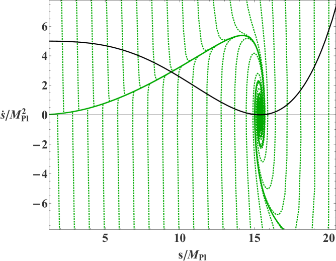
In Fig. 1 we fix the values of the parameters to $\xi=0.3$, $\alpha=0.01$ and $\omega=0.16$, we numerically solve the Klein–Gordon equation (3.17) for a plethora of initial conditions for the inflaton $s$ and plot the $s-\dot{s}$ phase space. Clearly, the potential exhibits an attractor behavior since, regardless of the initial conditions, all trajectories in the phase space (green-dotted curves) quickly converge in a single trajectory that terminates at the location of the minimum.

Figure 1: The attractor behavior of the one-loop effective potential (3.15) in the $s-\dot{s}$ phase space, where we have used $\xi=0.3$, $\alpha=0.01$ and $\omega=0.16$. With the black curve we show the normalized ($5V(s)/V(0)$) potential.

Notice that the conditions (3.2) and (3.12) constrain the free parameters of the model. As a result we find that

$$v_{\phi}^{2}=v^{2}-v_{\zeta}^{2}=6M_{\rm Pl}^{2}\cot^{2}\omega\,.$$ (3.18)

Then, upon substituting (3.12) and (3.18) into (3.2) one obtains

$$2A\cot^{2}\omega=-B\,.$$ (3.19)

Equivalently we have the constraint

$$\left(12\alpha\lambda_{\phi}+6\xi^{2}\right)\cot^{2}\omega=\xi\,,$$ (3.20)

and so we are left with 3 free parameters. If we choose to solve (3.20) for the coupling $\lambda_{\phi}$ we have that

$$\lambda_{\phi}=\frac{\xi}{12\alpha}\left[\tan^{2}\omega-6\xi\right]\,.$$ (3.21)

4 Observables

The imposition of the constraint (3.20), has reduced the number of the free parameters of the system to three, namely the non-minimal coupling of the field ($\xi$), the Starobinsky parameter ($\alpha$), and the mixing angle ($\omega$). As we shall now demonstrate, it is only the angle $\omega$ that affects the predictions for observables and the other two parameters come into play via the VEVs that determine the value of $\omega$.

In the slow-roll approximation, the expressions for the tensor-to-scalar ratio $r$, the tilt $n_{s}$ of the scalar power spectrum and the running $\alpha_{s}$ of the scalar spectral index are given in terms of the values of the potential slow-roll parameters $\epsilon_{V}$, $\eta_{V}$ and $\xi_{V}^{2}$ at horizon crossing as

$$r\approx 16\epsilon_{V}^{*}\,,$$ (4.1)

$$n_{s}\approx 1-6\epsilon_{V}^{*}+2\eta_{V}^{*}\,,$$ (4.2)

and

$$\alpha_{s}=16\epsilon_{V}^{*}\eta_{V}^{*}-24\epsilon_{V}^{2*}-2\xi_{V}^{2*}\ ,$$ (4.3)

where

$$\epsilon_{V}\equiv\frac{M_{\rm Pl}^{2}}{2}\left(\frac{V^{\prime}(s)}{V(s)}\right)^{2}\ ,\quad\eta_{V}\equiv M_{\rm Pl}^{2}\frac{V^{\prime\prime}(s)}{V(s)}\,,\quad\xi^{2}_{V}\equiv M^{4}_{\rm Pl}\frac{V^{\prime}(s)V^{\prime\prime\prime}(s)}{V(s)^{2}}\ ,$$ (4.4)

and ^∗ has been used to denote the value of the slow-roll parameters at horizon crossing.

By performing a direct computation it is straightforward to show that the slow-roll parameters for the potential (3.15) take the form

$$\epsilon_{V}=M_{\rm Pl}^{2}\frac{32s^{6}\,\log{\left[\frac{6M_{\rm Pl}^{2}}{s^{2}\sin^{2}\omega}\right]}\sin^{8}\omega}{\left[36M_{\rm Pl}^{4}+s^{4}\sin^{4}\omega\left(2\log{\left[\frac{s^{2}\sin^{2}\omega}{6M_{\rm Pl}^{2}}\right]}-1\right)\right]^{2}}\ ,$$ (4.5)

$$\eta_{V}=M_{\rm Pl}^{2}\frac{8s^{2}\left[2+3\log{\left(\frac{s^{2}\sin^{2}\omega}{6M_{\rm Pl}^{2}}\right)}\right]\sin^{4}\omega}{36M_{\rm Pl}^{4}+s^{4}\sin^{4}\omega\left(2\log{\frac{s^{2}\sin^{2}\omega}{6M_{\rm Pl}^{2}}}-1\right)}\ ,$$ (4.6)

and

$$\xi_{V}^{2}=M_{\rm Pl}^{4}\frac{128s^{4}\sin^{8}\omega\log\left(\frac{s^{2}\sin^{2}\omega}{6M_{\rm Pl}^{2}}\right)\left(3\log\left(\frac{s^{2}\sin^{2}\omega}{6M_{\rm Pl}^{2}}\right)+5\right)}{\left(s^{4}\sin^{4}\omega\left(2\log\left(\frac{s^{2}\sin^{2}\omega}{6M_{\rm Pl}^{2}}\right)-1\right)+36M_{\rm Pl}^{4}\right)^{2}}\ ,$$ (4.7)

Thus it is evident that the sole parameter that plays a role in the expressions (4.1) and (4.2) for the observables is the mixing angle $\omega$. Note that an inflaton field excursion can occur on either side of the minimum of the potential (3.15), corresponding to small and large field inflation. In the following, however, we will not deal with the large field scenario since it yields a tensor-to-scalar ratio which is excluded by observations.

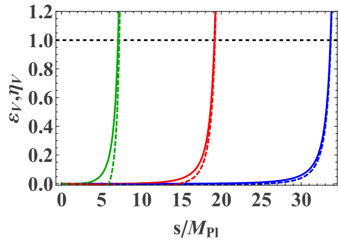
In Fig. 2, we plot the slow-roll parameters $\epsilon_{V}$ and $\eta_{V}$, given in Eqs. (4.5)–(4.6), as a function of the inflaton field $s$ for a few fixed values of the mixing angle $\omega$. We observe that both slow-roll parameters become unity around the same inflaton field value.

Figure 2: The slow-roll parameters $\epsilon_{V}$ (solid curves) and $\eta_{V}$ (dashed curves) as a function of the inflaton field $s$ for fixed values of the mixing angle at $\sin\omega=0.07$ (blue curves), $\sin\omega=0.12$ (red curves) and $\sin\omega=0.30$ (green curves).

The number $N$ of e-folds of inflation elapsed in the Einstein frame is defined as $\text{d}N=H\text{d}t$ where $H$ and $t$ are the Hubble parameter and time coordinate respectively. In terms of the slow roll parameter $\epsilon_{V}$ one has

$$N=\int_{s_{*}}^{s_{f}}\frac{1}{\sqrt{2\epsilon_{V}(s)}}\text{d}s\,,$$ (4.8)

where $s_{*}$ is the value of the inflaton field at the time of horizon crossing while $s_{f}$ is its value at the end of inflation.

In the case of the model under consideration, the total number of e-folds is given by the following analytic expression:

$$N=\left\{\frac{3}{8\sin^{2}\omega}\left[{\rm li}\left(\frac{6\sin^{2}\omega\,M_{\rm Pl}^{2}}{s^{2}}\right)-{\rm li}\left(\frac{\sin^{2}\omega\,s^{2}}{6M_{\rm Pl}^{2}}\right)\right]+\frac{s^{2}}{8M_{\rm Pl}^{2}}\right\}\Bigg{|}_{s_{f}}^{s_{*}}\ ,$$ (4.9)

where ${\rm li}(z)$ is the logarithmic integral (${\rm li}(z)=\int_{0}^{z}\frac{1}{\log t}dt$).

The required amount of inflation in order for the horizon and flatness problems to be solved is $N\approx 60$. Inflation ends exactly when the first Hubble slow-roll parameter $\epsilon_{H}\equiv-\dot{H}/H^{2}=1$ but in the slow-roll approximation $\epsilon_{H}\approx\epsilon_{V}$ and so it is often the condition $\epsilon_{V}=1$ that is used instead in order to obtain $s_{f}$.

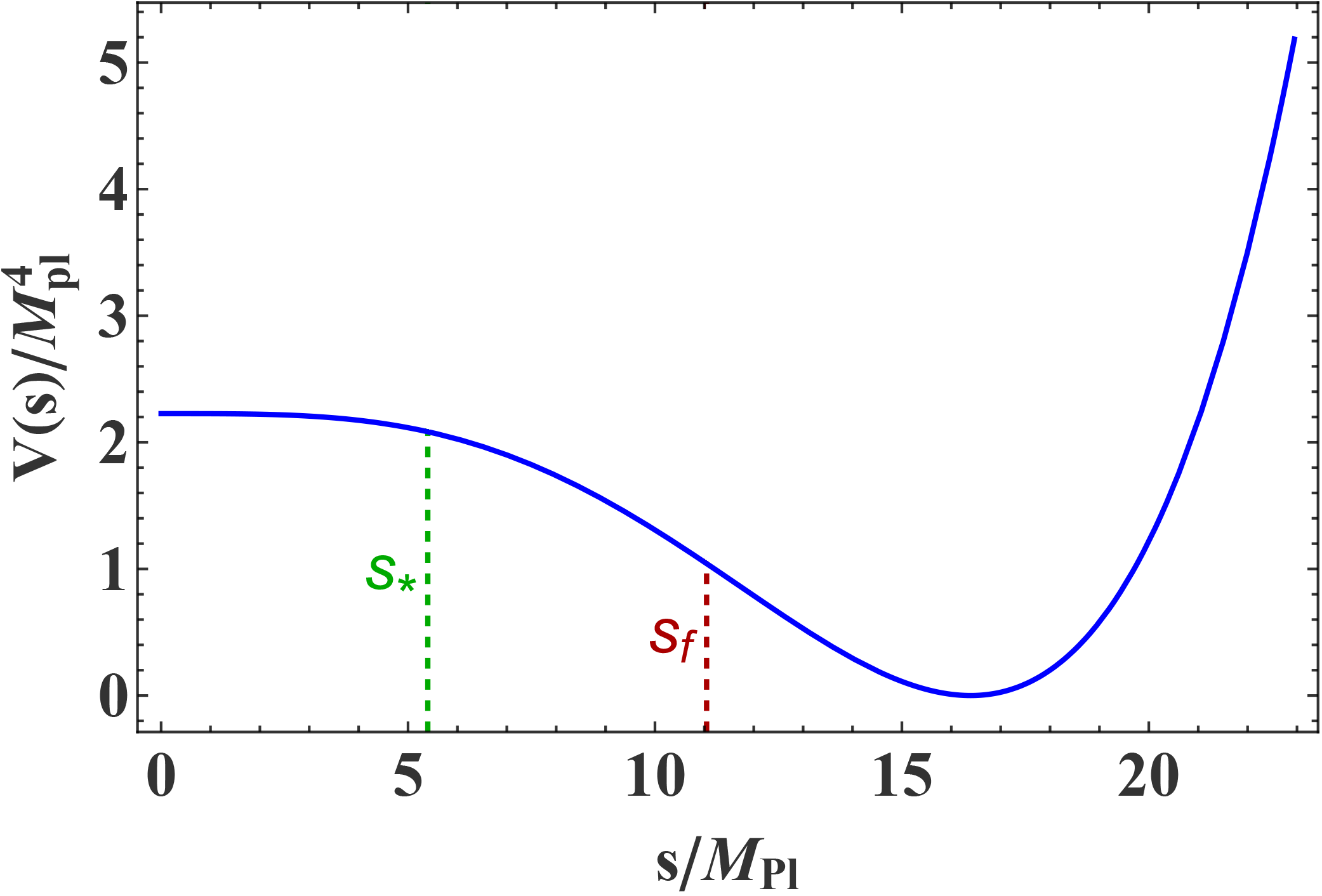
An example of an inflaton excursion in our model (3.15) that yields a sufficient amount of inflation is given in Fig.3. The red-dashed line corresponds to the value $s_{f}$ of the inflaton where inflation ends subject to the condition $\epsilon_{V}=1$. The green-dashed line corresponds to the value $s_{*}$ of the inflaton at the time of horizon crossing that is obtained by the requirement $N\approx 60$.

Figure 3: An inflaton excursion that yields $N=59.3$ when $\sin\omega=0.15$. Inflation starts(ends) at the green(red)-dashed line. The values of the observables in this case are $(r,n_{s})=(0.014,0.963)$.

By considering different values for $s_{*}$ we vary the total number of e-folds of inflation elapsed during the field excursion and consequently obtain different predictions for the observables $r$ and $n_{s}$.

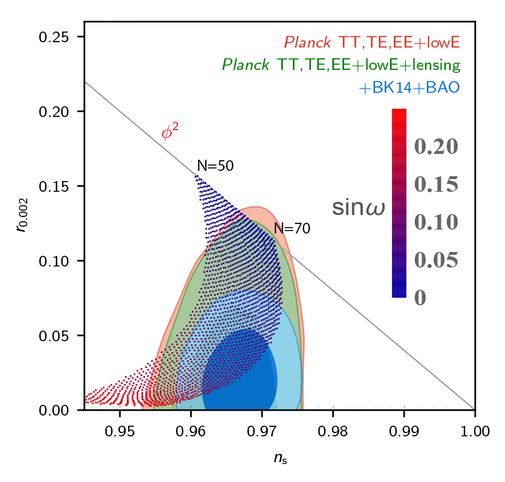
In Fig.4 we considered different values for the mixing angle ranging from $\sin\omega=0$ up to $\sin\omega=0.23$ that yield $50\leqslant N\leqslant 70$ and plot the predictions of the model in the $n_{s}-r$ plane against the current bounds set by the Planck collaboration [8]. One can see that for small values of the mixing angle the predictions of the model converge to the ones obtained by the minimal quadratic inflation model. This is explained by the fact that the potential (3.15), for $\sin\omega\rightarrow 0$ and around its minimum, is approximated by

$$V(s)\simeq\frac{m^{4}_{\sigma}\sin^{2}\omega}{96\pi^{2}M^{2}_{\rm Pl}}\left(s-v_{s}\right)^{2}\ .$$ (4.10)

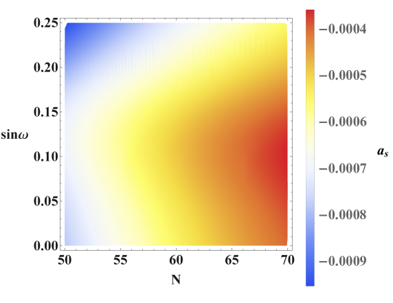
Finally, in Fig. 5, for various values of the mixing angle $\omega$ and for $N=50-70$ e-folds we plot the running of the scalar spectral index $\alpha_{s}$. All of the resulting values are compatible with the observational constraints [8] $\alpha_{s}=-0.0045\pm 0.0067$ at $68\%$ CL.

Figure 4: The predictions of the model (3.15) for a wide range of values for the mixing angle $\omega$ and for field excursions that yield sufficient amount of inflation i.e. 50 to 70 e-folds.

Figure 5: The running of the scalar spectral index $\alpha_{s}$ for values of the mixing angle in the range $\sin\omega=0-0.25$ and for a number of e-folds between $N=50-70$.

5 Summary and Conclusions

In this work, we considered slow-roll inflation in the theory of a scalar field with scale-imvariant interactions coupled to gravity non-minimally in the presence of an $R^{2}$ term. The gravitational sector in the Jordan frame consists of a nonminimal coupling term of the inflaton to the Ricci scalar and an $R^{2}$ correction. Expressing the action in terms of an auxiliary scalar field and transforming it to the Einstein frame by means of a Weyl rescaling of the metric, the theory consists of two real scalar fields with non-canonical kinetic terms subject to a two-dimensional inflationary potential. By applying the formalism of Gildener and Weinberg we were able to effectively describe inflation by means of a single scalar field ($s$), the pseudo-Goldstone boson along the flat direction of the tree-level potential. We obtained the one-loop corrected potential along the flat direction and in turn, by numerically solving the Klein-Gordon equation, we have verified that it exhibits an inflationary attractor behavior.

Then, we studied the predictions for the tensor-to-scalar ratio ($r$), the scalar spectral index ($n_{s}$) and the running of the scalar spectral index ($\alpha_{s}$). We found that the only free parameter that affects the predictions is the mixing angle ($\omega$) between the two scalar degrees of freedom. For various field excursions of the inflaton $s$ that produce a sufficient amount of inflation, i.e. $50$ to $70$ e-folds, and for a wide range of values for $\omega$ we found that the model yields predictions that lie well within the recent, strict bounds for the allowed region in the ($n_{s}-r$) parametric space set by the Planck collaboration. For the aforementioned field excursions and values of the mixing angle the predictions for the running of the spectral index are also in excellent agreement with the observations.

In conclusion, the present model is able to successfully describe inflation and at the same time generate the Planck scale in a dynamical way by means of the Coleman-Weinberg mechanism. The inclusion of the $R^{2}$ term affects mainly the predictions of $r$. Larger values of the Starobinsky coupling $\alpha$ correspond to larger values of the mixing angle $\omega$, which in turn result to smaller values for $r$.

References

- [1] S. W. Hawking, “The Development of Irregularities in a Single Bubble Inflationary Universe,” Phys. Lett. 115B (1982) 295.
- [2] A. A. Starobinsky, “Dynamics of Phase Transition in the New Inflationary Universe Scenario and Generation of Perturbations,” Phys. Lett. 117B (1982) 175–178.
- [3] A. H. Guth and S. Y. Pi, “Fluctuations in the New Inflationary Universe,” Phys. Rev. Lett. 49 (1982) 1110–1113.
- [4] A. D. Linde, “Chaotic Inflation,” Phys. Lett. 129B (1983) 177–181.
- [5] A. A. Starobinsky, “A New Type of Isotropic Cosmological Models Without Singularity,” Phys. Lett. 91B (1980) 99–102.
- [6] V. F. Mukhanov and G. V. Chibisov, “Quantum Fluctuations and a Nonsingular Universe,” JETP Lett. 33 (1981) 532–535. [Pisma Zh. Eksp. Teor. Fiz.33,549(1981)].
- [7] A. A. Starobinsky, “The Perturbation Spectrum Evolving from a Nonsingular Initially De-Sitter Cosmology and the Microwave Background Anisotropy,” Sov. Astron. Lett. 9 (1983) 302.
- [8] Planck Collaboration, Y. Akrami et al., “Planck 2018 results. X. Constraints on inflation,” arXiv:1807.06211 [astro-ph.CO].
- [9] S. Capozziello, S.-i. Nojiri, S. Odintsov, and A. Troisi, “Cosmological viability of f (r)-gravity as an ideal fluid and its compatibility with a matter dominated phase,” Physics Letters B 639 no. 3, (2006) 135–143.
- [10] F. Briscese, E. Elizalde, S. Nojiri, and S. Odintsov, “Phantom scalar dark energy as modified gravity: Understanding the origin of the big rip singularity,” Physics Letters B 646 no. 2, (2007) 105–111.
- [11] S. Nojiri and S. D. Odintsov, “Dark energy, inflation and dark matter from modified f(r) gravity,” 0807.0685v1.
- [12] S. Nojiri and S. D. Odintsov, “Can f(r)-gravity be a viable model: the universal unification scenario for inflation, dark energy and dark matter,” 0801.4843v1.
- [13] A. De Felice and S. Tsujikawa, “f(R) theories,” Living Rev. Rel. 13 (2010) 3, arXiv:1002.4928 [gr-qc].
- [14] S. Capozziello and M. De Laurentis, “Extended Theories of Gravity,” Phys. Rept. 509 (2011) 167–321, arXiv:1108.6266 [gr-qc].
- [15] T. Clifton, P. G. Ferreira, A. Padilla, and C. Skordis, “Modified Gravity and Cosmology,” Phys. Rept. 513 (2012) 1–189, arXiv:1106.2476 [astro-ph.CO].
- [16] M. Rinaldi, G. Cognola, L. Vanzo, and S. Zerbini, “Reconstructing the inflationary from observations,” JCAP 1408 (2014) 015, arXiv:1406.1096 [gr-qc].
- [17] K. Bamba, S. Nojiri, S. D. Odintsov, and D. Sáez-Gómez, “Inflationary universe from perfect fluid and gravity and its comparison with observational data,” Phys. Rev. D90 (2014) 124061, arXiv:1410.3993 [hep-th].
- [18] B. J. Broy, F. G. Pedro, and A. Westphal, “Disentangling the - Duality,” JCAP 1503 no. 03, (2015) 029, arXiv:1411.6010 [hep-th].
- [19] S. D. Odintsov and V. K. Oikonomou, “Inflationary -attractors from gravity,” Phys. Rev. D94 no. 12, (2016) 124026, arXiv:1612.01126 [gr-qc].
- [20] C. Guzzetti, M., N. Bartolo, M. Liguori, and S. Matarrese, “Gravitational waves from inflation,” Riv. Nuovo Cim. 39 no. 9, (2016) 399–495, arXiv:1605.01615 [astro-ph.CO].
- [21] R. V. Wagoner, “Scalar tensor theory and gravitational waves,” Phys. Rev. D1 (1970) 3209–3216.
- [22] T. Damour and G. Esposito-Farese, “Tensor-multi-scalar theories of gravitation,” Classical and Quantum Gravity 9 no. 9, (1992) 2093.
- [23] T. Damour and K. Nordtvedt, “Tensor-scalar cosmological models and their relaxation toward general relativity,” Physical Review D 48 no. 8, (1993) 3436.
- [24] J. D. Barrow, “Slow-roll inflation in scalar-tensor theories,” Physical Review D 51 no. 6, (1995) 2729.
- [25] J. Garcia-Bellido and D. Wands, “Constraints from inflation on scalar - tensor gravity theories,” Phys. Rev. D52 (1995) 6739–6749, arXiv:gr-qc/9506050 [gr-qc].
- [26] H. Boutaleb-Joutei and A. L. Marrakchi, “General scalar-tensor theories for induced gravity inflation,” Nuovo Cim. B112 (1997) 1605–1624.
- [27] B. Boisseau, G. Esposito-Farese, D. Polarski, and A. A. Starobinsky, “Reconstruction of a scalar tensor theory of gravity in an accelerating universe,” Phys. Rev. Lett. 85 (2000) 2236, arXiv:gr-qc/0001066 [gr-qc].
- [28] J. Morris, “Generalized slow-roll conditions and the possibility of intermediate scale inflation in scalar-tensor theory,” Classical and Quantum Gravity 18 no. 15, (2001) 2977.
- [29] G. Esposito-Farese and D. Polarski, “Scalar tensor gravity in an accelerating universe,” Phys. Rev. D63 (2001) 063504, arXiv:gr-qc/0009034 [gr-qc].
- [30] T. Chiba, “1/r gravity and scalar-tensor gravity,” Physics Letters B 575 no. 1, (2003) 1–3.
- [31] A. Stabile, A. Stabile, and S. Capozziello, “Conformal transformations and weak field limit of scalar-tensor gravity,” Physical Review D 88 no. 12, (2013) 124011.
- [32] T. Chiba and M. Yamaguchi, “Conformal-Frame (In)dependence of Cosmological Observations in Scalar-Tensor Theory,” JCAP 1310 (2013) 040, arXiv:1308.1142 [gr-qc].
- [33] Y. N. Obukhov and D. Puetzfeld, “Equations of motion in scalar-tensor theories of gravity: A covariant multipolar approach,” Physical Review D 90 no. 10, (2014) 104041.
- [34] L. Järv, P. Kuusk, M. Saal, and O. Vilson, “Transformation properties and general relativity regime in scalar–tensor theories,” Classical and Quantum Gravity 32 no. 23, (2015) 235013, arXiv:1504.02686 [gr-qc].
- [35] P. Kuusk, L. Jarv, and O. Vilson, “Invariant quantities in the multiscalar-tensor theories of gravitation,” Int. J. Mod. Phys. A31 no. 02n03, (2016) 1641003, arXiv:1509.02903 [gr-qc].
- [36] O. Vilson, “Some remarks concerning invariant quantities in scalar-tensor gravity,” Adv. Appl. Clifford Algebras 27 no. 1, (2017) 321–332, arXiv:1509.02481 [gr-qc].
- [37] G. Tambalo and M. Rinaldi, “Inflation and reheating in scale-invariant scalar-tensor gravity,” Gen. Rel. Grav. 49 no. 4, (2017) 52, arXiv:1610.06478 [gr-qc].
- [38] M. Artymowski and A. Racioppi, “Scalar-tensor linear inflation,” JCAP 1704 no. 04, (2017) 007, arXiv:1610.09120 [astro-ph.CO].
- [39] S. Bhattacharya, K. Das, and K. Dutta, “Attractor Models in Scalar-Tensor Theories of Inflation,” arXiv:1706.07934 [gr-qc].
- [40] K. Bhattacharya and B. R. Majhi, “Fresh look at the scalar-tensor theory of gravity in Jordan and Einstein frames from undiscussed standpoints,” Phys. Rev. D95 no. 6, (2017) 064026, arXiv:1702.07166 [gr-qc].
- [41] D. Burns, S. Karamitsos, and A. Pilaftsis, “Frame-Covariant Formulation of Inflation in Scalar-Curvature Theories,” Nucl. Phys. B907 (2016) 785–819, arXiv:1603.03730 [hep-ph].
- [42] A. Karam, T. Pappas, and K. Tamvakis, “Frame-dependence of higher-order inflationary observables in scalar-tensor theories,” Phys. Rev. D96 no. 6, (2017) 064036, arXiv:1707.00984 [gr-qc].
- [43] S. Karamitsos and A. Pilaftsis, “On the Cosmological Frame Problem,” PoS CORFU2017 (2018) 036, arXiv:1801.07151 [hep-th].
- [44] S. Karamitsos and A. Pilaftsis, “Frame Covariant Nonminimal Multifield Inflation,” Nucl. Phys. B927 (2018) 219–254, arXiv:1706.07011 [hep-ph].
- [45] A. Karam, A. Lykkas, and K. Tamvakis, “Frame-invariant approach to higher-dimensional scalar-tensor gravity,” Phys. Rev. D97 no. 12, (2018) 124036, arXiv:1803.04960 [gr-qc].
- [46] K. Kannike, A. Racioppi, and M. Raidal, “Linear inflation from quartic potential,” JHEP 01 (2016) 035, arXiv:1509.05423 [hep-ph].
- [47] A. Racioppi, “Coleman-Weinberg linear inflation: metric vs. Palatini formulation,” JCAP 1712 no. 12, (2017) 041, arXiv:1710.04853 [astro-ph.CO].
- [48] A. Racioppi, “New universal attractor in nonminimally coupled gravity: Linear inflation,” Phys. Rev. D97 no. 12, (2018) 123514, arXiv:1801.08810 [astro-ph.CO].
- [49] A. Karam, L. Marzola, T. Pappas, A. Racioppi, and K. Tamvakis, “Constant-Roll (Quasi-)Linear Inflation,” JCAP 1805 no. 05, (2018) 011, arXiv:1711.09861 [astro-ph.CO].
- [50] M. Artymowski, Z. Lalak, and M. Lewicki, “Inflationary scenarios in Starobinsky model with higher order corrections,” JCAP 1506 (2015) 032, arXiv:1502.01371 [hep-th].
- [51] C. van de Bruck and L. E. Paduraru, “Simplest extension of Starobinsky inflation,” Phys. Rev. D92 (2015) 083513, arXiv:1505.01727 [hep-th].
- [52] T. Asaka, S. Iso, H. Kawai, K. Kohri, T. Noumi, and T. Terada, “Reinterpretation of the Starobinsky model,” PTEP 2016 no. 12, (2016) 123E01, arXiv:1507.04344 [hep-th].
- [53] M. Artymowski, Z. Lalak, and M. Lewicki, “Saddle point inflation from higher order corrections to Higgs/Starobinsky inflation,” Phys. Rev. D93 no. 4, (2016) 043514, arXiv:1509.00031 [hep-th].
- [54] S. Kaneda and S. V. Ketov, “Starobinsky-like two-field inflation,” Eur. Phys. J. C76 no. 1, (2016) 26, arXiv:1510.03524 [hep-th].
- [55] X. Calmet and I. Kuntz, “Higgs Starobinsky Inflation,” Eur. Phys. J. C76 no. 5, (2016) 289, arXiv:1605.02236 [hep-th].
- [56] C. van de Bruck, P. Dunsby, and L. E. Paduraru, “Reheating and preheating in the simplest extension of Starobinsky inflation,” Int. J. Mod. Phys. D26 no. 13, (2016) 1750152, arXiv:1606.04346 [gr-qc].
- [57] Y.-C. Wang and T. Wang, “Primordial perturbations generated by Higgs field and operator,” Phys. Rev. D96 no. 12, (2017) 123506, arXiv:1701.06636 [gr-qc].
- [58] Y. Ema, “Higgs Scalaron Mixed Inflation,” Phys. Lett. B770 (2017) 403–411, arXiv:1701.07665 [hep-ph].
- [59] T. Mori, K. Kohri, and J. White, “Multi-field effects in a simple extension of inflation,” JCAP 1710 no. 10, (2017) 044, arXiv:1705.05638 [astro-ph.CO].
- [60] S. Pi, Y.-l. Zhang, Q.-G. Huang, and M. Sasaki, “Scalaron from -gravity as a heavy field,” JCAP 1805 no. 05, (2018) 042, arXiv:1712.09896 [astro-ph.CO].
- [61] M. He, A. A. Starobinsky, and J. Yokoyama, “Inflation in the mixed Higgs- model,” JCAP 1805 no. 05, (2018) 064, arXiv:1804.00409 [astro-ph.CO].
- [62] D. Gorbunov and A. Tokareva, “Scalaron the healer: removing the strong-coupling in the Higgs- and Higgs-dilaton inflations,” arXiv:1807.02392 [hep-ph].
- [63] D. M. Ghilencea, “Two-loop corrections to Starobinsky-Higgs inflation,” arXiv:1807.06900 [hep-ph].
- [64] S.-J. Wang, “Quintessential Starobinsky inflation and swampland criteria,” arXiv:1810.06445 [hep-th].
- [65] I. Antoniadis, A. Karam, A. Lykkas, and K. Tamvakis, “Palatini inflation in models with an term,” arXiv:1810.10418 [gr-qc].
- [66] A. Gundhi and C. F. Steinwachs, “Scalaron-Higgs inflation,” arXiv:1810.10546 [hep-th].
- [67] F. Cooper and G. Venturi, “Cosmology and Broken Scale Invariance,” Phys. Rev. D24 (1981) 3338.
- [68] M. Shaposhnikov and D. Zenhausern, “Scale invariance, unimodular gravity and dark energy,” Phys. Lett. B671 (2009) 187–192, arXiv:0809.3395 [hep-th].
- [69] J. Garcia-Bellido, J. Rubio, M. Shaposhnikov, and D. Zenhausern, “Higgs-Dilaton Cosmology: From the Early to the Late Universe,” Phys. Rev. D84 (2011) 123504, arXiv:1107.2163 [hep-ph].
- [70] V. V. Khoze, “Inflation and Dark Matter in the Higgs Portal of Classically Scale Invariant Standard Model,” JHEP 11 (2013) 215, arXiv:1308.6338 [hep-ph].
- [71] F. Bezrukov, G. K. Karananas, J. Rubio, and M. Shaposhnikov, “Higgs-Dilaton Cosmology: an effective field theory approach,” Phys. Rev. D87 no. 9, (2013) 096001, arXiv:1212.4148 [hep-ph].
- [72] E. Gabrielli, M. Heikinheimo, K. Kannike, A. Racioppi, M. Raidal, and C. Spethmann, “Towards Completing the Standard Model: Vacuum Stability, EWSB and Dark Matter,” Phys. Rev. D89 no. 1, (2014) 015017, arXiv:1309.6632 [hep-ph].
- [73] A. Salvio and A. Strumia, “Agravity,” JHEP 06 (2014) 080, arXiv:1403.4226 [hep-ph].
- [74] C. Csaki, N. Kaloper, J. Serra, and J. Terning, “Inflation from Broken Scale Invariance,” Phys. Rev. Lett. 113 (2014) 161302, arXiv:1406.5192 [hep-th].
- [75] K. Kannike, G. Hütsi, L. Pizza, A. Racioppi, M. Raidal, A. Salvio, and A. Strumia, “Dynamically Induced Planck Scale and Inflation,” JHEP 05 (2015) 065, arXiv:1502.01334 [astro-ph.CO].
- [76] A. O. Barvinsky, A. Yu. Kamenshchik, and D. V. Nesterov, “Origin of inflation in CFT driven cosmology: -gravity and non-minimally coupled inflaton models,” Eur. Phys. J. C75 no. 12, (2015) 584, arXiv:1510.06858 [hep-th].
- [77] L. Marzola and A. Racioppi, “Minimal but non-minimal inflation and electroweak symmetry breaking,” JCAP 1610 no. 10, (2016) 010, arXiv:1606.06887 [hep-ph].
- [78] N. D. Barrie, A. Kobakhidze, and S. Liang, “Natural Inflation with Hidden Scale Invariance,” Phys. Lett. B756 (2016) 390–393, arXiv:1602.04901 [gr-qc].
- [79] L. Marzola, A. Racioppi, M. Raidal, F. R. Urban, and H. Veermäe, “Non-minimal CW inflation, electroweak symmetry breaking and the 750 GeV anomaly,” JHEP 03 (2016) 190, arXiv:1512.09136 [hep-ph].
- [80] M. Rinaldi and L. Vanzo, “Inflation and reheating in theories with spontaneous scale invariance symmetry breaking,” Phys. Rev. D94 no. 2, (2016) 024009, arXiv:1512.07186 [gr-qc].
- [81] A. Farzinnia and S. Kouwn, “Classically scale invariant inflation, supermassive WIMPs, and adimensional gravity,” Phys. Rev. D93 no. 6, (2016) 063528, arXiv:1512.05890 [hep-ph].
- [82] G. K. Karananas and J. Rubio, “On the geometrical interpretation of scale-invariant models of inflation,” Phys. Lett. B761 (2016) 223–228, arXiv:1606.08848 [hep-ph].
- [83] P. G. Ferreira, C. T. Hill, and G. G. Ross, “Scale-independent inflation and hierarchy generation,” Physics Letters B 763 (2016) 174–178.
- [84] K. Kannike, M. Raidal, C. Spethmann, and H. Veermäe, “The evolving Planck mass in classically scale-invariant theories,” JHEP 04 (2017) 026, arXiv:1610.06571 [hep-ph].
- [85] P. G. Ferreira, C. T. Hill, and G. G. Ross, “Weyl Current, Scale-Invariant Inflation and Planck Scale Generation,” Phys. Rev. D95 no. 4, (2017) 043507, arXiv:1610.09243 [hep-th].
- [86] A. Salvio, “Inflationary Perturbations in No-Scale Theories,” Eur. Phys. J. C77 no. 4, (2017) 267, arXiv:1703.08012 [astro-ph.CO].
- [87] K. Kannike, A. Racioppi, and M. Raidal, “Super-heavy dark matter – Towards predictive scenarios from inflation,” Nucl. Phys. B918 (2017) 162–177, arXiv:1605.09378 [hep-ph].
- [88] A. Barnaveli, S. Lucat, and T. Prokopec, “Inflation as a spontaneous symmetry breaking of Weyl symmetry,” arXiv:1809.10586 [gr-qc].
- [89] P. G. Ferreira, C. T. Hill, J. Noller, and G. G. Ross, “Inflation in a scale invariant universe,” Phys. Rev. D97 no. 12, (2018) 123516, arXiv:1802.06069 [astro-ph.CO].
- [90] S. R. Coleman and E. J. Weinberg, “Radiative Corrections as the Origin of Spontaneous Symmetry Breaking,” Phys. Rev. D7 (1973) 1888–1910.
- [91] E. Gildener and S. Weinberg, “Symmetry Breaking and Scalar Bosons,” Phys. Rev. D13 (1976) 3333.
- [92] R. H. Dicke, “Mach’s principle and invariance under transformation of units,” Physical Review 125 no. 6, (1962) 2163.
- [93] J. C. Hwang, “Cosmological perturbations in generalized gravity theories: Formulation,” Class. Quant. Grav. 7 (1990) 1613–1631.
- [94] J.-c. Hwang, “Cosmological perturbations in generalized gravity theories: Conformal transformation,” Class. Quant. Grav. 14 (1997) 1981–1991, arXiv:gr-qc/9605024 [gr-qc].