Regressive and generative neural networks for scalar field theory
Abstract
We explore the perspectives of machine learning techniques in the context of quantum field theories. In particular, we discuss two-dimensional complex scalar field theory at nonzero temperature and chemical potential – a theory with a nontrivial phase diagram. A neural network is successfully trained to recognize the different phases of this system and to predict the value of various observables, based on the field configurations. We analyze a broad range of chemical potentials and find that the network is robust and able to recognize patterns far away from the point where it was trained. Aside from the regressive analysis, which belongs to supervised learning, an unsupervised generative network is proposed to produce new quantum field configurations that follow a specific distribution. An implicit local constraint fulfilled by the physical configurations was found to be automatically captured by our generative model. We elaborate on potential uses of such a generative approach for sampling outside the training region.
I Introduction
Deep learning with a hierarchical structure of artificial neural networks is a branch of machine learning aiming at understanding and extracting high-level representations of big data Hinton:2015nature . It is particularly effective in tackling complex non-linear systems with a high level of correlations that cannot be captured easily by conventional techniques. Traditionally employed for tasks like pattern recognition in images or speech, automated translation or board game-playing, applications of deep learning have been found recently in many areas of physics including nuclear Pang:2016vdc ; Utama:2017ytc ; Bayram:2018gqi ; Neufcourt:2018syo , particle Baldi:2014kfa ; Baldi:2014pta ; Barnard:2016qma ; Moult:2016cvt ; Radovic:2018dip and condensed matter 2016PhRvB..94s5105W ; 2017NatPh..13..435V ; 2017PhRvX…7c1038C ; 2017NatSR…7.8823B ; 2017NatPh..13..431C ; Carleo602 ; 2017PhRvB..95d1101L ; 2016PhRvB..94p5134T ; 2017PhRvB..95c5105H ; PhysRevX.8.031012 physics.
Significant progress has been made in utilizing machine learning methods for condensed matter systems like classical or quantum spin models. Specific tasks in these settings include the discrimination between certain phases and the identification of phase transitions 2016PhRvB..94s5105W ; 2017NatPh..13..435V ; 2017PhRvX…7c1038C ; 2017NatSR…7.8823B ; 2017NatPh..13..431C , the compressed representation of quantum wave functions Carleo602 or the acceleration of Monte-Carlo algorithms 2017PhRvB..95d1101L ; 2016PhRvB..94p5134T ; 2017PhRvB..95c5105H . Recently, deep neural networks have also been considered in particle physics, for the processing of experimental heavy-ion collision datasets Pang:2016vdc and in the context of algorithmic development for numerical lattice field theory simulations Mori:2017nwj ; Shanahan:2018vcv ; Tanaka:2017niz .
Pattern recognition, especially classification and regression tasks, have been discussed previously in interacting many-body systems for condensed matter physics. In the present paper, we generalize the application of deep learning for the classification of phases in a lattice quantum field theoretical setting. We further demonstrate the capability of deep neural networks in learning physical observables, even with highly non-linear dependence on the field configurations and with only limited training data – providing an effective high-dimensional non-linear regression method. In addition, we proceed by implementing, for the first time, a Generative Adversarial Network (GAN) NIPS2014_5423 for lattice field theory in order to generate field configurations following and generalizing the training set distribution. This is an unsupervised learning framework that uses unlabeled data to perform representation learning. Such a GAN-powered approach is not a full-fledged alternative to the Monte-Carlo algorithm, which possesses desired properties like ergodicity, reversibility and detailed balance. However, it can result in a one-pass direct sampling network where no Markov chain is needed. Our aim here is to provide a proof of principle that generative networks, if trained adequately, are capable of capturing and representing the distribution of configurations in a strongly correlated quantum field theory. On the practical side, generative networks would prove useful when combined with traditional approaches to accelerate simulation algorithms, e.g., by improving decorrelation for proposals in a Markov chain process. Further potential use of such setups would be for reducing large ensembles of field configurations into a single (highly trained) network as an efficient representation for the quantum statistical field ensembles, thereby significantly reducing storage requirements.
Specifically, we consider two-dimensional quantum scalar field theory discretized on a lattice, and implement a deep neural network for the investigation of field configurations generated via standard Monte-Carlo algorithms. We aim at testing whether the machine is capable of recognizing known features of the system including phase transitions and the corresponding behavior of various observables. More interestingly, we also look for hidden patterns discovered by the network, i.e. correlations of the gross features of the system with further low-level variables. Furthermore, we explore the approach of generating field configurations using GAN and reproducing physical distributions.
This paper is structured as follows. In Sec. II we outline the scalar field theory setup, including the details of the configuration space and the definition of the observables. This is followed by Sec. III, where we describe our neural network hierarchy and discuss the classification and regression tasks, together with the details of the generative network approach. In Sec. IV we summarize our main findings and conclude. Two appendices contain the details of the dualization of scalar field theory (App. A) and the specifications of the GAN approach (App. B).
II Observables in scalar field theory
We consider a complex scalar field with mass and quartic coupling in dimensional Euclidean space-time at nonzero temperature . This system is studied in the grand canonical approach, introducing a chemical potential that controls how the charge density fluctuates. For low temperatures, two different regimes of the parameter space can be distinguished: At low the density is suppressed, usually referred to as the Silver Blaze behavior PhysRevLett.91.222001 , whereas above a threshold the density increases considerably.111In the following we will refer to the pronounced change in the density at the threshold as a transition, keeping in mind that – in accordance with the Mermin-Wagner theorem – it is not connected to spontaneous symmetry breaking. People conjecture that the QCD phase diagram also holds such a behavior in the region at low temperatures and medium to high densities PhysRevLett.91.222001 .
This interesting behavior is a non-perturbative phenomena and cannot be observed directly, as the action becomes complex for , hindering standard simulations in terms of the field . However, using the worldline formalism, the partition function can be reexpressed using dual variables and the action rendered real and positive Gattringer:2012df , see details in App. A. The dual variables are the integers and that are associated to the links starting at the point and lying in the direction (space) or (time). The total number of variables is therefore , where denotes the number of lattice sites in the direction . The partition function becomes a sum over this -dimensional configuration space,
| (1) |
with the lattice action described in Eq. (8). While the -integers can take arbitrary values, the -integers satisfy a zero divergence-type constraint,
| (2) |
where is the unit vector in the direction and the lattice spacing.
The partition function (1) contains all information about the system. In particular, the expectation values of the particle density and of the squared field are related to derivatives of with respect to , and to , respectively. Using the explicit form of the action (8), the corresponding operators read
| (3) | ||||
| (4) |
where the weight and the function are defined in Eq. (9).
Summarizing, in our representation of complex scalar field theory, one field configuration consists of integers and and the path integral is a sum over these field configurations, generated with the appropriate probabilities. The observables on a given configuration are obtained according to Eqs. (3)-(4). This is a simple sum over the variables for the density and a highly nonlinear function for the squared field operator that depends on all and variables, see (9).
We consider a low-temperature ensemble (the dimensionality of the configuration space is therefore ) generated with mass , coupling and a range of chemical potentials around the threshold value (all dimensionful quantities are understood in lattice units). For , is almost zero and is constant. In contrast, both observables rise approximately linearly beyond the threshold. This is demonstrated in Fig. 1.
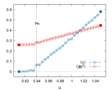
An additional remark about the density operator (3) is in order. Due to the constraint (2), the variables always form closed loops. The contribution of such loops to depends on how many times the loop winds around the direction. Therefore, the density operator may only assume times integer values on any configuration. For the presently investigated lattice geometry this means that is an integer multiple of . Note that this discreteness of the density is a finite volume artifact and becomes continuous in the thermodynamic limit.
III Scalar field theory in a neural network
In the present work we apply deep neural networks for the complex scalar field configurations generated with the dualization approach using standard Monte-Carlo methods, as described in Sec. II. Specifically, the lattice configurations consisting of integers are considered as input to the machine. We investigated the ability of the neural network to perform different tasks including phase transition detection and physical observable regression. Finally we propose a new configuration generation method using the Generative Adversarial Network (GAN) approach.
III.1 Classification of phases
We first employ the network to detect the transition between the low- and high-density phases of the system by performing a classification task. In particular, we train the neural network to identify the threshold chemical potential without specific physical guidance. The recognition of high-level abstract patterns in the data is essential for this classification, thus we consider a Convolutional Neural Network (CNN), which is usually designed for such tasks. We train a CNN to target at a binary classification: The configurations are either in the low-density “Silver Blaze” region () or in the condensed region (). To perform a semi-supervised training, we feed the lattice configurations at and at as input to the CNN network which has a topology as shown in Fig. 2. The training points are also highlighted in Fig. 1.
The input configurations are viewed as images with 4 channels representing the 4 integer field variables (, , and ) and lattice size . We use three convolutional layers each followed by average pooling (except for the first convolutional layer, see in Fig. 2), batch normalization (BN), dropout and PReLU activation. In the first convolutional layer there are 16 filters of size scanning through the input configuration images and creating 16 feature maps of size . After BN and PReLU activation, these feature maps are further convoluted in the second convolutional layer with 32 filters of size . The output from second convolutional layer are half pooled by a subsequent average pooling layer before further processing. Dropout is applied after the final convolutional layer and in between the first two fully-connected layers. The weight matrix of both convolutional layers are initialized with normal distribution and constrained with regularization. In a convolutional layer, each neuron only locally connects to a small chunk of neurons in the previous layer by a convolution operation — this is a key reason for the success of the CNN architecture. After the third convolutional layer and a second average pooling the resulting 32 feature maps of size are flattened and connected to a 256-neuron fully connected layer with batch normalization, dropout and PReLU activation. The final output layer is another fully connected layer with softmax activation and 2 neurons to indicate the two configuration classes. Dropout, batch normalization, PReLU and regularization work together to prevent overfitting that may hinder the generalization ability of the network.

Supervised learning is applied here for this binary classification problem, where the configurations at are labelled as and the ones at as in the training dataset. The cross entropy between the true label and the network output (binary vector), which can quantify well the difference for distributions, is taken as the loss function for training the network where represents the trainable parameters of the neural network. Learning/Training is performed by updating to minimize the loss function, where is the learning rate with initial value 0.0001 and adaptively changed using the AdaMax method. The training data set consists of 30,000 configuration samples for each class and fed into the network in batches with batch size selected to be 16. 20% of the training set are randomly chosen to serve as validation set. In our study, the training runs for 1000 epochs for the neural network, during which the model parameters are saved to a new checkpoint whenever a smaller validation error is encountered. Small fluctuations of validation accuracy are observed to saturate at around 99%.
Once trained, we test the CNN by scanning through the configurations at different values of the chemical potential . The output of the network for each configuration is identified as the probability that the configuration in question corresponds to the condensed phase. In Fig. 3 we show predicted by the network as a function of various quantities: the chemical potential, the number density and the squared field. Looking at in the left panel of the figure, we observe that while for low/high chemical potentials the configurations unambiguously fall in one of the two classes (/), the ensembles at intermediate contain configurations from both sectors. This expresses the enhanced fluctuations in the vicinity of , as expected near a transition.
To understand what the deep neural network has learned for its decision making on phase classification, we can investigate the correlation between neural network’s output and physical observables. Indeed, much more interesting trends are visible in the plots showing as a function of and of as shown in Fig. 3 (middle and right panels). The network outputs are strongly correlated with and . Without any specific supervision to the network about their role, the CNN has clearly learned the relevance of these observables for the transition. In other words, the designed CNN managed to identify highly non-linear features in the configurations that correspond to the physical observables (3) and (4). Particularly for the number density , we see that its non-zero value is perfectly indicated by the non-zero probability from the trained network.
We mention that we also tried reducing the number of convolutional layers in the network to two. In this case we observed similar signals for with slightly worse performance.
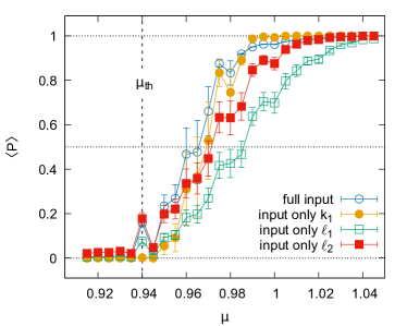
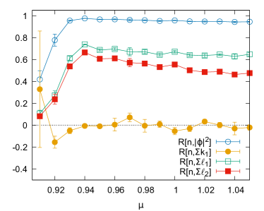
As can be read off from Eq. (3), the particle number is given by the sum of all the variables. This simple pattern might be easily learned by the network. We thus performed the same binary classification task with a restricted training input, including only one of the remaining three variable sets: either , or . The results for the three restricted inputs, together with the full input, are visualized in Fig. 4, plotting the expectation value of the network predicted condensation probability against the chemical potential. Clearly, the network succeeded in learning essentially the same features also using the restricted inputs, as starts to rise at around the same threshold chemical potential for all four cases. This inspires us to analyze the correlation between the number density and the similarly defined observables involving either , or . To this end we consider the normalized correlation coefficient
| (5) |
which vanishes for decorrelated data and equals unity for complete correlation. As shown in Fig. 5, , and also are all strongly correlated with , while is fully decorrelated. Still, the machine succeeds in classifying the configurations based only on , as indicated in Fig. 4. Note that with conventional techniques, neither of the physical observables (3)-(4) sensitive to the transition can be constructed using only the variables. The excellent performance of our CNN, shown in Fig. 4, indicates the existence of strong hidden features in the variables that correlate with the phase of the system. According to these results, the network has the ability to decode these hidden correlations in a highly effective manner.
III.2 Non-linear regression of observables
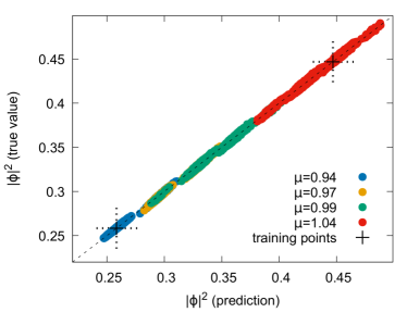
Next, we consider a regression task for learning thermodynamic observables of the system, employing a similar training strategy as used above for the binary classification. In particular, supervised learning is applied with a CNN to regress the thermodynamic observables including the particle number density and the squared field, based on the lattice configurations. As in Sec. III.1, the training dataset consists of configurations at and . The generalization ability of the machine is investigated by testing the network predictions on configurations at intermediate values of the chemical potential.
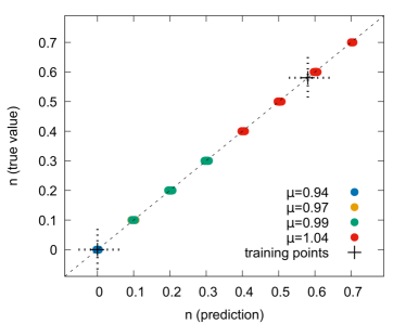
To target this regression task, we change the CNN architecture slightly. Specifically, the batch normalization and pooling layers are removed, and one more fully connected layer with 32 neurons is inserted before the final output layer. The latter consists of 2 neurons representing the values of and of . The activation functions are all changed to ReLU and the loss function for the network is chosen to be the mean squared difference between the predictions and the true values. After 2000 epochs of training, our regression network is tested on previously unseen configurations at different values of the chemical potential. The results for the density and for the squared field are plotted in Fig. 6, showing the true values of the observables, calculated using Eqs. (3)-(4), against the network predictions.
As visible in Fig. 6, the network performs well over a broad range of chemical potentials, predicting and accurately, the maximal deviation being around for the density and around for the squared field. Note that the training was performed using only two far-away segments of the range of the target observables, corresponding to configurations at and (the expectation values of the observables for these ensembles are also indicated in the plots). On the one hand, the high quality of the regression for the density may seem natural owing to the linear dependence (3) of on the individual variables. On the other hand, the squared field is a highly non-linear function of the high-dimensional input (), making the excellent predictive ability of the network very non-trivial and surprising. Put differently, using limited training data (covered small range of the target domain), our CNN network has the ability to correctly reproduce the whole target space mapping, which is curved and even dramatically changing (close to transition point). This means that the network has effectively encoded the configuration into a much plainer and abstract latent space (intermediate layers inside the network). A linear interpolation in these layers can result in non-linear regression in the final output layer.
Just as the middle panel of Fig. 4, the upper panel of Fig. 6 reflects the discreteness of the density operator , evaluated on any configuration. Notice that while the true values of are indeed integer multiples of , small deviations (below in magnitude) from this rule occur for the predicted values. Such deviations stem from the approximative nature of the regression network and are observed to decrease as the number of training epochs is increased. We get back to this behavior below in the generative network analysis.
III.3 Configuration production using the Generative Adversarial Network
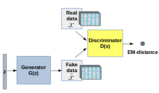
Generative Adversarial Network (GAN) NIPS2014_5423 is a deep generative model that aims to learn the distribution of input variables from the training data. It belongs to the unsupervised learning category within deep learning approaches. The GAN framework contains two non-linear differentiable functions, both of which are represented by adaptive deep neural networks. The first one is the generator , which maps random noise vectors from a latent space with distribution (usually uniform or normal distribution over ) to the target data space with implicit distribution (over data ) that approaches the desired distribution through training. The second one is the discriminator with a single scalar output, which tries to distinguish real data from generated data . These two neural networks are trained alternately, thus improving their respective abilities against each other in a two-player minimax game (also called zero-sum game). An optimally trained GAN converges to the state (the Nash equilibrium for this game-theory problem), where the generator excels in ‘forging’ samples that the discriminator cannot anymore distinguish from real data. Such generative modeling-assisted approaches have been tested in various scientific contexts, including medicine DBLP:journals/corr/NieTPRS16 ; Mahapatra2017ImageSR , particle physics deOliveira:2017pjk ; Paganini:2017dwg ; Paganini:2017hrr , cosmology Ravanbakhsh:2016xpe ; 2017MNRAS.467L.110S ; 2017arXiv170602390M and condensed matter physics PhysRevE.96.043309 ; PhysRevE.97.032119 . Here we employ, for the first time, the generative modeling GAN application in strongly correlated quantum field theory. To ensure training stability, we consider the Wasserstein-GAN architecture 2017arXiv170107875A with gradient penalty (WGAN-gp) 2017arXiv170400028G in this study, see Fig. 7 for the main architecture. The theoretical foundations of WGAN are outlined in App. B.
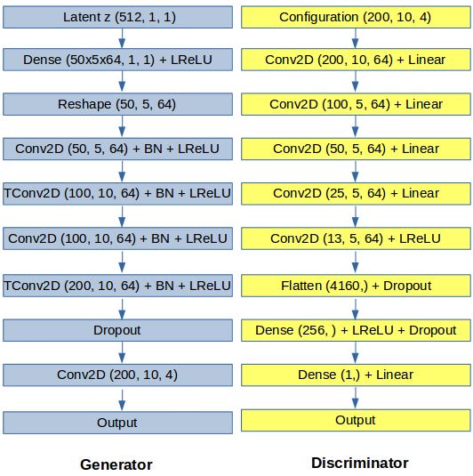
The generator and discriminator architectures are illustrated in Fig. 8. The generator takes as input a randomly sampled 512-dimensional latent vector following a multivariate normal Gaussian distribution, and gradually transforms to the desired configuration space (of dimensionality ). The up-sampling is done via transposed convolution, which is also known as fractionally-strided convolution that function backward the convolution operation. The kernel size for the convolutional layer is , while for the transposed convolutional layer . Batch normalization is included to standardize the outputs and to stabilize training. Apart from the last layer we use the Leaky Rectified Linear Unit (LReLU) as activation function. The discriminator aims to evaluate the ‘fidelity’ of the configurations. The difference between the output of real data and fake data is quantified using the Earth Mover (EM)-distance (also called Wasserstein distance), which serves as the loss function here. Strided convolution is performed for the down-sampling. Note that for the first four convolutional layers plain linear activation is used to let the discriminator more effectively reduce the dimensionality of the input configurations (function like PCA). This helps the GAN to capture the implicit multimodal distribution (of physical observables), as we will see below.
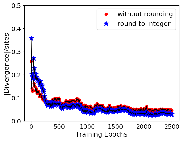
Having trained the GAN, the generator can be used to convert samples from the prior distribution to data points lying in configuration space. To verify the effectiveness of the network and, in particular, whether the generated configurations are indeed physical, we will first check the divergence-type constraint (2) for the complex scalar field. As shown in Fig. 9, the absolute divergence per site for the generated outputs is not exactly zero but is decreasing and converges to zero as the number of training epochs grows. Note that Eq. (2) represents a highly implicit physical constraint inside the training dataset, which is not provided as supervision to the training of the GAN. Instead, the network automatically recognized this constraint for the configurations in a converging way. The generation time for a single configuration using the GAN (on an Nvidia TitanXp GPU) is .
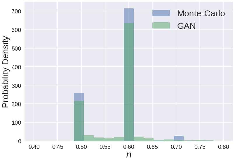
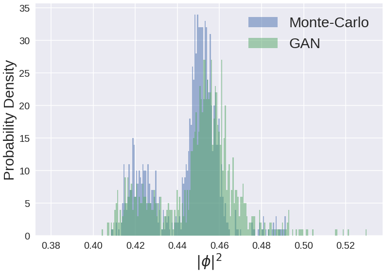
Next we turn to the distribution of observables in the samples generated by the GAN and check to what extent it agrees with the training distribution. In the top panel of Fig. 10 we visualize the probability density distribution of the number density from the GAN after training with one ensemble of configurations at . We observe that the GAN has captured the discrete distribution of quite well. The ensemble average of the particle number density from GAN is estimated (using 1000 random samples) to be , also quite close to the Monte-Carlo value . As mentioned earlier, the particle number density (3) is simply the sum of time component of the variables in the configuration. In contrast, the squared field calculated using Eq. (4) is highly non-linear in the input variables. Nevertheless, the multi-modal distribution of is also well reproduced by the generative network, see the bottom panel of Fig. 10. The ensemble average of from GAN (for the same 1000 samples above) , is also close to the Monte-Carlo result . Figs. 9 and 10 clearly demonstrate that the generative adversarial network can be trained to capture the statistical distribution of the field configurations even on the level of physical observables.
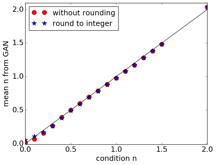
The above GAN structure is designed to reproduce certain distributions in the training dataset. Next we attempt to use the network to generalize the distribution that it was trained on. The discriminator is provided with relevant labels (in this case the value of the number density ) for the training dataset in order to condition the network (cGAN) DBLP:journals/corr/MirzaO14 . Specifically, the training sample at contains cases , , and . After the training we test the generalization ability of the network by specifying desired number densities outside the above set of values. Fig. 11 shows the performance of the cGAN for this generalization task. We stress that for the training only values were provided, but the agreement between the desired (condition) and the measured on the generated configurations is spectacular over a much broader range of density values. This generalization task might be viewed as converting the grand-canonical ensemble of configurations (at fixed ) to a series of canonical ensembles (at various values of ).
IV Conclusions
In this paper we proposed a set of novel techniques for the investigation of a lattice-regularized quantum field theory by means of deep neural networks, including discovering hidden correlations, learning observables and producing field configurations. Specifically, our analysis was carried out for the dualized representation of complex scalar field theory in 1+1 dimensions.
We first showed that a convolutional neural network can be used in a semi-supervised manner to detect the phase transition in this strongly correlated quantum field theory based on the microscopic configurations. We found that the network is capable of recognizing correlations in the system between various observables and phases classification without the specific knowledge guidance. Very interestingly, the network discovered a correlation beyond the conventional analysis, which enabled it to use a restricted subset of the input variables (in particular, the variables) alone to decode information about the phase transition.
We continued by designing a regressive neural network to learn physical observables ( and ) with limited training samples. The network achieved remarkable agreement with the physical observables and also revealed a great generalization ability when tested at chemical potentials beyond the training set. This approach provides an effective high-dimensional non-linear regression method even with limited (compared to the huge Hilbert space, i.e. number of possible configurations) data points, where traditional interpolation or regression would require much higher statistics that grows exponentially with input dimensionality.
Finally, we proposed to generate new configurations following a specific distribution by adapting the modern deep generative modeling technique GAN. We found that the generator in the GAN has the ability of automatically recognizing the implicit but crucial physical constraint on the configurations in an unsupervised manner, and can represent the distribution of prominent observables with direct sampling. The generalization of configuration production to different parameter domains, e.g. towards a critical region, where conventional techniques slow down considerably, is clearly a fascinating feature that deserves further investigations.
Acknowledgements.
This work is supported by the funding of AI research at FIAS from SAMSON AG Frankfurt (K.Z.), DFG Emmy Noether Programme EN 1064/2-1 (G.E.), NSF JETSCAPE ACI-1550228 (L.-G.P.), endowment through the Judah M. Eisenberg Laureatus Chair at Goethe University and the Walter Greiner Gesellschaft at Frankfurt (H.St.). K.Z. gratefully acknowledges supports from the NVIDIA Corporation with the donation of NVIDIA TITAN Xp GPU cards for the research. G.E. acknowledges inspiring discussions with Gábor Varga.Appendix A Dual formulation of scalar field theory
In the continuum, the Euclidean action of a complex 1+1-dimensional scalar field reads
| (6) |
where the covariant derivative is , denotes the mass of the charged scalar field, the quartic coupling and the chemical potential. The spatial () and time-like () coordinates are labelled by . In Eq. (6), denotes the spatial extent of the system and the temperature and we use periodic boundary conditions in both directions.
On a lattice with spacing , the derivative operator is discretized by nearest-neighbor hoppings. The chemical potential assigns different weights to forward and backward hoppings in the time-like direction so that the regularization of the continuum action is
| (7) |
where labels the lattice sites that range over . The lattice sizes are related to the volume and the temperature as and . The partition function of this system is defined by the path integral (1) over the (complex) field configurations.
The chemical potential spoils the reality of so that for we face a complex action problem that leads to a highly oscillatory integrand under the path integral. This problem can be solved by the so-called worldline formalism or dualization approach Gattringer:2012df . The chief steps are an expansion of the exponential factors (for each and each ), a variable substitution to the polar representation and a subsequent integration in and in . The final result is expressed as a sum over the integer expansion variables and and reads Gattringer:2012df
| (8a) | |||
| with given by | |||
| (8b) | |||
In the second factor, is a positive weight
| (9) |
that depends explicitly on and on . The third factor in Eq. (8b) includes a Kronecker- with argument
| (10) |
which places a constraint on the -variables so that their discretized divergence must vanish at each point, as indicated in Eq. (2). Finally, the last factor in (8b) is a positive combinatorial factor
| (11) |
Instead of the original complex field , the field variables are now the integers and . According to Eq. (8), the weight of any field configuration is real and positive, thus the system can be simulated using standard Monte-Carlo algorithms. Specifically, we employ a worm algorithm Gattringer:2012df ; Orasch:2017niz ; Christof , which is capable of automatically satisfying the divergence constraint on all lattice sites. Differentiating the partition function (8) we obtain the representations (3)-(4) of the operators in terms of the integers and .
Appendix B Generative Adversarial Networks
The definition of the GAN involves the loss functions and for the discriminator and the generator, respectively. In a zero-sum game , and upon optimization of the respective parameters and the game converges to
| (12) |
The original GAN uses the loss function
| (13) |
where
| (14) |
denotes the expectation value over the normalized probability distribution and we used
| (15) |
Note that for the generator, the first term of (13) has no impact on during gradient descent updates as it only depends on . The expectation values in the above loss functions are computed from the mean of all the training samples. The parameters of the discriminator and the generator are updated by back propagation with the gradients of the loss functions,
| (16) |
where is the sample from the training data and the latent noise from the prior . The optimal discriminator under the above well-defined loss function for given fixed generator can be derived to be
| (17) |
From the information theory point of view, the above objective from discriminator (thus the training criterion of generator) are nothing else but the Jensen-Shannon (JS) divergence, which is a measure of similarity between two probability distributions,
| (18) |
and the JS divergence is formulated by symmetrizing the Kullback-Leibler (KL) divergence,
| (19) |
with the KL divergence given as
| (20) |
So the best state for the generator is reached if and only if , giving for the global optimum of the minimax game also called Nash-equilibrium.
In practice this default setup is difficult to train especially when applied for high-dimensional case. Using the above JS divergence measure, the discriminator might not provide enough information to estimate the distance between the generated distribution and the real data distribution when the two distributions do not overlap sufficiently. Specifically, when the support of and both rest in low dimensional manifolds of the data space, the two distributions thus has a zero measure overlap which results in vanishing gradient for the generator. This leads to a weak signal for updating and general instability. Mode-collapse can easily occur for GAN where the generator learns to only produce a single element in the state space that is maximally confusing the discriminator. In order to avoid this kind of failure training, a multitude of different techniques have been developed recently, like ACGAN 2016arXiv161009585O , WGAN 2017arXiv170107875A , improved WGAN 2017arXiv170400028G , which help stabilizing and improving the GAN training. We used the improved WGAN with gradient penalty 2017arXiv170400028G in this work. The most important difference of WGAN compared to the original GAN lies in the loss function, where the Wasserstein-distance (also called Earth Mover distance) provides an efficient measure for the distance between the two distributions ( and ) even if they are not overlapping anywhere. The loss functions are now
| (21) |
and
| (22) |
where the gradient penalty term with strength is computed in a linearly interpolated sample space,
| (23) |
with uniformly sampled .
References
- (1) Y. LeCun, Y. Bengio, and G. Hinton, “Deep learning,” Nature 521 (05, 2015) 436–44.
- (2) L.-G. Pang, K. Zhou, N. Su, H. Petersen, H. Stöcker, and X.-N. Wang, “An equation-of-state-meter of quantum chromodynamics transition from deep learning,” Nature Commun. 9 no. 1, (2018) 210, arXiv:1612.04262 [hep-ph].
- (3) R. Utama and J. Piekarewicz, “Validating neural-network refinements of nuclear mass models,” Phys. Rev. C97 no. 1, (2018) 014306, arXiv:1709.09502 [nucl-th].
- (4) T. Bayram, S. Akkoyun, and Ş. Şentürk, “Adjustment of non-linear interaction parameters for relativistic mean field approach by using artificial neural networks,” Physics of Atomic Nuclei 81 no. 3, (May, 2018) 288–295. https://doi.org/10.1134/S1063778818030043.
- (5) L. Neufcourt, Y. Cao, W. Nazarewicz, and F. Viens, “Bayesian approach to model-based extrapolation of nuclear observables,” Phys. Rev. C 98 (Sep, 2018) 034318. https://link.aps.org/doi/10.1103/PhysRevC.98.034318.
- (6) P. Baldi, P. Sadowski, and D. Whiteson, “Searching for Exotic Particles in High-Energy Physics with Deep Learning,” Nature Commun. 5 (2014) 4308, arXiv:1402.4735 [hep-ph].
- (7) P. Baldi, P. Sadowski, and D. Whiteson, “Enhanced Higgs Boson to Search with Deep Learning,” Phys. Rev. Lett. 114 no. 11, (2015) 111801, arXiv:1410.3469 [hep-ph].
- (8) J. Barnard, E. N. Dawe, M. J. Dolan, and N. Rajcic, “Parton Shower Uncertainties in Jet Substructure Analyses with Deep Neural Networks,” Phys. Rev. D95 no. 1, (2017) 014018, arXiv:1609.00607 [hep-ph].
- (9) I. Moult, L. Necib, and J. Thaler, “New Angles on Energy Correlation Functions,” JHEP 12 (2016) 153, arXiv:1609.07483 [hep-ph].
- (10) A. Radovic, M. Williams, D. Rousseau, M. Kagan, D. Bonacorsi, A. Himmel, A. Aurisano, K. Terao, and T. Wongjirad, “Machine learning at the energy and intensity frontiers of particle physics,” Nature 560 no. 7716, (2018) 41–48.
- (11) L. Wang, “Discovering phase transitions with unsupervised learning,” Phys. Rev. B 94 no. 19, (Nov., 2016) 195105, arXiv:1606.00318 [cond-mat.stat-mech].
- (12) E. P. L. van Nieuwenburg, Y.-H. Liu, and S. D. Huber, “Learning phase transitions by confusion,” Nature Physics 13 (Feb., 2017) 435–439, arXiv:1610.02048 [cond-mat.dis-nn].
- (13) K. Ch’ng, J. Carrasquilla, R. G. Melko, and E. Khatami, “Machine Learning Phases of Strongly Correlated Fermions,” Physical Review X 7 no. 3, (July, 2017) 031038, arXiv:1609.02552 [cond-mat.str-el].
- (14) P. Broecker, J. Carrasquilla, R. G. Melko, and S. Trebst, “Machine learning quantum phases of matter beyond the fermion sign problem,” Scientific Reports 7 (Aug., 2017) 8823, arXiv:1608.07848 [cond-mat.str-el].
- (15) J. Carrasquilla and R. G. Melko, “Machine learning phases of matter,” Nature Physics 13 (Feb., 2017) 431–434, arXiv:1605.01735 [cond-mat.str-el].
- (16) G. Carleo and M. Troyer, “Solving the quantum many-body problem with artificial neural networks,” Science 355 no. 6325, (2017) 602–606. http://science.sciencemag.org/content/355/6325/602.
- (17) J. Liu, Y. Qi, Z. Y. Meng, and L. Fu, “Self-learning Monte Carlo method,” Phys. Rev. B 95 no. 4, (Jan., 2017) 041101, arXiv:1610.03137 [cond-mat.str-el].
- (18) G. Torlai and R. G. Melko, “Learning thermodynamics with Boltzmann machines,” Phys. Rev. B 94 no. 16, (Oct., 2016) 165134, arXiv:1606.02718 [cond-mat.stat-mech].
- (19) L. Huang and L. Wang, “Accelerated Monte Carlo simulations with restricted Boltzmann machines,” Phys. Rev. B 95 no. 3, (Jan., 2017) 035105, arXiv:1610.02746 [physics.comp-ph].
- (20) Z.-Y. Han, J. Wang, H. Fan, L. Wang, and P. Zhang, “Unsupervised generative modeling using matrix product states,” Phys. Rev. X 8 (Jul, 2018) 031012. https://link.aps.org/doi/10.1103/PhysRevX.8.031012.
- (21) Y. Mori, K. Kashiwa, and A. Ohnishi, “Application of a neural network to the sign problem via the path optimization method,” PTEP 2018 no. 2, (2018) 023B04, arXiv:1709.03208 [hep-lat].
- (22) P. E. Shanahan, D. Trewartha, and W. Detmold, “Machine learning action parameters in lattice quantum chromodynamics,” Phys. Rev. D97 no. 9, (2018) 094506, arXiv:1801.05784 [hep-lat].
- (23) A. Tanaka and A. Tomiya, arXiv:1712.03893 [hep-lat].
- (24) I. Goodfellow, J. Pouget-Abadie, M. Mirza, B. Xu, D. Warde-Farley, S. Ozair, A. Courville, and Y. Bengio, “Generative adversarial nets,” in Advances in Neural Information Processing Systems 27, Z. Ghahramani, M. Welling, C. Cortes, N. D. Lawrence, and K. Q. Weinberger, eds., pp. 2672–2680. Curran Associates, Inc., 2014. http://papers.nips.cc/paper/5423-generative-adversarial-nets.pdf.
- (25) T. D. Cohen, “Functional integrals for qcd at nonzero chemical potential and zero density,” Phys. Rev. Lett. 91 (Nov, 2003) 222001. https://link.aps.org/doi/10.1103/PhysRevLett.91.222001.
- (26) C. Gattringer and T. Kloiber, “Lattice study of the Silver Blaze phenomenon for a charged scalar field,” Nucl. Phys. B869 (2013) 56–73, arXiv:1206.2954 [hep-lat].
- (27) D. Nie, R. Trullo, C. Petitjean, S. Ruan, and D. Shen, “Medical image synthesis with context-aware generative adversarial networks,” CoRR abs/1612.05362 (2016) , arXiv:1612.05362. http://arxiv.org/abs/1612.05362.
- (28) D. Mahapatra, B. Bozorgtabar, S. Hewavitharanage, and R. Garnavi, “Image super resolution using generative adversarial networks and local saliency maps for retinal image analysis,” in MICCAI. 2017.
- (29) L. de Oliveira, M. Paganini, and B. Nachman, “Learning Particle Physics by Example: Location-Aware Generative Adversarial Networks for Physics Synthesis,” Comput. Softw. Big Sci. 1 no. 1, (2017) 4, arXiv:1701.05927 [stat.ML].
- (30) M. Paganini, L. de Oliveira, and B. Nachman, “CaloGAN : Simulating 3D high energy particle showers in multilayer electromagnetic calorimeters with generative adversarial networks,” Phys. Rev. D97 no. 1, (2018) 014021, arXiv:1712.10321 [hep-ex].
- (31) M. Paganini, L. de Oliveira, and B. Nachman, “Accelerating Science with Generative Adversarial Networks: An Application to 3D Particle Showers in Multilayer Calorimeters,” Phys. Rev. Lett. 120 no. 4, (2018) 042003, arXiv:1705.02355 [hep-ex].
- (32) S. Ravanbakhsh, F. Lanusse, R. Mandelbaum, J. Schneider, and B. Poczos, “Enabling Dark Energy Science with Deep Generative Models of Galaxy Images,” arXiv:1609.05796 [astro-ph.IM].
- (33) K. Schawinski, C. Zhang, H. Zhang, L. Fowler, and G. K. Santhanam, “Generative adversarial networks recover features in astrophysical images of galaxies beyond the deconvolution limit,” Monthly Notices of the Royal Astronomical Society: Letters 467 no. 1, (2017) L110–L114.
- (34) M. Mustafa, D. Bard, W. Bhimji, Z. Lukić, R. Al-Rfou, and J. Kratochvil, “Creating Virtual Universes Using Generative Adversarial Networks,” ArXiv e-prints (June, 2017) , arXiv:1706.02390 [astro-ph.IM].
- (35) L. Mosser, O. Dubrule, and M. J. Blunt, “Reconstruction of three-dimensional porous media using generative adversarial neural networks,” Phys. Rev. E 96 (Oct, 2017) 043309. https://link.aps.org/doi/10.1103/PhysRevE.96.043309.
- (36) K. Mills and I. Tamblyn, “Deep neural networks for direct, featureless learning through observation: The case of two-dimensional spin models,” Phys. Rev. E 97 (Mar, 2018) 032119. https://link.aps.org/doi/10.1103/PhysRevE.97.032119.
- (37) M. Arjovsky, S. Chintala, and L. Bottou, “Wasserstein GAN,” ArXiv e-prints (Jan., 2017) , arXiv:1701.07875 [stat.ML].
- (38) I. Gulrajani, F. Ahmed, M. Arjovsky, V. Dumoulin, and A. Courville, “Improved Training of Wasserstein GANs,” ArXiv e-prints (Mar., 2017) , arXiv:1704.00028.
- (39) M. Mirza and S. Osindero, “Conditional generative adversarial nets,” CoRR abs/1411.1784 (2014) , arXiv:1411.1784. http://arxiv.org/abs/1411.1784.
- (40) O. Orasch and C. Gattringer, “Canonical simulations with worldlines: an exploratory study in lattice field theory,” arXiv:1708.02817 [hep-lat].
- (41) C. Gattringer, M. Giuliani, and O. Orasch. private communication.
- (42) A. Odena, C. Olah, and J. Shlens, “Conditional Image Synthesis With Auxiliary Classifier GANs,” ArXiv e-prints (Oct., 2016) , arXiv:1610.09585 [stat.ML].