A stochastic algorithm for deterministic multistage optimization problems

Abstract

Several attempts to dampen the curse of dimensionality problem of the Dynamic Programming approach for solving multistage optimization problems have been investigated. One popular way to address this issue is the Stochastic Dual Dynamic Programming method (SDDP) introduced by Perreira and Pinto in 1991 for Markov Decision Processes. Assuming that the value function is convex (for a minimization problem), one builds a non-decreasing sequence of lower (or outer) convex approximations of the value function. Those convex approximations are constructed as a supremum of affine cuts.

On continuous time deterministic optimal control problems, assuming that the value function is semiconvex, Zheng Qu, inspired by the work of McEneaney, introduced in 2013 a stochastic max-plus scheme that builds upper (or inner) non-increasing approximations of the value function.

In this note, we build a common framework for both the SDDP and a discrete time version of Zheng Qu’s algorithm to solve deterministic multistage optimization problems. Our algorithm generates monotone approximations of the value functions as a pointwise supremum, or infimum, of basic (affine or quadratic for example) functions which are randomly selected. We give sufficient conditions on the way basic functions are selected in order to ensure almost sure convergence of the approximations to the value function on a set of interest.

1 Introduction

Throughout this paper, we aim to study a deterministic optimal control problem with discrete time. Informally, given a time $t$ and a state $x_{t}\in\mathbb{X}$, one can apply a control $u_{t}\in\mathbb{U}$ and the next state is given by the dynamic $f_{t}$, that is $x_{t+1}=f_{t}\left(x_{t},u_{t}\right)$. Then, one wants to minimize the sum of costs $c_{t}\left(x_{t},u_{t}\right)$ induced by the controls starting from a given state $x_{0}$ and during a given time horizon $T$. Furthermore, one can add some final restrictions on the states at time $T$ which will be modeled by an additional cost function $\psi$ depending only on the final state $x_{T}$. We will call such optimal control problems, multistage optimization problems and switched multistage optimization problems if the controls are both continuous and discrete:

$$\min_{\begin{subarray}{c}x=(x_{0},\ldots,x_{T})\in\mathbb{X}^{T+1}\\ u=(u_{0},\ldots u_{T-1})\in\mathbb{U}^{T}\end{subarray}} \sum_{t=0}^{T-1}c_{t}(x_{t},u_{t})+\psi(x_{T})$$ (1a)

s.t. $$\forall t\in[\![0,T{-}1]\!]\;,\enspace\ x_{t+1}=f_{t}(x_{t},u_{t})\text{ and }x_{0}\in\mathbb{X}\ \text{ given}\;.$$ (1b)

One can solve the multistage Problem (1) by Dynamic Programming as introduced by Richard Bellman around 1950 [2, 5]. This method breaks the multistage Problem (1) into $T$ sub-problems that one can solve by backward recursion over time. More precisely, denoting by $\mathcal{B}_{t}:\overline{\mathbb{R}}^{\mathbb{X}}\to\overline{\mathbb{R}}^{\mathbb{X}}$ the operator from the set of functions over $\mathbb{X}$ that may take infinite values to itself, defined by

$$\mathcal{B}_{t}(\phi):x\mapsto\min_{u\in\mathbb{U}}\Big{(}c_{t}(x,u)+\phi\big{(}f_{t}(x,u)\big{)}\Big{)}\;,$$ (2)

one can show (see for example [3]) that solving Problem (1) amounts to solve the following sequence of sub-problems:

$$V_{T}=\psi\quad\text{ and }\quad\forall t\in[\![0,T-1]\!]\quad V_{t}=\mathcal{B}_{t}(V_{t+1})\;.$$ (3)

We will call each operator $\mathcal{B}_{t}$ the Bellman operator at time $t$ and each equation in (3) will be called the Bellman equation at time $t$. Lastly, the function $V_{t}$ defined in Equation (3) will be called the (Bellman) value function at time $t$. Note that the value of Problem (1) is equal to the value function $V_{0}$ at point $x_{0}$, that is $V_{0}\left(x_{0}\right)$, whereas solving the sequence of sub-problems given by Equation (3) means to compute the value functions $V_{t}$ at each point $x\in\mathbb{X}$ and time $t\in[\![0,T{-}1]\!]$.

We will state several assumptions on these operators in Section 2 under which we will devise an algorithm to solve the system of Bellman Equation (3), also called the Dynamic Programming formulation of the multistage problem. Let us stress on the fact that although we want to solve the multistage Problem (1), we will mostly focus on its (equivalent) Dynamic Programming formulation given by Equation (3).

One issue of using Dynamic Programming to solve multistage optimization problems is the so-called curse of dimensionality [2]. That is, when the state space $\mathbb{X}$ is a vector space, grid-based methods to compute the value functions have a complexity which is exponential in the dimension of the state space $\mathbb{X}$. One popular algorithm (see [6, 7, 8, 11, 16, 17]) that aims to dampen the curse of dimensionality is the Stochastic Dual Dynamic Programming algorithm (or SDDP for short) introduced by Pereira and Pinto in 1991. Assuming that the cost functions $c_{t}$ are convex and the dynamics $f_{t}$ are linear, the value functions defined in the Dynamic Programming formulation (3) are convex [6]. Under these assumptions, the SDDP algorithm aims to build lower (or outer) approximations of the value functions as suprema of affine functions and thus, does not rely on a discretization of the state space. In the aforementioned references, this approach is used to solve stochastic multistage convex optimization problems, however in this article we will restrict our study to deterministic multistage convex optimization problems as formulated in Problem (1). Still, the SDDP algorithm can be applied to our framework. One of the main drawback of the SDDP algorithm (in the stochastic case) is the lack of an efficient stopping criterion: it builds lower approximations of the value functions but upper (or inner) approximations are built through a Monte-Carlo scheme that is costly and the associated stopping criteria is not deterministic. We follow another path to provide upper approximations as explained now.

In [12, Ch. 8] and [13], Qu devised an algorithm which builds upper approximations of a Bellman value function arising in an infinite horizon and continuous time framework where the set of controls is both discrete and continuous. This work was inspired by the work of McEneaney [10] using techniques coming from tropical algebra, also called max-plus or min-plus techniques. Assume that $\mathbb{X}=\mathbb{R}^{n}$ and that for each fixed discrete control the cost functions are convex quadratic and the dynamics are linear in both the state and the continuous control. If the set of discrete controls is finite, then exploiting the min-plus linearity of the Bellman operators $\mathcal{B}_{t}$, one can show that the value functions can be computed as a finite pointwise infimum of convex quadratic functions:

$$V_{t}=\inf_{\phi_{t}\in F_{t}}\phi_{t}\;,$$

where $F_{t}$ is a finite set of convex quadratic forms. Moreover, in this framework, the elements of $F_{t}$ can be explicitly computed through the Discrete Algebraic Riccati Equation (DARE [9]). Thus, an approximation scheme that computes an increasing sequence of subsets $\left(F_{t}^{k}\right)_{k\in\mathbb{N}}$ of $F_{t}$ yields an algorithm that converges after a finite number of improvements

$$V_{t}^{k}:=\inf_{\phi_{t}\in F_{t}^{k}}\phi_{t}\approx\inf_{\phi_{t}\in F_{t}}\phi_{t}=V_{t}.$$

However, the size of the set of functions $F_{t}$ that need to be computed is growing exponentially with $T-t$. In [13], in order to address the exponential growth of $F_{t}$, Qu introduced a probabilistic scheme that adds to $F_{t}^{k}$ the “best” (given the current approximations) element of $F_{t}$ at some point drawn on the unit sphere.

Our work aims to build a general algorithm that encompasses both a deterministic version of the SDDP algorithm and an adaptation of Qu’s work to a discrete time and finite horizon framework.

The remainder of this paper is structured as follows. In Section 2, we make several assumptions on the Bellman operators $\mathcal{B}_{t}$ and define an algorithm which builds approximations of the value functions as a pointwise optimum (i.e. either a pointwise infimum or a pointwise supremum) of basic functions in order to solve the associated Dynamic Programming formulation (3) of the multistage Problem (1). At each iteration, the so-called basic function that is added to the current approximation will have to satisfy two key properties at a randomly drawn point, namely, tightness and validity. A key feature of the proposed algorithm is that it can yield either upper or lower approximations. More precisely,

$\bullet$ if the basic functions are affine, then approximating the value functions by a pointwise supremum of affine functions will yield the SDDP algorithm;

$\bullet$ if the basic functions are quadratic convex, then approximating the value functions by a pointwise infimum of convex quadratic functions will yield an adaptation of Qu’s min-plus algorithm.

In Section 3, we study the convergence of the approximations of the value functions generated by our algorithm at a given time $t\in[\![0,T]\!]$. We use an additional assumption on the random points on which current approximations are improved, which state that they need to cover a “rich enough set” and show that the approximating sequence converges almost surely (over the draws) to the Bellman value function on a set of interest.

In the last sections, we will specify our algorithm to three special cases. In Section 4, we prove that when building lower approximations as a supremum of affine cuts, the condition on the draws is satisfied on the optimal current trajectory, as done in SDDP. Thus, we get another point of view on the usual (see [6, 16]) asymptotic convergence of SDDP, in the deterministic case. In Section 5, we describe an algorithm which builds upper approximations as an infimum of quadratic forms. It will be a step toward addressing the issue of computing efficient upper approximations for the SDDP algorithm. In Section 6, we present on a toy example some numerical experiments where we simultaneously compute lower approximations of the value functions by a deterministic version of SDDP of the value functions and upper approximations of the value functions by a discrete time version of Qu’s min-plus algorithm.

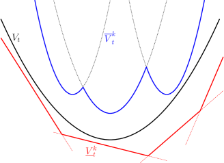
Figure 1: The lower approximations $\underline{V}_{t}^{k}$ will be built as a supremum of basic functions (here affine functions) that will always be below $V_{t}$. Likewise, the upper approximations $\overline{V}_{t}^{k}$ will be built as an infimum of some other basic functions (here quadratic functions) that will always be above $V_{t}$.

2 Notations and definitions

In the sequel, we will use the following notations

$\bullet$ $\mathbb{X}:=\mathbb{R}^{n}$, endowed with its euclidean structure and its Borel $\sigma$-algebra denotes the set of states.

$\bullet$ $T$, a finite integer that we will call the time horizon.

$\bullet$ $\mathop{\mathrm{opt}}$, denotes a generic operation that is either the pointwise infimum or the pointwise supremum of functions which we will call the pointwise optimum.

$\bullet$ $\overline{\mathbb{R}}$, denotes the extended real line endowed with the operations $+\infty+(-\infty)=-\infty+\infty=+\infty$.

$\bullet$ $\mathop{\mathrm{dom}}{\phi}$, denotes the domain of $\phi\in\left(\overline{\mathbb{R}}\right)^{\mathbb{X}}$ defined as the subset of $\mathbb{X}$ in which $\phi(x)\in\mathbb{R}$.

$\bullet$ $\mathbf{F}_{t}$ and $\mathbb{F}_{t}$, denote for every $t\in[\![0,T]\!]$, two subsets of the set $\left(\overline{\mathbb{R}}\right)^{\mathbb{X}}$ such that $\mathbf{F}_{t}\subset\mathbb{F}_{t}$.

$\bullet$ $\phi$ is said to be a basic function if it is an element of $\mathbf{F}_{t}$ for some $t\in[\![0,T]\!]$.

$\bullet$ $\mathbb{\delta}_{X}$ denotes, for every set $X\subset\mathbb{X}$, the function equal to $0$ on $X$ and $+\infty$ elsewhere.

$\bullet$ For every $t\in[\![0,T]\!]$ and every set of basic functions $F_{t}\subset\mathbf{F}_{t}$, we denote by $\mathcal{V}_{F_{t}}$ its pointwise optimum, $\mathcal{V}_{F_{t}}:=\mathop{\mathrm{opt}}_{\phi\in F_{t}}\phi$, that is

$$\begin{array}[]{ccll}\mathcal{V}_{F_{t}}:&\mathbb{X}&\longrightarrow&\overline{\mathbb{R}}\\ &x&\longmapsto&\mathop{\mathrm{opt}}\left\{\phi(x)\mid\phi\in F_{t}\right\}.\end{array}$$ (4)

$\bullet$ $\left(\mathcal{B}_{t}\right)_{t\in[\![0,T-1]\!]}$ denotes a sequence of $T$ operators from $\overline{\mathbb{R}}^{\mathbb{X}}$ to $\overline{\mathbb{R}}^{\mathbb{X}}$, called the Bellman operators.

$\bullet$ $\left(V_{t}\right)_{t\in[\![0,T]\!]}$, denotes, for a fixed function $\psi:\mathbb{X}\to\overline{\mathbb{R}}$, a sequence of value functions given by the system of Bellman Equations (3).

Now, we make several assumptions on the structure of Problem (3). These assumptions will be satisfied in the examples developed in Sections 4 to 6. These assumptions will make it possible to propagate backward in time, regularity of the value function at the final time $t=T$ to the value function at the initial time $t=0$.

Assumption 1 (Structural assumptions)

• Stability by pointwise optimum: for every $t\in[\![0,T]\!]$, if $F_{t}\subset\mathbf{F}_{t}$ then $\mathcal{V}_{F_{t}}\in\mathbb{F}_{t}$.

• Stability by pointwise convergence: for every $t\in[\![0,T]\!]$ if a sequence of functions $(\phi^{k})_{k\in\mathbb{N}}\subset\mathbb{F}_{t}$ converges pointwise to $\phi$ on the domain of $V_{t}$, then $\phi\in\mathbb{F}_{t}$.

• Common regularity: for every $t\in[\![0,T]\!]$, there exists a common (local) modulus of continuity of all $\phi\in\mathbb{F}_{t}$, i.e. for every $x\in\mathop{\mathrm{dom}}(V_{t})$, there exist $\omega_{t,x}:\mathbb{R}_{+}\to\mathbb{R}_{+}\cup\{+\infty\}$ which is increasing, equal to $0$ in $0$, continuous at $0$ and such that for every $\phi\in\mathbb{F}_{t}$ and for every $x^{\prime}\in\mathop{\mathrm{dom}}(V_{t})$, we have that $\lvert\phi(x)-\phi(x^{\prime})\rvert\leq\omega_{t,x}(\lVert x-x^{\prime}\rVert)$.

• Final condition: the value function $V_{T}$ at time $T$ is a pointwise optimum for some given subset $F_{T}$ of $\mathbf{F}_{T}$, that is $\psi:=\mathcal{V}_{F_{T}}$.

• Stability by the Bellman operators: for every $t\in[\![0,T-1]\!]$, if $\phi\in\mathbb{F}_{t+1}$, then $\mathcal{B}_{t}\left(\phi\right)$ belongs to $\mathbb{F}_{t}$.

• Order preserving operators: for every $t\in[\![0,T-1]\!]$, the operators $\mathcal{B}_{t}$ are order preserving, i.e. if $\phi,\varphi\in\mathbb{F}_{t+1}$ are such that $\phi\leq\varphi$, then $\mathcal{B}_{t}\left(\phi\right)\leq\mathcal{B}_{t}\left(\varphi\right)$.

• Additively subhomogeneous operators: for every time step $t\in[\![0,T-1]\!]$, and every given compact set $K_{t}$, there exists $M_{t}>0$ such that the operator $\mathcal{B}_{t}$ restricted to $K_{t}$ is additively subhomogeneous over $\mathbb{F}_{t+1}$, meaning that for every constant function $\lambda\geq 0$ and every function $\phi\in\mathbb{F}_{t+1}$, we have

  $$\mathcal{B}_{t}\left(\phi+\lambda\right)+\mathbb{\delta}_{K_{t}}\leq\mathcal{B}_{t}\left(\phi\right)+\lambda M_{t}+\mathbb{\delta}_{K_{t}}.$$

• Proper value functions: the solution $\left(V_{t}\right)_{t\in[\![0,T]\!]}$ to the Bellman equations (3) never takes the value $-\infty$ and is not identically equal to $+\infty$.

• Compactness condition: for every $t\in[\![0,T-1]\!]$ and every compact set $K_{t}\subset\mathop{\mathrm{dom}}(V_{t})$, there exists a compact set $K_{t+1}\subset\mathop{\mathrm{dom}}(V_{t+1})$ such that, for every function $\phi\in\mathbb{F}_{t+1}$ and constant $\lambda\geq 0$, we have

  $$\mathcal{B}_{t}\left(\phi+\lambda+\mathbb{\delta}_{K_{t+1}}\right)\leq\mathcal{B}_{t}\left(\phi+\lambda\right)+\mathbb{\delta}_{K_{t}}.$$

Remark 1

Assumption 1-(c) ensures that the domain of each function of $\mathbb{F}_{t}$ includes the domain of $V_{t}$. Note that if $\mathbb{F}_{t}$ is the set of all functions satisfying Assumption 1-(c), then Assumption 1-(b) is trivially satisfied. Also note that the domain of $V_{t}$ is known as in [6].

Remark 2

Note that Assumption 1-(h) and 1-(i) do not change whether $\mathop{\mathrm{opt}}=\inf$ or $\mathop{\mathrm{opt}}=\sup$ as the optimal control problem that we consider is formulated as a minimization problem.

Lemma 3

For every $t\in[\![0,T]\!]$ we have that $V_{t}\in\mathbb{F}_{t}$.

Proof. By Assumption 1-(d) and Assumption 1-(a), $V_{T}$ is in $\mathbb{F}_{T}$. Now, assume that for some $t\in[\![0,T-1]\!]$ we have that $V_{t+1}\in\mathbb{F}_{t+1}$. By Assumption 1-(e), we have that $V_{t}=\mathcal{B}_{t}(V_{t+1})\in\mathbb{F}_{t}$ which ends the proof by backward induction. $\Box$

From a set of basic functions $F_{t}\subset\mathbf{F}_{t}$, one can build its pointwise optimum $\mathcal{V}_{F_{t}}=\mathop{\mathrm{opt}}_{\phi\in F_{t}}\phi$. We build a monotone sequence of approximations of the value functions as optima of basic functions which will be computed through compatible selection functions as defined below. We illustrate this definition in Figure 2.

Definition 4 (Compatible selection function)

Let a time step $t\in[\![0,T-1]\!]$ be fixed. A compatible selection function, or simply selection function, is a function $\mathcal{S}_{t}$ from $2^{\mathbf{F}_{t+1}}\times\mathbb{X}$ to $\mathbf{F}_{t}$ satisfying the two following properties

– Validity: for every set of basic functions $F_{t+1}\subset\mathbf{F}_{t+1}$ and every $x\in\mathbb{X}$, we have $\mathcal{S}_{t}\left[F_{t+1},x\right]\leq\mathcal{B}_{t}\left(\mathcal{V}_{F_{t+1}}\right)$ (resp. $\mathcal{S}_{t}\left[F_{t+1},x\right]\geq\mathcal{B}_{t}\left(\mathcal{V}_{F_{t+1}}\right)$) when $\mathop{\mathrm{opt}}=\sup$ (resp. $\mathop{\mathrm{opt}}=\inf$).

– Tightness: for every set of basic functions $F_{t+1}\subset\mathbf{F}_{t+1}$ and every $x\in\mathbb{X}$ the functions $\mathcal{S}_{t}\left[F_{t+1},x\right]$ and $\mathcal{B}_{t}\left(\mathcal{V}_{F_{t+1}}\right)$ coincide at point $x$, that is $\mathcal{S}_{t}\left[F_{t+1},x\right]\left(x\right)=\mathcal{B}_{t}\left(\mathcal{V}_{F_{t+1}}\right)(x).$

For $t=T$, we say that $\mathcal{S}_{T}:2^{\mathbf{F}_{T}}\times\mathbb{X}\to\mathbf{F}_{T}$ is a compatible selection function if it is valid and tight. There, $\mathcal{S}_{T}$ is valid if, for every $F_{T}\subset\mathbf{F}_{T}$ and $x\in\mathbb{X}$, the function $\mathcal{S}_{T}\left(F_{T},x\right)$ remains below (resp. above) the value function at time $T$ when $\mathop{\mathrm{opt}}=\sup$ (resp. $\mathop{\mathrm{opt}}=\inf$). Moreover, the function $\mathcal{S}_{T}$ is tight if it coincides with the value function at point $x$, that is for every $F_{T}\subset\mathbf{F}_{T}$ and $x\in\mathbb{X}$, we have $\mathcal{S}_{T}\left[F_{T},x\right]\left(x\right)=V_{T}(x).$

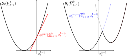
Figure 2: In Sections 4 and 5, we will specify two selection functions, $\phi_{t}^{\text{\tiny SDDP}}$ and $\phi_{t}^{\text{\tiny min-plus}}$, respectively, that will respectively yield upper and lower approximations of the value functions. In both cases, the selection function computes a basic function (in red or blue) which is equal, at the point $x_{t}^{k-1}$, to the image by the Bellman operator of the current approximation (in black), that is the tightness assumption. Moreover it remains above (or below) the image by the Bellman operator of the current approximation, that is the validity assumption.

Note that the Tightness assumption only asks for equality at the point $x$ between the functions $\phi_{t}^{\sharp}\left(F_{t+1},x\right)$ and $\mathcal{B}_{t}\left(\mathcal{V}_{F_{t+1}}\right)$ and not necessarily everywhere. The only global property between the functions $\phi_{t}^{\sharp}\left(F_{t+1},x\right)$ and $\mathcal{B}_{t}\left(\mathcal{V}_{F_{t+1}}\right)$ is an inequality given by the validity assumption.

In Algorithm 1 we will generate, for every time $t$, a sequence of random points of crucial importance that we will call trial points. They will be the ones where the selection functions will be evaluated, given the set $F_{t}^{k}$ which characterizes the current approximation. In order to generate those points, we will assume that we have at our disposition an Oracle which, given $T{+}1$ sets of functions (characterizing the current approximations), computes $T{+}1$ compact sets and a probability law.

Definition 5 (Oracle)

The Oracle takes as input $T{+}1$ sets of functions $F=(F_{0},\ldots,F_{T})$ included in $\mathbf{F}_{0},\ldots,\mathbf{F}_{T}$ respectively. Its output consists of $T{+}1$ compact sets $K_{0},\ldots,K_{T}$, each included in $\mathbb{X}$, and of a probability measure ${\mathbb{P}}_{F}$ on the space $\mathbb{X}^{T+1}$ which are such that

– Initialization. For every $t\in[\![0,T]\!]$, set $F_{t}=\emptyset$ and return $T{+}1$ given compact sets and a given probability measure.

– For every $t\in[\![0,T]\!]$, $K_{t}\subset\mathop{\mathrm{dom}}\left(V_{t}\right)$.

– The support of ${\mathbb{P}}_{F}$ is $K_{0}\times\ldots\times K_{T}$.

For every time $t\in[\![0,T]\!]$, we construct a sequence of functions $\left(V_{t}^{k}\right)_{k\in\mathbb{N}}$ belonging to $\mathbb{F}_{t}$ as follows. For every time $t\in[\![0,T]\!]$ and for every $k\geq 0$, we build a subset $F_{t}^{k}$ of the set $\mathbf{F}_{t}$ and define the sequence of functions by pointwise optimum

$$V_{t}^{k}:=\mathcal{V}_{F_{t}^{k}}=\mathop{\mathrm{opt}}_{\phi\in F_{t}^{k}}\phi\;.$$ (5)

As described here, the functions are just byproducts of Algorithm 1, which only describes the way the sets $F_{t}^{k}$ are computed.

As the following algorithm was inspired by Qu’s work which uses tropical algebra techniques, we will call this algorithm “Tropical Dynamic Programming”.

Algorithm 1 Tropical Dynamic Programming (TDP)

0:  For every $t\in[\![0,T]\!]$, $\mathcal{S}_{t}$ a compatible selection function and a Trial point Oracle satisfying Definition 5.

0:  For every $t\in[\![0,T]\!]$, a sequence of sets $\left(F_{t}^{k}\right)_{k\in\mathbb{N}}$ and the associated sequence $V_{t}^{k}=\mathop{\mathrm{opt}}_{\phi\in F_{t}^{k}}\phi$.

  Define for every $t\in[\![0,T]\!]$, $F_{t}^{0}:=\emptyset$.

  for $k\geq 0$ do

     Forward phase

     Compute $\left(K_{0}^{k},\dots K_{T}^{k},\mathbb{P}^{k}\right)=\text{Oracle}\left(F^{k}_{0},\dots,F^{k}_{T}\right).$

     Draw trial points $\left(x_{t}^{k}\right)_{t\in[\![0,T]\!]}$ over $K_{0}^{k}\times K_{1}^{k}\times\ldots\times K_{T}^{k}$ according to $\mathbb{P}^{k}$ knowing the past iterations.

     Backward phase

     Compute $\phi_{T}^{k+1}:=\mathcal{S}_{T}\left[F^{k}_{T},x_{T}^{k}\right]$.

     Define $F_{T}^{k+1}:=F_{T}^{k}\cup\left\{\phi_{T}^{k+1}\right\}$.

     for $t$ from $T-1$ to $0$ do

        Compute $\phi_{t}^{k+1}:=\mathcal{S}_{t}\left[F^{k+1}_{t+1},x_{t}^{k}\right]$.

        Define $F_{t}^{k+1}:=F_{t}^{k}\cup\left\{\phi_{t}^{k+1}\right\}$.

     end for

  end for

At each iteration, Algorithm 1 generates a trial point $x_{t}^{k}$ which only depends on the data available at the current iteration. We loosely explain this point. Define for every $k\in\mathbb{N}$, $F^{k}=(F_{t}^{k})_{t\in[\![0,T]\!]}$ and $x^{k}=(x_{t}^{k})_{t\in[\![0,T]\!]}$. Then, there exists a deterministic function $\xi$ and a sequence of independent random variables $(W^{k})_{k\in\mathbb{N}}$ such that for every $k\in\mathbb{N}$, $x^{k}=\xi(F^{k},W^{k})$ where $(W^{k})_{k\in\mathbb{N}}$ is furthermore independent from $F^{0}$. Throughout the remainder of the article, denote by $(\Omega,\mathcal{F},\mathbb{P})$ a probability space on which the random variables $(W^{k})_{k\in\mathbb{N}}$ are defined and independent.

We will denote by $+$ the Minkowski sum between sets, by $\mathbb{B}$ the unit closed euclidean ball of $\mathbb{X}^{T+1}$ and for every $x\in\mathbb{X}^{T+1}$ and radius $r>0$, $B(x,r)$ is the euclidean open ball of radius $r$ centered at $x$. Furthermore, we define for every $t$, $K_{t}^{*}:=\limsup_{k\in\mathbb{N}}K_{t}^{k}$ the set of all possible limit points of $K_{t}^{k}$. We make the following assumption on the Oracle which, loosely stated, ensures that if a state $x_{t}$ is close to $K_{t}^{*}$, then $x_{t}$ is almost a limit point of the sequence of trial points $(x_{t}^{k})_{k\in\mathbb{N}}$.

Assumption 2 (Trial point assumption)

For every radius $r^{\prime}>0$, there exists $r>0$ such that

$$\forall x\in\mathbb{X}\;,\enspace\mathbb{P}\Big{[}\big{(}x\in\limsup_{k\in\mathbb{N}}K^{k}+r\mathbb{B}\big{)}\Rightarrow x\in\limsup_{k\in\mathbb{N}}B(x^{k},r^{\prime})\Big{]}=1\;.$$ (6)

Remark that $(\limsup_{k\in\mathbb{N}}K^{k})+r\mathbb{B}=\limsup_{k\in\mathbb{N}}(K^{k}+r\mathbb{B})$, hence the lack of parenthesis. The following lemma gives some more insight on the Trial point assumption.

Lemma 6

Consider the sequence of trial points $(x^{k})_{k\in\mathbb{N}}$ generated by Algorithm 1 with an Oracle satisfying Assumption 2. Given $r^{\prime}>0$ and $x\in\mathbb{X}$, for every $r^{\prime\prime}>r^{\prime}$, $\mathbb{P}$-a.s.,

$$x\in\limsup_{k\in\mathbb{N}}B(x^{k},r^{\prime})\Rightarrow x^{k}\in B(x,r^{\prime\prime})\ \text{for infinitely many indices}\ k\in\mathbb{N}\;.$$ (7)

Conversely, given $r^{\prime\prime}>0$ and $x\in\mathbb{X}$, for every $r^{\prime}>r^{\prime\prime}$, $\mathbb{P}$-a.s.

$$x^{k}\in B(x,r^{\prime\prime})\ \text{for infinitely many indices}\ k\in\mathbb{N}\Rightarrow x\in\limsup_{k\in\mathbb{N}}B(x^{k},r^{\prime})\;.$$ (8)

Proof. First, we prove Equation (7). Fix $r^{\prime\prime}>r^{\prime}>0$ and assume that $x\in\limsup_{k\in\mathbb{N}}B(x^{k},r^{\prime})$, $\mathbb{P}$-a.s.. Then, there exists an increasing function $\sigma:\mathbb{N}\to\mathbb{N}$ and a sequence $(y^{\sigma(k)})_{k\in\mathbb{N}}\subset r^{\prime}\mathbb{B}$ such that $x^{\sigma(k)}+y^{\sigma(k)}\underset{k\to+\infty}{\longrightarrow}x$. As $r^{\prime\prime}-r^{\prime}>0$, there exists a rank $k_{0}\in\mathbb{N}$ such that when $k\geq k_{0}$ we have $\lVert x-x^{\sigma(k)}+y^{\sigma(k)}\rVert\leq r^{\prime\prime}-r^{\prime}$. By triangle inequality, we have

$$\lVert x-x^{\sigma(k)}\rVert\leq\lVert x-x^{\sigma(k)}+y^{\sigma(k)}\rVert+\lVert-y^{\sigma(k)}\rVert\\ \leq(r^{\prime\prime}-r^{\prime})+r^{\prime}=r^{\prime\prime},$$

i.e. $\mathbb{P}$-a.s., for every $k\geq k_{0}$, $x\in B(x^{k},r^{\prime\prime})$, which yields Equation (7).

Second, we prove Equation (8). Fix $r^{\prime}>r^{\prime\prime}>0$ and assume that $x^{k}\in B(x,r^{\prime\prime})$ for infinitely many indices $k\in\mathbb{N}$. Thus, $\mathbb{P}$-a.s, there exists an increasing function $\sigma:\mathbb{N}\to\mathbb{N}$ and a sequence $(y^{\sigma(k)})_{k\in\mathbb{N}}\subset r^{\prime\prime}\mathbb{B}$ such that $x^{\sigma(k)}-x=y^{\sigma(k)}$. As $r^{\prime}>r^{\prime\prime}$, $\mathbb{P}$-a.s. $x\in B(x^{k},r^{\prime})$ and $x=x^{\sigma(k)}-y^{\sigma(k)}.$ Hence, we obtain Equation (8). $\Box$

Now, we give two examples of Oracles that satisfy the Trial point assumption 2. They are used respectively in Section 4 and 5.

Example 1 (Independant uniform draws over the unit sphere)

Consider the Oracle which constantly outputs $T+1$ times the unit euclidean sphere $\mathbf{S}$ of $\mathbb{X}$ and the uniform probability measure $\mathbb{P}^{k}:=\sigma_{U}$ of $\mathbf{S}^{T+1}$ on $\mathbb{X}^{T+1}$. Here, we have for every $k\in\mathbb{N}$, $K^{k}=\mathbf{S}^{T+1}$. Fix an arbitrary $r^{\prime}>0$ and set $r=r^{\prime}/2$, we prove that

$$\forall x\in\mathbb{X},{\mathbb{P}}\Big{[}x\in(\mathbf{S}^{T+1}+r\mathbb{B})\Rightarrow x\in\limsup_{k\in\mathbb{N}}B(x^{k},r^{\prime})\Big{]}=1\;.$$

Proof. Fix $x\in\mathbf{S}^{T+1}+r\mathbb{B}$, we need to show that we have $\mathbb{P}\big{[}x\in\limsup_{k\in\mathbb{N}}B(x^{k},r^{\prime})\big{]}=1$. Now, fix $r^{\prime\prime}>0$ such that $r<r^{\prime\prime}<r^{\prime}$. Using Lemma 6-(8), it is enough to show that

$$\mathbb{P}[x^{k}\in B(x,r^{\prime\prime})\ \text{for infinitely many indices}\ k\in\mathbb{N}]=1.$$ (9)

As $r^{\prime\prime}>r$ and $x$ is distant from $\mathbf{S}^{T+1}$ by less than $r$, the quantity $\mathbb{P}[x^{k}\in B(x,r^{\prime\prime})]=\sigma_{U}[B(x,r^{\prime\prime})\cap\mathbf{S}^{T+1}]$ is a positive constant in $k$. Thus, we have that $\sum_{k\in\mathbb{N}}\mathbb{P}\big{[}x^{k}\in B(x,r^{\prime\prime})\big{]}=+\infty$. Moreover, the sequence of events $(x^{k}\in B(x,r))_{k\in\mathbb{N}}$ are independent, thus by Borel-Cantelli’s Lemma, Equation (9) holds. $\Box$

Example 2 (Dirac on the current optimal trajectory)

The sequence of Probability measures $({\mathbb{P}}^{k})_{k\in\mathbb{N}}$ is recursively build as follows:

– Set ${\mathbb{P}}^{0}:=(\delta_{x_{0}^{0}},\ldots\delta_{x_{T}^{0}})$ where $x_{t}^{0}\in K_{t}^{0}$ for every $t\in[\![0,T]\!]$.

– Given sets of functions $F_{0}^{k},\ldots,F_{T}^{k}$. Start, by fixing $x_{0}^{k}=x_{0}$ and compute forward in time, for $t\in[\![0,T{-}1]\!]$, optimal controls by $u_{t}^{k}\in\mathop{\arg\min}_{u}\mathcal{B}_{t}^{u}(\mathcal{V}_{F_{t+1}^{k}})(x_{t}^{k}),$ and successive states by $x_{t+1}^{k}=f_{t}(x_{t}^{k},u_{t}^{k})$.

– Define a probability measures ${\mathbb{P}}^{k}:=(\delta_{x^{k}_{0}},\ldots,\delta_{x^{k}_{T}})$.

Consider the Oracle which, given sets of functions $F_{0}^{k},\ldots,F_{T}^{k}$, outputs the singleton $\left\{x^{k}\right\}=\big{\{}(x^{k}_{t})_{t\in[\![0,T]\!]}\big{\}}$ and the probability measure ${\mathbb{P}}^{k}:=(\delta_{x^{k}})$ defined at previous step. Fix $r>0$, take $r^{\prime}=r>0$ and $x\in\mathbb{X}^{T+1}$. We obtain that

$${\mathbb{P}}\Big{[}x\in\big{(}\limsup_{k\in\mathbb{N}}\underbrace{\{x^{k}\}+r\mathbb{B}}_{=B(x^{k},r)}\big{)}^{c}\ \text{or}\ x\in\limsup_{k\in\mathbb{N}}B(x^{k},r)\Big{]}=1\;,$$

which is equivalent to the Trial point assumption with $K^{k}=\{x^{k}\}$.

3 Almost sure convergence on the set of accumulation points

In this section, we will prove the convergence result stated in Theorem 13. For this purpose, we state several crucial properties of the approximation functions $\left(V_{t}^{k}\right)_{k\in\mathbb{N}}$ generated by Algorithm 1. They are direct consequences of the facts that the Bellman operators are order preserving and that the basic functions building our approximations are computed through compatible selection functions. The Algorithm 1 is stochastic, as trial points are drawn at each iteration from $\mathbb{P}^{k}$. Therefore, equalities, inequalities and statements where the functions $V_{t}^{k}$ are involved hold $\mathbb{P}$-almost surely. However, for the sake of simplicity, we will refrain from always adding $\mathbb{P}$-almost surely in equalities, inequalities and some statements.

Lemma 7

The sequence of functions $\left(V_{t}^{k}\right)_{k\in\mathbb{N}}$, for every $t\in[\![0,T]\!]$, given by Equation (5) and produced by Algorithm 1 satisfy the following properties.

1. Monotone approximations: for every indices $k<k^{\prime}$ and every $t\in[\![0,T]\!]$, we have that $V_{t}^{k}\geq V_{t}^{k^{\prime}}\geq V_{t}$ when $\mathop{\mathrm{opt}}=\inf$ and $V_{t}^{k}\leq V_{t}^{k^{\prime}}\leq V_{t}$ when $\mathop{\mathrm{opt}}=\sup$.

2. For every $k\in\mathbb{N}$ and every $t\in[\![0,T-1]\!]$, we have that $\mathcal{B}_{t}\left(V_{t+1}^{k}\right)\leq V_{t}^{k}$ when $\mathop{\mathrm{opt}}=\inf$ and $\mathcal{B}_{t}\left(V_{t+1}^{k}\right)\geq V_{t}^{k}$ when $\mathop{\mathrm{opt}}=\sup$.

3. For every $k\geq 1$ and every $t\in[\![0,T-1]\!]$, we have $\mathcal{B}_{t}\left(V_{t+1}^{k}\right)\left(x_{t}^{k-1}\right)=V_{t}^{k}\left(x_{t}^{k-1}\right)$.

4. For every $k\geq 1$, we have $V_{T}^{k}\left(x_{T}^{k-1}\right)=V_{T}\left(x_{T}^{k-1}\right)$.

Proof. We prove each point when $\mathop{\mathrm{opt}}=\inf$. The case $\mathop{\mathrm{opt}}=\sup$ is similar and left to the reader.

$\bullet$ (1) (left inequality). Let $t\in[\![0,T]\!]$ be fixed. By construction of Algorithm 1, the sequence of sets $\big{(}F_{t}^{k}\big{)}_{k\in\mathbb{N}}$ is non-decreasing. Now, using the definition of the sequence $\left(V_{t}^{k}\right)_{k\in\mathbb{N}}$ given by Equation (5) we have that $V_{t}^{k+1}=\mathcal{V}_{F^{k+1}_{t}}(x)=\inf_{\phi\in F^{k+1}_{t}}\phi(x)\leq\inf_{\phi\in F^{k}_{t}}\phi(x)=\mathcal{V}_{F^{k}_{t}}(x)=V_{t}^{k}$ and thus the sequence $\left(V_{t}^{k}\right)_{k\in\mathbb{N}}$ is non-increasing.

$\bullet$ (2). We prove the assertion by induction on $k\in\mathbb{N}$. For $k=0$, as $F_{t}^{0}=\emptyset$, we have $V_{t}^{0}=+\infty$ for all $t\in[\![0,T-1]\!]$ and thus the assertion is true. Now, assume that for some $k\in\mathbb{N}$, we have for all $t\in[\![0,T-1]\!]$

$$\mathcal{B}_{t}\left(V_{t+1}^{k}\right)\leq V_{t}^{k}\;.$$ (10)

Since $\big{(}V_{t+1}^{k^{\prime}}\big{)}_{k^{\prime}\in\mathbb{N}}$ is non-increasing by already proved Item (1) and $\mathcal{B}_{t}$ is order preserving using Assumption 1-(f), we have that $\mathcal{B}_{t}\left(V_{t+1}^{k+1}\right)\leq\mathcal{B}_{t}(V_{t+1}^{k})$. This last inequality combined with induction assumption given by Equation (10) gives the inequality

$$\mathcal{B}_{t}\left(V_{t+1}^{k+1}\right)\leq V_{t}^{k}\;.$$ (11)

Moreover, we also have that

$$\mathcal{B}_{t}\left(V_{t+1}^{k+1}\right) \mathop{=}_{(\text{by }~{}\eqref{Vktdef})}\mathcal{B}_{t}\left(\mathcal{V}_{F_{t+1}^{k+1}}\right)\mathop{\leq}_{(\text{by }\mathcal{S}_{t}\text{ validity at }x_{t}^{k})}\mathcal{S}_{t}\left[F_{t+1}^{k+1},x^{k}_{t}\right]=\phi^{k+1}_{t}\;,$$ (12)

where the last equality is obtained by definition of function $\phi^{k+1}_{t}$ in Algorithm 1. Thus, combining Equation (11) and (12) we have that $\mathcal{B}_{t}(V_{t+1}^{k+1})\leq\inf\big{(}V_{t}^{k},\phi_{t}^{k+1}\big{)}$. Finally, using Equation (5) and Algorithm 1, we have that

$$\inf\big{(}V_{t}^{k},\phi_{t}^{k+1}\big{)}=\inf\Big{(}\inf_{\phi\in F_{t}^{k}}\phi,\phi_{t}^{k+1}\Big{)}=\inf_{\phi\in F_{t}^{k}\cup\{\phi_{t}^{k+1}\}}\phi=\inf_{\phi\in F_{t}^{k+1}}\phi=V_{t}^{k+1}\;.$$

Thus, we obtain that $\mathcal{B}_{t}\left(V_{t+1}^{k+1}\right)\leq\inf\big{(}V_{t}^{k},\phi_{t}^{k+1}\big{)}=V_{t}^{k+1}$, which gives the induction assumption for $k+1$ and concludes the proof of (2).

$\bullet$ (3). As the selection function $\mathcal{S}_{t}$ is tight in the sense of Definition 4, we have by construction of Algorithm 1 that $\mathcal{B}_{t}(V_{t+1}^{k})(x_{t}^{k-1})=\phi_{t}^{k}(x_{t}^{k-1})$. Combining this equation with Item (2) and the definition of $V_{t}^{k}$, one gets Lemma 7-(3).

$\bullet$ (4). Similarly, we have that $V_{T}(x_{T}^{k-1})=\phi_{T}^{k}(x_{T}^{k-1})$, which combined with the inequality given in Item (1) and the definition of $V_{T}^{k}$ gives Lemma 7-(4).

$\bullet$ (1) (right inequality). We prove that $V_{t}^{k}\geq V_{t}$ for all for all $k\in\mathbb{N}$ and all $t\in[\![0,T]\!]$. Fix $k\in\mathbb{N}$, we show that $V_{t}^{k}\geq V_{t}$ for all $t\in[\![0,T]\!]$ by backward recursion on time $t$. For $t=T$, by validity of the selection functions given in Definition 4, for every $\phi\in F_{T}^{k}$, we have that $\phi\geq V_{T}$. Thus $V_{T}^{k}=\mathcal{V}_{F_{T}^{k}}=\inf_{\phi\in F_{T}^{k}}\phi\geq V_{T}$. Now, suppose that for some $t\in[\![0,T-1]\!]$, we have that $V_{t+1}\leq V_{t+1}^{k}$. Then, using the definition of the value function in Equation (3), the fact that the Bellman operators are order preserving and the inequality already proved in Item (2) we obtain that: $V_{t}=\mathcal{B}_{t}\big{(}V_{t+1}\big{)}\leq\mathcal{B}_{t}\big{(}V_{t+1}^{k}\big{)}\leq V_{t}^{k}\;,$ which gives the assertion for time $t$. This ends the proof. $\Box$

In the following two propositions, we state that the sequences $\left(V_{t}^{k}\right)_{k\in\mathbb{N}}$ and $(\mathcal{B}_{t}\left(V_{t+1}^{k}\right))_{k\in\mathbb{N}}$ converge uniformly on any compact included in the domain of $V_{t}$. The limit function $V_{t}^{*}$ of $\left(V_{t}^{k}\right)_{k\in\mathbb{N}}$ will be a natural candidate to be equal to the value function $V_{t}$.

Lemma 8

Fix $t\in[\![0,T]\!]$. Let $(\phi^{k})_{k\in\mathbb{N}}$ be a monotonic sequence in $\mathbb{F}_{t}$ such that there exists $\phi_{1},\phi_{2}\in\mathbb{F}_{t}$ satisfying for every $k\in\mathbb{N}$ $\phi_{1}\leq\phi^{k}\leq\phi_{2}.$ Then, the sequence $(\phi^{k})_{k\in\mathbb{N}}$ converges uniformly on every compact set included in $\mathop{\mathrm{dom}}(V_{t})$ to a function $\phi^{*}\in\mathbb{F}_{t}$.

Proof. The proof relies on the Arzela-Ascoli theorem [15, Theorem 2.13.30 p.347]. Since $\phi_{1}$ and $\phi_{2}$ belong to $\mathbb{F}_{t}$, they are finite on $\mathop{\mathrm{dom}}(V_{t})$. Then, the sequence of functions $(\phi^{k})_{k\in\mathbb{N}}$ is monotonic and bounded, so it converges pointwise on $\mathop{\mathrm{dom}}(V_{t})$ to a limit function $\phi^{*}$. By Assumption 1-(b), this implies that $\phi^{*}\in\mathbb{F}_{t}$.

Now, fix a compact set $K\subset\mathop{\mathrm{dom}}(V_{t})$. First, since $(\phi^{k})_{k\in\mathbb{N}}\subset\mathbb{F}_{t}$, we have that for every $k\in\mathbb{N}$, $\mathop{\mathrm{dom}}(\phi^{k})$ contains $\mathop{\mathrm{dom}}(V_{t})$ and the sequence $(\phi^{k})_{k\in\mathbb{N}}$ share a common modulus of continuity. Second, the continuous functions $\lvert\phi_{1}\rvert$ and $\lvert\phi_{2}\rvert$ are bounded from above by quantities independent of $x$ on the compact $K$, thus, $\sup_{k\in\mathbb{N}}\sup_{x\in K}\lvert\phi^{k}(x)\rvert$ is finite. Hence, by Arzela-Ascoli theorem the monotonic sequence $(\phi^{k})_{k\in\mathbb{N}}$ converges uniformly on the compact $K$ to the continuous function $\phi^{*}$. $\Box$

Proposition 9 (Existence of an approximating limit)

Let $t\in[\![0,T]\!]$ be fixed, the sequence of functions $\left(V_{t}^{k}\right)_{k\in\mathbb{N}}$ defined by Equation (5) and Algorithm 1 $\mathbb{P}$-a.s. converges uniformly on every compact set included in the domain of $V_{t}$ (solution of Equation (3)) to a function $V_{t}^{*}\in\mathbb{F}_{t}$.

Proof. By Lemma 7-(1), for every $k\geq 1$ we have that $V_{t}^{1}\leq V_{t}^{k}\leq V_{t}$, when $\mathop{\mathrm{opt}}=\sup$ (and the inequalities are reversed when $\mathop{\mathrm{opt}}=\inf$). Now, we have that $V_{t}^{1}\in\mathbb{F}_{t}$ and by Lemma 3, the mapping $V_{t}$ is also in $\mathbb{F}_{t}$. Moreover, by Lemma 7-(1), the sequence $(V_{t}^{k})_{k\geq 1}$ is monotonic. Thus, by Lemma 8, we have that $(V_{t}^{k})_{k\geq 1}$ converges uniformly on every compact set included in $\mathop{\mathrm{dom}}(V_{t})$ to a function $V_{t}^{*}\in\mathbb{F}_{t}$.

This ends the proof. $\Box$

Proposition 10

Let $t\in[\![0,T-1]\!]$ be fixed and $V_{t+1}^{*}$ be the function defined in Proposition 9. The sequence $\mathcal{B}_{t}\left(V_{t+1}^{k}\right)$ $\mathbb{P}$-a.s. converges uniformly to the continuous function $\mathcal{B}_{t}\left(V_{t+1}^{*}\right)$ on every compact sets included in the domain of $V_{t}$.

Proof. First we consider the case $\mathop{\mathrm{opt}}=\inf$. As the sequence $\left(V_{t+1}^{k}\right)_{k\in\mathbb{N}}$ is non-increasing and using the fact that the operator $\mathcal{B}_{t}$ is order preserving, the sequence $(\mathcal{B}_{t}(V_{t+1}^{k}))_{k\in\mathbb{N}}$ is also non-increasing. Moreover, we have that

$$V_{t}^{1} \geq V_{t}^{k}$$ (Lemma 7-(1))

$$\geq\mathcal{B}_{t}(V_{t+1}^{k})$$ (Lemma 7-(2))

$$\geq\mathcal{B}_{t}(V_{t+1})$$ (Lemma 7-(1))

$$=V_{t}.$$

Thus, by Lemma 8, the sequence of functions $(\mathcal{B}_{t}(V_{t+1}^{k}))_{k\geq 1}$ converges uniformly on every compact set included in $\mathop{\mathrm{dom}}(V_{t})$ to a function $\phi\in\mathbb{F}_{t}$. Let $K_{t}$ be a given compact set included in $\mathop{\mathrm{dom}}(V_{t})$. We now show that the function $\phi$ is equal to $\mathcal{B}_{t}\left(V_{t+1}^{*}\right)$ on the given compact $K_{t}$ or equivalently we show that $\phi+\mathbb{\delta}_{K_{t}}=\mathcal{B}_{t}\left(V_{t+1}^{*}\right)+\mathbb{\delta}_{K_{t}}$. As already shown in Proposition 9, we have that $V_{t+1}^{k}\geq V_{t+1}^{*}$, which combined with the fact that the operator $\mathcal{B}_{t}$ is order preserving, gives, for every $k\geq 1$, that $\mathcal{B}_{t}(V_{t+1}^{k})\geq\mathcal{B}_{t}(V_{t+1}^{*}).$ Now, adding on both side of the previous inequality the mapping $\mathbb{\delta}_{K_{t}}$ and taking the limit as $k$ goes to infinity, we have that

$$\phi+\mathbb{\delta}_{K_{t}}\geq\mathcal{B}_{t}\left(V_{t+1}^{*}\right)+\mathbb{\delta}_{K_{t}}.$$

For the converse inequality, start by recalling that, by the compactness condition (see Assumption 1-(i)), there exists a compact set $K_{t+1}\subset\mathop{\mathrm{dom}}(V_{t+1})$ such that, for every $\phi\in\mathbb{F}_{t+1}$ and every $\lambda\geq 0$, we have that

$$\mathcal{B}_{t}\left(\phi+\lambda+\mathbb{\delta}_{K_{t+1}}\right)\leq\mathcal{B}_{t}\left(\phi+\lambda\right)+\mathbb{\delta}_{K_{t}}.$$ (13)

Now, by Proposition 9, the non-increasing sequence $\left(V_{t+1}^{k}\right)_{k\in\mathbb{N}}$ converges uniformly to $V_{t+1}^{*}\in\mathbb{F}_{t+1}$ on the compact set $K_{t+1}$. Thus, for any fixed $\epsilon>0$, there exists an integer $k_{0}\in\mathbb{N}$, such that we have

$$V_{t+1}^{k}\leq V_{t+1}^{k}+\mathbb{\delta}_{K_{t+1}}\leq V_{t+1}^{*}+\epsilon+\mathbb{\delta}_{K_{t+1}}\,,$$

for all $k\geq k_{0}$. By Assumption 1-(f) and Assumption 1-(g), the operator $\mathcal{B}_{t}$ is order preserving and additively $M_{t}$-subhomogeneous, thus we get using Equation (13) that

$$\mathcal{B}_{t}\left(V_{t+1}^{k}\right)\leq\mathcal{B}_{t}\left(V_{t+1}^{k}+\mathbb{\delta}_{K_{t+1}}\right) \leq\mathcal{B}_{t}(V_{t+1}^{*}+\epsilon+\mathbb{\delta}_{K_{t+1}}),$$ (by Assumption 1-(f))

$$\leq\mathcal{B}_{t}(V_{t+1}^{*}+\epsilon)+\mathbb{\delta}_{K_{t}},$$ (by Equation (13))

$$\leq\mathcal{B}_{t}(V_{t+1}^{*})+M_{t}\epsilon+\mathbb{\delta}_{K_{t}}\;.$$ (by Assumption 1-(g))

Adding $\mathbb{\delta}_{K_{t}}$ on the left hand side, we have for every $k\geq k_{0}$ that $\mathcal{B}_{t}\left(V_{t+1}^{k}\right)+\mathbb{\delta}_{K_{t}}\leq\mathcal{B}_{t}\left(V_{t+1}^{*}\right)+M_{t}\epsilon+\mathbb{\delta}_{K_{t}}.$ Thus, taking the limit when $k$ goes to infinity we obtain that

$$\phi+\mathbb{\delta}_{K_{t}}\leq\mathcal{B}_{t}\left(V_{t+1}^{*}\right)+M_{t}\epsilon+\mathbb{\delta}_{K_{t}}.$$

The result has been proved for all $\epsilon>0$ and we have thus shown that $\phi=\mathcal{B}_{t}\left(V_{t+1}^{*}\right)$ on the compact set $K_{t}$. We conclude that $\left(\mathcal{B}_{t}\left(V_{t+1}^{k}\right)\right)_{k\in\mathbb{N}}$ converges uniformly to the function $\mathcal{B}_{t}\left(V_{t+1}^{*}\right)$ on the compact set $K_{t}$. For the case $\mathop{\mathrm{opt}}=\sup$, mutatis mutantis we have that $\mathcal{B}_{t}(V_{t+1}^{k})\leq\mathcal{B}_{t}(V_{t+1}^{*}).$ Similarly, as the sequence $(V_{t+1}^{k})$ is non-decreasing and $\mathcal{B}_{t}$ is order preserving, one gets that for every $k$ large enough

$$\mathcal{B}_{t}(V_{t+1}^{*})\geq\mathcal{B}_{t}(V_{t+1}^{*})+\mathbb{\delta}_{K_{t+1}}\geq\mathcal{B}_{t}(V_{t+1}^{*}+\epsilon+\mathbb{\delta}_{K_{t+1}}).$$

Thus, by Equation (13) and $M_{t}$-sub-homogeneity we have that $\mathcal{B}_{t}(V_{t+1}^{*})+\mathbb{\delta}_{K_{t}}\leq\mathcal{B}_{t}(V_{t+1}^{k})+M_{t}\epsilon+\mathbb{\delta}_{K_{t}},$ which yields the result when $k$ goes to infinity. This ends the proof. $\Box$

We want to exploit the fact that our approximations of the final cost function are exact in the sense that we have equality between $V_{T}^{k}$ and $V_{T}$ at the points drawn in Algorithm 1, that is, the tightness assumption of the selection function is much stronger at time $T$ than for times $t<T$. Thus we want to propagate the information backward in time: starting from time $t=T$ we want to deduce information on the approximations for times $t<T$.

In order to show that $V_{t}=V_{t}^{*}$ on some set $S_{t}$, a dissymmetry between upper and lower approximations is emphasized. We introduce the notion of optimal sets $\left(S_{t}\right)_{t\in[\![0,T]\!]}$ with respect to a sequence of functions $\left(\phi_{t}\right)_{t\in[\![0,T]\!]}$ as a condition on the sets $\left(S_{t}\right)_{t\in[\![0,T]\!]}$ such that in order to compute the restriction of $\mathcal{B}_{t}\left(\phi_{t+1}\right)$ to $S_{t}$, one only needs to know $\phi_{t+1}$ on the set $S_{t+1}$. The Figure 3 illustrates this notion.

Definition 11 (Optimal sets)

Let $\left(\phi_{t}\right)_{t\in[\![0,T]\!]}$ be $T{+}1$ functions on $\mathbb{X}$. A sequence of sets $\left(S_{t}\right)_{t\in[\![0,T]\!]}$ is said to be $\left(\phi_{t}\right)$-optimal if for every $t\in[\![0,T-1]\!]$, we have

$$\mathcal{B}_{t}\left(\phi_{t+1}+\mathbb{\delta}_{S_{t+1}}\right)+\mathbb{\delta}_{S_{t}}=\mathcal{B}_{t}\left(\phi_{t+1}\right)+\mathbb{\delta}_{S_{t}}.$$ (14)

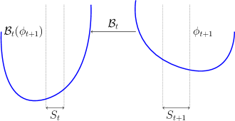
Figure 3: The optimality of the sets $\left(S_{t}\right)_{t\in[\![0,T]\!]}$ means that in order to compute the restriction of $\mathcal{B}_{t}\left(\phi_{t+1}\right)$ on $S_{t}$, one only needs to know the values of $\phi_{t+1}$ on the set $S_{t+1}$.

When approximating from below, the optimality of sets is only needed for the limit functions $\left(V_{t}^{*}\right)_{t\in[\![0,T]\!]}$, whereas when approximating from above, one needs the optimality of sets with respect to the value functions $\left(V_{t}\right)_{t\in[\![0,T]\!]}$. It seems easier to ensure the $(V_{t}^{*})$-optimality of sets than $(V_{t})$-optimality as the function $V_{t}^{*}$ is known through the sequence $\left(V_{t}^{k}\right)_{k\in\mathbb{N}}$, whereas the function $V_{t}$ is, a priori, unknown. This fact is discussed in Sections 4 and 5.

Lemma 12 (Uniqueness in restricted Bellman Equations)

Let $\left(X_{t}\right)_{t\in[\![0,T]\!]}$ be a sequence of sets such that for every $t\in[\![0,T]\!]$, $X_{t}\subset\mathop{\mathrm{dom}}(V_{t})$ and which is

– $(V_{t})$-optimal when $\mathop{\mathrm{opt}}=\inf$,

– $(V_{t}^{*})$-optimal when $\mathop{\mathrm{opt}}=\sup$.

If the sequence of functions $\left(V_{t}^{*}\right)_{t\in[\![0,T]\!]}$ satisfies the following restricted Bellman Equations:

$$V_{T}^{*}+\delta_{X_{T}}=\psi+\delta_{X_{T}}\quad\text{ and }\quad\forall t\in[\![0,T-1]\!],\ \mathcal{B}_{t}\left(V_{t+1}^{*}\right)+\mathbb{\delta}_{X_{t}}=V_{t}^{*}+\mathbb{\delta}_{X_{t}}\;.$$ (15)

Then, for every $t\in[\![0,T]\!]$ and every $x\in X_{t}$, we have that $V_{t}^{*}(x)=V_{t}(x)$.

Proof. We prove the lemma by backward induction on time $t\in[\![0,T]\!]$. We first treat the case $\mathop{\mathrm{opt}}=\inf$. At time $t=T$, since $V_{T}$ is given by Equation (3), we have $V_{T}=\psi$. We therefore have by Equation (15) that $V_{T}^{*}+\mathbb{\delta}_{X_{T}}=\psi+\mathbb{\delta}_{X_{T}}=V_{T}+\mathbb{\delta}_{X_{T}}$, which gives the fact that functions $V_{T}^{*}$ and $V_{T}$ coincide on the set $X_{T}$. Now, let time $t\in[\![0,T-1]\!]$ be fixed and assume that we have $V_{t+1}^{*}(x)=V_{t+1}(x)$ for every $x\in X_{t+1}$, or equivalently:

$$V_{t+1}^{*}+\mathbb{\delta}_{X_{t+1}}=V_{t+1}+\mathbb{\delta}_{X_{t+1}}\,.$$ (16)

Using Lemma 7-(1), the sequence of functions $(V_{t}^{k})_{k\in\mathbb{N}}$ is lower bounded by $V_{t}$. Taking the limit in $k$, we obtain that $V_{t}^{*}\geq V_{t}$, thus we only have to prove that $V_{t}^{*}\leq V_{t}$ on $X_{t}$, that is $V_{t}^{*}+\mathbb{\delta}_{X_{t}}\leq V_{t}+\mathbb{\delta}_{X_{t}}$. We successively have:

$$V_{t}^{*}+\mathbb{\delta}_{X_{t}} =\mathcal{B}_{t}\left(V_{t+1}^{*}\right)+\mathbb{\delta}_{X_{t}}$$ (by (15))

$$\leq\mathcal{B}_{t}\left(V_{t+1}^{*}+\mathbb{\delta}_{X_{t+1}}\right)+\mathbb{\delta}_{X_{t}} \mathcal{B}_{t}$$ ( is order preserving)

$$=\mathcal{B}_{t}\left(V_{t+1}+\mathbb{\delta}_{X_{t+1}}\right)+\mathbb{\delta}_{X_{t}}$$ (by induction assumption (16))

$$=\mathcal{B}_{t}\left(V_{t+1}\right)+\mathbb{\delta}_{X_{t}} (X_{t})_{{t\in[\![0,T]\!]}} (V_{t})$$ (by (14), is -optimal)

$$=V_{t}+\mathbb{\delta}_{X_{t}},$$ (by (3))

which concludes the proof in the case of $\mathop{\mathrm{opt}}=\inf$.

Now we prove the case $\mathop{\mathrm{opt}}=\sup$ in a similar way by backward induction on time $t\in[\![0,T]\!]$. As for the case $\mathop{\mathrm{opt}}=\inf$, at time $t=T$, one has $V_{T}^{*}+\mathbb{\delta}_{X_{T}}=V_{T}+\mathbb{\delta}_{X_{T}}$. Now assume that for some $t\in[\![0,T-1]\!]$ one has $V_{t+1}^{*}+\mathbb{\delta}_{X_{t+1}}=V_{t+1}+\mathbb{\delta}_{X_{t+1}}$. By Lemma 7-(1), the sequence of functions $(V_{t}^{k})$ is now upper bounded by $V_{t}$. Thus, taking the limit in $k$ we obtain that $V_{t}^{*}\leq V_{t}$ and we only need to prove that $V_{t}^{*}+\mathbb{\delta}_{X_{t}}\geq V_{t}+\mathbb{\delta}_{X_{t}}$. We successively have:

$$V_{t}+\mathbb{\delta}_{X_{t}} =\mathcal{B}_{t}\left(V_{t+1}\right)+\mathbb{\delta}_{X_{t}}$$ (by (3))

$$\leq\mathcal{B}_{t}\left(V_{t+1}+\mathbb{\delta}_{X_{t+1}}\right)+\mathbb{\delta}_{X_{t}} \mathcal{B}_{t}$$ ( is order preserving)

$$=\mathcal{B}_{t}\left(V_{t+1}^{*}+\mathbb{\delta}_{X_{t+1}}\right)+\mathbb{\delta}_{X_{t}}$$ (by induction assumption (16))

$$=\mathcal{B}_{t}\left(V_{t+1}^{*}\right)+\mathbb{\delta}_{X_{t}} (X_{t})_{{t\in[\![0,T]\!]}} (V_{t}^{*})$$ ( is -optimal)

$$=V_{t}^{*}+\mathbb{\delta}_{X_{t}},$$ (by (15))

This ends the proof. $\Box$

One cannot expect the limit function, $V_{t}^{*}$, to be equal everywhere to the value function, $V_{t}$, given by Equation (3). However, one can expect an (almost sure over the draws) equality between the two functions $V_{t}$ and $V_{t}^{*}$ on all possible cluster points of sequences $\left(y_{k}\right)_{k\in\mathbb{N}}$ with $y_{k}\in K_{t}^{k}$ for all $k\in\mathbb{N}$, that is, on the set $\limsup K_{t}^{k}$.

Theorem 13 (Convergence of Tropical Dynamic Programming)

Define $K_{t}^{*}:=\limsup_{k}K_{t}^{k}$, for every time $t\in[\![0,T]\!]$. Assume that, $\mathbb{P}$-a.s. the sets $\left(K_{t}^{*}\right)_{t\in[\![0,T]\!]}$ are $(V_{t})$-optimal when $\mathop{\mathrm{opt}}=\inf$ (resp. $(V_{t}^{*})$-optimal when $\mathop{\mathrm{opt}}=\sup$). Then, $\mathbb{P}$-a.s. for every $t\in[\![0,T]\!]$ the function $V_{t}^{*}$ defined in Proposition 9 is equal to the value function $V_{t}$ on $K_{t}^{*}$.

Proof. We will only consider the case $\mathop{\mathrm{opt}}=\inf$ as the proof for the case $\mathop{\mathrm{opt}}=\sup$ is analogous. We will show that Equation (15) holds $\mathbb{P}$-almost surely with $X_{t}=K_{t}^{*}$, $t\in[\![0,T]\!]$. The proof is decomposed in several steps

$\bullet$ Reformulation using the separability of $\mathbb{X}$. Let $C:=(C_{t})_{t}\subset\mathbb{X}^{T+1}$ be compact in $\mathop{\mathrm{dom}}(V_{0})\times\ldots\times\mathop{\mathrm{dom}}(V_{T})$. For every $t\in[\![0,T-1]\!]$, set $\Delta_{t}:x_{t}\in\mathbb{X}\to V_{t}^{*}(x_{t})-\mathcal{B}_{t}(V_{t+1}^{*})(x_{t})\in\overline{\mathbb{R}}$, $\Delta_{T}:x_{T}\in\mathbb{X}\to V_{T}^{*}(x_{T})-V_{T}(x_{T})\in\overline{\mathbb{R}}$ and $\Delta:=(\Delta)_{t\in[\![0,T]\!]}$. Also write $K^{*}:=(K_{t}^{*})_{t\in[\![0,T]\!]}$. We want to show that

$$\mathbb{P}\Big{[}\forall x\in C,\big{(}x\in K^{*}\Rightarrow\Delta(x)=0\big{)}\Big{]}=1\;.$$ (17)

By continuity of $V_{t}^{*}-\mathcal{B}_{t}(V_{t+1}^{*})$ (resp. $V_{T}^{*}-V_{T}$) for every $t\in[\![0,T-1]\!]$ (resp. $t=T$) and compactness of $K$, Equation (17) is equivalent to

$$\mathbb{P}\Big{[}\forall\epsilon>0,\exists r>0,\forall x\in K,\big{(}x\in(K^{*}+r\mathbb{B})\Rightarrow\Delta(x)\leq\epsilon\big{)}\Big{]}=1\;.$$ (18)

Without loss of generality, by density, one may restrict $\epsilon$ and $r$ to the countable set $\mathbb{Q}_{+}^{*}$ and the set $C$ to the set $C\cap(\mathbb{Q}^{n})^{T+1}$, that is, Equation (18) is equivalent to

$$\forall\epsilon\in\mathbb{Q}_{+}^{*},\exists r\in\mathbb{Q}_{+}^{*},\forall x\in C\cap(\mathbb{Q}^{n})^{T+1},\mathbb{P}\big{[}x\in(K^{*}+r\mathbb{B})\Rightarrow\Delta(x)\leq\epsilon\big{]}=1\;.$$ (19)

For the remainder of the proof, we fix $\epsilon\in\mathbb{Q}_{+}^{*}$. Now, we exploit the equicontinuity of the sequence of functions $(V_{t}^{k})_{k\in\mathbb{N}}$ and $\big{(}\mathcal{B}_{t}(V_{t+1}^{k})\big{)}_{k\in\mathbb{N}}$ in order to compute a suitable radius $r^{\prime}\in\mathbb{Q}_{+}^{*}$ so as to satisfy Equation (19). We separate the cases $t=T$ and $t<T$.

$\bullet$ Equicontinuity and uniform convergence, case $\mathbf{t=T}$. As the functions $V_{T}$ and $V_{t}^{k}$, for $k\in\mathbb{N}$ are in $\mathbb{F}_{T}$, they share a common modulus of continuity on the compact $C_{T}$. Thus, they share a common uniform modulus of continuity. Hence, there exists a radius $r_{T}\in\mathbb{Q}_{+}^{*}$, such that for every $x_{T}\in C_{T}\cap\mathbb{Q}^{n}$, if $y_{T}\in B(x_{T},r_{T})\cap\mathop{\mathrm{dom}}{V_{T}}$, then

$$\big{\lvert}V_{T}^{k+1}(x_{T})-V_{T}^{k+1}(y_{T})\rvert\leq\frac{\epsilon}{3}\ \text{and}\ \lvert V_{T}(y_{T})-V_{T}(x_{T})\rvert\leq\frac{\epsilon}{3}\;.$$ (20)

Now, as $(V_{T}^{k})_{k\in\mathbb{N}}$ converges uniformly to $V_{t}^{*}$ on the compact $C_{t}\subset\mathop{\mathrm{dom}}V_{T}$, there exists a rank $k_{T}\in\mathbb{N}$ such that, if $k\geq k_{T}$, then for all $x_{T}\in K_{T}$,

$$\lvert V_{T}^{k+1}(x_{T})-V_{T}^{*}(x_{T})\rvert\leq\frac{\epsilon}{3}.$$ (21)

$\bullet$ Equicontinuity and uniform convergence, case $\mathbf{t\in[\![0,T-1]\!]}$. The sequences $(V_{t}^{k})_{k\in\mathbb{N}}$, resp. $(\mathcal{B}_{t}(V_{t+1}^{k}))_{k\in\mathbb{N}}$ are uniformly equicontinuous on the compact $C_{t}\subset\mathop{\mathrm{dom}}(V_{t})$. There exists a radius $r_{t}\in\mathbb{Q}_{+}^{*}$ such that for every $x_{t}\in C_{t}$, if $y_{t}\in B(x_{t},r_{t})\cap\mathop{\mathrm{dom}}V_{t}$, then for every $k\in\mathbb{N}$,

$$\lvert V_{t}^{k+1}(x_{t})-V_{t}^{k+1}(y_{t})\rvert\leq\frac{\epsilon}{4}\quad\text{and}\quad\lvert\mathcal{B}_{t}(V_{t+1}^{k+1}(y_{t}))-\mathcal{B}_{t}(V_{t+1}^{k+1}(x_{t}))\rvert\leq\frac{\epsilon}{4}\;.$$ (22)

By uniform convergence of the sequence $(V_{t}^{k})_{k\in\mathbb{N}}$ (resp. $\mathcal{B}_{t}(V_{t+1}^{k})_{k\in\mathbb{N}}$) to $V_{t}^{*}$ (resp. to $\mathcal{B}_{t}(V_{t+1}^{*})$) on the compact $C_{t}\subset\mathop{\mathrm{dom}}(V_{t})$, there exists a rank $k_{t}\in\mathbb{N}$ such that, if $k\geq k_{t}$, then for every $x_{t}\in K$

$$\lvert V_{t}^{*}(x_{t})-V_{t}^{k+1}(x_{t})\rvert\leq\frac{\epsilon}{4}\ \text{and}\ \lvert\mathcal{B}_{t}(V_{t+1}^{k+1})(x_{t})-\mathcal{B}_{t}(V_{t+1}^{*})(x_{t})\rvert\leq\frac{\epsilon}{4}$$ (23)

$\bullet$ There exists a draw $x_{t}^{k^{*}}$ of the sequence of trial points $(x_{t}^{k})_{k\in\mathbb{N}}$ arbitrarily close to any given point of $K^{*}$. Throughout the remainder of the proof, we fix ranks $k_{t}\in\mathbb{N}$ and radii $r_{t}\in\mathbb{Q}_{+}^{*}$ defined in Step $2$ and set

$$\overline{k}:=\max_{t\in[\![0,T]\!]}k_{t}\in\mathbb{N}\ \text{and}\ \underline{r}:=\min_{t\in[\![0,T]\!]}r_{t}\;.$$

By the Trial point oracle assumption, there exists $r\in\mathbb{Q}_{+}^{*}$ such that, for every $x\in C$,

$$\mathbb{P}[x\in K^{*}+r\mathbb{B}\Rightarrow x\in\limsup_{k\in\mathbb{N}}B(x^{k},\underline{r}/2)]=1\;.$$ (24)

Now, fix $x\in C\cap(\mathbb{Q}^{n})^{T+1}$. By Equation (24), $\mathbb{P}$-a.s., if $x\in K^{*}+r\mathbb{B}$ then $x\in\limsup_{k\in\mathbb{N}}B(x^{k},\underline{r}/2)$, so by Lemma 6, $(x^{k})_{k}\in B(x,\underline{r})$ infinitely often. Hence, $\mathbb{P}$-a.s., if $x\in K^{*}+r\mathbb{B}$, then there exists $k^{*}\geq\overline{k}$ such that

$$x^{k^{*}}\in B(x,\underline{r}).$$ (25)

$\bullet$ Conclusion. When $t=T$, by triangle inequality, $\mathbb{P}$-a.s. we have that

$$\Delta(x_{T}) \leq\underbrace{\lvert V_{T}^{*}(x_{T})-V_{T}^{k^{*}+1}(x_{T})\rvert}_{\leq\epsilon/3\ \text{by \eqref{eq:thm5} and \eqref{eq:thm9}}}+\underbrace{\lvert V_{T}^{k^{*}+1}(x_{T})-V_{T}^{k^{*}+1}(x_{T}^{k^{*}})\rvert}_{\leq\epsilon/3\ \text{by \eqref{eq:thm4}}}$$

$$\quad+\underbrace{\lvert V_{T}^{k^{*}+1}(x_{T}^{k^{*}})-V_{T}(x_{T}^{k^{*}})\rvert}_{=0\ \text{by Tightness Lemma~{}\ref{ProprietesFaciles}-\eqref{proofitemd}}}+\underbrace{\lvert V_{T}(x_{T}^{k^{*}})-V_{T}(x_{T})\rvert}_{\leq\epsilon/3\ \text{by \eqref{eq:thm5} and \eqref{eq:thm9}}}$$

$$\leq\epsilon\;.$$

When $t\in[\![0,T-1]\!]$, by triangle inequality, $\mathbb{P}$-a.s. we have that

$$\Delta(x_{t}) \leq\underbrace{\lvert V_{t}^{*}(x_{t})-V_{t}^{k+1}(x_{t})\rvert}_{\leq\epsilon/4\ \text{by \eqref{eq:thm7}}}+\underbrace{\lvert V_{t}^{k+1}(x_{t})-V_{t}^{k+1}(x_{t}^{k})\rvert}_{\leq\epsilon/4\ \text{by \eqref{eq:thm6} and \eqref{eq:thm9}}}$$

$$\quad+\underbrace{\lvert V_{t}^{k+1}(x_{t}^{k})-\mathcal{B}_{t}(V_{t+1}^{k+1})(x_{t}^{k})\rvert}_{=\ 0\ \text{by Lemma~{}\ref{ProprietesFaciles}-\eqref{proofitemc}}}$$

$$\quad+\underbrace{\lvert\mathcal{B}_{t}(V_{t+1}^{k+1})(x_{t}^{k})-\mathcal{B}_{t}(V_{t+1}^{k+1})(x_{t})\rvert}_{\leq\epsilon/4\ \text{by \eqref{eq:thm6} and \eqref{eq:thm9}}}+\underbrace{\lvert\mathcal{B}_{t}(V_{t+1}^{k+1})(x_{t})-\mathcal{B}_{t}(V_{t+1}^{*})(x_{t})\rvert}_{\leq\epsilon/4\ \text{by \eqref{eq:thm7}}}$$

$$\leq\epsilon\;.$$

Thus, we have shown Equation (19), i.e. $\mathbb{P}$-a.s., for every $t\in[\![0,T]\!]$ we have $V_{t}^{*}=\mathcal{B}_{t}(V_{t+1}^{*})$ on $K_{t}^{*}$. The sequence $\left(V_{t}^{*}\right)_{k\in\mathbb{N}}$ satisfies the restricted Bellman Equation (15) with the sequence $\left(K_{t}^{*}\right)_{k\in\mathbb{N}}$. The conclusion follows from the Uniqueness lemma (Lemma 12). $\Box$

4 SDDP selection function: lower approximations in the linear-convex framework

We will show that our framework contains a similar framework of (the deterministic version of) the SDDP algorithm as described in [6] and yields the same result of convergence. Let $\mathbb{X}=\mathbb{R}^{n}$ be a continuous state space and $\mathbb{U}=\mathbb{R}^{m}$ a continuous control space. We want to solve the following problem

$$\min_{\begin{subarray}{c}x=(x_{0},\ldots,x_{T})\\ u=(u_{0},\ldots u_{T-1})\end{subarray}} \sum_{t=0}^{T-1}c_{t}(x_{t},u_{t})+\psi(x_{T})$$ (26)

s.t. $$x_{0}\in\mathbb{X}\ \text{is given,}$$

$$\forall t\in[\![0,T]\!],\ x_{t}\in\mathbb{X},$$

$$\forall t\in[\![0,T-1]\!],\ u_{t}\in\mathbb{U},\,x_{t+1}=f_{t}(x_{t},u_{t}).$$

We make similar assumptions as in the literature of SDDP (e.g. [6]), note that in our formulation, we have put the constraints on the states and controls on the cost functions. We refer to [1] and [14] for results on set-valued mappings.

Assumption 3

For all $t\in[\![0,T-1]\!]$ we assume that:

1. The dynamic $f_{t}:\mathbb{X}\times\mathbb{U}\longrightarrow\mathbb{X}$ is linear, $f_{t}(x,u)=A_{t}x+B_{t}u$, for some given matrices $A_{t}$ and $B_{t}$ of compatible dimensions.

2. The cost function $c_{t}:\mathbb{X}\times\mathbb{U}\longrightarrow\overline{\mathbb{R}}$ is a proper lower semicontinuous (l.s.c.) convex function which is $L_{c_{t}}$-Lipschitz continuous on its (convex) domain, $\mathop{\mathrm{dom}}(c_{t})$.

3. The projection on $\mathbb{X}$ of $\mathop{\mathrm{dom}}(c_{t})$, denoted $X_{t}$, is a convex polytope with non-empty interior.

4. Define the set-valued mapping $U_{t}:\mathbb{X}\rightrightarrows\mathbb{U}$, for every $x\in\mathbb{X}$

   $$U_{t}(x):=\left\{u\in\mathbb{U}\mid(x,u)\in\mathop{\mathrm{dom}}(c_{t})\ \text{and}\ f_{t}(x,u)\in X_{t+1}\right\},$$

   where we assume that

   $\bullet$ For every $x\in X_{t}$, $U_{t}(x)$ is compact.

   $\bullet$ The graph of the set-valued mapping $U_{t}$ has a non-empty interior.

   $\bullet$ For every $x\in X_{t}$, there exists $u\in U_{t}(x)$.

   $\bullet$ The set-valued mapping $U_{t}$ is $L_{U_{t}}$-Lipschitz continuous (hence, both upper and lower semicontinuous).

Moreover, at time $t=T$, we assume that $X_{T}:=\mathop{\mathrm{dom}}(V_{T})\subset\mathbb{X}$ is convex and compact with non-empty interior, the final cost function $\psi:\mathbb{X}\longrightarrow\overline{\mathbb{R}}$ is a proper convex l.s.c. function with known compact convex domain and $\psi$ is $C_{T}$-Lipschitz continuous on its domain.

Remark 14

Under Assumption 3, the graph of the set-valued mapping $U_{t}$ is convex, and its domain is $X_{t}$ by the RCR assumption.

Remark 15

A sufficient condition to ensure that the set-valued mapping $U_{t}$ is Lipschitz continuous is given in [14, Example 9.35]: $U_{t}$ is Lipschitz when its graph is convex polyhedral, which is the classical framework of SDDP. Moreover a Lipschitz constant can be explicitly computed.

For every time step $t\in[\![0,T-1]\!]$, recall the Bellman operator $\mathcal{B}_{t}$ for every function $\phi:\mathbb{X}\rightarrow\overline{\mathbb{R}}$ by:

$$\mathcal{B}_{t}(\phi):=\inf_{u\in\mathbb{U}}\Big{(}c_{t}(\cdot,u)+\phi\big{(}f_{t}(\cdot,u)\big{)}\Big{)}\;.$$ (27)

Moreover, for every function $\phi:\mathbb{X}\rightarrow\overline{\mathbb{R}}$ and every $(x,u)\in\mathbb{X}\times\mathbb{U}$ we define

$$\mathcal{B}_{t}^{u}\left(\phi\right)(x):=c_{t}\left(x,u\right)+\phi\big{(}f_{t}(x,u)\big{)}\in\overline{\mathbb{R}}\;.$$ (28)

The Bellman equations of Problem (26) can be written using the Bellman operators $\mathcal{B}_{t}$ given by Equation (27):

$$V_{T}=\psi\quad\text{and}\quad\forall t\in[\![0,T{-}1]\!],V_{t}:x\in\mathbb{X}\mapsto\mathcal{B}_{t}(V_{t+1})(x)\in\overline{\mathbb{R}}\;.$$ (29)

In Proposition 16, we establish a stability property of the Bellman operators given by Equation (27). The image of a Lipschitz continuous function by the operator $\mathcal{B}_{t}$ will also be Lipschitz continuous and we give an explicit (conservative) Lipschitz constant.

Proposition 16

Under Assumption 3, for every $t\in[\![0,T-1]\!]$, given a constant $L_{t+1}>0$, there exist a constant $L_{t}>0$ such that if $\phi:\mathbb{X}\to\overline{\mathbb{R}}$ is convex l.s.c. proper with domain $X_{t+1}$ and $L_{t+1}$-Lipschitz continuous on $X_{t+1}$ then $\mathcal{B}_{t}\left(\phi\right)$ is convex l.s.c. proper with domain $X_{t}$ and $L_{t}$-Lipschitz continuous on $X_{t}$.

Proof.[Proof of Proposition 16] Fix $t\in[\![0,T-1]\!]$ and let $\phi:\mathbb{X}\to\overline{\mathbb{R}}$ be a convex l.s.c. proper function with domain $X_{t+1}$ and $L_{t+1}$-Lipschitz continuous function on $X_{t+1}$. We show that $\mathop{\mathrm{dom}}\big{(}\mathcal{B}_{t}(\phi)\big{)}=X_{t}$. Let $x_{t}\in X_{t}$ be arbitrary. By the RCR Assumption, there exist $u_{t}\in U_{t}(x_{t})$ such that $f_{t}\left(x_{t},u_{t}\right)\in X_{t+1}$ and $(x_{t},u_{t})\in\mathop{\mathrm{dom}}(c_{t})$. As the domain of $\phi$ is $X_{t+1}$, we have that

$$\inf_{u\in\mathbb{U}}\Big{(}c_{t}(x_{t},u)+\phi\big{(}f_{t}(x_{t},u)\big{)}\Big{)}\leq c_{t}\left(x_{t},u_{t}\right)+\phi\big{(}f_{t}(x_{t},u_{t})\big{)}<+\infty\;.$$

Thus, we have shown that $\mathop{\mathrm{dom}}\big{(}\mathcal{B}_{t}(\phi)\big{)}$ includes $X_{t}$. Conversely, if $x\notin X_{t}$, then for every $u\in\mathbb{U}$, we have $c_{t}(x,u)=+\infty$, hence $x\notin\mathop{\mathrm{dom}}(\mathcal{B}_{t}(\phi))$. This implies that $\mathop{\mathrm{dom}}\big{(}\mathcal{B}_{t}(\phi)\big{)}\subset X_{t}$ and the equality follows.

Moreover, the above infimum can be restricted to $U_{t}(x)$, which is compact. As the function $x\mapsto\mathcal{B}_{t}\left(\phi\right)(x)$ is convex (resp. l.s.c.) on $X_{t}$ as $(x,u)\mapsto c_{t}\left(x,u\right)+\phi\left(f_{t}\left(x,u\right)\right)$ is jointly convex (resp. l.s.c. and $U_{t}(x)$ is compact).

Since $c_{t}(x,\cdot)$, $\phi$ are l.s.c. and $f_{t}(x,\cdot)$ is continuous, the above infimum is attained. We will denote by $u_{x}\in U_{t}(x)$ a minimizer, note that $f_{t}(x,u_{x})\in X_{t+1}$.

We finally show that the function $\mathcal{B}_{t}\left(\phi\right)$ is Lipschitz on $X_{t}$ with a constant $L_{t}>0$ that only depends on the data of Problem (26). Fix $x,x^{\prime}\in X_{t}$ and denote by $u_{x^{\prime}}\in U_{t}(x^{\prime})$ an optimal control at $x^{\prime}$, i.e. $\mathcal{B}_{t}^{u_{x^{\prime}}}(\phi)(x^{\prime})=\mathcal{B}_{t}(\phi)(x^{\prime})$. For every $u\in U_{t}(x)$, we have that

$$\mathcal{B}_{t}(\phi)(x) \leq\mathcal{B}_{t}(\phi)(x^{\prime})+\mathcal{B}_{t}^{u}(\phi)(x)-\mathcal{B}_{t}(\phi)(x^{\prime})$$

$$=\mathcal{B}_{t}(\phi)(x^{\prime})+\big{(}c_{t}(x,u)-c_{t}(x^{\prime},u_{x^{\prime}})\big{)}+\Big{(}\phi\big{(}f_{t}(x,u)\big{)}-\phi\big{(}f_{t}(x^{\prime},u_{x^{\prime}})\big{)}\Big{)}$$

$$\leq\mathcal{B}_{t}(\phi)(x^{\prime})+L_{c_{t}}(\lVert x-x^{\prime}\rVert+\lVert u-u_{x^{\prime}}\rVert)$$ (30)

$$\quad+L_{t+1}\Big{(}\lambda_{\tiny\text{max}}(A_{t}^{T}A_{t})^{1/2}\lVert x-x^{\prime}\rVert+\lambda_{\tiny\text{max}}(B_{t}^{T}B_{t})^{1/2}\lVert u-u_{x^{\prime}}\rVert\Big{)}.$$

Indeed, as the domain of $c_{t}(x,\cdot)$ is $U_{t}(x)$, the domain of $\phi$ is $X_{t+1}$ and that for every $u\in U_{t}(x)$, we have $f_{t}(x,u)\in X_{t+1}$, Equation (30) holds for every $u\in U_{t}(x)$.

Now, we will bound from above $\lVert u-u_{x^{\prime}}\rVert$ by $\lVert x-x^{\prime}\rVert$ multiplied by a constant. By Assumption 3-(4) the set-valued mapping $U_{t}$ is $L_{U_{t}}$-Lipschitz on its domain $X_{t}$. Hence, by definition, there exists $\tilde{u}\in U_{t}(x)$ such that:

$$\lVert\tilde{u}-u_{x^{\prime}}\rVert\leq L_{U_{t}}\lVert x-x^{\prime}\rVert.$$ (31)

Replacing $u$ by $\tilde{u}$ in Equation (30), by Equation (31) we deduce that $\mathcal{B}_{t}(\phi)(x)-\mathcal{B}_{t}(\phi)(x^{\prime})\leq L_{t}\lVert x-x^{\prime}\rVert,$ where the Lipschitz constant $L_{t}>0$ only depends on the data of Problem (26). Mutatis mutandis, we have that $\mathcal{B}_{t}(\phi)(x^{\prime})-\mathcal{B}_{t}(\phi)(x)\leq L_{t}\lVert x-x^{\prime}\rVert,$ and the result follows. $\Box$

Remark 17

Knowing the value function at time $t=T$, by Proposition 16 we can compute recursively backward in time the domain of $V_{t}$ for each $t<T$: it is equal to the projection on $\mathbb{X}$ of the domain of the cost function, which is $X_{t}$ and known to the decision maker. Moreover using Proposition 16 we have that, for every $t$, the value function $V_{t}$ is convex l.s.c. proper and Lipschitz continuous on its domain, with a computable constant.

As lower semicontinuous proper convex functions can be approximated by a supremum of affine function, for every $t\in[\![0,T]\!]$ we define $\mathbf{F}_{t}^{\text{\tiny SDDP}}$ to be the set of affine functions $\phi:x\in\mathbb{X}\mapsto\langle a,x\rangle+b\in\mathbb{R}$, $a\in\mathbb{X}$, $b\in\mathbb{R}$ with $\|a\|_{2}\leq L_{t}$ if $x\in X_{t}$ and $+\infty$ otherwise. Moreover, we shall denote by $\mathbb{F}_{t}^{\text{\tiny SDDP}}$ the set of convex functions $\phi:\mathbb{X}\mapsto\overline{\mathbb{R}}$ which are $L_{t}$-Lipschitz continuous on $X_{t}$, of domain $X_{t}$ and proper.

Proposition 18

Under Assumption 3, the Problem 26 and the Bellman operators defined in Equation (29) satisfy the structural assumptions given in Assumption 1.

Proof. We prove successively each assumption listed in Assumption 1.

$\bullet$1-(a). Recall that we are here on the case $\mathop{\mathrm{opt}}=\sup$. Fix $t\in[\![0,T]\!]$ and let $F\subset\mathbf{F}^{\text{\tiny SDDP}}_{t}$ be a set of affine $L_{t}$-Lipschitz continuous functions with domain $X_{t}$. For every $x,x^{\prime}\in X_{t}$, we have that

$$|\mathcal{V}_{F}(x)-\mathcal{V}_{F}\left(x^{\prime}\right)|=|\sup_{\phi\in F}\phi(x)-\sup_{\phi\in F}\phi(x^{\prime})|\leq\sup_{\phi\in F}|\phi(x)-\phi(x^{\prime})|\leq L_{t}\|x-x^{\prime}\|.$$

Thus, the function $\mathcal{V}_{F}$ is $L_{t}$-Lipschitz continuous. As a supremum of affine functions is convex and l.s.c., $\mathcal{V}_{F}$ is also convex and l.s.c., we have thus shown that $\mathcal{V}_{F}\in\mathbb{F}_{t}^{\text{\tiny SDDP}}$.

$\bullet$1-(b) and 1-(c). By construction, for all $t\in[\![0,T]\!]$, every element of $\mathbb{F}_{t}^{\text{\tiny SDDP}}$ is $L_{t}$-Lipschitz continuous. Thus, by the previous point, $\mathbb{F}_{t}^{\text{\tiny SDDP}}$ is also stable by pointwise convergence.

$\bullet$1-(d). As $\psi$ is convex proper and $L_{T}$-Lipschitz continuous on $X_{T}$, it is a countable (as $\mathbb{R}^{n}$ is separable) supremum of $L_{T}$-Lipschitz affine functions.

$\bullet$1-(e). This has been shown in Proposition 16.

$\bullet$1-(f). Let $\phi_{1}$ and $\phi_{2}$ be two functions over $\mathbb{X}$ such that $\phi_{1}\leq\phi_{2}$ i.e. for every $x\in\mathbb{X}$, we have $\phi_{1}(x)\leq\phi_{2}(x)$. We want to show that $\mathcal{B}_{t}\left(\phi_{1}\right)\leq\mathcal{B}_{t}\left(\phi_{2}\right)$. Let $x\in\mathbb{X}$, we have:

$$\mathcal{B}_{t}\left(\phi_{1}\right)(x) =\inf_{u\in\mathbb{U}}c_{t}(x,u)+\phi_{1}\left(f_{t}(x,u)\right)$$

$$\leq\inf_{u\in\mathbb{U}}c_{t}(x,u)+\phi_{2}\left(f_{t}(x,u)\right)$$

$$=\mathcal{B}_{t}\left(\phi_{2}\right)(x).$$

$\bullet$1-(g). We will show that $\mathcal{B}_{t}$ is additively homogeneous, hence one can choose $M_{t}=1$ in Assumption 1-(g). Let $\lambda\in\mathbb{R}$ be a given constant and $\phi$ a given function in $\mathbb{F}_{t+1}$. We identify the constant $\lambda$ with the constant function $\lambda:x\mapsto\lambda$ and we have for all $x\in\mathbb{X}$:

$$\mathcal{B}_{t}\left(\lambda+\phi\right)(x) =\inf_{u\in\mathbb{U}}\Big{(}c_{t}(x,u)+(\lambda+\phi)\big{(}f_{t}(x,u)\big{)}\Big{)}$$

$$=\inf_{u\in\mathbb{U}}\Big{(}c_{t}(x,u)+\lambda+\phi\big{(}f_{t}(x,u)\big{)}\Big{)}$$

$$=\lambda+\inf_{u\in\mathbb{U}}\Big{(}c_{t}(x,u)+\phi\big{(}f_{t}(x,u)\big{)}\Big{)}$$

$$=\lambda+\mathcal{B}_{t}(\phi)(x).$$

$\bullet$ 1-(h). By backward recursion on time step $t\in[\![0,T]\!]$ and by Proposition 16, for every time step $t\in[\![0,T]\!]$ the function $V_{t}$ given by the Dynamic Programming Equation (29) is convex and $L_{t}$-Lipschitz continuous on $X_{t}$.

$\bullet$1-(i). Fix $t\in[\![0,T-1]\!]$, an arbitrary element $\phi\in\mathbb{F}_{t}^{\text{\tiny SDDP}}$, a constant $\lambda\geq 0$ and set $\tilde{\phi}:=\phi+\lambda$. We will show that for every compact set $K_{t}\subset X_{t}$, there exist a compact set $K_{t+1}\subset X_{t+1}$ such that

$$\mathcal{B}_{t}\left(\tilde{\phi}+\mathbb{\delta}_{K_{t+1}}\right)+\mathbb{\delta}_{K_{t}}=\mathcal{B}_{t}\left(\tilde{\phi}\right)+\mathbb{\delta}_{K_{t}},$$ (32)

which will imply the desired result. Now, Equation (32) is equivalent to the fact that for every state $x_{t}\in K_{t}$, there exist a control $u_{t}\in U_{t}(x)$ such that

$$f_{t}(x_{t},u_{t})\in K_{t+1}\quad\text{where}\quad u_{t}\in\mathop{\arg\min}_{u\in U_{t}(x)}\mathcal{B}_{t}^{u}(\tilde{\phi})(x_{t})=c_{t}(x_{t},u)+\tilde{\phi}\big{(}f_{t}(x_{t},u)\big{)}\;.$$

Set $K_{t+1}:=f_{t}(X_{t},U_{t}(X_{t}))$, it satisfies Equation (32), we show that it is compact. As $X_{t}$ is compact and $f_{t}$ is continuous, it is sufficient to prove that $U_{t}(X_{t})$ is compact, which is true as $U_{t}$ is upper semicontinuous (u.s.c.) and non-empty compact valued, see [1, Proposition 11 p.112]. This ends the proof $\Box$

Now, we define a compatible selection function for $\mathop{\mathrm{opt}}=\sup$. Let $t\in[\![0,T-1]\!]$ be fixed, for any $F\subset\mathbf{F}_{t}^{\text{\tiny SDDP}}$ and $x\in\mathbb{X}$, we define the following optimization problem

$$\min_{(x^{\prime},u,\lambda)\in X_{t}\times U_{t}(x^{\prime})\times\mathbb{R}} c_{t}(x^{\prime},u)+\lambda$$ (33a)

s.t. $$\quad x^{\prime}=x\quad\text{and}\quad\phi\big{(}f_{t}(x^{\prime},u)\big{)}\leq\lambda\quad\forall\phi\in F\;.$$ (33b)

If we denote by $b$ its optimal value and by $a$ a Lagrange multiplier associated to the constraint $x^{\prime}-x=0$ at the optimum, that is such that $(x^{\prime},u;\lambda,a)$ is a stationary point of the Lagrangian $c_{t}\left(x^{\prime},u\right)+\lambda-\langle a,x^{\prime}-x\rangle$, then we define

$$\phi_{t}^{\text{\tiny SDDP}}\left(F,x\right):=x^{\prime}\mapsto\langle a,x^{\prime}-x\rangle+b+\mathbb{\delta}_{X_{t}}(x^{\prime})\enspace.$$

Finally, at time $t=T$, for any $F\subset\mathbf{F}_{T}^{\text{\tiny SDDP}}$ and $x\in\mathbb{X}$, fix $a\in\partial V_{T}(x)$ and define

$$\phi_{T}^{\text{\tiny SDDP}}\left(F,x\right):=x^{\prime}\mapsto\langle a,x^{\prime}-x\rangle+V_{T}\left(x\right).$$

Proposition 19

For every time $t\in[\![0,T]\!]$, the function $\phi_{t}^{\text{\tiny SDDP}}$ is a compatible selection function for $\mathop{\mathrm{opt}}=\sup$ in the sense of Definition 4.

Proof. Fix $t\in[\![0,T-1]\!]$, $F\subset\mathbf{F}_{t+1}^{\text{\tiny SDDP}}$ and $x\in\mathbb{X}$. Using Equation (27) we obtain that $\mathcal{B}_{t}\left(\mathcal{V}_{F}\right)(x)$ is equal to $b$ the optimal value of optimization problem (33a). Thus, since $\phi_{t}^{\text{\tiny SDDP}}\left(F,x\right)(x)=b$ we obtain that the selection function is tight. It is also valid as $a$ is a subgradient of the convex function $\mathcal{B}_{t}\left(V_{F}\right)$ at $x$. For $t=T$, the selection function $\phi_{T}^{\text{\tiny SDDP}}$ is tight and valid by convexity of $V_{T}$. $\Box$

If we want to apply the convergence result from Theorem 13, as we approximate from below the value functions ($\mathop{\mathrm{opt}}=\sup$) then one has to make the draws according to some sets $K_{t}^{k}$ such that the sets $K_{t}^{*}:=\limsup_{k\in\mathbb{N}}K_{t}^{k}$ are $V_{t}^{*}$ optimal. As done in the literature of the Stochastic Dual Dynamic Programming algorithm (see for example [6] and [17] or [11]), one can study the case when the draws are made along the optimal trajectories of the current approximations.

More precisely, fix $k\in\mathbb{N}$ we define a sequence $(x_{0}^{k},x_{1}^{k},\ldots,x_{T}^{k})$ by

$$x_{0}^{k}:=x_{0}\quad\text{and}\quad\forall t\in[\![0,T-1]\!],\ x_{t+1}^{k}:=f_{t}(x_{t}^{k},u_{t}^{k})\;,\enspace$$

where $u_{t}^{k}\in\mathop{\arg\min}_{u}\mathcal{B}_{t}^{u}\left(V_{t}^{k}\right)\left(x_{t}^{k}\right)$. We say that such a sequence $(x_{0}^{k},x_{1}^{k},\ldots,x_{T}^{k})$ is an optimal trajectory for the $k$-th approximations starting from $x_{0}$. We show that optimal trajectories for the current approximations become $(V_{t}^{*})$-optimal when $k$ goes to infinity, using a result of convergence in minimization by Rockafellar and Wets [14, Theorem 7.33].

Proposition 20

For every $k\in\mathbb{N}$, let $(x_{0}^{k},x_{1}^{k},\ldots,x_{T}^{k})$ be an optimal trajectory for the $k$-th approximations starting from $x_{0}$ and define a sequence of singletons for every $t\in[\![0,T]\!]$, $K_{t}^{k}:=\left\{x_{t}^{k}\right\}$. Then the sets $(K_{t}^{*})_{t\in[\![0,T]\!]}$ defined by $K_{t}^{*}:=\limsup_{k}K_{t}^{k}$ are $(V_{t}^{*})$-optimal.

Proof. Fix $t\in[\![0,T{-}1]\!]$, we want to show that Equation (14) is satisfied for $K_{t}^{*}$ which is equivalent to prove that for every $x^{*}_{t}\in K_{t}^{*}$, we have that

$$\mathcal{B}_{t}\left(V_{t+1}^{*}+\mathbb{\delta}_{K_{t+1}^{*}}\right)\left(x^{*}_{t}\right)=\mathcal{B}_{t}\left(V_{t+1}^{*}\right)(x^{*}_{t}).$$ (34)

Now, using the definition of the Bellman operators in Equation (27) and Equation (34) we have to prove that there exists a control $u^{*}_{t}\in U_{t}(x_{t}^{*})$ such that

$$u^{*}_{t}\in\big{\{}u\,\big{|}\,f_{t}(x^{*}_{t},u)\in K_{t+1}^{*}\big{\}}\cap\mathop{\arg\min}_{u\in U_{t}(x_{t}^{*})}\Big{(}c_{t}(x_{t}^{*},u)+V_{t+1}^{*}\big{(}f_{t}(x_{t}^{*},u)\big{)}\Big{)}\;.$$ (35)

Fix $x_{t}^{*}\in K_{t}^{*}$ and extracting if needed a subsequence, without loss of generality, assume that $(x_{t}^{k})_{k\in\mathbb{N}}$ converges to $x_{t}^{*}$. Fix $k\in\mathbb{N}$ and the sequence of controls $(u_{0}^{k},\ldots,u_{T-1}^{k})$ associated with the optimal trajectory for the $k$-th approximations $(x_{0}^{k},\ldots,x_{T}^{k})$. We have that

$$u_{t}^{k}\in\big{\{}u\,\big{|}\,f_{t}(x_{t}^{k},u)\in K_{t+1}^{k}\big{\}}\cap\mathop{\arg\min}_{u\in U_{t}(x_{t}^{k})}\Big{(}c_{t}(x_{t}^{k},u)+V_{t+1}^{k}\big{(}f_{t}(x_{t}^{k},u)\big{)}\Big{)}\;.$$ (36)

Extracting, if needed, a subsequence $(u_{t}^{n})_{n\in\mathbb{N}}$ of $(u_{t}^{k})_{n\in\mathbb{N}}$, we will show that the sequence $(u_{t}^{n})_{n\in\mathbb{N}}$ converges to some $u_{t}^{*}\in\mathop{\arg\min}_{u\in U_{t}(x_{t}^{*})}c_{t}(x_{t}^{*},u)+V_{t+1}^{*}(f_{t}(x_{t}^{*},u))$. Equation (35) will be satisfied as for every $n\in\mathbb{N}$, $f_{t}(x_{t}^{n},u_{t}^{n})\in K_{t+1}^{n}$, the continuity of $f_{t}$ and definition of $K_{t+1}^{*}$ will ensure that $u_{t}^{*}\in\left\{u\mid f_{t}(x_{t}^{*},u)\in K_{t+1}^{*}\right\}$.

We will use the result of convergence in minimization [14, Theorem 7.33]. We define

$$B^{k}:\mathbb{U}\to\overline{\mathbb{R}},\ u\mapsto c_{t}(x_{t}^{k},u)+V_{t+1}^{k}\big{(}f_{t}(x_{t}^{k},u)\big{)}\;,$$

$$B^{*}:\mathbb{U}\to\overline{\mathbb{R}},\ u\mapsto c_{t}(x_{t}^{*},u)+V_{t+1}^{*}\big{(}f_{t}(x_{t}^{*},u)\big{)}\;.$$

Recall that, under Assumption 3-(4), the set-valued mapping $U_{t}$ has compact values with non-empty interior and is $L_{U_{t}}$-Lipschitz continuous for some constant $L_{F}>0$. Moreover, the functions $B^{*}$ and every $B^{k}$, $k\in\mathbb{N}$ are convex, l.s.c., proper, inf-compact, with compact domains $U_{t}(x_{t}^{*})$ and $U_{t}(x_{t}^{k})$, respectively. As $U_{t}$ is Lipschitz continuous, the sequence of functions $(B^{k})_{k\in\mathbb{N}}$ converges uniformly to $B^{*}$ on every compact $K$ included in the interior of $\mathop{\mathrm{dom}}(B^{*})=U_{t}(x_{t}^{*})$. Thus, by [14, Theorem 7.17.c], $(B_{t}^{k})_{k\in\mathbb{N}}$ epiconverges to $B^{*}$. Finally, $(u_{t}^{k})_{k\in\mathbb{N}}\subset f_{t}(X_{t},U_{t}(X_{t}))$ which is compact as $U_{t}$ is u.s.c. and $f_{t}$ is continuous. We conclude that we can extract a converging subsequence out of $(u_{t}^{k})_{k}$. Denoting by $u_{t}^{*}\in U_{t}(x_{t}^{*})$ its limit, by [14, Theorem 7.33] we finally have that $u_{t}^{*}\in\mathop{\arg\min}_{u\in\mathbb{U}}B^{*}(u)$. This ends the proof. $\Box$

Hence, when applying TDP with the SDDP selection function, we will refine the approximations along the current optimal trajectories, i.e. we use Oracle defined in Example 2. We conclude this section by proving the convergence of TDP algorithm in the SDDP case.

Theorem 21 (Lower (outer) approximations of the value functions)

Under Assumption 3, for every $t\in[\![0,T]\!]$, denote by $\left(V_{t}^{k}\right)_{k\in\mathbb{N}}$ the sequence of functions generated by Tropical Dynamic Programming with the selection function $\phi_{t}^{\text{\tiny SDDP}}$ and the draws made uniformly over the sets $K_{t}^{k}$ defined in Proposition 20. Then, the sequence $\left(V_{t}^{k}\right)_{k\in\mathbb{N}}$ is non-decreasing, bounded from above by $V_{t}$, and converges uniformly to $V_{t}^{*}$ on every compact set included in $\mathop{\mathrm{dom}}\left(V_{t}\right)$. Moreover, almost surely over the draws, $V_{t}^{*}=V_{t}$ on $\limsup_{k\in\mathbb{N}}K_{t}^{k}$.

Proof. As the structural assumptions Assumption 1 are satisfied, as the functions $\phi_{t}^{\text{\tiny SDDP}}$, $0\leq t\leq T$, are compatible selections and the sets $\left(K_{t}^{*}\right)_{t\in[\![0,T]\!]}$ are $(V_{t}^{*})$-optimal (case $\mathop{\mathrm{opt}}=\sup$) by Theorem 13, we have the result. $\Box$

5 A min-plus selection function: upper approximations in the linear-quadratic framework with both continuous and discrete controls

In §5.1, we study the case where the cost functions and dynamics are homogeneous. We conclude this section in §5.2 with an example which shows that using optimal trajectories of the best current approximations as trial points in Tropical Dynamic Programming may generate functions $(V_{t}^{k})_{k\in\mathbb{N}}$ which do not converge to the value function $V_{t}$. In the appendix C, we show how one can use the homogeneous case to solve the non-homogeneous case by augmenting the state dimension by one.

5.1 The pure homogeneous case

We will denote by $\mathbb{M}_{n}$ the set of $n{\times}n$ real matrices and by $\mathbb{S}_{n}\subset\mathbb{M}_{n}$ the subset of symmetric matrices.

Definition 22 (Pure quadratic form)

We say that a function $q:\mathbb{X}\rightarrow\mathbb{R}$ is a pure quadratic form if there exist a symmetric real matrix $M\in\mathbb{S}_{n}$ such that for every $x\in\mathbb{X}$, we have $q(x)=x^{T}Mx.$

Similarly, a function $q:\mathbb{X}\times\mathbb{U}\rightarrow\mathbb{R}$ is a pure quadratic form if there exist two symmetric real matrices $M_{1}\in\mathbb{S}_{n}$ and $M_{2}\in\mathbb{S}_{m}$ such that for every $x\in\mathbb{X}$, we have $q(x,u)=x^{T}M_{1}x+u^{T}M_{2}u.$

Let us insist that pure quadratic forms are not general $2$-homogeneous quadratic forms in the sense that they lack a mixing term of the form $x^{T}Mu$. In C we show why we do not lose generality by studying this case instead of general polynomials of degree $2$. Let $\mathbb{X}=\mathbb{R}^{n}$ be a continuous state space (endowed with its euclidean and Borel structure), $\mathbb{U}=\mathbb{R}^{m}$ a continuous control space and $\mathbb{V}$ a finite set of discrete (or switching) controls. We want to solve the following optimization problem

$$\min_{\begin{subarray}{c}(x,u,v)\in\mathbb{X}^{T+1}\times\mathbb{U}^{T}\times\mathbb{V}^{T}\end{subarray}} \sum_{t=0}^{T-1}c_{t}^{v_{t}}(x_{t},u_{t})+\psi(x_{T})$$ (37a)

s.t. $$\quad x_{0}\in\mathbb{X}\ \text{given, and}\quad\forall t\in[\![0,T-1]\!],\ x_{t+1}=f_{t}^{v_{t}}(x_{t},u_{t})\;.$$ (37b)

Assumption 4

Let $t\in[\![0,T-1]\!]$ and $v\in\mathbb{V}$ be arbitrary.

– The dynamic $f_{t}^{v}:\mathbb{X}\times\mathbb{U}\longrightarrow\mathbb{X}$ is linear. That is, $f_{t}^{v}(x,u)=A_{t}^{v}x+B_{t}^{v}u,$ for some given matrices $A_{t}^{v}$ and $B_{t}^{v}$ of compatible dimensions.

– The cost function $c_{t}^{v}:\mathbb{X}\times\mathbb{U}\longrightarrow\mathbb{R}$ is a pure convex quadratic form, $c_{t}^{v}(x,u)=x^{T}C_{t}^{v}x+u^{T}D_{t}^{v}u,$ where the matrix $C_{t}^{v}$ is symmetric semidefinite positive and the matrix $D_{t}^{v}$ is symmetric definite positive.

– The final cost function $\psi:=\inf_{i\in I_{T}}\psi_{i}$ is a finite infimum of pure convex quadratic form, of matrix $M_{i}\in\mathbb{S}_{n}$ with $i\in I_{T}$ a finite set, such that there exists a constant $\alpha_{T}\geq 0$ satisfying for every $i\in I_{T}$ $\quad 0\preceq M_{i}\preceq\alpha_{T}\;\mathrm{Id}$.

One can write the Dynamic Programming equation for Problem 37 as follows

$$V_{T}=\psi\quad\text{ and }\forall t\in[\![0,T{-}1]\!],\forall x\in\mathbb{X},V_{t}(x)=\inf_{v\in\mathbb{V}}\inf_{u\in\mathbb{U}}c_{t}^{v}(x,u)+V_{t+1}\big{(}f_{t}^{v}(x,u)\big{)}\;.$$ (38)

The following result is crucial in order to study this example: the value functions are $2$-homogeneous, allowing us to restrict their study to the unit sphere.

Proposition 23

For every time step $t\in[\![0,T]\!]$, the value function $V_{t}$, solution of Equation (38) is $2$-homogeneous, that is, for every $x\in\mathbb{X}$ and every $\lambda\in\mathbb{R}$, we have $V_{t}(\lambda x)=\lambda^{2}V_{t}(x)$.

Proof. We proceed by backward recursion on time step $t\in[\![0,T]\!]$. For $t=T$ it is true by Assumption 4. Assume that it is true for some $t\in[\![1,T]\!]$. Fix $\lambda\in\mathbb{R}$, then by definition of $V_{t-1}$, for every $x\in\mathbb{X}$, we have

$$V_{t-1}\left(\lambda x\right) =\min_{v\in\mathbb{V}}\min_{u\in U}c_{t-1}^{v}(\lambda x,u)+V_{t}\big{(}f_{t-1}^{v}(\lambda x,u)\big{)}$$

$$=\min_{v\in\mathbb{V}}\min_{u^{\prime}=u/\lambda\in U}c_{t-1}^{v}(\lambda x,\lambda u^{\prime})+V_{t}\big{(}f_{t-1}^{v}(\lambda x,\lambda u^{\prime})\big{)}\;,$$

which yields the result by $2$-homogeneity of $x\mapsto c_{t-1}^{v}(x,u)$, linearity of $f_{t-1}^{v}$ and $2$-homogeneity of $V_{t}$. $\Box$

Thus, in order to compute $V_{t}$, one only needs to know its values on the unit (euclidean) sphere $\mathbf{S}$ as for every non-zero $x\in\mathbb{X}$, $V_{t}(x)=\|x\|^{2}\ V_{t}\big{(}\frac{x}{\|x\|}\big{)}$. Hence, we will refine our approximations only on the sphere, that is we will draw trial points uniformly on the sphere and use the Oracle defined in Example 1. Now, for every time $t\in[\![0,T{-}1]\!]$ and every switching control $v\in\mathbb{V}$ we define the Bellman operator with fixed switching control $\mathcal{B}_{t}^{v}$ for every function $\phi:\mathbb{X}\rightarrow\overline{\mathbb{R}}$ by:

$$\mathcal{B}_{t}^{v}(\phi):=\inf_{u\in\mathbb{U}}c_{t}^{v}(\cdot,u)+\lVert f_{t}^{v}(\cdot,u)\rVert^{2}\phi\left(\frac{f_{t}^{v}(\cdot,u)}{\lVert f_{t}^{v}(\cdot,u)\rVert}\right).$$

For every time $t\in[\![0,T-1]\!]$ we define the Bellman operator $\mathcal{B}_{t}$ for every function $\phi:\mathbb{X}\to\overline{\mathbb{R}}$ by:

$$\mathcal{B}_{t}\left(\phi\right):=\inf_{v\in\mathbb{V}}\mathcal{B}_{t}^{v}\left(\phi\right).$$ (39)

This definition of the Bellman operator emphasizes that the unit sphere $\mathbf{S}$ is $(V_{t})$-optimal in the sense of Definition 11. Note that for $2$-homogeneous functions, we have that $\mathcal{B}_{t}^{v}(\phi)=\inf_{u\in\mathbb{U}}c_{t}^{v}(\cdot,u)+\phi(f_{t}^{v}(\cdot,u))$. Using Equation (39), one can rewrite the Dynamic Programming Equation (38) as

$$V_{T}=\psi\quad\text{ and }\quad\forall t\in[\![0,T{-}1]\!],V_{t}=\mathcal{B}_{t}(V_{t+1})\;.$$ (40)

Now, in order to apply the Tropical Dynamic Programming algorithm to Equation (40), we need to check Assumption 1. Under Assumption 4, there exist an interval in the cone of symmetric semidefinite matrices which is stable by every Bellman operator $\mathcal{B}_{t}$ in the sense of the proposition below. We will consider the Loewner order on the cone of (real) symmetric semidefinite matrices, i.e. for every couple of matrices of symmetric matrices $\left(M_{1},M_{2}\right)$ we say that $M_{1}\preceq M_{2}$ if, and only if, $M_{2}-M_{1}$ is semidefinite positive. Moreover we will identify a pure quadratic form with its symmetric matrix, thus when we write an infimum over symmetric matrices, we mean the pointwise infimum over their associated pure quadratic forms.

Proposition 24 (Existence of a stable interval)

Under Assumption 4, we define a sequence of positive reals $(\alpha_{t})_{t\in[\![0,T]\!]}$ by backward recursion on $t\in[\![0,T-1]\!]$ such that we have:

$$0\preceq M\preceq\alpha_{t+1}\;\mathrm{Id}\Rightarrow 0\preceq\mathcal{B}_{t}(M)\preceq\alpha_{t}\;\mathrm{Id},$$ (41)

where $\alpha_{T}$ is a given constant by Assumption 4.

Proof. First, given an arbitrary $t\in[\![0,T]\!]$, we want to show that if $M\succeq 0$ then $\mathcal{B}_{t}(M)\succeq 0$. As in Proposition 18 one can show that the Bellman operator $\mathcal{B}_{t}$ is order preserving. Therefore, if $M\succeq 0$ then $\mathcal{B}_{t}(M)\succeq\mathcal{B}_{t}(0)$. Hence it is enough to show that $\mathcal{B}_{t}(0)\succeq 0$. But by Formula (53), we have that $B_{t}(0)=\min_{v\in\mathbb{V}}C_{t}^{v}\succeq 0$ (by Assumption 4) hence the result follows.

Second, let $t\in[\![0,T-1]\!]$ and $\alpha_{t+1}>0$ be fixed. We consider $\alpha_{t}>0$ defined by

$$\alpha_{t}:=\max_{v\in\mathbb{V}}\alpha_{t+1}\lambda_{\tiny\text{max}}\big{(}{A_{t}^{v}}(A_{t}^{v})^{T}\big{)}+\lambda_{\tiny\text{max}}(C_{t}^{v})>0\;,$$ (42)

and we prove that if $M\preceq\alpha_{t+1}\;\mathrm{Id}$ then we have that $\mathcal{B}_{t}(M)\preceq\alpha_{t}\;\mathrm{Id}$. For that purpose, consider $M$ such that $M\preceq\alpha_{t+1}\;\mathrm{Id}$. Then, denoting by $\overline{B}_{t}^{v}$ the matrix $\;\mathrm{Id}+\alpha_{t+1}B_{t}^{v}(D_{t}^{v})^{-1}(B_{t}^{v})^{T}$, we have that $\lambda_{\tiny\text{min}}(\overline{B}_{t}^{v})=1+\alpha_{t+1}\lambda_{\tiny\text{min}}(B_{t}^{v}(D_{t}^{v})^{-1}(B_{t}^{v})^{T})\geq 1$ using the fact that the matrix $B_{t}^{v}(D_{t}^{v})^{-1}(B_{t}^{v})^{T}$ is positive semi-definite by Assumptions 4. Now, we successively have for any $v\in\mathbb{V}$

$$\lambda_{\tiny\text{max}}\big{(}\mathcal{B}_{t}^{v}(M)\big{)} \leq\lambda_{\tiny\text{max}}\big{(}\mathcal{B}_{t}^{v}(\alpha_{t+1}\;\mathrm{Id})\big{)} \mathcal{B}_{t}^{v}$$ ( is order preserving)

$$=\lambda_{\tiny\text{max}}\Big{(}\alpha_{t+1}(A_{t}^{v})^{T}(\overline{B}_{t}^{v})^{-1}A_{t}^{v}+C_{t}^{v}\Big{)}$$ (using (53))

$$\leq\alpha_{t+1}\lambda_{\tiny\text{max}}\Big{(}(A_{t}^{v})^{T}(\overline{B}_{t}^{v})^{-1}A_{t}^{v}\Big{)}+\lambda_{\tiny\text{max}}(C_{t}^{v})$$ (by Proposition 33)

$$\leq\alpha_{t+1}\lambda_{\tiny\text{max}}\big{(}A_{t}^{v}{A_{t}^{v}}^{T}\big{)}\lambda_{\tiny\text{max}}\big{(}(\overline{B}_{t}^{v})^{-1}\big{)}+\lambda_{\tiny\text{max}}(C_{t}^{v})$$ (by Proposition 33)

$$\leq\alpha_{t+1}\lambda_{\tiny\text{max}}\big{(}A_{t}^{v}{A_{t}^{v}}^{T}\big{)}+\lambda_{\tiny\text{max}}(C_{t}^{v}) \lambda_{\tiny\text{max}}\big{(}(\overline{B}_{t}^{v})\big{)}=\lambda_{\tiny\text{min}}\big{(}(\overline{B}_{t}^{v})\big{)}^{-1}\leq 1$$ (as )

$$\leq\alpha_{t}\;,$$ (using (42))

which gives that $\mathcal{B}_{t}^{v}(M)\preceq\alpha_{t}\;\mathrm{Id}$. Then, the same result follows for the operator $\mathcal{B}_{t}$ using Equation (39). This ends the proof. $\Box$

Using Proposition 24,, one can deduce by backward recursion on $t\in[\![0,T-1]\!]$ the existence of intervals of matrices, in the Loewner order, which are stable by the Bellman operators.

Corollary 25

Under Assumption 4, using the sequence of positive reals $(\alpha_{t})_{t\in[\![0,T]\!]}$ defined in Proposition 24,, we define a sequence of positive reals $(\beta_{t})_{t\in[\![0,T]\!]}$ by $\beta_{T}:=\alpha_{T}$ and $\forall t\in[\![0,T{-}1]\!]$, $\beta_{t}:=\max(\alpha_{t},\beta_{t+1})$. Then, one has that

$$0\preceq M\preceq\beta_{T}\;\mathrm{Id}\Rightarrow\forall t\in[\![0,T-1]\!],\ 0\preceq\mathcal{B}_{t}(\ldots\mathcal{B}_{T-2}(\mathcal{B}_{T-1}(M)))\preceq\beta_{t}\;\mathrm{Id}.$$

The basic functions $\mathbf{F}^{\text{\tiny min-plus}}_{t}$ will be pure quadratic convex forms bounded in the Loewner sense by $0$ and $\beta_{t}I$,

$$\mathbf{F}_{t}^{\text{\tiny min-plus}}:=\big{\{}\phi:x\in\mathbb{X}\mapsto x^{T}Mx\in\mathbb{R}\,\big{|}\,M\in\mathbb{S}_{n},\ 0\preceq M\preceq\beta_{t}\;\mathrm{Id}\big{\}}\;,$$

and we define the following class of functions which will be stable by pointwise infimum of elements in $\mathbf{F}_{t}^{\text{\tiny min-plus}}$,

$$\mathbb{F}_{t}^{\text{\tiny min-plus}}:=\big{\{}\mathcal{V}_{F}\,\big{|}\,F\subset\mathbf{F}_{t}^{\text{\tiny min-plus}}\big{\}}\;.$$ (43)

Exploiting the min additivity of the Bellman operator, which gives that $\mathcal{B}_{t}\big{(}\inf(\phi_{1},\phi_{2})\big{)}=\inf\big{(}\mathcal{B}_{t}(\phi_{1}),\mathcal{B}_{t}(\phi_{2})\big{)}$, and the fact that the final cost $\widetilde{\psi}$ is a finite infima of basic functions, one deduces by backward induction on $t\in[\![0,T]\!]$ that the value functions are finite infima of basic functions.

Lemma 26

For every time $t\in[\![0,T]\!]$, there exists a finite set $F_{t}$ of convex pure quadratic forms such that

$$V_{t}=\inf_{\phi\in F_{t}}\phi.$$

Proof. For $t=T$, set $F_{T}:=\left\{\psi_{i}\right\}_{i\in I_{T}}$. Now, assume that for some $t\in[\![0,T-1]\!]$, we have that $V_{t+1}=\inf_{\phi\in F_{t+1}}\phi$, where $F_{t+1}$ is a finite set of convex pure quadratic functions. Then, by definition of the Bellman operators $\mathcal{B}_{t}$ (see Equation (39)), we have that

$$V_{t} =\mathcal{B}_{t}(V_{t+1})=\inf_{v\in\mathbb{V}}\mathcal{B}_{t}^{v}(\inf_{\phi\in F_{t+1}}\phi)=\inf_{\phi\in F_{t+1}}\inf_{v\in\mathbb{V}}\mathcal{B}_{t}^{v}(\phi)=\inf_{\phi\in F_{t+1},v\in\mathbb{V}}\big{(}\mathcal{B}_{t}^{v}(\phi)\big{)}$$

Thus, setting $F_{t}:=\big{\{}\mathcal{B}_{t}^{v}(\phi)\,|\,\phi\in F_{t+1}\text{ and }v\in\mathbb{V}\big{\}}$, we obtain that $V_{t}=\inf_{\phi\in F_{t}}\phi$, where $F_{t}$ is a finite set of convex pure quadratic functions. Backward induction on time $t\in[\![0,T]\!]$ ends the proof. $\Box$

Proposition 27

Under Assumption 4, the Problem 37 and the Bellman operators defined in Equation (38) satisfy the structural assumptions given in Assumption 1.

Proof. We prove successively each assumption listed in Assumption 1.

$\bullet$ 1-(a). By construction, $\mathbb{F}_{t}^{\text{\tiny min-plus}}$ in Equation (43) is stable by pointwise infimum.

$\bullet$ 1-(b) and 1-(c). We will show that every element of $\mathbb{F}_{t}^{\text{\tiny min-plus}}$ is $2\beta$-Lipschitz continuous on $\mathbf{S}$. Let $F=\left\{\phi_{i}\right\}_{i\in I}\subset\mathbb{F}_{t}^{\text{\tiny min-plus}}$ with $I\subset\mathbb{N}$ and $\phi_{i}\in\mathbf{F}_{t}^{\text{\tiny min-plus}}$ with associated symmetric matrix $M_{i}$. Fix $x,y\in\mathbf{S}$, we have successively

$$|V_{F}(x)-V_{F}(y)| =|\inf_{i\in I}x^{T}M_{i}x-\inf_{i\in I}y^{T}M_{i}y|$$

$$\leq\max_{i\in I}|x^{T}M_{i}x-y^{T}M_{i}y|$$

$$\leq\max_{i\in I}|x^{T}M_{i}\left(x-y\right)+y^{T}M_{i}\left(x-y\right)|$$

$$\leq\max_{i\in I}|\langle x+y,M_{i}(x-y)\rangle|$$

$$\leq\|x+y\|\cdot\max_{i\in I}\|M_{i}\left(x-y\right)\|$$

$$\leq\|x+y\|\cdot\max_{i\in I}{\|M_{i}\|}\|x-y\|$$

$$\leq\beta_{t}{\|x+y\|}\cdot\|x-y\|$$

$$\leq 2\beta_{t}\|x-y\|\;,$$ (44)

since $\|x+y\|\leq 2$. Thus, every element of $\mathbb{F}_{t}^{\text{\tiny min-plus}}$ is $2\beta_{t}$-Lipschitz on $\mathbf{S}$ and by stability by pointwise infimum, $\mathbb{F}_{t}^{\text{\tiny min-plus}}$ is stable by pointwise convergence.

$\bullet$ 1-(d). By Assumption 4, the final cost function $\psi$ is an element of $\mathbb{F}_{T}^{\text{\tiny min-plus}}$.

$\bullet$ 1-(e). This is given by Corollary 25.

$\bullet$ 1-(f). Proceed as in Proposition 18.

$\bullet$ 1-(g). Fix a time step $t\in[\![0,T-1]\!]$, a compact $K_{t}\subset\mathop{\mathrm{dom}}(V_{t})\,(=\mathbb{X})$, a function $\phi\in\mathbb{F}_{t+1}^{\text{\tiny min-plus}}$ and a constant $\lambda\geq 0$. By definition of $\mathbb{F}_{t+1}^{\text{\tiny min-plus}}$, there exists a finite set $F:=\left\{\phi_{i}\right\}_{i\in I}\subset\mathbf{F}_{t+1}^{\text{\tiny min-plus}}$ such that $\phi=\inf_{i\in I}\phi_{i}$. By Equation (56), for each $i\in I$ and $v\in\mathbb{V}$, there exists a linear map $L_{i}^{v}$ such that

$$\min_{u\in\mathbb{U}}c_{t}^{v}(x,u)+\phi_{i}(f_{t}^{v}(x,u))=c_{t}^{v}(x,L_{i}^{v}(x))+\phi_{i}(f_{t}^{v}(x,L_{i}^{v}(x)))\enspace,$$ (45)

with $\|L_{i}^{v}\|\leq\alpha_{t+1}C_{t}$, where $C_{t}$ is a constant depending on the parameters of the control problem only. Hence the maps $x\mapsto f_{t}^{v}(x,L_{i}^{v}(x))$ are linear and their norm are bounded by $(\alpha_{t+1}+1)C^{\prime}_{t}$ for some constant $C^{\prime}_{t}$ depending on the parameters of the control problem only. Set $M_{t}:=((\alpha_{t+1}+1)C^{\prime}_{t}\|K_{t}\|)^{2}$, where $\|K_{t}\|$ is the radius of a ball centered in $0$ including $K_{t}$. Therefore, for $x\in K_{t}$, we have $\lVert f_{t}^{v}(x,u)\rVert^{2}\leq M_{t}$. Now, for $x\in K_{t}$, using the bound on $f_{t}$ we have

$$\mathcal{B}_{t}\left(\phi+\lambda\right)(x) =\min_{\begin{subarray}{c}i\in I\\ u\in\mathbb{U}\\ v\in\mathbb{V}\end{subarray}}c_{t}^{v}(x,u)+\lVert f_{t}^{v}(x,u)\rVert^{2}(\phi_{i}+\lambda)(\frac{f_{t}^{v}(x,u)}{\lVert f_{t}^{v}(x,u)\rVert})$$

$$\leq\min_{\begin{subarray}{c}i\in I\\ v\in\mathbb{V}\end{subarray}}c_{t}^{v}(x,L_{i}^{v}(x))+\lVert f_{t}^{v}(x,L_{i}^{v}(x))\rVert^{2}(\phi_{i}+\lambda)(\frac{f_{t}^{v}(x,L_{i}^{v}(x))}{\lVert f_{t}^{v}(x,L_{i}^{v}(x))\rVert})$$

$$\leq\min_{\begin{subarray}{c}i\in I\\ v\in\mathbb{V}\end{subarray}}c_{t}^{v}(x,L_{i}^{v}(x))+\lVert f_{t}^{v}(x,L_{i}^{v}(x))\rVert^{2}\phi_{i}(\frac{f_{t}^{v}(x,L_{i}^{v}(x))}{\lVert f_{t}^{v}(x,L_{i}^{v}(x))\rVert})+M_{t}\lambda$$

$$=\min_{\begin{subarray}{c}i\in I\\ v\in\mathbb{V}\end{subarray}}\Big{(}c_{t}^{v}(x,L_{i}^{v}(x))+\phi_{i}(f_{t}^{v}(x,L_{i}^{v}(x)))\Big{)}+M_{t}\lambda$$

$$=\min_{\begin{subarray}{c}i\in I\\ u\in\mathbb{U}\\ v\in\mathbb{V}\end{subarray}}\Big{(}c_{t}^{v}(x,u)+\phi_{i}\big{(}f_{t}^{v}(x,u)\big{)}\Big{)}+M_{t}\lambda$$ (by (45))

$$=\mathcal{B}_{t}(\phi)(x)+M_{t}\lambda\;.$$

hence the desired result $\mathcal{B}_{t}\left(\phi+\lambda\right)(x)\leq M_{t}\lambda+\mathcal{B}_{t}(\phi)(x)$.

$\bullet$ 1-(h). This is a consequence of Lemma 26.

$\bullet$ 1-(i) Fix $\phi\in\mathbb{F}_{t}$ and $\lambda\geq 0$. Denote by $\tilde{\phi}=\phi+\lambda$. For every $x\in\mathbb{X}$, we have that

$$\mathcal{B}_{t}(\tilde{\phi})(x) =\min_{(u,v)\in\mathbb{U}\times\mathbb{V}}c_{t}^{v}(x,u)+\lVert f_{t}^{v}(x,u)\rVert^{2}\tilde{\phi}(\frac{f_{t}^{v}(x,u)}{\lVert f_{t}^{v}(x,u)\rVert})$$

$$=\min_{(u,v)\in\mathbb{U}\times\mathbb{V}}c_{t}^{v}(x,u)+\lVert f_{t}^{v}(x,u)\rVert^{2}(\tilde{\phi}+\mathbb{\delta}_{\mathbf{S}})(\frac{f_{t}^{v}(x,u)}{\lVert f_{t}^{v}(x,u)\rVert})$$

$$=\mathcal{B}_{t}(\tilde{\phi}+\mathbb{\delta}_{\mathbf{S}})(x),$$

which implies the desired result.

$\Box$

Remark 28

We have shown that $\mathcal{B}_{t}$ is additively subhomogeneous with constant $M_{t}$. An upper bound of $M_{t}$ can be computed as in the proof of Proposition 24, by bounding the greatest eigenvalue of each matrices $L_{i}^{v}$.

We now define, for any $t\in[\![0,T]\!]$, a selection functions $\phi_{t}^{\text{\tiny min-plus}}$ and prove that it is a compatible selection function. As each $\mathop{\arg\min}$ mentioned below involves a finite set, selecting an element in the $\mathop{\arg\min}$ raises no issue.

Proposition 29

For every time $t\in[\![0,T]\!]$, any $F\subset\mathbf{F}_{t}^{\text{\tiny min-plus}}$ and any $x\in\mathbb{X}$, define a function $\phi_{t}^{\text{\tiny min-plus}}$ as follows

$$\phi_{t}^{\text{\tiny min-plus}}(F,x)\in\begin{cases}\mathcal{B}_{t}\Big{(}\mathop{\arg\min}_{\phi\in F}\big{(}\mathcal{B}_{t}(\phi)(x)\big{)}\Big{)}&\text{for}\quad t\not=T\;,\\ \mathop{\arg\min}_{\psi_{i}\in F}\psi_{i}(x)&\text{for}\quad t=T\;,\end{cases}$$ (46)

is a compatible selection function as defined in Definition 4.

Proof. Fix $t=T$. The function $\phi_{t}^{\text{\tiny min-plus}}$ is tight and valid as $V_{T}=\psi$. Now fix $t\in[\![0,T-1]\!]$. Let $F\subset\mathbb{F}_{t+1}^{\text{\tiny min-plus}}$ and $x\in\mathbb{X}$ be arbitrary. We have

$$\mathcal{B}_{t}(\mathcal{V}_{F})(x) =\mathcal{B}_{t}\big{(}\inf_{\phi\in F}\phi\big{)}(x)$$

$$=\inf_{(u,v)\in\mathbb{U}\times\mathbb{V}}\Big{(}c_{t}^{v}(x,u)+\inf_{\phi\in F}\phi\big{(}f_{t}^{v}(x,u)\big{)}\Big{)}$$

$$=\inf_{\phi\in F}\inf_{(u,v)\in\mathbb{U}\times\mathbb{V}}\Big{(}c_{t}^{v}(x,u)+\phi\big{(}f_{t}^{v}(x,u)\big{)}\Big{)}$$

$$=\inf_{\phi\in F}\big{(}\mathcal{B}_{t}\left(\phi\right)(x)\big{)}$$

$$=\phi_{t}^{\text{\tiny min-plus}}\left(F,x\right)(x)\;.$$

Thus, $\phi_{t}^{\text{\tiny min-plus}}$ is tight. By similar arguments, we have for every $x^{\prime}\in\mathbb{X}$ that

$$\mathcal{B}_{t}(\mathcal{V}_{F})(x^{\prime})=\big{(}\inf_{\phi\in F}\mathcal{B}_{t}(\phi)\big{)}(x^{\prime})\leq\phi_{t}^{\text{\tiny min-plus}}(F,x)(x^{\prime})\;.$$

This shows that $\phi_{t}^{\text{\tiny min-plus}}(F,x)$ is valid and ends the proof. $\Box$

We conclude this section by proving the convergence of TDP algorithm in the Min-plus case.

Theorem 30 (Upper (inner) approximations of the value functions)

For every $t\in[\![0,T]\!]$, denote by $\left(V_{t}^{k}\right)_{k\in\mathbb{N}}$ the sequence of functions generated by Tropical Dynamic Programming with the selection function $\phi_{t}^{\text{\tiny min-plus}}$ and the draws made uniformly over the sphere $K_{t}:=\mathbf{S}$. Under Assumption 4, the sequence $\left(V_{t}^{k}\right)_{k\in\mathbb{N}}$ is non increasing, bounded from below by $V_{t}$ and converges uniformly to $V_{t}^{*}$ on $\mathbf{S}$. Moreover, almost surely over the draws, $V_{t}^{*}=V_{t}$ on $\mathbf{S}$.

Proof. As the structural Assumption 1 are satisfied, as the functions $\phi_{t}^{\text{\tiny min-plus}}$, $0\leq t\leq T$ are compatible selections and the unit sphere $\mathbf{S}$ is $V_{t}$-optimal (case $\mathop{\mathrm{opt}}=\inf$), we can apply Theorem 13. $\Box$

5.2 Optimal trajectories for upper approximations may not converge

We now give an example showing that approximating from above may fail to converge when the points are drawn along optimal trajectories for the current upper approximations of $V_{t}$ (in contrast with Section 4 where we approximate from below $V_{t}$). As shown by Proposition 34 there is no loss of generality in considering the framework of §5.1 but with non-homogeneous functions.

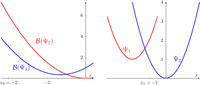
Figure 4: Illustration of the multistage (two stages here) optimization problem studied in §5.2. The final cost function, $\psi=\inf(\psi_{1},\psi_{2})$ is shown in the right subfigure and displays of the images, by the Bellman operator $\mathcal{B}$, of the functions $\psi_{1}$ and $\psi_{2}$ are drawn in the left subfigure. We have that $\mathcal{B}(\psi_{2})(x_{0})>\mathcal{B}(\psi_{1})(x_{0})$. At the final time $t=1$, the “best function” at the point $-1$ is $\psi_{2}$. The image by the $k$-th optimal dynamic of $x_{0}=-2$ is $x_{1}=-1$.

We consider a (non-homogeneous) problem with only two time steps, that is $T=1$ and $t\in\left\{0,1\right\}$ such that

$\bullet$ The state space $\mathbb{X}$ and the control space $\mathbb{U}$ are equal to $\mathbb{R}$.

$\bullet$ The linear dynamic is $f(x,u)=x+u$.

$\bullet$ The quadratic cost is $c(x,u)=x^{2}+u^{2}$.

$\bullet$ The final cost function is the infimum, $\psi=\inf(\psi_{1},\psi_{2})$, of two given quadratic mappings, $\psi_{1}(x)=(x+2)^{2}+1$ and $\psi_{2}(x)=x^{2}$.

The Bellman operator $\mathcal{B}$, associated to this multistage optimization problem is defined for every $\phi:\mathbb{X}\to\overline{\mathbb{R}}$ and every $x\in\mathbb{X}$ by

$$\mathcal{B}(\phi)(x)=\min_{u\in U}\big{(}x^{2}+u^{2}+\phi(x+u)\big{)}=x^{2}+\min_{u\in U}\big{(}u^{2}+\phi(x+u)\big{)}\;.$$

For the case where $\phi_{a,b}(\cdot)=(\cdot+a)^{2}+b$ with $a,b\in\mathbb{R}$ one has for every $x\in\mathbb{R}$

$$\mathcal{B}(\phi_{a,b})(x)=\frac{3}{2}x^{2}+ax+b.$$ (47)

Fix $x_{0}=x_{0}^{k}=-2$ for every $k\in\mathbb{N}$. As described in Algorithm 1, the approximations of the value functions $V_{1}$ and $V_{0}$ are initialized to $+\infty$. Thus every control $u\in\mathbb{U}$ is optimal in the sense that $u\in\mathop{\arg\min}_{u^{\prime}\in\mathbb{U}}x^{2}+(u^{\prime})^{2}+\phi(x+u^{\prime})$. Hence if we set $x_{1}^{0}:=-1=f(x_{0},1)$ then $(x_{0},x_{1}^{0})$ is an optimal trajectory as described in Proposition 20.

We deduce from Equation (47) the following facts, illustrated in Figure 4.

1. The image of $\psi_{2}$ is strictly greater than the image of $\psi_{1}$ by the Bellman operator $\mathcal{B}$, i.e.

   $$\mathcal{B}(\psi_{2})(-2)>\mathcal{B}(\psi_{1})(-2).$$

2. The image by the $k$-th optimal dynamic of $-2$ is $-1$, i.e. setting $u_{0}^{k}:=\mathop{\arg\min}_{u^{\prime}\in\mathbb{U}}(-2)^{2}+(u^{\prime})^{2}+V_{1}^{k}(-2+u^{\prime})$ (the $\mathop{\arg\min}$ is here a singleton) one has

   $$f(-2,u_{0}^{k})=-1.$$

3. At the final step $t=1$, the best function at the point $-1$ is $\psi_{2}$, i.e.

   $$\psi(-1)=\inf(\psi_{1}(-1),\psi_{2}(-2))=\psi_{2}(-2).$$

From those three facts, one can deduce starting $x_{0}=-2$ and $x_{1}=-1$, the optimal trajectory for the current approximations will always be sent to $x_{1}=-1$. But, as shown in the proof of Proposition 29 one can show that the image by $\mathcal{B}$ of an infimum is the infimum of the images by $\mathcal{B}$:

$$V_{0}(-2)=\mathcal{B}(\inf(\psi_{1},\psi_{2}))(-2)=\inf(\mathcal{B}(\psi_{1})(-2),\mathcal{B}(\psi_{1})(-2)).$$

Thus for every $k\in\mathbb{N}$, we have $V_{0}(-2)=\mathcal{B}(\psi_{1})(-2)<\mathcal{B}(\psi_{1})(-2)=V_{0}^{k}(-2)$. The constant sequence $V_{0}^{k}(-2)$ fails to converge to $V_{0}(-2)$.

6 Numerical experiments on a toy example

In §6.1, we propose a toy optimization Problem (48) on which we run TDP-SDDP and TDP-Minplus. Problem (48) falls in the framework described in Section 4. Thus, we are able to obtain lower approximations of $V_{t}$ using TDP-SDDP. TDP-Minplus cannot be applied directly. We apply a “discretization” step to Problem (48) (see §6.2) which yields Problem (49) parameterized by an integer $N>0$. Then we apply to Problem (49) an “homogenization” step (see §6.3) to obtain Problem (50). The value functions $V_{t}$ of the original Problem (48) are bounded from above by $\widetilde{V}_{t,N}$, the value functions of Problem (50). We apply TDP-Minplus (described in Section 5) to Problem (50) which gives upper approximations of $\widetilde{V}_{t,N}$ and a fortiori, of $V_{t}$. In §6.6, we show numerical experiments which show the convergence of this approximation scheme to $V_{t}$.

6.1 A toy example: constrained linear-quadratic framework

Let $\beta,\gamma$ be two given reals such that $\beta<\gamma$, we study the following multistage linear quadratic problem involving a constraint on one of the controls:

$$\min_{(x,u,v)\in\mathbb{X}^{T+1}\times\mathbb{U}^{T}\times[\beta,\gamma]^{T}} \sum_{t=0}^{T-1}c_{t}(x_{t},u_{t},v_{t})+\psi(x_{T})$$ (48a)

s.t. $$\quad x_{0}\in\mathbb{X}\ \text{given, and}\quad\forall t\in[\![0,T-1]\!],\ x_{t+1}=f_{t}(x_{t},u_{t},v_{t})\;,$$ (48b)

where $\mathbb{X}=\mathbb{R}^{n}$ and $\mathbb{U}=\mathbb{R}^{m}$, with quadratic convex costs functions of the form

$$c_{t}(x,u,v)=x^{T}C_{t}x+u^{T}D_{t}u+v^{2}d_{t},$$

where $C_{t}\in\mathbb{S}^{+}_{n}$, $D_{t}\in\mathbb{S}^{++}_{n}$ and $d_{t}>0$, linear dynamics $f_{t}(x,u,v)=A_{t}x+B_{t}u+vb_{t}$, where $A_{t}$ (resp. $B_{t}$) is a $n\times n$ (resp. $n\times m$) matrix, $b_{t}\in\mathbb{X}$, and final cost function $\psi:=x^{T}Mx$ with $M\in\mathbb{S}^{++}_{n}$.

For every $t\in[\![0,T]\!]$, the value function $V_{t}$ is $L_{t}$-Lipschitz continuous and convex. Moreover the Lipschitz constant $L_{t}>0$ can be explicitly computed. As done in Section 4 we will generate lower approximations of the value functions $V_{t}$ through compatible selection functions $(\phi_{t}^{\text{\tiny SDDP}})_{t\in[\![0,T]\!]}$. In this example, the structural Assumption 1 are not satisfied as the sets of states and controls are not compacts. As we will still observe convergence of the lower approximations generated by TDP$(\phi_{t}^{\text{\tiny SDDP}})_{t\in[\![0,T]\!]}$ to the value functions, this suggests that the (classical) framework presented in Section 4 can be extended. This will be the object of a future work and here we would like to stress on the numerical scheme and results.

6.2 Discretization of the constrained control

We approximate Problem (48) by discretizing the constrained control in order to obtain an unconstrained switched multistage linear quadratic problem. More precisely, we fix an integer $N\geq 2$, set $v_{i}=\beta+i\frac{\gamma-\beta}{N-1}$ for every $i\in[\![0,N-1]\!]$ and set $\mathbb{V}:=\left\{v_{0},v_{1},\ldots v_{N-1}\right\}$. Then, we define the following unconstrained switched multistage linear quadratic problem:

$$\min_{(x,u,v)\in\mathbb{X}^{T+1}\times\mathbb{U}^{T}\times\mathbb{V}^{T}} \sum_{t=0}^{T-1}c_{t}^{v_{t}}(x_{t},u_{t})+\psi(x_{T})$$ (49a)

s.t. $$\quad x_{0}\in\mathbb{X}\ \text{given, and}\quad\forall t\in[\![0,T-1]\!],\ x_{t+1}=f_{t}^{v_{t}}(x_{t},u_{t})\;,$$ (49b)

where for every $v\in\mathbb{V}$, $f_{t}^{v}=f_{t}(\cdot,\cdot,v)$ and $c_{t}^{v}=c_{t}(\cdot,\cdot,v)$. As the set of controls of Problem (48) contains the set of controls of Problem (49), upper approximations of the value functions of Problem (49) will are give upper approximations of the value functions of Problem (48). Thus we will construct upper approximations for Problem (49).

6.3 Homogenization of the costs and dynamics

We add a dimension to the state space in order to homogenize the costs and dynamics, when a sequence of switching controls is fixed. Define the following homogenized costs and dynamics for every $t\in[\![0,T-1]\!]$ by:

$$\tilde{f_{t}}^{v}(x,y,u) =\begin{pmatrix}A_{t}&vb_{t}\\ 0&1\end{pmatrix}\begin{pmatrix}x\\ y\end{pmatrix}+\begin{pmatrix}B_{t}\\ 0\end{pmatrix}u,$$

$$\tilde{c_{t}}^{v}(x,y,u) =\begin{pmatrix}x\\ y\end{pmatrix}^{T}\begin{pmatrix}C_{t}&0\\ 0&v^{2}d_{t}\end{pmatrix}\begin{pmatrix}x\\ y\end{pmatrix}+u^{T}D_{t}u,$$

And as the final cost function is already homogeneous, $\widetilde{\psi}(x,y)=\begin{pmatrix}x\\ y\end{pmatrix}^{T}\begin{pmatrix}M&0\\ 0&0\end{pmatrix}\begin{pmatrix}x\\ y\end{pmatrix}$. Using these homogenized functions we define a multistage optimization problem with one more (compared to Problem (49)) dimension on the state variable:

$$\min_{{(x,y,u,v)\in\mathbb{X}^{T+1}\times\mathbb{R}^{T+1}\times\mathbb{U}^{T}\times\mathbb{V}^{T}}}\sum_{t=0}^{T-1}\tilde{c_{t}}^{v_{t}}(x_{t},y_{t},u_{t})+\widetilde{\psi}(x_{T},y_{T})$$ (50)

$$\text{s.t.}\ \left\{\begin{aligned} &(x_{0},y_{0})\in\mathbb{X}\times\mathbb{R}\ \text{is given,}\\ &\forall t\in[\![0,T-1]\!],\ (x_{t+1},y_{t+1})=\tilde{f_{t}}^{v_{t}}(x_{t},y_{t},u_{t})\;.\\ \end{aligned}\right.$$

One can deduce the value functions $V_{t,N}$ of the multistage optimization problem (49) (with non-homogeneous costs and dynamics) from the value functions $\widetilde{V}_{t,N}$ of (50) (with homogeneous costs and dynamics) by Proposition 34. For every $x\in\mathbb{X}$, we have that

$$V_{t,N}(x)=\widetilde{V}_{t,N}(x,1)\;.$$ (51)

For every time step $t\in[\![0,T]\!]$ the value function $\widetilde{V}_{t,N}$ solution of Problem (50) is $2$-homogeneous. That is, for every $(x,y)\in\mathbb{X}\times\mathbb{R}$ and every $\lambda\in\mathbb{R}$, we have $\widetilde{V}_{t,N}\left(\lambda x,\lambda y\right)=\lambda^{2}\widetilde{V}_{t,N}\left(x,y\right).$ This will allow us to restrict the study of the value functions to the unit sphere, which is compact.

6.4 Min-plus upper approximations of the value functions of Problem (50)

We apply the results of Section 5 as follows. Let $v\in\mathbb{V}$ be a given switching control, in this framework, the operator $\mathcal{B}_{t}^{v}$ is defined as in Section 5 but with an augmented state. More precisely, for every function $\phi:\mathbb{X}\times\mathbb{R}\to\overline{\mathbb{R}}$ and every point $(x,y)\in\mathbb{X}\times\mathbb{R}$:

$$\mathcal{B}_{t}^{v}\left(\phi\right)(x,y)=\inf_{u\in\mathbb{U}}\tilde{c}_{t}^{v}(x,y,u)+\lVert\tilde{f}_{t}^{v}(x,y,u)\rVert^{2}\phi(\frac{\tilde{f}_{t}^{v}(x,y,u)}{\lVert\tilde{f}_{t}^{v}(x,y,u)\rVert})\;.$$

Then, for every time $t\in[\![0,T-1]\!]$, the Dynamic Programming operator $\mathcal{B}_{t}$ associated to Problem (50) satisfies $\mathcal{B}_{t}\left(\phi\right):=\inf_{v\in\mathbb{V}}\mathcal{B}_{t}^{v}\left(\phi\right)$.

A key property of the operators $\mathcal{B}_{t}^{v}$ and $\mathcal{B}_{t}$ is that they are min-additive, meaning that for every functions $\phi_{1},\phi_{2}:\mathbb{X}\to\overline{\mathbb{R}}$ one has:

$$\mathcal{B}_{t}^{v}\big{(}\inf(\phi_{1},\phi_{2})\big{)}=\inf\big{(}\mathcal{B}_{t}^{v}(\phi_{1}),\mathcal{B}_{t}^{v}(\phi_{2})\big{)}\enspace,$$

and a similar equation for $\mathcal{B}_{t}$. Moreover, by Riccati formula (see Equation (52)), the image of a convex quadratic function by $\mathcal{B}_{t}^{v}$ is also a convex quadratic function.

Lemma 26 suggests to use the following set of basic functions:

$$\mathbf{F}_{t}^{\text{\tiny min-plus}}:=F_{t}\ \text{ and }\ \mathbb{F}_{t}^{\text{\tiny min-plus}}:=\left\{\mathcal{V}_{F}\ \Big{|}\ F\subset\mathbf{F}_{t}^{\text{\tiny min-plus}}\right\}\;.$$

As done in Section 5, one could also have considered as basic functions the quadratic functions bounded in the Loewner sense between $0$ and $\alpha_{t}\mathrm{I}$, where $\alpha_{t}>0$, $t\in[\![0,T]\!]$, are real numbers such that, if $\phi$ is a quadratic form bounded between $0$ and $\alpha_{t+1}\mathrm{I}$, then $\mathcal{B}_{t}^{v}(\phi)$ is bounded between $0$ and $\alpha_{t}\mathrm{I}$.

Moreover, using the aforementioned properties, one will be able to compute $\mathcal{B}_{t}^{v}(\mathcal{V}_{F})$ for a given switching control $v$ and $\mathcal{B}_{t}(\mathcal{V}_{F})$, for any finite set $F$ of convex quadratic functions. Therefore, given a time $t\in[\![0,T-1]\!]$, we define the selection function $\phi_{t}^{\text{\tiny min-plus}}$ as follows. For any given $F\subset\mathbf{F}_{t+1}^{\text{\tiny min-plus}}$ and $(x,y)\in\mathbb{X}\times\mathbb{R}$,

$$\phi_{t}^{\text{\tiny min-plus}}\left(F,x,y\right)=\mathcal{B}_{t}^{v}(\phi)$$

$$\text{for some}\quad(v,\phi)\in\mathop{\arg\min}_{(v,\phi)\in\mathbb{V}\times F}\mathcal{B}_{t}^{v}\left(\phi\right)\left(x,y\right).$$

Moreover, at time $t=T$, for any $F\subset\mathbf{F}_{T}^{\text{\tiny min-plus}}$ and $(x,y)\in\mathbb{X}\times\mathbb{R}$, we set

$$\phi_{t}^{\text{\tiny min-plus}}\left(F,x,y\right)=\widetilde{\psi}(x,y)=\psi(x).$$

Motivated by the 2-homogeneity of the value functions, the random draws of TDP for the basic functions $\mathbf{F}_{t}^{\text{\tiny min-plus}}$, $1\leq t\leq T$ and the selection functions $\phi_{t}^{\text{\tiny min-plus}}$ will be made uniformly on the unit euclidean sphere, which satisfies Definition 5. Indeed, by $2$-homogeneity, it is enough to know the value functions of (50) on the sphere to know them on the whole state space.

6.5 Upper and lower approximations of the value functions

For a large number of discretization points $N$ (defined in §6.2), one would expect that the value functions $V_{t,N}$ of (49) approximate the value functions $V_{t}$ of (48). Indeed, one can show that for every time step $t\in[\![0,T]\!]$, the approximation error is bounded by $C_{t}T/N^{2}$ in $\mathbb{X}$, for some constant $C_{t}>0$. Thus, for large $N$, we have $V_{t,N}\approx V_{t}$ and by Equation (51), for every $N\geq 2$, we have

$$\widetilde{V}_{t,N}(\cdot,1)=V_{t,N}\geq V_{t}.$$

In the following Proposition we approximate $\widetilde{V}_{t,N}$ from above by a min-plus algorithm and $V_{t}$ from below by SDDP and using the convergence result of Theorem 13 (admitting that the result still holds for SDDP in this framework), we obtain the following one.

Theorem 31

For every $t\in[\![0,T]\!]$, denote by $\left(\overline{V}_{t}^{k}\right)_{k\in\mathbb{N}}$ (resp. $(\underline{V}_{t}^{k})_{k\in\mathbb{N}}$) the sequence of functions generated by TDP with the selection function $\phi_{t}^{\text{\tiny min-plus}}$ (resp. $\phi_{t}^{\text{\tiny SDDP}}$) and the draws made uniformly over the euclidean sphere of $\mathbb{X}\times\mathbb{R}$ (resp. made as described in Proposition 20).

Then the sequence $\left(\overline{V}_{t}^{k}\right)_{k\in\mathbb{N}}$ (resp. $(\underline{V}_{t}^{k})_{k\in\mathbb{N}}$) is non-increasing (resp. non-decreasing), bounded from below (resp. above) by $\widetilde{V}_{t,N}$ (resp. $V_{t}$) and converges uniformly to $\widetilde{V}_{t,N}$ (resp. $V_{t}$) on any compact subset of $\mathbb{X}\times\mathbb{R}$ (resp. $K_{t}^{*}$ defined in Proposition 20).

6.6 Numerical experiments

The following data was used as a specific case of (48). For every time $t\in[\![0,T-1]\!]$,

$$A_{t} =(1-0.1)\;\mathrm{Id}\quad B_{t} =\begin{pmatrix}1&\cdots&1\\ \vdots&&\vdots\\ 1&\cdots&1\end{pmatrix}\quad b_{t} =\begin{pmatrix}1\\ \vdots\\ 1\end{pmatrix}$$

$$C_{t} =0.1\;\mathrm{Id}\quad D_{t} =0.1\;\mathrm{Id}\quad d_{t} =0.1.$$

The time horizon is $T=15$, the states are in $\mathbb{X}=\mathbb{R}^{n}$ with $n=25$, the unconstrained continuous controls are in $\mathbb{U}=\mathbb{R}^{m}$ with $m=3$, the constrained continuous control is in $[\beta,\gamma]$, with $[\beta,\gamma]=[1,5]$ in the first example and $[\beta,\gamma]=[-3,5]$ in the second one. Moreover, we start from the initial point $x_{0}=0.2\;(1,\ldots,1)^{T}$ when TDP is applied with the selection function $\phi_{t}^{\text{\tiny SDDP}}$ and the number of discretization points $N$ is varying from $5$ to $200$, for TDP with the selection function $\phi_{t}^{\text{\tiny min-plus}}$. In Figures 5 and 6, we give graphs representing the values $\underline{V}_{t}^{k}(x_{t}^{k})$ and $\overline{V}_{t}^{k}(x_{t}^{k},1)$ at each time step $t\in[\![0,T-1]\!]$ where the sequence of states $(x_{t}^{k})_{k\in\mathbb{N}}$ is the optimal trajectory for the current lower approximations $(\underline{V}_{t}^{k})_{k\in\mathbb{N}}$ defined in (20). From Theorem 31, we know that for every $t\in[\![0,T-1]\!]$ the gap $\overline{V}_{t}^{k}(x_{t}^{k},1)-\underline{V}_{t}^{k}(x_{t}^{k})$ should be close to $0$ as $k$ increases assuming that $N$ is large enough to have $V_{t}\approx V_{t,N}$.

Figure 5: First example for $\beta=1$, $\gamma=5$ with $N=5$ after $7$ iterations (left), $18$ iterations (middle) and $40$ iterations (right).

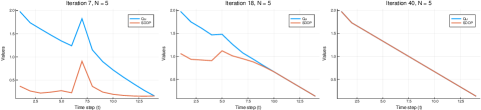
Figure 6: Second example for $\beta=-3$, $\gamma=5$ with varying $N=5$ (left), $N=50$ (middle) and $N=200$ (right) after $20$ iterations.

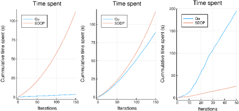
Figure 7: Time spent for the first example (left) and the second example when $N=50$ (middle) and $N=200$ (right).

On those two examples, we exhibit two convergence behaviors. On the first example, the constrained control has to be greater than $1$, thus avoiding $0$ which would have been (or almost) the optimal control if there were no constraint. The optimal constrained control is the projection on $\mathbb{U}\times[\beta,\gamma]$ of the optimal unconstrained control, thus the switching control is most of the time equal to the lower bound $\beta=1$.

From this observation we deduce two properties. First, the upper approximation given by Qu algorithm is good, even for a small $N$, as the optimal switch is (most of the time) equal to $\beta$. Second, this implies that at iteration $k$, the set $F_{t}^{k}$ is of small cardinality.

Moreover, in this example the number of switches is $N=5$ thus few computations of $\mathcal{B}_{t}^{v}(\phi)(x)$ need to be done in order to compute $\mathcal{B}_{t}(\phi)(x)$ for some $x\in\mathbb{X}$ and $\phi\in F_{t}^{k}$. Thus, as shown on the left of Figure 7, the computation time of an iteration of Qu’s min-plus algorithm is small compared to SDDP which does not exploit this property.

On the second example, the constrained control is in an interval containing $0$. The switching control often changes and this means more computations. A compromise between computational time and precision can be achieved (see Figure 7) in order to make the computational time of Qu algorithm similar to the one of SDDP algorithm.

Conclusion

In this article we have devised an algorithm, Tropical Dynamic Programming, that encompasses both a discrete time version of Qu’s min-plus algorithm and the SDDP algorithm in the deterministic case. We have shown in the last section that Tropical Dynamic Programming can be applied to two natural frameworks: one for min-plus and one for SDDP. In the case where both framework intersects, one could apply Tropical Dynamic Programming with the selection functions $\phi_{t}^{\text{\tiny min-plus}}$ and get non-increasing upper approximations of the value function. Simultaneously, by applying Tropical Dynamic Programming with the selection function $\phi_{t}^{\text{\tiny SDDP}}$, one would get non-decreasing lower approximations of the value function. Moreover, we have shown that the upper approximations are, almost surely, asymptotically equal to the value function on the whole space of states $\mathbb{X}$ and that the lower approximations are, almost surely, asymptotically equal to the value function on a set of interest.

Thus, in those particular cases we get converging bounds for $V_{0}(x_{0})$, which is the value of the multistage optimization Problem 1, along with asymptotically exact minimizing policies. In those cases, we have shown a possible way to address the issue of computing efficient upper bounds when running the SDDP algorithm by running in parallel another algorithm (namely TDP with min-plus selection functions).

In Section 6 we studied a way to simultaneously build lower and upper approximations of the value functions using the results of the previous sections. However the discretization and homogenization scheme that was described is rapidly limited by the dimension of the control space, due to the need to discretize the constrained controls. We will provide in a future work, a systematic scheme to use simultaneously SDDP and a min-plus methods which is more efficient numerically and does not rely on discretization of the control space. Moreover we will extend the current framework to multistage stochastic optimization problems with finite white noises.

Appendix A Algebraic Riccati Equation

This section gives complementary results for Section 5. We use the same framework and notations introduced in Section 5.

Proposition 32

Fix a discrete control $v\in\mathbb{V}$ and a time step $t\in[\![0,T-1]\!]$.

• The operator $\mathcal{B}_{t}^{v}:\mathbb{S}_{n}\to\mathbb{S}_{n}^{+}$ restricted to the pure quadratic forms (identified with $\mathbb{S}_{n}$ the space of the symmetric semidefinite positive matrices) is given by the discrete time algebraic Riccati equation

  $$\mathcal{B}_{t}^{v}(M)=C_{t}^{v}+(A_{t}^{v})^{T}MA_{t}^{v}-(A_{t}^{v})^{T}MB_{t}^{v}\big{(}D_{t}^{v}+B_{t}^{v}M(B_{t}^{v})^{T}\big{)}^{-1}(B_{t}^{v})^{T}MA_{t}^{v}\;.$$ (52)

• Moreover, when $M\in\mathbb{S}_{n}^{+}$ Equation (52) can be rewritten as

  $$\mathcal{B}_{t}^{v}(M)=\left(A_{t}^{v}\right)^{T}M\left(I+B_{t}^{v}\left(D_{t}^{v}\right)^{-1}\left(B_{t}^{v}\right)^{T}M\right)^{-1}A_{t}^{v}+C_{t}^{v}.$$ (53)

Proof.

$\bullet$ We prove Equation (52). Note that if $M$ is symmetric, then $\mathcal{B}_{t}^{v}(M)$ is also symmetric. Now, let $t\in\left\{T{-}1,T{-}2,\ldots,0\right\}$ and $M\in\mathbb{S}_{n}$ be fixed. Let $x\in\mathbb{X}$, we have that

$$\mathcal{B}_{t}^{v}(M)(x) =\inf_{u\in\mathbb{U}}x^{T}C_{t}^{v}x+u^{T}D_{t}^{v}u+\lVert f_{t}^{v}\left(x,u\right)\rVert^{2}\frac{f_{t}^{v}\left(x,u\right)^{T}}{\lVert f_{t}^{v}\left(x,u\right)\rVert}M\frac{f_{t}^{v}\left(x,u\right)}{\lVert f_{t}^{v}\left(x,u\right)\rVert}$$

$$=\inf_{u\in\mathbb{U}}x^{T}C_{t}^{v}x+u^{T}D_{t}^{v}u+f_{t}^{v}\left(x,u\right)^{T}Mf_{t}^{v}(x,u)$$

$$=x^{T}C_{t}^{v}x+\inf_{u\in\mathbb{U}}u^{T}D_{t}^{v}u+f_{t}^{v}(x,u)^{T}Mf_{t}^{v}(x,u).$$ (54)

As $u\mapsto f_{t}^{v}(x,u)$ is linear, $D_{t}^{v}\succ 0$ and $M\succeq 0$, we have that

$$g:u\in\mathbb{U}\mapsto u^{T}D_{t}^{v}u+f_{t}^{v}(x,u)^{T}Mf_{t}^{v}(x,u)\in\mathbb{R}$$

is strictly convex, hence is minimal when $\nabla g(u)=0$ i.e. for $u\in\mathbb{U}$ such that:

$$\big{(}D_{t}^{v}+\left(B_{t}^{v}\right)^{T}MB_{t}^{v}\big{)}u+(B_{t}^{v})^{T}M(A_{t}^{v})x=0\;.$$ (55)

Now we will show that $D_{t}^{v}+\left(B_{t}^{v}\right)^{T}MB_{t}^{v}$ is invertible. As $M\in\mathbb{S}_{n}$ and $D_{t}^{v}\in\mathbb{S}_{n}^{+}$, for every $u\in\mathbb{U}$, we have:

$$u^{T}\big{(}D_{t}^{v}+(B_{t}^{v})^{T}MB_{t}^{v}\big{)}u=\underbrace{u^{T}D_{t}^{v}u}_{>0}+\underbrace{\left(B_{t}^{v}u\right)^{T}M\left(B_{t}^{v}u\right)}_{\geq 0}>0\;.$$

We have shown that the symmetric matrix $D_{t}^{v}+\left(B_{t}^{v}\right)^{T}MB_{t}^{v}$ is definite positive and thus invertible. We conclude that Equation (55) is equivalent to:

$$u=-\big{(}D_{t}^{v}+(B_{t}^{v})^{T}MB_{t}^{v}\big{)}^{-1}\left(B_{t}^{v}\right)^{T}M\left(A_{t}^{v}\right)x\;.$$ (56)

Finally, replacing Equation (56) in Equation (54) we get after simplifications that

$$\mathcal{B}_{t}^{v}(M)(x) =x^{T}\Big{(}C_{t}^{v}+(A_{t}^{v})^{T}MA_{t}^{v}$$

$$\hskip 28.45274pt-(A_{t}^{v})^{T}MB_{t}^{v}\big{(}D_{t}^{v}+(B_{t}^{v})^{T}MB_{t}^{v}\big{)}^{-1}(B_{t}^{v})^{T}MA_{t}^{v}\Big{)}x\;,$$

which gives Equation (52).

$\bullet$ Equation (53) follows from [9, Proposition 12.1.1 page 271]. $\Box$

Appendix B Smallest and greatest eigenvalues

Here we recall some formulas on the lowest and greatest eigenvalues of a matrix. Denote the smallest eigenvalue of a symmetric real matrix $M$ by $\lambda_{\tiny\text{min}}(M)$ (every eigenvalue of $M$ is real) and by $\lambda_{\tiny\text{max}}(M)$ its greatest eigenvalue.

Proposition 33

Let $n>0$ be given. We have the following matrix inequalities.

$$\forall(A,B)\in\mathbb{S}_{n}^{2}\;,\enspace\lambda_{\tiny\text{max}}(A+B)\leq\lambda_{\tiny\text{max}}(A)+\lambda_{\tiny\text{max}}(B)\;.$$ (57a)

$$\forall(A,B)\in\mathbb{M}_{n}{\times}\mathbb{S}_{n}\;,\enspace\lambda_{\tiny\text{max}}(A^{T}BA)\leq\lambda_{\tiny\text{max}}(A^{T}A)\lambda_{\tiny\text{max}}(B)\;.$$ (57b)

Proof. For any matrix $M\in\mathbb{M}_{n}$, the spectral norm of $M$, ${\lVert M\rVert}_{\text{sp}}$, (See [4, Theorem 1.4.2]) is the subordinate matrix norm of the euclidean norm on $\mathbb{R}^{n}$. When the matrix $M\in\mathbb{S}_{n}$ is real symmetric, we have that ${\lVert M\rVert}_{\text{sp}}=\lambda_{\tiny\text{max}}(M)$ and for any real matrix $M\in\mathbb{M}_{n}$, we have that $\lambda_{\tiny\text{max}}(M^{T}M)=\lambda_{\tiny\text{max}}(MM^{T})=\lVert M\rVert^{2}$.

$\bullet$ Fix $A,B\in\mathbb{S}_{n}$, we prove Equation (57a). As $A+B\in\mathbb{S}_{n}$ and using the fact that a subordinate matrix norm is a norm we have that $\lambda_{\tiny\text{max}}(A+B)={\lVert A+B\rVert}_{\text{sp}}\leq{\lVert A\rVert}_{\text{sp}}+{\lVert B\rVert}_{\text{sp}}=\lambda_{\tiny\text{max}}(A)+\lambda_{\tiny\text{max}}(B)$.

$\bullet$ Fix $(A,B)\in\mathbb{M}_{n}{\times}\mathbb{S}_{n}$. We prove Equation (57b) as follows

$$\lambda_{\tiny\text{max}}(A^{T}BA) =\lVert A^{T}BA\rVert A^{T}BA\in\mathbb{S}_{n}$$ (as )

$$\leq{\lVert A^{T}\rVert}_{\text{sp}}{\lVert B\rVert}_{\text{sp}}{\lVert A\rVert}_{\text{sp}} {\lVert\cdot\rVert}_{\text{sp}}$$ ( is submultiplicative as a matrix norm)

$$={\lVert A\rVert}_{\text{sp}}^{2}{\lVert B\rVert}_{\text{sp}}=\lambda_{\tiny\text{max}}(A^{T}A)\lambda_{\tiny\text{max}}(B)\;.$$

This ends the proof. $\Box$

Appendix C Homogenization

We explain why, by adding another dimension to the state variable, there is no loss of generality induced by studying pure quadratic forms in Problem 37 instead of positive polynomial of degree $2$, nor is there one for studying linear dynamics instead of affine dynamics.

First, we define the operator ${\mathcal{H}}_{2}$ that maps a function $\phi$ defined on a finite dimensional vector space $\mathbb{E}$ to a $2$-homogeneous function ${\mathcal{H}}_{2}\big{(}\phi\big{)}$ defined on the extended domain $\mathbb{E}\times\mathbb{R}$ as follows

$$\begin{array}[]{ccll}{\mathcal{H}}_{2}:&\overline{\mathbb{R}}^{\mathbb{E}}&\longrightarrow&\overline{\mathbb{R}}^{\mathbb{E}\times\mathbb{R}}\\ &\phi&\longmapsto&{\mathcal{H}}_{2}\big{(}\phi\big{)}:(z,y)\mapsto y^{2}\phi(\frac{z}{y})\ \text{if}\ y\neq 0,\ 0\ \text{otherwise}.\end{array}$$ (58)

Thus, if $\phi$ is a positive polynomial of degree $2$, then ${\mathcal{H}}_{2}(\phi)$ is a $2$-homogeneous convex quadratic form (with possibly a mixed term in $x$ and $u$). In a similar way, we define the operator ${\mathcal{H}}_{1}$ that maps any function $\phi$ defined on a domain $\mathbb{E}$ and taking values in $\mathbb{E}$ to a $1$-homogeneous function ${\mathcal{H}}_{1}\big{(}\phi\big{)}$ as follows

$$\begin{array}[]{ccll}{\mathcal{H}}_{1}:&\mathbb{E}^{\mathbb{E}}&\longrightarrow&(\mathbb{E}\times{\mathbb{R}})^{\mathbb{E}\times{\mathbb{R}}}\\ &\phi&\longmapsto&{\mathcal{H}}_{1}\big{(}\phi\big{)}:(z,y)\mapsto(y\phi(\frac{z}{y}),y)\ \text{if}\ y\neq 0,\ 0\ \text{otherwise}.\end{array}$$ (59)

Now consider $\left(\mathcal{B}_{t}\right)_{t\in[\![0,T-1]\!]}$ the Bellman operators associated to Problem 37

$$\begin{array}[]{ccll}\mathcal{B}_{t}:&\overline{\mathbb{R}}^{\mathbb{X}}&\longrightarrow&\overline{\mathbb{R}}^{\mathbb{X}}\\ &\phi&\longmapsto&\mathcal{B}_{t}\big{(}\phi\big{)}:x\mapsto\min_{\begin{subarray}{c}u\in\mathbb{U}\\ v\in\mathbb{V}\end{subarray}}c_{t}^{v}(x,u)+\phi(f_{t}^{v}(x,u))\;,\end{array}$$ (60)

We denote by $(\mathcal{B}_{t}^{{\mathcal{H}}})_{t\in[\![0,T-1]\!]}$, the family of Bellman operators obtained through homogenization (with $\mathbb{E}=\mathbb{X}\times\mathbb{U}$) as follows

$$\begin{array}[]{ccll}\mathcal{B}_{t}^{{\mathcal{H}}}:&\overline{\mathbb{R}}^{\mathbb{X}\times{\mathbb{R}}}&\longrightarrow&\overline{\mathbb{R}}^{\mathbb{X}\times{\mathbb{R}}}\\ &\varphi&\longmapsto&\mathcal{B}_{t}^{{\mathcal{H}}}\big{(}\varphi\big{)}:(x,y)\mapsto\min_{\begin{subarray}{c}u\in\mathbb{U}\\ v\in\mathbb{V}\end{subarray}}{\mathcal{H}}_{2}\big{(}c_{t}^{v}\big{)}\big{(}x,u,y\big{)}\\ &&&\hskip 85.35826pt+\varphi({\mathcal{H}}_{1}\big{(}f_{t}^{v}\big{)}(x,u,y)).\end{array}$$ (61)

The next proposition relates the solution of Problem 37 with non-homogeneous functions to the solution of the associated homogenized problem.

Proposition 34

Let $(V_{t})_{t\in[\![0,T]\!]}$ (resp. $(\widetilde{V}_{t})_{t\in[\![0,T]\!]}$) denote the solutions of the Dynamic Programming Equation (3) system of equations associated with the operators $(\mathcal{B}_{t})_{t\in[\![0,T-1]\!]}$ defined by Equation (60) (resp. $(\mathcal{B}^{{\mathcal{H}}}_{t})_{t\in[\![0,T-1]\!]}$ defined by Equation (61)) and final cost $\psi$ (resp. ${\mathcal{H}}_{2}\big{(}\psi\big{)}$)). Then, for every $x\in\mathbb{X}$ and $t\in[\![0,T]\!]$ , we have that $V_{t}(x)=\widetilde{V}_{t}(x,1)$.

Proof. First, it is easy to prove by backward recursion on time $t\in[\![0,T]\!]$, that the mappings $\widetilde{V}_{t}$ for every $t\in[\![0,T]\!]$, are $2$-homogeneous. Second, we will show by backward recursion on time that, for every $t\in[\![0,T]\!]$,

$$\widetilde{V}_{t}={\mathcal{H}}_{2}\big{(}V_{t}\big{)}.$$ (62)

Then, the result will follow by evaluating Equation (62) at $y=1$. At the final time $t=T$, we have that

$$\widetilde{V}_{T}:={\mathcal{H}}_{2}\big{(}\psi\big{)}={\mathcal{H}}_{2}\big{(}V_{T}\big{)}.$$

Now, assume that for some $t\in[\![0,T-1]\!]$, we have that $\widetilde{V}_{t+1}={\mathcal{H}}_{2}\big{(}V_{t+1}\big{)}$, for $(x,y)\in\mathbb{X}\times\mathbb{R}$ we successively obtain that

$$\widetilde{V}_{t}(x,y) =\mathcal{B}_{t}^{{\mathcal{H}}}(\widetilde{V}_{t+1})(x,y)$$

$$=\min_{\begin{subarray}{c}u\in\mathbb{U}\\ v\in\mathbb{V}\end{subarray}}{\mathcal{H}}_{2}\big{(}c_{t}^{v}\big{)}(x,u,y)+\widetilde{V}_{t+1}\Big{(}{\mathcal{H}}_{1}\big{(}f_{t}^{v}\big{)}(x,u,y)\Big{)} 2 \widetilde{V}_{t+1}$$ (-homogeneity of )

$$=\min_{\begin{subarray}{c}u\in\mathbb{U}\\ v\in\mathbb{V}\end{subarray}}{\mathcal{H}}_{2}\big{(}c_{t}^{v}\big{)}(x,u,y)+{\mathcal{H}}_{2}\big{(}V_{t+1}\big{)}\Big{(}yf_{t}^{v}(\frac{x}{y},\frac{u}{y}),y\Big{)}$$ (Induction hyp. and def.)

$$=\min_{\begin{subarray}{c}u\in\mathbb{U}\\ v\in\mathbb{V}\end{subarray}}y^{2}c_{t}^{v}(\frac{x}{y},\frac{u}{y})+y^{2}V_{t+1}(f_{t}^{v}(\frac{x}{y},\frac{u}{y}))$$ (by Equation (58))

$$=y^{2}\min_{\begin{subarray}{c}u^{\prime}\in\mathbb{U}\\ v\in\mathbb{V}\end{subarray}}c_{t}^{v}(\frac{x}{y},u^{\prime})+V_{t+1}(f_{t}^{v}(\frac{x}{y},u^{\prime})) u^{\prime}=u/y$$ ()

$$=y^{2}\mathcal{B}_{t}(V_{t+1})(\frac{x}{y})$$

$$={\mathcal{H}}_{2}\big{(}V_{t}\big{)}(x,y)\;.$$ (by Equation (58))

This ends the proof. $\Box$

Lastly, we briefly explain how to get rid of the possible mixed terms in both $u$ and $x$ in the cost functions after homogenization. That is, there is no loss of generality to consider the case of cost functions which are positive polynomials of degree $2$ and affine cost than to consider the case studied in §5.1, i.e. pure quadratic costs and linear functions. From Proposition 34, we have seen that one can consider the case where the cost functions are $2$-homogeneous with linear dynamics. Assume (for the sake of simplicity, we omit the discrete control $v$ here) that the cost function $c_{t}$ is of the form

$$c_{t}(x,u):=x^{T}P_{1}x+x^{T}P_{2}u+u^{T}P_{3}u,$$

where $P_{1}$, $P_{2}$ and $P_{3}$ are symmetric semidefinite positive matrices of coherent dimensions, with $P_{3}$ being definite positive. Moreover, fix a $2$-homogeneous convex quadratic form $\psi$ and assume the dynamic $f_{t}$ to be linear of the form

$$f_{t}(x,u):=Ax+Bu.$$

Setting $Q_{1}:=P_{1}-\frac{1}{4}P_{2}P_{3}^{-1}P_{2}^{T}$, $Q_{2}:=P_{3}$, $L:=\frac{1}{2}P_{3}^{-1}P_{2}^{T}$, one has that the cost function $(x,u)\mapsto c_{t}^{\prime}(x,u):=x^{T}Q_{1}x+u^{T}Q_{2}u$ is a quadratic function without mixing term and $(x,u)\mapsto f_{t}(x,u):=(A+L)x+Bu$ is linear. Furthermore, by straightforward computations, one can check that $c_{t}$ and $f_{t}$ satisfy:

$$c_{t}(x,u+Lx)=c_{t}^{\prime}(x,u)\quad\text{and}\quad f_{t}(x,u+Lx)=f_{t}^{\prime}(x,u).$$ (63)

Note that as $Q_{2}=P_{3}$, the matrix $Q_{2}$ is symmetric definite positive and as $c_{t}$ is positive and by Equation (63) for every $x\in\mathbb{X}$ and $u\in\mathbb{U}$

$$x^{T}Q_{1}x=c_{t}^{\prime}(x,0)=c_{t}(x,0+Lx)\geq 0,$$

then $Q_{1}$ is symmetric semidefinite positive. Thus the quadratic function $c_{t}^{\prime}$ is convex and a pure quadratic form in the sense of Definition 22.

Consider the Bellman operator associated with the costs $c_{t}^{\prime}$ and dynamics $f_{t}^{\prime}$:

$$\begin{array}[]{ccll}\mathcal{B}_{t}^{\prime}:&\overline{\mathbb{R}}^{\mathbb{X}}&\longrightarrow&\overline{\mathbb{R}}^{\mathbb{X}}\\ &\phi&\longmapsto&\mathcal{B}_{t}^{\prime}\big{(}\phi\big{)}:x\mapsto\min_{u\in\mathbb{U}}c_{t}^{\prime}(x,u)+\phi(f_{t}^{\prime}(x,u))\;,\end{array}$$ (64)

Thus, for any function $\phi\in\overline{\mathbb{R}}^{\mathbb{X}}$ and every $x\in\mathbb{X}$, recall that $\mathbb{U}=\mathbb{R}^{m}$ is unconstrained, so we have that

$$\mathcal{B}_{t}(\phi)(x) =\min_{u\in\mathbb{U}}c_{t}(x,u)+\phi(f_{t}(x,u))$$

$$=\min_{u^{\prime}=u+Lx\in\mathbb{U}}c_{t}(x,u+Lx)+\phi(f_{t}(x,u+Lx))$$

$$=\min_{u^{\prime}\in\mathbb{U}}c_{t}^{\prime}(x,u^{\prime})+\phi(f_{t}(x,u^{\prime}))$$

$$\mathcal{B}_{t}(\phi)(x) =\mathcal{B}_{t}^{\prime}(\phi)(x).$$ (65)

From Equation (65), one can deduce by backward recursion (as done in Proposition 34) on the time step $t\in[\![0,T]\!]$, that the value functions $V_{t}$ (resp. $V_{t}^{\prime}$) of the Dynamic Programming problem with Bellman operators $\mathcal{B}_{t}$ (resp. $\mathcal{B}_{t}^{\prime}$) and final cost function $\psi$ (resp. $\psi$ as well) satisfy $V_{t}=V_{t}^{\prime}$   .

References

- [1] Jean Pierre Aubin and Ivar Ekeland. Applied Nonlinear Analysis: Jean-Pierre Aubin and Ivar Ekeland. Pure and Applied Mathematics: A Wiley-Interscience Series of Texts, Monographs, and Tracts. Wiley, New York, 1984.
- [2] Richard Bellman. The theory of dynamic programming. Bulletin of the American Mathematical Society, 60(6):503–515, November 1954.
- [3] Dimitri P. Bertsekas. Dynamic Programming and Optimal Control, volume 1 of Athena Scientific Optimization and Computation Series. Athena Scientific, Belmont, Mass, fourth edition, 2016.
- [4] Philippe G. Ciarlet. Introduction to Numerical Linear Algebra and Optimisation:. Cambridge University Press, first edition, August 1989.
- [5] Stuart Dreyfus. Richard Bellman on the Birth of Dynamic Programming. Operations Research, 50(1):48–51, February 2002.
- [6] P. Girardeau, V. Leclere, and A. B. Philpott. On the Convergence of Decomposition Methods for Multistage Stochastic Convex Programs. Mathematics of Operations Research, 40(1):130–145, February 2015.
- [7] Vincent Guigues. SDDP for some interstage dependent risk-averse problems and application to hydro-thermal planning. Computational Optimization and Applications, 57(1):167–203, January 2014.
- [8] Vincent Guigues and Werner Römisch. Sampling-Based Decomposition Methods for Multistage Stochastic Programs Based on Extended Polyhedral Risk Measures. SIAM Journal on Optimization, 22(2):286–312, January 2012.
- [9] Peter Lancaster and L. Rodman. Algebraic Riccati Equations. Oxford Science Publications. Oxford University Press, 1995.
- [10] William M. McEneaney. A Curse-of-Dimensionality-Free Numerical Method for Solution of Certain HJB PDEs. SIAM Journal on Control and Optimization, 46(4):1239–1276, January 2007.
- [11] M. V. F. Pereira and L. M. V. G. Pinto. Multi-stage stochastic optimization applied to energy planning. Mathematical Programming, 52(1-3):359–375, May 1991.
- [12] Zheng Qu. Nonlinear Perron-Frobenius Theory and Max-plus Numerical Methods for Hamilton-Jacobi Equations. PhD thesis, Ecole Polytechnique X, October 2013.
- [13] Zheng Qu. A max-plus based randomized algorithm for solving a class of HJB PDEs. In 53rd IEEE Conference on Decision and Control, pages 1575–1580, December 2014.
- [14] Ralph Tyrrell Rockafellar and Roger J.-B. Wets. Variational Analysis. Number 317 in Die Grundlehren Der Mathematischen Wissenschaften in Einzeldarstellungen. Springer, Dordrecht, corr. 3. print edition, 2009.
- [15] Laurent Schwartz. Analyse. 1: Théorie Des Ensembles et Topologie. Number 42 in Collection Enseignement Des Sciences. Hermann, Paris, nouv. tirage edition, 1995.
- [16] Alexander Shapiro. Analysis of stochastic dual dynamic programming method. European Journal of Operational Research, 209(1):63–72, February 2011.
- [17] Jikai Zou, Shabbir Ahmed, and Xu Andy Sun. Stochastic dual dynamic integer programming. Mathematical Programming, March 2018.