A Centimeter-wave Study of Methanol and Ammonia Isotopologues in Sgr B2(N): Physical and chemical differentiation between two hot cores

Abstract

We present new radio-frequency interferometric maps of emission from the ¹⁴NH₃, ¹⁵NH₃, and NH₂D  isotopologues of ammonia, and the ¹²CH₃OH  and ¹³CH₃OH  isotopologues of methanol toward Sgr B2(N). With a resolution of $\sim 3^{\prime\prime}$ (0.1 pc), we are able to spatially resolve emission from two hot cores in this source and separate it from absorption against the compact H II  regions in this area. The first (N1) is the well-known v = 64 km s^-1  core, and the second (N2) is a core 6^′′ to the north at v = 73 km s^-1. Using emission from ¹⁵NH₃  and hyperfine satellites of ¹⁴NH₃  metastable transitions we estimate the ¹⁴NH₃  column densities of these sources and compare them to those of NH₂D. We find that the ammonia deuteration fraction of N2 is roughly 10-20 times higher than in N1. We also measure an [¹⁵NH₃/¹⁴NH₃] abundance ratio that is apparently 2-3 times higher in N2 than N1, which could indicate a correspondingly higher degree of nitrogen fractionation in N2. In addition, we find that N2 has a factor of 7 higher methanol abundance than N1. Together, these abundance signatures suggest that N2 is a younger source, for which species characteristic of grain chemistry at low temperatures are currently being actively liberated from ice mantles, and have not yet reached chemical equilibrium in the warm gas phase. The high D abundance and possible high ¹⁵N abundance in NH₃  found in N2 are interesting for studying the potential interstellar origin of abundances in primitive solar system material.

1. Introduction

The Sagittarius B2 (Sgr B2) molecular cloud, with a mass of 3$\times 10^{6}$ M_⊙, is the largest molecular cloud in the central 500 pc of the Galaxy, and one of the largest in the Galaxy as a whole (e.g., Scoville et al., 1975a). The Milky Way’s central black hole lies at a distance of $\sim$ 8.1 kpc (Boehle et al., 2016; Gravity Collaboration et al., 2018), with Sgr B2 believed to be $\sim$130 pc from the center of the Milky Way and located slightly closer to the Sun due to the inclination of the central bar (Reid et al., 2009). It is an active site of star formation, containing numerous signposts of this activity from masers (e.g., Mehringer et al., 1994; Reid et al., 1988) and more than 50 compact and ultra-compact H II  regions (Gaume et al., 1995; De Pree et al., 1998; Zhao & Wright, 2011), most of which are clustered in two massive concentrations of star formation in the northern and middle part of this elongated cloud, which are commonly referred to as Sgr B2(N) and (M). In addition to H II  regions, each of these concentrations hosts hot molecular cores having warm temperatures (100$\leq$ T $\leq$ 300 K; Nummelin et al., 2000; Pei et al., 2000), high densities ($10^{6}<$n$<10^{8}$ cm^-3; Lis et al., 1990; Qin et al., 2011), and high gas phase abundances of complex organic molecules (Miao et al., 1995; Belloche et al., 2008, 2013). Sgr B2 is perhaps best known for its complex chemistry: of the more than 180 known circumstellar and interstellar molecules, half were first detected in Sgr B2 (Snyder et al., 1994), and most of these were detected in line surveys toward the “Large Molecule Heimat” (LMH; where heimat means home in german) hot core in Sgr B2(N).

Because of its enormous column density (N_H2=$10^{24}-10^{25}$ cm^-2; Qin et al., 2011; Schmiedeke et al., 2016) and rich chemistry, the LMH is one of the most well-known hot cores in the Galaxy. Indeed, this core exhibits the most spectral line-dense spectrum of any position in Sgr B2 (Corby et al., 2015). While interferometric observations prior to the Atacama Large Millimeter Array (ALMA) typically only detected the LMH source, centered on Right Ascension = 17^h47^m19.9^s, Declination = -28$\arcdeg$22^′19^′′ at v=63.5 km s^-1  (Vogel et al., 1987; de Vicente et al., 2000), a second line-rich, high-excitation (T${}_{ex}>$80 K) hot core lies $\sim$6^′′ to the north, centered on Right Ascension =17^h47^m19.9^s, Declination = -28$\arcdeg$22^′13^′′ at a velocity of 73 km s^-1  (Belloche et al., 2013; Corby et al., 2015; Halfen et al., 2017). This second core was first noticed in emission from several molecules, including ethyl cyanide (CH₃CH₂CN; Hollis et al., 2003), and the 44 GHz $7_{0}\rightarrow 6_{1}A^{+}$ transition of CH₃OH, in which quasithermal emission is seen in both this source and the LMH (sources h and i respectively; Mehringer & Menten, 1997). Following Belloche et al. (2016), we designate the LMH and the northern hot core as N1 and N2, respectively. Three other, less prominent hot cores in this region (N3, N4, and N5) have also been recently identified in ALMA line observations (Bonfand et al., 2017).

At sub-millimeter wavelengths, the emission from Sgr B2(N) becomes dominated by thermal dust emission from N1 and N2 and their surroundings (Qin et al., 2011; Sánchez-Monge et al., 2017). However, at radio to millimeter wavelengths the continuum emission from Sgr B2(N) is dominated by seven compact, ultracompact, and expanding shell-shaped H II  regions (K1-K7; De Pree et al., 1998, 2015). Both N1 and N2 appear to have an embedded ultra- or hyper-compact H II  region (K2 and K7; Gaume et al., 1995; De Pree et al., 2015), although Bonfand et al. (2017) suggest that the hyper-compact H II  region k7 may be separate from the N2 hot core.

From the sub-millimeter and molecular line emission, N1 and N2 have been measured to have masses ranging from 500 to 5000 M_⊙ (Vogel et al., 1987; de Vicente et al., 2000; Qin et al., 2011), sizes of 0.04 - 0.07 pc (with no apparent fragmentation into smaller structures; Qin et al., 2011), and densities greater than 10⁷ cm^-3  (Lis et al., 1990; Mehringer & Menten, 1997; Qin et al., 2011). Rotation temperatures from 70 to 500 K have been inferred from observations of complex molecules toward N1 (Nummelin et al., 2000; Pei et al., 2000). At the high densities inferred for these sources, most molecules should be thermalized and representative of the gas kinetic temperature. Molecular line observations toward Sgr B2 (N) also probe absorption at 64 and 82 km s^-1  from material in the foreground of the H II  regions (e.g., Hüttemeister et al., 1993). Unlike the cores, the excitation temperatures of the foreground material are low ($\sim 10K$; Zaleski et al., 2013; Loomis et al., 2013; Corby et al., 2015), indicating subthermal excitation in relatively diffuse gas. However, metastable ammonia transitions from high energy states (up to the (14,14) transition; Huettemeister et al., 1995), are also seen in the absorbing gas toward Sgr B2 (N), indicating that it may be hot: having temperatures from 150 to 600 K (Flower et al., 1995; Ceccarelli et al., 2002; Huettemeister et al., 1995; Wilson et al., 2006). Alternatively, it has been suggested that this apparently high temperature might be nonthermal in origin, similar to what is observed with H₃O⁺. For this molecule, the apparently high temperature component is believed to be the result of formation pumping, resulting from the downward decay of a population of molecules that formed in highly excited states, and have not yet achieved thermal equilibrium (Lis et al., 2014).

Centimeter-wave observations are particularly important for characterizing sources with rich chemistry such as Sgr B2(N), as line blending and confusion become significant at millimeter and submillimeter wavelengths. This makes separating individual spectral features for analyzing kinematics and making spatially-resolved measurements of physical conditions difficult. Two important centimeter-wave probes are ammonia (NH₃), a symmetric top that is one of the more reliable probes of gas kinetic temperature, and methanol (CH₃OH), a tracer of conditions in shocked gas and hot cores. Sgr B2 was one of the first interstellar sources observed in NH₃, and the cloud on large scales is an extremely strong source of emission (Kaifu et al., 1975; Morris et al., 1983). Interferometric observations have detected NH₃  in absorption toward Sgr B2(N), however these lines of NH₃  have not yet yielded robust temperatures in the cores, as they have only been mapped up to the (4,4) transition, and only N1 has been detected in emission in these lines (Vogel et al., 1987). Nonmetastable NH₃  lines up to (11,10) have been mapped in emission toward N1 by Hüttemeister et al. (1993), but at low resolution with a single dish (40^′′) that does not clearly localize this emission. Unlike the metastable lines, these lines have short decay times and so are only detected in the presence of a strong far-infrared radiation field or high densities sufficient to maintain the population of these levels (Sweitzer et al., 1979). NH₂D  ($1_{11}-1_{01}$) has been previously detected in Sgr B2(N) by Peng et al. (1993), but the resolution of this observation ($8^{\prime\prime}\times 5^{\prime\prime}$) was insufficient to determine whether the emission originated from two separate sources. While N2 has not previously been detected in NH₃, both N2 and N1 have been seen in CH₃OH. N1 has also been observed to be a strong source of emission in the $K=2-1$ centimeter lines of CH₃OH, first observed toward Sgr B2 by Menten et al. (1986). High-J CH₃OH  lines in this series have also been mapped in N1, in transitions up to $J$ = 20 (Pei et al., 2000), yielding a measured rotation temperature of 170 K for this source. ALMA observations of isotopologues of CH₃OH  in N2 yield comparable rotation temperatures for N2 of 140-160 K (Müller et al., 2016).

We present new centimeter-wave interferometric ($\sim 3^{\prime\prime}$) observations of Sgr B2(N) that spatially resolve emission from more than 30 transitions of NH₃  and CH₃OH  isotopologues toward both N1 and N2, including ¹⁴NH₃  (both metastable and nonmetastable transitions), ¹⁵NH₃, and NH₂D  as well as CH₃OH  and ¹³CH₃OH. Maps and spectra of these species are presented in Section 3, from which we measure column densities and present the first characterization of the rotational temperatures of ¹⁴NH₃, ¹⁵NH₃, NH₂D, ¹²CH₃OH, and ¹³CH₃OH  in both N1 and N2. We use these to make new estimates of abundances, including the deuteration fraction of NH₃  in both cores. Finally, in Section 5, we analyze several mechanisms for deuteration of species in Sgr B2, and contrast the physical and chemical properties of the spatially-resolved substructures in Sgr B2(N).

2. Observations and Data Calibration

The observations presented in this paper include centimeter-wave spectral line data collected with the Karl G. Jansky Very Large Array (VLA), a facility of the National Radio Astronomy Observatory, the Robert C. Byrd Green Bank Observatory (GBT), and the Australian Telescope Compact Array (ATCA). All of these observations utilize the new-generation bandwidth capabilities of these instruments to achieve broad spectral line coverage. The observing setups and strategies are described below.

2.1. VLA observations

The primary observations presented in this paper were made with the VLA on January 13 and 14, 2012 as part part of a larger survey that covers the majority of the Sgr B2 cloud as well as several other Galactic center clouds, and is described further in separate papers (Mills et al., 2014, 2015; Ludovici et al., 2016; Butterfield et al., 2018). The calibration and imaging of these data are the same as described in Mills et al. (2015), and additional details of these procedures can be found there.

The VLA observations were made with two different receivers (K and Ka bands), taking advantage of the large bandwidths afforded by the WIDAR correlator. Ka-band observations were made with a single correlator setup covering 27-28 and 36-37 GHz, and K-band observations were made with a single correlator setup covering 23.5-24.5 and 25-26 GHz. The spectral resolution was 250 kHz (2.7-3.1 km s^-1) for all lines but the ¹⁴NH₃  (1,1) and (2,2) lines, for which the spectral resolution was 125 kHz (1.6 km s^-1) in order to resolve their hyperfine structure. These observations cover 16 lines of isotopologues of NH₃: the (6,6), (7,7), and (8,8) metastable transitions of ¹⁵NH₃, the (4₁₄-4₀₄) line of NH₂D, and the (1,1) through (7,7) and (9,9) metastable lines and the (10,9), (12,11), (14,13) and (19,18) nonmetastable lines of ¹⁴NH₃. Included as well are 16 lines of two CH₃OH  isotopologues: the J₂-J₁ transitions of ¹²CH₃OH  for J=6 through J=10, J=13, J=25 and J=26, and the J₂-J₁ transitions of ¹³CH₃OH  for J=3 to J=10. Properties of all observed transitions are given in Table 1. We estimate that the flux calibration of these data is accurate to 10%.

In this paper we focus only on the N1 and N2 cores of Sgr B2(N), both of which are entirely covered in a single pointing in both K and Ka bands. The Ka-band pointing was centered on (RA = $17^{\mathrm{h}}47^{\mathrm{m}}19^{\mathrm{s}}.00$, Dec = $-28\arcdeg 22^{\prime}08^{\prime\prime}.18$), 15${}^{\prime\prime}.$4 (13${}^{\prime\prime}.$2) from N1(N2), with a primary beam size of 1${}^{\prime}.$25. The K-band pointing was centered on (RA=$17^{\mathrm{h}}47^{\mathrm{m}}18.87^{\mathrm{s}}$, Dec=$-28\arcdeg 22^{\prime}28^{\prime\prime}.43$), 16^′′.5 (20^′′.8) from N1(N2), with a primary beam size of 2^′. The total integration time at both frequencies was $\sim$25 minutes, yielding a typical per-channel RMS noises of 0.25-0.5 K. The data were taken in the hybrid DnC array configuration of the VLA, a configuration that yields a nearly circular beam shape given the low elevation of the Galactic center from the VLA site. The resulting angular resolution of the VLA images is $\sim 2^{\prime\prime}.7$, which corresponds to a spatial resolution of 0.1 pc at the assumed Galactocentric distance of 8.1 kpc.

2.2. ATCA observations

The VLA data were supplemented by ATCA observations of the 2₁₂-2₀₂ and 3₁₃-3₀₃ transitions of NH₂D. The data consist of a single pointing toward Sgr B2(N) and are part of a full 7 mm band survey from 30-50 GHz. The data utilized the broad band mode of the Compact Array Broadband Backend (CABB; Wilson et al., 2011), providing 1 MHz channel widths, equivalent to 6-10 km s^-1  for this frequency range. Full details on the observing and data reduction strategies are provided in Corby et al. (2015). The 2₁₂-2₀₂ transition at 49.96284 GHz was observed on 21 Oct 2011 in the H75 array configuration, providing 11${}^{\prime\prime}.2\times 8^{\prime\prime}.5$ resolution; the 3₁₃-3₀₃ transition at 43.04243 GHz was observed on 4 Apr 2013 in the H214 array configuration, providing $4^{\prime\prime}.4\times 3^{\prime\prime}.4$ resolution. Additional properties of these lines are given in Table 1. The flux calibration of these data is estimated to be accurate to 30%.

2.3. GBT observations

Additional observations of ¹⁵NH₃  were obtained from the publicly-available PRebiotic Interstellar MOlecular Survey (PRIMOS) survey, a legacy program of the GBT. PRIMOS provides a nearly frequency-complete survey of Sgr B2(N) from 1-50 GHz towards a single pointing centered on N1. These data were mostly collected in the Spring of 2007, and details on the observing setup and data calibration are given in Neill et al. (2012). For our analysis we use the (1,1) through (6,6) lines of ¹⁵NH₃; the (6,6) line is then covered in both the GBT and the VLA observations, and can be used to determine a relative calibration offset between these observations. Further properties of these lines are given in Table 1. The selected transitions span the frequency range of 22.6-29.9 GHz, with corresponding beam sizes ranging from 31^′′.6 to 33^′′.4. As a result, this beam size covers core N2 as well, placing it at approximately the 93% power point of the GBT beam. We estimate that the flux calibration of these data is accurate to 10%.

3. Results

3.1. Maps

Using the VLA, we detect 33 lines of isotopologues of CH₃OH  and NH₃  toward N1, and 26 lines toward source N2 (several lines of ¹⁴NH₃, ¹⁵NH₃, ¹²CH₃OH, and ¹³CH₃OH  are not detected in N2, likely due to the lower column density in this source compared to N1). All detected transitions are listed in Table 1. In addition, toward both sources we detect 6 lines of ¹⁵NH₃  (one of which is also detected with the VLA) and 2 lines of NH₂D  in supplementary data from the GBT and ATCA. Below, we present further analysis of the spatial distribution of each isotopologue. We follow this with an analysis of the properties of N1 and N2 that can be derived from their source-averaged spectra.

To examine the spatial distribution of the observed molecules, we have made channel maps showing both the emission and absorption that is present in this region (Figure 1) as well as peak intensity maps (Figure 2 and 3) which emphasize the emission. We show these rather than maps of the integrated intensity that would be dominated by the absorption present in species like NH₃.

3.1.1 Ammonia Isotopologues

Emission from ¹⁴NH₃  is extended over the Sgr B2(N) region in the (1,1) through (9,9) lines. The strongest emission is centered on N1. Absorption (due to the widespread distribution of ¹⁴NH₃  and the low-energy of the metastable lines) is also seen against the compact and extended H II  regions in Sgr B2(N). Figure 1 shows the intermixing of emission and absorption in channel maps of the ¹⁴NH₃  (7,7) line toward Sgr B2(N). Prominent absorption against the radio continuum sources including the compact H II  regions K1 and K3 is seen at velocities from 50 to 90 km s^-1. The ultracompact H II  regions K2 (at the center of N1) and K7 (newly discovered to lie at the center of N2; De Pree et al., 2015) are not resolved by these data and do not appear as absorption sources. N1 (with a central velocity of 64 km s^-1)is seen in nearly continuous emission at velocities from 22-104 km s^-1, however the emission in these channel maps at large velocities (v $<$ 50 km s^-1  and v $>$ 90 km s^-1) actually originates from the hyperfine satellite lines of the (7,7) line. In contrast to the emission from N1, emission from the N2 core is only detected in the hyperfine satellite lines, as at the central velocity of N2 (73 km s^-1) the emission from ¹⁴NH₃  is entirely overwhelmed by absorption.

Maps of the peak emission in each line are shown in Figure 2. While these maps largely suppress the absorption features, areas of strong absorption can still be seen as regions where emission is absent at every velocity. The most prominent feature in these maps is emission from the N1 hot core. Emission from N1 and its environs is extended in all of the metastable ¹⁴NH₃  lines, with a size of $\sim$0.3 parsecs. The emission is elongated from southeast to northwest, which is especially apparent in the (1,1) and (4,4) lines. In several lines, including (3,3), (7,7), and (9,9), the peak emission from N1 is offset to the east of the peak of submillimeter emission in the core, from Qin et al. (2011). The elongated appearance of this central emission is at least partly a result of absorption in this core against the compact H II  regions K3 (evident as an indentation in the emission on the northeast edge of N1 in all of these lines) and K1 (the silhouette of which is apparent on the southwest edge in the J $>$4 lines). Additional structure is also visible in the more extended ¹⁴NH₃  emission surrounding N1: there is a bright ridge of emission to the northwest of N1 that extends diagonally up to the position of N2, which is especially noticeable in the (3,3), (7,7), and (9,9) lines. A southeast extension along the edge of the K1 absorption is also prominent in the (1,1) and (5,5) lines. In the J$<$7 metastable lines, very extended emission from the larger Sgr B2 cloud can also be seen primarily to the southwest of the hot cores. The extended emission is especially apparent in the (3,3) line, the brightest metastable line. In the peak emission map of this line, absorption can also be seen (though it is actually present in all of the metastable ¹⁴NH₃  lines) toward the large, shell-shaped H II  region K5, lying to the northeast of N1. Although N2 is largely hidden by strong absorption from this superposed K5 shell, ¹⁴NH₃  emission from N2 is detected to the north of N1 in the (7,7) and (9,9) lines, the first reported detection of N2 in ¹⁴NH₃. While N1 appears extended, N2 is largely unresolved by the VLA observations (having a size $<$0.1 pc).

Unlike the metastable ¹⁴NH₃  lines, the nonmetastable lines of ¹⁴NH₃, also shown in Figure 2 are largely confined to the N1 and N2 cores. Neither the northwest ridge seen in the metastable lines nor the extended emission from the Sgr B2 cloud are detected in this line. The nonmetastable ¹⁴NH₃  emission from N1 is also more symmetrically oriented around the centroid of the submillimeter emission from Qin et al. (2011). Compared to the metastable lines, emission from N2 is much more prominent in the nonmetastable lines, which appear largely unaffected by the absorption seen in the metastable lines. Note that the (12,11) nonmetastable line is severely confused with H63$\alpha$ line emission from the H II  regions.

Emission from ¹⁵NH₃ is also detected in our VLA data toward both N1 and N2. As seen in Figure 2, N2 is only clearly visible in the lowest excitation line that is observed, J,K= (6,6), while N1 is seen in emission in (6,6), (7,7) and (8,8). Faint emission from the northwestern ridge connecting emission from N2 and N1 can also be seen in the (6,6) line. Significant absorption is not seen in the ¹⁵NH₃  line. In general, emission from N1 is much more compact and circularly symmetric in ¹⁵NH₃  than in ¹⁴NH₃, and like the nonmetastable ¹⁴NH₃  emission is better centered on the location of the submillimeter core. We note that the (3,3) line ¹⁵NH₃  has previously been mapped with VLA toward Sgr B2(N), however it did not separately resolve the N1 and N2 cores (Peng et al., 1993).

Finally, we have also mapped emission from 3 lines of NH₂D, shown in the bottom row of Figure 2. Even more than ¹⁵NH₃, the NH₂D  emission is compact and centered on the two cores N1 and N2. Notably, in the 4₁₄ $\rightarrow$ 4₀₄ VLA data the N1 and N2 cores are clearly separated, and the line emission from source N2 is significantly stronger than that from N1. We supplement this VLA detection with observations of two lower-excitation lines of NH₂D  from ATCA: 2₁₂-2₀₂ and 3₁₃-3₀₃. In these lower-resolution NH₂D  observations, N1 and N2 are again the only sources of emission toward Sgr B2(N), and are not fully resolved. Despite their overlap, N1 and N2 appear to be comparably bright in these lower-excitation lines. The second source to the west of Sgr B2(N) seen in the lower resolution ($8^{\prime\prime}\times 5^{\prime\prime}$) Peng et al. 1993 observations of the 1₁₀-1₀₁) line of NH₂D  is not detected in any of these data, suggesting it may be spurious.

3.1.2 Methanol Isotopologues

In addition to these three isotopologues of NH₃, we observe the J₂-J₁ ($\Delta$ K=1) transitions of two isotopologues of CH₃OH: ¹²CH₃OH  and ¹³CH₃OH. Emission from these species is shown in Figure 3. Compared to the observed ¹⁴NH₃  transitions, the ¹²CH₃OH  transitions observed in the Sgr B2(N) core appear to be significantly less affected by absorption from the K5 shell. The northeast edge of N1 is not seen in ¹⁴NH₃  emission, but in ¹²CH₃OH  it forms a nearly complete ring to the northeast of N1, surrounding the H II  region K3. Source N2 is less clearly separated from N1, and is much more prominent in ¹²CH₃OH  than in ¹⁴NH₃, as it is not obscured by absorption. Further, unlike the maps of ¹⁴NH₃, which largely lack clumpy emission outside of N1 and N2, there is additional structure outside of the two primary hot cores apparent in the ¹²CH₃OH  maps. This is best seen in a logarithmic stretch of the ¹²CH₃OH  ($6_{2}-6_{1}$) line, shown in the first panel of Figure 3. There is a weak ridge of emission to the northeast of N1 and N2 (roughly aligned with the southwest edge of the K6 shell-shaped H II  region) that can be seen in the J=6,7,8, and 9 lines. There are also three additional cores. The first is $\sim 8^{\prime\prime}$ north of N2, and is cospatial with the K4 compact H II  region. The second is a brighter core $\sim 5^{\prime\prime}$ to the west of N2 and N1, which is identified as a hot core and designated N3 by (Bonfand et al., 2017) and which is seen in all lines of ¹²CH₃OH, but has no radio continuum counterpart. Like N2, this core is also associated with a rare formaldehyde maser (Mehringer et al., 1994). Finally, we also detect weak ¹²CH₃OH  emission from a core $\sim 13^{\prime\prime}$ to the south of N1, which is also identified as a hot core by (Bonfand et al., 2017) and is designated as N4.

In ¹³CH₃OH, Sgr B2(N) appears to fragment into three rather than two prominent structures. Sources N2 and N1 are still present, with N2 now comparably bright with N1, however the peak emission from N1 is slightly offset to the east of the submillimeter core centroid in the J$>$ 5 transitions. In addition, the northwest ridge structure that is seen in ¹⁴NH₃  and which forms part of the ring of emission around K3 in ¹²CH₃OH  appears in ¹³CH₃OH  as a separate compact core in between N2 and N1 at a velocity of 64 km s^-1, which is roughly coincident with several dust continuum sources seen in the high-resolution ALMA continuum maps of Sánchez-Monge et al. (2017). Weak ¹³CH₃OH  emission is also seen to the northeast of K3, contributing to the ring of emission surrounding this absorption source which is also seen in ¹²CH₃OH.

Comparing these observations with prior observations of this region we present an updated schematic of the structure of the Sgr B2(N) region in Figure 4. The positions of the compact H II  regions K1, K2, K3, and K7 are shown along with the positions of multiple dust continuum cores seen in high resolution Band 6 ALMA observations by Sánchez-Monge et al. (2017), and an outflow detected in ALMA SiO data by Higuchi et al. (2015). ¹³CH₃OH  emission is shown in the background of this figure, and an absence of emission at the positions of K1 and K3 can be seen. Emission from ¹³CH₃OH  and other molecules in source N2 is relatively well-aligned with the dust continuum emission, though the poorer resolution of the VLA data does not allow us to definitively associate the line emission with a specific continuum peak (e.g., ‘a2’ or ‘a3’) from Sánchez-Monge et al. (2017) , or to assess the claim of Bonfand et al. (2017) that the N2 core may be separate from the K7 H II  region. However, the ¹³CH₃OH  emission in N1 more clearly does not peak at the location of K2 / ‘a1’, and instead peaks several arcseconds to the south (additional emission to the northwest corresponds with the continuum peaks, ‘a4’ and ‘a5’ identified by Sánchez-Monge et al. 2017). It is possible that this offset is due to the averaging of the emission and the unresolved absorption against K2. Alternatively, this offset could be real, and due to the association of the strongest CH₃OH  emission with the inner regions of the outflow coming from K2 / SMA 1 (Lis et al., 1993) rather than the actual hot core.

3.2. Spectra

For the remainder of the analysis, we focus on the emission from the N1 and N2 hot cores, and the physical and chemical properties that can be derived for these sources. We first smooth all of the maps to a common resolution of $4^{\prime\prime}.4\times 3^{\prime\prime}.38$, set by the ATCA NH₂D  3₁₃ $\rightarrow$ 3₀₃ observations (The ATCA 2₁₂ $\rightarrow$ 2₀₂ line observations have a much coarser spatial resolution, and so instead of degrading all of the data, we exclude this line from further analysis). We then extract spectra from $4^{\prime\prime}.4$ circular apertures centered on N1 and N2. In Figure 5 we show the spatially-averaged spectra of all of the lines detected toward each source. In addition to these spectra from the VLA and ATCA maps shown in Figures 2 and 3, we also include ¹⁵NH₃  spectra from the GBT (beam size $\sim 32^{\prime\prime}$) for a pointing centered on N1. As both N1 and N2 are observed in the same pointing, the spectra appear identical, apart from a slight scaling factor (1.075) applied to the spectrum of N2 to correct for its location in the sensitivity pattern of the GBT primary beam. The GBT spectra are subject to a larger amount of beam dilution than the VLA spectra, which we address when computing the column densities. We perform Gaussian fits to all the observed spectra, which are described in the Appendix.

3.2.1 Ammonia Isotopologues

Consistent with previous observations of Vogel et al. (1987), the metastable ¹⁴NH₃  lines in N1 seen in Figure 5 are overwhelmed by foreground absorption (likely local to the Sgr B2 cloud, given its similar velocity), meaning that for J$<$7, only the hyperfine satellites are seen in emission for these transitions. We also see that the emission from the hyperfine satellites becomes more symmetric in velocity with increasing J: In N1, the blue-shifted hyperfine satellites are significantly stronger than the redshifted satellites in the (1,1) and (2,2) lines, but are nearly symmetric for J$>$3. However, the absorption affecting the central (main) hyperfine line component remains asymmetric: the absorption appears shifted to more positive velocities with higher J, such that the lower-velocity side of the main line begins to appear in emission for J$>$3. Amazingly the hyperfine satellites are still detected in the ¹⁴NH₃  (7,7) and (9,9) lines, despite the fact that the (9,9) satellite lines should be $>$250 times fainter than the main line. In N1, the absorption has diminished sufficiently in these transitions for the main, central component of these lines to be detected in emission, though this component is only slightly stronger than the hyperfine satellite lines.

In N2, the spectrum of the metastable ¹⁴NH₃  lines is dominated by absorption in the beam toward the large, shell-shaped H II  region K5 (Figure 1). No emission is detected at the central velocity ($\sim$74 km s^-1); any apparent ‘peak’ at this velocity seen in the absorption spectra is likely because the central velocity of N2 is midway between the two absorbing components in the cloud at 64 and 82 km s^-1. However, emission in source N2 from the hyperfine satellites can be seen in the (5,5) through (7,7) lines.

Given the large column densities in Sgr B2(N), we suggest that even some of the hyperfine satellites of ¹⁴NH₃  are likely to be optically thick. Toward N1, the hyperfine satellites in the (2,2)-(5,5) lines are observed to have roughly consistent brightness temperatures of $\sim$30 K ($\sim$65 K in unconvolved images with resolutions of $\sim 2^{\prime\prime}.8\times 2^{\prime\prime}.5$). However, the strength of these lines relative to the central peak should decrease significantly (from being 13% of the central peak brightness in the 2,2 line to 1.6% in the 5,5 line, assuming that the satellite lines are blended together), and for any thermalized, finite temperature, non-masing gas, the intensity of the central component should generally be decreasing as well (though the larger statistical weights of the $K=3n$ ortho-NH₃  lines make these somewhat brighter). A large optical depth may also be responsible for broadening the satellite lines (e.g., as discussed for CO; Phillips et al., 1979; Hacar et al., 2016): the blueshifted velocity extent of the spectra of Sgr B2(N1) is greater for the (2,2) through (6,6) lines than for the (7,7) and (9,9) lines, even though the velocity offset of the satellite lines from the line center should be (slightly) larger for these higher-J lines. If the satellite lines are indeed optically thick in N1, and ¹⁴NH₃  is thermalized, the brightness temperature of the spectra from the unconvolved images would indicate that the gas kinetic temperature is greater than 65 K, with the value depending upon the filling factor of the emission (for example, if much of the emission originated in a region the size of the SMA source ($1^{\prime\prime}.72\times 1^{\prime\prime}.28$), the kinetic temperature would be $\sim$200 K). Due to the substantial absorption seen in the ¹⁴NH₃  spectra, we perform Gaussian fits to the hyperfine satellites in order to constrain the properties of the ¹⁴NH₃  emission. The details of this fitting are given in the Appendix.

In contrast to the ¹⁴NH₃  observations, the spectra of ¹⁵NH₃  are dominated by emission in both N1 and N2. In addition to VLA observations of the (6,6), (7,7), and (8,8) lines of ¹⁵NH₃, we include in our analysis observations of the (1,1) to (6,6) ¹⁵NH₃  lines from the GBT PRIMOS survey. Unlike the VLA data, the GBT data are pointed spectra from a single position centered on N1 with a beam size of $\sim 32^{\prime\prime}$. The large aperture of these observations means that emission from both cores is present in the blended spectra shown in Figure 5. Prior observations of the ¹⁵NH₃  (3,3) line in Sgr B2(N) indicated that this line was marginally optically thick ($\tau=1.2$), based on its measured absorption against one of the compact H II  regions (Peng et al., 1993). Using detected absorption against K3 in our VLA map of the (6,6) ¹⁵NH₃  line in N1, we measure $\tau<0.1$, indicating that this transition is optically thin. Ultimately, we do not attempt to correct any of the lines of ¹⁵NH₃  for their optical depth, but we note that in subsequent derivations of column density and rotational temperature, the column densities of the J$\leq 3$ lines may be slightly underestimated.The GBT spectra exhibit significant variations in the shapes of the line profiles, with the contributions from N1 and N2 being less clearly separated in the (1,1) and (3,3) lines, possibly due to slight broadening due to increased optical depth in these lines toward N1. A more pronounced absorption dip is also seen in the (5,5) and (6,6) lines, compared to the lower-$J$ lines.

Like ¹⁵NH₃  the spectra of NH₂D  are also dominated by emission in N1 and N2. The VLA observations of the $4_{14}-4_{04}$ line of NH₂D  are supplemented with lower-resolution ATCA data of the 2₁₂-2₀₂ and 3₁₃-3₀₃ lines, the spectra of which also show blended emission from both N2 and N1. As previously mentioned, the $4_{14}-4_{04}$ line of NH₂D  is notable for being the only observed line that is stronger toward N2 than toward N1.

3.2.2 Methanol Isotopologues

As with the ¹⁵NH₃  and NH₂D  lines, a single CH₃OH  or ¹³CH₃OH  spectrum centered on either N1 or N2 generally also contains weak emission at the velocity of the second hot core, due both to the large apertures from which spectra are extracted, and to the spatially extended CH₃OH  emission that is present in Sgr B2(N). We therefore follow the same procedure as for the NH₃  lines and fit these with two Gaussian profiles. No significant absorption is seen in the CH₃OH  spectra, simplifying the line fitting process. The brightness of the ¹²CH₃OH  lines in N1 with $J\leq 13$ is nearly constant, at around 30-35 K ( $\sim$65 K in the unconvolved images, comparable to the brightness temperature of the hyperfine satellite lines of ¹⁴NH₃, which are suggested to be optically thick), while ¹²CH₃OH  lines in N2 are roughly a factor of three fainter (12 K). The weak J=25 and J=26 lines of ¹²CH₃OH  are not detected with any significance toward N2. Interestingly, lines of ¹³CH₃OH  in N1 and N2 have much more similar brightness temperatures. As discussed further in Section 4.3.1, this indicates that in these transitions, the ¹²CH₃OH  emission in N2, though appearing weaker than that in N1, is likely more beam diluted and actually significantly more optically thick.

4. Analysis

4.1. Column Densities

For NH₂D, ¹³CH₃OH, ¹⁵NH₃, ¹⁴NH₃, and ¹²CH₃OH  (the latter two of which are likely to have some optically thick transitions) we compute the upper-level column densities $N_{u}$ of each transition as follows from the fitted line properties:

$$N_{u}=\frac{8\pi k\nu^{2}}{hc^{3}A_{ul}}\int\frac{T_{B}}{f}dv.$$ (1)

Here, $k$ is Boltzmann’s constant, $\nu$ is the line frequency, $h$ is Planck’s constant, $c$ is the speed of light, A_ul is the Einstein A coefficient of spontaneous emission for the transition, and $\int T_{B}dv$ is the integrated main-beam brightness temperature. $f$ is the filling factor of the observed emission, which (adopting the SMA source size from Qin et al., 2011, for N2, which is unresolved, and assuming N1 to be $2^{\prime\prime}.8\times 2^{\prime\prime}.5$) is taken to be 0.114 (0.076) for N1 (N2) for the smoothed VLA observations, and $\sim$0.002 (0.0013) for N1 (N2) for the GBT ¹⁵NH₃  observations. Exact values of $f$ as well as values of $\int T_{B}dv$ for each measured transition are reported in Tables 5 and 6. For ¹⁴NH₃, the determination of column density is slightly more complex, for as previously noted, the central satellite lines are absorbed (and in addition likely substantially optically thick). For these lines, we multiply measurements of the blended hyperfine satellite line strength by the theoretical hyperfine intensity ratio (given in Table 4), in order to compute the expected main line intensity. The column densities are then computed as usual from Equation 1. For the observed inversion transitions of ¹⁴NH₃, ¹⁵NH₃, and NH₂D  the upper- and lower-level column densities are added together to yield the total column density of the (J,K) rotational state. The resulting column densities for each state are also reported in Table 5 and 6. All column densities are computed under the assumption that the lines are optically thin. Significant deviations from these assumptions (for example, for the ¹⁴NH₃  satellites or ¹²CH₃OH), which are visible in Boltzmann plots of multiple transitions from each molecule are noted in Tables 5, 6 and 3

For several of the nonmetastable ¹⁴NH₃  lines in N1 we are able to determine the column density of the lines directly from their optical depth. The hyperfine satellites of these lines are intrinsically extremely faint for the $J$ transitions we observe, however toward N1 we detect hyperfine satellites for both the (10,9) and (12,11) lines. These satellites do not appear to be detected toward N2. Extrapolating from the hyperfine line properties for J$\leq$8 given by the TopModel catalog on Splatalogue, we predict that the blended hyperfine satellites of the (10,9) line should be 0.0061 times the intensity of the main line, and those of the (12,11) line should be 0.0043 times the intensity of the main line. Given that the measured intensity ratios of hyperfine to main lines are 0.128 for the (10,9) line and 0.055 for the (12,11) line (unlike the metastable transitions, there is no apparent absorption in the main line), we would then infer optical depths of 22.2 and 12.9, respectively, for these transitions. For these two transitions, we then measure column densities using Equation 1, as if these lines were optically thin, and then apply a correction factor for the opacity from Goldsmith & Langer (1999):

$$N_{u}=N^{thin}_{u}\;\frac{\tau}{1-exp(-\tau)}.$$ (2)

The remaining nonmetastable lines in N1 and N2 are assumed to be optically thin, and their column densities are measured using Equation 1.

4.2. Rotational Temperatures

After calculating column densities, we construct Boltzmann plots (or population diagrams) of ¹⁴NH₃, ¹⁵NH₃, NH₂D, ¹²CH₃OH, and ¹³CH₃OH. In these diagrams we plot log($N_{u}$/$g_{u}$), where $g_{u}$ is the total degeneracy of the observed state, including the $J$-dependent statistical weight, against the upper level energy E_u of each transition (for the isotopologues of NH₃, we plot N_J/g_u). The adopted g_u values are given in Tables 5 and 6, and are taken from the JPL Molecular Spectroscopy Catalog (Pickett et al., 1998). Technically, the $K\neq 3$ (para) and $K=3$ (ortho) lines of ¹⁴NH₃  and ¹⁵NH₃  behave as separate species, however we fit these together assuming a standard ortho-to-para ratio of 3:1. Fitting a straight line in the Boltzmann plot then yields the rotational temperature of the species. Multiple slopes can be present in a Boltzmann diagram due, for example, to the presence of multiple kinetic temperature components in the gas, or to the subthermal excitation of the molecule. The low dipole moment of molecules like ¹⁴NH₃  (1.42 D) and ¹²CH₃OH  (1.69 D) indicate that they should be easily thermalized, especially in the high-density environment of the Sgr B2(N) cores. Further, for ¹⁴NH₃  and ¹⁵NH₃  which are symmetric tops, the rotational temperature should be a good approximation of the kinetic temperature of the gas.The presence of multiple slopes in Boltzmann plots of NH₃  in Galactic center clouds like Sgr B2 are thus generally interpreted as being due to multiple gas temperatures, and we fit for two temperature components in both CH₃OH  and NH₃  where it appears warranted. The Boltzmann plots for all species are shown in Figure 6, and the rotation temperatures derived from fits to these plots are given in Table 2.

4.2.1 ¹⁴NH₃, ¹⁵NH₃, and NH₂D  Temperatures

For N1, the (1,1) through (3,3) satellite lines of the metastable lines of ¹⁴NH₃  do not have Gaussian shapes, due to absorption, optical thickness, or both. We do not perform fits to these lines. For N2 the hyperfine satellites do not even appear above the absorption until J,K=(5,5), so these lower-excitation lines are also not included in the fits. For both N1 and N2, the remaining metastable lines all have E${}_{up}>$ 200 K, and we fit these with a single temperature component, finding T${}_{rot}=350^{+50}_{-40}$ K for N1 and T${}_{rot}=600^{+600}_{-300}$ K for N2. This is consistent with T${}_{rot}\gtrsim$ 300 K for both N1 and N2.

For the nonmetastable ammonia lines in N1, we measure temperatures of T${}_{rot}=580^{+50}_{-40}$ K for N1 and T${}_{rot}=320^{+20}_{-20}$ K for N2. This is the opposite of what is inferred from the metastable lines, where N2 appears warmer than N1. However, as we discuss further in Section 5.1.1, these transitions can be radiatively excited, and so this temperature may not reflect the gas kinetic temperature. This temperature may also be subject to additional uncertainty as the lines may not arise from an identical volume, due to the strongly increasing excitation requirements for progressively higher-$J$ transitions.

Our observed transitions of ¹⁵NH₃  span a large range of upper level energies ($\sim$24-700 K), and so we fit two temperature components to the column density data in the Boltzmann plots for ¹⁵NH₃: a cold and a hot component. Unlike the ¹⁴NH₃  observations, the ¹⁵NH₃  observations incorporate data from two telescopes: the VLA and GBT. When determining column densities, we adopt a filling factor for the GBT data that assumes that the bulk of the detected emission originates in the compact cores seen by the VLA. However as the GBT is a single-dish facility, these observations may also be sensitive to large-scale flux in the beam that is resolved out by VLA observations. We can assess the magnitude of this effect by comparing ¹⁵NH₃  (6,6) emission from both the VLA and GBT, finding that the adopted filling factors yield good agreement between column densities for N2. However, the GBT column densities for N1 appear lower than expected, which cannot be explained by missing flux in the VLA observations. While one possibility is that there are additional uncertainties in subtracting complex baseline profiles in the GBT data, it seems likely that the (5,5) and (6,6) ¹⁵NH₃  GBT spectra are affected by additional absorption in the larger beam (as noted in Section 3.2.1), effectively hiding some of the emission that should be present. In the end however, any uncertainty in the relative flux scaling largely does not affect the temperatures we derive, as the cold-component temperatures is largely determined from the lowest-excitation GBT lines, and the hot-component temperature is largely determined from the higher-excitation VLA lines.

Toward N1, we measure a cold component temperature of 70${}^{+10}_{-10}$ K, and a hot-component temperature of 300${}^{+200}_{-100}$ K. Toward N2, we measure a temperature of 70${}^{+10}_{-10}$ K for the cold component, and a temperature $\sim$ 200${}^{+200}_{-100}$ K for the hot component. Thus, the temperature of the cool component appears identical in both sources (though as we discuss in Section 5.1.2, this ‘cool’ component may not be a physically meaningful temperature), but the warmer component is slightly warmer in N1 than in N2, at odds with the larger temperature measured for N2 with the metastable lines of ¹⁴NH₃.

Our NH₂D  Boltzmann plots also incorporate data from multiple telescopes: NH₂D  observations were made with both the VLA and ATCA. As we do not have any lines observed in common between the two telescopes, we cannot estimate any systematic difference in the flux calibration or the recovery of large scale structure between these data sets, and so the absolute temperatures derived from these data will be uncertain. Additionally, as the 3₁₃-3₀₃ and 4₁₄-4₀₄ lines are of the ortho-NH₂D  species, while the 2₁₂-2₀₂ line is of the para-NH₂D  species, we also cannot include the single para-NH₂D  line in a temperature fit without a priori knowledge of the ortho-to-para ratio. As a result, we conduct our initial temperature fitting for only the two ortho-NH₂D  lines. Because we are only concerned with the 3₁₃-3₀₃ and 4₁₄-4₀₄ lines for this initial fitting, we only need to smooth the 4₁₄-4₀₄ line to the resolution of the 3₁₃-3₀₃ line ($\sim 4.4^{\prime\prime}$). From these fits, we find that the NH₂D  in N2 has a higher rotational temperature ($>$350 K) than in N1 (120${}^{+80}_{-40}$ K). While these uncertainties include estimates for the absolute calibration uncertainty of the ATCA (3₁₃-3₀₃) and VLA (4₁₄-4₀₄) data, it is possible that a larger offset in the relative flux calibration could exist. However, the significant temperature differential seen between N1 and N2 should be independent of this.

Even with this large uncertainty, the lower limit on the temperature that we infer for NH₂D  toward N2 is surprisingly high. We note that the 4₁₄-4₀₄ line is unlikely to be a maser, as its line width is not measurably narrower than other lines detected toward N2 with the VLA. Another possibility is that NH₂D  is not in thermal equilibrium in this source. This could occur if (1) the NH₂D  formed recently, not allowing time to reach thermal equilibrium and (2) it formed in a highly-excited state. However, as most processes suggested to cause (2) – e.g. formation pumping via an exothermic reaction (González-Alfonso et al., 2013; Lis et al., 2014), invoke gas-phase formation, this seems fairly unlikely. We discuss the relation between this temperature and mechanisms behind the observed NH₂D  abundance in N2 in Section 5.3.

4.2.2 ¹²CH₃OH  and ¹³CH₃OH  Temperatures

Our CH₃OH  and ¹³CH₃OH  observations were made entirely with the VLA, and largely in a single correlator setting, so there is much less concern about variations in the absolute flux scaling between the different observed transitions. Similar to NH₂D, the energies of the observed transitions of ¹³CH₃OH  span a relatively small range of energies ($\sim$40-150K), and so we again fit only a single temperature component in the Boltzmann plot. We assume that these transitions are optically thin, which seems largely borne out by the ability to fit nearly all of the observed lines with a consistent temperature. The rotational temperatures of N1 (130${}^{+20}_{-20}$ K) and N2 (160${}^{+120}_{-50}$ K) in ¹³CH₃OH  are not statistically distinguishable given the measurement uncertainties, particularly the larger scatter apparent in the ¹³CH₃OH  columns derived for N2.

For ¹²CH₃OH  the observed transitions span a similar range of energy to the ¹⁵NH₃  lines ($\sim$70-840 K), and so we fit these as well with two temperature components. However, given the significant optical depths in the majority of the observed ¹²CH₃OH  lines (discussed further in Section 4.3.1), the low-temperature component determined from the Boltzmann plots may be significantly modified by the high optical depth of these transitions. The exact manifestation of this optical thickness is not immediately clear: Goldsmith & Langer (1999) show that for typically observed methanol transitions, large column densities will lead to a wide range of optical depths, and increased scatter in a rotation diagram. For the higher-excitation lines (J=13,25,26) we have no measurement of the optical depth. If the higher-J lines become optically thin, then these temperatures may better represent the core conditions. For these lines, we measure temperatures of T${}_{rot}=200^{+10}_{-10}$ K for N1 and T${}_{rot}=280^{+40}_{-30}$ K for N2.

In general, we do not measure a consistent rotational temperature for either N1 or N2 for all of the observed transitions. This is not entirely surprising. All of these temperatures are rotational temperatures, and so may underestimate the kinetic temperature by various degrees (though as discussed earlier, given the high densities of the cores, most molecules should be thermalized). Maps of the emission from these molecules also show different spatial extents, suggesting that they could also probe different resolved (or unresolved) chemically-distinct layers in cores having strong temperature gradients. Finally, without direct measurements of the opacities of most of the observed transitions, it is possible that there may be residual optical depth effects. We will discuss these possibilities further in Section 5.1.

4.3. Column Densities and Abundances

Using the measured rotation temperatures, we can determine the total column density for each species:

$$N_{T}=\frac{N_{u}}{g_{u}}Q(T_{rot})e^{\frac{E_{u}}{kT_{rot}}}$$ (3)

Here, E_u is the upper level energy in K, $g_{u}$ is the total degeneracy of the observed state, T_rot is the rotational temperature for each species, as measured from fits to the Boltzman plots, and $Q_{rot}$ is the partition function of the molecule. For consistency, all $g_{u}$ values are obtained from the JPL Molecular Spectroscopy Catalog (Pickett et al., 1998). The $Q_{rot}$ values are compiled from a variety of sources. For ¹⁴NH₃  the partition function used was from the JPL Molecular Spectroscopy Catalog, where it was provided by Yu, Drouin, and Pearson (2010). For ¹⁵NH₃  and NH₂D  the partition function was taken from the Cologne Database for Molecular Spectroscopy (CDMS; Müller et al., 2001, 2005). For ¹²CH₃OH  and ¹³CH₃OH, the partition function was calculated using the rigid rotor approximation for a nonlinear molecule (Herzberg & Crawford, 1946):

$$Q=2\left(\frac{\pi\,(k\,T_{rot})^{3}}{h^{3}\,c^{3}\,ABC}\right)^{0.5}$$ (4)

where the rotational constants A, B, and C for ¹²CH₃OH  and ¹³CH₃OH, were taken from Xu & Lovas (1997). The rotational temperatures adopted for each column density calculation are given in Table 3, along with the computed column densities for each species for both N1 and N2.

For ¹⁴NH₃, we only detect a high-temperature component in both N1 and N2. As the temperature measured in N2 has a relatively large uncertainty, and the partition function becomes inaccurate above 300 K, we adopt an excitation temperature of 300 K for both. We then calculate $N_{T}$ for this component using $N_{u}$ from the (6,6) line. The column density of this component in N1 ($6\pm 1\times 10^{19}$ cm^-2) is roughly an order of magnitude higher than that measured for N2.

For ¹⁵NH₃  we detect both a high and a low temperature component in both sources. For both N1 and N2 we calculate $N_{T}$ for the low-excitation component using an excitation temperature of 75 K and $N_{u}$ from the (1,1) line. As with ¹⁴NH₃  we calculate $N_{T}$ for the high-excitation component using $N_{u}$ from the VLA observations of the (6,6) line, and adopting a excitation temperatures of 300 K for both N1 and N2 (the measured rotation temperature in N2 is slightly lower, but is consistent with 300 K within the uncertainties, so we adopt this value for consistency with our other measurements). $N_{T}$ for ¹⁵NH₃  is then the sum of these two components. We find a total ¹⁵NH₃  column density in N1 of $3\pm 1\times 10^{17}$ cm^-2, roughly three times the total column density for this species in N2.

We calculate $N_{T}$ for NH₂D  using $N_{u}$ from the $J=3$ line observed with ATCA. For N1 we use an excitation temperature of 120 K, and for N2 we adopt an excitation temperature of 300 K (the maximum temperature for which the adopted partition function is valid). However the total column density is relatively insensitive to this choice of temperature, and only increases by 20% if we extrapolate the partition function to 350 K. The NH₂D  column density in N1 is $4.3\pm 1.5\times 10^{17}$ cm^-2, comparable to the ¹⁵NH₃  column density in this source. However, unlike ¹⁵NH₃, the NH₂D  column density in N2 is not smaller than that in N1, but is instead more than three times larger: $\sim 1.4\pm 0.5\times 10^{18}$ cm^-2. We note that while we assume that the measured column densities here are the total NH₂D  column densities, it is possible that (as the observed transitions are relatively low-$J$), there may be also be a high-temperature component like that seen with ¹⁵NH₃  in higher $J$ transitions. If this were the case, the inferred NH₂D  column densities for these sources would be underestimates.

As the ¹²CH₃OH  transitions appear to be significantly optically thick in both N1 and N2 (see Section 4.3.1 below), we do not report a column density for this species derived directly from these lines. For the CH₃OH  isotopologues, we assume all transtions are well characterized with a single excitation temperature (as with NH₂D  it may however be that we are missing a higher-temperature component like that seen in $J>$10 transitions in ¹²CH₃OH). For N1 we adopt an excitation temperature of 130 K and calculate $N_{T}$ for ¹³CH₃OH  using $N_{u}$ from the $J=6$ line. For N2 we adopt $T_{rot}$=180 K, and again use $N_{u}$ from the $J=6$ line to determine N_T. The derived total column densities scale roughly proportionately with the adopted temperature. For example, setting the excitation temperature in N1 to 120 K (the temperature of NH₂D  in this source) decreases the inferred column density by only 10%. Setting the excitation temperature in N2 to 200 K, the temperature measured with ¹⁵NH₃  in this source increases the column by 35%.

4.3.1 [¹²C/¹³C] and [¹⁴N/¹⁵N] Isotope Ratios

If the observed isotopologues of CH₃OH  and NH₃  are optically thin, then we can use these lines to measure the intrinsic isotope ratios from these species. We first measure the [¹⁴N/¹⁵N] isotope ratio using our NH₃  observations. For this comparison we use only the high-excitation component seen in both ¹⁴NH₃  and ¹⁵NH₃, as low-excitation component is not well detected in ¹⁴NH₃. We measure [¹⁴N/¹⁵N] to be $\sim$450 for N1 and to be $\sim$200 for N2. Note that the isotope ratio derived in this way could be different in the low-excitation component if there is some kind of selective fractionation, however we will assume for the purposes of this analysis that this ratio applies to both the low- and high-temperature NH₃. For N1, this is consistent with prior limits previously given in the literature for the Galactic center ($400-600$; Wilson & Rood, 1994; Wannier et al., 1981; Peng et al., 1993), and larger than extrapolation from a radial Galactic trend would suggest ($124\pm 37$; Adande & Ziurys, 2011). The value for N2 could be considered to be more consistent with these latter two estimates. However, this could also be the result of a systematic error, either because (1) even these hyperfines are optically thick, as we suggest is true for the lower-$J$ hyperfine satellites in N1 or because (2) the absorption in the beam is hiding emission from the hyperfine satellites. Both of these scenarios would reduce the measured ¹⁴NH₃  column, and could also lead to the apparently high ¹⁴NH₃  rotational temperature observed for this source. We discuss further in Section 5.2.3 what differences in [¹⁴N/¹⁵N] between N1 and N2 could mean, if real.

Applying the same procedure to our observations of CH₃OH  isotopologues yields apparent [¹²C/¹³C] ranging from 8 to 14 in N1 and from 2 to 4 in N2, as shown in Figure 7. As the [¹²C/¹³C] is well known to be 25 both in the Galactic center as a whole (Wilson & Rood, 1994; Riquelme et al., 2010) and in Sgr B2 in particular (Müller et al., 2016; Halfen et al., 2017), this indicates that these lines are significantly optically thick. Adopting this ratio of 25, we can then use these measurements to calculate the optical depth of the ¹²CH₃OH  transitions. We find that for N1, this corresponds to optical depths of 1.3 to 3. In contrast, the smaller values of this ratio in N2 correspond to much higher optical depths of 7-17. Although the observed ¹²CH₃OH  optical depth in N1 is significantly lower than the average optical depth in N2, the column densities we measure for lines of ¹³CH₃OH  in N2 are generally smaller than or comparable to those in N1. This suggests that the dominant source of CH₃OH  emission in N2 is more compact than the ($\sim 2^{\prime\prime}.5\times 3.0^{\prime\prime}$) VLA beam. Such a compact source size is consistent with the modeled source size of $\sim 1^{\prime\prime}-1^{\prime\prime}.4$ for N2 in a variety of molecular lines (Belloche et al., 2016; Müller et al., 2016), and with the deconvolved source size of $1.44\times 1.02^{\prime\prime}$ inferred for the submillimeter emission in N2 that is smaller than the inferred source size for N1 ($1^{\prime\prime}.72\times 1^{\prime\prime}.28$; Qin et al., 2011).

Isotope ratios of [¹²C/¹³C]= 25 and [¹⁴N/¹⁵N] = 450 (for both N1 and N2) and 200 (as an alternative value for N2) are then used to report total column densities for ¹⁴NH₃  and ¹²CH₃OH  in Table 3.

4.3.2 Abundances of ¹²CH₃OH  and ¹⁴NH₃ 

The molecular column densities of each species in N1 and N2 are then compared to the total H₂ column density in each source in order to determine the molecular abundances. Values for the total H₂ column density in N1 and N2 are taken from the submillimeter dust continuum observations of Qin et al. (2011), who find that the source-averaged molecular gas column density (N_H2) of N1 and N2 are 4.5$\times 10^{25}$ cm^-2 (deconvolved source size = $1^{\prime\prime}.72\times 1^{\prime\prime}.28$ / $0.07\times 0.05$ pc) and $1.5\times 10^{25}$ cm^-2 (deconvolved source size = $1^{\prime\prime}.44\times 1^{\prime\prime}.02$ / $0.06\times 0.04$ pc), respectively, based on the dust emission at 850 $\mu$m. The total column densities from Qin et al. (2011), and thus also the derived abundances, are then dependent upon the assumptions that the dust emission is optically-thin, the dust temperature is 150 K, the gas to dust ratio is 100, and typical grain sizes are 0.1 $\mu$m. The resulting abundances are reported in Table 3. While all of the values we report are source-averaged abundances, over N1 and N2, the centroids of these sources do not perfectly coincide (being roughly consistent with the positions of K2 and K7 shown in Figure 4), and so there may be significant additional local variation in the abundance that is not captured in these averages. Indeed, much higher resolution ($0^{\prime\prime}.4$) ALMA continuum observations of Sánchez-Monge et al. (2017) show that N2 breaks up into three separate continuum peaks, while N1 exhibits a complex spiral structure.

As for the main isotopologues ¹⁴NH₃  and ¹²CH₃OH  we are unable to directly measure a total column density, the abundances reported for these species are based on their rare isotopologues and an assumed isotope ratio. For ¹²CH₃OH  we adopt [¹²C/¹³C] = 25, and find abundances in N2 ($\sim 3\times 10^{-6}$) that are roughly 7 times higher than in N1 ($\sim 4\times 10^{-7}$), consistent with the higher optical depths measured in N2. For ¹⁴NH₃  if we use the [¹⁴N/¹⁵N] ratio measured in N1 (450) for both sources, we find similar abundances of $\sim 3\times 10^{-6}$. However, if we use the measured ratio in N2 (200), we would find a lower abundance of $\sim 1.3\times 10^{-6}$ for this source.

4.3.3 The Deuteration Fraction

For NH₂D, using the measured rotational temperature for this species toward each source we measure column densities of 4$\times 10^{17}$ cm^-2 for N1 and 1$\times 10^{18}$ cm^-2 for N2. We first compare these to the total column inferred from ¹⁵NH₃, assuming a [¹⁴N/¹⁵N] ratio of 450 for both sources. In this scenario, we measure [NH₃/NH₂D] of 0.3% in N1, and 3% in N2: an order of magnitude larger. However, if we adopt a [¹⁴N/¹⁵N] ratio of 200 for N2, the deuteration fraction in this source would increase to 7%, or more than 20 times the deuteration fraction in N1. A deuteration fraction of $<$10% is consistent with values found for young stellar objects by (Busquet et al., 2010), much less than the deuteration fractions of 10-80% seen in this study for younger, massive prestellar cores. In general, D and perhaps ${}^{15}N$ are more likely to be enhanced in cold environments of younger sources (e.g., Aléon, 2010; Fontani et al., 2015b), so finding signs of their enhancement in a hot core in the generally warm environment of the Galactic center (e.g., Mills & Morris, 2013; Ao et al., 2013; Ginsburg et al., 2016) is somewhat surprising. We discuss this more in Section 5.2.3.

5. Discussion

We have presented new centimeter radio observations of molecular lines in Sgr B2(N), characterizing the spatial distribution and abundance of CH₃OH, ¹⁴NH₃, and various of their rare isotopologues (¹⁵NH₃, NH₂D, ¹³CH₃OH) toward N1 and N2, each of which is a hot core with an embedded H II  region. We find that both cores have high temperatures of at least 100-300 K, and relatively large abundances of CH₃OH  and NH₃  of $10^{-7}$ to $10^{-6}$. Below, we discuss the physical conditions and abundances we derive for N1 and N2 in the context of other recent work, and assess whether the observed variations in core properties are indicative of different evolutionary states for these cores.

5.1. Comparison of Physical Conditions with Prior Measurements

5.1.1 Density

Sgr B2 is the dominant molecular structure in the Galactic center, with a mass of $3-7\times 10^{6}$ M_⊙ and an average density $>$ 2500 cm^-3  in a 45 pc diameter region (Scoville et al., 1975b; Morris et al., 1976; Lis & Goldsmith, 1989). A significant fraction of the mass, $8\times 10^{5}$ M_⊙, is further concentrated into a $4\times 11$ pc envelope, with 5% of this mass (a few $10^{4}$ M_⊙) located in three massive star forming cores, each less than 0.4 pc in size (Gordon et al., 1993). Sgr B2(N) is the most massive and also one of the densest of these concentrations. Modeling CO transitions from Herschel line observations with resolutions of $18^{\prime\prime}-35^{\prime\prime}$, Etxaluze et al. (2013) find average gas densities of $10^{6}$ cm^-3  for both the Sgr B2(N) and Sgr B2(M) cores. For Sgr B2(N), Lis & Goldsmith (1991) measure an average density of $10^{5}$ cm^-3  in a $5\times 10$ pc region by modeling highly-excited rotational lines of HC₃N and suggest that the density could be as high as $>10^{7}$ cm^-3  from the detection of the $J=39-38$ transitions of HC₃N. Hüttemeister et al. (1993) also infer $2\times 10^{7}$ cm^-3  from their ammonia observations, assuming a source size of 0.16 pc. SMA observations show that Sgr B2(N) further breaks down into two cores; taking the reported mass and size of N1 and N2 from Qin et al. (2011) and assuming a spherical shape and a mean molecular weight of 2.8 for the metallicity of Galactic center gas (Kauffmann et al., 2008), we estimate average densities of $\sim 4\times 10^{7}$ cm^-3  over a $\sim 0.06$ pc size scale for N1 and $\sim 1.6\times 10^{7}$ cm^-3  over a $\sim 0.05$ pc size scale for N2 (This can be compared to the peak density of N1, which is modeled to be $2\times 10^{8}$ cm^-3; Qin et al., 2011).

We detect multiple nonmetastable ($J\neq K$) ¹⁴NH₃  lines toward both N1 and N2, including the (10,9) and (12,11) lines. Unlike metastable levels, for which radiative decay to lower $J$ levels can only proceed through slow $\Delta K$ = 3 octopole transitions (Oka et al., 1971), the nonmetastable levels are able to decay quickly down the $K$-ladder through $\Delta J$=1 rotational transitions. Observing a significant population in nonmetastable levels then implies the existence of an excitation mechanism to continually populate these lines. Collisional excitation typically requires extremely large densities $\gtrsim 10^{9}$ cm^-3. However, if the lines are optically thick, as we are able to measure for the (10,9) and (12,11) lines toward N1, the critical densities are lower, and are equal to n_crit / $\tau$ (as discussed in the appendix of Pauls et al., 1983). Alternatively, the NH₃  may be excited out of the metastable levels and into the observed nonmetastable levels by infrared emission. The wavelength of the rotational transition linking the (9,9) and (10,9) levels is 51 $\mu$m, and the wavelength of the (12,11)s-(11,11)a line is 42 $\mu$m. Interpreting the observed nonmetastable line emission then requires distinguishing between these two mechanisms.

For optically thin emission, the critical density of the transition through which the (10,9) level decays to the (9,9) level is $1.2\times 10^{10}$ cm^-3, and the corresponding critical density for the (12,11)s-(11,11)a transition is $1.8\times 10^{10}$ cm^-3. Using the opacities we measure for N1 in these transitions (Section 4.2.1) we would then infer effective critical densities of $5\times 10^{8}$ and $1\times 10^{9}$ cm^-3for these lines– still nearly as much as an order of magnitude larger than the peak core density modeled by Qin et al. (2011). However, as can be seen in Figure 4, the ¹⁴NH₃  (10,9) line does not just originate from an unresolved point source: (10,9) emission is extended across 9^′′ (0.34 pc), which is also significantly larger than the dense core traced by the SMA (Qin et al., 2011). If all of the (10,9) emission is tracing gas with a density $>5\times 10^{8}$ cm^-3  then the inferred enclosed mass of a spherical core would be 7$\times 10^{5}$ M_⊙. This is two orders of magnitude larger than the mass that should be enclosed within a radius of 0.17 pc ($3-4\times 10^{3}$ M_⊙; Qin et al., 2011; Walker et al., 2016). The extended nature of the (10,9) emission then favors infrared emission as the excitation mechanism for these lines. Infrared emission could also be invoked to explain the nonmetastable emission in N2, as this source also has an embedded hypercompact H II  region (De Pree et al., 2015).

This picture is also consistent with a comparison of the temperature measured across $J$ levels in different $K$ ladders and the temperature between $J$ levels within a single $K$ ladder. For the former, we measure a temperature between different nonmetastable lines of $\sim$600 K in N1. This is higher than the temperature we can measure within a single $K$ ladder, which for the (10,9) and (9,9) lines is $\sim$230 K. This indicates that the nonmetastable line populations deviate somewhat from local thermodynamic equilibrium (LTE), and are not well thermalized, as might be expected for extremely large densities. Note however that these temperatures may have a substantial uncertainty due to varying volumes from which these transitions arise. Whether the nonmetastable lines are collisionally or radiatively excited, the excitation conditions necessary to produce emission in these lines are more stringent than for the metastable lines, and so they very likely do not arise from the same volume. This could raise the temperature that we measure within a single $K$ ladder. Further, the nonmetastable transitions also have different excitation requirements. The densities required for collisional excitation increase with increasing $J$, and the wavelength of IR radiation required for excitation decreases with increasing $J$. Both of these quantities should be radially dependent as the density should increase inward, and shorter-wavelength radiation should penetrate to a smaller volume than longer-wavelength emission. This effect could then raise the nonmetastable temperature measured between $K$ ladders.

5.1.2 Temperature

Overall, the temperatures we measure for ¹⁵NH₃, ¹²CH₃OH, and ¹³CH₃OH  from 70-300 K, are basically consistent between N1 and N2. The temperature of N2 is potentially higher in NH₂D  and metastable transitions of ¹⁴NH₃  ($>$300-600 K) but is less well constrained. However, given typical densities in excess of $10^{7}$ cm^-3  for the cores, all of the gas detected on compact size scales with the VLA is likely to be dense enough to be thermalized (both with the other gas, as well as with the dust; Clark et al., 2013). Over the entire Sgr B2 complex, dust temperatures measured by Herschel are 20-28 K (Guzmán et al., 2015), however dust temperatures for the individual hot cores are much higher. Peak brightness temperatures for the cores from SMA observations (a lower limit on the dust temperature) are 270 K for N1 and 200 K for N2 (Qin et al., 2011). Comparable gas temperatures are seen toward Sgr B2(N) with metastable lines of ¹⁴NH₃  (200 K; Vogel et al., 1987) and vibrationally-excited HC₃N  (250 K; Lis & Goldsmith, 1991) and rotationally-excited HC₃N  (230 K Lis et al., 1993). So, what factors are causing the measured rotational gas temperatures to differ from the most likely kinetic gas temperatures for these sources?

One possibility is that there are systematic issues with the rotational temperatures measured from population diagram analysis. For example, the rotational temperatures measured with NH₃  are always a lower limit on the kinetic temperature, and are often sufficiently close to T_kin to provide a useful approximation of this value. However, as shown by Danby et al. (1988) and more recently Maret et al. (2009) and Bouhafs et al. (2017), the rotational temperature measured by the (1,1) and (2,2) lines of ¹⁴NH₃  essentially saturates at a maximum value of 60 K for kinetic temperatures up to 300 K. Similarly, the rotational temperature from the (4,4) and (5,5) lines is $<$ 150 K for the same kinetic temperature. This suggests that rotational temperatures we measure with NH₃  could be substantially below the kinetic temperature. Using the optically-thick hyperfine ¹⁴NH₃  satellite lines, the minimum kinetic temperature set by their brightness temperature is $>$65 K. However, if a sizable fraction of the ammonia emission originates from a core having size of the SMA source size for N1, consistent with modeling for other species by Belloche et al. (2013), the brightness temperature would be $\sim$200 K. Thus, while the spatial resolution of our observations does not allow us to rule out 70 K gas traced with ¹⁵NH₃  , we suggest it is likely that the true kinetic temperature is warmer.

For N2, the measured temperature of 160 K for ¹³CH₃OH  is consistent with the temperatures derived from LTE modeling of a much larger number of lines of ¹²CH₃OH, ¹³CH₃OH, and CH${}_{3}^{18}$OH observed at millimeter and submillimeter wavelengths (140-160 K; Müller et al., 2016). Pei et al. (2000) in a BIMA interferometric study with $23^{\prime\prime}\times 6^{\prime\prime}$ resolution also measure a (combined) temperature for N1 and N2 of 170 K by observing the same $K=2-1$ series of ¹²CH₃OH  lines studied here, including transitions from $J=$13 to $J=$20. The measured temperature of 90 K from ¹²CH₃OH  in this source is less consistent with these measurements, and is likely affected by the opacity of this line. Brightness temperatures of the ¹²CH₃OH  lines in N2, which has a peak brightness temp of 44 K in unconvolved images of the $J=13$ line, are $>$ 150 K if the SMA source size is assumed (consistent with the size determined from modeling of lines in this source from ALMA data by Belloche et al. 2013 and Müller et al. 2016). For CH₃OH  we thus favor temperatures $>$ 130-150 K in both cores.

Finally, it is also possible that the variation in measured temperatures is real, as a spread in temperatures is not unexpected in a hot core. Variations of measured temperatures between 70 (comparable to temperatures seen in non-star forming Galactic center gas; Ao et al., 2013; Ginsburg et al., 2016; Krieger et al., 2017) and 300 K (and hotter: T_rot 300-500 K are seen in Herschel observations of CO and in complex molecules in line surveys Etxaluze et al., 2013; Nummelin et al., 2000) could be due to species probing material at different core radii, if there is a strong temperature gradient (as suggested by both sources having an embedded H II  region).

5.2. Comparison of Abundances with Prior Measurements

5.2.1 The ¹⁴NH₃  Abundance

We find that N1 and N2 have similarly high ¹⁴NH₃  abundances, of a few $10^{-6}$, consistent with the abundance of $3\times 10^{-6}$ derived by Peng et al. (1993) for N1. However, this agreement may be coincidence, as Peng et al. (1993) find an ¹⁴NH₃  column density for this source of $9\times 10^{18}$ cm^-2, which is an order of magnitude lower than the column density we infer for N1. Our column density for N1 is more comparable to the value found by Vogel et al. (1987), who used observations of hyperfine structure in the (7,6) nonmetastable ¹⁴NH₃  line to infer a source-averaged column density equal to $1\times 10^{20}$ cm^-2. We replicate their method for the observed (10,9) and (12,11) lines in N1, adopting the partition function used in Section 4.3, and assuming a temperature of 300 K. The source-averaged total column densities determined from the (10,9) and (12,11) lines are 7.5$\times 10^{19}$ and 2$\times 10^{20}$, respectively. These values are comparable to those we have derived from the metastable NH₃  lines.

As a cautionary note, we also find when examining the ¹⁴NH₃  (10,9) emission closely that there is a very slight ($\sim 0^{\prime\prime}.5$) spatial offset between the centroids of the red-shifted and blue-shifted hyperfine satellite emission, which should not be the case if this emission is solely from the hyperfine satellite lines. This suggests that the observed line profile may also be tracing the inner parts of the outflow in N1, like that seen in wings of the HC₃N  25-24 line over nearly the same velocity range (Lis et al., 1993). High-velocity wings are also observed in both the GBT and VLA spectra of ¹⁵NH₃. However, they are narrower in extent than the wings in the nonmetastable lines, and we suspect that the bulk of the detected emission in the wings of the (10,9) and (12,11) lines is due to hyperfine satellites, as the peak brightness temperature in the unconvolved (10,9) line is 105 K, consistent with other lines suspected to be optically thick. This is similar to the situation in Orion, where hyperfine satellite lines are detected over a velocity range that is comparable to a broad ‘plateau’ component from the outflow seen in HC₃N and other tracers (Genzel et al., 1982; Blake et al., 1987). We conclude then that this method of measuring the ¹⁴NH₃  column density in N1 is likely valid, but should be treated with care.

Finally, Hüttemeister et al. (1993) measure a much higher ¹⁴NH₃  column density toward N1 ($10^{21}$ cm^-2) from observations of nonmetastable ¹⁴NH₃  emission, assuming the observed population distribution to be thermalized. If we correct their column density for our adopted source size (they assume a source size of 4^′′), we find that it is nearly 90 times larger than the value we infer. The simplest explanation for this discrepancy is that the lower-$J$ nonmetastable line emission observed by Hüttemeister et al. (1993) is significantly extended, and that a large fraction of the emission detected with a single dish in a 42^′′ beam is resolved out with the VLA. This would be consistent with an infrared excitation scenario, as the wavelengths required to excite the lower $J$ transitions are significantly longer (e.g., 257 $\mu$m for the 2,1 line) and would be expected to penetrate to larger volumes around the core, and to even be present due to surrounding cloud emission for the lowest-$J$ transitions.

5.2.2 The ¹²CH₃OH  Abundance

We compare our derived ¹²CH₃OH  column density in N2 ($1.7\times 10^{19}$ cm^-2) to recent measurements of the ¹²CH₃OH  column in N2 by Müller et al. (2016). By conducting LTE modeling of a greater number of ¹²CH₃OH  transitions, they report a higher column of $4\times 10^{19}$ cm^-2. We suspect that the factor of two difference may be either from uncertainties in the optical thickness (requiring LTE modeling) or possibly from our use of an older partition function, as improvements to the existing partition function data are mentioned in Müller et al. (2016). Alternatively, as the resolution of these ALMA data is slightly higher than our VLA observations ($1^{\prime\prime}.8$, compared to $2^{\prime\prime}.7$), it could be possible that there is unresolved absorption against the K2 H II  region, lowering our average column densities. We can also compare our derived abundances ($4\times 10^{-7}$ for N1, $1\times 1-^{-6}$ for N2) with the abundance of $10^{-8}$ determined by Pei et al. (2000). We suggest that the slightly higher abundance we infer for N1 could be partly because the lines observed by Pei et al. (2000) are optically thick.

5.2.3 [D/H] and ¹⁵N Fractionation in N2

We find that N2 has a higher NH₃  deuteration fraction ($\sim$3-7%) than the more well-studied N1 core ($\sim$ 0.3%). Further, the value we infer for N1 is several times larger than the deuteration fraction previously inferred for Sgr B2(N) using the ($1_{11}-1_{01}$) transition of NH₂D  (0.1%; Peng et al., 1993). The NH₃  deuteration fraction in N2 is also significantly larger than the deuteration fractions recently observed in complex organic molecules for this source (0.05-0.38%, with upper limits on additional observed species all $<$ 2%; Belloche et al., 2016). In particular, the deuteration fraction for methanol in the CH₂DOH isotopologue in N2 is observed only to be 0.12%, and $<$0.07% for CH₃OD (Belloche et al., 2016). For all of these species, the level of deuteration is less than predicted by current chemical models, which is suggested to be due either to high temperatures or an intrinsically low value of the [D/H] ratio in the Galactic center. The latter scenario is supported by a measured [DCN/HCN] ratio of $\sim 10^{-4}$ toward Sgr B2, which is interpreted as an indication that deuterium is an order of magnitude less abundant in the Galactic center than in the solar neighborhood (Jacq et al., 1990, 1999). However, observations of even lower CH₃OH  deuteration fractions in NGC 6334I outside of the Galactic center support the former scenario (Bøgelund et al., 2018).

Our observed NH₃  deuteration fraction in N2 is then much larger than that measured for CH₃OH  by Belloche et al. (2016), even though CH₃OH  is a molecule that has been seen to be highly deuterated (up to 40 % Parise et al., 2006) in prestellar cores. This could indicate that the processes leading to large NH₂D  values in N2 are different than those for organic molecules (e.g., Cazaux et al., 2011; Fontani et al., 2015a, possibly due to different formation routes, partially or wholly on grain surfaces), or that the grain mantles have chemically distinct layers (e.g.; Rodgers & Charnley, 2008; Taquet et al., 2012), and organic species either desorbed earlier (giving them more time to return to a chemical equilibrium), or have not yet fully desorbed. CH₃OH  does desorb from water ice-coated grains at temperatures of 130 K, while NH₃  will desorb earlier at 80 K (Collings et al., 2004). Given the temperatures ($\sim$ 70-300 K) we measure for the cores, this scenario favors temperatures $<$150 K, in which case there might still be a little water on the surface trapping some material, and relatively young ages for grain mantles not to have been fully thermally desorbed (e.g., $<10^{4}$ years; Viti & Williams, 1999).

Alternatively, the difference in observed deuteration fractions could mean that NH₂D  survives longer than deuterated CH₃OH  at high temperatures after the initial grain mantle evaporation. Models of Rodgers & Millar (1996) argue against this latter scenario, predicting that the processes that disrupt deuterated ‘parent’ species like NH₂D, CH₃OD and HDCO, should similarly disrupt other isotopologues, essentially preserving the initial deuteration fraction of the grain mantle in the gas phase for up to $10^{5}$ years. However, Fontani et al. (2015a) find that, instead of an observed decrease in the deuteration fraction of N₂H⁺ and HCN as a function of evolution, there is no evidence for changing deuteration fraction of NH₂D  (insufficient lines of deuterated CH₃OH  were observed to assess how its deuteration fraction evolved), implying that NH₂D may indeed persist longer in the gas phase at high temperatures. This suggests that changing deuteration fractions as species chemically equilibrate at varying rates could explain some of the differences in deuteration between CH₃OH  and NH₃  that is seen in N2.

Large NH₃  deuteration fractions are typically understood as resulting from gas-phase chemical reactions, in a cold (T$<$ 20 K) environment where CO is depleted from the gas phase, and are most often seen in young, starless sources such as prestellar cores (Shah & Wootten, 2001; Hatchell, 2003; Busquet et al., 2010; Fontani et al., 2015a). However, measured gas temperatures of 70-300 K in N1 and N2 are too hot for NH₂D  to have formed (recently) via gas-phase formation routes. This leaves two possibilities (which are not mutually exclusive): either the NH₂D  observed here formed on grain surfaces, or it formed in the gas phase at T$<$20 K, likely at an earlier time (and possibly at a larger Galactocentric radius), and then accreted onto grain mantles, from which it has recently evaporated. A third possibility, a high temperature pathway to NH₃  deuteration– seems unlikely given that [NH₂D/NH₃] appears to decrease for more evolved sources (Busquet et al., 2010; Fontani et al., 2015a). Formation from gas with T$<$ 20 K does not seem likely, as there is no compelling evidence for T$<$ 20 K gas in Sgr B2 or globally in the Galactic center. Typical gas temperatures in the central 200 parsecs of the Galaxy are significantly elevated compared to temperatures in the Galactic disk, having T $>$ 60-70 K (Ao et al. 2013; Ginsburg et al. 2016; though NH₃  measurements favor somewhat lower temperatures of 30-50 K; Krieger et al. 2017). Dust grain temperatures in the Galactic center however are much less elevated compared to the Galactic disk: typical dust temperatures in Galactic center clouds are 20-25 K (Molinari et al., 2011; Etxaluze et al., 2011; Longmore et al., 2012). With future observations of multiply-deuterated NH₃  it should be possible to distinguish between gas phase vs. grain surface formation of NH₂D, as these two formation methods predict different abundance ratios of the multiply deuterated species NHD₂ and ND₃ (Brown & Millar, 1989).

Not only do warm temperatures inhibit deuteration via gas-phase reactions, they also favor the destruction of NH₂D  via a return to equilibrium chemistry through gas phase reactions, e.g.,

$$\mathrm{NH}_{2}\mathrm{D}+\mathrm{HCO}^{+}\,\rightarrow\mathrm{CO}+\mathrm{NH}_{3}\mathrm{D}^{+}.$$ (5)

For the Orion hot core, Walmsley et al. (1987) estimate the timescale (in seconds) on which NH₂D  will be destroyed through this reaction as $10^{9}$ / (X[i] $n$), where $n$ is the number density of H₂ and X[i] is the sum of the abundance of HCO⁺ and other relevant ions like H${}_{3}^{+}$, and estimate that disequilibrium can persist in this source only for $\sim 10^{3}$ years. For the cores in Sgr B2(N), with a similar density of n=$10^{7}$ cm^-3, and adopting an HC¹⁸O⁺ abundance of $2\times 10^{-12}$ from Nummelin et al. (2000) and assuming [¹⁶O/¹⁸O] = 180, as measured from Müller et al. (2016), we would estimate a timescale of $\sim 10^{4}$ years.

While the [D/H] values determined for N2 from NH₃  are consistent with typical low values seen in young stellar objects ($<$0.1; Busquet et al., 2010), the [¹⁴N/¹⁵N] value inferred for N2 from NH₃  ($\sim 200$) is among the lowest measured in the ISM: typical values for low-mass prestellar cores are [¹⁴N/¹⁵N] $\sim$ 400 (Lis et al., 2010), with values as low as $\sim$180 (but also as large as 1300) measured from N₂H⁺ in a sample of massive star-forming cores (Fontani et al., 2015b). While Adande & Ziurys (2011) show that [¹⁴N/¹⁵N] exhibits a radial trend with Galactocentric distance, consistent with a value of $\sim$ 125 in the Galactic center (and measured in Sgr B2, though a second velocity component in this source gives [¹⁴N/¹⁵N] = 230), other work has found much larger values in the Galactic center ($400-600$; Wilson & Rood, 1994; Wannier et al., 1981; Peng et al., 1993). Thus, the [¹⁴N/¹⁵N] value observed in N2, if it is not the result of a systematic error (see Section 4.3.1) is likely a result of fractionation (for example isotope-selective photodissociation of N₂, which can operate at relatively high temperatures in UV-irradiated gas; Visser et al., 2018), and is not representative of the typical Galactic center value.

An example of a low [¹⁴N/¹⁵N] value is potentially interesting for understanding the origins of material in our own solar system. The observed value in N2 of $\sim$ 200 is lower than values measured for both atmospheres of Earth and Venus ($\sim$270; Junk & Svec, 1958; Hoffman et al., 1979) and inferred for the protosolar nebula ($\sim$440; Owen et al., 2001; Fouchet et al., 2004; Meibom et al., 2007; Marty et al., 2010). It is more similar to the extremely low values of [¹⁴N/¹⁵N] found in primitive solar system material, like cometary CN and HCN ($\sim$140; Arpigny et al., 2003; Bockelée-Morvan et al., 2008; Manfroid et al., 2009) and in organic material in chondritic meteorites ($\sim$50-150; Bonal et al., 2010; Briani et al., 2009), and that recently observed in HCN in a sample of T Tauri and Herbig disks (Guzmán et al., 2017). Low [¹⁴N/¹⁵N] values are seen to be correlated with high D abundances in carbonaceous chondrites, ‘cluster’ interplanetary dust particles, and comets Wild2 and Hale-Bopp (Messenger, 2000; Floss et al., 2006; Busemann et al., 2006; Aléon, 2010), an enrichment which occurred either in the protosolar disk or in the precursor cloud core. Recent ISM modeling suggests this correlation may not occur in the core stage, as a correlation between D and ¹⁵N is not expected (due to e.g., sensitive dependence of chemistry on ortho-to-para variations in collisional partners like H₂; Wirström et al., 2012; De Simone et al., 2018). This is supported by observations showing a hint of anticorrelation between the abundances of D and ¹⁵N using N₂H⁺ in a sample of massive prestellar cores (Fontani et al., 2015b). However, the potential presence of simultaneously high ¹⁵N and D in N2 suggests that it could still be possible for this to occur in an individual core, allowing for an interstellar origin for this solar system feature. As the solar system is suggested to have formed in a rich stellar cluster experiencing a nearby supernova (Adams, 2010; Dukes & Krumholz, 2012; Pfalzner, 2013), the environment of a massive protocluster like Sgr B2 may actually be quite relevant for understanding the neighborhood of the protosolar nebula.

5.3. The Relative Evolutionary States of N1 and N2

Overall, N1 and N2 appear quite similar: both are chemically-rich hot cores (Corby et al., 2015) with an associated hypercompact H II  region (De Pree et al., 2015). Whether the H IIregion K7 is actually embedded in N2 is a subject of some uncertainty: Bonfand et al. (2017) suggest that the H II  region in N2 may be separate from the hot core source, and Sánchez-Monge et al. (2017) find that N2 breaks up into three continuum sources in their high-resolution ALMA observations, though as seen in Figure 4, it is not clear which is associated with K7. We find that N1 and N2 have similar temperatures in most species, except for ¹⁴NH₃  and NH₂D  in which the temperature of N2 is more uncertain, but may be higher. However, N1 appears to have a somewhat more rich chemistry than N2 (Corby et al., 2015; Bonfand et al., 2017). N1 is also known to be more massive (2700 M_⊙ compared to 600 M_⊙; Qin et al., 2011) and hosts a fast molecular outflow, seen originally in the kinematics of water masers in this region (Reid et al., 1988) and detected in HC₃N  (Lis et al., 1993) and more recently, ALMA observations of SiO (Higuchi et al., 2015). In our observations, the ¹⁵NH₃  lines have broad wings which may trace the inner part of this outflow. Bonfand et al. (2017) suggest that this outflow may not be driven by N1, due to the high densities ($\sim 10^{9}$ cm^-3) and temperatures ($\sim$ 400 K) required to excite the water masers. However, while Bonfand et al. (2017) only see temperatures of $\sim$ 150 K in N1, we see much higher temperatures of at least 300-350 K in NH₃, with volume densities measured by Sánchez-Monge et al. (2017) to be $\sim 10^{9}$ cm^-3, consistent with associating this outflow with N1. In contrast, for N2, we do not see any line wings or other indications of an outflow being driven by this source, consistent with the nondetection of an outflow in this source in ALMA data (Bonfand et al., 2017). Overall then, the richer chemistry and the presence of a fast outflow suggest N1 is older than N2. (Note that while the presence of a hypercompact H II  region might suggest that N1 and N2 are a similar age, the size of an H II  region in these early stages is not an indicator of age, e.g., De Pree et al., 2015).

We propose an evolutionary scenario that matches these constraints, while also explaining the observed abundances of NH₃  and CH₃OH  isotopologues in both sources. In our scenario, N1 is a normal hot core that formed via gradual warm-up due to infrared emission from the embedded stellar source. Its chemistry is representative of three stages of molecular processing:

1. Cold ice mantle surface chemistry at T = 10-25 K, for T $\sim$1 Myr.

2. Ice-grain chemistry as the grains warm from 25 to 70 K on a timescale on the order of a few 10⁴ years.

3. Gas-phase chemistry after liberation from grains in the dense, warm material.

Although the warm-up grain chemistry stage is relatively short, it is an important contribution to increased chemical diversity in N1 as the chemical reactions are quite efficient during this phase. As an older hot core, N1 has also likely spent time in stage 3, allowing efficient gas phase chemistry to proceed in dense, warm material, leading to its observed rich chemical diversity; though perhaps not enough time for the [NH₂D/¹⁴NH₃] ratio to fully equilibrate. As further support for an extended heating history, we see an extended halo of highly-abundant CH₃OH  in N1 that is similar to those seen in W51 (Ginsburg et al., 2017), which have been attributed to internal heating rather than shocks.

In contrast, we propose that N2 formed after N1 and has not gone through the same stages of molecular processing. During its formation, this source may have experienced an early shock, for example from the expanding K5 shell H II region, an outflow from the N1 source, or even a collision, as the velocity of N2 is intermediate between N1 and the 80-90 km s^-1  cloud (just as N1 is intermediate in velocity between the 40-50 km s^-1  cloud and the 80-90 km s^-1  cloud, which are suggested to have collided; Hasegawa et al., 1994). This shock liberated cold grain species en masse from the ice mantles of the grains (skipping the slow warmup phase of grain-surface chemistry on warm dust grains at 25-60 K). The shock would then also be responsible for a faster warmup of this source, bringing it to a similar temperature with N1. Being younger however, there has been less time for gas-phase processing, which would act to decrease the deuteration fraction. Without the grain warmup phase, and without as much time for gas-phase processing, the chemistry of N2 would be somewhat less rich than that of N1, consistent with observations of Corby et al. (2015). This scenario would explain the higher abundances of CH₃OH, and NH₂D  in N2, while also reproducing the similar temperatures of N1 and N2, and their observed differences in overall chemical richness.

As determined in Section 5.2.3, the relatively high abundances of NH₂D  in N2 despite temperatures of $\sim$130 K require the shock to have occurred in last $10^{4}$ years such that the chemistry has not had time to reach gas-phase equilibrium. This could be consistent with the shock originating in the N1 outflow, as Higuchi et al. (2015) estimate its age to be 5$\times 10^{3}$ years. Depending on its strength, the passage of a shock through N2 might also predict that this source would have higher SiO abundances. However, currently, SiO is only observed in absorption toward both cores, though there may be a $v=2$ maser observed in emission toward the K2 H II  region in N1 (e.g., Higuchi et al., 2015).

6. Conclusions

We have analyzed VLA, ATCA, and GBT observations of centimeter-wavelength molecular line emission in isotopologues of NH₃  and CH₃OH  from Sgr B2(N). The main conclusions are as follows:

• We observe the highest-$J$ lines of metastable ¹⁴NH₃  yet detected in emission from Sgr B2(N), and present the first interferometric maps of emission in ¹⁴NH₃, ¹⁵NH₃, NH₂D, ¹²CH₃OH, and ¹³CH₃OH  with sub-parsec resolution. For the first time, we resolve the NH₃  emission in this source into two spatially and kinematically-separate cores: N1 (63.5 km s^-1) and N2 (75 km s^-1).

• We use isotopologues of NH₃  and CH₃OH  in order to measure the temperature in N1 and N2, finding that N1 and N2 have largely consistent rotational temperatures ranging from 70-300 K. A possibly hotter component $>350-600$ K is seen toward N2 in ¹⁴NH₃  and NH₂D  though this temperature component is poorly constrained.

• We find similar [¹⁴NH₃/H₂] abundances in both cores ($\sim 1-3\times 10^{-6}$), and higher [¹²CH₃OH/H₂] abundances in N2 than N1 ($3\times 10^{-6}$ compared to $4\times 10^{-7}$ ). [NH₂D/NH₃] is also larger in N2 than in N1: 3-7% vs 0.3%.

• Finally, [¹⁴NH₃/¹⁵NH₃] is smaller in N2 than in N1 (we derive [¹⁴N/¹⁵N] $\sim$200 in N2 and $\sim$450 in N1). If this is not a result of optical depth or absorption in the ¹⁴NH₃  line, the value derived for N2 would be among the lowest values seen in the ISM, and is lower than values inferred for both the terrestrial atmosphere ($\sim$270) and the protosolar nebula ($\sim$440). Such low values approach the lowest values ([¹⁴N/¹⁵N] $\sim$50-150) measured for primitive solar system material. This makes further study of the chemistry in N2 relevant for probing links between interstellar and cometary material, particularly given recent suggestions that the sun may have formed in a rich cluster environment (Adams, 2010).

• We propose an evolutionary model in which the abundance variations between N1 and N2 are due to a shock and fast warmup in the younger N2 source, that liberated NH₂D  and CH₃OH  from the ice mantles of cold dust grains. We suggest that, combined with the correspondingly smaller amount of time available for grain warmup and to reach an equilibrium in gas phase chemistry, this has led to the observed large abundances of NH₂D  and CH₃OH  in N2, and overall, less chemical richness than seen in N1.

7. Acknowledgements

We thank the anonymous referee for their detailed comments, which improved the presentation and interpretation of the results in this paper. We also thank Álvaro Sanchez-Monge for sharing his band 6 ALMA continuum map of Sgr B2(N).

Table 1Properties of Imaged Lines

Species	Transition	Rest Frequency	Beam size	Spectral Resolution	Telescope	Eu	log Aul	Notes
		(GHz)		(km s-1 )		(K)	log (s-1)
14NH3	(1,1)	23.6944955	2″.83 $\times$ 2″.57	1.58	VLA	23.3	-6.77534
14NH3	(2,2)	23.7226333	2″.83 $\times$ 2″.56	1.58	VLA	64.4	-6.64906
14NH3	(3,3)	23.8701292	2″.86 $\times$ 2″.49	3.14	VLA	124	-6.59019
14NH3	(4,4)	24.1394163	2″.82 $\times$ 2″.46	3.10	VLA	201	-6.54820
14NH3	(5,5)	24.5329887	2″.73 $\times$ 2″.48	3.05	VLA	295	-6.51013
14NH3	(6,6)	25.056025	2″.74 $\times$ 2″.37	2.99	VLA	408	-6.47143
14NH3	(7,7)	25.715182	2″.67 $\times$ 2″.32	2.91	VLA	539	-6.42979
14NH3	(9,9)	27.477943	2″.84 $\times$ 2″.32	2.73	VLA	853	-6.33416
14NH3	(10,9)	24.205287	2″.81 $\times$ 2″.45	3.10	VLA	1138	-6.58442
14NH3	(12,11)	25.695230	2″.39 $\times$ 1″.95	2.92	VLA	1579	-6.48740
14NH3	(14,13)	27.772294	2″.65 $\times$ 2″.08	2.70	VLA	2090	-6.37444
14NH3	(19,18)	36.287873	1″.97 $\times$ 1″.77	2.07	VLA	3671	-6.01578
15NH3	(1,1)	22.6249295	33″.4	0.32	GBT	23.8	-6.83648
15NH3	(2,2)	22.6498434	33″.4	0.32	GBT	64.9	-6.71019
15NH3	(3,3)	22.7894217	33″.2	0.32	GBT	124	-6.65097
15NH3	(4,4)	23.0460158	32″.8	0.31	GBT	201	-6.60839
15NH3	(5,5)	23.4219824	32″.3	0.31	GBT	296	-6.56956
15NH3	(6,6)	23.9223132	31″.6	0.30	GBT	409	-6.53296
			2″.81 $\times$ 2″.54	3.13	VLA
15NH3	(7,7)	24.5534251	2″.73 $\times$ 2″.48	3.05	VLA	539	-6.49129
15NH3	(8,8)	25.3235100	2″.71 $\times$ 2″.35	2.96	VLA	688	-6.44556
14NH2D	212-202	49.9627602	11″.23 $\times$ 8″.46	6.00	ATCA	50	-6.21977
14NH2D	313-303	43.0422277	4″.40 $\times$ 3″.38	6.96	ATCA	95	-6.42485
14NH2D	414-404	25.0237707	2″.71 $\times$ 2″.40	2.99	VLA	152	-7.01363
12CH3OH	62-61	25.018176	2″.74 $\times$ 2″.38	3.00	VLA	71	-7.06583
12CH3OH	72-71	25.124932	2″.73 $\times$ 2″.37	2.98	VLA	87	-7.04964
12CH3OH	82-81	25.294483	2″.68 $\times$ 2″.37	2.96	VLA	106	-7.03163
12CH3OH	92-91	25.541467	2″.69 $\times$ 2″.33	2.93	VLA	127	-7.01078
12CH3OH	102-101	25.878337	2″.62 $\times$ 2″.33	2.90	VLA	150	-6.98647
12CH3OH	132-131	27.472583	2″.52 $\times$ 2″.00	2.73	VLA	234	-6.89622
12CH3OH	252-251	27.470897	2″.57 $\times$ 2″.02	2.73	VLA	776	-7.26138
12CH3OH	262-261	25.787059	2″.52 $\times$ 2″.00	2.91	VLA	836	-7.40872
13CH3OH	22-21	27.05303	2″.90 $\times$ 2″.36	2.77	VLA	29	-7.13418
13CH3OH	32-31	27.04728	2″.90 $\times$ 2″.35	2.77	VLA	36	-7.03518
13CH3OH	42-41	27.05054	2″.90 $\times$ 2″.36	2.77	VLA	45	-6.99847
13CH3OH	52-51	27.07193	2″.90 $\times$ 2″.35	2.77	VLA	56	-6.97779
13CH3OH	62-61	27.12272	2″.90 $\times$ 2″.36	2.76	VLA	70	-6.96210
13CH3OH	72-71	27.21557	2″.89 $\times$ 2″.33	2.75	VLA	86	-6.94729
13CH3OH	82-81	27.36409	3″.07 $\times$ 2″.41	2.74	VLA	104	-6.93126
13CH3OH	92-91	27.58163	2″.82 $\times$ 2″.31	2.72	VLA	124	-6.91305
13CH3OH	102-101	27.88003	2″.81 $\times$ 2″.30	2.69	VLA	147	-6.89190

Table 2Rotational Temperatures

	N1	N2
	T(K)	T (K)
14NH3 (metastable)	350${}^{+50}_{-40}$	600${}^{+600}_{-300}$
14NH3 (nonmetastable)	580${}^{+50}_{-40}$	320${}^{+20}_{-20}$
15NH3	70${}^{+10}_{-10}$	70${}^{+10}_{-10}$
	300${}^{+200}_{-100}$	200${}^{+200}_{-100}$
14NH2D	120${}^{+80}_{-40}$	$>$350
12CH3OH	130${}^{+60}_{-30}$	90${}^{+30}_{-20}$
	200${}^{+10}_{-10}$	280${}^{+40}_{-30}$
13CH3OH	130${}^{+20}_{-20}$	160${}^{+120}_{-50}$

Table 3Total Column Densities and Abundances

Column Densities
	N1				N2
Molecule	$J_{u}$	$N_{u}$	Trot	NT	$J_{u}$	$N_{u}$	Trot	NT
		cm-2	(K)	cm-2		cm-2 (K)	cm-2
14NH3	6	1.8$\pm$0.2$\times 10^{18}$	300	5.6$\pm$1.2$\times 10^{19}$	6	1.5$\pm$0.5$\times 10^{17}$	300	5.0$\pm$1.5$\times 10^{18}$
	1	5.2$\pm$0.1$\times 10^{18}$	75	9.0$\pm$2.0$\times 10^{19}$	1	1.9$\pm$0.2$\times 10^{18}$	75	3.3$\pm$1.0$\times 10^{19}$
	6	1.8$\pm$0.2$\times 10^{18}$	300	5.5$\pm$1.2$\times 10^{19}$	6	3.7$\pm$0.1$\times 10^{17}$	300	1.1$\pm$0.3$\times 10^{19}$
			75 & 300	1.5$\pm$0.3$\times 10^{20}$			75 & 300	4.4$\pm$1.3$\times 10^{19}$
					1	8.4$\pm$0.1$\times 10^{17}$	75	1.5$\pm$0.4$\times 10^{19}$
					6	1.6$\pm$0.5$\times 10^{17}$	300	4.9$\pm$1.5$\times 10^{18}$
							75 & 300	2.0$\pm$0.6$\times 10^{19}$
15NH3	1	1.2$\pm$0.1$\times 10^{16}$	75	2.0$\pm$0.4$\times 10^{17}$	1	4.2$\pm$0.4$\times 10^{15}$	75	7.3$\pm$2.2$\times 10^{16}$
	6	4.1$\pm$0.4$\times 10^{15}$	300	1.2$\pm$0.3$\times 10^{17}$	6	8.2$\pm$0.3$\times 10^{14}$	300	2.5$\pm$0.7$\times 10^{16}$
			75 & 300	3.2$\pm$0.7$\times 10^{17}$			75 & 300	9.8$\pm$2.9$\times 10^{16}$
14NH2D	3	8.2$\pm$2.5$\times 10^{15}$	120	4.3$\pm$1.5$\times 10^{17}$	3	1.1$\pm$0.3$\times 10^{16}$	300	1.4$\pm$0.5$\times 10^{18}$
12CH3OH	6	1.1$\pm$0.1$\times 10^{17}$	130	1.9$\pm$0.4$\times 10^{19}$	6	9.5$\pm$2.5$\times 10^{16}$	160	2.7$\pm$0.8$\times 10^{19}$
13CH3OH	6	4.4$\pm$0.6$\times 10^{15}$	130	7.6$\pm$1.7$\times 10^{17}$	6	3.8$\pm$1.0$\times 10^{15}$	160	1.1$\pm$0.3$\times 10^{18}$
Abundances
	N1				N2
[14NH3/H2]				3.2$\pm$0.7$\times 10^{-6}$				3.0$\pm$0.9$\times 10^{-6}$
								1.3$\pm$0.4$\times 10^{-6}$
[14NH3/15NH3]				460$\pm$140				210$\pm$90
[14NH2D/14NH3]				0.003$\pm$0.001				0.03$\pm$0.01
								0.07$\pm$0.03
[12CH3OH/H2]				4.2$\pm$0.9$\times 10^{-7}$				1.8$\pm$0.6$\times 10^{-6}$

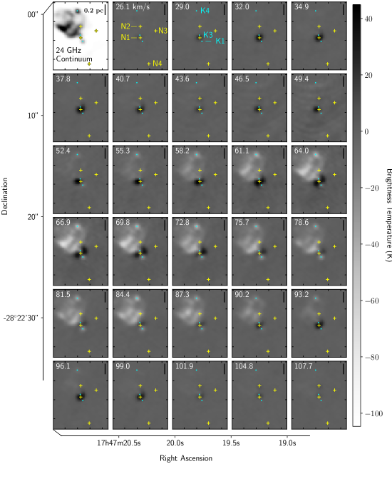
Figure 1.— Channel maps of emission from ¹⁴NH₃  (7,7) toward Sgr B2(N). The top left frame shows 24 GHz continuum emission, to illustrate the structure of the ionized gas in the region. The positions of the hot cores N1, N2, N3 and N4 are shown as yellow plus marks. The positions of the compact H II  regions K1, K3, and K4 are shown as cyan points. A 0.2 pc scale bar is plotted in the top right of each panel. In the ¹⁴NH₃  line the emission from N1 and N2 do not peak at their central velocities ( $\sim$63 and 73 km s^-1, respectively), but instead peak at velocities offset by $\pm$30km s^-1  from the central velocity, at the location of the optically-thinner hyperfine satellite lines. Widespread absorption is seen against continuum emission from the ‘K’ complex of compact and ultracompact H II  regions at velocities of $\sim$55-85 km s^-1. Semi-resolved absorption against the two compact H II  regions K1 and K3 is seen toward N1 at most of the velocities in this series of channel maps. The spatial resolution of these data is not sufficient to resolve the embedded hypercompact H II  regions K2 in N1 or K7 in N2, and thus no absorption against these features is detected.

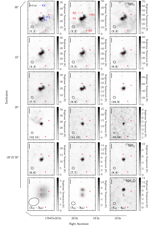
Figure 2.— Maps of the peak emission over all velocities from observed transitions of the NH₃  isotopologues ¹⁴NH₃, ¹⁵NH₃, and NH₂D  toward Sgr B2(N). The positions of the hot cores N1, N2, N3 and N4 are shown as red plus marks. The positions of the compact H II  regions K1, K3, and K4 are shown as blue points. All images shown in this figure are from the VLA observations except for the $2_{12}-2_{02}$ and $3_{13}-3_{03}$ lines of NH₂D, which are from observations with the ATCA. The beam size of each image is plotted in the bottom left corner, and exact spatial resolutions are given in Table 1. A 0.2 pc scale bar is plotted in the top left of each panel.

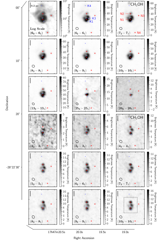
Figure 3.— Maps of peak emission over all velocities from the observed transitions of the CH₃OH  isotopologues CH₃OH  (top) and ¹³CH₃OH  (bottom) toward Sgr B2(N). The positions of the hot cores N1, N2, N3 and N4 are shown as red plus marks. The positions of the compact H II  regions K1, K3, and K4 are shown as blue points. The CH₃OH  ($6_{2}-6_{1}$) transition is plotted twice, first with a logarithmic scaling to highlight the fainter structure detected outside of the N1 and N2 cores. All images shown in this figure are from the VLA observations. The beam size of each image is plotted in the bottom left corner, and exact spatial resolutions are given in Table 1. A 0.2 pc scale bar is plotted in the top left of each panel. The rectangular region marked with dotted lines in the last panel indicates the area shown in Figures 4 and 7

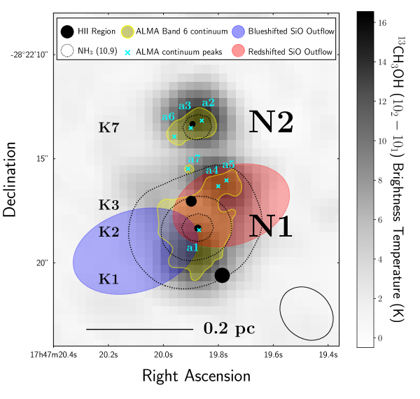
Figure 4.— A map of the currently identified components of Sgr B2(N). The background greyscale is the peak emission from ¹³CH₃OH  (10₂-10₁) from the VLA data. A 0.2 pc scale bar is plotted at the bottom. Dotted contours show the emission from the ¹⁴NH₃  (10,9) line in N2 and N1. The beam for both of these maps is displayed in the bottom right corner. The black circles represent the sizes and positions of compact H II  regions seen with the VLA at 8.4 GHz and 22 GHz by Gaume et al. (1995) and De Pree et al. (2015). The extent of the dust continuum emission from this region as seen in the Band 6 ALMA observations of Sánchez-Monge et al. (2017) is shown in yellow, as well as the seven strongest individual continuum peaks identified in that study, which are overplotted as cyan ‘x’s and numbered a1-a7. Also shown are the approximate positions of the red- and blue-shifted lobes of the outflow detected in SiO with ALMA by Higuchi et al. (2015)

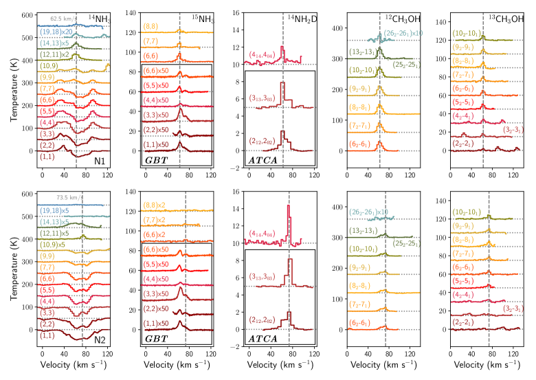
Figure 5.— Spectra of the observed transitions of NH₃, ¹⁵NH₃, NH₂D, CH₃OH, and ¹³CH₃OH  toward the two hot cores in Sgr B2(N): N1 (Top) and N2 (Bottom). From red to blue, colors correspond to transitions from low-$J$ to high-$J$ values. Spectra are from VLA observations unless otherwise indicated by a box showing spectra obtained from lower spatial-resolution observations with ATCA and the GBT. The GBT spectra for N1 and N2 are the same, as the observations are from a single pointing containing both sources that is centered on N1, with N2 at the 93% power position. The spatial and spectral resolutions of all of the data are given in Table 1.

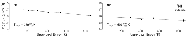
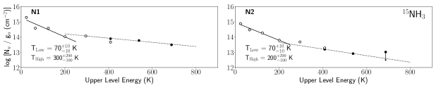
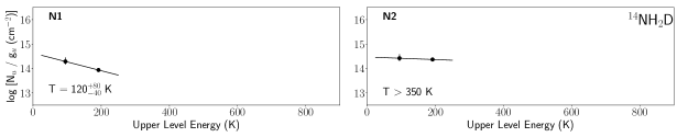
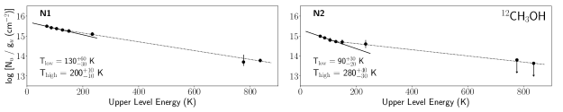
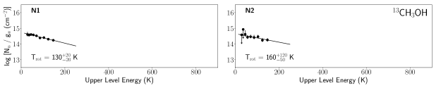
Figure 6.— Top to Bottom: Rotation temperature fits for non-metastable lines of ¹⁴NH₃, metastable lines of ¹⁴NH₃, ¹⁵NH₃, NH₂D, ¹²CH₃OH, and ¹³CH₃OH. All plots except those in the top row (non-metastable ¹⁴NH₃) are scaled to have an identical X-axis range and to have a Y-axis covering 4 orders of magnitude in column density, so that the temperature slopes derived for each molecule can be directly compared. For the ¹⁵NH₃  population diagram, GBT data are shown as open symbols and VLA data as filled symbols. For all NH₃  fits, the ortho to para ratio is fixed to be equal to its equilibrium value (2.0).

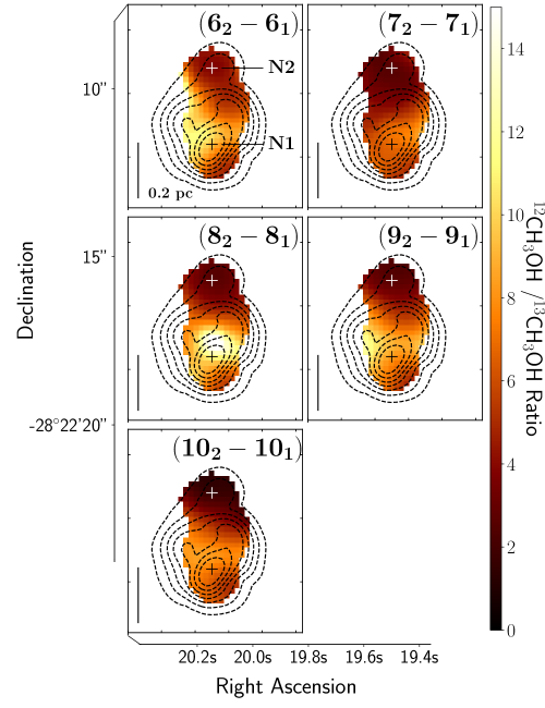
Figure 7.— Ratio maps for identical transitions of ¹²CH₃OH  and ¹³CH₃OH  with contours of CH₃OH  (10₂-10₁) overlaid. Maps are convolved to identical resolutions and pixelizations prior to taking the ratio. For optically-thin emission, the ratio should reflect the ¹²C/¹³C ratio of 25 in the Galactic center. Smaller values of this ratio correspond to large optical depths. A 0.2 pc scale bar is plotted in the bottom left of each panel.

Fitting of all spectral lines is accomplished using PySpecKit (Ginsburg & Mirocha, 2011), a python-based spectroscopic analysis toolkit for astronomy. As the combination of smoothed data and relatively large apertures leads to each pointing having some contribution from both N2 and N1, we fit each spectrum with two Gaussian components at the central velocities of N1 and N2. We then report the fit parameters of the Gaussian corresponding to the source (either N1 or N2) centered in the aperture from which the spectrum was extracted. For the (12,11) line of ¹⁴NH₃  toward N2, we fit for an additional component due to blending with the H63 $\alpha$ line. This component dominates the fitting, and leads to a larger uncertainty on the fitted line parameters. Fits are shown in Figures 8, 10, 11, 12, and 13 and the results of the fitting are reported in Tables 5 and 6. The reported errors on the peak and integrated brightness temperatures given in these tables originate both from the fitting errors and the uncertainty on the absolute flux calibration for each telescope (given in Section 2). These errors are added in quadrature, with the uncertainty due to the flux calibration typically dominating. Uncertainties on further derived quantities (e.g., column densities) are determined via propagation of these errors.

Unlike the other observed lines, the ¹⁴NH₃  line exhibits substantial absorption. However, this absorption is primarily confined to the central or main hyperfine component of the line. All of the hyperfine satellites in N1, and the J$\geq$4 hyperfine satellites in N2, appear in emission. We thus fit the hyperfine satellite lines in order to constrain the rotational temperature and column density of this molecule. We assume that the two hyperfine satellite components (with separations of $\sim$2-10 km s^-1, decreasing with increasing $J$) are blended, and fit them with a single Gaussian profile. For N1, we fit only the blueshifted (lower-velocity) satellite lines, as the redshifted satellite lines are subject to increased absorption. In contrast, for N2, the redshifted satellite lines appear more prominent, and we fit to just these lines (fits to the blueshifted satellite lines yield a lower column density, but a consistent rotational temperature). In general, above $J$=3 ($J$=4 for N2), the hyperfine satellites are well fit by a single Gaussian profile. The profiles of the J$<$4 lines in N1 are non-Gaussian, and appear to be affected by some combination of absorption from the main line and self-absorption in the satellite lines. The hyperfine satellites of the J$<5$ lines in N2 are not apparent, and are likely obscured by absorption. In Table 4 we report the line frequencies adopted for the blueshifted (N1) and redshifted (N2) blended hyperfine components. The velocities reported in Tables 5 and 6 are determined relative to these frequencies, and well match the expected source velocities of 64 km s^-1  for N1 and 73 km s^-1  for N2. Note that the velocity widths represent an average of the blended hyperfine components. While it is clear from the detection of the hyperfine satellites that the central line components are optically thick, we cannot measure the optical depth of individual hyperfine satellite lines (though as noted in Section 3.2.1, it seems likely that at least the lower-$J$ satellites are optically thick).

Table 4Adopted ¹⁴NH₃  Hyperfine Line Parameters

Transition	Blueshifted Hyperfines	Redshifted Hyperfines	Blended Main-to-Hyperfine
	Blended Frequency	Blended Frequency	Intensity Ratio
	(GHz)	(GHz)
(4,4)	24.141622		28.8
(5,5)	24.535328	24.530642	43.8
(6,6)	25.058470	25.053579	61.8
(7,7)	25.717706	25.712658	82.8
(9,9)	27.478247	27.477633	125

Table 5Measured Line Parameters and Column Densities

Species	Transition	vcen	vfwhm	Peak TMB	$\int T_{\mathrm{MB}}dv$	Nu	$g_{u}$	$f$
		(km s-1)	(km s-1)	(K)	(K km s-1)	( 1015 cm-2)
Source N1
14NH3	(4,4)	63.7 $\pm$ 0.1	19.9 $\pm$ 0.1	28.42 $\pm$ 2.85	602.3 $\pm$ 60.4	1216.6 $\pm$ 122.0	9	0.114
14NH3	(5,5)	64.3 $\pm$ 0.1	18.0 $\pm$ 0.1	27.07 $\pm$ 2.71	518.6 $\pm$ 51.9	1507.7 $\pm$ 150.9	11	0.114
14NH3	(6,6)	64.4 $\pm$ 0.1	18.0 $\pm$ 0.1	24.23 $\pm$ 2.42	464.2 $\pm$ 46.5	1817.3 $\pm$ 181.9	26	0.114
14NH3	(7,7)	63.8 $\pm$ 0.1	14.0 $\pm$ 0.1	14.62 $\pm$ 1.47	217.8 $\pm$ 21.9	1093.6 $\pm$ 109.9	15	0.114
14NH3	(9,9)	64.5 $\pm$ 0.2	13.0 $\pm$ 0.1	8.72 $\pm$ 0.89	120.6 $\pm$ 12.3	837.8 $\pm$ 85.7	38	0.114
14NH3	(10,9)	60.0 $\pm$ 0.1	10.0 $\pm$ 0.1	30.70 $\pm$ 3.21	326.8 $\pm$ 34.4	24.3 $\pm$ 2.6	38	0.114
14NH3	(12,11)	61.0 $\pm$ 0.2	10.0 $\pm$ 0.1	12.59 $\pm$ 1.32	134.0 $\pm$ 14.1	8.9 $\pm$ 0.9	23	0.114
14NH3	(14,13)	61.3 $\pm$ 0.5	8.7 $\pm$ 1.0	6.06 $\pm$ 0.68	56.1 $\pm$ 8.7	3.5 $\pm$ 0.5	27	0.114
14NH3	(19,18)	61.3 $\pm$ 1.9	9.5 $\pm$ 4.2	1.01 $\pm$ 0.24	10.2 $\pm$ 5.2	0.5 $\pm$ 0.2	74	0.114
15NH3	(1,1)	62.9 $\pm$ 0.1	9.4 $\pm$ 0.1	0.17 $\pm$ 0.02	1.7 $\pm$ 0.2	11.5 $\pm$ 1.2	3	0.0020
15NH3	(2,2)	62.2 $\pm$ 0.1	6.8 $\pm$ 0.1	0.10 $\pm$ 0.01	0.7 $\pm$ 0.1	3.8 $\pm$ 0.4	5	0.0020
15NH3	(3,3)	63.9 $\pm$ 0.1	8.7 $\pm$ 0.1	0.25 $\pm$ 0.03	2.3 $\pm$ 0.2	10.5 $\pm$ 1.0	14	0.0020
15NH3	(4,4)	63.5 $\pm$ 0.1	8.0 $\pm$ 0.1	0.05 $\pm$ 0.01	0.5 $\pm$ 0.0	1.9 $\pm$ 0.2	9	0.0020
15NH3	(5,5)	61.3 $\pm$ 0.1	5.9 $\pm$ 0.1	0.11 $\pm$ 0.01	0.7 $\pm$ 0.1	2.6 $\pm$ 0.3	11	0.0021
15NH3	(6,6)	62.5 $\pm$ 0.1	6.3 $\pm$ 0.1	0.10 $\pm$ 0.01	0.7 $\pm$ 0.1	2.4 $\pm$ 0.2	26	0.0022
15NH3	(6,6)	61.3 $\pm$ 0.1	6.7 $\pm$ 0.1	8.55 $\pm$ 0.86	61.0 $\pm$ 6.2	4.1 $\pm$ 0.4	26	0.114
15NH3	(7,7)	61.5 $\pm$ 0.1	4.8 $\pm$ 0.2	5.49 $\pm$ 0.57	28.0 $\pm$ 3.1	1.8 $\pm$ 0.2	15	0.114
15NH3	(8,8)	61.0 $\pm$ 0.1	5.4 $\pm$ 0.2	2.98 $\pm$ 0.31	17.3 $\pm$ 1.9	1.1 $\pm$ 0.1	17	0.114
14NH2D	313-303	61.9 $\pm$ 0.1	9.1 $\pm$ 0.2	2.52 $\pm$ 0.76	24.3 $\pm$ 7.3	8.2 $\pm$ 2.5	21	0.114
14NH2D	414-404	61.4 $\pm$ 0.2	5.1 $\pm$ 0.5	1.97 $\pm$ 0.24	10.7 $\pm$ 1.6	4.7 $\pm$ 0.7	27	0.114
12CH3OH	62-61	62.5 $\pm$ 0.1	9.9 $\pm$ 0.1	31.10 $\pm$ 3.12	327.7 $\pm$ 33.0	40.7 $\pm$ 4.1	13	0.114
12CH3OH	72-71	62.5 $\pm$ 0.1	9.7 $\pm$ 0.2	31.55 $\pm$ 3.17	325.9 $\pm$ 32.9	39.3 $\pm$ 4.0	15	0.114
12CH3OH	82-81	62.6 $\pm$ 0.1	10.0 $\pm$ 0.2	32.21 $\pm$ 3.24	341.5 $\pm$ 34.7	40.1 $\pm$ 4.1	17	0.114
12CH3OH	92-91	62.6 $\pm$ 0.1	9.8 $\pm$ 0.1	32.31 $\pm$ 3.23	337.5 $\pm$ 33.8	38.5 $\pm$ 3.9	19	0.114
12CH3OH	102-101	62.6 $\pm$ 0.1	9.6 $\pm$ 0.2	33.00 $\pm$ 3.32	337.3 $\pm$ 34.2	37.3 $\pm$ 3.8	21	0.114
12CH3OH	132-131	62.6 $\pm$ 0.1	8.5 $\pm$ 0.3	36.87 $\pm$ 3.76	333.6 $\pm$ 35.1	33.8 $\pm$ 3.6	27	0.114
12CH3OH	252-251	60.0 $\pm$ 0.1	4.7 $\pm$ 1.8	2.19 $\pm$ 0.80	10.9 $\pm$ 5.9	2.6 $\pm$ 1.4	51	0.114
12CH3OH	262-261	62.0 $\pm$ 0.2	4.0 $\pm$ 0.1	2.54 $\pm$ 0.33	10.8 $\pm$ 1.4	3.1 $\pm$ 0.4	53	0.114
13CH3OH	22-21	62.1 $\pm$ 0.6	5.1 $\pm$ 1.2	2.17 $\pm$ 0.47	11.9 $\pm$ 3.8	2.0 $\pm$ 0.6	5	0.114
13CH3OH	32-31	63.2 $\pm$ 0.4	5.1 $\pm$ 0.9	3.58 $\pm$ 0.61	19.4 $\pm$ 4.6	2.6 $\pm$ 0.6	7	0.114
13CH3OH	42-41	62.9 $\pm$ 0.3	6.0 $\pm$ 0.7	4.61 $\pm$ 0.60	29.3 $\pm$ 5.2	3.6 $\pm$ 0.6	9	0.114
13CH3OH	52-51	62.3 $\pm$ 0.2	6.2 $\pm$ 0.5	5.42 $\pm$ 0.63	35.5 $\pm$ 4.9	4.2 $\pm$ 0.6	11	0.114
13CH3OH	62-61	62.5 $\pm$ 0.3	6.3 $\pm$ 0.5	5.67 $\pm$ 0.64	37.9 $\pm$ 5.2	4.4 $\pm$ 0.6	13	0.114
13CH3OH	72-71	62.4 $\pm$ 0.2	5.7 $\pm$ 0.5	5.42 $\pm$ 0.65	32.8 $\pm$ 4.7	3.7 $\pm$ 0.5	15	0.114
13CH3OH	82-81	62.6 $\pm$ 0.3	6.1 $\pm$ 0.6	6.14 $\pm$ 0.78	40.0 $\pm$ 6.3	4.4 $\pm$ 0.7	17	0.114
13CH3OH	92-91	62.6 $\pm$ 0.3	6.3 $\pm$ 0.6	5.45 $\pm$ 0.67	36.5 $\pm$ 5.5	3.9 $\pm$ 0.6	19	0.114
13CH3OH	102-101	62.5 $\pm$ 0.2	5.9 $\pm$ 0.3	5.67 $\pm$ 0.61	35.3 $\pm$ 4.2	3.7 $\pm$ 0.4	21	0.114

Table 6Measured Line Parameters and Column Densities

Species	Transition	vcen	vfwhm	Peak TMB	$\int T_{\mathrm{MB}}dv$	Nu	$g_{u}$	$f$
		(km s-1)	(km s-1)	(K)	(K km s-1)	( 1014 cm-2)
Source N2
14NH3	(5,5)	72.8 $\pm$ 0.5	8.7 $\pm$ 1.0	3.14 $\pm$ 0.43	29.2 $\pm$ 5.3	1271.6 $\pm$ 229.1	11	0.076
14NH3	(6,6)	73.1 $\pm$ 0.5	8.8 $\pm$ 1.0	2.98 $\pm$ 0.41	27.9 $\pm$ 5.1	1638.0 $\pm$ 299.2	26	0.076
14NH3	(7,7)	73.3 $\pm$ 0.9	8.9 $\pm$ 2.0	2.07 $\pm$ 0.45	19.6 $\pm$ 6.3	1473.0 $\pm$ 474.5	15	0.076
14NH3	(9,9)	74.4 $\pm$ 1.1	7.6 $\pm$ 2.4	1.77 $\pm$ 0.51	14.4 $\pm$ 6.3	1497.8 $\pm$ 660.6	38	0.076
14NH3	(10,9)	74.2 $\pm$ 0.4	7.7 $\pm$ 0.9	3.20 $\pm$ 0.42	26.3 $\pm$ 4.7	2.9 $\pm$ 0.5	38	0.076
14NH3	(12,11)	72.8 $\pm$ 0.7	5.7 $\pm$ 1.8	0.83 $\pm$ 0.23	5.1 $\pm$ 2.1	0.5 $\pm$ 0.2	23	0.076
14NH3	(14,13)			$<$ 0.25	$<$ 2.2	$<$ 0.1	27	0.076
14NH3	(19,18)			$<$ 0.60	$<$ 2.5	$<$ 0.1	74	0.076
15NH3	(1,1)	72.9 $\pm$ 0.1	6.9 $\pm$ 0.1	0.06 $\pm$ 0.01	0.4 $\pm$ 0.0	42.0 $\pm$ 4.2	3	0.0013
15NH3	(2,2)	73.1 $\pm$ 0.1	7.1 $\pm$ 0.1	0.05 $\pm$ 0.00	0.4 $\pm$ 0.0	27.5 $\pm$ 2.7	5	0.0013
15NH3	(3,3)	74.2 $\pm$ 0.1	7.1 $\pm$ 0.1	0.09 $\pm$ 0.01	0.7 $\pm$ 0.1	48.4 $\pm$ 4.8	14	0.0013
15NH3	(4,4)	74.1 $\pm$ 0.1	7.2 $\pm$ 0.1	0.02 $\pm$ 0.00	0.2 $\pm$ 0.0	10.3 $\pm$ 1.0	9	0.0014
15NH3	(5,5)	72.4 $\pm$ 0.1	5.0 $\pm$ 0.1	0.03 $\pm$ 0.00	0.2 $\pm$ 0.0	9.8 $\pm$ 1.0	11	0.0014
15NH3	(6,6)	73.5 $\pm$ 0.1	5.0 $\pm$ 0.1	0.03 $\pm$ 0.00	0.2 $\pm$ 0.0	9.3 $\pm$ 0.9	26	0.0015
15NH3	(6,6)	73.5 $\pm$ 0.7	6.8 $\pm$ 1.6	1.13 $\pm$ 0.23	8.2 $\pm$ 2.6	8.2 $\pm$ 2.6	26	0.076
15NH3	(7,7)	72.6 $\pm$ 0.9	4.1 $\pm$ 1.6	0.59 $\pm$ 0.19	2.6 $\pm$ 1.3	2.5 $\pm$ 1.3	15	0.076
15NH3	(8,8)			$<$ 0.52	$<$ 2.2	$<$ 3.5	17	0.076
14NH2D	313-303	74.7 $\pm$ 0.1	10.1 $\pm$ 0.2	2.05 $\pm$ 0.62	22.0 $\pm$ 6.6	111.1 $\pm$ 33.4	21	0.076
14NH2D	414-404	73.5 $\pm$ 0.2	4.7 $\pm$ 0.4	3.86 $\pm$ 0.43	19.2 $\pm$ 2.5	126.9 $\pm$ 16.8	27	0.076
12CH3OH	62-61	72.9 $\pm$ 0.2	6.1 $\pm$ 0.4	10.53 $\pm$ 1.14	68.7 $\pm$ 8.3	128.0 $\pm$ 15.5	13	0.076
12CH3OH	72-71	73.1 $\pm$ 0.2	6.2 $\pm$ 0.3	10.28 $\pm$ 1.10	67.4 $\pm$ 8.1	122.0 $\pm$ 14.7	15	0.076
12CH3OH	82-81	73.0 $\pm$ 0.4	6.0 $\pm$ 0.6	9.47 $\pm$ 1.18	60.8 $\pm$ 14.1	107.0 $\pm$ 24.8	17	0.076
12CH3OH	92-91	73.0 $\pm$ 0.1	6.0 $\pm$ 0.2	9.23 $\pm$ 0.94	59.0 $\pm$ 6.8	101.0 $\pm$ 11.6	19	0.076
12CH3OH	102-101	72.8 $\pm$ 0.4	6.6 $\pm$ 0.9	9.06 $\pm$ 1.12	63.6 $\pm$ 19.2	105.6 $\pm$ 31.9	21	0.076
12CH3OH	132-131	72.8 $\pm$ 0.7	6.2 $\pm$ 1.4	10.87 $\pm$ 1.77	71.2 $\pm$ 38.9	108.2 $\pm$ 59.2	27	0.076
12CH3OH	252-251			$<$ 0.65	$<$ 3.1	$<$ 10.9	51	0.076
12CH3OH	262-261			$<$ 0.41	$<$ 1.8	$<$ 7.6	53	0.076
13CH3OH	22-21			$<$ 1.02	$<$ 7.6	$<$ 19.3	5	0.076
13CH3OH	32-31			$<$ 3.96	$<$ 44.7	$<$ 59.8	7	0.076
13CH3OH	42-41	72.9 $\pm$ 1.0	7.1 $\pm$ 2.3	2.67 $\pm$ 0.79	20.2 $\pm$ 8.9	37.7 $\pm$ 16.5	9	0.076
13CH3OH	52-51	73.1 $\pm$ 0.5	5.0 $\pm$ 1.0	3.13 $\pm$ 0.59	16.7 $\pm$ 4.6	29.7 $\pm$ 8.2	11	0.076
13CH3OH	62-61	73.3 $\pm$ 0.5	5.2 $\pm$ 1.0	3.94 $\pm$ 0.72	22.0 $\pm$ 5.9	37.9 $\pm$ 10.1	13	0.076
13CH3OH	72-71	73.4 $\pm$ 0.7	6.8 $\pm$ 1.5	3.23 $\pm$ 0.69	23.5 $\pm$ 7.4	39.4 $\pm$ 12.4	15	0.076
13CH3OH	82-81	73.4 $\pm$ 0.5	6.0 $\pm$ 1.0	4.81 $\pm$ 0.77	30.7 $\pm$ 7.1	50.1 $\pm$ 11.5	17	0.076
13CH3OH	92-91	73.1 $\pm$ 0.5	5.1 $\pm$ 1.1	3.84 $\pm$ 0.76	20.7 $\pm$ 6.0	33.0 $\pm$ 9.6	19	0.076
13CH3OH	102-101	73.5 $\pm$ 0.4	5.1 $\pm$ 1.0	4.51 $\pm$ 0.69	24.6 $\pm$ 6.1	38.1 $\pm$ 9.5	21	0.076

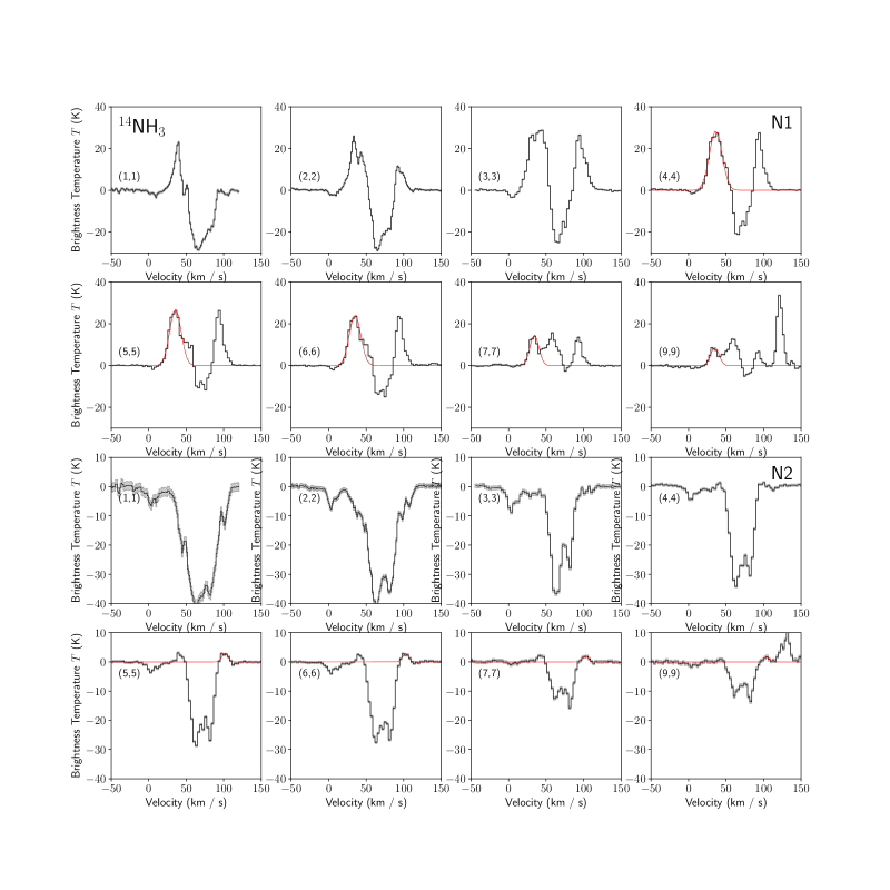
Figure 8.— Fitted spectra of ¹⁴NH₃  metastable transitions. Where possible ($J>4$ for the N2 source) a single Gaussian is fit to the blended hyperfine satellite lines that appear in emission. Red curves show Gaussian fits to each line. For N1 (v=63.5 km s^-1) fits are performed for the blueshifted satellite lines, as these are subject to less absorption. For N2 (v=73 km s^-1), fits are performed for the redshifted satellite lines, for the same reason.

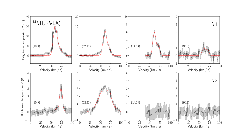
Figure 9.— Fitted spectra of ¹⁴NH₃  nonmetastable transitions. For each line, two Gaussian components are fit, for the contribution from the N1 source at 63.5 km s^-1  and the N2 source at 73 km s^-1. The (12,11) line toward N2 is dominated by contamination from the H63$\alpha$ line, tracing ionized gas in the H II  regions along the line of sight.

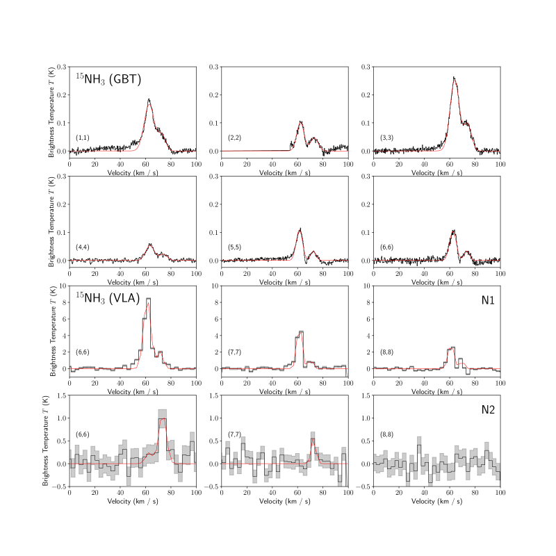
Figure 10.— Fitted spectra of ¹⁵NH₃  metastable transitions. Spectra from GBT and VLA observations are labeled. For each line, two Gaussian components are fit, for the contribution from the N1 source at 63.5 km s^-1  and the N2 source at 73 km s^-1.

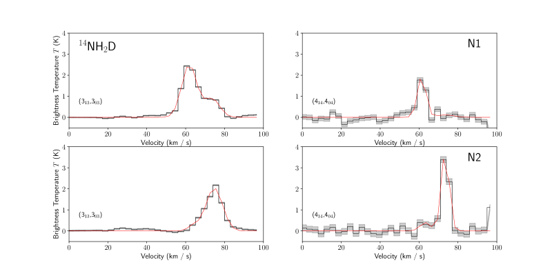
Figure 11.— Fitted spectra of NH₂D  transitions. The $3_{13}-3_{03}$ transition is from ATCA observations, while the $4_{14}-4_{04}$ transition is from VLA observations. For each line, two Gaussian components are fit, for the contribution from the N1 source at 63.5 km s^-1  and the N2 source at 73 km s^-1.

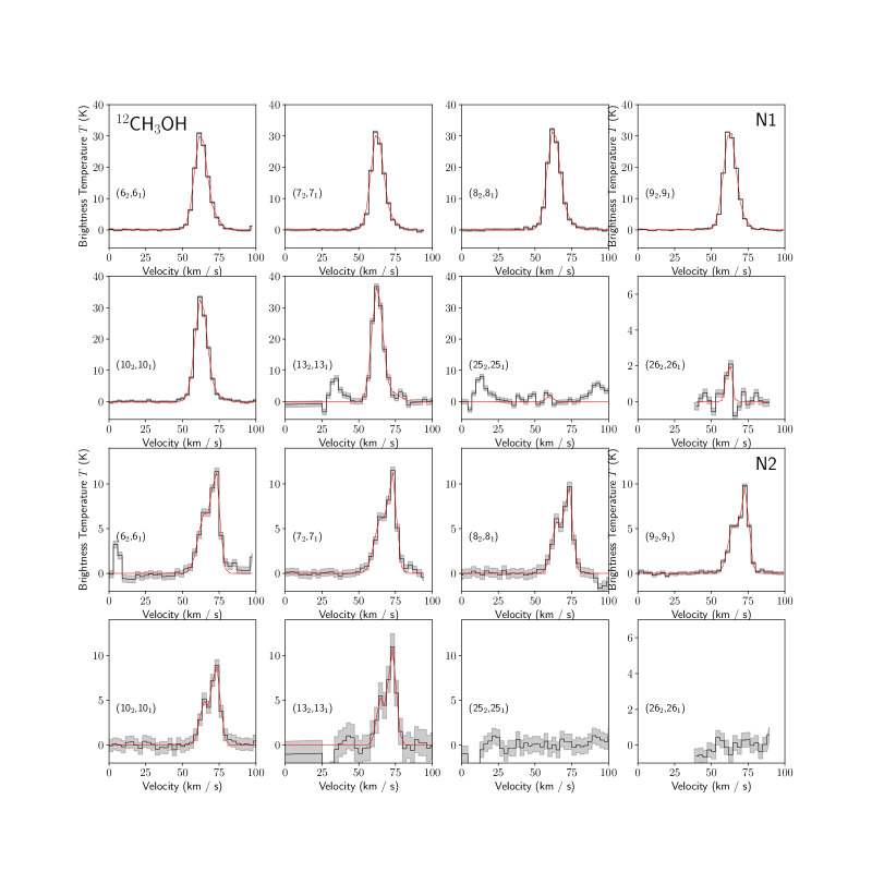
Figure 12.— Fitted spectra of ¹²CH₃OH  transitions. The $25_{2}-25_{1}$ transition is fit after subtracting the nearby and much stronger $13_{2}-13_{1}$ line from the spectrum. For each line, two Gaussian components are fit, for the contribution from the N1 source at 63.5 km s^-1  and the N2 source at 73 km s^-1.

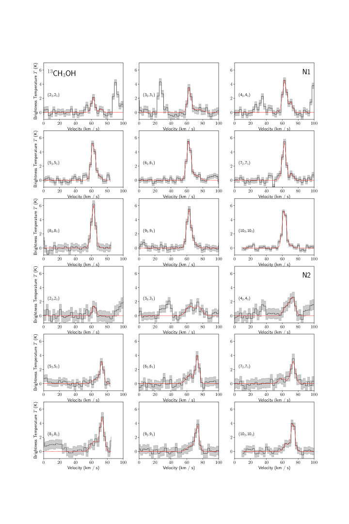
Figure 13.— Fitted spectra of ¹³CH₃OH  transitions. Note that the $2_{2}-2_{1}$, $4_{2}-4_{1}$ and $3_{2}-3_{1}$ lines are closely spaced, and each can be seen in the spectra of the other two lines. For each line, two Gaussian components are fit, for the contribution from the N1 source at 63.5 km s^-1  and the N2 source at 73 km s^-1.

References

- Adams (2010) Adams, F. C. 2010, ARA&A, 48, 47
- Adande & Ziurys (2011) Adande, G. R., & Ziurys, L. M. 2011, ApJ, 744, 194
- Aléon (2010) Aléon, J. 2010, ApJ, 722, 1342
- Ao et al. (2013) Ao, Y., Henkel, C., Menten, K. M., et al. 2013, A&A, 550, A135
- Arpigny et al. (2003) Arpigny, C., Jehin, E., Manfroid, J., et al. 2003, Science, 301, 1522
- Belloche et al. (2013) Belloche, A., M ller, H. S. P., Menten, K. M., Schilke, P., & Comito, C. 2013, A&A, 559, A47
- Belloche et al. (2008) Belloche, A., Menten, K. M., Comito, C., et al. 2008, A&A, 482, 179
- Belloche et al. (2016) Belloche, A., Müller, H. S. P., Garrod, R. T., & Menten, K. M. 2016, A&A, 587, A91
- Blake et al. (1987) Blake, G. A., Sutton, E. C., Masson, C. R., & Phillips, T. G. 1987, ApJ, 315, 621
- Bockelée-Morvan et al. (2008) Bockelée-Morvan, D., Biver, N., Jehin, E., et al. 2008, ApJ, 679, L49
- Boehle et al. (2016) Boehle, A., Ghez, A. M., Schödel, R., et al. 2016, ApJ, 830, 1
- Bøgelund et al. (2018) Bøgelund, E. G., McGuire, B. A., Ligterink, N. F. W., et al. 2018, A&A, 615, A88
- Bonal et al. (2010) Bonal, L., Huss, G. R., Krot, A. N., et al. 2010, Geochim. Cosmochim. Acta, 74, 6590
- Bonfand et al. (2017) Bonfand, M., Belloche, A., Menten, K. M., Garrod, R. T., & Müller, H. S. P. 2017, A&A, 604, A60
- Bouhafs et al. (2017) Bouhafs, N., Rist, C., Daniel, F., et al. 2017, MNRAS, 470, 2204
- Briani et al. (2009) Briani, G., Gounelle, M., Marrocchi, Y., et al. 2009, Proceedings of the National Academy of Science, 106, 10522
- Brown & Millar (1989) Brown, P. D., & Millar, T. J. 1989, MNRAS, 240, 25P
- Busemann et al. (2006) Busemann, H., Young, A. F., O’D. Alexander, C. M., et al. 2006, Science, 312, 727
- Busquet et al. (2010) Busquet, G., Palau, A., Estalella, R., et al. 2010, A&A, 517, L6
- Butterfield et al. (2018) Butterfield, N., Lang, C. C., Morris, M., Mills, E. A. C., & Ott, J. 2018, ApJ, 852, 11
- Cazaux et al. (2011) Cazaux, S., Caselli, P., & Spaans, M. 2011, ApJ, 741, L34
- Ceccarelli et al. (2002) Ceccarelli, C., Baluteau, J. P., Walmsley, M., et al. 2002, A&A, 383, 603
- Clark et al. (2013) Clark, P. C., Glover, S. C. O., Ragan, S. E., Shetty, R., & Klessen, R. S. 2013, ApJ, 768, L34
- Collings et al. (2004) Collings, M. P., Anderson, M. A., Chen, R., et al. 2004, MNRAS, 354, 1133
- Corby et al. (2015) Corby, J. F., Jones, P. A., Cunningham, M. R., et al. 2015, MNRAS, 452, 3969
- Danby et al. (1988) Danby, G., Flower, D. R., Valiron, P., Schilke, P., & Walmsley, C. M. 1988, MNRAS, 235, 229
- De Pree et al. (1998) De Pree, C. G., Goss, W. M., & Gaume, R. A. 1998, ApJ, 500, 847
- De Pree et al. (2015) De Pree, C. G., Peters, T., Mac Low, M. M., et al. 2015, ApJ, 815, 123
- De Simone et al. (2018) De Simone, M., Fontani, F., Codella, C., et al. 2018, MNRAS, 476, 1982
- de Vicente et al. (2000) de Vicente, P., Martín-Pintado, J., Neri, R., & Colom, P. 2000, A&A, 361, 1058
- Dukes & Krumholz (2012) Dukes, D., & Krumholz, M. R. 2012, ApJ, 754, 56
- Etxaluze et al. (2011) Etxaluze, M., Smith, H. A., Tolls, V., Stark, A. A., & González-Alfonso, E. 2011, AJ, 142, 134
- Etxaluze et al. (2013) Etxaluze, M., Goicoechea, J. R., Cernicharo, J., et al. 2013, A&A, 556, A137
- Floss et al. (2006) Floss, C., Stadermann, F. J., Bradley, J. P., et al. 2006, Geochim. Cosmochim. Acta, 70, 2371
- Flower et al. (1995) Flower, D. R., Pineau des Forets, G., & Walmsley, C. M. 1995, A&A, 294, 815
- Fontani et al. (2015a) Fontani, F., Busquet, G., Palau, A., et al. 2015a, A&A, 575, A87
- Fontani et al. (2015b) Fontani, F., Caselli, P., Palau, A., Bizzocchi, L., & Ceccarelli, C. 2015b, ApJ, 808, L46
- Fouchet et al. (2004) Fouchet, T., Irwin, P. G. J., Parrish, P., et al. 2004, Icarus, 172, 50
- Gaume et al. (1995) Gaume, R. A., Claussen, M. J., de Pree, C. G., Goss, W. M., & Mehringer, D. M. 1995, ApJ, 449, 663
- Genzel et al. (1982) Genzel, R., Ho, P. T. P., Bieging, J., & Downes, D. 1982, ApJ, 259, L103
- Ginsburg & Mirocha (2011) Ginsburg, A., & Mirocha, J. 2011, PySpecKit: Python Spectroscopic Toolkit, Astrophysics Source Code Library, ascl:1109.001
- Ginsburg et al. (2016) Ginsburg, A., Henkel, C., Ao, Y., et al. 2016, A&A, 586, A50
- Ginsburg et al. (2017) Ginsburg, A., Goddi, C., Kruijssen, J. M. D., et al. 2017, ApJ, 842, 92
- Goldsmith & Langer (1999) Goldsmith, P. F., & Langer, W. D. 1999, ApJ, 517, 209
- González-Alfonso et al. (2013) González-Alfonso, E., Fischer, J., Bruderer, S., et al. 2013, A&A, 550, A25
- Gordon et al. (1993) Gordon, M. A., Berkermann, U., Mezger, P. G., et al. 1993, A&A, 280, 208
- Gravity Collaboration et al. (2018) Gravity Collaboration, Abuter, R., Amorim, A., et al. 2018, A&A, 615, L15
- Guzmán et al. (2015) Guzmán, A. E., Sanhueza, P., Contreras, Y., et al. 2015, ApJ, 815, 130
- Guzmán et al. (2017) Guzmán, V. V., Öberg, K. I., Huang, J., Loomis, R., & Qi, C. 2017, ApJ, 836, 30
- Hacar et al. (2016) Hacar, A., Alves, J., Burkert, A., & Goldsmith, P. 2016, A&A, 591, A104
- Halfen et al. (2017) Halfen, D. T., Woolf, N. J., & Ziurys, L. M. 2017, ApJ, 845, 158
- Hasegawa et al. (1994) Hasegawa, T., Sato, F., Whiteoak, J. B., & Miyawaki, R. 1994, ApJ, 429, L77
- Hatchell (2003) Hatchell, J. 2003, A&A, 403, L25
- Herzberg & Crawford (1946) Herzberg, G., & Crawford, B. L. 1946, The Journal of Physical Chemistry, 50, 288
- Higuchi et al. (2015) Higuchi, A. E., Hasegawa, T., Saigo, K., Sanhueza, P., & Chibueze, J. O. 2015, ApJ, 815, 1
- Hoffman et al. (1979) Hoffman, J. H., Hodges, R. R., McElroy, M. B., Donahue, T. M., & Kolpin, M. 1979, Science, 205, 49
- Hollis et al. (2003) Hollis, J. M., Pedelty, J. A., Boboltz, D. A., et al. 2003, ApJ, 596, L235
- Huettemeister et al. (1995) Huettemeister, S., Wilson, T. L., Mauersberger, R., et al. 1995, A&A, 294, 667
- Hüttemeister et al. (1993) Hüttemeister, S., Wilson, T. L., Henkel, C., & Mauersberger, R. 1993, A&A, 276, 445
- Jacq et al. (1999) Jacq, T., Baudry, A., Walmsley, C. M., & Caselli, P. 1999, A&A, 347, 957
- Jacq et al. (1990) Jacq, T., Walmsley, C. M., & Henkel, C. 1990, A&A, 228
- Junk & Svec (1958) Junk, G., & Svec, H. J. 1958, Geochim. Cosmochim. Acta, 14, 234
- Kaifu et al. (1975) Kaifu, N., Morris, M., Palmer, P., & Zuckerman, B. 1975, ApJ, 201, 98
- Kauffmann et al. (2008) Kauffmann, J., Bertoldi, F., Bourke, T. L., Evans, II, N. J., & Lee, C. W. 2008, A&A, 487, 993
- Krieger et al. (2017) Krieger, N., Ott, J., Beuther, H., et al. 2017, ApJ, 850, 77
- Lis & Goldsmith (1989) Lis, D. C., & Goldsmith, P. F. 1989, ApJ, 337, 704
- Lis & Goldsmith (1991) Lis, D. C., & Goldsmith, P. F. 1991, ApJ, 369, 157
- Lis et al. (1993) Lis, D. C., Goldsmith, P. F., Carlstrom, J. E., & Scoville, N. Z. 1993, ApJ, 402, 238
- Lis et al. (1990) Lis, D. C., Goldsmith, P. F., Hills, R., & Lasenby, J. 1990, in Astrophysics and Space Science Library, Vol. 158, Submillimetre Astronomy, ed. G. D. Watt & A. S. Webster, 183–184
- Lis et al. (2010) Lis, D. C., Wootten, A., Gerin, M., & Roueff, E. 2010, ApJ, 710, L49
- Lis et al. (2014) Lis, D. C., Schilke, P., Bergin, E. A., et al. 2014, ApJ, 785, 135
- Longmore et al. (2012) Longmore, S. N., Rathborne, J., Bastian, N., et al. 2012, ApJ, 746, 117
- Loomis et al. (2013) Loomis, R. A., Zaleski, D. P., Steber, A. L., et al. 2013, ApJ, 765, L9
- Ludovici et al. (2016) Ludovici, D. A., Lang, C. C., Morris, M. R., et al. 2016, ApJ, 826, 218
- Manfroid et al. (2009) Manfroid, J., Jehin, E., Hutsemékers, D., et al. 2009, A&A, 503, 613
- Maret et al. (2009) Maret, S., Faure, A., Scifoni, E., & Wiesenfeld, L. 2009, MNRAS, 399, 425
- Marty et al. (2010) Marty, B., Zimmermann, L., Burnard, P. G., et al. 2010, Geochim. Cosmochim. Acta, 74, 340
- Mehringer et al. (1994) Mehringer, D. M., Goss, W. M., & Palmer, P. 1994, ApJ, 434, 237
- Mehringer & Menten (1997) Mehringer, D. M., & Menten, K. M. 1997, ApJ, 474, 346
- Meibom et al. (2007) Meibom, A., Krot, A. N., Robert, F., et al. 2007, ApJ, 656, L33
- Menten et al. (1986) Menten, K. M., Walmsley, C. M., Henkel, C., & Wilson, T. L. 1986, A&A, 157, 318
- Messenger (2000) Messenger, S. 2000, Nature, 404, 968
- Miao et al. (1995) Miao, Y., Mehringer, D. M., Kuan, Y.-J., & Snyder, L. E. 1995, ApJ, 445, L59
- Mills et al. (2015) Mills, E. A. C., Butterfield, N., Ludovici, D. A., et al. 2015, ApJ, 805, 72
- Mills et al. (2014) Mills, E. A. C., Lang, C. C., Morris, M. R., et al. 2014, in IAU Symposium, Vol. 303, IAU Symposium, ed. L. O. Sjouwerman, C. C. Lang, & J. Ott, 139–143
- Mills & Morris (2013) Mills, E. A. C., & Morris, M. R. 2013, ApJ, 772, 105
- Molinari et al. (2011) Molinari, S., Bally, J., Noriega-Crespo, A., et al. 2011, ApJ, 735, L33
- Morris et al. (1983) Morris, M., Polish, N., Zuckerman, B., & Kaifu, N. 1983, AJ, 88, 1228
- Morris et al. (1976) Morris, M., Turner, B. E., Palmer, P., & Zuckerman, B. 1976, ApJ, 205, 82
- Müller et al. (2005) Müller, H. S. P., Schlöder, F., Stutzki, J., & Winnewisser, G. 2005, Journal of Molecular Structure, 742, 215
- Müller et al. (2001) Müller, H. S. P., Thorwirth, S., Roth, D. A., & Winnewisser, G. 2001, A&A, 370, L49
- Müller et al. (2016) Müller, H. S. P., Belloche, A., Xu, L.-H., et al. 2016, A&A, 587, A92
- Neill et al. (2012) Neill, J. L., Muckle, M. T., Zaleski, D. P., et al. 2012, ApJ, 755, 153
- Nummelin et al. (2000) Nummelin, A., Bergman, P., Hjalmarson, Å., et al. 2000, ApJS, 128, 213
- Oka et al. (1971) Oka, T., Shimizu, F. O., Shimizu, T., & Watson, J. K. G. 1971, AJ, 165, L15
- Owen et al. (2001) Owen, T., Mahaffy, P. R., Niemann, H. B., Atreya, S., & Wong, M. 2001, ApJ, 553, L77
- Parise et al. (2006) Parise, B., Ceccarelli, C., Tielens, A. G. G. M., et al. 2006, A&A, 453, 949
- Pauls et al. (1983) Pauls, A., Wilson, T. L., Bieging, J. H., & Martin, R. N. 1983, A&A, 124, 23
- Pei et al. (2000) Pei, C. C., Liu, S.-Y., & Snyder, L. E. 2000, ApJ, 530, 800
- Peng et al. (1993) Peng, Y., Vogel, S. N., & Carlstrom, J. E. 1993, ApJ, 418, 255
- Pfalzner (2013) Pfalzner, S. 2013, A&A, 549, A82
- Phillips et al. (1979) Phillips, T. G., Huggins, P. J., Wannier, P. G., & Scoville, N. Z. 1979, ApJ, 231, 720
- Pickett et al. (1998) Pickett, H. M., Poynter, R. L., Cohen, E. A., et al. 1998, J. Quant. Spec. Radiat. Transf., 60, 883
- Qin et al. (2011) Qin, S.-L., Schilke, P., Rolffs, R., et al. 2011, A&A, 530, L9
- Reid et al. (2009) Reid, M. J., Menten, K. M., Zheng, X. W., Brunthaler, A., & Xu, Y. 2009, ApJ, 705, 1548
- Reid et al. (1988) Reid, M. J., Schneps, M. H., Moran, J. M., et al. 1988, ApJ, 330, 809
- Riquelme et al. (2010) Riquelme, D., Amo-Baladrón, M. A., Martín-Pintado, J., et al. 2010, A&A, 523, A51
- Rodgers & Charnley (2008) Rodgers, S. D., & Charnley, S. B. 2008, MNRAS, 385, L48
- Rodgers & Millar (1996) Rodgers, S. D., & Millar, T. J. 1996, MNRAS, 280, 1046
- Sánchez-Monge et al. (2017) Sánchez-Monge, Á., Schilke, P., Schmiedeke, A., et al. 2017, A&A, 604, A6
- Schmiedeke et al. (2016) Schmiedeke, A., Schilke, P., Möller, T., et al. 2016, A&A, 588, A143
- Scoville et al. (1975a) Scoville, N. Z., Solomon, P. M., & Penzias, A. A. 1975a, ApJ, 201, 352
- Scoville et al. (1975b) —. 1975b, ApJ, 201, 352
- Shah & Wootten (2001) Shah, R. Y., & Wootten, A. 2001, ApJ, 554, 933
- Snyder et al. (1994) Snyder, L. E., Kuan, Y. J., & Miao, Y. 1994, The Structure and Content of Molecular Clouds, 439, 187
- Sweitzer et al. (1979) Sweitzer, J. S., Palmer, P., Morris, M., Turner, B. E., & Zuckerman, B. 1979, ApJ, 227, 415
- Taquet et al. (2012) Taquet, V., Ceccarelli, C., & Kahane, C. 2012, ApJ, 748, L3
- Visser et al. (2018) Visser, R., Bruderer, S., Cazzoletti, P., et al. 2018, A&A, 615, A75
- Viti & Williams (1999) Viti, S., & Williams, D. A. 1999, MNRAS, 305, 755
- Vogel et al. (1987) Vogel, S. N., Genzel, R., & Palmer, P. 1987, ApJ, 316, 243
- Walker et al. (2016) Walker, D. L., Longmore, S. N., Bastian, N., et al. 2016, MNRAS, 457, 4536
- Walmsley et al. (1987) Walmsley, C. M., Hermsen, W., Henkel, C., Mauersberger, R., & Wilson, T. L. 1987, A&A, 172, 311
- Wannier et al. (1981) Wannier, P. G., Linke, R. A., & Penzias, A. A. 1981, ApJ, 247, 522
- Wilson et al. (2006) Wilson, T. L., Henkel, C., & Hüttemeister, S. 2006, A&A, 460, 533
- Wilson & Rood (1994) Wilson, T. L., & Rood, R. 1994, ARA&A, 32, 191
- Wilson et al. (2011) Wilson, W. E., Ferris, R. H., Axtens, P., et al. 2011, MNRAS, 416, 832
- Wirström et al. (2012) Wirström, E. S., Charnley, S. B., Cordiner, M. A., & Milam, S. N. 2012, ApJ, 757, L11
- Xu & Lovas (1997) Xu, L.-H., & Lovas, F. J. 1997, Journal of Physical and Chemical Reference Data, 26, 17
- Zaleski et al. (2013) Zaleski, D. P., Seifert, N. A., Steber, A. L., et al. 2013, ApJ, 765, L10
- Zhao & Wright (2011) Zhao, J.-H., & Wright, M. C. H. 2011, ApJ, 742, 50