CLEASE: A versatile and user-friendly implementation of Cluster Expansion method
Abstract
Materials exhibiting a substitutional disorder such as multicomponent alloys and mixed metal oxides/oxyfluorides are of great importance in many scientific and technological sectors. Disordered materials constitute an overwhelmingly large configurational space, which makes it practically impossible to be explored manually using first-principles calculations such as density functional theory (DFT) due to the high computational costs. Consequently, the use of methods such as cluster expansion (CE) is vital in enhancing our understanding of the disordered materials. CE dramatically reduces the computational cost by mapping the first-principles calculation results on to a Hamiltonian which is much faster to evaluate. In this work, we present our implementation of the CE method, which is integrated as a part of the Atomic Simulation Environment (ASE) open-source package. The versatile and user-friendly code automates the complex set up and construction procedure of CE while giving the users the flexibility to tweak the settings and to import their own structures and previous calculation results. Recent advancements such as regularization techniques from machine learning are implemented in the developed code. The code allows the users to construct CE on any bulk lattice structure, which makes it useful for a wide range of applications involving complex materials. We demonstrate the capabilities of our implementation by analyzing the two example materials with varying complexities: a binary metal alloy and a disordered lithium chromium oxyfluoride.
I Introduction
Computational modeling of materials with a substitutional disorder such as multicomponent alloys and mixed metal oxides is said to have a configurational problem. The vast configurational space of these materials makes it practically impossible to explore directly using first-principles calculations such as density functional theory (DFT). A quantitative method capable of establishing the relationship between the structure and property of materials is therefore essential. Cluster Expansion (CE) Sanchez, Ducastelle, and Gratias (1984); Fontaine (1994); Zunger (1994); Asta, Ozolins, and Woodward (2001); van de Walle (2008); Zhang and Sluiter (2016) is a method that has been used successfully in the past few decades to parameterize and express the configurational dependence of physical properties. The most widely parameterized physical property is energy computed using first-principles methods, but CE can also be used to parameterize other quantities such as band gap Magri and Zunger (1991); Franceschetti and Zunger (1999) and density of states Geng, Sluiter, and Chen (2005).
Despite its success and usefulness in predicting physical properties of crystalline materials, CE remains as a niche tool used in a small subfield within the computational materials science, primarily used by specialists. On the other hand, the research fields in which CE is becoming relevant is on the rise; one such example is the use of disordered materials for battery applications Wang et al. (2015); Abdellahi et al. (2016a, b); Urban et al. (2016); Kitchaev et al. (2018). The objective of our work is to make cluster expansion more accessible for a broad range of computational scientists who do not necessarily possess expertise in cluster expansion. Our approach to achieving such a goal is to implement CE as a part of a widely used, open-source Atomic Simulation Environment (ASE) package Hjorth Larsen et al. (2017). Henceforth, we refer to our implementation as CLEASE, which stands for CLuster Expansion in Atomic Simulation Environment.
Having CE as a part of a widely used package with interfaces to a multitude of open-source and commercial atomic-scale simulation codes accompanies several practical benefits: (1) a large existing user base does not need to install or learn a new program as the CE module is a part of ASE and inherits its syntax and code style, and (2) all of the atomic-scale simulation codes supported by ASE are also automatically supported by the implemented module. In addition, CLEASE utilizes the database management feature implemented in ASE, which provides an efficient way to store, maintain and share both DFT and CE results. Therefore, the implementation presented in this article appeals to a significant portion of computational materials science community as a versatile and easy-to-learn package, thereby lowering the barrier to incorporate cluster expansion as a part of their research methods to accelerate computational materials prediction and design.
The rest of the paper is organized as follows. A brief overview of cluster expansion formalism and other important concepts are provided in section II in order to aid the readers who are not familiar with the cluster expansion method. The implementation of CLEASE is described in section III. Section IV contains two application examples with different levels of complexities, namely a binary metal alloy and a lithium metal oxyfluoride. The computational settings and technical details for the examples are provided in section V.
II Theory
II.1 Cluster Expansion Formalism
The core concept of the cluster expansion is to express the scalar physical quantity of a material, , to its configuration, , where a crystalline system is represented with a fixed underlying grid of atomic sites. In such a representation, any configuration with the same underlying topology can be completely specified by the atomic occupation of each atomic site. For the case of a crystalline material with atomic sites, any configuration can be specified by an -dimensional vector , where is a site variable that specifies which type of atom occupies the atomic site (also referred to as an occupation variable Zarkevich and Johnson (2004); Meng and Arroyo-de Dompablo (2009); van de Walle (2009) or pseudospin Fontaine (1994); Magri and Zunger (1991); Nelson et al. (2013a, b); Seko and Tanaka (2014)). It is noted that the terms configuration and structure are often used interchangeably.
For the case of multinary systems consisting of different atomic species, takes one of distinct values. The original formulation of Sanchez et al. Sanchez, Ducastelle, and Gratias (1984) specifies the to take any values from , , , for (for the case where there is an odd number of element types, an additional value of 0 should be included in the possible values of , and the relation between and becomes ). Other choices of are also commonly used such as values ranging from to by van de Walle van de Walle (2009) and from to by Mueller and Ceder Mueller and Ceder (2010). Based on the original formalism by Sanchez et al., single-site basis functions are determined through an orthogonality condition
| (1) |
where is the th single-site basis function (e.g., Chebyshev polynomials) for th site and is a Kronecker delta.
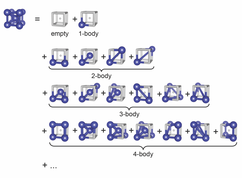
The configuration is decomposed into a sum of clusters as shown in figure 1. Each cluster has a set of associated cluster functions, which are defined as
| (2) |
where and are vectors specifying the order of the single-site basis function and the site variables in the cluster, respectively. and specify the th element of the respective vectors. The use of orthogonal basis functions guarantees that the cluster functions defined in (2) are also orthogonal. The symmetrically equivalent clusters are classified as the same cluster, and the collection of all symmetrically equivalent clusters are denoted with an .
The average value of the cluster functions in cluster is referred to as a correlation function, . The physical quantity, , normalized with the number of atomic sites is then expressed as
| (3) |
where is the multiplicity factor indicating the number of cluster per atom and is the effective cluster interaction (ECI) per occurrence, which needs to be determined. It is noted that the cluster includes the cluster of size zero, which have . Alternatively, (3) can be written in a more explicitly form,
| (4) |
where is the ECI of an empty cluster while in this case corresponds to the clusters of size one and higher. It is often more practical and convenient to express the ECI per atom rather than per occurrence Zhang and Sluiter (2016), in which case and are combined into one term, and (3) becomes
| (5) |
CLEASE uses the ECI per atom (), but interested users can determine the value of based on the values of and .
Theoretically, there is an infinite number of terms in (5) for an infinite crystal, and the resulting expression can represent any scalar function given that appropriate ECI values are found. In practice, sufficient accuracy is often reached with clusters with small number of atoms (e.g., one-, two- and three-body clusters) that are relatively compact in size (e.g., 5 to 7 Å in diameter).
II.2 Cluster Selection & Determination of ECI Values
A crucial element of CE approach is to select relevant clusters from a theoretically infinite number of possible clusters. Many multicomponent systems yield thousands of clusters even when the expansion is limited to relatively compact size and small number of atoms, and they are vastly truncated since only a small fraction of them is needed to achieve the required accuracy. Determining the optimal set of clusters that minimizes the number of clusters without losing its predictive power has been a topic of keen interest in the past decade Zarkevich and Johnson (2004); Blum et al. (2005); Hart et al. (2005); Díaz-Ortiz, Dosch, and Drautz (2007); Lerch et al. (2009), and the cluster selection based on genetic algorithms Blum et al. (2005); Hart et al. (2005); Lerch et al. (2009) was considered to be the most robust method.
More recently, the use of compressive sensing Nelson et al. (2013b) was proposed to efficiently select the clusters and determine their ECIs in one shot. The compressive sensing is based on norm (a special case of norm where ), which is defined as
| (6) |
where is a vector quantity. It is noted that cluster expansion defined in (5) is in the same form as a linear regression model in statistics and machine learning. Therefore, one can treat CE as a linear regression problem and apply regularization techniques based not only on norm but also on any other values, although and norms are most commonly used.
The use of regularization techniques for CE can be illustrated by expressing (5) in a matrix form,
| (7) |
is a matrix containing the correlation functions of the training data where each element in row and column is defined as
| (8) |
is a column vector in which the th element is the physical quantity of the configuration and is a column vector in which th element is .
The simplest way of determining is by using ordinary least squares (OLS) method, which minimizes the residual sum of squared errors (RSS). RSS is defined as
| (9) |
and the minimization of the RSS has a unique solution where
| (10) | ||||
The OLS has two major drawbacks Nelson et al. (2013b). The first is the requirement on which the number of configurations in the training set needs to be larger than the number of clusters being considered. The matrix becomes singular in such a case, and the limitations imposed by the first requirement become more severe for systems consisting of many element types since even strict expansion conditions (i.e., small number of atoms per cluster and compact size) can lead to a large number of clusters. The second drawback is the susceptibility to possible overfitting, which refers to the conditions in which the ECI values are over-tuned to accurately represent of the training set at a cost of losing its predictive power for the new configurations that are not included in the training set. The overfitting also makes the model prone to noise present in the training data because the model attempts to meticulously fit the model to the training data including the noise therein.
Regularization is an efficient technique to address the aforementioned drawbacks of OLS by adding a regularization term to (10). The most common regularization scheme are and regularization, which respectively uses and norm as a regularization term. For regularization, the solution becomes
| (11) |
where is a regularization parameter that controls the weight given to the regularization term. The main benefit of regularization is its promotion of sparsity. In context of CE, the sparsity means a selection of a fewer number of clusters, or many clusters with their ECI values set to zero. It is noted that there is no unique analytical solution for (11), and it needs to be solved iteratively. Unlike regularization, regularization has a unique analytical solution which is expressed as
| (12) | ||||
However, regularization does not promote sparsity, and the resulting solution is likely to contain more clusters than necessary. It is noted that Bayesian compressive sensing Nelson et al. (2013a) scheme is introduced for cluster expansion, which effectively eliminates the parameter in and regularization schemes while promoting sparsity.
Regardless of the fitting technique used, the predictive power of the expansion needs to be assessed to determine its accuracy and reliability. Cross-validation (CV) is a technique used for assessing the prediction accuracy of the model. A leave-one-out (LOO) scheme is most commonly used in CE community, and the LOOCV score is defined as
| (13) |
where is the number of configurations in the training set, is the physical quantity of a structure predicted by CE using structures without a structure and is the calculated physical quantity of structure . While OLS has only one (likely overfitted) solution, and regularization schemes have a solution for each value. The solution — a selection of clusters and their ECI values — that yields the lowest LOOCV score is chosen. Although LOO is the most common cross validation scheme in cluster expansion community, -fold CV is one of the most common schemes used in machine learning community. In a -fold CV scheme, the pool of configurations are randomly partitioned into parts of equal size. The structures in parts are used as training data while the remaining one part is used as a validation set, and the cross validation is repeated times.
II.3 Thermodynamics in Lattice Models
The true benefit of CE is in its ability to predict the expanded scalar quantity based on trained data. An accurate prediction can be made if the CV score of the expanded is sufficiently low, and the prediction speed is very fast on modern computer architecture since it only involves executions of only a small number of simple numerical calculations specified in (5). Such a speed boost allows one to conduct types of analyses that require substantial statistical sampling.
In contrast to zero temperature studies where the system occupies the state with lowest energy, an ensemble of configurations with the lowest free energy are occupied at finite temperature. The free energy is given by Andersen (2012)
| (14) |
where and is the partition function. is the Boltzmann constant and is temperature in Kelvin. It is noted that the DFT energies are obtained for fully relaxed structures without any external forces or pressure. Thus, the resulting thermodynamic quantities are effectively obtained in the NPT ensemble (fixed number of particles, fixed pressure and fixed temperature). However, the energy predicted by CE is only valid for the volume leading to the minimum energy of a particular atomic arrangement, and the volume fluctuations are neglected. The free energy can be calculated by utilizing the exact differential
| (15) | ||||
where is the average internal energy. The free energy can be obtained by a thermodynamic integration from a reference temperature where is known, which can be written as Tuckerman (2010)
| (16) |
Important information of the materials under study such as the stability of ordered/disordered phases can be determined by comparing the free energy of the material at a given composition with respect to the free energies in the pure phases of its constituents.
III Implementation
CLEASE utilizes the existing classes and methods of ASE to perform necessary manipulations and analyses for carrying out CE. Among many adopted features, the most noteworthy are the use of
-
•
an Atoms object to represent an atomic configuration (),
-
•
a built-in database to efficiently store, maintain and share settings, atomic configurations of the training set, values of the correlation functions () and DFT energies,
-
•
Python programming language and modular design to remove the strict input file/format requirements and to enable easy implementation of new features, and
-
•
a Calculator class to determine the physical quantity of a new configuration based on its correlation functions and their ECI values.
It is noted that the evaluation of correlation functions of a new configuration and the determination of physical quantity, , based on ECI values can be a slow process using Python programming language. It is especially true for carrying out Monte Carlo simulations after the CE model training is complete. CLEASE includes an optional external module written in C++ programming language that can be installed to accelerate the critical and repetitive calculations, but the usage of the code remains unchanged even when the external module is installed (i.e., CLEASE automatically determines if the C++ add-on is installed, and uses the C++ version if it is present).
The inheritance of the existing features of ASE allows CLEASE to be fully integrated to ASE where the users can incorporate CE as a part of their research without losing the continuity with the rest of their workflow. The existing users of ASE do not have to install or learn a new CE program nor select a particular DFT package that a CE code supports. In addition to the benefits of integrating CE as a part of ASE, highlights of the features that makes CLEASE versatile and user-friendly include:
-
•
a multicomponent cluster expansion that goes beyond binary systems,
- •
-
•
many methods for selecting clusters and determining ECI values such as OLS, and regularization schemes, Bayesian compressive sensing and genetic algorithm, and
-
•
both leave-one-out and -fold cross validation schemes.
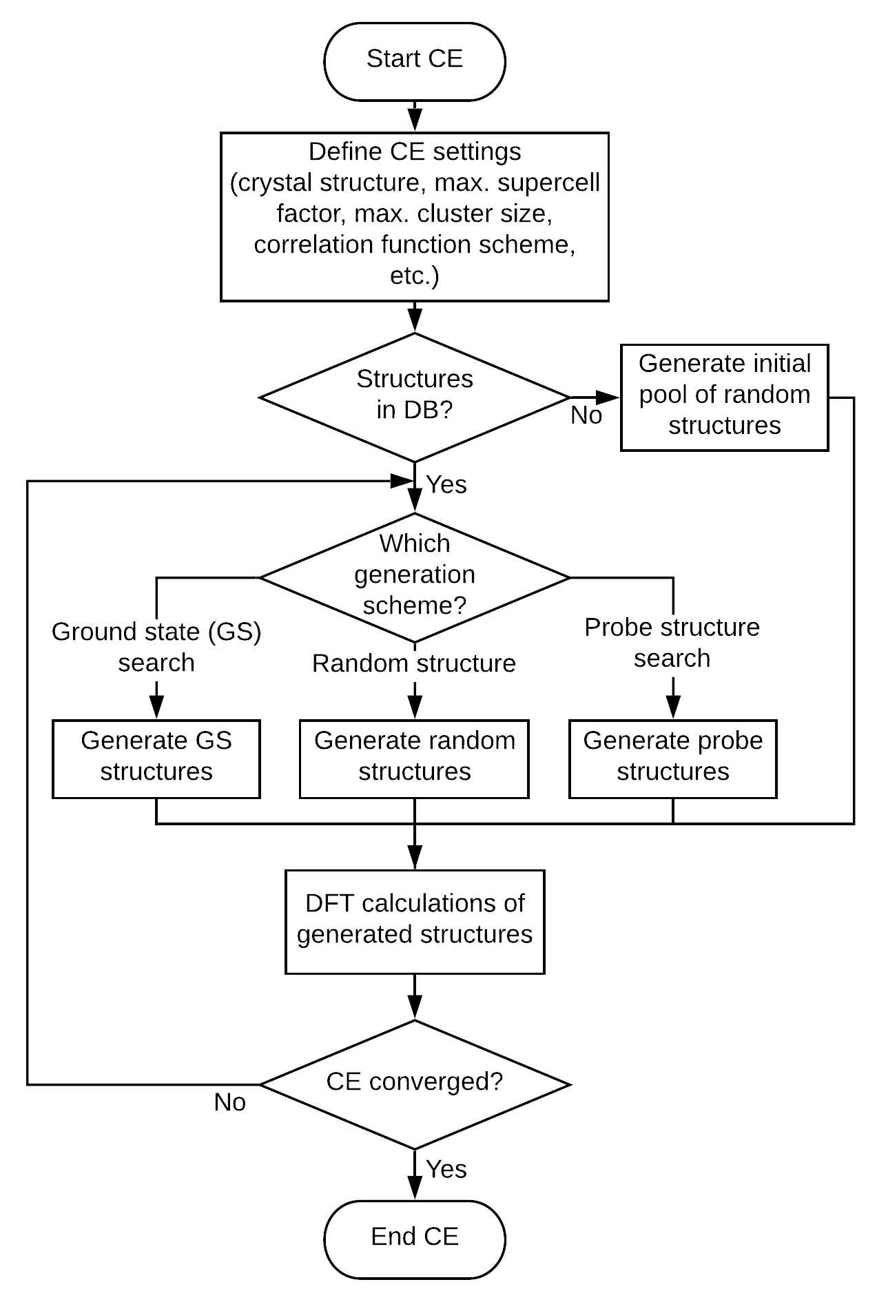
A simple flowchart illustrating the procedure for constructing CE using CLEASE is shown in figure 2. The CLEASE workflow can be divided in to three main components: definition of CE settings, generation of training structures and evaluation of CE convergence. CLEASE takes an object-oriented approach where each component has its own class. The modular design approach not only enables easy implementation of new features but also makes the code flexible to use and intuitive to follow the CE construction and evaluation procedure shown in figure 2. A more detailed description of main components of the procedure is provided below.
III.1 Definition of Cluster Expansion Settings
The most fundamental component is to define which underlying crystal structure to use. ASE offers two functions to generate a crystal structure: bulk and crystal. The bulk function provides a simple way of generating common types of crystal structures by specifying the name of the crystal structure and its lattice constant value(s). The crystal structures supported by the bulk function are simple cubic, face-centered cubic, body-centered cubic, hexagonal close packed, diamond, zinc blende, rocksalt, cesium chloride, fluorite and wurtzite structures. For more complicated crystal structures, a crystal function is used to generate a crystal structure by providing its space group, lattice parameters and scaled coordinates of the unique atomic sites. The definitions of the cluster expansion settings are specified using CEBulk and CECrystal classes, which respectively calls bulk and crystal functions to generate an Atoms object with the user-specified crystal structure.
The maximum size of the supercell (of the primitive cell) on which the DFT calculations are performed is also defined along with the definition of the underlying crystal structure. The maximum supercell size is specified using a supercell_factor parameter, which is an integer corresponding to the product of the absolute values of expansion coefficients (integer weights of a general linear combinations of the unit cell vectors). In other words, if a unit cell has three vectors , and , the configurations in the training set on which the DFT calculations are performed have cell vectors , and , which are defined as
| (17) | ||||
with integer coefficients , and , where . The supercell_factor is then defined as
| (18) |
and all of the cells used in the training set should have coefficients satisfying the condition in (18). Only unique cell shapes are included in the pool by omitting the cells that can be mapped on to the existing cells in the pool by rotation and reflection. The use of supercells with varying sizes and shapes enables the exploration of a larger configurational space without adding extra computational burden compared to using one fixed supercell size and shape. A set of training structures for CE are later generated iteratively from the pool of possible structures that are realizable using these supercells. To reduce the required computational resources, the structures using smaller supercells are generated (and calculated) first, followed by the larger supercells. The users also have a flexibility to select the supercell size using an optional size parameter, which is a matrix (or a nested list in Python) specifying the values of the integer coefficients in (17).
Theoretically, an infinite number of clusters can be generated for a given system. The number of clusters is limited to a finite size in practice, and CLEASE takes an approach to generate all possible clusters that are under the truncation threshold (i.e., a maximum number of atoms in clusters and maximum diameter) specified by the user. A whole or subset of the generated clusters is selected during the convergence evaluation process. By default, up to four-body clusters (i.e., empty, one-, two-, three- and four-body clusters) with their diameters up to 5 Å are generated. The users have an option to define their own threshold settings both at the beginning of the CE procedure and at a later stage of the CE iteration cycles. CLEASE also offers a feature to visualize the generated clusters in order to assist the user to develop an intuition on the generated clusters.
Within the CE formalism, there does not exist a unique set of definitions for basis functions; the basis functions are considered valid if they form a complete set. Consequently, several definitions are used in practice. The two most widely used definitions are the original definitions by Sanchez et al. Sanchez, Ducastelle, and Gratias (1984) and the one later developed by van de Walle van de Walle (2009), which is used in the Alloy Theoretic Automated Toolkit (ATAT) van de Walle (2009); van de Walle, Asta, and Ceder (2002). The two definitions are equally valid, and both are implemented in CLEASE.
CLEASE offers an option to ignore a set of symmetrically inequivalent atomic sites if they are always occupied by one element type for all possible configurations. The contributions of these atoms are not explicitly included in the cluster expansion and are automatically included in the constant term () in (4). For example, lithium metal oxides (\ceLiMO2) with first-row transition metals (M = {Sc, Ti, V, Cr, Mn, Fe, Co, Ni, Cu}) have a rocksalt lattice structure Urban et al. (2016); Urban, Lee, and Ceder (2014) with an exception of \ceLiMnO2, which is orthorhombic Hewston and Chamberland (1987). The rocksalt lattice structure consists of two face-centered cubic sublattices. For the case of the cation-disordered rocksalt lattice \ceLiMO2, one sublattice is occupied by lithium and other metal atoms while the other is occupied by oxygen atoms. The complexity of the CE model of such systems can be reduced to a cation sublattice consisting only of two element types (the oxygen sublattice is ignored). As such, an optional Boolean argument is present in CLEASE to enable/disable the reduction of the complexity of the model by ignoring the such atoms if they exist in the system.
A range of compositions (or concentration) of the system to be studied is specified using a Concentration class. First, the constituting elements of the system are categorized into the basis which they belong. For example, \ceLiVO2 in a rocksalt lattice structure is expressed using two lists: [‘\ceLi’, ‘\ceV’] and [‘\ceO’]. It is noted that CE needs to keep track of the location of vacancies when they are present in the system. The location of vacancies are tracked by treating a vacancy as a regular atom with its atomic symbol set to ‘X’ or atomic number set to zero. The \ceLiVO2 with \ceLi vacancies is then expressed using [‘\ceLi’, ‘\ceV’, ‘X’] and [‘\ceO’].
The range of each element (including vacancies) can be specified in one of the two convenient methods built in to the Concentration class. The simplest method is to specify the concentration range of each constituting element by calling set_conc_ranges method in Concentration class. For the cases where concentrations of two or more elements depend on one another, one can specify concentration range using set_conc_formula_unit method where the relationships between the concentrations of two or more elements can be expressed in a list of strings. For the example of \ceLiVO2 with \ceLi vacancies, a list of strings that specifies relationship between the number of \ceLi atoms and the number of vacancies, [“LixV1X1-x”, “O2”], is passed as an argument to the set_conc_formula_unit method. Another argument specifying the range of the concentration variable, e.g., {‘x’: (0, 1)}, is also passed to the set_conc_formula_unit method in order to specify the concentration range of Li and Li vacancies. The concentration ranges specified by either set_conc_ranges or set_conc_formula_unit methods are internally interpreted in the Concentration class as a list of linear equations that specify (1) the relationships of the concentrations of constituting elements and (2) their upper/lower bounds. The advanced users can alternatively specify the coefficients of the linear equations used in the Concentration class if a greater flexibility is needed in specifying the concentration ranges.
III.2 Generation of Training Structures
CLEASE uses NewStructures class to generate training structures, which provides three different methods perform the task. The first and most trivial method is to generate a set of random structures. This method serves to generate an initial pool consisting of a small number of structures. The random generation method is used in the first iteration cycle of CE construction as shown in figure 2. An initial cluster expansion is capable of making a first set of predictions albeit with a low accuracy. It is noted that all of the generated training structures, along with their correlation function values, are stored in a database file.
Once the initial CE is constructed, the user is given three different choices for introducing an additional set of training structures. The first and most straightforward option is to keep generating random structures. Although trivial, generating random structures is claimed to be the best strategy when compressive sensing is used to select clusters Nelson et al. (2013b). The second method is to generate ground-state and other low-energy structures based on current cluster expansion (i.e., based on the pool of structures already calculated) van de Walle and Ceder (2002), which have the enthalpies of formation either on or near the convex hull Urban, Seo, and Ceder (2016). The inclusion of ground-state and near-ground-state structures serves an important purpose of increasing the accuracy in predicting the correct ground states. A global minimization technique can be used to generate (near) ground-state configurations, and CLEASE uses a simulated annealing technique.
The last method of generating the training set is referred to as a “probe structure” method Seko, Koyama, and Tanaka (2009); Seko and Tanaka (2014). The probe structure method introduces a new structure that minimizes the mean variance of the predicted physical quantity . The mean variance of the predicted quantity is written as Seko, Koyama, and Tanaka (2009)
| (19) | ||||
where is the variance of the error in the training set, is the covariance matrix of the correlation functions of the training set and is a vector of the mean correlation functions of the structures in the training set. The probe structure is the one that reduce the value of the most when introduced to the training set, which is found using the simulated annealing procedure.
The newly generated structures are compared with the existing structures in the training set in order to avoid introducing duplicate structures. We adopted the structure comparison algorithm developed by Lonie and Zurek Lonie and Zurek (2012) to identify equivalent structures. It is desirable to have the new structure compared against the existing structures in the training set as efficiently as possible. As a first step, the structures that have different chemical composition than the newly generated structure are filtered, and the new structure is compared only with the remaining structures. Once the candidate transformations for mapping the new structure onto one structure in the database are identified using the algorithm suggested by Lonie and Zurek, we note that exactly the same transformations can be used for the remaining structures in the database. Therefore, the structure comparison algorithm implemented in ASE is optimized for the case where one structure is to be compared against many.
In addition to the aforementioned methods of generating the training structures, CLEASE also offers a built-in function to import structures to the database. The import function also has an option to specify the calculated value, which allows users to easily import the previously calculated results.
III.3 Evaluation of Cluster Expansion Convergence
An evaluation process to determine the convergence of CE includes a selection of clusters, a determination of their ECI values and an assessment of the LOO or -fold CV score using the selected clusters and their ECI values. An entire evaluation process is performed using an Evaluate class.
The simplest way to determine the ECI values of the generated clusters is by using OLS to minimize residual sum of squared errors (RSS). It is highly likely that the ECI values found using OLS are overfitted. Therefore, Bayesian compressive sensing and and regularization methods are implemented, and it is highly recommended to use a regularization methods to select clusters and evaluate their ECI values.
A default option in the Evaluate class is to include all of the clusters generated using the cluster truncation conditions specified in CEBulk or CECrystal class, and either the entire or a subset of these clusters are selected for fitting depending on the method used. The Evaluate class provides additional options in which the users can select a subset of the generated clusters to perform any of OLS, Baysian compressive sensing and and regularization. The first option is by manually specifying which clusters to include, while the second option is to provide a stricter truncation conditions than the ones set in the CEBulk or CECrystal class. The first option allows the Evaluate class to be used in conjunction with other cluster selection methods such as genetic algorithm. For example, a user can optionally use genetic algorithm (included in CLEASE as a separate GAFit class) to pre-screen a large cluster pool and subsequently pass a subset of clusters to the Evaluate class. The feature to freely select a subset of a large pool of clusters along with the use of OLS, Bayesian compressive sensing and and regularization methods allows the users to easily experiment with various settings to understand how the system behaves and to optimize the ECI values for achieving the lowest LOOCV score.
To further assist the evaluation process, the Evaluate class contains two built-in methods that automatically determine the LOOCV when a regularization method is used. The first method, plot_fit, determines and stores the selected clusters and their ECI values for a value of regularization parameter () specified by the user. It also plots the fit of all data points in the training set to their calculated values and presents the LOO/-fold CV score of the specified value. Since the most cumbersome task in determining the convergence of CE is finding the optimal value that yields the lowest CV score, another method, plot_CV, is also implemented. It takes a range and number of values to evaluate as inputs and returns the best value in the specified range along with its LOO/-fold CV score. The plot_CV method also plots LOO/-fold CV score as a function of and provides an option to store the results in a log file such that the users can add more values to the list at a later stage without having to re-evaluate the same values in the process.
III.4 Metropolis Monte Carlo and Simulated Annealing
The user can perform statistical sampling of the system on a larger simulation cell once the cluster expansion is constructed. The final selection of cluster and their ECI values can be stored and passed to other classes to conduct statistical analyses. A separate Calculator class for cluster expansion is implemented in ASE. The Clease calculator class takes a list of clusters and their ECI values as inputs, and the users can select what type of trial moves are allowed. The sampling in the canonical ensemble allows the swapping two atoms with different constraint conditions (i.e., swap any two atoms, swap any two atoms in the same basis, swap two nearest neighbors, swap two nearest neighbors in the same basis) while the semi-grand canonical ensemble allows changing the type of occupying element at a random site.
The evaluation of the physical quantity is performed using (5), which is a fast because the Clease calculator keeps track of the changes in the Atoms object to update the correlation functions. When the physical quantity being modeled is energy, a trial move of the standard Metropolis algorithm has an acceptance probability Thijssen (2007)
| (20) |
where and are the energy of the new and old configuration, respectively. As the Clease calculator keeps track of the change in the Atoms object after each move, updating the correlation functions is restricted to the contributions of one and two atoms for the semi-grand canonical ensemble and canonical ensemble, respectively.
IV Examples
Here, we present two example systems to illustrate the capabilities of the CLEASE code. The first example illustrates the investigation of a Au–Cu binary alloy. The second example shows the cluster expansion on a more complex \ceLi2CrO2F system consisting of four types of elements and vacancy. All of the interactions of cluster expansions are computed from DFT calculations of energies, and the computational settings used for generating the results shown in this section are specified in section V.
IV.1 Au–Cu Alloy
The binary Au–Cu alloy system is studied at temperatures ranging from 100 K to 800 K over the entire composition range. The resulting values obtained for both and regularization are shown in figure 3. The ECI value of the empty cluster is found to be eV/atom for both cases, and the ECI value of the one-body cluster is 0.27 eV/atom and 0.13 eV/atom for and regularization, respectively. The ECI values of empty and one-body clusters are not included in figure 3 for better visibility. The LOOCV score for the - and -regularized fit were 4.49 meV/atom and 4.67 meV/atom, respectively. The regularization scheme yields a slightly lower CV score despite having a smaller number of clusters (-regularized fit has 20 clusters while the -regularized fit has 34 clusters).
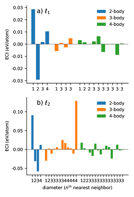
A qualitative information on the thermodynamic behavior of the system can be extracted by inspecting the ECI values for simple binary system. Based on the fact that the energetically favorable configurations have DFT energies that are more negative than less favorable ones and that the two site variables are or , one can infer that a positive ECI value of the pair interaction term means that a pair consisting of two different elements is energetically preferred at a low temperature. It can be seen in figure 3 that the ECIs of the nearest-neighbor and second nearest-neighbor pairs are positive and positive, respectively. The signs indicate that the Au–Cu system energetically favors the strong mixing of the constituting elements such that the alternating patterns found in L10- and L12-type ordered structures are likely to emerge, which is in a good agreement with experimental and computational observations van de Walle and Ceder (2002); Wei et al. (1987); Ozoliņš, Wolverton, and Zunger (1998a, b); Wolverton, Ozoliņš, and Zunger (1998); Lysgaard et al. (2015); Massalski et al. (1986); Hultgren, Hawkins, and Desai (1973); Fedorov and Volkov (2016).
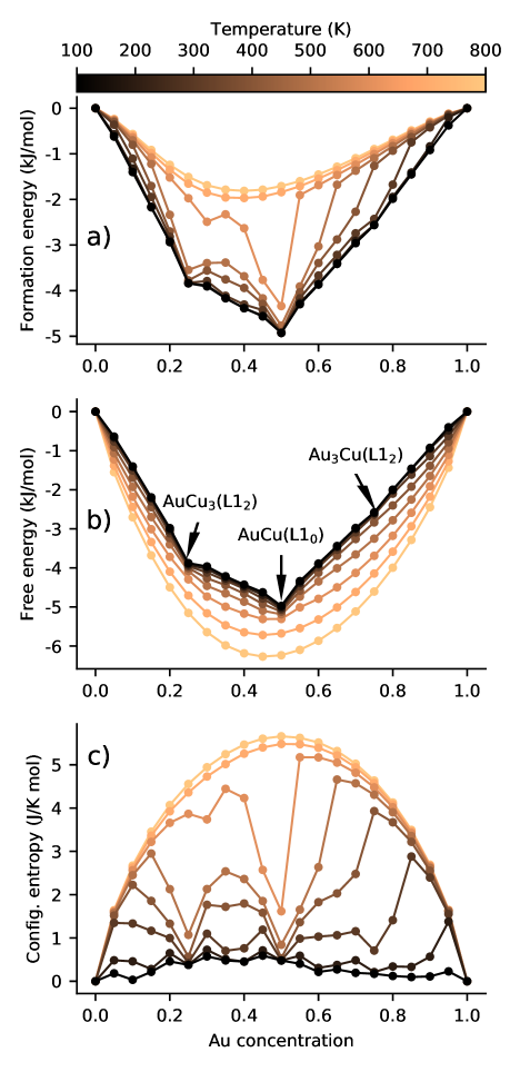
It is experimentally determined that Au–Cu alloys have three ordered phases at low temperatures Massalski et al. (1986); Hultgren, Hawkins, and Desai (1973); Fedorov and Volkov (2016): \ceAuCu3, \ceAuCu and \ceAu3Cu. Furthermore, the transition temperatures for \ceAuCu3, \ceAuCu and \ceAu3Cu are reported to be 663 K, 683 K and 490 K, respectively, and they are often used as reference values for assessing the computational models van de Walle and Ceder (2002); Wei et al. (1987); Ozoliņš, Wolverton, and Zunger (1998a). The formation energy, free energy of formation and configurational entropy are obtained through Metropolis Monte Carlo simulations and are shown in figure 4. As the CE is trained with fully relaxed structures (zero pressure), the formation energy is determined using
| (21) |
where is the internal energy of the configuration, is the gold concentration, is the internal energy of pure gold and is the internal energy of pure copper. Similarly, the free energy of formation is obtained by subtracting the weighted average of the free energy for the pure phases. The configurational entropy is given by the difference between the internal energy and the free energy, divided by the temperature at which the Monte Carlo is sampled. The three ordered phases (\ceAuCu3, \ceAuCu and \ceAu3Cu) are found on the convex hull of the free energy of formation in figure 4b. Furthermore, the entropy of the ordered phases form local minima as shown in figure 4c. As the temperature increases, the free energy becomes a smooth convex curve with a minimum at around composition, and the system is in a random phase with no short-range order.
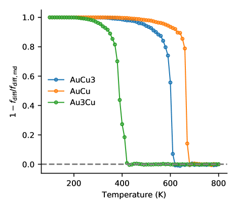
An accurate estimate of the order/disorder transition temperature can be found by tracking the evolution of an order parameter. The average fraction of sites having a different element than the same site in the ground state, , is tracked as the system evolves. is normalized by the expected fraction of different sites in a random phase, , and an order parameter, , is defined as
| (22) |
The order parameter is is used for detecting the phase transition as shown in figure 5. The computationally predicted order/disorder transition temperature of \ceAuCu3, \ceAuCu and \ceAu3Cu are around 600 K, 665 K and 385 K, respectively, which are in a good agreement with the experimental reference values Massalski et al. (1986); Hultgren, Hawkins, and Desai (1973); Fedorov and Volkov (2016).
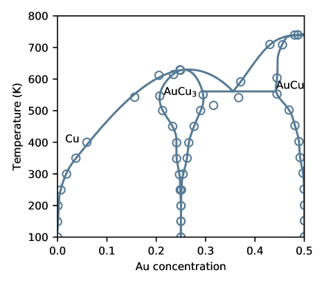
One of the most common way to describe the characteristics of a binary alloy is by constructing a phase diagram. A phase diagram can be generated computationally using a semi-grand canonical MC where a grand potential is obtained via thermodynamic integration in (16) at fixed chemical potentials. The integration starts from the low temperature limit for the ordered phases and from the high temperature limit for disordered phases where the free energy per atom is given by . The phase boundary between two phases is identified by locating the intersection point between the grand potential in the two co-existing phases. The phase diagram generated via semi-grand canonical MC is shown in figure 6. The phase diagram closely resembles the phase diagrams constructed from the experimental measurements Massalski et al. (1986); Hultgren, Hawkins, and Desai (1973); Fedorov and Volkov (2016) and is also in a qualitatively agreement with the phase diagrams constructed from computational results van de Walle and Ceder (2002); Wei et al. (1987); Walle and Asta (2002).
IV.2 Lithium Chromium Oxyfluoride
One of the recent focus areas of lithium-ion battery research is the development of high-capacity cathode materials. Lithium metal oxyfluorides (\ceLi2MO2F, {V, Cr, Mn, Ti, Ni, }) is a family of materials that is at the forefront of the current research. The challenges for studying \ceLi2MO2F is in the vast size of the configurational space, which exhibit not only the cation disorder commonly found in lithium metal oxides Abdellahi et al. (2016a); Urban et al. (2016) but also anion disorder which is also present due to the mixed O/F composition Chen et al. (2015, 2016). The fact that the underlying crystal structure of \ceLi2MO2F can vary at different lithiation levels Cambaz et al. (2016) adds the complexity to investigate their properties. It is, however, known that the most predominant crystal structure is of disordered rocksalt type Ren et al. (2015), particularly at high-lithiation levels. We therefore show an example CE study of \ceLi2CrO2F in a rocksalt lattice configuration.
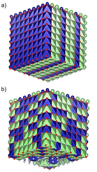
The Monte Carlo annealing study reveals that \ceLi2CrO2F (i.e., fully lithiated compound) takes a layered structure at room temperature (293 K) as shown in figure 7a. The layer structure shows a –Li–F–Li–O–Cr–O– pattern, which is similar to a –Li–O–M–O– layered pattern observed in lithium metal oxides Urban et al. (2016); Mizushima et al. (1981); Van der Ven and Ceder (2004). The layered structure is lost upon delithiation, which leads to disordered structures as shown in figure 7b. The emergence of disordered structures agrees well with the previous experimental observations Chen et al. (2016); Ren et al. (2015), and it is important to model the disordered atomic arrangement as it has a direct link to the Li transport mechanism (e.g., a presence of zero-transition-metal pathways Urban et al. (2016); Urban, Lee, and Ceder (2014); Lee et al. (2014)).
Thermodynamics quantities of LixCrO2F can be extracted with the same procedure described for the Au–Cu system. One of the most crucial thermodynamic parameters for characterizing cathode materials for Li-ion batteries is the free energy as it is directly linked to the operating voltage of the cell. The operating voltage of LixCrO2F is defined as
| (23) | ||||
where is the chemical potential in eV per Li atom, is an electron charge and is the free energy of LixCrO2F in eV per formula unit. Li metal is used as an anode and thus, is constant.
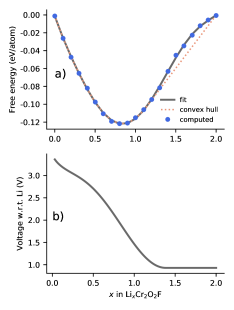
The free energy of LixCrO2F and its voltage profile at 293 K are shown in figure 8. The free energy in figure 8a has three parts: free energy values computed from MC simulations, a smooth curve fitted to the computed values (using Redlich-Kister polynomials Redlich and Kister (1948)) and a convex hull of the fitted curve. The curve fit is used for generating the voltage plot because the derivative of the free energy used for calculating the voltage values are susceptible to small noise that are present in the MC simulation results. Furthermore, a range in which the free energy curve is above the convex hull represents the region where a phase transition occurs: the cathode forms a mixture of two phases at which the fitted curve and the convex hull intersect. The voltage profile in figure 8b is generating using (23) where the values on the convex hull are used for . The voltage profile in figure 8b is in a good agreement with those observed experimentally Chen et al. (2016); Ren et al. (2015).
V Methods
V.1 Density Functional Theory Calculations
All of the calculations are performed with the Vienna Ab initio Simulation Package (VASP) Kresse and Hafner (1993, 1994); Kresse and Furthmüller (1996, 1996) using the projector augmented-wave (PAW) method Blöchl (1994). The generalized gradient approximation as parametrized by Perdew, Burke and Ernzerhof Perdew, Burke, and Ernzerhof (1996) is used as the exchange-correlation functional. It is important to have a consistent and accurate dataset (i.e., DFT calculations with high energy cutoff and -point mesh density) in order to minimize the numerical noise introduced to the CE training. The plane-wave cutoff of 500 eV is used, and both the cell and atomic positions are fully relaxed such that all the forces are smaller than 0.02 eV/Å. A rotationally invariant Hubbard U correction Anisimov, Zaanen, and Andersen (1991); Cococcioni and de Gironcoli (2005) is applied to the orbital of Cr with the value of 3.7 eV. The calculations are performed with supercells containing up to 18 and 54 atoms for Au–Cu alloy and \ceLi2CrO2F systems, respectively. Integrations over the Brillouin zone were carried out using the Monkhorst-Pack scheme Monkhorst and Pack (1976) with a grid with a maximal interval of 0.04 Å-1.
V.2 Cluster Expansion Model
The CE model for Au–Cu alloy and LixCrO2F are trained using 34 and 390 DFT calculations, respectively. CE model is trained for the entire composition range of Au–Cu alloy (from pure Au to pure Cu) and LixCrO2F on a rocksalt lattice with ranges from 0 to 2. Up to four-body clusters with the maximum diameter of 6.0 Å are generated for Au–Cu alloy. Up to four-body clusters are generated for LixCrO2F with the maximum diameter of 7.0 for two- and three-body clusters and 4.5 Å for four-body clusters. and regularization schemes with the regularization parameter ranging from to are assessed at various maximum radii to find the optimal setting that leads to the lowest LOOCV score. For the Au–Cu alloy, regularization with the maximum diameter of 6.0 Å, 5.0 Å and 5.0 Å for 2-, 3- and 4-body clusters, respectively, yields the lowest LOOCV score of 4.49 meV/atom. The minimum LOOCV score achieved using regularization scheme is 4.67 meV/atom when the maximum diameter is set to 6.0 Å, 6.0 Å and 5.0 Å for 2-, 3- and 4-body clusters, respectively. Similarly, regularization performed better than regularization on LixCrO2F with the lowest LOOCV score of 21.38 meV/atom (maximum diameter set to 7.0 Å, 7.0 Å and 4.5 Å for 2-, 3- and 4-body clusters, respectively). It is noted that although the LOOCV of LixCrO2F seems larger compared to that of Au–Cu, it should be taken into account that the cohesive energy of metallic alloys are in general much smaller than those of oxyfluorides.
V.3 Metropolis Monte Carlo Simulations
For Au–Cu alloy, Metropolis Monte Carlo simulations are carried out using a supercell consisting of 1,000 atoms for determining thermodynamic quantities. The system is equilibrated with 100 sweeps, and an average energy is collected through an additional 2,000 sweeps at each temperature for determining the thermodynamic quantities. A supercell consisting of 27,000 atoms is used to determine the transition temperatures and to construct a phase diagram. The transition temperatures are determined by equilibrating the systems with 100 sweeps, followed by sampling the order parameter via an additional 1,000 sweeps. A phase diagram is generated by performing a semi-grand canonical MC, where the system is equilibrated using 100 sweeps, followed an additional 1,000 sweeps to obtain an average semi-grand canonical energy at each temperature at a fixed chemical potential. A cell consisting of 1,458 atoms is used for LixCrO2F. The temperature is gradually lowered from 10,000 K, and the structures are equilibrated at each temperature via 100 sweeps to ensure that the system is equilibrated before sampling. The average energy is then sampled via 1,000 sweeps at each temperature.
VI Conclusions
We present the implementation of CLEASE, which fully integrates the cluster expansion method to ASE package. The aim of the developed code is to make cluster expansion more accessible to non-specialists and to incorporate modern machine learning techniques to cluster expansion method in one comprehensive and versatile package. The use of the popular Python programming language and implementing the code as a part of widely used ASE package lowers the barrier for the newcomers to the field to easily learn and use CE as a part of their research methods. By automatically generating clusters and calculating the correlation functions of both semi-automatically generated and user-supplied structures, it minimizes both the possible introduction of user errors and complicated process of constructing/evaluating the cluster expansion. The capability of CLEASE is presented with two example usage cases with a different level of system complexity. The examples demonstrate that CE can correctly predict the material behavior that require statistical sampling on a large simulation cell.
VII Acknowledgements
This project has received funding from the European Union’s Horizon 2020 research and innovation programme under grant agreement No 711792 (FET‐OPEN project LiRichFCC). Authors thank valuable discussions with Dr. Juhani Teeriniemi and Prof. Kari Laasonen. JMGL acknowledges support from the Villum Foundation’s Young Investigator Programme (4th round, project: In silico design of efficient materials for next generation batteries. Grant number: 10096).
References
- Sanchez, Ducastelle, and Gratias (1984) J. M. Sanchez, F. Ducastelle, and D. Gratias, “Generalized cluster description of multicomponent systems,” Physica A: Statistical Mechanics and its Applications 128, 334–350 (1984).
- Fontaine (1994) D. D. Fontaine, “Cluster Approach to Order-Disorder Transformations in Alloys,” in Solid State Physics, Vol. 47, edited by H. Ehrenreich and D. Turnbull (Academic Press, 1994) pp. 33–176.
- Zunger (1994) A. Zunger, “First-Principles Statistical Mechanics of Semiconductor Alloys and Intermetallic Compounds,” in Statics and Dynamics of Alloy Phase Transformations, edited by P. E. A. Turchi and A. Gonis (Springer US, Boston, MA, 1994) pp. 361–419.
- Asta, Ozolins, and Woodward (2001) M. Asta, V. Ozolins, and C. Woodward, “A first-principles approach to modeling alloy phase equilibria,” JOM 53, 16–19 (2001).
- van de Walle (2008) A. van de Walle, “A complete representation of structure-property relationships in crystals,” Nature Materials 7, 455–458 (2008).
- Zhang and Sluiter (2016) X. Zhang and M. H. F. Sluiter, “Cluster Expansions for Thermodynamics and Kinetics of Multicomponent Alloys,” Journal of Phase Equilibria and Diffusion 37, 44–52 (2016).
- Magri and Zunger (1991) R. Magri and A. Zunger, “Real-space description of semiconducting band gaps in substitutional systems,” Physical Review B 44, 8672–8684 (1991).
- Franceschetti and Zunger (1999) A. Franceschetti and A. Zunger, “The inverse band-structure problem of finding an atomic configuration with given electronic properties,” Nature 402, 60–63 (1999).
- Geng, Sluiter, and Chen (2005) H. Y. Geng, M. H. F. Sluiter, and N. X. Chen, “Cluster expansion of electronic excitations: Application to fcc Ni–Al alloys,” The Journal of Chemical Physics 122, 214706 (2005).
- Wang et al. (2015) R. Wang, X. Li, L. Liu, J. Lee, D.-H. Seo, S.-H. Bo, A. Urban, and G. Ceder, “A disordered rock-salt Li-excess cathode material with high capacity and substantial oxygen redox activity: Li1.25Nb0.25Mn0.5O2,” Electrochemistry Communications 60, 70–73 (2015).
- Abdellahi et al. (2016a) A. Abdellahi, A. Urban, S. Dacek, and G. Ceder, “The Effect of Cation Disorder on the Average Li Intercalation Voltage of Transition-Metal Oxides,” Chemistry of Materials 28, 3659–3665 (2016a).
- Abdellahi et al. (2016b) A. Abdellahi, A. Urban, S. Dacek, and G. Ceder, “Understanding the Effect of Cation Disorder on the Voltage Profile of Lithium Transition-Metal Oxides,” Chemistry of Materials 28, 5373–5383 (2016b).
- Urban et al. (2016) A. Urban, I. Matts, A. Abdellahi, and G. Ceder, “Computational Design and Preparation of Cation-Disordered Oxides for High-Energy-Density Li-Ion Batteries,” Advanced Energy Materials 6, 1600488 (2016).
- Kitchaev et al. (2018) D. A. Kitchaev, Z. Lun, W. D. Richards, H. Ji, R. J. Clément, M. Balasubramanian, D.-H. Kwon, K. Dai, J. K. Papp, T. Lei, B. D. McCloskey, W. Yang, J. Lee, and G. Ceder, “Design principles for high transition metal capacity in disordered rocksalt Li-ion cathodes,” Energy & Environmental Science 11, 2159–2171 (2018).
- Hjorth Larsen et al. (2017) A. Hjorth Larsen, J. Jørgen Mortensen, J. Blomqvist, I. E. Castelli, R. Christensen, M. Dułak, J. Friis, M. N. Groves, B. Hammer, C. Hargus, E. D. Hermes, P. C. Jennings, P. Bjerre Jensen, J. Kermode, J. R. Kitchin, E. Leonhard Kolsbjerg, J. Kubal, K. Kaasbjerg, S. Lysgaard, J. Bergmann Maronsson, T. Maxson, T. Olsen, L. Pastewka, A. Peterson, C. Rostgaard, J. Schiøtz, O. Schütt, M. Strange, K. S. Thygesen, T. Vegge, L. Vilhelmsen, M. Walter, Z. Zeng, and K. W. Jacobsen, “The atomic simulation environment–a Python library for working with atoms,” Journal of Physics: Condensed Matter 29, 273002 (2017).
- Zarkevich and Johnson (2004) N. A. Zarkevich and D. D. Johnson, “Reliable First-Principles Alloy Thermodynamics via Truncated Cluster Expansions,” Physical Review Letters 92, 255702 (2004).
- Meng and Arroyo-de Dompablo (2009) Y. S. Meng and M. E. Arroyo-de Dompablo, “First principles computational materials design for energy storage materials in lithium ion batteries,” Energy & Environmental Science 2, 589 (2009).
- van de Walle (2009) A. van de Walle, “Multicomponent multisublattice alloys, nonconfigurational entropy and other additions to the Alloy Theoretic Automated Toolkit,” Calphad 33, 266–278 (2009), 0906.1608 .
- Nelson et al. (2013a) L. J. Nelson, V. Ozoliņš, C. S. Reese, F. Zhou, and G. L. W. Hart, “Cluster expansion made easy with Bayesian compressive sensing,” Physical Review B 88, 155105 (2013a).
- Nelson et al. (2013b) L. J. Nelson, G. L. W. Hart, F. Zhou, and V. Ozoliņš, “Compressive sensing as a paradigm for building physics models,” Physical Review B 87, 035125 (2013b).
- Seko and Tanaka (2014) A. Seko and I. Tanaka, “Cluster expansion of multicomponent ionic systems with controlled accuracy: importance of long-range interactions in heterovalent ionic systems,” Journal of Physics: Condensed Matter 26, 115403 (2014).
- Mueller and Ceder (2010) T. Mueller and G. Ceder, “Exact expressions for structure selection in cluster expansions,” Physical Review B 82, 184107 (2010).
- Blum et al. (2005) V. Blum, G. L. W. Hart, M. J. Walorski, and A. Zunger, “Using genetic algorithms to map first-principles results to model Hamiltonians: Application to the generalized Ising model for alloys,” Physical Review B 72, 165113 (2005).
- Hart et al. (2005) G. L. W. Hart, V. Blum, M. J. Walorski, and A. Zunger, “Evolutionary approach for determining first-principles hamiltonians,” Nature Materials 4, 391–394 (2005).
- Díaz-Ortiz, Dosch, and Drautz (2007) A. Díaz-Ortiz, H. Dosch, and R. Drautz, “Cluster expansions in multicomponent systems: Precise expansions from noisy databases,” Journal of Physics Condensed Matter 19 (2007), 10.1088/0953-8984/19/40/406206.
- Lerch et al. (2009) D. Lerch, O. Wieckhorst, G. L. W. Hart, R. W. Forcade, and S. Müller, “UNCLE: a code for constructing cluster expansions for arbitrary lattices with minimal user-input,” Modelling and Simulation in Materials Science and Engineering 17, 055003 (2009).
- Andersen (2012) J. O. Andersen, Introduction to statistical mechanics (Akademica Publishing, 2012).
- Tuckerman (2010) M. E. Tuckerman, Statistical mechanics: theory and molecular simulation (Oxford University Press, 2010).
- van de Walle, Asta, and Ceder (2002) A. van de Walle, M. Asta, and G. Ceder, “The alloy theoretic automated toolkit: A user guide,” Calphad 26, 539–553 (2002).
- Urban, Lee, and Ceder (2014) A. Urban, J. Lee, and G. Ceder, “The Configurational Space of Rocksalt-Type Oxides for High-Capacity Lithium Battery Electrodes,” Advanced Energy Materials 4, 1400478 (2014).
- Hewston and Chamberland (1987) T. Hewston and B. Chamberland, “A Survey of first-row ternary oxides LiMO2 (M = Sc-Cu),” Journal of Physics and Chemistry of Solids 48, 97–108 (1987).
- van de Walle and Ceder (2002) A. van de Walle and G. Ceder, “Automating first-principles phase diagram calculations,” Journal of Phase Equilibria 23, 348 (2002).
- Urban, Seo, and Ceder (2016) A. Urban, D. H. Seo, and G. Ceder, “Computational understanding of Li-ion batteries,” npj Computational Materials 2 (2016), 10.1038/npjcompumats.2016.2.
- Seko, Koyama, and Tanaka (2009) A. Seko, Y. Koyama, and I. Tanaka, “Cluster expansion method for multicomponent systems based on optimal selection of structures for density-functional theory calculations,” Physical Review B 80, 165122 (2009).
- Lonie and Zurek (2012) D. C. Lonie and E. Zurek, “Identifying duplicate crystal structures: XtalComp, an open-source solution,” Computer Physics Communications 183, 690–697 (2012).
- Thijssen (2007) J. Thijssen, Computational Physics (Cambridge University Press, 2007).
- Wei et al. (1987) S. H. Wei, A. A. Mbaye, L. G. Ferreira, and A. Zunger, “First-principles calculations of the phase diagrams of noble metals: Cu-Au, Cu-Ag, and Ag-Au,” Physical Review B 36, 4163–4185 (1987).
- Ozoliņš, Wolverton, and Zunger (1998a) V. Ozoliņš, C. Wolverton, and A. Zunger, “Cu-Au, Ag-Au, Cu-Ag, and Ni-Au intermetallics: First-principles study of temperature-composition phase diagrams and structures,” Physical Review B 57, 6427–6443 (1998a).
- Ozoliņš, Wolverton, and Zunger (1998b) V. Ozoliņš, C. Wolverton, and A. Zunger, “First-principles theory of vibrational effects on the phase stability of Cu-Au compounds and alloys,” Physical Review B 58, R5897–R5900 (1998b).
- Wolverton, Ozoliņš, and Zunger (1998) C. Wolverton, V. Ozoliņš, and A. Zunger, “First-principles theory of short-range order in size-mismatched metal alloys: Cu-Au, Cu-Ag, and Ni-Au,” Physical Review B 57, 4332–4348 (1998).
- Lysgaard et al. (2015) S. Lysgaard, J. S. G. Mýrdal, H. A. Hansen, and T. Vegge, “A DFT-based genetic algorithm search for AuCu nanoalloy electrocatalysts for CO2 reduction,” Physical Chemistry Chemical Physics 17, 28270–28276 (2015).
- Massalski et al. (1986) T. B. Massalski, J. Murray, L. Bennett, and H. Baker, “Binary alloy phase diagrams. vol. i and ii,” American Society for Metals, 1986, , 2224 (1986).
- Hultgren, Hawkins, and Desai (1973) R. Hultgren, D. T. Hawkins, and P. D. Desai, “Selected values of the thermodynamic properties of binary alloys,” (American Society for Testing and Materials, 1973).
- Fedorov and Volkov (2016) P. P. Fedorov and S. N. Volkov, “Au–Cu Phase Diagram,” Russian Journal of Inorganic Chemistry 61, 772–775 (2016).
- Walle and Asta (2002) A. V. D. Walle and M. Asta, “Self-driven lattice-model Monte Carlo simulations of alloy thermodynamic properties and phase diagrams,” Modelling and Simulation in Materials Science and Engineering 10, 521–538 (2002).
- Chen et al. (2015) R. Chen, S. Ren, M. Knapp, D. Wang, R. Witter, M. Fichtner, and H. Hahn, “Disordered lithium-rich oxyfluoride as a stable host for enhanced Li+ intercalation storage,” Advanced Energy Materials 5, 1–7 (2015).
- Chen et al. (2016) R. Chen, S. Ren, X. Mu, E. Maawad, S. Zander, R. Hempelmann, and H. Hahn, “High-Performance Low-Temperature Li + Intercalation in Disordered Rock-Salt Li-Cr-V Oxyfluorides,” ChemElectroChem 3, 892–895 (2016).
- Cambaz et al. (2016) M. A. Cambaz, B. P. Vinayan, O. Clemens, A. R. Munnangi, V. S. K. Chakravadhanula, C. Kübel, and M. Fichtner, “Vanadium Oxyfluoride/Few-Layer Graphene Composite as a High-Performance Cathode Material for Lithium Batteries,” Inorganic Chemistry 55, 3789–3796 (2016).
- Ren et al. (2015) S. Ren, R. Chen, E. Maawad, O. Dolotko, A. A. Guda, V. Shapovalov, D. Wang, H. Hahn, and M. Fichtner, “Improved Voltage and Cycling for Li+ Intercalation in High-Capacity Disordered Oxyfluoride Cathodes,” Advanced Science 2, 1500128 (2015).
- Mizushima et al. (1981) K. Mizushima, P. Jones, P. Wiseman, and J. Goodenough, “LixCoO2 (): A new cathode material for batteries of high energy density,” Solid State Ionics 3-4, 171–174 (1981).
- Van der Ven and Ceder (2004) A. Van der Ven and G. Ceder, “Ordering in Lix(Ni0.5Mn0.5)O2 and its relation to charge capacity and electrochemical behavior in rechargeable lithium batteries,” Electrochemistry Communications 6, 1045–1050 (2004).
- Lee et al. (2014) J. Lee, A. Urban, X. Li, D. Su, G. Hautier, and G. Ceder, “Unlocking the Potential of Cation-Disordered Oxides for Rechargeable Lithium Batteries,” Science 343, 519–522 (2014).
- Redlich and Kister (1948) O. Redlich and A. T. Kister, “Algebraic representation of thermodynamic properties and the classification of solutions,” Industrial & Engineering Chemistry 40, 345–348 (1948).
- Kresse and Hafner (1993) G. Kresse and J. Hafner, “Ab initio molecular dynamics for liquid metals,” Phys. Rev. B 47, 558–561 (1993).
- Kresse and Hafner (1994) G. Kresse and J. Hafner, “Ab initio molecular-dynamics simulation of the liquid-metal–amorphous-semiconductor transition in germanium,” Phys. Rev. B 49, 14251–14269 (1994).
- Kresse and Furthmüller (1996) G. Kresse and J. Furthmüller, “Efficiency of ab-initio total energy calculations for metals and semiconductors using a plane-wave basis set,” Computational Materials Science 6, 15–50 (1996).
- Kresse and Furthmüller (1996) G. Kresse and J. Furthmüller, “Efficient iterative schemes for ab initio total-energy calculations using a plane-wave basis set,” Phys. Rev. B 54, 11169–11186 (1996).
- Blöchl (1994) P. E. Blöchl, “Projector augmented-wave method,” Physical Review B 50, 17953–17979 (1994).
- Perdew, Burke, and Ernzerhof (1996) J. P. Perdew, K. Burke, and M. Ernzerhof, “Generalized Gradient Approximation Made Simple,” Physical Review Letters 77, 3865–3868 (1996).
- Anisimov, Zaanen, and Andersen (1991) V. I. Anisimov, J. Zaanen, and O. K. Andersen, “Band theory and Mott insulators: Hubbard U instead of Stoner I,” Physical Review B 44, 943–954 (1991).
- Cococcioni and de Gironcoli (2005) M. Cococcioni and S. de Gironcoli, “Linear response approach to the calculation of the effective interaction parameters in the LDA+U method,” Physical Review B 71, 035105 (2005).
- Monkhorst and Pack (1976) H. J. Monkhorst and J. D. Pack, “Special points for Brillouin-zone integrations,” Physical Review B 13, 5188–5192 (1976).