Band gap prediction for large organic crystal structures with machine learning

Abstract

Machine learning models are capable of capturing the structure-property relationship from a dataset of computationally demanding ab initio calculations. In fact, machine learning models have reached chemical accuracy on small organic molecules contained in the popular QM9 dataset. At the same time, the domain of large crystal structures remains rather unexplored. Over the past two years, the Organic Materials Database (OMDB) has hosted a growing number of electronic properties of previously synthesized organic crystal structures. The complexity of the organic crystals contained within the OMDB, which have on average 82 atoms per unit cell, makes this database a challenging platform for machine learning applications. In this paper, we focus on predicting the band gap which represents one of the basic properties of a crystalline material. With this aim, we release a consistent dataset of $12\,500$ crystal structures and their corresponding DFT band gap freely available for download at https://omdb.mathub.io/dataset. We run two recent machine learning models, kernel ridge regression with the Smooth Overlap of Atomic Positions (SOAP) kernel and the deep learning model SchNet, on this new dataset and find that an ensemble of these two models reaches mean absolute error (MAE) of $0.388\text{\,}\mathrm{eV}$, which corresponds to a percentage error of $13\text{\,}\mathrm{\char 37\relax}$ on the average band gap of $3.05\text{\,}\mathrm{eV}$. Scaling properties of the prediction error with the number of materials used for model training indicate that a prohibitively large number of materials would be required to reach chemical accuracy. It suggests that, for the large crystal structures, machine learning approaches require development of new model architectures which utilize domain knowledge and simplifying assumptions. The models also provide chemical insights into the data. For example, by visualizing the SOAP kernel-based similarity between the crystals, different clusters of materials can be identified, such as organic metals or semiconductors. Finally, the trained models are employed to predict the band gap for $260\,092$ materials contained within the Crystallography Open Database (COD) and made available online so the predictions can be obtained for any arbitrary crystal structure uploaded by a user.

I Introduction

Many properties of a crystalline material, such as electric conductivity or optical absorption spectrum, are primarily governed by its electronic structure stemming from the underlying quantum mechanical nature of the electrons. The ability to find or even design materials with target functional properties is of great importance to sustain current technological progress. Although ever-growing computational resources and better algorithms have significantly accelerated this search, the combinatorial complexity of the problem requires new approaches to be employed.

In the recent decades, the amount of scientific data collected has facilitated the emergence of new data-driven approaches in the search for novel functional materials. Scientific data has been made accessible in terms of a multitude of online databases, e.g., for crystal structures Downs and Hall-Wallace (2003); Merkys et al. (2016); Groom et al. (2016); Bergerhoff et al. (1987), electronic structures and materials properties Jain et al. (2013); Borysov et al. (2017); Draxl and Scheffler (2018); Ortiz et al. (2009); Nakata and Shimazaki (2017), enzymes and pharmaceutics Wishart et al. (2017); Schomburg et al. (2002), or superconductors sup (2011); Wimbush and Strickland (2017). In contrast to pure data-mining approaches, which focus on extracting knowledge from existing data Borysov et al. (2018); Geilhufe et al. (2018); Suram et al. (2015), machine learning approaches try to predict target properties directly, where a highly non-linear map between a crystal structure and its functional property of interest is approximated. In this context, machine learning offers an attractive framework for screening large collections of materials. Having an accurate machine learning model at hand can tremendously accelerate the identification of novel functional materials, as the prediction of the property of interest for a given crystal structure bypasses computationally expensive modelling based on ab initio methods.

There has been a growing interest in developing interpretable and efficient machine learning models for materials science and quantum-chemical systems Gilmer et al. (2017); Schütt et al. (2017); Brockherde et al. (2017); Stanev et al. (2018). It has been reported that machine learning models have reached chemical accuracy on prediction tasks for various datasets such as the popular QM9 dataset with small organic molecules De et al. (2016); Schütt et al. (2018a). Meanwhile, the Materials Project is often used to test the predictive power of models trained on mostly inorganic crystal structures Xie and Grossman (2018); Schütt et al. (2018a). However, the Organic Materials Database (OMDB) provides a more challenging task: the prediction of properties for complex and lattice periodic organic crystals with a much larger number of atoms in the unit cell.

Here, an important and difficult part is to numerically represent molecules or crystal structures in a way suitable for machine learning, which has been the topic of many works Rupp et al. (2012); Hansen et al. (2015); Faber et al. (2015); Huo and Rupp (2017). These representations should incorporate the known invariances of the molecule or crystal such as translational or rotational invariance and the choice of the unit cell. Recently, there have been successful approaches that learn these representations directly by incorporating them into the model architecture Gilmer et al. (2017); Schütt et al. (2017, 2018a).

Organic materials have attracted a lot of attention with respect to spintronic devices Vardeny (2009); Dediu et al. (2002); Chilcote et al. (2018) and magnon spintronics Liu et al. (2018), molecular qubits Schlegel et al. (2008); Lehmann et al. (2007), spin-liquid physics Pustogow et al. (2018); Lee and Lee (2005); Shimizu et al. (2003), and, last but not least, organic LEDs and solar cells Mesta et al. (2013); Baran et al. (2017). For the latter two, the size of the band gap, i.e., the energy distance between the lowest unoccupied and the highest occupied electronic states, plays a significant role. Combining the design of a material with the optimal band gap regime with the soft elastic properties inherent to organic materials opens a path towards the engineering of novel flexible electronic devices.

Given the technological importance of band gap predictions and the rapid progress in the field of machine-learning-based materials design, we present a newly released and freely available band gap dataset (OMDB-GAP1) at https://omdb.mathub.io/dataset, containing the band gaps of $12\,500$ three-dimensional organic molecular crystals calculated using density functional theory (DFT). We discuss the performance of recent machine learning models and crystal structure representations, namely, kernel ridge regression based on the Smooth Overlap of Atomic Positions (SOAP) kernel Bartók et al. (2013) and the deep learning model SchNet Schütt et al. (2018a), to provide a benchmark for the state-of-the-art given this rather small, but complex dataset. The trained models presented throughout this paper are publicly available via a web interface at https://omdb.mathub.io/ml (see Appendix C).

We have previously reported on the Organic Materials Database (OMDB) and its web interface Borysov et al. (2017). In this paper we model, for the first time, the structure-property relationship with machine learning for organic crystals more complex than any dataset currently available. We benchmark two currently-available state-of-the-art methods that have been used for small molecules and simple inorganic crystals, and evaluate their performance on this new challenging dataset.

The rest of the paper is structured as follows. To provide a more detailed description of our new publicly available band gap dataset (OMDB-GAP1), we review the implementation of the OMDB in Section 2 and provide additional information about the statistics of the OMDB-GAP1 dataset. In Results and Discussion, we apply the two machine learning methods mentioned above and discuss their performance on this dataset. We also show an application example of large-scale material screening with the trained models. Additional information about the machine learning models, hyperparameter optimization, and the newly developed web interface can be found in the appendix. We summarize the paper in Conclusion.

II OMDB-GAP1 – A new dataset

Table 1 lists the most common datasets currently used for statistical modeling of functional properties. Small organic molecules are well accounted for with the QM9 dataset Ruddigkeit et al. (2012); Ramakrishnan et al. (2014), which has enabled many pioneering studies. The new dataset introduced here, OMDB-GAP1, comes with two advantages over existing datasets. First, the dataset is consistent, i.e., all the calculations were performed within the same DFT setup. Secondly, the crystal structures are, on average, much larger than other available datasets. The unit cell size ranges from 7 to 208 atoms, with an average of 82 atoms. The OMDB-GAP1 dataset is available for download at https://omdb.mathub.io/dataset.

Table 1: Comparison of the existing datasets currently used for machine learning approaches with OMDB-GAP1. $\overline{N}$ indicates the average number of atoms in the molecule or unit cell. Consistency means that all data comes from identical computational setup.

Name	Size	Type	$\overline{N_{a}}$	Consistent
QM9	$133\,885$	Organic molecules	18	✓
Mat. Pro.	$53\,340$	Crystals	27	X
OMDB-GAP1	$12\,500$	Organic crystals	82	✓

The dataset presented here is a subset of all the calculations contained in the OMDB, which were discussed in detail in Ref. Borysov et al. (2017). From all the materials stored within the OMDB, only materials with a calculated magnetic moment of less than $10^{-4}$ $\mu_{B}$ are selected. In total, the OMDB-GAP1 dataset contains band gap information for $12\,500$ materials. The dataset comprises 65 elements, with the heaviest element being Uranium, and spans 69 space groups. Figure 1b and Figure 1c show the most common space groups and atomic elements, respectively. All contained band gaps were calculated in the DFT framework by applying the Vienna ab initio simulation package VASP Kresse and Furthmüller (1996a); Kresse and Joubert (1999), which is based on the pseudopotential projector augmented-wave method. This approach is particularly suitable to treat the sparse unit cell structures immanent to organic molecular crystals. The initial structural information of the investigated materials was taken from the Crystallography Open Database (COD) Downs and Hall-Wallace (2003); Merkys et al. (2016). The energy cut-off was chosen to be the maximum of the specified maxima for the cut-off energies within the POTCAR files (precision flag “normal”). For the integration in $\vec{k}$-space a $6\times 6\times 6$ automatically generated, $\Gamma$-centered mesh was used.

(a)

(b)

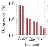
(c)

FIGURE. 1: Descriptive statistics of the OMDB-GAP1 dataset. (a) Distribution of all $12\,500$ band gaps with population statistics: $\text{mean}=3.05$, $\text{median}=2.96$, $\text{standard deviation}=1.03$. The distribution exhibits the form of the Wigner-Dyson distribution with the estimated parameters: $\sim x^{4.61}e^{-0.28x^{2}}$ (b) The most common space groups. (c) The most common elements, excluding C and H, which occur in all the structures.

Organics were reported to contain strongly correlated electrons as well as intermolecular van-der-Waals interactions that usually require the application of advanced exchange-correlations functionals, such as Meta-GGAs or hybrid functionals as well as van-der-Waals interactions Buchholz and Stein (2018); Kronik and Tkatchenko (2014); da Silva et al. (2017). However, to obtain a statistically relevant dataset while keeping a reasonable computational demand, we chose the generalized gradient approximation according to PBE Perdew et al. (1996). The distribution of the calculated band gaps exhibits the form of the Wigner-Dyson distribution ($\sim x^{\alpha}\exp(-\beta\ x^{2})$) and is shown in Figure 1a. Choosing PBE can introduce a systematic error into the calculations (e.g. changing the position of the mean and the size of the variance), however, it does not affect the overall statistical properties of the dataset (shape of the band gap distribution). In particular, the latter is important for the development of machine learning models, which, once they reach chemical accuracy, can be applied to an improved dataset whenever present.

Typically, the computational demand for DFT calculations tremendously increases with the number of atoms $N_{a}$ in the unit cell. Even though implementations with $\mathcal{O}\left(N_{a}\right)$ scaling were reported Guerra et al. (1998); Zeller (2008), commonly used DFT codes scale with $\mathcal{O}\left(N_{a}^{2}\log N_{a}\right)$ up to $\mathcal{O}\left(N_{a}^{3}\right)$ Kresse and Furthmüller (1996b). This represents a serious problem for ab initio modeling of organic crystal structures. Next to the number of atoms, also other parameters like the energy cut-off for the plane-wave expansion influence the computing time. For the present dataset, the calculations were running for $\approx 60$ core hours for an average material, leading to a total estimate of 750k core hours for the entire dataset.

III Results and Discussion

III.1 Machine learning for organic crystals

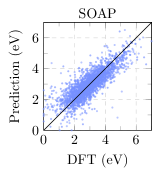
(a)

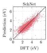
(b)

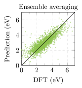
(c)

FIGURE. 2: Band gap predictions for the $2500$ test materials for the models (a) SOAP (MAE $0.430\text{\,}\mathrm{eV}$), (b) SchNet (MAE $0.415\text{\,}\mathrm{eV}$) and the (c) SOAP/SchNet ensemble (MAE $0.388\text{\,}\mathrm{eV}$).

For a prediction of the electronic band gap based on machine learning we discuss two recent models: kernel ridge regression with the SOAP kernel Bartók et al. (2013) and the deep learning model SchNet Schütt et al. (2018a). A brief introduction to both models is given in Appendix A. As an input, we use the atom positions and corresponding atomic numbers. We train the models using $10\,000$ materials (training set) and evaluate their performance using Mean Absolute Error (MAE) and Root Mean Squared Error (RMSE) for the remaining $2500$ materials (test set).

Table 2 and Figure 2 summarize the best performance of each model after hyperparameter optimization (more details given in the appendix). The “Constant” model refers to using the mean (for RMSE) and median (for MAE) values from the training set as the most basic baselines to calculate, respectively. Although SchNet is more accurate (MAE $0.415\text{\,}\mathrm{eV}$) than SOAP (MAE $0.430\text{\,}\mathrm{eV}$), it overestimates the band gap of the metals and small-gap materials (Fig. 2b). For SOAP, the MAE on the training data is $0.342\text{\,}\mathrm{eV}$, indicating that the model is overfitting slightly. In contrast, the MAEs for SchNet on the training and validation set are $0.274\text{\,}\mathrm{eV}$ and $0.397\text{\,}\mathrm{eV}$, respectively. The deep learning model SchNet has more free parameters than SOAP, which makes it more prone to overfitting. The result can be slightly improved by considering an ensemble average prediction Murphy (2012), leading to a MAE of $0.388{}\text{\,}\mathrm{eV}$ and an RMSE of $0.519\text{\,}\mathrm{eV}$, indicating that the errors of both models are slightly uncorrelated. Considering a mean band gap of $3.05\text{\,}\mathrm{eV}$ as shown in Figure 1a, this corresponds to a percentage error of $\approx$$13\text{\,}\mathrm{\char 37\relax}$. Whether this performance is accurate enough to screen for materials and how many complementary computationally expensive DFT calculations are required depends on the application domain. For example, efficiency of solar cells can be estimated using the Shockley-Queisser (SQ) limit for a single p-n junction. For the band gap of $1.34\text{\,}\mathrm{eV}$, it gives the maximum performance corresponding to $33.7\text{\,}\mathrm{\char 37\relax}$. In this case, the MAE of $0.388\text{\,}\mathrm{eV}$ would correspond to $5.1\text{\,}\mathrm{\char 37\relax}$ performance decrease Rühle (2016).

FIGURE. 3: Benchmark of SOAP and SchNet on the OMDB band gap dataset (OMDB-GAP1). SOAP is used with an average kernel and with $r_{c}=$4\text{\,}\mathrm{\SIUnitSymbolAngstrom}$,n=8,l=6$. SchNet is used with $T=3,F=64$ and a validation set of $1000$ materials is used for early stopping.

Table 2: Performance of different models on the test set (complete training set is used for training). The “constant” model corresponds to predicting the median and mean of the training set for MAE and RMSE, respectively.

	MAE (eV)	RMSE (eV)
Constant	0.797	1.035
SOAP	0.430	0.576
SchNet	0.415	0.554
Ensemble averaging	0.388	0.519

FIGURE. 4: Dimensionality-reduced visualization of the crystal structures with the t-SNE algorithm Maaten and Hinton (2008) with perplexity 50. The distance between two structures is determined by the average SOAP kernel ($r_{c}=$4\text{\,}\mathrm{\SIUnitSymbolAngstrom}$,n=8,l=6$). The PBE band gap is color-coded for each structure. Regions with both similar structure and band gap can be recognized. Structures related to chemical hydrogen storage devices appear in the vicinity of (a) OMDB-ID 36754 (C4 H14 B4 N4) and (b) OMDB-ID 22958 (C3 H12 B N). Structures with similar Boron-containing clusters form the island including (c) OMDB-ID 4085 (C12 H34 B12 N4) and (d) OMDB-ID 26557 (C14 H16 B10 F4). Molecular crystals are present in in the region of (e) OMDB-ID 1637 (C21 H10 F6 O4) and (f) OMDB-ID 4532 (C18 H10 Cl2 F5 N O2). A molecular metal (g) OMDB-ID 16923 (C18 H16 Br S8) and a structurally similar organic superconductor (h) OMDB-ID 33839 (C24 H24 F6 P S16) appear in the same zero band gap region. Online interactive version (with zoom) available at https://omdb.mathub.io/dataset/OMDB-GAP1/interactive.

Figure 3 shows the mean absolute error (MAE) decrease with the number of training examples $N$ on a log-log scale, revealing a roughly linear trend. For SOAP and SchNet a power law is fitted to $0.965N^{-0.087}$ and $1.507N^{-0.140}$, respectively. We use this approximation to estimate the number of materials necessary to reach a certain level of predictive power. For example, if we aim for a MAE of $0.1\text{\,}\mathrm{eV}$, which corresponds to a percentage error of $3\text{\,}\mathrm{\char 37\relax}$ on the average band gap of $3.05\text{\,}\mathrm{eV}$, the upper bound for SchNet is approximately 267M materials, which is far beyond the scale of available band gap data for organic molecular crystals (e.g., the COD contains crystallographic information for $\approx$ $325\,000$ organic crystals). As this number is prohibitively large with current computational resources, it indicates the necessity for more powerful machine learning models and/or simplifying assumptions which incorporate domain knowledge to reach this level of accuracy. Meanwhile, the current accuracy can be used to reduce the search space for high-throughput screening with DFT.

The model based on the average SOAP kernel has fewer free parameters than SchNet. Therefore, it is expected that SOAP outperforms SchNet for a small number of training examples, where SchNet is more likely to overfit. However, training of SchNet has linear complexity with the number of training examples, whereas the complexity is cubic for SOAP. In practice, this means SchNet can be trained on a larger set of materials.

To visualize the relationship between the OMDB-GAP1 crystal structures and their band gap, we used the learned SOAP kernel to measure the structural similarity of two materials $A$ and $B$ as $D(A,B)^{2}=K(A,A)+K(B,B)-2K(A,B)$ De et al. (2016). This distance measure is used by a dimensionality reduction algorithm t-SNE Maaten and Hinton (2008) to construct a two-dimensional projection of the high-dimensional crystal structure data. The results shown in Figure 4 exhibit a clear gradient in the band gap size from materials clustered in the upper left corner (large band gap) to materials in the lower right corner (small band gap). We furthermore picked a few examples where we illustrate a selection of crystal structures visualized with the program Mercury Macrae et al. (2006). For example, structures related to chemical hydrogen storage devices appear in the vicinity of each other, such as Bis-BN Cyclohexane (Figs. 4(a) with $4.7\text{\,}\mathrm{wt\%}$ hydrogen storage capabilityChen et al. (2014) and Propylamine–borane (Figs. 4(b). Similarly, crystals with Boron-containing clusters, which have applications in the pharmaceutical industry Leśnikowski (2016), are shown in Figs. 4(c) and (d), and pure molecular crystals can be identified in Figs. 4(e) and (f). The 36 metals present in the OMDB-GAP1 shown in Fig. 4(g) appear close to the structurally similar organic superconductor $\beta\text{-(meso-DMBEDT-TTF)}_{2}\text{PF}_{6}$ (transition temperature $T_{c}=$4.2\text{\,}\mathrm{K}$$ Kimura et al. (2004)) shown in Fig. 4(h).

FIGURE. 5: Principal component analysis (PCA) of the learned embeddings $\bm{a}_{Z}$ ($F=64$-dimensional) in SchNet ($T=1$, 9000 training examples). Elements that occur in fewer than 35 materials are ignored. Groups of the periodic table denoted by CAS numbering can be recognized.

The dimensionality-reduced visualization where the functional property (e.g. band gap) is color-coded provides an intuitive way to navigate the structure-property landscape of organic crystals. With that it provides a basic approach to narrow down the search space to identify materials with a specified target functionality, e.g., materials for hydrogen storage or superconductors. In addition to the previous examples, by zooming in on certain areas it is possible to find structures forming a line that represents a study of the effect of pressure on a crystal structure. Other regions of interest can be explored using the online interactive version at https://omdb.mathub.io/dataset/OMDB-GAP1/interactive, which also provides a zoom functionality.

The way SchNet model calculates its final prediction as an average of individual atomic contribution makes it possible to identify structure-property relationships for separate atoms. The atom embeddings $\bm{a}_{Z}$ (with dimensionality $F$) are initialized randomly and updated while training the network. The learned embeddings can be studied in a dimensionality-reduced picture as well, which shows that SchNet has learned similarity between certain atom types as in the periodic table (Figure 5). Generally speaking, elements that have a similar local environment and contribute similarly towards the final prediction are expected to have similar embeddings, but the exact way chemical information stored in the embeddings while training is non-trivial. We observe that the groups such as VIIA and VIB form clusters. Note that extracting the periodic table from machine learning models is also possible in the case of SOAP with a chemical environment kernel Willatt et al. (2018a). Alternatively, it is also possible to use only compositional information to create atom embeddings that can reconstruct the periodic table Zhou et al. (2018).

III.2 High-throughput screening of the COD Database

The previously trained models are able to make band gap predictions for millions of organic crystal structures and narrow the search space down where computationally expensive conventional methods such as DFT can subsequently be used. As a demonstration, we employ the trained models to calculate the band gap for the materials contained in the Crystallography Open Database (COD). The database contains $399\,020$ Crystallographic Information Files (CIF), of which $307\,013$ are organic (i.e. include C and H) and consist of the 65 elements present in OMDB-GAP1. The COD has an average of $317$ atoms in the unit cell, significantly larger than the average of 82 atoms within our dataset. To eliminate extremely large structures we only consider structures with the maximum of 500 atoms in the unit cell, leading to $260\,092$ structures.

Figure 6 shows the distribution of band gap predictions which is similar to Figure 1a. The COD predictions are available to download from https://omdb.mathub.io/dataset. As a proof of concept, we search for predicted solar cells around the Shockley-Queisser (SQ) limit $1.34\pm 0.05\text{\,}\mathrm{eV}$ of the SOAP/SchNet average ensemble predictions and find 3343 candidate materials (excluding materials present in OMDB-GAP1). This represents $1.3\text{\,}\mathrm{\char 37\relax}$ of the initial search space on which more accurate high-throughput DFT calculations can be used for verification. Table 3 lists a random selection of candidate materials (with $N<200$) for solar cells identified by the SOAP/SchNet average ensemble (i.e. materials with a predicted band gap within the range of $1.34\pm 0.05\text{\,}\mathrm{eV}$. Note that this search does not take the band dispersion into account and whether a band gap is direct or indirect. A more extensive study focused on organic solar cells will be the topic of future work.

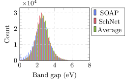
FIGURE. 6: Distribution of $260\,092$ COD band gap predictions. The distribution exhibits the form of the Wigner-Dyson distribution with estimated parameters $\sim x^{5.31}e^{-0.41x^{2}}$, $\sim x^{6.39}e^{-0.51x^{2}}$ and $\sim x^{6.03}e^{-0.48x^{2}}$ for SOAP, SchNet and the ensemble average, respectively.

Table 3: Random selection of 15 candidate materials with $N\leq 200$ for solar cells identified by SOAP/SchNet average ensemble. The predicted band gaps are listed as well as the number of atoms in the unit cell ($N_{a}$) and the space group number (SG).

Compound	N	COD-ID	SG	Band gap (eV)
C34H40Co3N16O8	101	7033509	2	1.387
C32H40Cl8Mn4N16O8	108	7013640	15	1.293
C52H36N20O28	136	7219834	14	1.336
C40H40Cu4F24N8O8W4	128	2006452	14	1.301
C84H60Cu4N12O20	180	2215189	14	1.363
C36H40Cu4I4N20O4	108	7009105	14	1.341
C70H40Cl14N6O6Ru2	138	7027581	2	1.340
C48H32Cu4I4N8	96	2227752	19	1.293
C52H44AlN4O2	103	4331896	2	1.389
C28H32N4Ni2O12	78	2227456	14	1.352
C48H60Ba2N8O32	150	2012449	14	1.356
C94H64Co4N24O6S8	200	2239446	4	1.340
C34H42FeN4NiS6	88	4322934	2	1.346
C56H48N8O14Zn2	128	7229269	2	1.381
C32H32Cl4N8Ni2O8	86	2235069	14	1.318

IV Conclusion

We present the new OMDB-GAP1 dataset which contains DFT bandgaps for $12\,500$ organic crystal structures, which span 69 space groups and 65 elements, to facilitate data-driven approaches in materials science. The structures have on average 82 atoms per unit cell which represents a challenging benchmark for machine learning models comparing to the existing materials datasets. We train two recent machine learning models, kernel ridge regression with the Smooth Overlap of Atomic Positions (SOAP) kernel and the deep learning model SchNet, on this new dataset and find that an ensemble of these two models reaches mean absolute error (MAE) of $0.388\text{\,}\mathrm{eV}$, which corresponds to a percentage error of $13\text{\,}\mathrm{\char 37\relax}$ on the average band gap of $3.05\text{\,}\mathrm{eV}$. Scaling properties of the prediction error with the number of materials used for model training indicate that a prohibitively large number of materials would be required to reach chemical accuracy. It suggests that, for the large crystal structures, machine learning approaches require development of new model architectures which utilize domain knowledge and simplifying assumptions.

The models can also provide chemical insights into the data. For example, by visualizing the SOAP kernel-based similarity between the crystals, different clusters of materials can be identified, such as organic metals or semiconductors. Finally, the trained models are employed to predict the band gap for $260\,092$ materials contained within the Crystallography Open Database (COD) and made available online (see Appendix C) so the predictions can be obtained for any arbitrary crystal structure uploaded by a user.

Data Availability

The datasets are available from https://omdb.mathub.io/dataset, including both the OMDB-GAP1 dataset and the COD predictions. To facilitate the training of the SchNet model on this dataset, our preprocessing script is available in the official SchNetpack repository at https://github.com/atomistic-machine-learning/schnetpack/tree/master/src/scripts/schnetpack_omdb.py.

Author Contributions

All authors designed the study. B.O., S.S.B. and R.M.G. prepared the dataset and performed the machine learning study. R.M.G. performed the DFT calculations. All authors analyzed the results, wrote, and revised the manuscript.

Competing Interests

The authors declare no competing interests.

Appendix A Machine Learning Models

From a machine learning point of view, band gap prediction represents a regression task, which aims to find a non-linear relation $y=f(\bm{x})$ between an input vector $\bm{x}$ (commonly referred to as “features”) and an output $y$ (commonly referred to as “target”). The information about a molecule or crystal structure is usually represented as atomic positions and atomic numbers. A common strategy is to construct a descriptor $\bm{x}$ that encodes this information in a fixed-size vector. Depending on the context in which the descriptors are used, certain properties such as translation, rotational, atom index invariance and differentiability are important Rupp et al. (2012); Faber et al. (2015). This task is difficult since equivalent crystal structures can easily lead to distinct representations, causing inconsistent data for numerical methods. Many different descriptors have been introduced in the literature, such as the Coulomb matrix Rupp et al. (2012), Bag-of-Bonds Hansen et al. (2015), Sine Matrix Faber et al. (2015) and MBTR Huo and Rupp (2017). An alternative strategy is to skip the intermediate step of fixed-size descriptors, which often involve ad-hoc decisions, and directly define the kernel between two structures as in the Smooth Overlap of Atomic Positions (SOAP) kernel, which has shown superior performance on a variety of problems De et al. (2016); Jäger et al. (2018).

In this paper, two recent machine learning models are evaluated on the new dataset: SOAP Bartók et al. (2013) and SchNet Schütt et al. (2018a). This provides a baseline estimate of the predictive power of current models for the presented dataset. In this study, the atomic numbers and positions are available, but there exist alternative approaches if only the composition of a crystal is known, such as the automatically generated features from Magpie Ward et al. (2016).

The models studied here can be used for a fast screening of desired material properties, after which traditional calculations can be used to verify the results. Additionally, the considered models are differentiable with respect to atom positions, which means that the output property can be tuned through gradient descent. When a model is trained to predict total energy, the differentiability provides forces that enable geometry optimization of large structures or simulate dynamics on longer timescales than traditionally feasible Schütt et al. (2018a).

To train the models in this work, we use the first $10\,000$ structures as the training dataset and the last $2500$ structures to calculate the out-of-sample predictive performance. Finally, as negative gaps are unphysical, the models’ predictions are clipped to zero, i.e. $\hat{y}=\max(0,f(\bm{x}))$.

A.1 Kernel Ridge Regression with SOAP

Kernel ridge regression (KRR) has been used for a variety of studies involving quantum-mechanical calculations Rupp et al. (2012); Rupp (2015); Faber et al. (2015); De et al. (2016); Huo and Rupp (2017); Jäger et al. (2018).

KRR is based on linear ridge regression for the features $\bm{x}\in\mathcal{X}$ transformed to a higher-dimensional space $\mathcal{Z}$. It turns out that it is possible to perform ridge regression on the transformed datapoints $\bm{z}_{i}=\phi(\bm{x}_{i})$ without explicitly converting the points by using the so-called kernel trick. This is achieved by defining a kernel that corresponds to an inner product in $\mathcal{Z}$, i.e. $k(\bm{x},\bm{x^{\prime}})=\left<\phi(\bm{x}),\phi(\bm{x}^{\prime})\right>$. For a derivation of KRR see Murphy (2012).

KRR introduces one constant parameter in the model that has to be chosen before training, i.e. a hyperparameter. This is the regularization coefficient $\lambda$. In this paper, it is optimized using a grid search within 10-fold cross validation (see Appendix for details).

The goal of the SOAP kernel is to provide a measure of similarity between two structures, i.e. a structural similarity kernel Bartók et al. (2013); De et al. (2016). In practice, this is a two-step process. First, a measure of similarity between two local environments $\mathcal{X}$ and $\mathcal{X^{\prime}}$ is defined. Second, these local environment kernels are combined into a global similarity kernel. The local environment of an atom is constructed by placing a Gaussian at each neighboring atom position. The similarity (or overlap) between two environments $K(\mathcal{X},\mathcal{X}^{\prime})$ is calculated by integrating the overlap under all SO(3) rotations. For more details on SOAP see Bartók et al. (2013); Willatt et al. (2018b).

The local environment kernels also depend on a number of hyperparameters. The most important is the cut-off distance $r_{c}$ that determines the radius of the environments considered. Additionally, the integration is in practice performed by expanding the environments in spherical and radial basis functions. This gives two additional hyperparameters, the number of radial basis functions $n$ and the maximum degree $l$ of the spherical harmonics. Figure 7 and Table 4 in the appendix show the performance for a number of different choices of $r_{c}$. The parameters $n=8$ and $l=6$ are chosen sufficiently high as was shown in Bartók et al. (2013).

There are several ways local environment kernels can be combined into a global similarity kernel. Two common choices are the fast average kernel and the “regularized-entropy match” (RE-Match) kernel De et al. (2016). The fast average kernel corresponds to taking the average of all pair-wise environment kernels, whereas the RE-Match kernel is based on finding the best matches for each atomic environment De et al. (2016). However, the RE-Match scheme is prohibitively slow and memory-consuming in its current implementations for the presented dataset. Hence, the fast average kernel is used, which implementation is available at https://github.com/cosmo-epfl/glosim.

A.2 SchNet

The SchNet model is a deep learning architecture based on artificial neural networks that is designed to work with both molecules and crystal structures Schütt et al. (2018a). This deep learning model is “end-to-end” and does not require hand-crafted descriptors of the input data. Its architecture is inspired by the success of convolutional neural networks applied to image and video data. Other similar models include the HIP-NN Lubbers et al. (2018) and the crystal graph convolutional networks Xie and Grossman (2018).

In contrast to images, atomic positions cannot be efficiently represented using a simple uniform grid structure. Additionally, images usually have a fixed number of pixels whereas crystals can contain varying number of atoms. These issues are resolved by using the weight-sharing approach, which is common in both convolutional and recurrent neural networks. It assumes that the same network is used for each individual atom leading to an atom-wise contribution to the final prediction. The total number of contributions for a crystal structure is equal to the total number of atoms, and the final prediction is obtained by either averaging or summing all the contributions, referred to as “pooling”. The pooling procedure maintains the atom index invariance because summing or averaging the atomic contributions is communicative. In practice, this means that SchNet decomposes a property into individual atomic contributions. For intensive properties, the mean of the atom contributions is taken, otherwise the sum is used. Besides introducing atom index invariance, it makes the model partially interpretable, since the final prediction can be explained by these individual contributions.

The SchNet architecture consists of four building blocks: atom embedding, atom-wise layers, interaction blocks and filter-generating networks. First, atoms are represented (embedded) by a vector $\bm{a}_{Z}\in\mathbb{R}^{F}$ depending on the proton number $Z$. $F$ is the dimensionality of the atom embedding. Interactions with neighbouring atoms (including periodic boundary conditions) are introduced by the interaction blocks. Here, a cut-off for the environments considered is used, which we take as $5\text{\,}\mathrm{\SIUnitSymbolAngstrom}$ as in the original paper. The contributions by neighbouring environments in the interaction blocks are mediated by atom-wise layers and filter-generating networks. The computational details of these components are beyond the scope of this article but are available in Schütt et al. (2018a, b).

The embeddings and atom-wise layers are optimized for the target property $y$ using a gradient descent method on the squared loss function $\min\limits_{\theta}L(\theta)=||y-\hat{y}||^{2}$, where $\theta$ are parameters of the network. Similar to Schütt et al. (2018b), we reduce the learning rate $\eta=0.001$ with a decay factor of $0.6$, and use the ADAM optimizer Kingma and Ba (2014). We train SchNet with a batch size of $32$ and use a validation set of $1000$ examples for early stopping or as long as $\eta^{\prime}>\eta/10$. The latest implementation of SchNet in SchNetPack is used here, available at https://github.com/atomistic-machine-learning/schnetpack. We use two NVIDIA Tesla K80 for training.

Besides the standard training hyperparameters such as learning rate $\eta$ and batch size, there are a number of hyperparameters specific to SchNet. First, the cut-off radius $r_{c}$ is set to $5\text{\,}\mathrm{\SIUnitSymbolAngstrom}$, which was demonstrated to lead to accurate results on bulk crystal structures from the Materials Project Schütt et al. (2018a). Second, the dimensionality of the embeddings $F$ is set to 64. Finally, the number of interaction blocks $T$ is varied between 3 and 6 (see Appendix B and Figure 8 for more details).

Appendix B Hyperparameter optimization

The machine learning models used for band gap prediction in this work, SOAP and SchNet, include parameters that have to be chosen before training begins, referred to as hyperparameters. The two models have different hyperparameters which are discussed separately in this appendix.

B.1 SOAP

The Smooth Overlap of Atomic Positions kernel relies on several hyperparameters. First, an environment $\rho$ (i.e. a set of neighboring atoms) is constructed by placing a single Gaussian on each neighboring atom position. The kernel $k(A,B)$ is calculated for two different environments A and B as the overlap of $\rho_{A}$ and $\rho_{B}$ while also integrating over all possible rotations Bartók et al. (2013). The number of radial $n$ and the maximum degree of spherical harmonics $l$, determine the precision with which the overlap integral is performed. These parameters are set to $n=8,l=6$ as this was shown to lead to accurate results Bartók et al. (2013). Finally, the most important hyperparameter is the cut-off radius $r_{c}$ that determines the cut-off radius for the local environments, i.e. which neighboring atom positions are included in the overlap integral. Figure 7 shows the performance of SOAP for varying cut-off radii $r_{c}$. The lowest mean absolute error (MAE) is obtained for $r_{c}=$4\text{\,}\mathrm{a}\mathrm{n}\mathrm{g}\mathrm{s}\mathrm{t}\mathrm{r}\mathrm{o}\mathrm{m}$$.

FIGURE. 7: Performance of SOAP (average global kernel with $n=8$ and $l=6$) on the OMDB band gap dataset (OMDB-GAP1).

Table 4 summarizes the performance of varying $r_{c}$ with all $10\,000$ training examples.

Table 4: Summary of SOAP (with average kernel $n=8$ and $l=6$) performance with $10\,000$ training examples.

$r_{c}$ (Å)	MAE (eV)	RMSE (eV)
3	0.431	0.582
4	0.430	0.576
5	0.437	0.594
6	0.445	0.601

B.2 SchNet

The SchNet model is an artificial neural network that consists of four different components: atom embeddings, atom-wise layers, interaction blocks and filter-generating networks. See Schütt et al. (2018a) for a schematic drawing of the model and its components. The interactions with neighboring atoms (including periodic boundary conditions) are included through interaction blocks that rely on filter generators. Increasing the number interaction blocks $T$ in the model increases the depth of the model and the number of parameters $\theta$. For example, a model with $F=64$ and $T=3$ has $63\,333$ parameters, whereas a model with $T=6$ has $117\,953$ parameters. $T$ is a hyperparameter to be set before training. SchNet is evaluated on each site in the crystal structure and the final band gap prediction is the mean of the atom-wise contributions. Figure 8 show the performance of SchNet for a varying number of interactions blocks $T$ and training examples. Table 5 summerizes the results with the maximum number of 9000 training examples (the remaining 1000 validation examples are used for model selection).

FIGURE. 8: Benchmark of SchNet on the OMDB band gap dataset (OMDB-GAP1). $F=64$,$r_{c}=$5\text{\,}\mathrm{\SIUnitSymbolAngstrom}$$

Table 5: Summary of SchNet performance with $9000$ training examples with $1000$ validation examples for model selection (early stopping), $F=64$, $r_{c}=$5\text{\,}\mathrm{\SIUnitSymbolAngstrom}$$.

$T$	MAE (eV)	RMSE (eV)
1	0.431	0.584
3	0.415	0.554
6	0.419	0.565

Figure 9 shows the training and validation loss during the training of SchNet (with $T=3$). After many epochs, SchNet is able to overfit to the training data completely due to its many free parameters. The validation loss is used to select the best model, which in this case occurs at epoch 44.

FIGURE. 9: The training and validation loss while training SchNet with 9000 training examples and $T=3$.

FIGURE. 10: The trained models are available through a web interface at https://omdb.mathub.io/ml.

Appendix C Web interface

We implemented a web interface that can predict band gap properties for a user-uploaded Crystallographic Information File (CIF) containing the crystal structure (Figure 10). The trained models scale differently when presented a new crystal structure. SchNet is a parametric model with a fixed number of parameters per atom that is evaluated on each site. Therefore, it scales linearly with the the number of atoms in the unit cell Schütt et al. (2018a). Kernel ridge regression, on the other hand, scales with the number of training samples $N$ because it requires calculating the kernel-based similarity between the new structure $A$ and all the reference examples $B_{i}$ in the training set to make a prediction of the target property $g$, i.e. $g=\sum_{i}^{N}\alpha_{i}K(A,B_{i})$, where $\alpha_{i}$ are the regression coefficients. It takes $\approx$ 10 seconds for SchNet and $\approx$ 1 minute for SOAP to calculate the prediction using the online interface.

References

- Downs and Hall-Wallace (2003) R. T. Downs and M. Hall-Wallace, “The american mineralogist crystal structure database,” American Mineralogist 88, 247–250 (2003).
- Merkys et al. (2016) Andrius Merkys, Antanas Vaitkus, Justas Butkus, Mykolas Okulič-Kazarinas, Visvaldas Kairys, and Saulius Gražulis, “COD::CIF::Parser: an error-correcting CIF parser for the Perl language,” Journal of Applied Crystallography 49 (2016), 10.1107/S1600576715022396.
- Groom et al. (2016) Colin R. Groom, Ian J. Bruno, Matthew P. Lightfoot, and Suzanna C. Ward, “The Cambridge Structural Database,” Acta Crystallographica Section B 72, 171–179 (2016).
- Bergerhoff et al. (1987) G Bergerhoff, ID Brown, F Allen, et al., “Crystallographic databases,” International Union of Crystallography, Chester 360, 77–95 (1987).
- Jain et al. (2013) Anubhav Jain, Shyue Ping Ong, Geoffroy Hautier, Wei Chen, William Davidson Richards, Stephen Dacek, Shreyas Cholia, Dan Gunter, David Skinner, Gerbrand Ceder, and Kristin a. Persson, “The Materials Project: A materials genome approach to accelerating materials innovation,” APL Materials 1, 011002 (2013).
- Borysov et al. (2017) Stanislav S. Borysov, R. Matthias Geilhufe, and Alexander V. Balatsky, “Organic materials database: An open-access online database for data mining,” PLOS ONE 12, e0171501 (2017).
- Draxl and Scheffler (2018) Claudia Draxl and Matthias Scheffler, “Nomad: The fair concept for big-data-driven materials science,” arXiv preprint arXiv:1805.05039 (2018).
- Ortiz et al. (2009) C. Ortiz, O. Eriksson, and M. Klintenberg, “Data mining and accelerated electronic structure theory as a tool in the search for new functional materials,” Computational Materials Science 44, 1042 – 1049 (2009).
- Nakata and Shimazaki (2017) Maho Nakata and Tomomi Shimazaki, “Pubchemqc project: A large-scale first-principles electronic structure database for data-driven chemistry,” Journal of chemical information and modeling 57, 1300–1308 (2017).
- Wishart et al. (2017) David S Wishart, Yannick D Feunang, An C Guo, Elvis J Lo, Ana Marcu, Jason R Grant, Tanvir Sajed, Daniel Johnson, Carin Li, Zinat Sayeeda, et al., “Drugbank 5.0: a major update to the drugbank database for 2018,” Nucleic acids research 46, D1074–D1082 (2017).
- Schomburg et al. (2002) Ida Schomburg, Antje Chang, Oliver Hofmann, Christian Ebeling, Frank Ehrentreich, and Dietmar Schomburg, “Brenda: a resource for enzyme data and metabolic information,” (2002).
- sup (2011) “National Institute of Materials Science, Materials Information Station, SuperCon ,” http://supercon.nims.go.jp/index_en.html (2011), [Online; accessed September-2018].
- Wimbush and Strickland (2017) Stuart C Wimbush and Nicholas M Strickland, “A public database of high-temperature superconductor critical current data,” IEEE Transactions on Applied Superconductivity 27, 1–5 (2017).
- Borysov et al. (2018) Stanislav S Borysov, Bart Olsthoorn, M Berk Gedik, R Matthias Geilhufe, and Alexander V Balatsky, “Online search tool for graphical patterns in electronic band structures,” Npj Computational Materials 4, 46 (2018).
- Geilhufe et al. (2018) R Matthias Geilhufe, Stanislav S Borysov, Dmytro Kalpakchi, and Alexander V Balatsky, “Towards novel organic high-t c superconductors: Data mining using density of states similarity search,” Physical Review Materials 2, 024802 (2018).
- Suram et al. (2015) Santosh K. Suram, Joel A. Haber, Jian Jin, and John M. Gregoire, “Generating information-rich high-throughput experimental materials genomes using functional clustering via multitree genetic programming and information theory,” ACS Combinatorial Science 17, 224–233 (2015).
- Gilmer et al. (2017) Justin Gilmer, Samuel S. Schoenholz, Patrick F. Riley, Oriol Vinyals, and George E. Dahl, “Neural message passing for quantum chemistry,” in Proceedings of the 34th International Conference on Machine Learning, Proceedings of Machine Learning Research, Vol. 70, edited by Doina Precup and Yee Whye Teh (PMLR, International Convention Centre, Sydney, Australia, 2017) pp. 1263–1272.
- Schütt et al. (2017) Kristof T. Schütt, Farhad Arbabzadah, Stefan Chmiela, Klaus R. Müller, and Alexandre Tkatchenko, “Quantum-chemical insights from deep tensor neural networks,” Nature Communications 8, 13890 (2017).
- Brockherde et al. (2017) Felix Brockherde, Leslie Vogt, Li Li, Mark E. Tuckerman, Kieron Burke, and Klaus-Robert Müller, “Bypassing the kohn-sham equations with machine learning,” Nature Communications 8 (2017), 10.1038/s41467-017-00839-3.
- Stanev et al. (2018) Valentin Stanev, Corey Oses, A. Gilad Kusne, Efrain Rodriguez, Johnpierre Paglione, Stefano Curtarolo, and Ichiro Takeuchi, “Machine learning modeling of superconducting critical temperature,” npj Computational Materials 4 (2018), 10.1038/s41524-018-0085-8.
- De et al. (2016) Sandip De, Albert P. Bartók, Gábor Csányi, and Michele Ceriotti, “Comparing molecules and solids across structural and alchemical space,” Physical Chemistry Chemical Physics 18, 13754–13769 (2016).
- Schütt et al. (2018a) K. T. Schütt, H. E. Sauceda, P.-J. Kindermans, A. Tkatchenko, and K.-R. Müller, “SchNet – a deep learning architecture for molecules and materials,” The Journal of Chemical Physics 148, 241722 (2018a).
- Xie and Grossman (2018) Tian Xie and Jeffrey C. Grossman, “Crystal graph convolutional neural networks for an accurate and interpretable prediction of material properties,” Phys. Rev. Lett. 120, 145301 (2018).
- Rupp et al. (2012) Matthias Rupp, Alexandre Tkatchenko, Klaus-Robert Müller, and O. Anatole von Lilienfeld, “Fast and accurate modeling of molecular atomization energies with machine learning,” Phys. Rev. Lett. 108, 058301 (2012).
- Hansen et al. (2015) Katja Hansen, Franziska Biegler, Raghunathan Ramakrishnan, Wiktor Pronobis, O. Anatole von Lilienfeld, Klaus-Robert Müller, and Alexandre Tkatchenko, “Machine learning predictions of molecular properties: Accurate many-body potentials and nonlocality in chemical space,” The Journal of Physical Chemistry Letters 6, 2326–2331 (2015).
- Faber et al. (2015) F. Faber, A. Lindmaa, O. Anatole von Lilienfeld, and R. Armiento, “Crystal Structure Representations for Machine Learning Models of Formation Energies,” ArXiv e-prints (2015), arXiv:1503.07406 [physics.chem-ph] .
- Huo and Rupp (2017) Haoyan Huo and Matthias Rupp, “Unified representation of molecules and crystals for machine learning,” (2017), arXiv:1704.06439 .
- Vardeny (2009) Valy Vardeny, “Spintronics: Organics strike back,” Nature materials 8, 91 (2009).
- Dediu et al. (2002) V. Dediu, M. Murgia, F.C. Matacotta, C. Taliani, and S. Barbanera, “Room temperature spin polarized injection in organic semiconductor,” Solid State Communications 122, 181 – 184 (2002).
- Chilcote et al. (2018) Michael Chilcote, Yu Lu, Ezekiel Johnston-Halperin, et al., Volume 4: Spin in Organics (World Scientific, 2018).
- Liu et al. (2018) Haoliang Liu, Chuang Zhang, Hans Malissa, Matthew Groesbeck, Marzieh Kavand, Ryan McLaughlin, Shirin Jamali, Jingjun Hao, Dali Sun, Royce A Davidson, et al., “Organic-based magnon spintronics,” Nature materials , 1 (2018).
- Schlegel et al. (2008) C. Schlegel, J. van Slageren, M. Manoli, E. K. Brechin, and M. Dressel, “Direct observation of quantum coherence in single-molecule magnets,” Phys. Rev. Lett. 101, 147203 (2008).
- Lehmann et al. (2007) Joerg Lehmann, Alejandro Gaita-Arino, Eugenio Coronado, and Daniel Loss, “Spin qubits with electrically gated polyoxometalate molecules,” Nature Nanotechnology 2, 312 (2007).
- Pustogow et al. (2018) Andrej Pustogow, Mathias Bories, Anja Löhle, Roland Rösslhuber, Elena Zhukova, Boris Gorshunov, Silvia Tomić, John A Schlueter, Ralph Hübner, Takaaki Hiramatsu, et al., “Quantum spin liquids unveil the genuine mott state,” Nature materials , 1 (2018).
- Lee and Lee (2005) Sung-Sik Lee and Patrick A Lee, “U (1) gauge theory of the hubbard model: spin liquid states and possible application to -(bedt- ttf) 2 cu 2 (cn) 3,” Physical review letters 95, 036403 (2005).
- Shimizu et al. (2003) Y. Shimizu, K. Miyagawa, K. Kanoda, M. Maesato, and G. Saito, “Spin liquid state in an organic mott insulator with a triangular lattice,” Phys. Rev. Lett. 91, 107001 (2003).
- Mesta et al. (2013) Murat Mesta, Marco Carvelli, Rein J De Vries, Harm Van Eersel, Jeroen JM Van Der Holst, Matthias Schober, Mauro Furno, Björn Lüssem, Karl Leo, Peter Loebl, et al., “Molecular-scale simulation of electroluminescence in a multilayer white organic light-emitting diode,” Nature materials 12, 652 (2013).
- Baran et al. (2017) Derya Baran, Raja Shahid Ashraf, David A Hanifi, Maged Abdelsamie, Nicola Gasparini, Jason A Röhr, Sarah Holliday, Andrew Wadsworth, Sarah Lockett, Marios Neophytou, et al., “Reducing the efficiency–stability–cost gap of organic photovoltaics with highly efficient and stable small molecule acceptor ternary solar cells,” Nature materials 16, 363 (2017).
- Bartók et al. (2013) Albert P. Bartók, Risi Kondor, and Gábor Csányi, “On representing chemical environments,” Phys. Rev. B 87, 184115 (2013).
- Ruddigkeit et al. (2012) Lars Ruddigkeit, Ruud van Deursen, Lorenz C. Blum, and Jean-Louis Reymond, “Enumeration of 166 billion organic small molecules in the chemical universe database GDB-17,” Journal of Chemical Information and Modeling 52, 2864–2875 (2012).
- Ramakrishnan et al. (2014) Raghunathan Ramakrishnan, Pavlo O Dral, Matthias Rupp, and O Anatole von Lilienfeld, “Quantum chemistry structures and properties of 134 kilo molecules,” Scientific Data 1 (2014).
- Kresse and Furthmüller (1996a) Georg Kresse and Jürgen Furthmüller, “Efficient iterative schemes for ab initio total-energy calculations using a plane-wave basis set,” Physical Review B 54, 11169 (1996a).
- Kresse and Joubert (1999) Georg Kresse and D Joubert, “From ultrasoft pseudopotentials to the projector augmented-wave method,” Physical Review B 59, 1758 (1999).
- Buchholz and Stein (2018) Hannes Konrad Buchholz and Matthias Stein, “Accurate lattice energies of organic molecular crystals from periodic turbomole calculations,” Journal of Computational Chemistry 39, 1335–1343 (2018).
- Kronik and Tkatchenko (2014) Leeor Kronik and Alexandre Tkatchenko, “Understanding molecular crystals with dispersion-inclusive density functional theory: pairwise corrections and beyond,” Accounts of chemical research 47, 3208–3216 (2014).
- da Silva et al. (2017) Pedro S. Pereira da Silva, Pablo Martín-Ramos, Sérgio R. Domingos, Maria do Carmo Bota de Sousa, Cláudia T. Arranja, Abílio J. F. N. Sobral, and Manuela Ramos Silva, “On the performance of hybrid functionals for non-linear optical properties and electronic excitations in chiral molecular crystals: The case of butterfly-shaped dicinnamalacetone,” ChemPhysChem 19, 82–92 (2017).
- Perdew et al. (1996) John P Perdew, Kieron Burke, and Matthias Ernzerhof, “Generalized gradient approximation made simple,” Physical review letters 77, 3865 (1996).
- Guerra et al. (1998) C Fonseca Guerra, JG Snijders, G t te Velde, and EJ Baerends, “Towards an order-n dft method,” Theoretical Chemistry Accounts 99, 391–403 (1998).
- Zeller (2008) Rudolf Zeller, “Towards a linear-scaling algorithm for electronic structure calculations with the tight-binding korringa–kohn–rostoker green function method,” Journal of Physics: Condensed Matter 20, 294215 (2008).
- Kresse and Furthmüller (1996b) Georg Kresse and Jürgen Furthmüller, “Efficiency of ab-initio total energy calculations for metals and semiconductors using a plane-wave basis set,” Computational materials science 6, 15–50 (1996b).
- Murphy (2012) Kevin Murphy, Machine learning : a probabilistic perspective (MIT Press, Cambridge, Mass, 2012).
- Rühle (2016) Sven Rühle, “Tabulated values of the shockley–queisser limit for single junction solar cells,” Solar Energy 130, 139–147 (2016).
- Maaten and Hinton (2008) Laurens van der Maaten and Geoffrey Hinton, “Visualizing data using t-sne,” Journal of machine learning research 9, 2579–2605 (2008).
- Macrae et al. (2006) Clare F. Macrae, Paul R. Edgington, Patrick McCabe, Elna Pidcock, Greg P. Shields, Robin Taylor, Matthew Towler, and Jacco van de Streek, “Mercury: visualization and analysis of crystal structures,” Journal of Applied Crystallography 39, 453–457 (2006).
- Chen et al. (2014) Gang Chen, Lev N. Zakharov, Mark E. Bowden, Abhijeet J. Karkamkar, Sean M. Whittemore, Edward B. Garner, Tanya C. Mikulas, David A. Dixon, Tom Autrey, and Shih-Yuan Liu, “Bis-BN cyclohexane: A remarkably kinetically stable chemical hydrogen storage material,” Journal of the American Chemical Society 137, 134–137 (2014).
- Leśnikowski (2016) Zbigniew J. Leśnikowski, “Challenges and opportunities for the application of boron clusters in drug design,” Journal of Medicinal Chemistry 59, 7738–7758 (2016).
- Kimura et al. (2004) Shinya Kimura, Tomoko Maejima, Hideaki Suzuki, Ryoma Chiba, Hatsumi Mori, Tadashi Kawamoto, Takehiko Mori, Hiroshi Moriyama, Yutaka Nishio, and Koji Kajita, “A new organic superconductor β-(meso-dmbedt-ttf)2pf6,” Chem. Commun. , 2454–2455 (2004).
- Willatt et al. (2018a) M. J. Willatt, F. Musil, and M. Ceriotti, “A Data-Driven Construction of the Periodic Table of the Elements,” ArXiv e-prints (2018a), arXiv:1807.00236 [physics.chem-ph] .
- Zhou et al. (2018) Quan Zhou, Peizhe Tang, Shenxiu Liu, Jinbo Pan, Qimin Yan, and Shou-Cheng Zhang, “Learning atoms for materials discovery,” Proceedings of the National Academy of Sciences (2018), 10.1073/pnas.1801181115.
- Jäger et al. (2018) Marc O. J. Jäger, Eiaki V. Morooka, Filippo Federici Canova, Lauri Himanen, and Adam S. Foster, “Machine learning hydrogen adsorption on nanoclusters through structural descriptors,” npj Computational Materials 4 (2018), 10.1038/s41524-018-0096-5.
- Ward et al. (2016) Logan Ward, Ankit Agrawal, Alok Choudhary, and Christopher Wolverton, “A general-purpose machine learning framework for predicting properties of inorganic materials,” npj Computational Materials 2 (2016), 10.1038/npjcompumats.2016.28.
- Rupp (2015) Matthias Rupp, “Machine learning for quantum mechanics in a nutshell,” International Journal of Quantum Chemistry 115, 1058–1073 (2015).
- Willatt et al. (2018b) M. J. Willatt, F. Musil, and M. Ceriotti, “Theory and Practice of Atom-Density Representations for Machine Learning,” ArXiv e-prints (2018b), arXiv:1807.00408 [physics.chem-ph] .
- Lubbers et al. (2018) Nicholas Lubbers, Justin S. Smith, and Kipton Barros, “Hierarchical modeling of molecular energies using a deep neural network,” The Journal of Chemical Physics 148, 241715 (2018).
- Schütt et al. (2018b) K. T. Schütt, P. Kessel, M. Gastegger, K. A. Nicoli, A. Tkatchenko, and K.-R. Müller, “SchNetPack: A deep learning toolbox for atomistic systems,” Journal of Chemical Theory and Computation 15, 448–455 (2018b).
- Kingma and Ba (2014) Diederik P. Kingma and Jimmy Ba, “Adam: A method for stochastic optimization,” CoRR abs/1412.6980 (2014), arXiv:1412.6980 .