Charge polarization, local electroneutrality breakdown and eddy formation due to electroosmosis in varying-section channels

Abstract

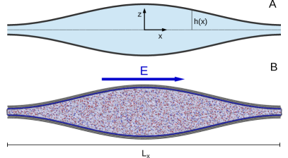
We characterize the dynamics of an electrolyte embedded in a varying-section channel under the action of a constant external electrostatic field. By means of molecular dynamics simulations we determine the stationary density, charge and velocity profiles of the electrolyte. Our results show that when the Debye length is comparable to the width of the channel bottlenecks a concentration polarization along with two eddies sets inside the channel. Interestingly, upon increasing the external field, local electroneutrality breaks down and charge polarization sets leading to the onset of net dipolar field. This novel scenario, that cannot be captured by the standard approaches based on local electroneutrality, opens the route for the realization of novel micro and nano-fluidic devices.

The transport of ions, molecules and polymers across constrictions such as pores, membranes or varying-section micro- nano-channels is crucial for several biological as well as synthetic systems. For example, in biological cells ion channels control the uptake of ions from the environment Hille (2001) whereas, in resistive pulse sensing techniques, the interactions of colloidal particles Weatherall and Willmott (2015) or macromolecules Bayley et al. (2000); Celaya et al. (2017); Bonome et al. (2015); Asandei et al. (2017); Chinappi and Cecconi (2018) with the nano- or micro-pore are measured from the variation of the electric conductance of the pore induced by the presence of the particle. Moreover, electro-osmotic flux can play a crucial role in molecule capturing in nanopores Asandei et al. (2016); Boukhet et al. (2016); Huang et al. (2017). Recent studies have shown that ionic transport and electro-osmotic flow in micro- and nano-fluidic circuitry can be controlled by tuning the geometry of the micro- nano-channelMalgaretti et al. (2015, 2016); Bolet et al. (2018). Indeed, conical Guo et al. (2013); Balme et al. (2017); Experton et al. (2017) or heterogeneously charged Picallo et al. (2013) pores have been used to realize nano-fluidic diodes and to rectify electro-osmotic flows Laohakunakorn and Keyser (2015); Bacchin (2018). Moreover, periodic varying-section channels have been used to realize nanofluidic transistors Kalman et al. (2008). Similarly, recent contributions have shown that the shape of the confining vessel and the boundary conditions therein imposed can be exploited to control the flow. Indeed, electro-osmotic transport can be strongly enhanced by grafting charged brushes on the channel walls Chen and Das (2017) and by hydrophobic surfaces Maduar et al. (2015).

Figure 1: System set-up. A) Sketch of the system. The electrolyte solution (light blue) is confined between two curved charged walls. Half section is $h(x)=h_{0}+h_{1}\cos{\frac{2\pi x}{L_{x}}}$. Periodic boundary conditions are applied in the x and y direction. B) Snapshot of molecular dynamics set-up. The solid walls (gray) are constituted by Lennard-Jones atoms. The atoms of the layer exposed to the liquid are charged (blue). Water molecules are not reported while blue and red spheres represent $K^{+}$ and $Cl^{-}$ ions. An external electrical field parallel to the x-axes in applied.

Figure 2: Net concentration of $Cl^{-}$ and velocity profile (arrows) for external fields corresponding to potential drop $\Delta V=0.6$ (left) and $\Delta V=2.4$ V, (right). Panels a), b) (first row) refer to ion concentration $\rho_{0}=3$M, panels c), d) (central row) refer to $\rho_{0}=1$M and panels e), f) (bottom row) refer to $\rho_{0}=0.3$M. For clarity sake, the arrows of the velocity profile are rescaled in each panel. The upper and bottom Grey solid lines indicates the channel walls.

In this contribution, we study, via molecular dynamics simulations the electro-osmotic flow of an electrolyte embedded in a varying-section channel. The advantage of our approach, as compared to others based on the solution of some continuum models Rubinstein and Zaltzman (2000); Park et al. (2006); Mani et al. (2009); Mani and Bazant (2011); Green et al. (2014), is that the ionic densities are left free to relax according to the interactions among ions and between ions and the channel walls. Therefore our approach allows us to critically discuss, for example, the local electroneutrality assumption and its possible breakdown. Our results show that when the systems is driven by a constant electrostatic field acting along the longitudinal axis of the channel, inhomogeneous ionic and charge densities are induced due to the variations of local channel section. This phenomenon is similar to concentration polarization (CP) reported for electrolytes transported across ionic-selective membranes Rubinstein and Zaltzman (2000); Mani et al. (2009); Zangle et al. (2009) (see also Ref. Chang et al. (2012); Nikonenko et al. (2014) for recent reviews) i.e., in open circuit conditions and under severe modulations of channel section Mani et al. (2009); Zangle et al. (2009); Green et al. (2014). Interestingly, our results show that CP can be obtained also for close circuit conditions and for smooth variations of channel section. In particular, we observe CP when the Debye length is comparable with the channel bottlenecks, i.e., in the entropic electrokinetic regime Malgaretti et al. (2014). Concerning local electroneutrality, our numerical results confirm that even in the entropic electrokinetic regime, the local electroneutrality assumed by previous works Mani and Bazant (2011); Nikonenko et al. (2014); Green et al. (2014); Leese and Mattia (2014) is fulfilled for mild values of the external field. However, upon increasing the external field our numerical simulations show that local electroneutrality breaks down and charge polarization (QP) sets, leading to the onset of a net dipolar contribution to the electrostatic field. Interestingly, a similar phenomenon has been recently observed for pressure-driven flows across conical pores Jubin et al. (2018).

Results

We study the electro-osmotic flow (see Suppl. Mat. for the details) of a KCl water solution across a channel with half section

$$h(x)=h_{0}+h_{1}\cos(2\pi x/L_{x})$$ (1)

with average section $h_{0}=38.5$Å  and modulation $h_{1}=32.5$Å  and periodicity $L_{x}=836.6$Å, see Fig. 1. Channel section is constant along the $y$ direction, with thickness $L_{y}=60.37$Å, and periodic boundary conditions are applied along $x$ and $y$. Both channel walls are covered with a constant charge density $\sigma=0.15\frac{C}{m^{2}}$. The system is globally electroneutral since we compensated the wall charge with additional $Cl^{-}$ ions. After equilibration, a homogeneous and constant external electric field ${\bf E}=(E_{x},0,0)$ is applied to the whole system.

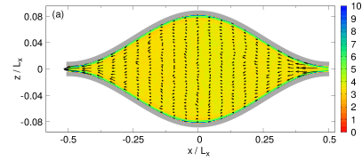
We begin our analysis by focusing on the case of larger ionic concentration $\rho_{0}\simeq 3M$. The density profile of both $Cl^{-}$ and $K^{+}$ is expected to decay over a length scale comparable to the Debye length, $\lambda=\sqrt{\frac{\varepsilon}{\beta(ze)^{2}\rho_{0}}}$, where $e$ is the elementary charge, $z$ is the valence of the ions ($z=1$, in our case), $\beta=(k_{B}T)^{-1}$ with $k_{B}$ the Boltzmann constant and $T$ the absolute temperature and $\varepsilon=80\cdot\varepsilon_{0}$ is the dielectric constant with $\varepsilon_{0}$ the vacuum dielectric constant. For $3M$ ionic solution we estimate a Debye length of $\lambda\simeq 1.8$Å  and therefore $\lambda\ll h_{\text{min}}$ being $h_{\text{min}}=h_{0}-h_{1}=6$Å  the half-section calculated at channel bottlenecks. In such a case, since there is only a small overlap between the Debye layers of the two facing walls, we do not expect the onset of any entropic electrokinetic effects Malgaretti et al. (2014). As expected, the accumulation of $Cl^{-}$ ions at the positively charged solid wall induces and electro-osmotic flow, opposed to the direction of the external electrostatic field, that is almost symmetric with respect to the $z-$axis (see panels a)-b) of Fig. 2).

Figure 3: $\bar{\rho}^{+}(x)$ (blue) and $\bar{\rho}^{-}(x)$ (red) curves as a function of the longitudinal position for $\rho=3M$ (panel a), $\rho=1M$ (panel b) and $\rho=0.3M$ (panel c). $\bar{\rho}^{+}(x)$ and $\bar{\rho}^{-}(x)$ are calculated via equation (2).

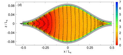
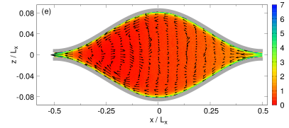
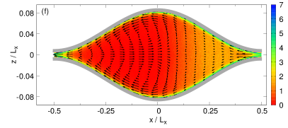
We have then increased the Debye length by reducing the ionic concentration $\rho_{0}$. For $\rho_{0}\sim 1M$ we have $\lambda\simeq 3.1$Å. Hence, the Debye layers of the facing walls overlaps in the narrower sections ($\lambda/h_{\text{min}}\sim 1$, $h_{\text{min}}=6$Å) highlighting that the system is within the entropic electrokinetic regime Malgaretti et al. (2014). Panel b) of Fig. 2 shows that, for $\Delta V=2.4$ [V], the ionic densities are quite affected by the flow. In particular, $Cl^{-}$ concentration largely increases in the channel bottleneck, see e.g. the region $x/L_{x}\in(0.45,0.5)$ in Fig. 2b. This increase in $Cl^{-}$ concentration is associated to $K^{+}$ depletion, that will be discussed more in details in next paragraphs. This feature is associated to the onset of eddies in the electro-osmotic velocity profile, as shown in panels c)-d) of Fig. 2. These eddies form for sufficiently large driving forces. Indeed, while for $\Delta V=0.6$ [V] we do not observe major discrepancies with the previous case, for $\Delta V=2.4$ [V] two eddies form inside the channel. Interestingly, such eddies break down the left-right symmetry of the channel, for instance, Fig. 2d, shows that the eddies are shifted in the direction of the volumetric fluid flow, i.e. negative $x$ in our reference frame. This occurrence is in contrast to the prediction obtained in linear regime Malgaretti et al. (2014) for which the eddies center is in the channel center, $x/L_{x}=0$. Then we further increase the Debye length by setting $\rho_{0}\sim 0.3M$, for which $\lambda\simeq 5.6$Å . In such a regime panels e)-f) of Fig.2 show that the zone in which $K^{+}$ are depleted is enhanced as compared to the previous cases. Moreover, comparing panels e)-f) to c)-d) in Fig.2 we notice that, for $\rho_{0}\sim 0.3M$, the onset of the eddies occurs for smaller values of the external force as compared to $\rho_{0}\sim 1M$.

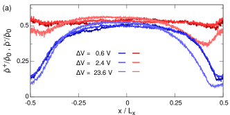
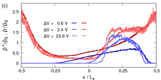
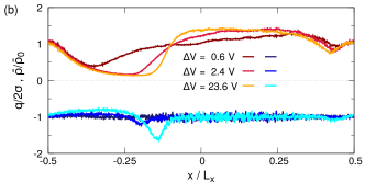
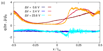
In order to quantitatively capture the accumulation of ions density, we have analyzed the dependence of the ionic densities averaged over the channel section as a function of the longitudinal position. Fig.3 shows that the dependence of normalized densities profiles $\bar{\rho}^{\pm}(x)$ defined as

$$\bar{\rho}_{\pm}(x)\equiv\frac{1}{2h(x)L_{y}}\int\limits_{0}^{L_{y}}dy\int\limits_{-h(x)}^{h(x)}\rho_{\pm}(x,y,z)dz$$ (2)

on the longitudinal position strongly depends on the value of the Debye length as compared to the channel section at the bottleneck. Indeed, when $\lambda/h_{min}\ll 1$, i.e. for $\rho_{0}=3M$, panel a) of Fig.3 shows that the density profiles are almost constant along the channel for all the values of the external force we have tested. The only relevant difference occur close to the narrowest sections $x/L_{x}\simeq\pm 0.5$. In contrast, when $\lambda/h_{min}\sim 1$, i.e. for $\rho_{0}=1M$ and $\rho_{0}=0.3M$ panels b)-c) of Fig.3 show the onset of a region where the coions ($K^{+}$) are depleted and the left-right symmetry is broken. Once we have analyzed the density of $Cl^{-}$ and $K^{+}$ separately we move to the local total charge and local ionic densities defined as:

$$q(x)\equiv 2h(x)\left[\bar{\rho}_{+}(x)-\bar{\rho}_{-}(x)\right]$$ (3)

$$\bar{\rho}(x)\equiv \bar{\rho}_{+}(x)+\bar{\rho}_{-}(x)$$ (4)

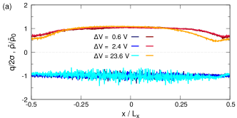
We stress that we choose a different normalization for $q(x)$ and $\bar{\rho}(x)$ so that in a plane channel $|q(x)|$ always match the total surface charge of channel walls $2|\sigma|$ whereas $\bar{\rho}(x)$ is the average density that, in the Debye-Hückel regime, determines the local value of the Debye length. Interestingly, Fig. 4.a shows that in the limit of small Debye lengths, $\lambda/h_{\text{min}}<1$, local electroneutrality is recovered, i.e. $q(x)\simeq 2\sigma$, and the ionic density profile is almost constant along the channel. Only at very high voltages a small deviation is present at $x/L_{x}\simeq 0.4$.

In contrast, for larger values of the Debye length, $\lambda/h_{\text{min}}\simeq 1$, neither $q(x)$ nor $\bar{\rho}(x)$ are constant. Such inhomogeneities trigger the onset of modulations in the magnitude of the local electrostatic potential. In particular, an accurate inspection of panels b)-c) of Fig.4 reveals that weaker values of the external field triggers solely an inhomogeneity in the ionic density but do not affect the local electroneutrality. Interestingly, upon increasing the strength of external electric field local electroneutrality breaks down and on the top of the well-known concentration polarization (CP) Mani and Bazant (2011); Nikonenko et al. (2014); Green et al. (2014); Leese and Mattia (2014); Andersen et al. (2017), a charge polarization (QP) appears.

Figure 4: $\bar{\rho}(x)$ (red curves) and $q(x)$ (blue curves), defined respectively in Eq. (3) and Eq. (4), as a function of the longitudinal position for $\rho=3M$ (panel a), $\rho=1M$ (panel b) and $\rho=0.3M$ (panel c). Lighter color stand for large values of the potential drop $\Delta V$, see legend.

We remark that charge polarization sets for smaller values of the external force for smaller values of the Debye length. This can be due to finite liquid slippage at solid wall that cannot be disregarded in the regime under study. Indeed, slippage is commonly described in term of the Navier boundary condition that, for a plane channel, reads $u_{t}|_{wall}=L_{s}\partial u_{t}/\partial n$ with $u_{t}$ the component of the velocity field tangent to the wall, $n$ the normal to the wall and $L_{s}$ the slip length Lauga et al. (2007). Atomistic simulation showed that for smooth hydrophilic and slightly hydrophobic (contact angle $<120^{\circ}$) surfaces $L_{s}$, hardly exceeds a nanometer Chinappi and Casciola (2010); Huang et al. (2008a); Sega et al. (2013). In addition, the presence of a strong surface charge, further reduces the slip length for hydrophobic surfaces Huang et al. (2008b). When comparing simulations performed with different ionic concentrations it should be taken into account that the slip length $L_{s}$ in the three setups may be slightly different. Indeed, the relevant parameter ruling the effect of slippage on the electroosmotic flow is the ratio $L_{s}/\lambda_{D}$ Bocquet and Charlaix (2010). This feature is emphasized by Fig.S1 in Suppl. Mat. that shows that the mismatch between the prediction of the analytical model (see Ref. Malgaretti et al. (2014)) and the numerical results increases upon decreasing $\lambda_{D}$.

In conclusion, we have reported on numerical simulations concerning a $KCl$ solution embedded in a varying-section channel under the action of a constant electrostatic field. Our simulations show that, when the Debye length is comparable to the width of the channel bottlenecks, the system is in the entropic electrokinetic regime that is characterized by the onset of eddies Malgaretti et al. (2014). In this perspective we observe, in agreement with what has been reported in the literature, the onset of a concentration polarization and local recirculation of the fluid velocity that comes along with the onset of a standing shock in the ionic concentration. Surprisingly, for stronger external fields the local electroneutrality breaks down and an additional charge polarization (QP) sets in. Such a novel phenomena has been observed thanks to our microscopic approach based on Molecular Dynamics simulations in which the ionic densities are not constrained. In this perspective, our results show that for mild external fields local electroneutrality is recovered. This can justify a posteriori the assumption of local electroneutrality in these regimes. However, for larger external fields, local electroneutrality does not hold and a net electric dipole sets in inside the channel.

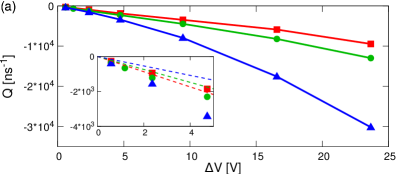
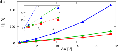
Appendix A Ion and electroosmotic currents

Here, we discuss the dependence of ionic and electroosmotic currents on the applied voltage. Figures 5.a and 5.b show the electro-osmotic flow $Q$ and the ionic current $I$ as a function of the applied electrostatic potential drop $\Delta V=L_{x}E_{x}$ along with the predictions of Poisson-Nernst-Plank (PNP) theory presented in Malgaretti et al. (2014). Both panels of Fig 5 show a significant mismatch between the numerical results (symbols) and the PNP model (dashed lines). Interestingly the mismatch increases upon increasing the salt concentration, i.e. decreasing the Debye length. As discussed in the main text, the effect of the slip on the walls of the channel increases as the ratio $L_{s}/\lambda_{D}$ where $L_{s}$ is the so-called slip length and it captures the magnitude of the slip. In this perspective, Fig.5.a makes us speculate that the mismatch between the numerical results and the PNP model is due to the partial slip of the fluid on the channel walls. Indeed, for high concentration (low $\lambda_{D}$), the MD electro-osmotic flux (blue triangles) is significantly larger than the PNP prediction (dashed blue line). The partial slip can also explain the mismatch shown in Fig.5.b. While in a flat channel an enhancement of the volumetric fluid flow $Q$ leads to an increased electric current (see Ref. Bruus (2008)) the situation is different in the case of a corrugated channel. Indeed, in the latter case the $K^{+}$ ions have to overcome a potential barrier at the channel bottleneck whereas $Cl^{-}$ can move along the channel walls at almost constant potential. Therefore the enhanced $Q$ will reduce the magnitude of the effective barrier that $K^{+}$ have to overcome. Since the flow is quite sensitive to the high of the barrier (for very large barrier the time scales exponentially with the high of the barrier) the enhancement of $Q$ will be more beneficial to the flow of $K^{+}$ as compared to the gain for $Cl^{-}$. Since the electric current is defined as $I=J_{K}-J_{Cl}$ the enhancement of $Q$ leads to a hampered electric current, i.e. the electric currents from MD (symbols) are smaller than the PNP predictions (dashed lines), in particular for larger ionic concentrations.

Figure 5: Electrolyte transport. a): Electro-osmotic flux $Q$ expressed in water molecules per $ns$ as function of $\Delta V$. Different colors stand for different concentrations, namely $\rho_{0}=0.3$M (green circles) $\rho_{0}=1$M (red squares) and $\rho_{0}=3$M (blue triangles). b): Ionic current for different electrostatic potential drops $\Delta V$. Ionic concentrations are color-coded as in panel a). The insets of both panels show the PNP prediction (dashed lines) in the low voltage regime.

Appendix B Methods

System set-up and equilibration. The system is constituted by a KCl water solution confined by two solid walls. The solid walls are formed by atoms arranged in a face centered cubic (fcc) structure with lattice side $a=4.92$ Å. The mass of each atom is $m_{w}=70\;a.m.u.$ and they interact via Lennard-Jones potential with potential well depth $\epsilon_{w}=0.152$ Kcal/mol) and van der Waals radius $\sigma_{w}=3.15$ Å. The curved walls are obtained by solid slabs cut parallel to 111 planes of the fcc solid. The two slabs are then bend to follow the prescribed channel shape with a proper change of the z-coordinate. Each atom exposed to the liquid has a charge $q_{w}$.

Water molecules and ions at a molar concentration $\rho_{0}$ are added using VMD Humphrey et al. (1996). In particular, indicated with $N_{Cl^{-}}$ and $N_{K^{+}}$ the number of Chloride and Potassium ions, we have $N_{Cl^{-}}=1749$ and $N_{K^{+}}=789$ for $\rho_{0}=0.3M$, $N_{Cl^{-}}=3327$ and $N_{K^{+}}=2367$ for $\rho_{0}=1M$, and $N_{Cl^{-}}=8062$ and $N_{K^{+}}=7102$ for $\rho_{0}=3M$. In each case, $N_{Cl^{-}}-N_{K^{+}}=960$. Since $960$e is the total charge on the walls, the total charge of the system is zero.

All MD simulations are performed using NAMD software Phillips et al. (2005) by implementing periodic boundary conditions being $L_{x}=836.6$ Å, $L_{y}=60.37$ Å  and $L_{z}=200$ Å  the box sizes. $L_{x}$ and $L_{y}$ are dictated by the size of solid walls while $L_{z}$ is arbitrary set to $200$ Å  to avoid non-bonded interactions among the different images along the z-axes. The total number of atoms is $\sim$400 000. A snapshot of the system is reported in figure 1.b. Particle mesh Ewalds (PME) summation method was employed for the electrostatics Batcho et al. (2001). TIP3P model Jorgensen et al. (1983) was employed for water while CHARMM36 force field Brooks et al. (2009); Vanommeslaeghe and MacKerell Jr (2012) with NBFIX corrections is used for the ions Luo and Roux (2009). More accurate water models are available, see e.g. the TIP4P_2005 Abascal and Vega (2005) often used for nanofluidics Gentili et al. (2014); Tinti et al. (2017). However, these models are much more computational demanding than TIP3P, hence, in this work, beside the well known limitations of TIP3P (e.g. the viscosity is lower than the experimental value) we preferred TIP3P since it allowed us to run longer simulations and to partially reduce the statistical error.

Walls atoms are constrained at their initial position by harmonic springs (spring constant $k=10$ Kcal/(mol Ų)). A first $0.8$ ns NVT simulations ($T=310$K, time step $2$ fs) was run and pressure is estimated from the average force acting on the walls. The distance between the upper and lower wall is then gradually reduced and further $0.8$ ns simulations are run until the pressure reached a value close to $1$ atm.

Production runs. As common in the MD studies on ionic and electroosmotic transport, a homogeneous and constant external electric field ${\bf E}=(E_{x},0,0)$ is applied to the whole system Aksimentiev and Schulten (2005); Wilson et al. (2016); Bonome et al. (2017). Snapshots are acquired every $\Delta t=2$ps.

The water velocity field in the x,z plane is calculated as follows. The velocity ${\bf v_{i}}$ of the i-th water molecule is estimated as ${\bf v}_{i}=[{\bf x}_{i}(t+\Delta t)-{\bf x_{i}}(t)]/\Delta t$ where ${\bf x_{i}}$ is the position of the oxygen atom of the i-th water molecule. The mean velocity of each particle ${\bf v_{i}}$ is associated to the point ${\bf\hat{x}}_{i}=[{\bf x}_{i}(t+\Delta t)+{\bf x}_{i}(t)]/2$. The value of the velocity field ${\bf u}$ in a given point ${\bf x}$ is hence calculated as the mean of the velocities of the particles in the neighborhood of $\bf x$, i.e. the molecule for which ${\bf\hat{x}_{i}}$ belongs to a region $[x-\Delta x/2,x+\Delta x/2]\cap[z-\Delta z/2,z+\Delta z/2]$. The production runs span in a range of $40-90$ ns with longer simulations used for smaller forcing and lower ionic concentration.

References

- Hille (2001) B. Hille, Ion channels of excitable membranes, Vol. 507 (Sinauer Sunderland, MA, 2001).
- Weatherall and Willmott (2015) E. Weatherall and G. R. Willmott, Analyst 140, 3318 (2015).
- Bayley et al. (2000) H. Bayley, O. Braha, and L.-Q. Gu, Advanced Materials 12, 139 (2000).
- Celaya et al. (2017) G. Celaya, J. Perales-Calvo, A. Muga, F. Moro, and D. Rodriguez-Larrea, ACS nano (2017).
- Bonome et al. (2015) E. L. Bonome, R. Lepore, D. Raimondo, F. Cecconi, A. Tramontano, and M. Chinappi, The Journal of Physical Chemistry B 119, 5815 (2015).
- Asandei et al. (2017) A. Asandei, A. Ciuca, A. Apetrei, I. Schiopu, L. Mereuta, C. H. Seo, Y. Park, and T. Luchian, Scientific Reports 7, 6167 (2017).
- Chinappi and Cecconi (2018) M. Chinappi and F. Cecconi, Journal of Physics: Condensed Matter (2018).
- Asandei et al. (2016) A. Asandei, I. Schiopu, M. Chinappi, C. H. Seo, Y. Park, and T. Luchian, ACS applied materials & interfaces 8, 13166 (2016).
- Boukhet et al. (2016) M. Boukhet, F. Piguet, H. Ouldali, M. Pastoriza-Gallego, J. Pelta, and A. Oukhaled, Nanoscale 8, 18352 (2016).
- Huang et al. (2017) G. Huang, K. Willems, M. Soskine, C. Wloka, and G. Maglia, Nature communications 8, 935 (2017).
- Malgaretti et al. (2015) P. Malgaretti, I. Pagonabarraga, and J. M. Rubi, Macromolecular Symposia 357, 178 (2015).
- Malgaretti et al. (2016) P. Malgaretti, I. Pagonabarraga, and J. M. Rubi, J. Chem. Phys. 144, 034901 (2016).
- Bolet et al. (2018) A. Bolet, G. Linga, and J. Mathiesen, Phys. Rev. E 97, 043114 (2018).
- Guo et al. (2013) W. Guo, Y. Tian, and L. Jiang, Accounts of Chemical Research 46, 2834 (2013).
- Balme et al. (2017) S. Balme, T. Ma, E. Balanzat, and J.-M. Janot, Journal of Membrane Science 544, 18 (2017).
- Experton et al. (2017) J. Experton, X. Wu, and C. R. Martin, Nanomaterials 7, 445 (2017).
- Picallo et al. (2013) C. B. Picallo, S. Gravelle, L. Joly, E. Charlaix, and L. Bocquet, Phys. Rev. Lett. 111, 244501 (2013).
- Laohakunakorn and Keyser (2015) N. Laohakunakorn and U. F. Keyser, Nanotechnology 26, 275202 (2015).
- Bacchin (2018) P. Bacchin, Membranes 8 (2018).
- Kalman et al. (2008) E. Kalman, I. Vlassiouk, and Z. Siwy, Advanced Materials 20, 293 (2008).
- Chen and Das (2017) G. Chen and S. Das, The Journal of Physical Chemistry B 121, 3130 (2017).
- Maduar et al. (2015) S. R. Maduar, A. V. Belyaev, V. Lobaskin, and O. I. Vinogradova, Phys. Rev. Lett. 114, 118301 (2015).
- Rubinstein and Zaltzman (2000) I. Rubinstein and B. Zaltzman, Phys. Rev. E 62, 2238 (2000).
- Park et al. (2006) S. Y. Park, C. J. Russo, D. Branton, and H. A. Stone, Journal of Colloid and Interface Science 297, 832 (2006).
- Mani et al. (2009) A. Mani, T. A. Zangle, and J. G. Santiago, Langmuir 25, 3898 (2009).
- Mani and Bazant (2011) A. Mani and M. Bazant, Phys. Rev. E 84, 061504 (2011).
- Green et al. (2014) Y. Green, S. Shloush, and G. Yossifon, Phys. Rev. E 89, 043015 (2014).
- Zangle et al. (2009) T. A. Zangle, A. Mani, and J. G. Santiago, Langmuir 25, 3909 (2009).
- Chang et al. (2012) H.-C. Chang, G. Yossifon, and E. A. Demekhin, Annual Review of Fluid Mechanics 44, 401 (2012).
- Nikonenko et al. (2014) V. V. Nikonenko, A. V. Kovalenko, M. K. Urtenov, N. D. Pismenskaya, J. Han, P. Sistat, and G. Pourcelly, Desalination 342, 85 (2014), special Issue: Electromembrane Processes for Desalination.
- Malgaretti et al. (2014) P. Malgaretti, I. Pagonabarraga, and J. M. Rubi, Phys. Rev. Lett 113, 128301 (2014).
- Leese and Mattia (2014) H. Leese and D. Mattia, Microfluid Nanofluid 16, 711 (2014).
- Jubin et al. (2018) L. Jubin, A. Poggioli, A. Siria, and L. Bocquet, Proceedings of the National Academy of Sciences 115, 4063 (2018).
- Andersen et al. (2017) M. Andersen, K. Wang, J. Schiffbauer, and A. Mani, electrophoresis 38, 702 (2017).
- Lauga et al. (2007) E. Lauga, M. Brenner, and H. Stone, in Springer handbook of experimental fluid mechanics (Springer, 2007) pp. 1219–1240.
- Chinappi and Casciola (2010) M. Chinappi and C. Casciola, Physics of Fluids 22, 042003 (2010).
- Huang et al. (2008a) D. M. Huang, C. Sendner, D. Horinek, R. R. Netz, and L. Bocquet, Physical review letters 101, 226101 (2008a).
- Sega et al. (2013) M. Sega, M. Sbragaglia, L. Biferale, and S. Succi, Soft Matter 9, 8526 (2013).
- Huang et al. (2008b) D. M. Huang, C. Cottin-Bizonne, C. Ybert, and L. Bocquet, Langmuir 24, 1442 (2008b).
- Bocquet and Charlaix (2010) L. Bocquet and E. Charlaix, Chemical Society Reviews 39, 1073 (2010).
- Bruus (2008) H. Bruus, Theoretical microfluidics, Vol. 18 (Oxford university press Oxford, 2008).
- Humphrey et al. (1996) W. Humphrey, A. Dalke, and K. Schulten, 14, 33 (1996).
- Phillips et al. (2005) J. C. Phillips, R. Braun, W. Wang, J. Gumbart, E. Tajkhorshid, E. Villa, C. Chipot, R. D. Skeel, L. Kale, and K. Schulten, 26, 1781 (2005).
- Batcho et al. (2001) P. F. Batcho, D. A. Case, and T. Schlick, 115, 4003 (2001).
- Jorgensen et al. (1983) W. L. Jorgensen, J. Chandrasekhar, J. D. Madura, R. W. Impey, and M. L. Klein, 79, 926 (1983).
- Brooks et al. (2009) B. R. Brooks, C. L. Brooks, A. D. MacKerell, L. Nilsson, R. J. Petrella, B. Roux, Y. Won, G. Archontis, C. Bartels, S. Boresch, et al., Journal of computational chemistry 30, 1545 (2009).
- Vanommeslaeghe and MacKerell Jr (2012) K. Vanommeslaeghe and A. D. MacKerell Jr, 52, 3144 (2012).
- Luo and Roux (2009) Y. Luo and B. Roux, The Journal of Physical Chemistry Letters 1, 183 (2009).
- Abascal and Vega (2005) J. L. Abascal and C. Vega, The Journal of chemical physics 123, 234505 (2005).
- Gentili et al. (2014) D. Gentili, G. Bolognesi, A. Giacomello, M. Chinappi, and C. Casciola, Microfluidics and nanofluidics 16, 1009 (2014).
- Tinti et al. (2017) A. Tinti, A. Giacomello, Y. Grosu, and C. M. Casciola, Proceedings of the National Academy of Sciences , 201714796 (2017).
- Aksimentiev and Schulten (2005) A. Aksimentiev and K. Schulten, 88, 3745 (2005).
- Wilson et al. (2016) J. Wilson, L. Sloman, Z. He, and A. Aksimentiev, Advanced functional materials 26, 4830 (2016).
- Bonome et al. (2017) E. L. Bonome, F. Cecconi, and M. Chinappi, Microfluidics and Nanofluidics 21, 96 (2017).