Abstract

Canonical semiclassical methods can be used to develop an intuitive definition of tunneling time through potential barriers. An application to atomic ionization is given here, considering both static and time-dependent electric fields. The results allow one to analyze different theoretical constructions proposed recently to evaluate ionization experiments based on attoclocks. They also suggest new proposals of determining tunneling times, for instance through the behavior of fluctuations.

1 Introduction

Detailed observations of atom ionization have recently become possible with attoclock experiments [1, 2, 3], suggesting comparisons with various predictions of tunneling times. The theoretical side of the question, however, remains largely open: Different proposals of how to define tunneling times have been made through almost nine decades, yielding widely diverging predictions and physical interpretations [4, 5]. Even the extraction of tunneling times from experiments has been performed in different ways [6, 7, 8, 9, 10, 11], and the original conclusion of a non-zero result has been challenged [12, 13, 14]. The situation therefore remains far from being clarified, and a continuing analysis of fundamental aspects of tunneling is important.

A recent approach to understand the tunneling dynamics in this context is the application of Bohmian quantum mechanics [15, 16], in which the prominent role played by trajectories provides a more direct handle on tunneling times [17]. However, through initial conditions, the ensemble of trajectories remains subject to statistical fluctuations. An alternative trajectory approach, which we will develop in this paper, is to consider, in an extension of Ehrenfest’s theorem, the evolution of expectation values and fluctuations, possibly together with higher-order moments of a state. By including moments of a probability distribution, such an approach remains statistical in order to capture quantum properties, but it provides a unique trajectory starting with the expectation values and fluctuations of a given initial state. The ensemble of trajectories used in Bohmian quantum mechanics is replaced by a single trajectory in an extended phase space, enlarged by fluctuations and higher moments as non-classical dimensions.

In the context of tunneling, a semiclassical version of this proposal has been used occasionally in quantum chemistry [18, 19], which we extend here to higher orders and apply to models of atom ionization. Unlike Bohmian quantum mechanics, these methods present an approximation to standard quantum mechanics, rather than a new formulation. Nevertheless, since they lead to a single trajectory rather than a statistical ensemble of trajectories, they provide a crucial advantage which, we hope, can help to clarify the question of tunneling times in atom ionization.

In [17], it has been shown that a trajectory approach based on Bohmian quantum mechanics reliably shows non-zero tunneling times in atomic models of ionization. There is therefore a tension with recent evaluations of ionization experiments which give the impression of zero tunneling delays [13]. The latter results are based on a definition of the tunneling exit time through classical back-propagation [12]: Since the energy of a tunneling electron in a time-dependent electric field is not conserved and usually unkonwn in experiments, it is difficult to apply the intuitive definition of the tunneling exit as the time when the electron’s energy equals the classical potential. As an alternative, classical back-propagation evolves the final state of a measured electron back toward the atom using classical equations of motion, and defines the tunneling exit as the time when the momentum in the direction of the electric field is zero, taking the point closest to the atom in the event that this condition may be realized multiple times. As already noted in [17], this condition is conceptually problematic because it uses classical physics near a turning point, where the equations governing a classically back-propagated trajectory are usually expected to break down. We will use our single-trajectory approach to compare a quantum trajectory with a classical back-propagated one.

In addition, our analysis will allow us to derive further properties of the tunneling process. In order to obtain a single trajectory describing an evolving quantum state, we write evolution of a quantum state in terms of a classical-type system with quantum corrections, in which the expectation values of position and momentum are coupled to fluctuations. The coupling terms, quite generally, lower the classical barrier such that the classical-type system can move “around” it in an extended phase space with a real-valued velocity. This detour has a certain duration, depending on initial conditions, and provides a natural definition of tunneling time.

It turns out that several new ingredients are necessary compared with existing treatments in quantum chemistry. For instance, semiclassical states are not always sufficient for a full description of tunneling. This fact is not surprising because, intuitively, a tunneling wave splits up into two wave packets separated by the barrier width. Deep tunneling then implies states with large fluctuations, even if each wave packet remains sharp and perhaps nearly Gaussian. Moreover, fluctuation terms do not always lower the barrier enough to make tunneling possible at all energies for which quantum tunneling occurs. In [19], the classical-type system used for tunneling has been extended to moments of up to fourth order, with a clear improvement of predicted tunneling times closer to what follows from wave-function evolution. However, the extension was done mainly at a numerical level, which does not provide much intuition about the tunneling process in a given potential. To second order, by contrast, an effective potential was used in [18, 19] which shows how the classical barrier can be lowered by quantum fluctuations. One of our main new ingredients is an extension of such effective potentials to higher orders.

In Sec. 2 we describe quantum dynamics using canonical semiclassical methods and present a new effective potential that includes effects from higher-order moments. In Sec. 3, we introduce various models of atom ionization in which our methods can be applied, and discuss specific results focusing on tests of tunneling conditions and the definition of tunneling times.

2 Quantum dynamics by canonical effective methods

Using canonical effective methods [20, 21], we describe the dynamics of a quantum state by coupled ordinary differential equations for the expectation values $x=\langle\hat{x}\rangle$ and $p=\langle\hat{p}\rangle$ coupled to central, Weyl-ordered moments

$$\Delta(x^{a}p^{b})=\langle(\hat{x}-x)^{a}(\hat{p}-p)^{b}\rangle_{\rm Weyl}\,.$$ (1)

(In this notation, the usual fluctuations are written as $\Delta(x^{2})=(\Delta x)^{2}$ and $\Delta(p^{2})=(\Delta p)^{2}$, while $\Delta(xp)$ is the covariance.)

The Hamiltonian operator $H(\hat{x},\hat{p})$ implies the quantum Hamiltonian

$$H_{{\rm Q}} = \langle H(\hat{x}+(\hat{x}-x),\hat{p}+(\hat{p}-p))\rangle$$ (4)

$$= H(x,p)+\sum_{n=2}^{\infty}\sum_{a=0}^{n}\left(\begin{array}[]{c}n\\ a\end{array}\right)\frac{\partial^{n}H(x,p)}{\partial x^{a}\partial p^{n-a}}\Delta(x^{a}p^{n-a})$$

with the classical Hamiltonian $H(x,p)$. Hamiltonian equations for moments are generated using the Poisson bracket

$$\{\langle\hat{A}\rangle,\langle\hat{B}\rangle\}=\frac{\langle[\hat{A},\hat{B}]\rangle}{i\hbar}\,,$$ (5)

derived from the commutator and extended to moments by using linearity and the Leibniz rule.

Unfortunately, the Poisson brackets between moments are rather complicated at higher orders, and they are not canonical. For instance,

$$\{\Delta(x^{2}),\Delta(xp)\}=2\Delta(x^{2})\quad,\quad\{\Delta(x^{2}),\Delta(p^{2})\}=4\Delta(xp)\quad,\quad\{\Delta(xp),\Delta(p^{2})\}=2\Delta(p^{2})\,,$$ (6)

corresponding to the Lie algebra ${\rm sp}(2,{\mathbb{R}})$, but those of higher moments are in general non-linear. For these second-order moments, canonical variables were introduced in [18, 19]:

$$s=\sqrt{\Delta(x^{2})}\quad,\quad p_{s}=\frac{\Delta(xp)}{\sqrt{\Delta(x^{2})}}$$ (7)

together with a third variable, $U=\Delta(x^{2})\Delta(p^{2})-\Delta(xp)^{2}$, which has zero Poisson brackets with $s$ and $p_{s}$. Inverting these relationships, we write the second-order moments

$$\Delta(x^{2})=s^{2}\quad,\quad\Delta(xp)=sp_{s}\quad,\quad\Delta(p^{2})=p_{s}^{2}+\frac{U}{s^{2}}$$ (8)

in terms of canonical variables $(s,p_{s})$ and a conserved quantity $U$. To second order, the quantum Hamiltonian can then be expressed as

$$\langle\hat{H}\rangle = \frac{\langle\hat{p}^{2}\rangle}{2m}+\langle V(\hat{x})\rangle$$ (9)

$$\approx \frac{\langle\hat{p}\rangle^{2}}{2m}+\frac{(\Delta p)^{2}}{2m}+V(\langle\hat{x}\rangle)+\frac{1}{2}V^{\prime\prime}(\langle\hat{x}\rangle)(\Delta x)^{2}=\frac{p^{2}+p_{s}^{2}}{2m}+V_{\rm eff}(x,s)$$

with the effective potential

$$V_{\rm eff}(x,s)=V(x)+\frac{U}{2ms^{2}}+\frac{1}{2}V^{\prime\prime}(x)s^{2}\,.$$ (10)

An extension to higher orders turns out to be more involved, but it can be accomplished with the new methods developed in [22]. The canonical form of higher-order moments then gives useful higher-order effective potentials, and it suggests closure conditions, in the sense of [23], that can be used to turn the infinite set of moments into finite approximations.

We introduce closure conditions based on the following properties of higher moments which we have confirmed for up to fourth order [24]: the second-order variable $s$ also contributes to an $n$-th order moment, in the form $\langle(\hat{x}-\langle\hat{x}\rangle)^{n}\rangle\approx s^{n}$, in addition to terms that depend on new degrees of freedom. Moments of odd and even order, respectively, often behave rather differently from each other. For instance, a Gaussian has zero odd-order moments, a property which extends to generic states that evolve adiabatically in symmetric potentials [20]. This difference is reflected in mathematical properties of the canonical variables. At third order, for instance, there are three canonical coordinates, $s_{1}$, $s_{2}$ and $s_{3}$, such that $\langle(\hat{x}-\langle\hat{x}\rangle)^{3}\rangle\propto s_{1}^{3}+s_{2}^{3}+s_{3}^{3}$. The constant of proportionality has zero Poisson brackets with the canonical variables but is state dependent. As an approximation, we set this constant equal to zero, reducing the number of degrees of freedom. If we assume this behavior also for orders greater than four, we can complete the Taylor expansion in (4) and derive the all-orders effective potential

$$V_{\rm eff}(x,s) = \frac{U}{2ms^{2}}+V(x)+\sum_{n=1}^{\infty}\frac{1}{2n!}\frac{{\rm d}^{2n}(V(x))}{{\rm d}x^{2n}}s^{2n}$$ (11)

$$= \frac{U}{2ms^{2}}+\frac{1}{2}\left(V(x+s)+V(x-s)\right)\,.$$

Heuristically, therefore, the particle does not follow a potential local in $x$, but rather is feeling around itself at a distance $s$. This distance increases as the wave function spreads out.

We have moved beyond the semi-classical approximation by replacing a strict truncation with a specific behavior of the moments. This extension is crucial for our purposes because tunneling states or the ground states of an electron in most atoms are not semi-classical. A semi-classical approximation should then not be expected to give accurate results in situations where the tunneling times are very long, or the electron spends a fair amount of time in states close to the ground state.

3 Effective theory of tunneling ionization

In order to test various aspects that have been found to be relevant for tunneling times in ionization experiments, we discuss properties and results of different models. An application to tunneling ionization requires an extension of (11) to three dimensions. The main question is then how to deal with cross-correlations between different coordinates, which significantly enlarge the phase space. Motivated by the intuition that a tunneling wave packet should split up predominantly in the direction of the force that lowers the confining potential of a bound state, we assume that the main moments to be considered are the two fluctuations (position and momentum) in the direction of the force. These moments then play the role of reaction coordinates [25], which reduce a large parameter space to a few significant variables.

The relationship to the direction of the force implies a crucial difference between the treatment of a constant force and time-dependent, rotating forces as used in attoclock experiments. We first deal with examples subject to a constant force in order to illustrate the tunneling process with our new methods, and then show how time-dependent forces alter the conclusions.

3.1 Coulomb potential in a static electromagnetic field

As usual, we can treat tunneling ionization as a a single electron moving in an effective potential with two contributions: a spherically symmetric term for interactions with the nucleus and the remaining electrons, and a linear potential in the direction of the electric field. Assuming that correlations between the independent coordinates can be ignored, an approximation that can be expected to be valid during most of the tunneling process which affects mainly one of the coordinates, the all-orders effective potential (11) for the 3-dimensional Coulomb interaction and the electric field strength $F$ is then

$$V_{\rm eff}(x_{i},s_{j})=\sum\limits_{i=1}^{3}\frac{U}{2s_{i}^{2}}+\frac{1}{8}\sum\limits_{\{n_{i}=0,1\}}V\left(x_{i}+(-1)^{n_{i}}s_{i}\right)\,,$$ (12)

where

$$V(\vec{x})=-\frac{1}{|\vec{x}|}-\vec{x}\cdot\vec{F}-\frac{\alpha_{I}\vec{F}\cdot\vec{x}}{|\vec{x}|^{3}}$$ (13)

is the classical potential and $\alpha_{I}$ is the static polarizability of the ion. (We set $\vec{x}=(x,y,z)$ and use atomic units $\hbar=e=m_{e}=k_{e}=1$ throughout the paper.)

Evolution in the effective potential requires initial values of $x_{i}$, $s_{i}$, $p_{i}$ and $p_{s_{i}}$. Since these describe expectation values and fluctuations, they could in principle be determined from an initial atomic state. However, it is more useful to minimize the energy in the field-free ($\vec{F}=0$) effective potential (12), in order to fix these initial values within our approximation. That is, to get initial values for the canonical variables we minimize $\frac{1}{2}\sum(p_{i}^{2}+p_{s_{i}}^{2})+V_{\rm eff}(\vec{x},\vec{s})$ in the absence of the electric field. We find

$$s_{i}^{0}=\frac{3\sqrt{3}}{4}\quad\mathrm{and}\quad p_{i}^{0}=p_{s_{i}}^{0}=x_{i}^{0}=0$$ (14)

for $i=1,2,3$. These values, taken as initial conditions for tunneling with a non-zero field, result in a ionization potential of $I_{p}=-2/9$ which in our model corresponds the ground-state energy $E_{\rm ground}$ in the absence of the electric field.

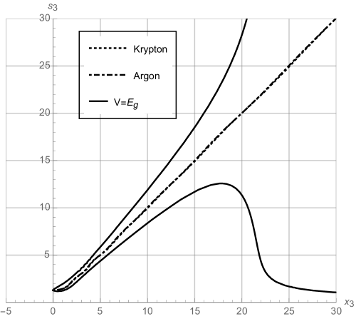
Figure 1: A contour plot of the effective potential for both Argon ($\alpha_{I}=7$) and Krypton ($\alpha_{I}=11$). The solid curve is the equipotential line, $V_{\rm eff}=E_{\rm ground}=-2/9$ for the approximate ground-state energy corresponding to (14). It shows the location of the classical barrier in the presence of a field $F=0.015$ (a laser intensity of $I\sim 0.8\cdot 10^{14}{\rm W}/{\rm cm}^{2}$). The path of the electron is shown here by the (almost overlapping) dashed lines for Argon and Krypton. The electron escaping from either atom has to travel along an actual tunnel, formed by the equi-potential line in phase space.

We choose our coordinate system such that the $x_{3}$-axis points in the direction of the force. Figure 1 shows the ground-state equipotential line of (12) in the $x_{3}-s_{3}$ plane for both Argon ($\alpha_{I}=7$) and Krypton ($\alpha_{I}=11$), as well as the behavior of the fluctuation parameter $s_{3}$ with respect to the direction along $x_{3}$. When the field strength is small enough, the equipotential line of the ground state literally forms a tunnel that the electron has to follow in order to escape. The tunneling time is related to the amount of time spent in this tunnel. At this point, we can see the importance of our extension beyond semiclassical effective potentials. The quadratic $s$-term in (10) reduces the classical barrier monotonically in the $s$-direction, giving us a steep slope instead of a tunnel. Numerical solutions in such a potential show that the resulting tunneling times would be too large because trajectories get dragged into the $s$-direction with little movement in the $x$-direction. The tunnel in our all-orders potential, by contrast, guides the trajectories such that they still move substantially in the $x_{3}$-direction. Corresponding tunneling times are significantly shorter.

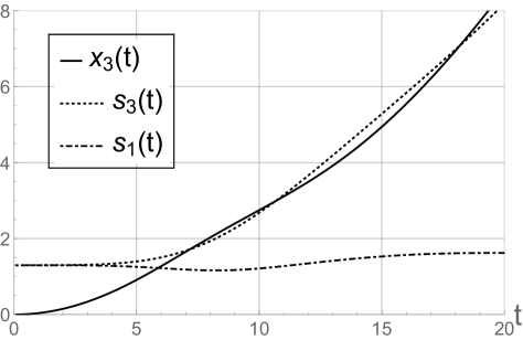
Figure 2: Trajectories of the tunneling coordinate $x_{3}$, its fluctuation $s_{3}$ and the fluctuation $s_{1}$ for Argon. The behavior for Krypton is qualitatively similar.

Our dynamical system contains not only expectation values but also the fluctuation variables $s_{i}$ and $p_{s_{i}}$, related to $\Delta x_{i}$ and $\Delta p_{i}$ as in (8). As shown in Fig. 2, our effective evolution is self-consistent in the sense that it is indeed only the fluctuation $s_{3}$ in the direction of the force (our reaction coordinate) that increases significantly, while $s_{1}$ and $s_{2}$ remain nearly constant. Nevertheless, the behavior of the transversal position fluctations, shown in Fig. 3 for the example of $s_{1}$ at the tunneling exit, is also of interest: There is a local minimum with a value less than the ground-state fluctuation (14). At higher intensities, the fluctuations level off because in a strong field they do not have much time to change. Moreover, these fluctuations depend more strongly on the element used compared to the trajectories in Fig. 1 for variables in the direction of the force, or the tunneling time to which we turn now.

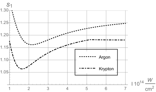
Figure 3: The transverse exit fluctuation $s_{1}$ over the observable range of laser intensities for Argon and Krypton.

Using the all-orders potential in a static field, we estimate the tunneling time in Argon and Krypton as a function of the laser intensity. The tunneling time is determined by how long the particle travels from one turning point to another in a state parameterized by $x_{i}$ and $s_{i}$. The tunneling times for both Argon and Krypton in the range of laser intensities used in [2], are shown in Fig. 4. We see tunneling at all relevant scales, and qualitative agreement with the calculations from Wigner formalism used in [2].

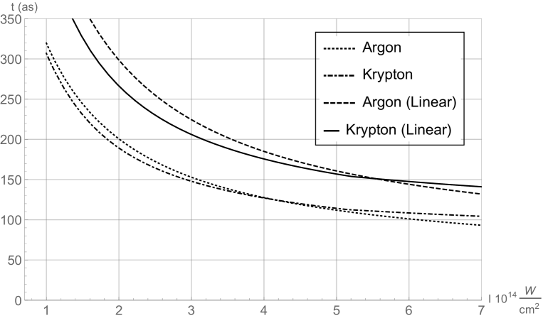
Figure 4: Tunneling times for Argon and Krypton. The dashed (Argon) and solid (Krypton) lines correspond to the approximation (15) with $s_{3}\approx x_{3}$. The range of the laser intensity is obtained by scaling the electric field $I=\frac{1}{2}c\epsilon_{0}F^{2}$. Time variables are scaled to atto-seconds from atomic units.

Traditionally, proposed tunneling times have often been expressed as integral formulas, motivated by the WKB approximation. Our effective potential can be used to derive a new version if we eliminate some of the basic variables in further approximations. As suggested by Figs. 1 and 2, we may assume that $s_{3}\approx x_{3}$ inside the barrier. The tunneling time can then be written as

$$\tau\approx\int^{x_{3}^{*}}_{0}\frac{{\rm d}x_{3}}{p_{3}}\approx\int^{x_{3}^{*}}_{0}\frac{{\rm d}x_{3}}{\sqrt{-E_{\rm ground}-V_{\rm{eff}}(x_{i},\tilde{s}_{i})}}\,,$$ (15)

where $\tilde{s}_{3}=x_{3}$ and $x_{3}^{*}$ is the tunneling exit position. The values of $x_{1}$ and $x_{2}$ are assumed zero, while $\tilde{s}_{1}$ and $\tilde{s}_{2}$ retain their ground-state values. The qualitative behavior of the tunneling time in Fig. 4 under this approximation is not too far from the results of our full computation.

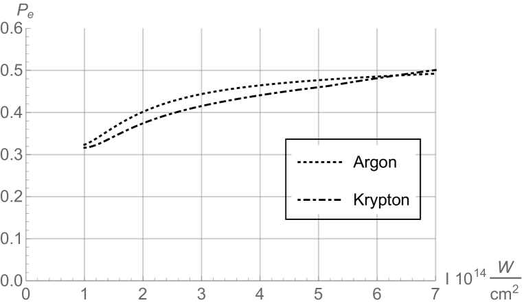
Figure 5: Exit momenta for the electron as a function of the laser intensity. They have the same qualitative behavior as in [2] with an agreement of order of magnitude.

Our method also yields the momentum $p_{3}$ at the tunnel exit, shown in Fig. 5. The longitudinal momentum is non-zero because the electron exits the tunnel with momentum in the direction of the force: As shown in Fig. 1, in the effective potential, the classical turning point is replaced by an actual tunnel exit. Our effective potential therefore presents a self-contained model in which several observational features are qualitatively reproduced, without any free parameters beyond the coefficients used to define the classical potential. However, it requires an extension to time-dependent forces modelling laser fields.

3.2 Time-dependent, circularly polarized electric fields

If the direction of the force is not constant, tunneling should affect the moments of more than one degree of freedom. If the force is rotating at constant angular velocity $\omega$, we can nevertheless find suitable reaction coordinates by transforming to a frame co-rotating with the force. It is sufficient to start with a two-dimensional system in the plane in which the force is rotating. For instance, the example used in [13] is a two-dimensional, time-dependent vector potential

$$\vec{A}(t)=\frac{A_{0}}{\sqrt{1+\epsilon^{2}}}\cos^{4}(\omega t/2N)\left(\begin{array}[]{c}\cos(\omega t)\\ \epsilon\sin(\omega t)\end{array}\right)$$ (16)

for $N$ cycles of frequency $\omega$, with ellipticity $\epsilon$. The corresponding electric field is

$$\vec{E}=-\frac{{\rm d}\vec{A}}{{\rm d}t}=\frac{A_{0}\omega}{\sqrt{1+\epsilon^{2}}}\cos^{4}(\omega t/2N)\left(\begin{array}[]{c}\sin(\omega t)+\frac{2}{N}\tan(\omega t/2N)\cos(\omega t)\\ \epsilon\left(-\cos(\omega t)+\frac{2}{N}\tan(\omega t/2N)\sin(\omega t)\right)\end{array}\right)\,.$$ (17)

Specialized to two cycles, $N=2$, and circular polarization, $\epsilon=1$, also as in [13], we have

$$\vec{E}=\frac{A_{0}\omega}{\sqrt{2}}\cos^{3}(\omega t/4)\left(\begin{array}[]{c}\sin(5\omega t/4)\\ \cos(5\omega t/4)\end{array}\right)=\frac{A_{0}\omega}{\sqrt{2}}\cos^{3}(\omega t/4)S\left(\begin{array}[]{c}1\\ 0\end{array}\right)$$ (18)

with the orthogonal matrix

$$S=\left(\begin{array}[]{cc}\sin(5\omega t/4)&-\cos(5\omega t/4)\\ \cos(5\omega t/4)&\sin(5\omega t/4)\end{array}\right)\,.$$ (19)

In terms of the electric field, we can write the Hamiltonian for a negatively charged particle as

$$H=\frac{1}{2}\vec{p}^{2}+\vec{r}\cdot\vec{E}+V(r)\,.$$ (20)

In co-rotating coordinates

$$\vec{R}=S^{-1}\vec{r}\quad,\quad\vec{P}=S^{-1}\vec{p}$$ (21)

we have

$$H=\frac{1}{2}\vec{P}^{2}+\vec{R}\cdot\vec{E}_{0}+V(R)+\frac{5\omega}{4}\left(P_{1}R_{2}-P_{2}R_{1}\right)$$ (22)

with an electric field

$$\vec{E}_{0}=S^{-1}\vec{F}=\frac{A_{0}\omega}{\sqrt{2}}\cos^{3}(\omega t/4)\left(\begin{array}[]{c}1\\ 0\end{array}\right)\,,$$ (23)

which is not constant but points in a fixed direction. The fluctuations in this direction are our reaction coordinates.

The transformation to a co-rotating frame shows that the two-dimensional nature of tunneling in circularly polarized electric fields is not essential, but it turns out that the non-static behavior of the field amplitude is important. This behavior can be studied by Bohmian quantum mechanics in one-dimensional models [17], or by our effective potentials as we will do in the rest of this paper.

For our methods, in the one dimensional case, it is of advantage to have a smooth potential which is finite everywhere. Instead of the Coulomb potential or the truncated version of [17], we therefore consider a one-dimensional model for a Gaussian potential well in a time-dependent electric field:

$$V(x,t)=-\,\frac{e^{-x^{2}}}{2}+x\,F(t)\,.$$ (24)

The potential depth is chosen so that the ground state energy agrees with $E_{\rm ground}$. As the time-dependent electric field, we choose, as in [17],

$$F(t)=\left\{\begin{array}[]{cl}-F_{0}\sin(\omega t)^{2}\sin(\omega t)&\mbox{if }0<t<\frac{\pi}{\omega}\\ 0&\mbox{otherwise,}\end{array}\right.$$ (25)

which has an amplitude of $F_{0}$, frequency $\omega=0.05811$, and starts at time $t=0$. Compared with [13], this field belongs to a half-cycle pulse, $N=1/2$. The corresponding intensities are considered in the observed regime. We will use the form (25) in our examples, and later on comment on some of the differences compared with (23).

We use this model in order to probe different definitions of the time when the electron exits the tunnel. The standard definition of tunneling exit points equates the energy of the particle with the potential, at which time a classical turning point would be reached in the absence of quantum corrections. As shown in [12, 13, 14], this condition cannot always be imposed in non-static situations, in which the energy of the electron is not constant and may not be known in an experiment. As an alternative, these papers proposed classical back-propagation as a new method, combined with a definition of the tunneling exit as the time when the momentum of the particle in the direction of the force, evaluated on a classically back-propagated trajectory, is zero. However, while this condition is of advantage in evaluations of experimental results [13, 14], it is questionable, as also pointed out in [17], because it makes use of a classical property (zero longitudinal momentum at a classical turning point) in a region where classical physics is known to be inadequate. Our methods describe tunneling by a single quantum trajectory, which we will compare directly with the back-propagated classical trajectory in order to see possible deviations.

3.3 Definition of tunneling time for dynamic fields

The main quantity of conceptual interest is called “tunneling traversal time” in [17], which is the time the electron spends in a classically forbidden region between two turning points. In a constant field, the positions of turning points depend only on the initial energy of the electron and can be easily determined, but the definition is more difficult to implement when the dynamical behavior of the force is crucial [13].

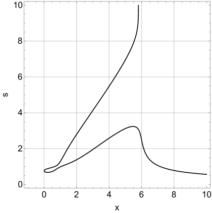
Figure 6: Equipotential plot of the all orders at potental at $t=16$, about half-way to the wave peak.

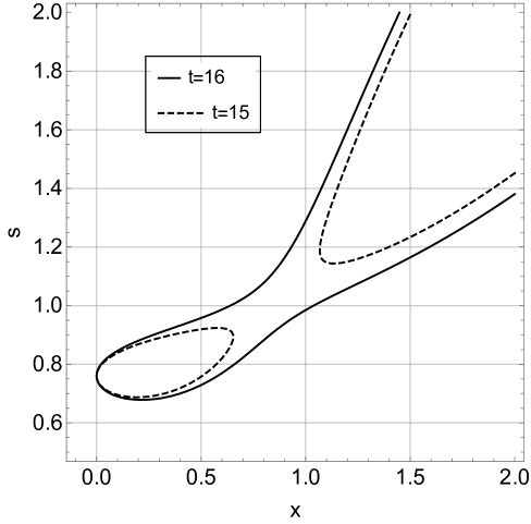
Figure 7: Zoom-in of Fig. 6 on the area of interest. The dashed contour is from $t=15$ at which time the tunneling channel has not completely opened. A little while later, at $t=16$, the tunneling channel is open and the particle can leave.

As a solution, [13] proposed the method of classical back-propagation in order to determine the “tunneling exit time” defined as the point in time when the electron reenters a classically allowed region. By definition, the tunneling exit time is therefore a point in time, while the tunneling traversal time is a duration. The examples considered in [13] suggested near-zero tunneling exit times, which has to be interpreted in the context of the pulse (23) with maximum intensity at time zero. In the terminology of [17], the tunneling exit time of [13] is therefore equal to the “tunneling ionization time” defined as the duration between the maximum of the external force and the time when the electron reenters a classically allowed region.

The tunneling ionization time can be accessed in observations more directly than the tunneling traversal time. But it does not give us a full picture of the tunneling process because the electron may well start tunneling before the external force has reached its maximum. The near-zero tunneling exit times or tunneling ionization times of [13] therefore do not imply that the electron tunnels without any delay. The example of tunneling times given in [17] illustrates this difference, which we can show explicitly using our effective potential: As shown in Figs. 6 and 7, the tunnel has already opened as early as halfway through the build-up of the external force.

In the next subsection, we will analyze tunneling exit criteria, and then return to the question of tunneling traversal.

3.4 Tunneling exit criteria for dynamic fields

For the time-dependent potential (24) we should use a definition of tunneling exit time which can account for non-adiabatic effects. For instance, the energy condition

$$H_{\rm Q}(p(t),p_{s}(t),x(t),s(t);t)-x(t)\,F(t)=0$$ (26)

gives us a finite time because we always have $V_{\rm eff}<0$ when the term $U/2ms^{2}$ can be ignored. This definition focuses on the energy gain in an external force: By the time the electron reaches zero energy, it is in an allowed region for any negative potential. In this condition, quantum effects can be significant, for instance when the kinetic energy $p_{s}^{2}/2m$ of fluctuations raises the energy to positive values; see Fig. 9 below. The condition is adapted to non-adiabatic situations, in the sense that the dynamically changing energy is kept track of. While this criterion includes non-adiabatic effects, the quantum dynamics is approximated by an all orders Hamiltonian. The canonical tunneling exit time is taken to be the instant when (26) is satisfied.

We present results from numerical simulations with the quantum Hamiltonian (9) for an effective potential (12) and the initial conditions (14). We mainly show the tunneling exit time $\tau_{\rm ex}$ by extracting the instant when the interaction-free part of the quantum Hamiltonian (26) crosses the time axis. From this value, we are able to determine the tunneling ionization time $\tau_{\rm ion}=\tau_{\rm ex}-\tau_{\rm max}$, which is defined with respect to the instant of maximum field, $t=\pi/2\omega$ in (25); see Fig. 8. In particular, the tunneling ionization time $\tau_{\rm ion}$ is several atomic units for a field amplitude $F_{0}=0.14$ and becomes smaller for higher intensity pulses. Figure 9 shows that the “quantum” kinetic energy $T_{Q}=p_{s}^{2}/2m$ is important for an evaluation of this condition. The tunneling exit time of the electron in Fig. 8 explicitly indicates non-zero tunneling ionization time for a dynamic barrier, similarly to what has been obtained in [2, 6, 7] but on a smaller scale.

Figure 8: The tunneling exit time as an energy condition: $H_{\rm Q}-x\,F=0$. The intermittent lines represent this condition with respect to time parameter $t$ for three different electric field amplitudes (corresponding to an intensity range of $F_{0}^{2}\sim[6\times 10^{14},12\times 10^{14}]\,{\rm W/cm^{2}}$). The vertical solid line indicates the instant of maximum field strength at $\tau_{\mathrm{max}}\sim 27$ atomic units.

Figure 9: The energy as a function of time, with the kinetic term of the quantum degrees of freedom removed.

In addition, laser pulses of sufficiently high frequency do not lead to tunneling if we keep the same maximal field amplitude for varying frequencies; see Fig. 10. This implication is easy to understand because less energy then falls on the atom. However, if we use pulses with various frequencies and intensities such that there is always the same energy hitting the atom, we find that, as the frequency rises, the tunneling exit criterion gives ionization times that tend to zero. In this limit, most of the energy reaches the atom close to the wave peak. The result is conceptually similar to the traditional distinction between tunneling ionization and multiphoton ionization based on the Keldysh parameter $\gamma_{\rm K}=\omega\tau_{\rm K}$ with $\tau_{\rm K}=\sqrt{2|I_{p}|}/F$ [26, 27]. If $\gamma_{\rm K}\gg 1$, the pulse frequency $\omega$ is too large to allow a process of duration $\tau_{\rm K}$ to be completed during a laser cycle, which suggests that tunneling does not take place at high frequency. However, the Keldysh time $\tau_{\rm K}$ refers to the ionization potential $I_{p}$ and is therefore adapted to a static electric field during tunneling.

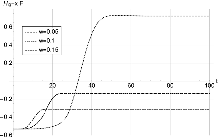
Figure 10: Above a certain critical frequency we no longer obtain tunneling according to the condition (26).

Our method of approximating quantum dynamics allows us to compare different possible tunneling criteria, in particular criteria based on momentum and energy conditions for the tunnel exit. The recent study [13], analyzing a model for a single active electron in a helium atom, obtains a near-zero ionization time using classical backpropagation and zero longitudinal momentum to define the tunneling exit time. The basic idea of classical backpropagation is to evolve the initial state quantum-mechanically forward to some time after the laser pulse has ended. Then, the classically transmitted ionized part of the wave packet is backpropagated and tunneling exit properties are extracted corresponding to the specific tunneling criterion applied.

Figure 11: Quantum trajectory (solid line) going forwards and the classical trajectory (dashed line) being back propagated in time. The quantum Hamiltonian is responsible for the evolution of the quantum trajectory. The back propagated trajectory is obtained by first evolving the classical trajectory backward in time with the initial condition of the quantum trajectory at some later time.

We can compare the momentum condition with the energy condition that we introduced in (26). First, we evolve the system by the quantum Hamiltonian in (9) forward to some late time, $t\sim 150$. Then, using the final values of $\{\langle\hat{x}\rangle,\langle\hat{p}\rangle\}$ at the late time as initial conditions of position and momentum $\{x_{\rm bp},p_{\rm bp}\}$, we use the classical Hamiltonian $H_{\rm cl}\equiv p^{2}/2+V(x)$ to backpropagate classically to an early time. Figure 11 shows that the backpropagation trajectory of the particle stays rather close to the quantum evolved trajectory. However, the backpropagated trajectory deviates from the effective trajectory around the instant ($t\approx 27$) when the electric field amplitude is maximum, close to the tunneling exit, where it bounces off the potential well. In Fig. 12 we show how the tunneling exit time is realized with respect to the momentum condition based on classical backpropagation. There is a non-zero tunneling ionization time $\tau_{\rm ion}\sim 3$ (atomic units) in qualitative agreement with but smaller than what we obtained from the energy condition.

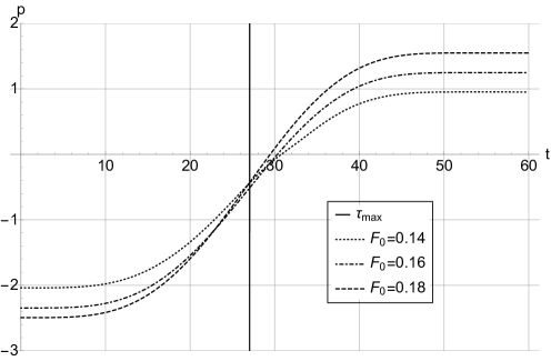
Figure 12: Momentum, as a function of time, being back propagated in time. The intermittent lines represent the momentum condition with respect to time parameter $t$ for the same three different electric field amplitudes used for the energy condition. The vertical line indicates the instant of maximum field strength $\tau_{\mathrm{max}}\sim 27$ atomic units.

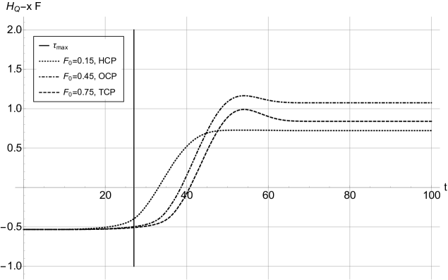
Figure 13: The tunneling energy condition as a function of time for various pulses with different field amplitudes: HCP (half-cylce pulse, $F_{0}=0.15$), OCP (one-cycle pulse, $F_{0}=0.45$), TCP (two-cycle pulse, $F_{0}=0.75$).

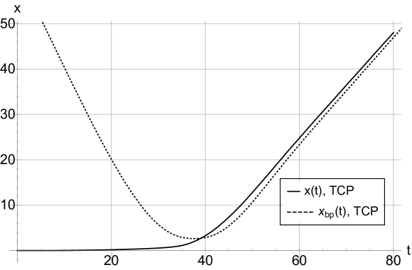
Figure 14: Quantum trajectory (solid line) going forwards and the classical trajectory (dashed line) being back propagated in time for a two-cycle pulse. The quantum Hamiltonian is responsible for the evolution of the quantum trajectory.

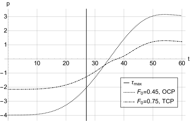
Figure 15: Momentum, as a function of time, being back propagated in time for both one- and two-cycle pulses. The intermittent lines represent the momentum condition with respect to time parameter $t$ for the same three electric field amplitudes used for the energy condition.

So far, our results have been shown for a half-cycle pulse (25), while [13] used a two-cycle pulse. We repeated our calculations for one- and two-cycle pulses while keeping the same frequency used in the half-cycle pulse, see Fig. 13. Figures 14 and 15 confirm our general findings, and they show that tunneling is possible for significantly larger field amplitudes than for a half-cycle pulse (for which less energy falls on the atom). The frequency dependence of tunneling times can also be confirmed. More cycles in a pulse of the same frequency produce a longer tunneling ionization time according to both criteria evaluated here because the field intensity rises more slowly for bigger $N$.

3.5 Tunneling dynamics of Hydrogen in three dimensions

As the most realistic one of our models, we now consider the three dimensional case of a Hydrogen atom in a time dependent electric field

$$H=\frac{1}{2}|\vec{p}|^{2}-\frac{1}{|\vec{r}|}+\vec{r}\cdot\vec{E}(t)\,,$$ (27)

where we use a half cycle pulse

$$\vec{E}(t)=-E_{0}\sin^{2}{(\omega t)}\theta(t)\theta(\pi/\omega-t)\left(\begin{array}[]{c}\sin{(\omega t)}\\ \cos{(\omega t)}\\ 0\end{array}\right)\,.$$ (28)

The classical Hamiltonian at (27) has the all-orders quantization given in (12).

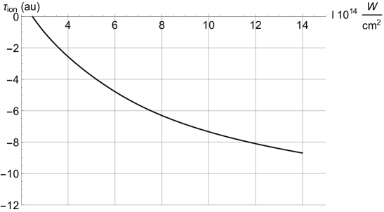
Figure 16: Ionization time as a function of the laser intensity in the 3-dimensional model (27).

We use the definition of the tunnel exit time as the moment when the quantum Hamiltonian with the electric field term removed is zero: $H_{Q}-\vec{r}\cdot\vec{E}(t)=0$. The ionization time is then defined as the difference between the time of the maximum electric field strength and the exit time, $\tau_{\rm ion}=\tau_{\rm ex}-\tau_{\rm max}$, and shown in Fig. 16. Depending on the peak laser intensity, we find an ionization time that is either positive or negative. We can easily understand this result as showing that the electron can tunnel well before the peak reaches the atom, provided the intensity of the pulse is large enough. However, a negative ionization time does not imply that there is no tunneling delay.

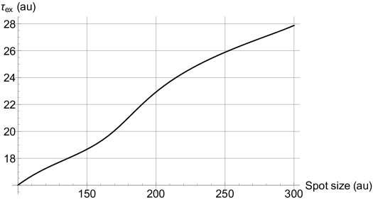
Figure 17: The exit time as a function of the spot size at a distance of 1000 atomic units.

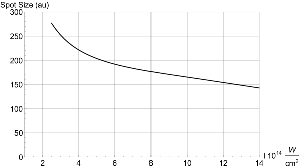
Figure 18: Spot size of the wave packet a distance of 1000 atomic units from the atom.

Other observables are also accessible as well as correlations between them. Figures 17 and 18 show that the spot size of the electron jet, defined as the geometric mean of the transversal fluctuations, depends monotonically on the exit time. This result indicates that there is indeed a tunneling delay, or at least non-trivial tunneling dynamics, even if the ionization time is negative: The larger the exit time, the more time there is for the wave packet to spread out. Additionally, the tunneling time depends monotonically on the offset angle, see Figures 19 and 20.

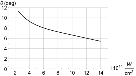
Figure 19: Off-set angle of the ionized part of the wave packet.

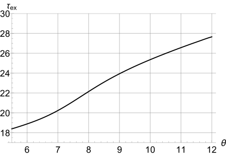
Figure 20: Tunneling exit time in terms of the offset angle.

3.6 Alternate Definition of tunneling time

The transverse fluctuations used to define the spot size have an interesting dynamics which can be used to define the tunneling exit time in an inherently quantum way, rather than using classical dynamics as in backpropagation. As indicated by Fig. 2, and confirmed below for the 3-dimensional non-static model, the transversal fluctuations have three phases. Initially, the particle is confined for some time and the fluctuations stay constant near their ground-state values. During tuneling in the second phase, the state and its fluctuations undergo a more complicated dynamics. After tunneling and when the pulse has ended, during the third phase transversal fluctuations grow linearly as is well-known for a free particle. These phases are clearly demarcated in a plot of the fluctuations, which are readily accessible from simulations in our effective potential.

Nevertheless, extracting the transverse fluctuations is not entirely trivial. To do so, we transform to the co-rotating frame in which some fluctuation parameters $s_{i}$ are transverse to the external force at all times. Under global rotations, the second-order position moments of a state, defined in general as

$$\Delta_{ij}=\langle(\hat{r}_{i}-\langle\hat{r}_{i})(\hat{r}_{j}-\langle\hat{r}_{j})\rangle\,,$$ (29)

transform in the following way

$$\bar{\Delta}_{ij}=\mathcal{O}_{ki}\Delta_{kl}\mathcal{O}_{lj}\,,$$ (30)

where $\mathcal{O}_{ij}$ is the rotation matrix that acts on position coordinates. This transformation results in the transverse fluctuation

$$s_{\rm T}=\sqrt{\cos^{2}{(\theta(t))}s_{x}^{2}+\sin^{2}{(\theta(t))}s_{y}^{2}}$$ (31)

where $\theta$ is the offset angle as a function of time.

The transversal fluctuation during the tunneling process is shown in Fig. 21, together with two linear fits of the first and final stages. The resulting tunneling exit times in Fig. 22 are less than the time of the peak at $t\approx 27$, so that we obtain negative tunneling ionization times based on this criterion, similar to Fig. 16. However, the extrapolated time in Fig. 21 lies somewhere in the middle of the second stage, and therefore does not mark the end of the tunneling process.

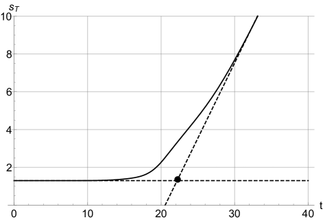
Figure 21: The transverse fluctuations as a function of time. The tangent lines of the linear regions are plotted in the dotted lines, and their intersection is marked with a dot.

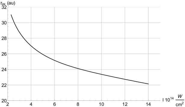
Figure 22: Alternative tunnel exit time, based on the fitting process shown in Fig. 21, as a function of the intensity.

We have to look at the tunneling dynamics in more detail in order to identify the end of tunneling. In Fig. 23 we show the second time derivative of the transversal fluctuation as a function of time, which can be interpreted as an effective force that causes the spreading. The three phases are clearly visible, with significant time dependence and a rich dynamics only in the important second phase during which tunneling happens. The time where there is a negative force is interesting, because it could be interpreted as a squeezing the particle state as it passes through the tunnel. The last local maximum and the last inflection point, indicated in the plot, are very close to the wave peak and gives the time of the maximum force on the transverse fluctuations. In particular, the last inflection point can be used as an indicator for the tunneling exit. For a range of laser intensities, the resulting tunneling exit times are shown in Fig. 24. In the entire range shown in this diagram, the exit time is greater than the time of maximum intensity at $t\approx 27$, and a positive tunneling ionization time of a few atomic units is obtained.

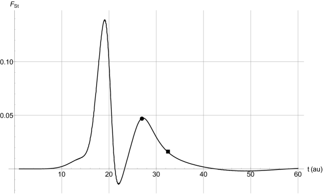
Figure 23: The effective force acting on the transverse fluctuations. We see a rich structure in the force as the particle goes through the tunneling region. The filled circle and square represent the last local maximum and the inflection point, respectively.

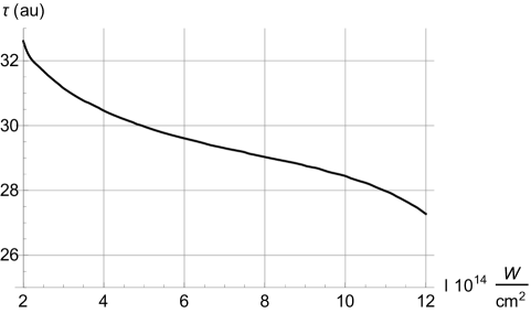
Figure 24: Tunneling time based on the last inflection point of the tunneling phase force.

4 Summary

In summary, our main result — an all-orders effective potential — makes possible a detailed analysis of the tunneling dynamics in various situations. It agrees well with observed features and is able to make new predictions. Numerical solutions give us an efficient way of generating data about the state of the electron which can be compared with observations. Our method, perhaps in combination with numerical simulations of multi-electron wave functions, can therefore be used to turn ionization experiments into indirect microscopes focused on the atomic state.

We have found qualitative agreement between our approximation and the exact Bohmian treatment. In particular, there is always a tunneling delay. One advantage of our new methods is that we have a single effective trajectory describing the quantum state through its expectation values and moments. This trajectory can directly be compared with the classical back-propagated trajectory, showing crucial deviations near the tunneling exit. In specific examples, classical back-propagation tends to underestimate the tunneling exit time. Our results therefore indicate non-zero tuneling times, but by about an order of magnitude less than what had initially been extracted from experiments. In particular, the tunneling time in a half-cycle pulse is significantly less than the tunneling time in a static field at a level of the maximum field of the pulse, which is not surprising once the importance of non-adiabatic effects has been realized [12, 17].

We also found that the definition of tunneling ionization time in non-constant fields, given by the difference of the tunneling exit time and the time of maximal field strength, does not give a full picture of the tunneling dynamics. In particular, it is possible for the electron to start tunneling well before the maximum field is reached. The entire tunneling process then takes longer than indicated by the tunneling ionization time, considered mainly in [13]. The tunneling traversal time, used in [17], gives a more complete picture of time-dependent tunneling. In our examples, we see that a tunnel opens up already at weak fields: The intensity assumed in the static example of Fig. 1 is about one tenth of the intensity used in our non-static examples, such as Fig. 8; see also Fig. 7.

Unfortunately, it is difficult to extract the full traversal time from experiments, but we have given examples of indirect signatures, such as the spot size based on fluctuations, which could be useful in this context. Moreover, if the spot size and a corresponding longitudinal fluctuation can be measured, one could use it, along with the final expectation values of position and momentum, as initial conditions for semiclassical backpropagation defined as in [12] but using our effective dynamics instead of the classical dynamics. This process would eliminate potential problems of classical backpropagation near turning points.

References

- [1] P. Eckle, A. N. Pfeiffer, C. Cirelli, et al., Attosecond Ionization and Tunneling Delay Time Measurements in Helium, Science 322 (2009) 1525–1529
- [2] N. Camus, E. Yakaboylu, L. Fechner, et al., Experimental Evidence for Quantum Tunneling Time, Phys. Rev. Lett. 119 (2017) 023201
- [3] U. S. Sainadh, H. Xu, X. Wang, et al., Attosecond angular streaking and tunnelling time in atomic hydrogen, [arXiv:1707.05445]
- [4] E. H. Hauge and J. A. Stovneng, Tunneling times: a critical review, Rev. Mod. Phys. 61 (1989) 917–936
- [5] R. Landauer and Th. Martin, Barrier interaction time in tunneling, Rev. Mod. Phys. 66 (1994) 217–228
- [6] T. Zimmermann, S. Mishra, B. R. Doran, et al., Tunneling Time in Weak Measurements in Strong Field Ionization, Phys. Rev. Lett. 116 (2016) 233603
- [7] A. S. Landsman, M. Weger, J. Maurer, R. Boge, A. Ludwig, S. Heuser, C. Cirelli, L. Gallmann, and U. Keller, Ultrafast resolution of tunneling delay time, Optica 1 (2014) 343
- [8] L. Torlina, F. Morales, J. Kaushal, et al., Interpreting attoclock measurements of tunnelling times, Nature Physics 11 (2015) 503–508
- [9] A. N. Pfeiffer, C. Cirelli, M. Smolarski, et al., Attoclock reveals natural coordinates of the laser-induced tunneling current flow in atoms, Nat. Phys. 8 (2012) 76–80
- [10] N. Eicke and M. Lein, Trajectory-free ionization times in strong field ionization, Phys. Rev. A. 97 (2018) 031402
- [11] N. Teeny, E. Yakaboylu, H. Bauke, and C. Keitel, Ionization Time and Exit Momnetum in Strong Field Tunnel Ionization, Phys. Rev. Lett. 116 (2016) 063003
- [12] H. Ni, U. Saalmann, and J.-M. Rost, Tunneling Ionization Time Resolved by Backpropagation, Phys. Rev. Lett. 117 (2016) 023002
- [13] H. Ni, U. Saalmann, and J.-M. Rost, Tunneling exit characteristics from classical backpropagation of an ionized electron wave packet, Phys. Rev. A 97 (2018) 013426
- [14] H. Ni, N. Eicke, C. Ruiz, J. Cai, F. Oppermann, N. I. Shvetsov-Shilovski, and L.-W. Pi, Tunneling criteria and a nonadiabatic term for strong-field ionization, Phys. Rev. A 98 (2018) 013411
- [15] D. Bohm, A Suggested Interpretation of the Quantum Theory in Terms of “Hidden” Variables; I, Phys. Rev. 85 (1952) 166–179
- [16] D. Bohm, A Suggested Interpretation of the Quantum Theory in Terms of “Hidden” Variables; II, Phys. Rev. 85 (1952) 180–193
- [17] N. Douguet and K. Bartschat, Dynamics of tunneling ionization using Bohmian mechanics, Phys. Rev. A 97 (2018) 013402
- [18] F. Arickx, J. Broeckhove, W. Coene, and P. van Leuven, Gaussian Wave-packet Dynamics, Int. J. Quant. Chem.: Quant. Chem. Symp. 20 (1986) 471–481
- [19] O. Prezhdo, Quantized Hamiltonian Dynamics, Theor. Chem. Acc. 116 (2006) 206
- [20] M. Bojowald and A. Skirzewski, Effective Equations of Motion for Quantum Systems, Rev. Math. Phys. 18 (2006) 713–745, [math-ph/0511043]
- [21] M. Bojowald and A. Skirzewski, Quantum Gravity and Higher Curvature Actions, Int. J. Geom. Meth. Mod. Phys. 4 (2007) 25–52, [hep-th/0606232], Proceedings of “Current Mathematical Topics in Gravitation and Cosmology” (42nd Karpacz Winter School of Theoretical Physics), Ed. Borowiec, A. and Francaviglia, M.
- [22] B. Baytaş, M. Bojowald, and S. Crowe, Faithful realizations of semiclassical truncations, arXiv:1810.12127
- [23] C. Kühn, Moment Closure—A Brief Review, In Control of Self Organizing Non-Linear Systems, pages 253–271, Springer International Publishing, 2016
- [24] B. Baytaş, M. Bojowald, and S. Crowe, Effective potentials from canonical realizations of semiclassical truncations, [to appear]
- [25] E. Wigner, The transition state method, Trans. Faraday Soc. 34 (1938) 29–41
- [26] L. V. Keldysh, Zh. Eksp. Teor. Fiz. 47 (1964) 1945, Sov. Phys. JETP 20 (1965) 1307
- [27] V. S. Popov, Tunnel and multiphoton ionization of atoms and ions in a strong laser field (Keldysh theory), Phys.-Usp. 47 (2004) 855–885