Correlated model atom in a time-dependent external field:
Sign effect in the energy shift

Abstract

In this contribution we determine the exact solution for the ground-state wave function of a two-particle correlated model atom with harmonic interactions. From that wave function, the nonidempotent one-particle reduced density matrix is deduced. Its diagonal gives the exact probability density, the basic variable of Density-Functional Theory. The one-matrix is directly decomposed, in a point-wise manner, in terms of natural orbitals and their occupation numbers, i.e., in terms of its eigenvalues and normalized eigenfunctions. The exact informations are used to fix three, approximate, independent-particle models. Next, a time-dependent external field of finite duration is addded to the exact and approximate Hamiltonians and the resulting Cauchy problem is solved. The impact of the external field is investigated by calculating the energy shift generated by that time-dependent field. It is found that the nonperturbative energy shift reflects the sign of the driving field. The exact probability density and current are used, as inputs, to investigate the capability of a formally exact independent-particle modeling in time-dependent DFT as well. The results for the observable energy shift are analyzed by using realistic estimations for the parameters of the two-particle target and the external field. A comparison with the experimental prediction on the sign-dependent energy loss of swift protons and antiprotons in a gaseous He target is made.

Dedicated to the memory of Professor Rufus Ritchie

I Introduction

The determination of the energy lost by a fast charged particle by interacting with target atoms through or near which it is passing has been the object of continuous interest. The essential featuress of the phenomenon are explained, before quantum mechanics, in terms of a classical theory due to Bohr Bohr13 . He treated the electrons near which the particle passes as classical oscillators that are set in motion by the (dipole) electric field of the heavy passing particle. The energy thus absorbed by the electrons is equal to the energy lost by the projectile. Besides this distant collision regime, close collisions were treated as pure Rutherford scattering by neglecting electron binding. However, as Fermi pointed out, quantum mechanical corrections have to be introduced for the very close impact, when the fast particle passes through a target atom Fermi40 . Close to that regime, the system of a heavy negative particle and a hydrogen atom has a critical distance at which the binding energy of the electron becomes zero. Its value is $0.639$ Bohr radii according to Fermi and Teller Teller47 . They considered the capture of negative mesotrons, i.e., negative muons ($\mu^{-}$), in matter.

Range measurements with pions ($\pi^{\pm}$), performed at around 1 MeV/amu in nuclear emulsions, predicted that the positive meson stopping power is larger than the negative pion stopping power Barkas63 . Such measurements motivated the pioneering theoretical work of the group of Ritchie Ritchie72 on the charge-sign-effect in stopping. We note that experiments, performed with protons ($Z_{1}=1$) and antiprotons ($Z_{1}=-1$) at CERN, have confirmed this charge-sign-effect in several solid-state targets over a large range of impact energies Morenzoni89 ; Moller97 .

Ritchie’s pioneering paper uses the harmonic oscillator as a model for an active electron bound in an atom and deals only with distant collision considering the dipole and quadrupole terms of the charged-projectile field. They considered their calculation as the classical equivalent of the second-order Born approximation. The subsequent, detailed quantum-mechanical calculation of Merzbacher Merzbacher74 on the same system results in agreement with that classical calculation. In one, quantum mechanical, method the dipole interaction is taken into account using a forced harmonic oscillator on which the quadrupole interaction is treated as a first-order perturbation. However, concerning the relative importance of distant and close collisions in a charge-sign effect, these calculations Ritchie72 ; Merzbacher74 prescribe different values for the minimum impact parameter below which they applied, without binding-effect, pure three-dimensional Rutherford scattering as in Bohr’s early treatment.

Motivated by these important works, in this paper, dedicated to the memory of Ritchie, we will discuss a problem beyond the common (mean-field) one-electron treatment. We would like to give a partial answer on the challenging question Quinteros91 of the interplay of an inseparable interparticle correlation and a time-dependent external excitation. In our exact treatment we will concentrate on the sign-effect in the energy shift. This attempt is highly motivated by the pioneering work of Ritchie, who used a single-electron modeling. We believe that our estimations for close-impact could have relevance not only in physics, but, maybe more importantly, in human cancer therapy Hori13 with antiproton beams as well. There the precise knowledge of the biological effectiveness is vital. Clearly, close collisions with binding-effect Kabachnik90 ; Grande97 , but without the annihilation process, could be important.

Parallel to this exciting atomistic challenge, we investigate the important problem of a harmonically confined interacting bosonic system Demler12 ; Islam15 , where the time-dependent confinement-tuning is an easily realizable experimental tool to generate correlated dynamics. Such confinement-tuning can be continuous in contrast to the discrete case with scattering of charged particles off an atom. In that, actively investigated research field of bosons the information content, like the entropies and cloud-overlaps, are in the focus of studies.

This paper is organized as follows. The next two Sections contain our target-model and the formulation of the time-dependent problem. The results, with discusions, are given in Section IV. The last Section is devoted to a short summary. We will use atomic units.

II The target: A two-particle correlated model system

As our unperturbed target, we take the interacting two-particle model first introduced by Heisenberg Heisenberg26 as one of the really simplest many-body models, and write

$$\hat{H}_{0}(x_{1},x_{2})\,=\,-\,\frac{1}{2}\left(\frac{d^{2}}{dx_{1}^{2}}\,+\frac{d^{2}}{dx_{2}^{2}}\right)+\frac{1}{2}\,\omega_{0}^{2}({x}_{1}^{2}+{x}_{2}^{2})-\frac{1}{2}\,\lambda\,\omega_{0}^{2}({x}_{1}-{x}_{2})^{2},$$ (1)

to the stationary Schrödinger equation. In Heisenberg’s classification of this Hamiltonian: it is Das denkbar einfachste Mehrkörperproblem. In Eq.(1) $\lambda\in{[0,0.5]}$ measures the strength of the allowed (see, below) repulsive interparticle interaction energy in terms of $\omega_{0}^{2}$. For $\lambda>0.5$, both interacting particles cannot both remain in the confining external field. Our exact treatment using a simple model atom will allow a useful diagnosis Cohen08 of sophisticated one-electron approximations as well. These may suffer from failures in prediction.

Introducing standard Moshinsky68 ; Davidson76 ; Pipek09 normal coordinates $X_{1}\equiv{(x_{1}+x_{2})/\sqrt{2}}$ and $X_{2}\equiv{(x_{1}-x_{2})/\sqrt{2}}$, one can easily rewrite the unperturbed Hamiltonian into the form

$$\hat{H}_{0}(X_{1},X_{2})\,=\,-\,\frac{1}{2}\left(\frac{d^{2}}{dX_{1}^{2}}\,+\frac{d^{2}}{dX_{2}^{2}}\right)+\frac{1}{2}\,\omega_{1}^{2}\,X_{1}^{2}+\frac{1}{2}\,\omega_{2}^{2}\,X_{2}^{2},$$ (2)

where $\omega_{1}\equiv{\omega_{0}}$ and $\omega_{2}\equiv{\omega_{0}\sqrt{1-2\lambda}}$ denote the frequencies of the independent normal modes. Based on Eq.(2), the normalized ground-state wave function $\Psi(X_{1},X_{2})$ is a product

$$\Psi(X_{1},X_{2})=\phi_{1}(X_{1})\phi_{2}(X_{2})\equiv{\left(\frac{\omega_{1}}{\pi}\right)^{1/4}\exp\left[-\frac{1}{2}\omega_{1}\,X_{1}^{2}\right]\,\left(\frac{\omega_{2}}{\pi}\right)^{1/4}\exp\left[-\frac{1}{2}\omega_{2}\,X_{2}^{2}\right]}.$$ (3)

Notice that $\phi_{1}(X_{1})\phi_{2}(X_{2})\neq{\phi_{1}(x_{1})\phi_{2}(x_{2})}$. We stress that the price of this normal-mode transformation is that one loses the intuitive physical picture of real particles and, instead, operates with effective independent particles representing the transformed coordinates. The ground-state energy of this model is $E=(1/2)(\omega_{1}+\omega_{2})$. There is an equal contribution from the kinetic [$(1/4)(\omega_{1}+\omega_{2})$] and potential [$(1/4)(\omega_{1}+\omega_{2})$] parts in accord with the virial theorem for bounded states. The first ionization energy is given by $\omega_{2}=\omega_{0}\sqrt{1-2\lambda}$. A formal change, $X_{1}\rightarrow{x_{1}}$ and $X_{2}\rightarrow{x_{2}}$ in Eq.(3) would correspond to a two-active-particle modeling, where, in an independent-particle picture, the ionization energies are pre-fixed.

Working with approximations at the wave-function level, we can take a product

$$\Psi_{e}(x_{1},x_{2})\,=\,\left(\frac{\omega_{e}}{\pi}\right)^{1/4}\exp\left[-\frac{1}{2}\omega_{e}\,x_{1}^{2}\right]\,\left(\frac{\omega_{e}}{\pi}\right)^{1/4}\exp\left[-\frac{1}{2}\omega_{e}\,x_{2}^{2}\right].$$ (4)

as a parametric ($\omega_{e}$) state and perform total-energy ($e$) optimization with the original Hamiltonian in Eq.(1). In fact, such an attempt is the Hartree-Fock approximation Moshinsky68 ; Davidson76 and we get Pipek09 after minimization $\omega_{e}=\omega_{0}\sqrt{1-\lambda}$ to Eq.(4). The corresponding, i.e., energetically optimal, independent-particle Hamiltonian behind $\Psi_{e}(x_{1},x_{2})\equiv{\phi_{e}(x_{1})\phi_{e}(x_{2})}$ is

$$\hat{H}_{0}^{(e)}(x_{1},x_{2})\,=\,-\,\frac{1}{2}\left(\frac{d^{2}}{dx_{1}^{2}}\,+\frac{d^{2}}{dx_{2}^{2}}\right)+\frac{1}{2}\,\omega_{e}^{2}({x}_{1}^{2}+{x}_{2}^{2}).$$ (5)

By rewriting the wave function $\Psi(X_{1},X_{2})$ in terms of physical coordinates $x_{1}$ and $x_{2}$, we determine the statistical one-matrix $\Gamma_{1}(x_{1},x_{2})$ via the following Davidson76 ; Pipek09 nonlinear mapping

$$\Gamma_{1}(x_{1},x_{2})\,=\,\int_{-\infty}^{\infty}\,dx_{3}\,\Psi^{*}(x_{1},x_{3})\,\Psi(x_{2},x_{3}).$$

From this, we arrive at an informative, i.e., Jastrow-like, representation

$$\Gamma_{1}(x_{1},x_{2})=\phi_{d}(x_{1})\,\phi_{d}(x_{2})\times{e^{-\frac{1}{2}D[(x_{1}-x_{2})]^{2}}}$$ (6)

where, with $\omega_{d}\equiv{2\omega_{1}\omega_{2}/(\omega_{1}+\omega_{2}})$, we introduced the following abbreviations

$$\phi_{d}(x)=\left[\frac{\omega_{d}}{\pi}\right]^{1/4}\,e^{-\frac{1}{2}\omega_{d}\,x^{2}}$$

$$D\,=\,\frac{1}{4}\,\frac{(\omega_{1}-\omega_{2})^{2}}{\omega_{1}+\omega_{2}}\,\geq{0}.$$

The diagonal ($x_{1}=x_{2}=x$) of the nonidempotent $\Gamma_{1}(x_{1},x_{2})$ gives the one-particle probability density, $n(x)=\Gamma_{1}(x,x)$, of unit-norm. Thus, in the knowledge of this exact result for the density $n(x)$, one may introduce the second, density-optimal ($d$), auxiliary product

$$\Psi_{d}(x_{1},x_{2})\,=\,\phi_{d}(x_{1})\phi_{d}(x_{2})\,=\,\phi_{d}(X_{1})\phi_{d}(X_{2}),$$ (7)

and associate with it an independent-particle Hamiltonian via inversion

$$\hat{H}_{0}^{(d)}(x_{1},x_{2})\,=\,-\,\frac{1}{2}\left(\frac{d^{2}}{dx_{1}^{2}}\,+\frac{d^{2}}{dx_{2}^{2}}\right)+\frac{1}{2}\,\omega_{d}^{2}({x}_{1}^{2}+{x}_{2}^{2}).$$ (8)

This Hamiltonian contains, upto an undetermined Kosugi18 constant $C_{1}(\lambda)$, the Kohn-Sham potential in the orbital implementation of Density Functional Theory Dreizler90 . One may consider such an implementation as a first-principle method based on semi-empirical inputs Cohen08 . In the knowledge of the exact ground-state energy, one could fix this constant in an inversion as $C_{1}(\lambda)\equiv{(1/4)(\omega_{0}+\omega_{2})-(1/2)\omega_{d}}=(1/4)(\omega_{0}-\omega_{2})^{2}/(\omega_{0}+\omega_{2})$, thus $C_{1}(\lambda=0)=0$.

Consider, finally, the Jastrow-like form in Eq.(6). We can apply a point-wise Riesz55 direct decomposition for it. Indeed, Mehler’s formula Erdelyi53 ; Robinson77 reads

$$(\omega_{w}/\pi)^{1/2}\,e^{-\frac{\omega_{w}}{2}\left(\frac{1+Z^{2}}{1-Z^{2}}\right)(x_{1}^{2}+x_{2}^{2})}\,e^{\omega_{w}\frac{2\,Z}{1-Z^{2}}\,x_{1}x_{2}}=\sum_{k=0}^{\infty}(1-Z^{2})^{1/2}\,Z^{k}\,\phi_{k}(\omega_{w},x_{1})\,\phi_{k}(\omega_{w},x_{2}),$$ (9)

where the parameter $Z\in{[0,1]}$, and $x_{i}\in{(-\infty,\infty)}$. The $\phi_{k}(\omega_{w},x)$ decomposition-functions form a complete set of orthonormal eigenfunctions of a one-dimensional harmonic oscillator with potential energy $\omega_{w}^{2}(x^{2}/2)$ in the Schrödinger wave equation and are given by

$$\phi_{k}(\omega_{w},x)\,=\,\left(\frac{\omega_{w}}{\pi}\right)^{1/4}\frac{1}{\sqrt{2^{k}\,k!}}\,e^{-\frac{1}{2}\omega_{w}\,x^{2}}\,H_{k}(\sqrt{\omega_{w}}x).$$ (10)

Comparison of exponentials in Eq.(6) and Eq.(9) results in the two constraints

$$(\omega_{d}+D)\,=\,\omega_{w}\,\frac{1+Z^{2}}{1-Z^{2}}$$

$$D\,=\,\omega_{w}\,\frac{2Z}{1-Z^{2}}.$$

One can solve these equations easily for $Z$ and $\omega_{w}$ in terms of $D$ and $\omega_{d}$. We get

$$Z(\lambda)\,=\,\frac{\sqrt{1+2D/\omega_{d}}-1}{\sqrt{1+2D/\omega_{d}}+1}\,=\,\left(\frac{\sqrt{\omega_{1}}-\sqrt{\omega_{2}}}{\sqrt{\omega_{1}}+\sqrt{\omega_{2}}}\right)^{2}$$

$$\omega_{w}\,=\,\omega_{d}\sqrt{1+2D/\omega_{d}}\,\equiv{\sqrt{\omega_{1}\omega_{2}}}=\omega_{0}(1-2\lambda)^{1/4}.$$

Since $\omega_{d}=\omega_{w}(1-Z)/(1+Z)$, we obtain a closed-shell-like expansion

$$\Gamma_{1}(x_{1},x_{2},\omega_{w})\,=\,\sum_{k=0}^{\infty}\,P_{k}(Z)\,\phi_{k}(\omega_{w},x_{1})\,\phi_{k}(\omega_{w},x_{2}),$$ (11)

where the occupation numbers of the natural Lowdin56 orbitals, $\phi_{k}(\omega_{w},x)$, are

$$P_{k}(Z)\,=\,(\omega_{d}/\omega_{w})^{1/2}\,(1-Z^{2})^{1/2}Z^{k}\,=\,(1-Z)Z^{k}.$$

Of course, we have $\sum_{k=0}^{\infty}P_{k}=1$. The exact result in Eq.(11) suggests our third, so-called wave-function-optimal ($w$), independent-particle modeling with $\phi_{w}(x)\equiv{\phi_{0}(\omega_{w},x)}$ in

$$\Psi_{w}(x_{1},x_{2})\,=\,\phi_{w}(x_{1})\phi_{w}(x_{2}).$$ (12)

$$\hat{H}_{0}^{(w)}(x_{1},x_{2})\,=\,-\,\frac{1}{2}\left(\frac{d^{2}}{dx_{1}^{2}}\,+\frac{d^{2}}{dx_{2}^{2}}\right)+\frac{1}{2}\,\omega_{w}^{2}({x}_{1}^{2}+{x}_{2}^{2}).$$ (13)

With the above product for $\Psi_{w}(x_{1},x_{2})$ the overlap with the exact $\Psi(x_{1},x_{2})$ is maximal variationally Nagy11 . At $\lambda\neq{0}$ we have the following ($\omega_{1}\equiv{\omega_{0}}$) ordering of frequencies:

$$\omega_{2}<\omega_{d}<\omega_{w}<\omega_{e}<\omega_{1}.$$ (14)

The ordering $\omega_{d}<\omega_{w}<\omega_{e}$ shows that the density-optimal ($d$) Kohn-Sham method and the energy optimal ($e$) Hartree-Fock method under- and overestimate the localization Cohen08 . Besides, there is an unphysical saturation in $\omega_{e}$ at the physically allowed $\lambda\rightarrow{0.5}$ limit.

Notice that one may use our normalized distribution $P_{k}$ to calculate various information-theoretic entropies (Rényi and von Neumann) or to define a normalized escort distribution as input to nonextensive (Tsallis) statistics via $P_{k}(Z)\rightarrow{P_{k}^{(q)}\equiv{P_{k}(Z^{q})}}$. Entropies measure, in our case with an interacting Hamiltonian, the deviations from independent-particle modelings, i.e., they reflect the inseparability of this Hamiltonian in original particle coordinates. They have an inherent connection with the important spectral aspect of interparticle correlation. Measuring entanglement characteristics is a recent hot topic of fundamental theoretical and practical interest in laser-field-confined cold-atom systems Demler12 ; Islam15 .

III The perturbation: a time-dependent quadrupolar field

In quantum mechanics, in the presence of an external time-dependent perturbation of finite duration, one defines the time-independent energy shift from an expectation value of the unperturbed Hamiltonian with the time-evolving state. This state is the solution of the time-dependent Schrödinger equation where one has a Cauchy problem with a prescribed initial state. In this path, the correct Ballentine98 interpretation of the effect of a time-dependent peturbation on the target-system is to produce a nonstationary state rather than to cause a jump from one stationary state to another. However, following Dirac’s method (variation of constants) to time-dependent problems, in an energy-shift calculation one can equally-well apply transition probabilities to the allowed excited states as occupation probabilities (statistical weights) to energetics. In this paper we will outline both interpretations, and demonstrate their equivalence in the determination of a time-independent energy change.

To our Hamiltonians in Eq.(1), Eq.(5), Eq.(8), and Eq.(13) we add, as excitation of $\hat{H}^{\prime}(t\rightarrow{-\infty})=\hat{H}^{\prime}(t\rightarrow{\infty})=0$ character, a time-dependent external perturbation

$$\hat{H}^{\prime}(x_{1},x_{2},t)\,=\,\frac{1}{2}\,\omega_{0}^{2}\,\Lambda\,F(t)\,({x}_{1}^{2}+{x}_{2}^{2})\equiv{\frac{1}{2}\,\omega_{0}^{2}\,\Lambda\,F(t)\,(X_{1}^{2}+X_{2}^{2})}$$ (15)

where $\Lambda$ can be positive or negative in oder to discuss the sign-effect in energy shift. Notice that in modern experiments on harmonically confined systems, with precisely specified number of atoms Islam15 , our peturbation could be considered as confinement-tuning in time. The sum of the Hamiltonians in Eq.(1) and Eq.(15) defines, mathematically, a so-called isospectral deformation of the ground-state Hamiltonian.

Since the exact Eq.(2) for two independent modes and the effective Hamiltonians in Eq.(5), Eq.(8), and Eq.(13) for two independent particles have a separable behavior in $X_{1}$ and $X_{2}$ coordinates, the addition of our separable $\hat{H}^{\prime}(X_{1},X_{2},t)$ allows simplification in mathematics. Clearly, one can consider a single oscillator [$\hat{h}(X,t)$] for which

$$\hat{h}(X,t)\,=\,-\,\frac{1}{2}\,\frac{d^{2}}{dX^{2}}\,+\frac{1}{2}\,\Omega^{2}(t)\,X^{2}.$$ (16)

where $\Omega^{2}(t)\equiv{[\Omega_{0}^{2}+\omega_{0}^{2}\,\Lambda\,F(t)]}$, and $\Omega_{0}$ is a shorthand for $\omega_{1},\omega_{2}$ and $\omega_{e},\omega_{d},\omega_{w}$. Thus, one has to solve the corresponding time-dependent Schrödinger equation

$$i\,\frac{\partial\phi(X,t)}{\partial t}\,=\,\hat{h}(X,t)\phi(X,t),$$ (17)

considering the initial condition for $\phi(X)$ at $t=-\infty$ where $\hat{h}^{\prime}(X,t)$ is zero. Our problem is one of the rare cases where it is possible to solve a nonstationary problem exactly. This mathematical exactness could be useful considering the physical statements based on it. Taking established papers Popov70 ; Kagan96 on the solution of Eqs.(16-17), we proceed along them and, similarly to these papers, we exclude the $[\Omega_{0}^{2}+\omega_{0}^{2}\,\Lambda\,F(t)]<0$ case, which may happen with certain negative $\Lambda$. Thus, in the present work, where we will use $F(t=0)=1$ as maximum below, we restrict ourselves to $|\Lambda|<(\omega_{2}/\omega_{0})^{2}=(1-2\lambda)$. An equality would mimic, at negative $\Lambda$, an ionization-like situation at $t=0$.

IV Results and discussion

The solution rests on making proper changes of the time and distance scales Popov70 ; Kagan96 to consider time-evaluation in confinement frequency. The nonstationary evolving state, denoted by $\phi[X,\Omega_{0},B,t]$, contains these scales as

$$\phi(X,\Omega_{0},B,t)=\left[\frac{\Omega_{0}}{B^{2}(t)\,\pi}\right]^{1/4}\,\exp\left[-\frac{X^{2}}{2}\,\frac{\Omega_{0}}{B^{2}(t)}\left(1-i\,\frac{B(t)\dot{B}(t)}{\Omega_{0}}\right)\right]\,e^{-i\,\gamma(t)/2},$$ (18)

where $B(\Omega_{0},t)$ and $\gamma(t)$ are interrelated in the complex solution, $\xi(t)=B(t)\exp[i\gamma(t)]$, of the following classical equation of motion

$$\ddot{\xi}(t)+\,\Omega^{2}(t)\,\xi(t)\,=\,0,$$ (19)

The nonlinear, Ermakov-type Ermakov08 ; Pinney50 differential equation, determining the real scale-function $B(t)=|\xi(t)|$ becomes

$$\ddot{B}(t)+B(t)\,\Omega^{2}(t)\,=\,B(t)[\dot{\gamma}(t)]^{2}\,=\,\frac{\Omega_{0}^{2}}{[B(t)]^{3}},$$ (20)

after taking $\dot{\gamma}(t)\equiv{\Omega_{0}/B^{2}(t)}$. The two initial conditions, reflecting the behavior of our passing excitation, are $B(t=-\infty)=1$ and $\dot{B}(t=-\infty)=0$. Notice that one could linearize this nonlinear equation in four steps by taking first $A(t)\equiv{B^{2}(t)}\neq{0}$. However, the resulting linear differential equation

$$\dddot{A}(t)+4\Omega^{2}(t)\dot{A}(t)+4\Omega(t)\dot{\Omega}(t)A(t)\,=\,0,$$

becomes a third-order one which would need three initial conditions.

Now, we illustrate the entangled nature of our correlated two-particle system in the time domain as well, similarly to the stationary case in Section II. By rewriting the exact wave function $\Psi(X_{1},X_{2},t)=\phi_{1}[X_{1},\omega_{0},B(\omega_{0},t),t]\phi_{2}[X_{2},\omega_{2},B(\omega_{2},t),t]$ in terms of original coordinates, we determine the reduced single-particle density matrix from

$$\Gamma_{1}(x_{1},x_{2},t)\,=\,\int_{-\infty}^{\infty}\,dx_{3}\,\Psi^{*}(x_{1},x_{3},t)\,\Psi(x_{2},x_{3},t),$$

After a long, but straightforward calculation we obtain

$$\Gamma_{1}(x_{1},x_{2},t)=\phi_{d}(x_{1},t)\,\phi_{d}^{*}(x_{2},t)\,\times{e^{-\frac{1}{2}D(t)(x_{1}-x_{2})^{2}}},$$

where we introduced, as a generalization of the static case, the following abbreviations

$$\phi_{d}(x,t)=\left[\frac{\omega_{d}(t)}{\pi}\right]^{1/4}\,e^{-\frac{1}{2}\omega_{d}(t)\,x^{2}[1-i\,\alpha(t)/\omega_{d}(t)]},$$ (21)

$$D(t)\,=\,\frac{1}{4}\,\frac{[\omega_{1}(t)-\omega_{2}(t)]^{2}+[\dot{B}(\omega_{1},t)/B(\omega_{1},t)-\dot{B}(\omega_{2},t)/B(\omega_{2},t)]^{2}}{\omega_{1}(t)+\omega_{2}(t)}\geq{0}$$

$$\frac{\alpha(t)}{\omega_{d}(t)}\,=\,\frac{1}{2}\,\left[\frac{B(\omega_{1},t)\dot{B}(\omega_{1},t)}{\omega_{1}}+\frac{B(\omega_{2},t)\dot{B}(\omega_{2},t)}{\omega_{2}}\right]$$

with $\omega_{d}(t)=2\omega_{1}(t)\omega_{2}(t)/[\omega_{1}(t)+\omega_{2}(t)]$, where $\omega_{i}(t)=\omega_{i}/[B(\omega_{i},t)]^{2}$ and $i=1,2$. There is mode-mixing in $\omega_{d}(t)$, $D(t)$, and $\alpha(t)$. Following our evaluation at Eqs.(6-11) in the stationary case, here we add the final form for the time-dependent occupation numbers

$$P_{k}[Z(t)]\,=\,[1-Z(t)]\,[Z(t)]^{k},$$

$$Z(t)\,=\,\frac{\sqrt{1+2D(t)/\omega_{d}(t)}-1}{\sqrt{1+2D(t)/\omega_{d}(t)}+1},$$

in terms of the time-dependent variables $D(t)$, and $\omega_{d}(t)$. This normalized distribution function could allow an analysis of time-dependent information-theoretic entropies Nagy18 .

Our nonidempotent one-matrix, with operator-trace $\mathop{\mathrm{Tr}}[\Gamma^{2}_{1}(t)]=[1+2D(t)/\omega_{d}(t)]^{-1/2}<1$, is Hermitian since $\Gamma_{1}(x_{1},x_{2},t)=\Gamma_{1}^{*}(x_{2},x_{1},t)$. Its diagonal, where $x_{1}=x_{2}=x$, gives the exact one-particle probability density $n(x,t)=\Gamma_{1}(x,x,t)$, i.e., the basic variable Dreizler86 of time-dependent DFT. The exact probability current becomes $j(x,t)=x\,n(x,t)\,\alpha(t)$ and, of course, the continuity equation of quantum mechanics is satisfied $\partial_{t}n(x,t)+\partial_{x}j(x,t)=0$. We strongly stress at this point, that in $\phi_{d}(x,t)$ , i.e., in a density- and current-optimal Kohn-Sham-like auxiliary orbital we have $\omega_{d}(t)\neq{\omega_{d}/[B(\omega_{d},t]^{2}}\equiv{\bar{\omega}_{d}(t)}$ at $t\neq{-\infty}$.

These exact probabilities are needed, in the two-particle case, to invert Lein05 a Schrödinger-like time-dependent Kohn-Sham equation for its doubly-populated orbital in order to find an effective time-dependent potential behind that auxiliary orbital $\phi_{d}(x,t)$, at least upto an undetermined time-dependent constant $C_{2}(\lambda,t)$. From such an inversion we obtain

$$V_{d}(x,t)=\frac{1}{2\sqrt{n(x,t)}}\,\partial_{x}^{2}\sqrt{n(x,t)}-\frac{1}{2}[\partial_{x}k(x,t)]^{2}-\partial_{t}k(x,t)$$

where $k(x,t)\equiv{(1/2)x^{2}\alpha(t)}$ to the polar form $\phi_{d}(x,t)=\sqrt{n(x,t)}\exp[ik(x,t)]$. The first term on the right-hand-side is an adiabatic potential which produces $n(x,t)$ as its instantaneous ground-state density. In our two-particle model with harmonic interactions, we obtain, as with Eqs.(6.50-6.52) on page 105 of Ullrich12 , for the effective potential after substitution

$$V_{d}(x,t)=\frac{1}{2}\,x^{2}\,\omega_{d}^{2}(t)\,-\frac{1}{2}\,x^{2}\sqrt{\omega_{d}(t)}\,\frac{d^{2}}{dt^{2}}\left[\frac{1}{\sqrt{\omega_{d}(t)}}\right].$$ (22)

This, formally exact, effective potential may depend Maitra15 on time even at $t\rightarrow{\infty}$, which is unphysical [see, Eq.(25) below] in the case of a perturbation with finite duration. However, starting from a pre-optimized state given by Eq.(7), and using in the above form the corresponding time-dependent frequency $\bar{\omega}_{d}(t)\equiv{\omega_{d}/[B^{2}(\omega_{d},t)]}$ instead of $\omega_{d}(t)$, we get

$$\bar{V}_{d}(x,t)=\frac{1}{2}\,x^{2}\,\left[\frac{\omega^{2}_{d}}{B^{4}(\omega_{d},t)}-\frac{\ddot{B}(\omega_{d},t)}{B(\omega_{d},t)}\right]\,\equiv{\frac{1}{2}\,x^{2}\,[\omega_{d}^{2}+\Lambda\omega_{0}^{2}F(t)]},$$

because of Eq.(20). Clearly, this potential behaves as it should physically.

Our main goal in this study is the determination of the time-independent energy shift generated by a time-dependent excitation switched on and off, i.e., which has a symmetric $\hat{H}^{\prime}(t\rightarrow{-\infty})=\hat{H}^{\prime}(t\rightarrow{\infty})=0$ character. To this determination we need the solution for $B(t)$ at the long-time limit where the the frequency is already $\Omega_{0}$. By considering the fact that Eq.(19), with $\xi(t\rightarrow{-\infty})=e^{i\Omega_{0}t}$, is mathematically equivalent Popov70 ; Kagan96 to a Schrödinger equation for the reflection coefficient $R(\Omega_{0})$ of a particle with ”energy” $\Omega_{0}^{2}$ in the ”potential” energy $-\Lambda\omega_{0}^{2}F(t)$, if $t$ is interpreted as a ”spatial coordinate”, one can Kagan96 write

$$B^{2}(\Omega_{0},t)=|\xi(t)|^{2}=\frac{1+R}{1-R}\,-\,\frac{2\sqrt{R}}{1-R}\,\cos(2\Omega_{0}t+\delta),$$ (23)

$$\gamma(t)\,=\,\arctan\left[\frac{1+\sqrt{R}}{1-\sqrt{R}}\tan(\Omega_{0}t+\delta/2)\right].$$

Of course, we have $\dot{\gamma}(t)=\Omega_{0}/B^{2}(\Omega_{0},t)$. The form in Eq.(23) is exact at $t\rightarrow{\infty}$. Clearly, once an $F(t)$ is given and the corresponding $R$ is found, we can go back to the time-evolving wave function $\phi(X,t)$ and use it to calculate energy expectation value with the time-independent Hamiltonian $\hat{h}(X)$. After subtraction from that expectation value the ground-state energy $\Omega_{0}/2$, one can find the time-independent energy shift $\Delta E(\Omega_{0})$.

It is easy to show, by applying Eq.(23) to the evolving solution in Eq.(18), that only the total energy becomes time-independent. Its kinetic and potential contributions

$$<K(t)>\,\,=\,\,\frac{\Omega_{0}}{4}\,\left[\frac{1}{B^{2}(\Omega_{0},t)}\,+\frac{\dot{B}^{2}(\Omega_{0},t)}{\Omega_{0}^{2}}\right]$$

$$<V(t)>\,\,=\,\frac{\Omega_{0}}{4}\,B^{2}(\Omega_{0},t).$$

are oscillating functions at the physically important $t\rightarrow{\infty}$ long-time limit. The one-mode, time-independent energy change takes, by using Eq.(23), a remarkably simple form

$$\Delta E(\Omega_{0})\,\equiv{\left[\frac{1}{2}\,\Omega_{0}\,\frac{1+R}{1-R}-\frac{1}{2}\,\Omega_{0}\right]}\,=\,\Omega_{0}\,\frac{R}{1-R}.$$ (24)

We stress that although $B(\Omega_{0},t)$ is an oscillating function, to energy shift we have

$$\frac{1}{4}\,\frac{1}{B^{2}(t)}\left[1+\left(\frac{B(t)\dot{B}(t)}{\Omega_{0}}\right)^{2}+B^{4}(t)\right]\,=\,\frac{1}{2}\,\frac{1+R(\Omega_{0})}{1-R(\Omega_{0})}.$$

Only this combination of $B(t)$ and $\dot{B}(t)$ will be independent of the time. Notice that using the corresponding time-independent mean values [$\bar{B^{4}}\neq{(\bar{B^{2}})^{2}}$] of our oscillating functions in the above expression, we recover the exact independent-mode result since

$$\frac{1}{4}\,\frac{1-R}{1+R}\,\left[1+\frac{2R}{(1-R)^{2}}+\frac{1+4R+R^{2}}{(1-R)^{2}}\right]\,=\,\frac{1}{2}\,\frac{1+R}{1-R}$$

When we calculate the total energy of our two-particle system, with Eq.(21) for the density-optimal wave function and Eq.(22) for the corresponding effective potential, as an expectation value in quantum mechanics, we arrive at the following

$$<E_{d}(t)>\,=\,\frac{1}{2}\,\omega_{d}(t)\left[1+\frac{\alpha^{2}(t)}{\omega_{d}^{2}(t)}\right]+\frac{1}{2}\,\omega_{d}(t)\left[1-\frac{1}{\omega_{d}^{3/2}(t)}\frac{d^{2}}{dt^{2}}\left(\frac{1}{\sqrt{\omega_{d}(t)}}\right)\right],$$ (25)

where the first expectation value is the kinetic part, and second expectation value is the potential part. This total energy is not time-independent at $t\rightarrow{\infty}$. It oscillates (at $\lambda\neq{0}$) around its mean value reflecting Maitra15 the oscillating behavior of the basic variable $n(x,t)$. One might consider this mean value (an average, based on mixed modes) as a steady-state value. But, the such-defined time-independent energy shift is not exact. Its deviation from the exact energy shift measures, a posteriori, the quality of approximations in TDDFT.

We note at this subtle point that one may argue that the $C_{2}(\lambda,t)$ constant [not determined via inversion, but $C_{2}(\lambda,t=-\infty)=C_{1}(\lambda)]$ could cure such a failure. Unfortunately, we have no rule to construct that time-dependent constant a priori, i.e., without the knowledge of the exact answer for the time-independent total energy. In complete agreement with Dreizler’s early remark Dreizler86 made at around the foundation of TDDFT, there are several reasons why the concept of universal functionals for time-dependent systems will play an even less important role in practice than in the time-independent case. We will return to this point at Eq.(35), where we calculate an action-like quantity with our exact wave function.

Now we outline briefly the second method, discussed at the beginning of Section III, which is based on transition probabilities. Interpreting these as occupation numbers one can perform a statistical averaging. These statistical weights are given by

$$W_{2n,0}(R)\,=\,\frac{(2n)!}{2^{2n}(n!)^{2}}\,\sqrt{1-R}\,(R)^{n}=\frac{1}{\sqrt{\pi}}\frac{\Gamma(n+1/2)}{\Gamma(n+1)}\sqrt{1-R}\,(R)^{n},$$ (26)

considering the allowed (by a selection rule) transitions from the ground-state Popov70 . This distribution function is normalized, i.e., $\sum_{n=0}^{\infty}W_{2n,0}(R)=1$, since

$$\frac{1}{(1-x)^{\eta}}\,=\,\sum_{n=0}^{\infty}\,\frac{\Gamma(n+\eta)}{n!\Gamma(\eta)}\,x^{n}.$$

By using this and the identity $nx^{n}=x(x^{n})^{\prime}$, the energy shift can be easily calculated as a properly weighted sum in an upward process, and the result becomes

$$\Delta E(\Omega_{0})\,=\,\Omega_{0}\,\left[\sum_{n=0}^{\infty}\,\left(2n+\frac{1}{2}\right)W_{2n,0}[R(\Omega_{0})]-\frac{1}{2}\right]\,\equiv{\Omega_{0}\,\frac{R(\Omega_{0})}{1-R(\Omega_{0})}}.$$ (27)

The equivalence of the two interpretations behind an excitation process is demonstrated.

In order to implement our exact framework, we apply an analytically solvable Landau58 ; Peierls79 textbook modeling for the time-dependence in the external field

$$F(t)\,=\,\frac{1}{\cosh^{2}(2\beta t)},$$ (28)

and calculate $R(\Omega_{0})$ of the associated ”scattering” problem discussed at Eq.(23). One can consider $(1/\beta)$ as an effective transition time. In fast, charged-particle penetration (with velocity $v$) through atomistic targets the $\beta\propto{v}$ choice seems to be a reasonable one Artacho07 . The one-mode, time-independent energy shift in Eq.(24) becomes

$$\Delta E(\Omega_{0})\,=\,\Omega_{0}\,\frac{R}{1-R}\,=\,\frac{\Omega_{0}}{\sinh^{2}[(\pi/2)(\Omega_{0}/\beta)]}\,\cos^{2}\left[(\pi/2)\sqrt{1+\Lambda\omega_{0}^{2}/\beta^{2}}\right].$$ (29)

When $\Lambda\omega_{0}^{2}/\beta^{2}<-1$, which may happen for negative $\Lambda$, one must take $\cos(iu)\Rightarrow{\cosh(u)}$. In agreement with general rules of time-dependent perturbation theory, the energy shift tends to zero in the adiabatic ($\beta\rightarrow{0}$) and sudden ($\beta\rightarrow{\infty}$) limits. This closed expression shows that the energy shift can be an oscillating function of $\Lambda>0$ at fixed $\beta$. The zeros are at $(2n+1)^{2}=[1+\Lambda(\omega_{0}/\beta)^{2}]$, where $n$ is a nonzero integer. $Z_{1}$-oscillation in the energy-loss, i.e., in energy deposition, as a function of the nuclear charge ($Z_{1}>1$) and velocity ($\beta\propto{v}$) of intruders moving in condensed matter is a challenging question Vincent06 ; Hatcher08 ; Puska14 of nonperturbative character. In our present modeling of the impact of a time-dependent perturbation the first-order, Born-like $(B)$ result corresponds to the limit of $\Lambda\rightarrow{0}$ in Eq.(29), and it becomes

$$\Delta E^{(B)}(\Omega_{0})\,=\,\left(\frac{\Lambda\omega_{0}^{2}\pi}{4\beta^{2}}\right)^{2}\,\frac{\Omega_{0}}{\sinh^{2}[(\pi/2)(\Omega_{0}/\beta)]}.$$

This perturbative result does not depend on the sign ($\Lambda$) of the external field.

In the fast-excitation, i.e., sudden limit, we get from Eq.(29) by a careful expansion

$$\Delta E(\Omega_{0})\simeq{\Omega_{0}}\,\left(\frac{\Lambda\omega_{0}^{2}}{2}\right)^{2}\,\frac{1}{(\beta\Omega_{0})^{2}}\,\left[1-\frac{1}{3}\left(\frac{\pi\Omega_{0}}{2\beta}\right)^{2}\right]\,\left(1-\frac{1}{\beta^{2}}\,\frac{\Lambda\omega_{0}^{2}}{2}\right).$$ (30)

This asymptotic form exhibits a sign effect, since $\Lambda$ can be positive or negative. However, this sign effect ($\propto{-\Lambda\omega_{0}^{2}/v^{2}}$) is opposite to the Barkas effect ($\propto{Z_{1}\Omega_{0}^{2}/v^{3}}$) found earlier Ritchie72 ; Merzbacher74 in the dipole limit with charge-conjugated particles $Z_{1}=\pm{1}$. In agreement with Fermi’s forecast Fermi40 , our theoretical result signals the importance of a quantum mechanical treatment for fast ”close collisions” with consideration ($\omega_{0}\neq{0}$) of the binding effect Kabachnik90 ; Grande97 . Such, reversed Barkas effect was predicted earlier using data sets from OBELIX experiments at CERN with swift ($v\simeq{5-6}$) protons and antiprotons moving in gaseous He, i.e., in a target of compact inert atoms Rizzini04 . We will return to this data-based prediction at Fig. 3, at the end of this section. Due to the factorized form in Eq.(29), in our three independent-particle approximations with pre-determined product states in Eq.(4), Eq.(7), and Eq.(12) we get

$$\Delta E(\Omega_{0}=\omega_{e})<\Delta E(\Omega_{0}=\omega_{w})<\Delta E(\Omega_{0}=\omega_{d}),$$ (31)

at $\beta\neq{0}$, considering the ordering of frequencies in Eq.(14) at $\lambda\neq{0}$.

Now we turn to our diagnosis. The exact expression for the total ($t$) energy shift is

$$\Delta E_{t}(\omega_{0},\omega_{2})\,=\,[\Delta E(\Omega_{0}=\omega_{0})+\Delta E(\Omega_{0}=\omega_{2})],$$ (32)

which is the sum of shifts in two independent modes. For two independent particles, constrained by different ($j=d,e,w$) inputs from the exact informations, we obtain

$$\Delta E_{t}(\omega_{j},\omega_{j})\,=\,2\,\Delta E(\Omega_{0}=\omega_{j}).$$ (33)

Furthermore, at $\beta\rightarrow{\infty}$, from Eqs.(29-32) we can deduce

$$\Delta E_{t}(\omega_{0},\omega_{2})\,=\,\Delta E_{t}(\omega_{d},\omega_{d}),$$ (34)

since $(2/\omega_{d})=(1/\omega_{0})+(1/\omega_{2})$. However, this asymptotic agreement of a density-based, i.e., Kohn-Sham-like pre-optimization procedure with the exact total energy shift, which is an observable quantity, does not allow a similar prediction for other quantities.

For instance, the exact overlap $O=|<\Psi(x_{1},x_{2})|\Psi(x_{1},x_{2},t\rightarrow{\infty})>|^{2}$ becomes

$$O=\frac{1}{\sqrt{1+\Delta E(\omega_{1})/\omega_{1}}}\frac{1}{\sqrt{1+\Delta E(\omega_{2})/\omega_{2}}}=\sqrt{1-R(\omega_{0})}\sqrt{1-R(\omega_{2})}$$

This long-time form differs (at $\lambda\neq{0}$) from the one obtained in the modeling with independent particles where $O_{d}=|<\Psi_{d}(x_{1},x_{2})|\Psi_{d}(x_{1},x_{2},t\rightarrow{\infty})>|^{2}=[1-R(\omega_{d})]$. The above form for an overlap is an important result. It is expressed in terms of scattering characteristics. From this point-of-view, it resembles to overlap-parametrizations common in many-body physics with conventional stationary scattering theory.

Notice, that in the very active research field of isolated confined cold-atom systems, with precisely specified number of atoms, an overlap $O$ seems to be an experimentally measurable quantity Demler12 ; Islam15 . In that exciting field an abrupt ($a$) change Kagan96 at $t=0$, i.e., taking the change $\Omega_{0}^{2}\Rightarrow{\Omega_{f}^{2}=(\Omega_{0}^{2}+\Lambda\omega_{0}^{2})}>0$ abruptly from the initial to the final state, we have

$$R_{a}(\Omega_{0},\Lambda)\,=\,\left[\frac{\Omega_{0}-\Omega_{f}}{\Omega_{0}+\Omega_{f}}\right]^{2}=\left[\frac{1-\sqrt{1+\Lambda(\omega_{0}/\Omega_{0})^{2}}}{1+\sqrt{1+\Lambda(\omega_{0}/\Omega_{0})^{2}}}\right]^{2}$$

Experimentally, one can produce replicas via the controllable time-dependent tuning of confinement. In such a way, we would have a series of overlaps $O(\lambda,\Lambda)$. The analysis of these overlaps might allow to deduce statements on the interparticle interaction as well. Mathematically, a two-parametric [$R(\omega_{1})$ and $R(\omega_{2})$] fitting could provide a more flexible framework than a single-parametric [$R(\omega_{d})$] one based on the mean-field concept.

Next we calculate a quantum-mechanical Berry’s connection Berry84 ; Simon83 which is defined by $\mathcal{A}(t)\equiv{i\,<\Psi(X_{1},X_{2},t)|\partial_{t}\Psi(X_{1},X_{2},t)}>$, where $i=\sqrt{-1}$. Considering the product-form of our $\Psi(X_{1},X_{2},t)$ in terms of two independent modes, we can proceed by using Eq.(18) together with Eq.(20). The one-mode ($1$) contribution to a two-term sum becomes

$$\mathcal{A}_{1}(t)=i<\phi(X,\Omega_{0},t)|\partial_{t}\phi(X,\Omega_{0},t)>=\frac{\Omega_{0}}{4}\left[\frac{\Omega^{2}(t)}{\Omega_{0}^{2}}B^{2}(t)+\frac{1}{B^{2}(t)}+\frac{\dot{B}^{2}(t)}{\Omega_{0}^{2}}\right]$$

where, as we mentioned at Eq.(16) earlier, $\Omega^{2}(t)=[\Omega_{0}^{2}+\Lambda\omega_{0}^{2}F(t)]$. At the beginning we have $\mathcal{A}_{1}(t\rightarrow{-\infty})=\Omega_{0}/2$, since at that limit $B(t)=1$ and $\dot{B}(t)=0$ due to $F(t)=0$.

This constant $\Omega_{0}/2$ value will change during the time-evolution and in the physically really important long-time limit, i.e., after perturbation, we get

$$\mathcal{A}_{1}(t\rightarrow{\infty})=\frac{\Omega_{0}}{2}\,\frac{1+R(\Omega_{0})}{1-R(\Omega_{0})}$$ (35)

which is, as expected on physical grounds, the time-independent one-mode energy given in Eq.(24)]. One gets the original value $\Omega_{0}$ even at $t\rightarrow{\infty}$ iff $R=0$, i.e., in the discrete cases discussed at Eq.(29) for the attractive situation, i.e., with $\Lambda>0$.

The mode contributions ($1$ and $2$) both will contain terms which oscillate during the action of the external field. Therefore, following the lead of an expert Simon83 , we think that it may be difficult to set up an experiment to measure (at a given time) the phase picked up by an evolving complex function when we solve an initial-value Cauchy problem using the time-dependent Schrödinger equation. Due to that, the associated action integral, on which a variational boundary-value problem in time can be based, is generally nonstationary. This problem was discussed earlier Schirmer07 by focusing on the foundation of TDDFT.

More generally, although our Cauchy problem rests on the time-dependent Schrödinger equation which contains a first-derivative in time, the time-dependent exact solution for the evolving normalized complex function requires two initial conditions to an underlying nonlinear differential equation of Ermakov-type. The linearized, equivalent, version of such a nonlinear equation would need three initial conditions. We believe that here is that mathematical complexity which may prohibit to design, without a priori informations on initial conditions or magnitudes of calculable observables, a completely predictive approximate method which is based on a Schrödinger-like auxiliary equation in orbital TDDFT.

In Figures 1 and 2 we exhibit four-four curves which were calculated at $\lambda=3/8$ and $\omega_{0}=3$, by taking $\Lambda={2/9}$ to Fig. 1, and $\Lambda=-2/9$ to Fig. 2. These figures nicely illustrate our ordering in Eq.(31). The Hartree-Fock-based curves (dotted) show the smallest energy shifts, in accord with the over-localized character of the underlying wave function. The density-based Kohn-Sham-like approximation, dash-dotted curves, gives the closest values to the exact results (solid curves). There is a crossing Nagy11 point between these curves, at around $\beta=2.86$, independently of the sign of $\Lambda$. But, despite of the under-localized character of the density-optimal independent-particle approximation, it approximates reasonably well the exact two-mode results (solid curves) which are based on different frequencies.

This, a posteriori observation supports the folklore based on the general practice with auxiliary orbitals in the mean-field TDDFT. Unfortunately, as the crossing found here signals, one can not be sure a priori about a prediction on the from-below or from-above character of numerical results. Furthermore, a comparison of magnitudes of the corresponding curves in Figs. 1-2 shows that the deviation from the exact results (solid curves) can be larger in the case of repulsion where $\Lambda<0$. This in in harmony with our expectation, based on the early results of esteemed experts Fermi40 ; Teller47 . Indeed, close to ’ionization’ a precise description is needed in order to characterize the magnitude of an observable energy shift.

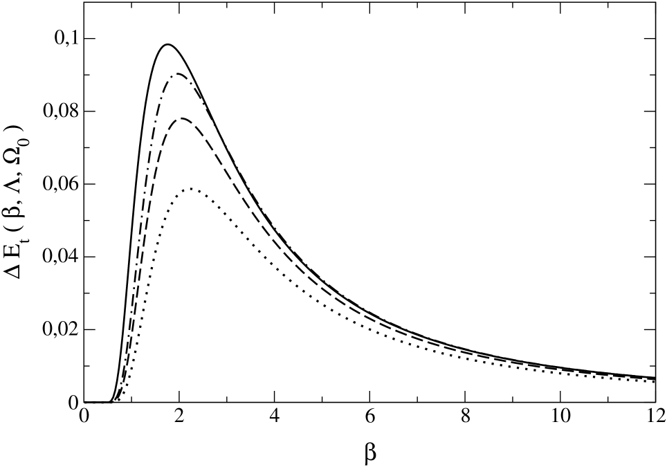
Figure 1: Total energy shifts, denoted by $\Delta E_{t}(\beta,\Lambda,\Omega_{0})$, in the attracive ($\Lambda=2/9$) case, as a function of $\beta$ at $\lambda=3/8$. Thus, the input frequencies are $\omega_{0}=3$, $\omega_{2}=1.5$, $\omega_{e}=2.372$, $\omega_{w}=2.121$, and $\omega_{d}=2$ to Eq. (29) and Eqs.(32-33). Solid curve: exact result. Dotted curve: Hartree-Fock-like approximation. Dash-dotted curve: density-optimal, Kohn-Sham-like approximation. Dashed curve: approximation based on the first natural orbital with unit occupancy. These approximations are based on pre-optimized initial states in Eq.(4), Eq.(7), and Eq.(12), respectively.

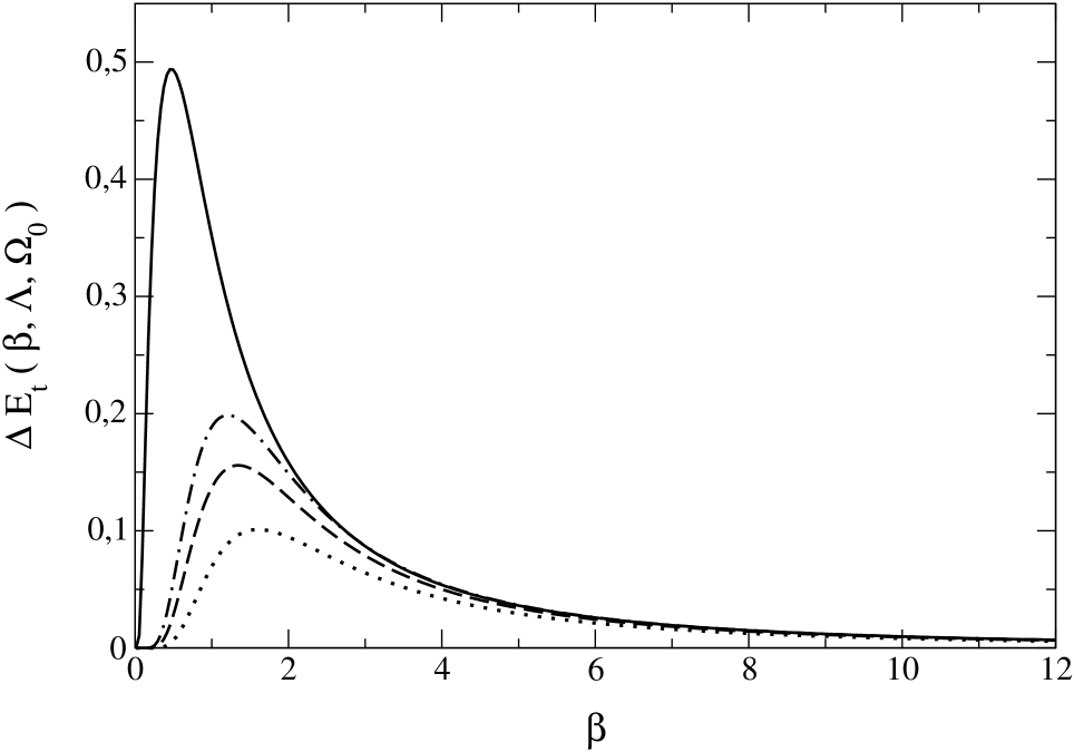
Figure 2: Total energy shifts, denoted by $\Delta E_{t}(\beta,\Lambda,\Omega_{0})$, in the repulsive ($\Lambda=-2/9$) case, as a function of $\beta$ at $\lambda=3/8$. Thus, the input frequencies are $\omega_{0}=3$, $\omega_{2}=1.5$, $\omega_{e}=2.372$, $\omega_{w}=2.121$, and $\omega_{d}=2$ to Eq. (29) and Eqs.(32-33). Solid curve: exact result. Dotted curve: Hartree-Fock-like approximation. Dash-dotted curve: density-optimal, Kohn-Sham-like approximation. Dashed curve: approximation based on the first natural orbital with unit occupancy. These approximations are based on pre-optimized initial states in Eq.(4), Eq.(7), and Eq.(12), respectively.

We mentioned at Eq.(29) that the $\beta\propto{v}$ choice ($v$ is the velocity of a fast charged intruder) seems to be a reasonable one in the sudden limit Artacho07 . As a preliminary step to future realistic calculations, here we estimate a characteristic interaction-time in classical atom-atom collision with reduced mass $\mu=M_{1}M_{2}/(M_{1}+M_{2})$. We model Nagy94 ; Arista04 the screened atom-atom interaction via a finite-range, $r\in{[0,r_{0}]}$, Mensing-type potential

$$V(r)\,=\,\frac{Z_{1}\,Z_{2}}{r}\left(1-\frac{r}{r_{0}}\right).$$

and solve the classical problem for the finite collision time ($T_{c}$) by integration. We get

$$T_{c}(b,v,r_{0})=\frac{2}{v}\left[\frac{\sqrt{r_{0}^{2}-b^{2}}}{p}+\frac{Z_{1}Z_{2}}{2E}\frac{1}{p^{3/2}}\ln\frac{\sqrt{p}\sqrt{r_{0}^{2}-b^{2}}+r_{0}+(Z_{1}Z_{2}/2E)}{\sqrt{(Z_{1}Z_{2}/2E)^{2}+p\,b^{2}}}\right]$$

where $E=\mu v^{2}/2=M_{2}/(M_{1}+M_{2})E_{1}$ is the kinetic energy. The heavy charged projectile ($Z_{1},M_{1}$) collides at impact parameter $b$ and energy $E_{1}=M_{1}v^{2}/2$ with a target atom ($Z_{2},M_{2}$) at rest. The dimensionless parameter introduced is $p=[1+(Z_{1}Z_{2}/r_{0})/E]$, i.e., it is the ratio of potential and kinetic energies. A closer inspection shows that one may apply

$$T_{c}(b,v,r_{0})\,\simeq{\alpha(v)\,\frac{r_{0}}{v}\,\frac{E}{E+Z_{1}Z_{2}/r_{0}}}\,\sqrt{1-\frac{b^{2}}{r_{0}^{2}}}$$

to get a reasonable estimation as a function of the heavy projectile velocity $v$. The $\alpha(v)$ parameter decreases from 4 (at $v\rightarrow{0}$) to 2 (at $v\rightarrow{\infty}$). A cross-sectional average becomes

$$\bar{T}_{c}(v,r_{0})=\alpha(v)\,\frac{r_{0}}{3v}\,\frac{E}{E+Z_{1}Z_{2}/r_{0}}.$$

In this simple modeling of the nuclear ($Z_{1}Z_{2}>0$) elastic collision we are at the sudden situation ($\bar{T}_{c}\rightarrow{0}$) for both limits of the intruder velocity $v$.

In particular, our asymptotic form in Eq.(30) would give, with the natural choice of $2\beta=(1/\bar{T}_{c})$, a quadratic behavior $\Delta E(\Omega_{0})\propto{v^{2}}$ at small enough velocities. Such an energy shift can be much smaller than the energy difference ($\sim{\Omega_{0}}$) between the unperturbed states. However, a time-dependent excitation process is a rigorously quantum mechanical process since, classically, this energy shift is not enough to make a single-particle jump for which one could take conservation laws of two-body kinematics as the only decisive constraints.

In Figure 3, we plot the ratio $\{[\Delta E_{t}(\Lambda=-2/9)/\Delta E_{t}(\Lambda=2/9)]-1\}$ as a function of the velocity for which we take for simplicity $v=\beta$. This corresponds to a quasiclassical Thomas-Fermi-like choice $r_{0}=3/4\simeq{1/Z_{2}^{1/3}}$ (with $Z_{2}=2$) to be used in the above high-velocity form. The corresponding results are plotted for $v\in[4,12]$. One can see that the plotted difference approaches zero, as expected on physical grounds, by increasing the velocity. At the lower range (still swift antiprotons or protons, with bombarding energy about $E_{1}=400-500$ keV) the difference can be in the $10\%$ range. This magnitude is not in contradiction with the estimation ($15\pm{5}\%$, at that energies) based on OBELIX stopping data obtained Rizzini04 at CERN for a gaseous He target ($Z_{2}=2$) with $Z_{1}=\pm{1}$.

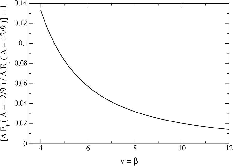
Figure 3: The exact ratio in form of $\{[\Delta E_{t}(\Lambda=-2/9)/\Delta E_{t}(\Lambda=2/9)]-1\}$ as a function of the velocity $v$ for which we take $v=\beta$. In our parametrization we have $(\Lambda\omega_{0}^{2}/2)={\pm{1}}$.

We left a more detailed investigation of the energy shift, by using an impact parameter dependent estimation for the collisional time $T_{c}(b,v,r_{0})$, for a future study. Such a study, combined with estimations for the distant (large impact parameter) range, where the polarization-related energy shift generated by a dipole-like field may be important Kabachnik90 , is highly desirable for an interacting system. Furthermore, one should keep in mind that contributions from the nuclear-stopping and electronic-stopping are evidently correlated Sigmund08 . In our case, a simple re-parametrization with $r_{0}(v)>r_{0}$ would change the original partial stopping calculated at $r_{0}$. At high velocities both, nuclear and electronic, contributions could be larger due to their scaling $\propto{[r_{0}(v)]^{2}}$. Consistent attempts Correa12 are desirable.

V Summary

In this contribution we determined the exact solution for the ground-state wave function of a two-particle correlated model atom with harmonic interactions. The model was introduced by Heisenberg and constitutes a cornerstone in such areas of physics, as the field of correlated atoms and confined quantum matter. Next, a time-dependent external field of finite duration is addded to the Hamiltonian and the resulting Cauchy problem is solved. The impact of this external field is investigated by calculating the energy shift in the model atom. It is found that the nonperturbative energy shift reflects the sign of the driving field. Three independent-particle approximations, defined from exact informations on the correlated model, are investigated as well in order to understand their limitations.

Paralell to the investigation of the sign-effect in an energy shift, we determined and analyzed other measures of an inseparable two-body problem, namely the overlap and a Berry’s connection which are also based on the precise wave function. To our best knowledge, the overlap seems to be a measurable quantity in modern experiments with confined cold atoms of controllable number. Unfortunately we can not see, at this moment at least, an experimental tool to measure Berry’s connection in our time-dependent problem.

But, to be optimistic at this alarming point as well, we would like to refer to the wish of the Duke of Gloucester in one of Shakespeare’s famous plays. I can add colours to the chameleon – emphasized the Duke in his monologue. We believe that by the application of carefully selected experimental and theoretical tools, finally one can get a transferable knowledge on an observable ’chameleon’ by focusing on its really visible ’colours’.

- (1) N. Bohr, Phil Mag. 25, 10 (1913); P. Sigmund, Phys. Rev. A 54, 3113 (1996).
- (2) E. Fermi, Phys. Rev. 57, 485 (1940).
- (3) E. Fermi and E. Teller, Phys. Rev. 72, 399 (1947).
- (4) W. H. Barkas, J. W. Dyer, and H. Heckman, Phys. Rev. Lett. 11, 26 (1963).
- (5) J. C. Ashley, R. H. Ritchie, and W. Brandt, Phys. Rev. B 5, 2393 (1972).
- (6) K. W. Hill and E. Merzbacher, Phys. Rev. A 9, 156 (1974).
- (7) L. H. Andersen, H. Hvelpund, H. Knudsen, S. P. Moller, J. O. P. Pedersen, E. Uggerhoj, K. Elsener, and E. Morenzoni, Phys. Rev. Lett. 62, 1731 (1989).
- (8) S. P. Moller, E. Uggerhoj, H. Blume, H. Knudsen, U. Mikkelsen, K. Paludan, E. Morenzoni, Phys. Rev. A 56, 2930 (1997).
- (9) T. B. Quinteros and J. F. Reading, Nucl. Instrum. Methods B 53, 363 (1991).
- (10) M. Hori and J. Walz, Prog. Part. Nucl. Phys. 72, 206 (2013).
- (11) L. L. Balashova, N. M. Kabachnik, and V. N. Kondratev, Phys. Stat. Sol. (b) 161, 113 (1990).
- (12) P. L. Grande and G. Schiwietz, Nucl. Instrum. Methods B 132, 264 (1997).
- (13) D. Abanin and E. Demler, Phys. Rev. Lett. 109, 020504 (2012).
- (14) R. Islam, R. Ma, P. M. Preiss, M. Eric Tai, A. Lukin, M. Rispoli, and M. Greiner, Nature 528, 77 (2015).
- (15) W. Heisenberg, Z. Phys. 38, 411 (1926).
- (16) A. J. Cohen, P. Mori-Sánchez, and W. Yang, Science 321, 792 (2008).
- (17) M. Moshinsky, Am. J. Phys. 36, 52 (1968).
- (18) E. R. Davidson, Reduced Density Matrices (Academic Press, New York, 1976).
- (19) J. Pipek and I. Nagy, Phys. Rev. A 79, 052501 (2009).
- (20) T. Kosugi and Y.-I. Matsushita, J. Phys.: Condens. Matter 30, 435604 (2018).
- (21) R. M. Dreizler and E. K. U. Gross, Density Functional Theory (Springer-Verlag, Berlin, 1990).
- (22) F. Riesz and B.-Sz. Nagy, Functional Analysis (Ungar, New York, 1955).
- (23) A. Erdélyi, Higher Transcendental Functions (McGraw-Hill, New York, 1953), p. 194.
- (24) P. D. Robinson, J. Chem. Phys. 66, 3307 (1977).
- (25) P.-O. Löwdin and H. Shull, Phys. Rev. 101, 1730 (1956).
- (26) I. Nagy and I. Aldazabal, Phys. Rev. A 84, 032516 (2011).
- (27) L. E. Ballentine, Quantum Mechanics (World Scientific, Singapore, 1998).
- (28) V. S. Popov and A. M. Perelomov, Sov. Phys. JETP 29, 738 (1969); ibid 30, 910 (1970).
- (29) Yu. Kagan, E. L. Surkov, and G. V. Shlyapnikov, Phys. Rev. A 54, R1753 (1996).
- (30) V. P. Ermakov, Appl. Anal. Discrete Math. 2, 123 (2008).
- (31) E. Pinney, Proc. Amer. Math. Soc. 1, 681 (1950).
- (32) I. Nagy, J. Pipek, and M. L. Glasser, Few-Body Syst. 59, 2 (2018).
- (33) H. Kohl and R. M. Dreizler, Phys. Rev. Lett. 56, 1993 (1986).
- (34) M. Lein and S. Kümmel, Phys. Rev. Lett. 94, 143003 (2005).
- (35) C. A. Ullrich, Time-Dependent Density-Functional Theory (University Press, Oxford, 2012).
- (36) J. I. Fuks, K. Luo, E. D. Sandoval, and N. T. Maitra, Phys. Rev. Lett. 114, 183002 (2015).
- (37) R. Vincent and I. Nagy, Phys. Rev. B 74, 073302 (2006).
- (38) R. Hatcher, M. Beck, A. Tackett, and S. T. Pantelides, Phys. Rev. Lett. 100, 103201 (2008).
- (39) A. Ojanperä, A. V. Krasheninnikov, and M. Puska, Phys. Rev. B 89, 035120 (2014).
- (40) L. D. Landau and E. M. Lifshitz, Quantum Mechanics (Pergamon Press, London, 1958).
- (41) R. Peierls, Surprises in Theoretical Physics (Princeton University Press, Princeton, 1979).
- (42) E. Artacho, J. Phys.: Condens. Matter 19, 275211 (2007).
- (43) E. Lodi Rizzini et al, Phys. Lett. B 599, 190 (2004).
- (44) M. V. Berry, Proc. R. Soc. London, Ser. A 392, 45 (1984).
- (45) B. Simon, Phys. Rev. Lett. 51, 2167 (1983).
- (46) J. Schirmer and A. Dreuw, Phys. Rev. A 75, 022513 (2007).
- (47) I. Nagy, Nucl. Instrum. Methods B 94, 377 (1994).
- (48) N. R. Arista, P. L. Grande, and A. F. Lifschitz, Phys. Rev. A 70, 042902 (2004).
- (49) P. Sigmund, Bull. Russ. Acad. Phys. 72, 569 (2008).
- (50) A. A. Correa, J. Kohanoff, E. Artacho, D. Sánchez-Portal, and A. Caro, Phys. Rev. Lett. 108, 213201 (2012).