Explicit Feedbacks Meet with Implicit Feedbacks : A Combined Approach for Recommendation System

Abstract

Recommender systems recommend items more accurately by analyzing users’ potential interest on different brands’ items. In conjunction with users’ rating similarity, the presence of users’ implicit feedbacks like clicking items, viewing items specifications, watching videos etc. have been proved to be helpful for learning users’ embedding, that helps better rating prediction of users. Most existing recommender systems focus on modeling of ratings and implicit feedbacks ignoring users’ explicit feedbacks. Explicit feedbacks can be used to validate the reliability of the particular users and can be used to learn about the users’ characteristic. Users’ characteristic mean what type of reviewers they are. In this paper, we explore three different models for recommendation with more accuracy focusing on users’ explicit feedbacks and implicit feedbacks. First one is $RHC-PMF$ that predicts users’ rating more accurately based on user’s three explicit feedbacks (rating, helpfulness score and centrality) and second one is $RV-PMF$, where user’s implicit feedback (view relationship) is considered. Last one is $RHCV-PMF$, where both type of feedbacks are considered. In this model users’ explicit feedbacks’ similarity indicate the similarity of their reliability and characteristic and implicit feedback’s similarity indicates their preference similarity. Extensive experiments on real world dataset, $i.e.$ Amazon.com online review dataset shows that our models perform better compare to base-line models in term of users’ rating prediction. $RHCV-PMF$ model also performs better rating prediction compare to baseline models for cold start users and cold start items.

1 Introduction

In various domains like E-commerce platforms, online news, online movie sites etc., recommender system performs an important role in attenuating information overburden, having been notoriously adopted. Based on information of demographic profiles and previous preferences of users, recommender systems [11] predict users’ rating or purchasing decision of items and recommend right items or right news or suitable friends to the interested users based on prediction. Most of the existing recommendation approaches could be mainly categorized into Content-Based approach [9] and Collaborative Filtering ($CF$) approach [12]. Memory Based method [15] and Model Based method [5] are two categories of $CF$.

To learn high quality user-item embedding, researchers are considering various side informations related to users’ implicit feedbacks, user-item interactions [2], product reviews [4, 14] and product images [10], that lead to better rating prediction. A user purchases an item based on her preference or influenced by others. After purchasing the item, the user gives positive (good) or negative (bad) rating based on her satisfaction level. There are different types of reviewers in online merchandise sites such as positive reviewers, critical reviewers or reliable reviewers. As for example, if any user gives bad rating for her purchasing item and more number of users click her review as “helpful yes”, that means she is not only a critical reviewer but also a reliable reviewer because more number of users support her review and rating. Considering for another case if more number of users click her review as “ helpful no”, that means she is only a critical reviewer but not a reliable one.

In our method, high helpfulness score and centrality score with positive rating (company should fix threshold value for rating) means the user is not only a positive reviewer but also a reliable reviewer and low helpfulness score and low centrality score with positive rating means the user is only a positive reviewer. Similarly, high helpfulness score and high centrality score with negative rating means the user is not only a critical reviewer but also a reliable reviewer and low helpfulness score and low centrality score with negative rating means the user is only a negative or critical reviewer. The company should fix the threshold value to define high, low score range and positive or negative rating range. In [2, 4, 10, 14] authors are focusing on only implicit feedbacks like user-item interactions, users’ view similarity, product images etc. that lead to better user’s preference prediction not rating prediction because a user’s rating prediction depends on what type of reviewer she is: positive reviewer or critical reviewer or reliable reviewer. These type of characteristic, we easily predict from user’s explicit feedbacks’ similarity. They ignore users’ explicit feedbacks that indicate users’ characteristic.

In our research, we consider three explicit feedbacks like ratings, helpfulness score and centrality score and one implicit feedback like view relationship with user-item. From implicit feedback, we can predict a user’s preference areas more accurately and from explicit feedbacks we can guess the user’s predicted rating on her preferred items more accurately. The online merchandise company should recommend such items to a user who not only purchases the item based on her preference but also gives good rating because a user’s negative rating or review always affects financial health of a company.

If a user’s (positive reviewer) helpfulness score and centrality score is similar to the particular users whose helpfulness score and centrality score are high and rating is positive, that means the user is a positive and a reliable reviewer and her rating activity will be similar to other positive and reliable reviewers. Similarly, if a user’s (critical reviewer) helpfulness score and centrality score is similar to the particular users whose helpfulness score and centrality score are high and rating is negative, that means the user is a critical and reliable reviewer and her rating activity will be similar to other critical and reliable reviewers. For another case, if a user’s helpfulness score and centrality score is similar to the particular users whose helpfulness score and centrality score are low with positive or negative rating, that means the user is only positive or critical reviewer, respectively. So, based on explicit feedbacks similarity, we can predict more accurately a user’s characteristic, that helps us to predict her rating activity and implicit feedback similarity helps us to predict a user’s preference areas. If we consider both explicit and implicit feedback similarity, then we can predict a user’s characteristic and preference area both more accurately that help us to predict her ratings activity more precisely.

The rest of the paper is organized as follows: In section 2, we describe our methodology that contains, Probabilistic Model ($RHC-PMF$) on explicit feedbacks, Probabilistic Model ($RV-PMF$) on implicit feedback, and the fusion of explicit feedbacks and implicit feedback. In section 3, we show performance of our proposed models and in section 4, we give conclusion and future work.

2 Methodology

Explicit Feedback : In this paper, we consider three explicit feedbacks such as user’s rating, helpfulness score and centrality score.

i) Rating Scores : In online merchandise site a user gives rating on her purchased item. We denote $R_{ij}$ as the rating of user $U_{i}$ for item $P_{j}$. For example, Amazon.com ratings span is from $1$ to $5$. In this paper, we follow the same rating scale. Rating $1$, $2$ are considered as negating rating and $3$ to $5$ are mentioned as positive rating.

ii) Helpfulness Score : Before purchasing an item users are expected to read the previous reviews regarding the particular item. In most of the merchandise sites after each review, it asks the question, “Was this review helpful to you? (Answer Yes/No)”. “Yes” answer indicates that the review is helpful to the user. “No” answer indicates that the review is not proper or not truthful. This helpfulness data can be used to validate the reliability of the particular user’s item review.

We define a new formula to evaluate helpfulness score $H_{ij}$ of the review given by user $U_{i}$ for item $P_{j}$ as follows:

$$H_{ij}=(-1)^{\theta}\frac{x_{ij}^{2}}{y_{ij}},$$ (1)

where $x_{ij}$ is the number of users who marked the review given by user $U_{i}$ for item $P_{j}$ as helpful and $y_{ij}$ is the total number of users who have answered that question (total count of yes and no). If $R_{ij}$ is in the range of [ +3, +5 ], $\theta$ is equal to 2, otherwise 1. The above equation is quadratic in nature because we want to give more priority to the particular users who have more number of “yes click”. Helpfulness score with positive sign indicates that the user is a positive reviewer and negative sign indicates that the user is a critical reviewer. It is very difficult to get the exact information about the users who not only marked the review as helpful but also purchase the item. So we do not consider this scenario. We assume that the users who marked the review as helpful are interested to purchase the item. In the real world, there are many users who read the reviews of previous users but do not click on helpful “yes” or “no”. Our experimental dataset does not provide such type of information. So, it is out of our consideration.

iii) Review Network and Centrality Score :

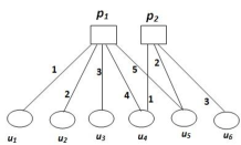
Figure 1: Bipartite network between items and users. An edge denotes a review is written by a user on an item.

When we are going to purchase any item from online merchandise sites, we read previous customers’ reviews which are related to that particular item. We can build a network of reviewers based on their purchasing items and timestamps. We name this network as Review Network[16].

Fig. 1 depicts a bipartite network presenting the review data set. Two sets of nodes in that bipartite network are item set and user set. If user $U_{i}$ writes a review on item $P_{j}$ then there will be an edge between them. Essentially each edge represents a distinct review. Notice that, each review has a time stamp of its creation. We identify each edge by a unique number that indicates logical time stamp of edge creation. Please note that in this figure we have not specified original time stamps. For depiction purpose, we have assumed some time direction in Fig. 1. The edges between user $U_{1}$ - item $P_{1}$ and user $U_{2}$ - item $P_{1}$ are identified by time stamp $1$ and $2$ respectively, that means user $U_{2}$ posts her rating after user $U_{1}$. According to the review post timing, here we assume that user $U_{2}$ purchases the item after user $U_{1}$. In Fig. 1, $P_{1}$, $P_{2}$ are items and $U_{1}$, $U_{2}$, $U_{3}$, $U_{4}$, $U_{5}$, $U_{6}$ are users who have written reviews on one or two items.

In this paper, we use degree centrality to evaluate centrality score of each user for a particular item in review network. We evaluate a user’s centrality score based on how many other users read her review. Our dataset does not provide exact information about the users who read others reviews regarding a particular item. When a user wants to read the previous reviews of other users for a particular item, in online merchandise site there are two option : a) Most recent reviews b) Top ranking reviews. Based on our realistic assumption, centrality score of each user is evaluated.

Most recent reviews are selected based on current time stamp and the time stamp when the users post reviews. Based on most recent reviews centrality score ($most_{ij}$) of user $U_{i}$ for item $P_{j}$ is evaluated from our proposed equation:

$$most_{ij}=\sum_{r=1}^{n-i}\dfrac{1}{r},$$ (2)

where $n$ is total number of users who purchase item $P_{j}$. $i$ starts from 1 means $U_{1}$ is the first user who purchases item $P_{j}$. As for example, in Fig. 1 $U_{1}$ is the first user who writes review regarding item $P_{1}$. Before purchasing the same item, $U_{2}$ reads $U_{1}$’s review as most recent review and for $U_{2}$, $U_{1}$’s centrality score = 1. When $U_{3}$ purchases the same item, she may read $U_{1}$’s review as second most recent review and for $U_{3}$, $U_{1}$’s centrality score = 1/2. Total centrality score of $U_{1}$ user for item $P_{1}$ = $\sum_{r=1}^{4}\dfrac{1}{r}$.

Now we consider centrality score of users based on top ranking reviews. We evaluate top ranking reviews based on their helpfulness score for all positive reviewers and all critical reviewers separately from our proposed equation :

$$top_{ij}=(\dfrac{1}{k_{i}})^{2}*(n-i),$$ (3)

where, $top_{ij}$ is the centrality score of user $U_{i}$ for item $P_{j}$ based on top ranking review. $k_{i}$ is the ranking for user $U_{i}$. Higher helpfulness score means rank is higher. $(n-i)$ indicates how many users purchase the same item after $i^{th}$ user.

Total centrality score $D_{ij}$ is calculated based on our proposed technique as follows:

$$D_{ij}=(-1)^{\theta}\times(\alpha*top_{ij}+(1-\alpha)*most_{ij}),$$ (4)

where $\alpha$ is weightage value. The company’s management would decide the exact weightage value. Here we set weightage = 0.5. If $R_{ij}$ is in the range of [ +3, +5 ], $\theta$ is equals to 2, otherwise 1. Centrality score with negative sign indicates that the user is critical reviewer and positive sign for positive reviewer.

Implicit Feedback : In this paper, we consider view relationship as implicit feedback between user-item to predict a user’s preference areas more accurately.

i) View Relationship : Before purchasing any item, users always view different items on the same category based on their preference areas. The online merchandise sites have information about the view history of registered users, that helps us to understand the preference area of a user. Based on this information, recommender system recommends items to users based on their interest.

Probabilistic Model with Explicit Feedbacks (RHC-PMF) :

In this section, we first describe how ratings $R$ is approximated by helpfulness score $H$ and centrality scores $D$. In this section, we introduce user-item rating matrix. Typically there are three type of objects, namely users, ratings and items. Suppose, $U$ = $\{$ $U_{1}$, $U_{2}$, …., $U_{n}$ $\}$ be the set of users, ${P}$ = $\{$ $P_{1}$, $P_{2}$, …., $P_{m}$ $\}$ be the set of items, ${R}$ = $\{$ $R_{1}$, $R_{2}$, …., $R_{N}$ $\}$ be the set of ratings, ${H}$ = $\{$ $H_{1}$, $H_{2}$, …., $H_{N}$ $\}$ be the set of helpfulness scores and ${D}$ = $\{$ $D_{1}$, $D_{2}$, …., $D_{N}$ $\}$ be the set of centrality scores where $n,m$ are the number of users and items respectively. $N$ is the number of rating, helpfulness score and centrality individually.

We use the matrix $R$ = [$R_{ij}$]_n×m $\in$ $\mathbb{R}^{n\times m}$ to indicate the user-item rating matrix produced by the users who give ratings on different purchasing items, where $R_{ij}$ is the rating score that is given by user $U_{i}$ on item $P_{j}$. Similarly, the matrix $H$ = [$H_{ij}$]_n×m $\in$ $\mathbb{R}^{n\times m}$ to indicate the user-item helpfulness score based matrix gained by the users on different purchasing items, where $H_{ij}$ is the helpfulness score that is scored by user $U_{i}$ on item $P_{j}$. Another matrix $D$ = [$D_{ij}$]_n×m $\in$ $\mathbb{R}^{n\times m}$ to indicate the user-item centrality score based matrix gained by the users on different purchasing items, where $D_{ij}$ is centrality score that is scored by user $U_{i}$ on item $P_{j}$.

Our method try to factorize the rating matrix $R$ $\in$ $\mathbb{R}^{n\times m}$ into two matrices $W$ $\in$ $\mathbb{R}^{K\times n}$ and $Z$ $\in$ $\mathbb{R}^{K\times m}$. $W$ is the user latent factor matrix with each column $W_{i}$ being $W_{i}$’s latent feature vector that indicates how user $U_{i}$’s taste is similar to other users based on ratings and $Z$ is the item latent factor matrix with each column $Z_{j}$ being the latent feature vector of the item $P_{j}$ that indicates how the other users rate on item $P_{j}$. The helpfulness score based matrix $H$ $\in$ $\mathbb{R}^{n\times m}$ is also factorized into two matrices $E$ $\in$ $\mathbb{R}^{K\times n}$ and $F$ $\in$ $\mathbb{R}^{K\times m}$ where, $E$ is the user latent factor matrix with each column $E_{i}$ being $E_{i}$’s latent feature vector that indicates how user $U_{i}$’s helpfulness score is similar to other users and $F$ is the item latent factor matrix with each column $F_{j}$ being the latent feature vector of the item $P_{j}$ that indicates how the other users get helpfulness score on item $P_{j}$. Similarly, the centrality score based matrix $D$ $\in$ $\mathbb{R}^{n\times m}$ is factorized into two matrices $C$ $\in$ $\mathbb{R}^{K\times n}$ and $O$ $\in$ $\mathbb{R}^{K\times m}$. Here we consider users’ explicit feedbacks like ratings, helpfulness score and centrality and try to represent each user and item by a low-dimensional vector. MF tries to map both users and items to a joint latent factor space with low-dimensionally $K$ such that user-item interactions are modeled as inner items in that space.

We define the conditional distribution  [8] over the observed ratings as:

$$\begin{split}p(R|W,Z,\sigma_{R}^{2})=\prod_{i=1}^{n}\prod_{j=1}^{m}\bigg{[}\mathcal{N}\bigg{(}R_{ij}|g(W_{i}^{T}Z_{j})\bigg{)},\sigma_{R}^{2}\bigg{]}^{I_{ij}^{R}},\end{split}$$ (5)

where $\mathcal{N}(x|\mu,\sigma^{2})$ denotes the probability function of a Gaussian distribution with mean $\mu$ and variance $\sigma^{2}$. $I_{ij}^{R}$ is equal to 1 if user $U_{i}$ rated item $P_{j}$, and 0 otherwise. Tanh function $g(.)$ is used to map the range of $(W_{i}^{T}Z_{j})$ within [-1,+1], and we map $R_{ij}$ into the same range [-1,+1] using the following Eq. 6.

$$x^{\prime}=c+(x-a)\bigg{(}\dfrac{d-c}{b-a}\bigg{)},$$ (6)

where x is a value into an interval [a,b] and we have to map it into an interval [c,d]. $x^{{}^{\prime}}$ is scaled value of x into the interval [c,d].

For each hidden variable, we place zero-mean spherical Gaussian priors [1] as follows :

$$\begin{split}p(W|\sigma_{W}^{2})=\prod_{i=1}^{n}\mathcal{N}\bigg{(}W_{i}|\ 0,\dfrac{\sigma_{W}^{2}}{n_{w_{i}}}\textbf{I}\bigg{)}\ and\ p(Z|\sigma_{Z}^{2})=\prod_{j=1}^{m}\mathcal{N}\bigg{(}Z_{j}|\ 0,\dfrac{\sigma_{Z}^{2}}{n_{z_{j}}}\textbf{I}\bigg{)}\end{split}$$ (7)

Please note that, we do not consider a uniform variance of all users as shown in Eq.7. We try to make more reasonable to characterize different users with different prior variance for better recommendation. Here $n_{w_{i}}$ is the number of ratings given by user $U_{i}$ means we have to adjust user $U_{i}$’s prior variance according to $n_{w_{i}}$. The more number of ratings given by user will contribute more accuracy to learn her rating activity and consequently, the smaller the uncertainty. This means that the prior variance of user $U_{i}$ will be inversely proportional to $n_{w_{i}}$. $n_{z_{j}}$ is the number of users who rate on item $P_{j}$.

Similar as Eq. 5, 7 we have defined the another conditional distribution over the observed helpfulness score, that is $p(H|E,F,\sigma_{H}^{2})$, where $p(E|\sigma_{E}^{2})$ and $p(F|\sigma_{F}^{2})$, the priors of the user and item features based on helpfulness score, are modeled as zero-mean spherical Gaussian distribution. Due to space limitation, expressions are omitted. Here $H_{ij}$ is also mapped into the range [-1, +1] using Eq. 6. Similarly, here we do not consider a uniform variance. Another conditional distribution over the observed centrality score is $p(D|C,O,\sigma_{D}^{2})$ where $p(C|\sigma_{C}^{2})$ and $p(O|\sigma_{O}^{2})$, the priors of the user and item features based on centrality score, are modeled as zero-mean spherical Gaussian distribution.

In our model user vector $W_{i}$ based on rating approximates to the user vector $E_{i}$ based on helpfulness score. So, we define a conditional distribution of $W_{i}$ given $E_{i}$ as follows:

$$\begin{split}p(W|E,\sigma_{WE}^{2})=\prod_{i=1}^{n}\mathcal{N}\bigg{(}W_{i}|\ E_{i},{\sigma_{WE}^{2}}\textbf{I}\bigg{)},\end{split}$$ (8)

where variance $\sigma_{WE}^{2}$ controls the extent by which $W_{i}$ approximates $E_{i}$. Similarly, we define another conditional distribution of $W_{i}$ given $C_{i}$, that is $p(W|C,\sigma_{WC}^{2})$, where variance $\sigma_{WC}^{2}$ controls the extent by which user vector $W_{i}$ based on rating approximates $C_{i}$ based on centrality score.

Now, we can compute the posterior distribution over the hidden variables considering three explicit feedbacks:

$$\begin{split}p(W,Z,E,F,C,O|R,H,D,\sigma_{R}^{2},\sigma_{H}^{2},\sigma_{D}^{2},\sigma_{WE}^{2},\sigma_{WC}^{2},\sigma_{W}^{2},\sigma_{Z}^{2},\sigma_{E}^{2},\sigma_{F}^{2},\sigma_{C}^{2},\sigma_{O}^{2})\propto\\ p(R|W,Z,\sigma_{R}^{2})p(H|E,F,\sigma_{H}^{2})p(D|C,O,\sigma_{D}^{2})p(W|E,\sigma_{WE}^{2})p(W|C,\sigma_{WC}^{2})\\ p(W|\sigma_{W}^{2})p(Z|\sigma_{Z}^{2})p(E|\sigma_{E}^{2})p(F|\sigma_{F}^{2})p(C|\sigma_{C}^{2})p(O|\sigma_{O}^{2}).\\ \end{split}$$ (9)

Probabilistic Model with Implicit Feedback (RV-PMF) :

In this section, we first describe how ratings $R$ is approximated by view relationship $V$ between users and items. In this section, we introduce view relationship between user-item. Typically there are three type of objects, namely users, items and view-score. Suppose, $U$ = $\{$ $U_{1}$, $U_{2}$, …., $U_{n}$ $\}$ be the set of users, ${P}$ = $\{$ $P_{1}$, $P_{2}$, …., $P_{m}$ $\}$ be the set of items, ${V}$ = $\{$ $V_{1}$, $V_{2}$, …., $V_{N}$ $\}$ be the set of view-score. We use the matrix $V$= [$V_{ij}$]_n×m $\in$ $\mathbb{R}^{n\times m}$ to indicate the user-item view matrix produced by the users who view different items, where view score $V_{ij}$ is equals to 1, if user $U_{i}$ views item $P_{j}$ based on her interest otherwise 0.

Our method try to factorize the view matrix $V$ $\in$ $\mathbb{R}^{n\times m}$ into two matrices $S$ $\in$ $\mathbb{R}^{K\times n}$ and $U$ $\in$ $\mathbb{R}^{K\times m}$. In this section, we have defined the conditional distribution over the observed view items of different users that is $p(V|S,U,\sigma_{V}^{2})$, where $p(S|\sigma_{S}^{2})$ and $p(U|\sigma_{U}^{2})$, the priors of the user and item features, are modeled as zero-mean spherical Gaussian distribution. Here, $V_{ij}$ is also mapped -1 to +1 scale.

In our model user vector $W_{i}$ based on rating approximates to the user vector $S_{i}$ based on her view activity of different items. So, we define a conditional distribution of $W_{i}$ given $S_{i}$, that is $p(W|S,\sigma_{WS}^{2})$ where variance $\sigma_{WS}^{2}$ controls the extent by which $W_{i}$ approximates $S_{i}$. We can compute the posterior distribution over the hidden variables based on implicit feedback:

$$\begin{split}p(W,Z,S,U|R,V,\sigma_{R}^{2},\sigma_{V}^{2},\sigma_{WS}^{2},\sigma_{W}^{2},\sigma_{Z}^{2},\sigma_{S}^{2},\sigma_{U}^{2})\propto\\ p(R|W,Z,\sigma_{R}^{2})p(V|S,U,\sigma_{V}^{2})p(W|S,\sigma_{WS}^{2})p(W|\sigma_{W}^{2})p(Z|\sigma_{Z}^{2})p(S|\sigma_{S}^{2})p(U|\sigma_{U}^{2}).\end{split}$$ (10)

RHCV-PMF Model—Fusion of Explicit Feedback and Implicit Feedback :

In this section, we fuse both model ($RHC-PMF$ and $RV-PMF$) and design a model named as $RHCV-PMF$ where user’s rating are associated with her explicit feedback (helpfulness score and centrality) and implicit feedback (view activity).

The posterior distribution over the features of users and item based on explicit feedbacks and implicit feedback is given by:

$$\begin{split}p(W,Z,E,F,C,O,S,U|R,H,D,V,\sigma_{R}^{2},\sigma_{H}^{2},\sigma_{D}^{2},\sigma_{V}^{2},\sigma_{WE}^{2},\sigma_{WC}^{2},\sigma_{WS}^{2},\sigma_{W}^{2},\sigma_{Z}^{2},\sigma_{E}^{2},\sigma_{F}^{2},\sigma_{C}^{2},\\ \sigma_{O}^{2},\sigma_{S}^{2},\sigma_{U}^{2})\propto\\ p(R|W,Z,\sigma_{R}^{2})p(H|E,F,\sigma_{H}^{2})p(D|C,O,\sigma_{D}^{2})p(V|S,U,\sigma_{V}^{2})p(W|E,\sigma_{WE}^{2})p(W|C,\sigma_{WC}^{2})\\ p(W|S,\sigma_{WS}^{2})p(W|\sigma_{W}^{2})p(Z|\sigma_{Z}^{2})p(E|\sigma_{E}^{2})p(F|\sigma_{F}^{2})p(C|\sigma_{C}^{2})p(O|\sigma_{O}^{2})p(S|\sigma_{S}^{2})p(U|\sigma_{U}^{2}).\end{split}$$ (11)

To calculate the maximum posterior estimation, we get the log of above posterior probability distribution [3]. Derivation of log-posterior probability of Eq. 11 is omitted due to space limitation. Maximizing the log-posterior probability with the hyper-parameters (i.e., the observation noise variance and prior variances) is equivalent to minimizing the objective function Eq. 12, where, $\|$.$\|_{F}$ denotes the Frobenius norm. $I_{ij}^{*}$ is the indicator function that is equal to 1 if user $U_{i}$ has information regarding item $P_{j}$, otherwise $I_{ij}^{*}$ = 0. As for example, $I_{ij}^{H}$ is equal to 1 if user $U_{i}$ gains helpfulness score on item $P_{j}$, otherwise $I_{ij}^{H}$ = 0. $n_{e_{i}}$ is the total number of ratings for which user $U_{i}$ gains helpfulness score and $n_{f_{j}}$ is the total number of users who gain helpfulness score for the rating on item $P_{j}$. $n_{c_{i}}$ is the total number of ratings for which $U_{i}$ gains centrality score and $n_{o_{j}}$ is the total number of users who gain centrality score for the rating on $P_{j}$. Here $n_{s_{i}}$ is the total number of items, those are viewed by user $U_{i}$ and $n_{u_{j}}$ is the total number of users who view the item $P_{j}$ and

$$\begin{split}\lambda_{H}=\dfrac{\sigma_{R}^{2}}{\sigma_{H}^{2}}\ ;\ \lambda_{D}=\dfrac{\sigma_{R}^{2}}{\sigma_{D}^{2}}\ ;\ \lambda_{V}=\dfrac{\sigma_{R}^{2}}{\sigma_{V}^{2}}\ ;\ \lambda_{WE}=\dfrac{\sigma_{R}^{2}}{\sigma_{WE}^{2}}\ ;\ \lambda_{WC}=\dfrac{\sigma_{R}^{2}}{\sigma_{WC}^{2}}\ ;\ \lambda_{WS}=\dfrac{\sigma_{R}^{2}}{\sigma_{WS}^{2}}\ ;\ \lambda_{W}=\dfrac{\sigma_{R}^{2}}{\sigma_{W}^{2}}\\ \ ;\ \lambda_{Z}=\dfrac{\sigma_{R}^{2}}{\sigma_{Z}^{2}}\ ;\ \lambda_{E}=\dfrac{\sigma_{R}^{2}}{\sigma_{E}^{2}}\ ;\ \lambda_{F}=\dfrac{\sigma_{R}^{2}}{\sigma_{F}^{2}}\ ;\ \lambda_{C}=\dfrac{\sigma_{R}^{2}}{\sigma_{C}^{2}}\ ;\ \lambda_{O}=\dfrac{\sigma_{R}^{2}}{\sigma_{O}^{2}}\ ;\ \lambda_{S}=\dfrac{\sigma_{R}^{2}}{\sigma_{S}^{2}}\ ;\ \lambda_{U}=\dfrac{\sigma_{R}^{2}}{\sigma_{U}^{2}}.\end{split}$$

The objective function as follows:

$$\begin{split}\Phi=\min\limits_{W,Z}\dfrac{1}{2}\sum_{i=1}^{n}\sum_{j=1}^{m}I_{ij}^{R}(R_{ij}-g(W_{i}^{T}Z_{j}))^{2}+\dfrac{\lambda_{H}}{2}\sum_{i=1}^{n}\sum_{j=1}^{m}I_{ij}^{H}(H_{ij}-g(E_{i}^{T}F_{j}))^{2}\\ +\dfrac{\lambda_{D}}{2}\sum_{i=1}^{n}\sum_{j=1}^{m}I_{ij}^{D}(D_{ij}-g(C_{i}^{T}O_{j}))^{2}+\dfrac{\lambda_{V}}{2}\sum_{i=1}^{n}\sum_{j=1}^{m}I_{ij}^{V}(V_{ij}-g(S_{i}^{T}U_{j}))^{2}+\dfrac{\lambda_{WE}}{2}\sum_{i=1}^{n}\parallel W_{i}-E_{i}\parallel_{F}^{2}\\ +\dfrac{\lambda_{WC}}{2}\sum_{i=1}^{n}\parallel W_{i}-C_{i}\parallel_{F}^{2}+\dfrac{\lambda_{WS}}{2}\sum_{i=1}^{n}\parallel W_{i}-S_{i}\parallel_{F}^{2}+\dfrac{\lambda_{W}}{2}\sum_{i=1}^{n}n_{w_{i}}\parallel W_{i}\parallel_{F}^{2}+\dfrac{\lambda_{Z}}{2}\sum_{j=1}^{m}n_{z_{j}}\parallel Z_{j}\parallel_{F}^{2}\\ +\dfrac{\lambda_{E}}{2}\sum_{i=1}^{n}n_{e_{i}}\parallel E_{i}\parallel_{F}^{2}+\dfrac{\lambda_{F}}{2}\sum_{j=1}^{m}n_{f_{j}}\parallel F_{j}\parallel_{F}^{2}+\dfrac{\lambda_{C}}{2}\sum_{i=1}^{n}n_{c_{i}}\parallel C_{i}\parallel_{F}^{2}+\dfrac{\lambda_{O}}{2}\sum_{j=1}^{m}n_{o_{j}}\parallel O_{j}\parallel_{F}^{2}\\ +\dfrac{\lambda_{S}}{2}\sum_{i=1}^{n}n_{s_{i}}\parallel S_{i}\parallel_{F}^{2}+\dfrac{\lambda_{U}}{2}\sum_{j=1}^{m}n_{u_{j}}\parallel U_{j}\parallel_{F}^{2}.\end{split}$$ (12)

Training of $RHCV-PMF$ Model : Gradient descent algorithm is used to train our model, i.e., to minimize the above objective function. The gradients of $\Phi$ (Eq. 12) with respect to $W_{i}$, $Z_{j}$, $E_{i}$, $F_{j}$, $C_{i}$, $O_{j}$, $S_{i}$ and $U_{j}$ are presented as follows:

$$\begin{split}\frac{\partial\Phi}{\partial W_{i}}=\sum_{i=1}^{n}\sum_{j=1}^{m}I_{ij}^{R}(g^{\prime}(W_{i}^{T}Z_{j})(g(W_{i}^{T}Z_{j})-R_{ij})Z_{j})+\sum_{i=1}^{n}\bigg{[}{\lambda_{WE}}\bigg{(}W_{i}-E_{i}\bigg{)}+{\lambda_{WC}}\bigg{(}W_{i}-C_{i}\bigg{)}\\ +{\lambda_{WS}}\bigg{(}W_{i}-S_{i}\bigg{)}\bigg{]}+\sum_{i=1}^{n}{\lambda_{W}}n_{w_{i}}W_{i},\end{split}$$ (13)

where, $g^{\prime}(.)$ is the derivative of tanh function and $W_{i}$ is updated as

$$W_{i}=W_{i}-\varepsilon\frac{\partial\Phi}{\partial W_{i}},$$ (14)

where $\varepsilon$ is learning rate. Similarly, we evaluate $\frac{\partial\Phi}{\partial Z_{j}}$, $\frac{\partial\Phi}{\partial E_{i}}$, $\frac{\partial\Phi}{\partial F_{j}}$, $\frac{\partial\Phi}{\partial C_{i}}$, $\frac{\partial\Phi}{\partial O_{j}}$, $\frac{\partial\Phi}{\partial S_{i}}$, $\frac{\partial\Phi}{\partial U_{j}}$, update the parameters and respective equations are omitted due to space limitation.

Rating Prediction : While $\Phi$ has not converged, compute the gradients and update the parameters. Finally we evaluate predicted rating $\hat{R}_{ij}=g(W_{i}^{T}Z_{j})$. The range of $\hat{R}_{ij}$ is -1 to +1 scale and it is mapped into +1 to +5 scale using Eq. 6.

3 Experiments

Data Statistics: Our models are applied on Amazon.com online review dataset collected by [7] with different datasets on electronics, books, music etc. The statistics of the dataset are shown in Table 2. Amazon.com dataset is extremely sparse. The sparseness of the datasets would clearly deteriorate the result of most exiting recommender systems but our proposed models overcome it.

Table 1: Statistics of the dataset

Dataset	# users	# items	# reviews/ ratings	Sparsity
Electronics	811,034	82,067	1,241,778	99.998%
Books	2,588,991	929,264	12,886,488	99.999%
Music	1,134,684	556,814	6,396,350	99.998%
Movies and TV	1,224,267	212,836	7,850,072	99.996%
Home and Kitchen	644509	79006	991794	99.999%
Amazon Instant Video	312930	22204	717651	99.989%

Table 2: Comparison MSE results for Amazon.com online reviews dataset on model $RHCV-PMF$ with different settings of dimensionality $K$ (not large number).

Dataset	$K=5$	$K=10$	$K=15$	$K=20$
Electronics	0.914	0.918	0.922	0.925
Books	0.912	0.822	0.811	0.811
Music	0.701	0.701	0.699	0.698
Movies and TV	0.792	0.791	0.767	0.733

Evaluation Metric and baseline methods : One widely used evaluation metric $i.e.$, mean square error (MSE) is considered to evaluate the performance of our models. Five previously proposed models $i.e.$, Matrix Factorization (MF) [8], Latent Dirichlet Allocation using MF (LDAMF) [7], Collaborative Topic Regression (CTR) [13], Hidden Factors as Topics (HFT) [7], Ratings Meet Review (RMR) [6] and Modeling on product image and “also-viewed” product information (VMCF) [10] are considered as baseline models. All these models are applied on Amazon.com dataset and predict rating of a user for a particular item. In table 3, $2^{nd}$ to $7^{th}$ column shows $MSE$ results of the baseline models.

Parameters : For our model $RHCV-PMF$, we perform our experiment with $\lambda_{H},\lambda_{D}$, $\lambda_{V}$ $\in$ {0.1, 0.3, 0.5}, $\lambda_{W},\lambda_{Z},\lambda_{E},\lambda_{F},\lambda_{C},\lambda_{O}$, $\lambda_{S},\lambda_{U}$ $\in$ [0.1, 1] and $\lambda_{WE},\lambda_{WC},\\ \lambda_{WS}$ $\in$ [0.1, 0.5] while $K$ is fixed to 5. As a result, while $\lambda_{H}=\lambda_{D}$ = $\lambda_{V}$ = 0.2, $\lambda_{W}=\lambda_{Z}=\lambda_{E}=\lambda_{F}=\lambda_{C}=\lambda_{O}=\lambda_{S}=\lambda_{U}$ = 0.1 manifest the best performance for all experimental datasets. $\lambda_{WE}=\lambda_{WC}=\lambda_{WS}$ = 0.2 yield the best performance for Electronics and Music dataset. $\lambda_{WE}=\lambda_{WC}=\lambda_{WS}$ = 0.3 yield the best performance for Books, Movies and TV dataset. Details of observation with different parameters are omitted due to space limitation.

Evaluation : We randomly select 80 % of the user ratings dataset for training, and the remaining 20 % is used for testing. Random sampling is independently conducted five times and we perform our experiment on the baseline models and our models. In Table 3, comparison of MSE results between baseline models and our models based on Amazon.com online review dataset are shown. We use $K$ = 5 for all models. In this table, $1^{st}$ column indicates different types of dataset, $2^{nd}$ to $7^{th}$ column shows the performance of base-line models. Last three columns show the performance of our models. For each dataset, our models perform better significantly. $RHCV-PMF$ model, fusion of $RHC-PMF$ and $RV-PMF$, performs better compare to $RHC-PMF$ and $RV-PMF$.

Table 3: Comparison MSE results between baseline models (mention in $2^{nd}$ to $7^{th}$ column) and our models (mention $8^{th}$ to $10^{th}$ column) based on Amazon.com online reviews dataset, where rating scale 1 to 5, $K$ = 5 and 80% as Training Dataset is used.

Dataset	MF	LDAMF	CTR	HFT	RMR	VMCF	RHC-PMF	RV-PMF	RHCV-PMF
Electronics	1.828	1.823	1.764	1.722	1.722	1.521	1.233	1.523	0.914
Books	1.107	1.109	1.106	1.138	1.113	1.021	0.987	1.034	0.912
Music	0.956	0.958	0.959	0.980	0.959	0.950	0.899	0.951	0.701
Movies and TV	1.119	1.117	1.114	1.119	1.120	1.028	0.917	1.029	0.792
Home and Kitchen	1.628	1.610	1.577	1.531	1.501	1.373	1.133	1.377	1.191
Amazon Instant Video	1.330	1.328	1.291	1.260	1.270	1.269	1.145	1.271	1.102

Different settings of dimensionality $K$: Increasing $K$ (not large value) should add more flexibility to a model and as a result, it should improve the performance. But in Table 2, we notice that increment of $K$ for Books, Music, Movies and TV improved the result but for Electronics dataset, it did not improve the result. For this type of contradictory results, our opinion is that Electronics dataset is smaller than the other three datasets and increasing $K$ leads to more parameter in the model which leads to overfitting.

Table 4: Comparison MSE results of cold-start items and users between baseline models, $ItemCF$ [12], $VMCF$ [10] and our model $RHCV-PMF$ based on Amazon.com online reviews dataset, where rating scale 1 to 5 and $K$ = 5.

Dataset	Cold start items			Cold start users
	ItemCF	VMCF	RHCV-PMF	ItemCF	VMCF	RHCV-PMF
Electronics	1.957	1.547	1.112	1.833	1.534	1.217
Books	1.277	1.212	1.133	1.298	1.227	1.109
Music	1.134	1.116	0.981	1.155	1.234	1.107
Movies and TV	1.533	1.487	1.177	1.567	1.503	1.113

Performance on cold start users and items : We also evaluate the performance of our model $RHCV-PMF$ for cold-start users and cold-start items as shown in Table 4. For cold start items we compare our performance with two baseline models $ItemCF$ [12], $VMCF$ [10] that are mentioned in $2^{nd}$ and $3^{rd}$ column, and for cold start users we compare our model performance with two same baseline models that are mentioned in $5^{th}$ and $6^{th}$ column. The baseline models and our models are applied on Amazon.com dataset. We consider the users who have expressed less than four ratings as cold start users and for items, which have received less than four ratings in the training dataset, are considers as cold start items. Our observation is that 50 % users and 40 % items are cold start users and items, respectively. Our model performs better than baseline models due to the consideration of both implicit and explicit feedback for cold start users and items also.

4 Conclusion and Future Work

In our research work, we investigate Probabilistic Matrix Factorization ($PMF$) based model for recommendation system, that considers explicit feedbacks and implicit feedbacks. In our work, it is proved that fusion of explicit feedbacks and implicit feedbacks is really effective. In our investigation, it is clearly proved that our model is really effective for cold start users and items also.

In future we would like to apply our dataset on other models. We would like to experiment on other online merchandise companies’ datasets. Several online merchandise companies connect with social medias and users share their reviews in social medias. Now social networks are available in social medias and allow sources for suitable recommendation. We would like to investigate if social networks can be utilized to learn users’ preference areas and item rating activity.

References

- [1] Dueck, D., Frey, B., Dueck, D., Frey, B.J.: Probabilistic sparse matrix factorization. University of Toronto technical report PSI-2004-23 (2004)
- [2] He, X., Liao, L., Zhang, H., Nie, L., Hu, X., Chua, T.S.: Neural collaborative filtering. In: Proceedings of the 26th International Conference on World Wide Web, pp. 173–182. International World Wide Web Conferences Steering Committee (2017)
- [3] Jamali, M., Ester, M.: A matrix factorization technique with trust propagation for recommendation in social networks. In: Proceedings of the fourth ACM conference on Recommender systems, pp. 135–142. ACM (2010)
- [4] Kim, D., Park, C., Oh, J., Lee, S., Yu, H.: Convolutional matrix factorization for document context-aware recommendation. In: Proceedings of the 10th ACM Conference on Recommender Systems, pp. 233–240. ACM (2016)
- [5] Koren, Y., Bell, R., Volinsky, C.: Matrix factorization techniques for recommender systems. Computer 42(8) (2009)
- [6] Ling, G., Lyu, M.R., King, I.: Ratings meet reviews, a combined approach to recommend. In: Proceedings of the 8th ACM Conference on Recommender systems, pp. 105–112. ACM (2014)
- [7] McAuley, J., Leskovec, J.: Hidden factors and hidden topics: understanding rating dimensions with review text. In: Proceedings of the 7th ACM conference on Recommender systems, pp. 165–172. ACM (2013)
- [8] Mnih, A., Salakhutdinov, R.R.: Probabilistic matrix factorization. In: Advances in neural information processing systems, pp. 1257–1264 (2008)
- [9] Mooney, R.J., Roy, L.: Content-based book recommending using learning for text categorization. In: Proceedings of the fifth ACM conference on Digital libraries, pp. 195–204. ACM (2000)
- [10] Park, C., Kim, D., Oh, J., Yu, H.: Do also-viewed products help user rating prediction? In: Proceedings of the 26th International Conference on World Wide Web, pp. 1113–1122. International World Wide Web Conferences Steering Committee (2017)
- [11] Resnick, P., Varian, H.R.: Recommender systems. Communications of the ACM 40(3), 56–58 (1997)
- [12] Sarwar, B., Karypis, G., Konstan, J., Riedl, J.: Item-based collaborative filtering recommendation algorithms. In: Proceedings of the 10th international conference on World Wide Web, pp. 285–295. ACM (2001)
- [13] Wang, C., Blei, D.M.: Collaborative topic modeling for recommending scientific articles. In: Proceedings of the 17th ACM SIGKDD international conference on Knowledge discovery and data mining, pp. 448–456. ACM (2011)
- [14] Wang, H., Wang, N., Yeung, D.Y.: Collaborative deep learning for recommender systems. In: Proceedings of the 21th ACM SIGKDD International Conference on Knowledge Discovery and Data Mining, pp. 1235–1244. ACM (2015)
- [15] Wang, J., De Vries, A.P., Reinders, M.J.: Unifying user-based and item-based collaborative filtering approaches by similarity fusion. In: Proceedings of the 29th annual international ACM SIGIR conference on Research and development in information retrieval, pp. 501–508. ACM (2006)
- [16] Mandal, Supriyo and Maiti, Abyayananda :Social Promoter Score (SPS) and Review Network: A Method and a Tool for Predicting Financial Health of an Online Shopping Brand. In : arXiv preprint arXiv:1804.04464.(2018).