A multiscale flux basis for mortar mixed discretizations of reduced Darcy-Forchheimer fracture models

Abstract

In this paper, a multiscale flux basis algorithm is developed to efficiently solve a flow problem in fractured porous media. Here, we take into account a mixed-dimensional setting of the discrete fracture matrix model, where the fracture network is represented as lower-dimensional object. We assume the linear Darcy model in the rock matrix and the non-linear Forchheimer model in the fractures. In our formulation, we are able to reformulate the matrix-fracture problem to only the fracture network problem and, therefore, significantly reduce the computational cost. The resulting problem is then a non-linear interface problem that can be solved using a fixed-point or Newton-Krylov methods, which in each iteration require several solves of Robin problems in the surrounding rock matrices. To achieve this, the flux exchange (a linear Robin-to-Neumann co-dimensional mapping) between the porous medium and the fracture network is done offline by pre-computing a multiscale flux basis that consists of the flux response from each degree of freedom on the fracture network. This delivers a conserve for the basis that handles the solutions in the rock matrices for each degree of freedom in the fractures pressure space. Then, any Robin sub-domain problems are replaced by linear combinations of the multiscale flux basis during the interface iteration. The proposed approach is, thus, agnostic to the physical model in the fracture network. Numerical experiments demonstrate the computational gains of pre-computing the flux exchange between the porous medium and the fracture network against standard non-linear domain decomposition approaches.

Key words: Porous medium; fracture models; Darcy-Forchheimer’s laws; multiscale; mixed finite element; domain decomposition; non-linear interface problem; non-conforming grids; Outer-inner iteration; Newton-Krylov method.

1 Introduction

Using the techniques of domain decomposition [18], a first reduced model has been proposed for flow in a porous medium with a fracture in which the flow in the fracture is governed by the Darcy-Forchheimer’s law while that in the surrounding matrix is governed by Darcy’s law.

We consider here the generalized model given in [28], for which we let $\Omega$ to be a bounded domain in ${\amsmathbb R}^{d}$, $d=2,3$, with boundary $\Gamma=\partial\Omega$, and we let $\gamma\subset\Omega$ be a $(d-1)$-dimensional surface that divide $\Omega$ into two sub-domains: $\Omega=\Omega_{1}\cup\Omega_{2}\cup\gamma$, where $\gamma=\partial\Omega_{1}\cap\partial\Omega_{2}$ and $\Gamma_{i}=\partial\Omega_{i}\cap\partial\Omega$, $i=1,2$. The reduced model problem as presented in [28] is as follows:

$$\mathbf{K}^{-1}_{i}{\mathbf{u}}_{i}+\nabla p_{i} =0 \quad\textnormal{in}\;\Omega_{i},$$ (1.1a)

$$\nabla\cdot{\mathbf{u}}_{i} =f_{i} \quad\textnormal{in}\;\Omega_{i},$$ (1.1b)

$$p_{i} =0 \quad\textnormal{in}\;\Gamma_{i},$$ (1.1c)

for $i=1,2$, together with

$$(\mathbf{K}^{-1}_{\gamma}+\beta_{\gamma}{\textbf{I}}|{\mathbf{u}}_{\gamma}|){\mathbf{u}}_{\gamma} =-\nabla_{\tau}p_{\gamma} \quad\textnormal{in}\;\gamma,$$ (1.2a)

$$\nabla_{\tau}\cdot{\mathbf{u}}_{\gamma} =f_{\gamma}+\left({\mathbf{u}}_{1}\cdot{\mathbf{n}}_{1}+{\mathbf{u}}_{2}\cdot{\mathbf{n}}_{2}\right) \quad\textnormal{in}\;\gamma,$$ (1.2b)

$$p_{\gamma} =0 \quad\textnormal{in}\;\partial\gamma,$$ (1.2c)

and subject to the following interface conditions

$$-{\mathbf{u}}_{i}\cdot{\mathbf{n}}_{i}+\alpha_{\gamma}p_{i} =\alpha_{\gamma}p_{\gamma} \quad\textnormal{on}\;\gamma,$$ (1.3)

for $i=1,2$. Here, $\nabla_{\tau}$ denotes the $(d-1)$-dimensional gradient operator in the plane of $\gamma$, the coefficient $\mathbf{K}_{i}$, $i=1,2$, is the hydraulic conductivity tensor in the sub-domain $\Omega_{i}$, and $\mathbf{K}_{\gamma}$ is the hydraulic conductivity tensor in the fracture, ${\textbf{I}}\in{\amsmathbb R}^{d\times d}$ is the identity matrix, ${\mathbf{n}}_{i}$ is the outward unit normal vector to $\partial\Omega_{i}$, and $\beta_{\gamma}$ is a non-negative scalar known as the Forchheimer coefficient.

Figure 1: Graphical example of problem (1.1)-(1.3).

In (1.3), the coefficient $\alpha_{\gamma}$ is a function proportional to the normal component of the permeability of the physical fracture and inversely proportional to the fracture width/aperture. We refer to [19] for a more detailed model description. For illustration purposes, we give a simple graphical example of a fractured porous medium in Figure 1.

The system (1.1)-(1.3) can be seen as a domain decomposition problem, with non-standard and non-local boundary conditions between the sub-domains $\Omega_{i}$, $i=1,2$. The equations (1.1) are the mass conservation equation and the Darcy’s law equation in the sub-domain $\Omega_{i}$ while equations (1.2) are the lower-dimensional mass conservation and the Darcy-Forchheimer equation in the fracture of co-dimension $1$. The last equation (1.3) can be seen as a Robin boundary condition for the sub-domain $\Omega_{i}$ with a dependence on the pressure on the fracture $\gamma$. Clearly, if $\beta_{\gamma}=0$, then (1.2) is reduced to a linear Darcy flow in the fracture. The homogeneous Dirichlet boundary conditions (1.1c) and (1.2c) are considered merely for simplicity. The functions $f_{i}\in L^{2}(\Omega_{i})$, $i=1,2$ and $f_{\gamma}\in L^{2}(\gamma)$ are source terms in the matrix and in the fracture, respectively.

The mixed-dimensional problem (1.1)-(1.3) is an alternative to the possibility of using a very fine grid in the physical fracture and a necessarily much coarser grid away from the fracture. This idea was developed in [2] for highly permeable fractures and in [5] for fractures that may be highly permeable or nearly impermeable. We also refer to [30, 34, 14] for similar models. For all of the above models, where the linear Darcy’s law is used as the constitutive law for flow in the fractures as well as in the surrounding domains, there are interactions between fractures and surrounding domains. This coupling is ensured using Robin type conditions as in [33], delivering discontinuous normal velocity and pressure across the fractures. Particularly, for fractures with large enough permeability, Darcy’s law is replaced by Darcy-Forchheimer’s law as established in [28], which complicates the coupling with the surrounding medium.

Several numerical schemes have been developed for fracture models, such as a cell-centered finite volume scheme in [24], an extended finite element method in [10], a mimetic finite difference [6] and a block-centered finite difference method in [31]. The aforementioned numerical approaches solve coupled fracture models directly. However, different equations defined in different regions are varied in type, such as coupling linear and non-linear systems, and often interface conditions involve new variables in different domains, which results in very complex algebraic structures. Particularly, several papers deal with the analysis and implementation of mixed methods applied to the above model problem in the linear case, on conforming and non-conforming grids [33, 9, 17, 38, 39]. In [18], the model problem (1.1)-(1.3) was solved using domain decomposition techniques based on mixed finite element methods (see [2] for the linear counterpart).

The purpose of this paper is to propose an efficient domain decomposition method to solve (1.1)-(1.3) based on the multiscale mortar mixed finite element method (MMMFEM) [22]. The method reformulates (1.1)-(1.3) into an interface problem by eliminating the sub-domain variables. The resulting interface problem is a superposition of a non-linear operator handling the flow on the fracture and a linear operator presenting the flux contribution from the sub-domains. When applying the MMMFEM, an outer–inner iterative algorithm like, the Newton–GMRes (or any Krylov solver) method or fixed-point–GMRes method, is used to solve the interface problem. As an example, if a fixed-point method (outer) is adopted, the linearized interface equation for the interface update can be solved with a domain decomposition algorithm (inner), in which at each iteration sub-domain solves, together with inter-processor communication, are required. The main issue of this outer-inner algorithm is that it leads to an excessive calculation from the sub-domains, as the dominant computational cost is measured by the number of sub-domain solves.

The new implementation recasts this algorithm by distinguishing the linear and non-linear contributions in the overall calculation and employing the multiscale flux basis functions from [23] for the linear part of the problem, before the non-linear interface iterations begin. The fact that the non-linearity in (1.1)-(1.3) is only within the fracture, we can adopt the notion that sub-domain problems can be expressed as a superposition of multiscale basis functions. In our terminology the mortar variable considered in [22] becomes the fracture pressure, these multiscale flux basis with respect to the fracture pressure can be computed by solving a fixed number of Robin sub-domain problems, that is equal to the number of fracture pressure degrees of freedom per sub-domain. Furthermore, this is done in parallel without any inter-processor communication.

An inexpensive linear combination of the multiscale flux basis functions then circumvents the need to solve any sub-domain problems in the inner domain decomposition iterations. This procedure can be enhanced by applying interface preconditioners as in [4, 33, 25] and by using a posteriori error estimates of [36] to adaptively refine the mesh grids. This calculation made in an offline step typically spares numerous unnecessary sub-domain solves. Precisely, in the original implementations, the number of sub-domain solves is approximately equal to $\sum_{k=1}^{N_{\textnormal{lin}}}N^{i}_{\textnormal{dd}}$, where $N_{\textnormal{lin}}$ is the number of iterations of the linearization procedure, and $N^{k}_{\textnormal{dd}}$ denotes the number of domain decomposition iterations (GMRes or any Krylov solver). For the new implementation, the number of sub-domains solves will be reduced if $\sum_{k=1}^{N_{\textnormal{lin}}}N^{k}_{\textnormal{dd}}$ exceeds the maximum number of fracture pressure degrees of freedom on any sub-domain.

This step of freezing the contributions on the flow from the rock matrices can be easily coded, cheaply evaluated, and efficiently used in practical simulations, i.e, it permits reusing the same basis functions to extend (1.1)-(1.3) to simulate various linear and non-linear models for flow in the fracture, such as generalized Forchheimer’s laws:

$$(\mathbf{K}^{-1}_{\gamma}+\beta_{\gamma}{\textbf{I}}|{\mathbf{u}}_{\gamma}|+\zeta_{\gamma}{\textbf{I}}|{\mathbf{u}}_{\gamma}|^{2}){\mathbf{u}}_{\gamma}=-\nabla_{\tau}p_{\gamma},$$

$$(\mathbf{K}^{-1}_{\gamma}e^{\zeta p_{\gamma}}+\beta_{\gamma}{\textbf{I}}|{\mathbf{u}}_{\gamma}|){\mathbf{u}}_{\gamma}=-\nabla_{\tau}p_{\gamma},$$

as well as exploring the fracture and barrier cases and comparing in a cheap way various non-linear solvers to (1.1)-(1.3). Crucially, the present approach can naturally be integrated into discrete fracture networks (DFNs) models [38, 39, 20, 16], which in contrast to discrete fracture models (DFMs), do not consider the flow in the surrounding sub-domains, but handle both a large number of fractures and a complex interconnecting network of these fractures.

For the presenting setting, we allow for the discretization of (1.1)-(1.3) by different numerical methods applied separately in the surrounding sub-domains and in the fracture. We allow for the cases where the grids of the porous sub-domains do not match along the fracture, where different mortar grid elements are used. We also investigate the case where the permeability in the fracture $\mathbf{K}_{\gamma}$ is much lower than the permeability in the surrounding matrix $\mathbf{K}$.

The library PorePy [27] has been used and extended to cover the numerical schemes and examples introduced in this article. The main contribution to the library is the implementation of the multiscale and domain decomposition frameworks. Even if we focus on lowest-order Raviart-Thomas-Nédélec finite elements, our implementation is agnostic with respect to the numerical scheme. The example presented are also available in the GitHub repository.

This paper is organized as follows: Firstly, the variational formulation of the problem and the MMMFEM approximation are given in Section 2. Therefrom, the reduction of the original problem into nonlinear interface problem is introduced. The linearization–domain-decomposition procedures are formulated in Section 3. Section 4 describes the implementation based on the multiscale flux basis. We show that structurally the same implementation can be extended for more complex intersecting fractures model. Finally, we showcase the performance of our method on several numerical examples in Section 5 and draw the conclusions in Section 6.

2 Non-linear domain decomposition method

As explained earlier, it is natural to solve the mixed-dimensional problem (1.1)-(1.3) using domain decomposition techniques. To this aim, we introduce the weak spaces in each sub-domain $\Omega_{i}$, $i=1,2,$

$$\mathbf{V}_{i}\vcentcolon=\mathbf{H}(\textnormal{div},\Omega_{i}),\qquad M_{i}\vcentcolon=L^{2}(\Omega_{i}),$$

and define their global versions by

$$\mathbf{V}\vcentcolon=\bigoplus_{i=1}^{2}\mathbf{V}_{i},\qquad M\vcentcolon=\bigoplus_{i=1}^{2}M_{i}.$$

Equivalently, we introduce the weak spaces on the fracture $\gamma$, i.e,

$$\mathbf{V}_{\gamma}\vcentcolon=\mathbf{H}(\textnormal{div}_{\tau},\gamma),\qquad M_{\gamma}\vcentcolon=L^{2}(\gamma).$$

Following [18, 33], a mixed-dimensional weak form of (1.1)-(1.3) asks for $({\mathbf{u}},p)\in\mathbf{V}\times M$ and $({\mathbf{u}}_{\gamma},p_{\gamma})\in\mathbf{V}_{\gamma}\times M_{\gamma}$ such that, for each $i\in\{1,2\}$,

$$(\mathbf{K}^{-1}{\mathbf{u}},{\mathbf{v}})_{\Omega_{i}}+\alpha_{\gamma}^{-1}\langle{\mathbf{u}}\cdot{\mathbf{n}}_{i},{\mathbf{v}}\cdot{\mathbf{n}}_{i}\rangle_{\gamma}$$

$$\qquad\quad\qquad\quad=(p,\nabla\cdot{\mathbf{v}})_{\Omega_{i}}-\langle p_{\gamma},{\mathbf{v}}\cdot{\mathbf{n}}_{i}\rangle_{\gamma}\quad \forall{\mathbf{v}}\in\mathbf{V},$$ (2.1a)

$$(\nabla\cdot{\mathbf{u}},q)_{\Omega_{i}}=(f,q)_{\Omega_{i}}\quad \forall q\in M,$$ (2.1b)

$$\langle{\mathbf{\mathcal{K}}}^{-1}({\mathbf{u}}_{\gamma}){\mathbf{u}}_{\gamma},{\mathbf{v}}_{\gamma}\rangle_{\gamma}=\langle p_{\gamma},\nabla_{\tau}\cdot{\mathbf{v}}_{\gamma}\rangle_{\gamma}\quad \forall{\mathbf{v}}_{\gamma}\in\mathbf{V}_{\gamma},$$ (2.1c)

$$\langle\nabla_{\tau}\cdot{\mathbf{u}}_{\gamma},q_{\gamma}\rangle_{\gamma}=\langle f_{\gamma}+\left\llbracket{\mathbf{u}}\cdot{\mathbf{n}}\right\rrbracket,q_{\gamma}\rangle_{\gamma}\quad \forall q_{\gamma}\in M_{\gamma},$$ (2.1d)

where we introduced the functions $\mathbf{K}$ and $f$ in $\Omega_{1}\cup\Omega_{2}$ such that $\mathbf{K}_{i}=\mathbf{K}|_{\Omega_{i}}$, and $f_{i}=f|_{\Omega_{i}}$, $i=1,2$. The jump $\left\llbracket\cdot\right\rrbracket$ is defined by

$$\left\llbracket{\mathbf{u}}\cdot{\mathbf{n}}\right\rrbracket\vcentcolon={\mathbf{u}}_{1}\cdot{\mathbf{n}}_{1}+{\mathbf{u}}_{2}\cdot{\mathbf{n}}_{2},$$

with ${\mathbf{n}}_{i}$ the outer unit normal vector of $\Omega_{i}$ on $\gamma$, for $i=1,2$. Finally, the non-linear term is defined as

$${\mathbf{\mathcal{K}}}^{-1}({\mathbf{u}}_{\gamma})\vcentcolon=\mathbf{K}^{-1}_{\gamma}+\beta_{\gamma}{\textbf{I}}|{\mathbf{u}}_{\gamma}|,$$

The reader is referred to [28] for proof of the existence and uniqueness of a solution to the variational formulation (2.1).

2.1 The discrete problem

Let $\mathcal{T}_{h,i}$ be a partition of the sub-domain $\Omega_{i}$ into either $d$-dimensional simplicial and/or rectangular elements. We also let $\mathcal{T}_{h,\gamma}$ to be a partition of the fracture $\gamma$ into $(d-1)$-dimensional simplicial and/or rectangular elements. Note that, for both partitions, general elements can be treated via sub-meshes, see [37] and the references therein. Moreover, we assume that each partition is conforming within each sub-domain as well as in the fracture. The meshes $\mathcal{T}_{h,i}$, $i=1,2$, are allowed to be non-conforming on the fracture-interface $\gamma$, but also different from $\mathcal{T}_{h,\gamma}$. We then set $\mathcal{T}_{h}=\displaystyle{\cup_{i=1}^{2}\mathcal{T}_{h,i}}$ and denote by $h$ the maximal element diameter in $\mathcal{T}_{h}$.

Figure 2: Representation of three possible fracture mesh configurations: on the left coarser, on the centre conforming, and on the right finer. The triangles are represented in grey.

For the scalar unknowns, we introduce the approximation spaces $M_{h}=M_{h,1}\times M_{h,2}$ and $M_{h,\gamma}$, where $M_{h,i}$, $i=1,2$, respectively $M_{h,\gamma}$, is the space of piecewise constant functions associated with $\mathcal{T}_{h,i}$, $i=1,2$, respectively $\mathcal{T}_{h,\gamma}$. For the vector unknowns, we introduce the approximation spaces $\mathbf{V}_{h}=\mathbf{V}_{h,1}\times\mathbf{V}_{h,2}$ and $\mathbf{V}_{h,\gamma}$, where $\mathbf{V}_{h,i}$, $i=1,2$ and $\mathbf{V}_{h,\gamma}$, are the lowest-order Raviart-Thomas-Nédélec finite elements spaces associated with $\mathcal{T}_{h,i}$, $i=1,2$ and $\mathcal{T}_{h,\gamma}$, respectively. Clearly, in contrast to what is done in [22, 12], we use the same order of the polynomials for the interface-pressure and the normal traces of the sub-domain velocities on the interface.

The discrete mixed-dimensional finite element approximation of (2.1) is as follows: find $({\mathbf{u}}_{h},p_{h})\in\mathbf{V}_{h}\times M_{h}$ and $({\mathbf{u}}_{h,\gamma},p_{h,\gamma})\in\mathbf{V}_{h,\gamma}\times M_{h,\gamma}$ such that, for each $i\in\{1,2\}$,

$$(\mathbf{K}^{-1}{\mathbf{u}}_{h},{\mathbf{v}})_{\Omega_{i}}+\alpha_{\gamma}^{-1}\langle{\mathbf{u}}_{h}\cdot{\mathbf{n}}_{i},{\mathbf{v}}\cdot{\mathbf{n}}_{i}\rangle_{\gamma}$$

$$\qquad\quad\qquad\quad=(p_{h},\nabla\cdot{\mathbf{v}})_{\Omega_{i}}-\langle p_{h,\gamma},{\mathbf{v}}\cdot{\mathbf{n}}_{i}\rangle_{\gamma}\quad \forall{\mathbf{v}}\in\mathbf{V}_{h},$$ (2.2a)

$$(\nabla\cdot{\mathbf{u}}_{h},q)_{\Omega_{i}}=(f,q)_{\Omega_{i}}\quad \forall q\in M_{h},$$ (2.2b)

$$\langle{\mathbf{\mathcal{K}}}^{-1}({\mathbf{u}}_{h,\gamma}){\mathbf{u}}_{h,\gamma},{\mathbf{v}}_{\gamma}\rangle_{\gamma}=\langle p_{h,\gamma},\nabla_{\tau}\cdot{\mathbf{v}}_{\gamma}\rangle_{\gamma}\quad \forall{\mathbf{v}}_{\gamma}\in\mathbf{V}_{h,\gamma},$$ (2.2c)

$$\langle\nabla_{\tau}\cdot{\mathbf{u}}_{h,\gamma},q_{\gamma}\rangle_{\gamma}=\langle f_{\gamma}+\left\llbracket{\mathbf{u}}_{h}\cdot{\mathbf{n}}\right\rrbracket,q_{\gamma}\rangle_{\gamma}\quad \forall q_{\gamma}\in M_{h,\gamma}.$$ (2.2d)

The next step in formulating a multiscale flux basis algorithm to solve (2.2) is to adopt domain decomposition techniques to reduce the global mixed-dimensional problem to an interface problem posed only on the fracture [3].

2.2 Reduction to interface problem

We introduce the discrete (linear) Robin-to-Neumann operator $\mathcal{S}^{\textnormal{RtN}}_{i}$, $i=1,2$:

$$\mathcal{S}^{\textnormal{RtN}}_{i}\,\colon\,L^{2}(\gamma)\times L^{2}(\Omega_{i}) \rightarrow L^{2}(\gamma),$$

$$\mathcal{S}^{\textnormal{RtN}}_{i}(\lambda,f) =-{\mathbf{u}}_{h}(\lambda,f)\cdot{\mathbf{n}}_{i},$$

where $({\mathbf{u}}_{h},p_{h})\in\mathbf{V}_{h}\times M_{h}$ is the solution of the sub-domain problems with source term $f$, homogeneous Dirichlet boundary condition on $\partial\Omega$, and $\lambda$ as a Robin boundary condition along the fracture $\gamma$, i.e, for $i=1,2$,

$$(\mathbf{K}^{-1}{\mathbf{u}}_{h},{\mathbf{v}})_{\Omega_{i}}+\alpha_{\gamma}^{-1}\langle{\mathbf{u}}_{h}\cdot{\mathbf{n}}_{i},{\mathbf{v}}\cdot{\mathbf{n}}_{i}\rangle_{\Omega_{i}}$$

$$\qquad\quad\qquad\quad=(p_{h},\nabla\cdot{\mathbf{v}})_{\Omega_{i}}-\langle\lambda,{\mathbf{v}}\cdot{\mathbf{n}}_{i}\rangle_{\gamma}\quad \forall{\mathbf{v}}\in\mathbf{V}_{h,i},$$ (2.3a)

$$(\nabla\cdot{\mathbf{u}}_{h},q)_{\Omega_{i}}=(f,{\mathbf{v}})_{\Omega_{i}} \forall q\in M_{h,i}.$$ (2.3b)

Then we set

$$\mathcal{S}^{\textnormal{RtN}}\,\colon\,L^{2}(\gamma)\times L^{2}(\Omega) \rightarrow L^{2}(\gamma),$$

$$\mathcal{S}^{\textnormal{RtN}}(\lambda,f) =\sum_{i=1}^{2}\mathcal{S}^{\textnormal{RtN}}_{i}(\lambda,f_{i}).$$

With these notations, we can see that solving (2.2) is equivalent to solving the following non-linear mixed interface problem: find $({\mathbf{u}}_{h,\gamma},p_{h,\gamma})\in\mathbf{V}_{h,\gamma}\times M_{h,\gamma}$ such that,

$$\langle{\mathbf{\mathcal{K}}}^{-1}({\mathbf{u}}_{h,\gamma}){\mathbf{u}}_{h,\gamma},{\mathbf{v}}_{\gamma}\rangle_{\gamma}-\langle p_{h,\gamma},\nabla_{\tau}\cdot{\mathbf{v}}_{\gamma}\rangle_{\gamma}=0\quad \forall{\mathbf{v}}_{\gamma}\in\mathbf{V}_{h,\gamma},$$ (2.4a)

$$\langle\nabla_{\tau}\cdot{\mathbf{u}}_{h,\gamma},q_{\gamma}\rangle_{\gamma}+\langle\mathcal{S}^{\textnormal{RtN}}(p_{h,\gamma},f),q_{\gamma}\rangle_{\gamma}=\langle f_{\gamma},q_{\gamma}\rangle_{\gamma}\quad \forall q_{\gamma}\in M_{h,\gamma},$$ (2.4b)

or equivalently

$$\langle{\mathbf{\mathcal{K}}}^{-1}({\mathbf{u}}_{h,\gamma}){\mathbf{u}}_{h,\gamma},{\mathbf{v}}_{\gamma}\rangle_{\gamma}-\langle p_{h,\gamma},\nabla_{\tau}\cdot{\mathbf{v}}_{\gamma}\rangle_{\gamma}=0\quad \forall{\mathbf{v}}_{\gamma}\in\mathbf{V}_{h,\gamma},$$ (2.5a)

$$\langle\nabla_{\tau}\cdot{\mathbf{u}}_{h,\gamma},q_{\gamma}\rangle_{\gamma}+\langle\mathcal{S}_{\gamma}(p_{h,\gamma}),q_{\gamma}\rangle_{\gamma}=\langle f_{\gamma}+g_{\gamma},q_{\gamma}\rangle_{\gamma}\quad \forall q_{\gamma}\in M_{h,\gamma},$$ (2.5b)

where we have set

$$\mathcal{S}_{\gamma}(\lambda)=\mathcal{S}^{\textnormal{RtN}}(\lambda,0)\quad\text{and}\quad g_{\gamma}=-\mathcal{S}^{\textnormal{RtN}}(0,f).$$ (2.6)

The above distinction is classical in domain decomposition techniques in which we split the sub-domain problems into two families of local problems on each $\Omega_{i}$: one is with zero source and specified Robin value on the fracture-interface, and the other is with zero Robin value on the fracture-interface and specified source. In compact form, the mixed interface Darcy-Forchheimer problem (2.5) can be rewritten as

$$\begin{bmatrix}{\mathbf{\mathcal{K}}}^{-1}(\cdot)&B_{\gamma}^{\textnormal{T}}\\[5.69054pt] B_{\gamma}&\mathcal{S}_{\gamma}\\[5.69054pt] \end{bmatrix}\begin{bmatrix}{\mathbf{u}}_{\gamma}\\[5.69054pt] p_{\gamma}\\[5.69054pt] \end{bmatrix}=\begin{bmatrix}0\\[5.69054pt] g_{\gamma}+f_{\gamma}\end{bmatrix}.$$ (2.7)

This system is a non-linear mixed interface problem [13] that can be solved iteratively by using fixed point iterations or via a Newton-Krylov method. To present the two approaches, let us first consider the linear context, i.e, suppose the operator ${\mathbf{\mathcal{K}}}^{-1}(\cdot)$ is linear. Then (2.7) is the system associated to the linear mixed Darcy problem on the fracture that can be solved using a Krylov type method, such as GMRes or MINRes. Given an initial guess ${\mathbf{w}}_{\gamma}^{(0)}=[{\mathbf{u}}_{\gamma}^{(0)},p^{(0)}_{\gamma}]^{\textnormal{T}}$, the GMRes algorithm computes

$${\mathbf{w}}_{\gamma}^{(m)}=\underset{{\mathbf{v}}\,\in\,{\mathbf{w}}_{\gamma}^{(0)}+\mathcal{K}_{m}(\mathcal{A}_{\gamma},{\mathbf{r}}^{(0)}_{\gamma})}{\operatorname*{arg\,min}}||\mathbf{b}_{\gamma}-\mathcal{A}_{\gamma}{\mathbf{v}}||_{2}\quad\text{for}\quad m\geq 1,$$ (2.8)

as an approximate solution to (2.7), where $\mathcal{A}_{\gamma}$ is the associated stiffness matrix of the linear system, $\mathbf{b}_{\gamma}$ is the right-hand side, and $\mathcal{K}_{m}(\mathcal{A}_{\gamma},{\mathbf{r}}_{\gamma}^{(0)})$ is the $m$-dimensional Krylov subspace generated by the initial residual ${\mathbf{r}}_{\gamma}^{(0)}=\mathbf{b}_{\gamma}-\mathcal{A}_{\gamma}{\mathbf{w}}_{\gamma}^{(0)}$, i.e,

$$\mathcal{K}_{m}(\mathcal{A}_{\gamma},{\mathbf{r}}_{\gamma}^{(0)})=\operatorname*{span}({\mathbf{r}}_{\gamma}^{(0)},\mathcal{A}_{\gamma}{\mathbf{r}}^{(0)},\cdots,\mathcal{A}_{\gamma}^{(m-1)}{\mathbf{r}}_{\gamma}^{(0)}).$$

Clearly, each GMRes iteration needs to evaluate the action of the Robin-to-Neumann type operator $\mathcal{S}_{\gamma}$ via (2.6), representing physically the contributions on the flow from the rock matrices, i.e, to solve one Robin sub-domain problem per sub-domain. Thus the GMRes algorithm is implemented in the matrix-free context [21, 23, 41].

One can easily observe that the evaluation of $\mathcal{S}_{\gamma}$ dominates the total computational costs in (2.8). In practice, this step is done in parallel and involves inter-processor communication across the fracture-interface [21]. To present the evaluating algorithm of $\mathcal{S}_{\gamma}$, we let $\mathcal{D}^{\textnormal{T}}_{h,i}\colon\mathbf{V}_{h,i}\cdot{\mathbf{n}}_{i}|_{\gamma}\rightarrow M_{h,\gamma}$ be the $L^{2}$-orthogonal projection from the normal trace of the velocity space onto the mortar space normal trace of the velocity space in sub-domain $\Omega_{i}$, $i=1,2$, onto the pressure space on the fracture $M_{h,\gamma}$. We then summarize the evaluation of the interface operator by the following steps:

Algorithm 2.1 (Evaluating the action of $\mathcal{S}_{\gamma}$).

1. Enter an interface data $\varphi$.

2. For $i=1:2$

   1. Project mortar data onto sub-domain boundary, i.e,

      $$\varphi\overset{\mathcal{D}_{h,i}}{\longrightarrow}\lambda.$$

   2. Solve the sub-domain problem (2.3) with Robin boundary condition $\lambda$ and with $f=0$.

   3. Project the resulting flux onto the mortar space $M_{h,\gamma}$, i.e,

      $$-{\mathbf{u}}_{h}(\lambda,0)\cdot{\mathbf{n}}_{i}\overset{\mathcal{D}^{\textnormal{T}}_{h,i}}{\longrightarrow}-\mathcal{D}^{\textnormal{T}}_{h,i}{\mathbf{u}}_{h}(\lambda,0)\cdot{\mathbf{n}}_{i}.$$

   EndFor

3. Compute the flow contribution from the sub-domains to the fracture given by the flux jump across the fracture, i.e,

   $$\mathcal{S}_{\gamma}(\varphi)=\displaystyle\sum_{i=1}^{2}-\mathcal{D}^{\textnormal{T}}_{h,i}{\mathbf{u}}_{h}(\lambda,0)\cdot{\mathbf{n}}_{i}.$$

3 Non-linear interface iterations

In this section, we form two linearization–domain-decomposition algorithms to solve the mixed interface Darcy-Forchheimer problem (2.5). For the linearization (outer) of (2.5), a first algorithm is based on a fixed-point method is presented and the second one is based on Newton-GMRes method [32, 35]. For the solver of the inner systems (domain decomposition systems), both methods uses the GMRes method (2.8) to solve the reduced mixed interface problems. Note that the two approaches have competitive performance for such nonlinear model problems and they lead to different applications of the multiscale flux basis functions of Section 4.

3.1 Method 1: fixed-point-GMRes

We consider first a standard fixed-point approach to solve the interface Darcy-Forchheimer problem (2.5) (see [35]). Given an initial value ${\mathbf{u}}^{(0)}_{h,\gamma}$, being the solution of a linear Darcy, for $k=1,2,\dots,\textnormal{until convergence}$, find $({\mathbf{u}}^{(k)}_{h,\gamma},p^{(k)}_{h,\gamma})\in\mathbf{V}_{h,\gamma}\times M_{h,\gamma}$ such that,

$$\langle{\mathbf{\mathcal{K}}}^{-1}({\mathbf{u}}^{(k-1)}_{h,\gamma}){\mathbf{u}}^{(k)}_{h,\gamma},{\mathbf{v}}_{\gamma}\rangle_{\gamma}-\langle p^{(k)}_{h,\gamma},\nabla_{\tau}\cdot{\mathbf{v}}_{\gamma}\rangle_{\gamma}=0\quad \forall{\mathbf{v}}_{\gamma}\in\mathbf{V}_{h,\gamma},$$ (3.1a)

$$\langle\nabla_{\tau}\cdot{\mathbf{u}}^{(k)}_{h,\gamma},q_{\gamma}\rangle_{\gamma}+\langle\mathcal{S}_{\gamma}(p^{(k)}_{h,\gamma}),q_{\gamma}\rangle_{\gamma}=\langle f_{\gamma}+g_{\gamma},q_{\gamma}\rangle_{\gamma}\quad \forall q_{\gamma}\in M_{h,\gamma}.$$ (3.1b)

This process is linear and can be solved using GMRes method (2.8), where each iteration needs to set up the action of the Robin-to-Neumann operator $\mathcal{S}_{\gamma}$ using Algorithm 2.1. The above fixed-point-GMRes algorithm is iterated until a fixed-point residual tolerance reaches some prescribed value.

The result of this procedure is then used to generate the solution in the sub-domains via

$${\mathbf{u}}_{h}|_{\Omega_{i}}={\mathbf{u}}_{h}(p^{(\infty)}_{h,\gamma},0)|_{\Omega_{i}}+{\mathbf{u}}_{h}(0,f_{i}),$$ (3.2a)

$$p_{h}|_{\Omega_{i}}=p_{h}(p^{(\infty)}_{h,\gamma},0)|_{\Omega_{i}}+p_{h}(0,f_{i}),$$ (3.2b)

for $i=1,2$, requiring two additional sub-domain solves, and where $p^{(\infty)}_{h,\gamma}$ indicates the fracture pressure at convergence.

Remark 3.1 (An alternative to (3.1)).

A well-known drawback of GMRes algorithm for solving the interface-fracture problem (3.1) is that the number of iterations depends essentially on the number of sub-domain solves. A preconditioner is then necessary to reduce the iterations number to a reasonable level. To this aim, it is possible to reformulate (3.1) into a primal problem: at the iteration $k\geq 1$, by solving for the sole scalar unknown $p^{(k)}_{h,\gamma}$, such that

$$-\nabla_{\tau}\cdot[-{\mathbf{\mathcal{K}}}(p^{(k-1)})\nabla_{\tau}p^{(k)}_{h,\gamma}]+\mathcal{S}_{\gamma}(p^{(k)}_{h,\gamma})=g_{\gamma}+f_{\gamma}\quad\text{on }\gamma,$$ (3.3a)

which can be discretized with a cell-centered finite volume method, leading to a symmetric and positive definite system that can be solved with a CG method. The CG method can be equipped with a preconditioner being the inverse of the discrete counterpart of the operator $-\nabla_{\tau}\cdot[-{\mathbf{\mathcal{K}}}(p^{(k-1)})\nabla_{\tau}]$ (see [4, 1] for more details).

Remark 3.2 (The total computational costs).

The total computational costs in the inner-outer iterative approach (3.1) is dominated by the number of sub-domain solves required. Precisely, the total number of sub-domain solves is given by $\sum_{k=1}^{N_{\textnormal{lin}}}N^{k}_{\textnormal{dd}}$, where $N_{\textnormal{lin}}$ is the number of iterations of the fixed-point procedure as outer-loop algorithm, and $N^{k}_{\textnormal{dd}}$ denotes the number of inner loop domain decomposition iterations (GMRes) at the fixed-point iteration $k\geq 1$.

3.2 Method 2: Newton-GMRes

In the second approach, we propose Newton’s method to solve the interface Darcy-Forchheimer problem (2.5). For simplicity of notation, we introduce the following

$${\mathbf{\mathcal{K}}}^{-1,(k)}\vcentcolon={\mathbf{\mathcal{K}}}^{-1}({\mathbf{u}}^{(k)}_{h,\gamma})=\mathbf{K}^{-1}_{\gamma}+\beta_{\gamma}{\textbf{I}}|{\mathbf{u}}^{(k)}_{h,\gamma}|,$$

$${\mathbf{\mathcal{K}}}_{\partial}^{-1,(k)}\vcentcolon=\dfrac{\partial{\mathbf{\mathcal{K}}}^{-1,(k)}}{\partial{\mathbf{u}}^{(k)}_{h,\gamma}}=\beta_{\gamma}\dfrac{{\mathbf{u}}^{(k)}_{h,\gamma}}{|{\mathbf{u}}^{(k)}_{h,\gamma}|}.$$

The non-linear variational form (2.4) may be rewritten in the following canonical form: find ${\mathbf{u}}_{h,\gamma}\in\mathbf{V}_{h,\gamma}$ and $p_{h,\gamma}\in M_{h,\gamma}$, such that

$$\mathcal{F}_{\gamma}\left[({\mathbf{u}}_{h,\gamma},p_{h,\gamma}),({\mathbf{v}}_{\gamma},q_{\gamma})\right]=0,\quad\forall{\mathbf{v}}_{\gamma}\in\mathbf{V}_{h,\gamma},\,\,\forall q_{\gamma}\in M_{h,\gamma},$$

where $\mathcal{F}_{\gamma}$ is the residual expression from the mixed system given as follows:

$$\mathcal{F}_{\gamma}\left[({\mathbf{u}}_{h,\gamma},p_{h,\gamma}),({\mathbf{v}}_{\gamma},q_{\gamma})\right]\vcentcolon=\langle{\mathbf{\mathcal{K}}}^{-1}({\mathbf{u}}_{h,\gamma}){\mathbf{u}}_{h,\gamma},{\mathbf{v}}_{\gamma}\rangle_{\gamma}+\langle\mathcal{S}_{\gamma}(p_{h,\gamma}),q_{\gamma}\rangle_{\gamma}$$

$$\qquad-\langle p_{h,\gamma},\nabla_{\tau}\cdot{\mathbf{v}}_{\gamma}\rangle_{\gamma}+\langle\nabla_{\tau}\cdot{\mathbf{u}}_{h,\gamma},q_{\gamma}\rangle_{\gamma}-\langle f_{\gamma}+g_{\gamma},q_{\gamma}\rangle_{\gamma}.$$

In the next step, we calculate the Jacobian given by $\mathcal{J}_{\gamma}\left[({\mathbf{u}}^{(k)}_{h,\gamma},p^{(k)}_{h,\gamma});(\delta{\mathbf{u}}_{h,\gamma},\delta p_{h,\gamma}),({\mathbf{v}}_{\gamma},q_{\gamma})\right]$ by taking the Gâteaux variation of the residual $\mathcal{F}_{\gamma}\left[({\mathbf{u}}_{h,\gamma},p_{h,\gamma}),({\mathbf{v}}_{\gamma},q_{\gamma})\right]$ at ${\mathbf{u}}_{h,\gamma}={\mathbf{u}}^{(k)}_{h,\gamma}$ and $p_{h,\gamma}=p^{(k)}_{h,\gamma}$ in the directions of $\delta{\mathbf{u}}_{h,\gamma}$ and $\delta p_{h,\gamma}$, respectively. This is can be formally obtained by computing

$$\mathcal{J}_{\gamma}\left[({\mathbf{u}}^{(k)}_{h,\gamma},p^{(k)}_{h,\gamma});(\delta{\mathbf{u}}_{h,\gamma},\delta p_{h,\gamma}),({\mathbf{v}}_{\gamma},q_{\gamma})\right]$$

$$\qquad\vcentcolon=\Bigg{[}\dfrac{\mathcal{F}_{\gamma}\left[({\mathbf{u}}^{(k)}_{h,\gamma}+\epsilon\delta{\mathbf{u}}_{h,\gamma},p^{(k)}_{h,\gamma}+\epsilon\delta p_{h,\gamma}),({\mathbf{v}}_{\gamma},q_{\gamma})\right]-\mathcal{F}_{\gamma}\left[({\mathbf{u}}^{(k)}_{h,\gamma},p^{(k)}_{h,\gamma}),({\mathbf{v}}_{\gamma},q_{\gamma})\right]}{\epsilon}\Bigg{]}_{\epsilon\rightarrow 0}.$$

This definition yields

$$\mathcal{J}_{\gamma}\left[({\mathbf{u}}^{(k)}_{h,\gamma},p^{(k)}_{h,\gamma});(\delta{\mathbf{u}}_{h,\gamma},\delta p_{h,\gamma}),({\mathbf{v}}_{\gamma},q_{\gamma})\right]$$

$$\qquad\vcentcolon=\langle({\mathbf{\mathcal{K}}}^{-1,(k)}+{\mathbf{\mathcal{K}}}_{\partial}^{-1,(k)}\otimes{\mathbf{u}}_{h,\gamma}^{(k)})\delta{\mathbf{u}}_{h,\gamma},{\mathbf{v}}_{\gamma}\rangle_{\gamma}+\langle\mathcal{S}_{\gamma}(\delta p_{h,\gamma}),q_{\gamma}\rangle_{\gamma}$$

$$\qquad\quad-\langle\delta p_{h,\gamma},\nabla_{\tau}\cdot{\mathbf{v}}_{\gamma}\rangle_{\gamma}+\langle\nabla_{\tau}\cdot\delta{\mathbf{u}}_{h,\gamma},q_{\gamma}\rangle_{\gamma},$$

where $\otimes$ denotes the standard tensor product. In each Newton iteration, we solve the following linear variational problem: find $\delta{\mathbf{u}}_{h,\gamma}\in\mathbf{V}_{h,\gamma}$ and $\delta p_{h,\gamma}\in M_{h,\gamma}$, such that

$$\mathcal{J}_{\gamma}\left[({\mathbf{u}}^{(k)}_{h,\gamma},p^{(k)}_{h,\gamma});(\delta{\mathbf{u}}_{h,\gamma},\delta p_{h,\gamma}),({\mathbf{v}}_{\gamma},q_{\gamma})\right]=-\mathcal{F}_{\gamma}\left[({\mathbf{u}}^{(k)}_{h,\gamma},p^{(k)}_{h,\gamma}),({\mathbf{v}}_{\gamma},q_{\gamma})\right],\quad\forall({\mathbf{v}}_{\gamma},q_{\gamma})\in M_{h,\gamma}\times\mathbf{V}_{h,\gamma}.$$ (3.6)

In compact form, the linear system for the Newton step has the following mixed structure

$$\begin{bmatrix}\mathcal{J}_{\gamma}^{k}&B_{\gamma}^{\textnormal{T}}\\[5.69054pt] B_{\gamma}&\mathcal{S}_{\gamma}\\[5.69054pt] \end{bmatrix}\begin{bmatrix}\delta{\mathbf{u}}_{h,\gamma}\\[5.69054pt] \delta p_{h,\gamma}\\[5.69054pt] \end{bmatrix}=\begin{bmatrix}\mathcal{R}^{{\mathbf{u}}}_{\gamma}\\[5.69054pt] \mathcal{R}^{p}_{\gamma}\end{bmatrix}.$$ (3.7)

The interface system (3.7) is then solved with the GMRes iterations (2.8). On each GMRes iteration, we need to evaluate the action of the Robin-to-Neumann operator $\mathcal{S}_{\gamma}$ using Algorithm 2.1. The solution of the interface problem is therefore obtained in an iterative fashion using the following update equations until the Newton residual reaches some prescribed tolerance:

$${\mathbf{u}}_{h,\gamma}^{(k+1)}={\mathbf{u}}_{h,\gamma}^{(k)}+\delta{\mathbf{u}}_{h,\gamma},$$

$$p_{h,\gamma}^{(k+1)}=p_{h,\gamma}^{(k)}+\delta p_{h,\gamma}.$$

The result of this iterative approach is then used to infer the solution in the sub-domains using (3.2), which needs two additional sub-domain solves.

Remark 3.3 (An alternative to (3.6)).

For the mixed Jacobian problem in the fracture (3.6), it is possible to adopt the idea introduced in Remark 3.2 to reduce the computational cost by reformulating (3.6) into a cell-centered finite volume problem with the pressure step $\delta p_{h,\gamma}$ as the sole variable. The resulting system is also symmetric definite and positive and can be solved with the CG method equipped with a local preconditioner.

4 Outer–inner interface iterations with multiscale flux basis

As noticed previously, the dominant computational cost in the above linearization–domain-decomposition procedures comes from the sub-domain solves to evaluate the action of $\mathcal{S}_{\gamma}$ using Algorithm 2.1 (step 2(b)). We recall that the number of sub-domain solves required by each method is approximately equal to $\sum_{k=1}^{N_{\textnormal{lin}}}N^{i}_{\textnormal{dd}}$, where $N_{\textnormal{lin}}$ is the number of iterations of the linearization procedure, and $N^{k}_{\textnormal{dd}}$ denotes the number of domain decomposition iterations (GMRes or any Krylov solver). Even though all sub-domain solves can be computed in parallel, this still be very costly; first, as the non-linear interface solver may converge very slowly and, second, that at each linearization iteration the condition number of the linearized interface problem ((3.1) for Method 1 and (3.6) for Method 2) is large due to a highly refined mesh.

One way to reduce the computational costs, is to employ the multiscale flux basis, following [23]. The motivation of these techniques in this work stems from eliminating the dependency between the total number of solves and the employed outer-inner procedure on the interface-fracture. This is easily achieved by pre-computing and storing the flux sub-domain responses, called multiscale flux basis, associated with each fracture pressure degree of freedom on each sub-domain.

The multiscale flux basis requires solving a fixed number of linear sub-domain solves and permits retrieving the action of $\mathcal{S}_{\gamma}$ on $M_{h,\gamma}$ by simply taking a linear combination of multiscale flux basis functions. As a result, the number of sub-domains solves is now independent of the used linearization procedure as well as of the used solver for the inner domain decomposition systems. In practice, the number of sub-domains solves will be reduced if $\sum_{k=1}^{N_{\textnormal{lin}}}N^{k}_{\textnormal{dd}}$ exceeds the maximum number of fracture pressure degrees of freedom on any sub-domain.

4.1 Multiscale flux basis

Following [23], we define $(\Phi^{\ell}_{h,\gamma})^{\mathcal{N}_{h,\gamma}}_{\ell=1}$ to be the set of basis functions on the interface pressure space $M_{h,\gamma}$, where $\mathcal{N}_{h,\gamma}$ is the number of pressure degrees of freedom on sub-domain $\gamma$. As a result, on the fracture-interface, we have

$$p_{h,\gamma}\vcentcolon=\sum_{\ell=1}^{\mathcal{N}_{h,\gamma}}p^{\ell}_{h,\gamma}\Phi^{\ell}_{h,\gamma}.$$

We compute the multiscale flux basis functions corresponding to $(\Phi^{\ell}_{h,\gamma})^{\mathcal{N}_{h,\gamma}}_{\ell=1}$ using the following algorithm:

Algorithm 4.1 (Assembly of the multiscale flux basis).

1. Enter the basis $(\Phi^{\ell}_{h,\gamma})^{\mathcal{N}_{h,\gamma}}_{\ell=1}$. Set $\ell=0$.

2. Do

   1. Increase $\ell\vcentcolon=\ell+1$.

   2. Project $\Phi^{\ell}_{h,\gamma}$ on the sub-domain boundary, i.e,

      $$\Phi^{\ell}_{h,\gamma}\overset{\mathcal{D}_{h,i}}{\longrightarrow}\lambda_{h,i}^{\ell}.$$

   3. Solve problem (2.3) in each sub-domain $\Omega_{i}$ with Robin boundary condition $\lambda_{h,i}^{\ell}$ and with $f=0$.

   4. Project the boundary flux onto the mortar space on the fracture, i.e,

      $$-{\mathbf{u}}_{h}(\lambda_{h,i}^{\ell},0)\cdot{\mathbf{n}}_{i}\overset{\mathcal{D}^{\textnormal{T}}_{h,i}}{\longrightarrow}\Psi_{h,\gamma,i}^{\ell}$$

   While $\ell\leq\mathcal{N}_{h,\gamma}$.

3. Form the multiscale flux basis for sub-domain $\Omega_{i}$, i.e,

   $$\left\{\Psi_{h,\gamma,i}^{1},\Psi_{h,\gamma,i}^{2},\cdots,\Psi_{h,\gamma,i}^{\mathcal{N}_{h,\gamma}}\right\}\subset M_{h,\gamma}.$$

Once the multiscale flux basis functions are constructed for each sub-domain, the action of interface operator $\mathcal{S}^{\textnormal{RtN}}_{i}$, and then also the action of $\mathcal{S}_{\gamma}$ via (2.6), is replaced by a linear combination of the multiscale flux basis functions $\Psi_{h,\gamma,i}^{\ell}$. Specifically, for an interface datum $\varphi_{h,\gamma}\in M_{h,\gamma}$, we have $\varphi_{h,\gamma}=\sum_{\ell=1}^{\mathcal{N}_{h,\gamma}}\varphi^{\ell}_{h,\gamma}\Phi^{\ell}_{h,\gamma}$, and for $i=1,2,$

$$\mathcal{S}^{\textnormal{RtN}}_{i}(\varphi,0) \vcentcolon=\mathcal{S}^{\textnormal{RtN}}_{i}(\sum_{\ell=1}^{\mathcal{N}_{h,\gamma}}\varphi^{\ell}_{h,\gamma}\Phi^{\ell}_{h,\gamma},0)$$

$$\vcentcolon=\sum_{\ell=1}^{\mathcal{N}_{h,\gamma}}\varphi^{\ell}_{h,\gamma}\mathcal{S}^{\textnormal{RtN}}_{i}(\Phi^{\ell}_{h,\gamma},0)=\sum_{\ell=1}^{\mathcal{N}_{h,\gamma}}\varphi^{\ell}_{h,\gamma}\Psi^{\ell}_{h,\gamma,i}.$$

Remark 4.2.

We observe that each fracture pressure basis function $\Phi^{\ell}_{h,\gamma}$ on the fracture-interface corresponds to exactly two different multiscale flux basis functions, one for $\Omega_{1}$ and one for $\Omega_{2}$. For the case of a fractures network, say $\gamma=\cup_{i\neq j}\gamma_{ij}$, where $\gamma_{ij}$ is the fracture between the sub-domain $\Omega_{i}$ and $\Omega_{j}$, the previous basis reconstruction is then applied independently on each fracture.

4.2 Application on intersecting fractures model: solving the DFNs system

In this part, we first introduce and describe the case of intersecting fractures, and then we provide our amendments to the previous algorithms.

4.2.1 Mathematical model

For the sake of simplicity, we consider the Darcy-Forchheimer model in a two-dimensional geological domain made up with three sub-domains $\Omega_{i}$, $i=1,2,3$, physically subdivided by fractures $\gamma_{i,j}$, $1\leq i<j\leq 3$. The rock matrix is now defined as $\overline{\Omega}=\sum_{i=1}^{3}\overline{\Omega_{i}}$, $\Omega_{i}\cap\Omega_{j}=\emptyset$, where a single fracture is $\gamma_{i,j}=\partial\Omega_{i}\cap\partial\Omega_{j}$, all fractures that touch sub-domain $\Omega_{i}$ are $\gamma_{i}=\partial\Omega_{i}\setminus\partial\Omega$. Also, $T=\partial\gamma_{1,2}\cap\partial\gamma_{2,3}=\partial\gamma_{2,3}\cap\partial\gamma_{1,3}=\partial\gamma_{1,3}\cap\partial\gamma_{1,2}$ corresponds to the intersection point of the fractures $\gamma_{i,j}$ and $\Gamma_{i}=\partial\Omega_{i}\cap\partial\Omega$ the boundary of each sub-domain $\Omega_{i}$.

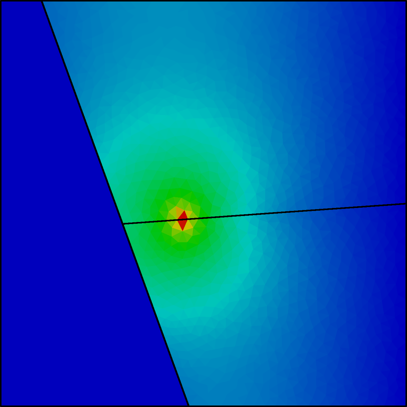
Figure 3: On the left, graphical example of problem (1.1)-(1.3) along with (4.2) in case of intersecting fractures. On the right, example of construction of a multiscale flux basis.

We impose the Darcy model (1.1) in each sub-domain $\Omega_{i}$ and the Darcy-Forchheimer model (1.2) in each fracture $\gamma_{i,j}$, with unknowns denoted by $({\mathbf{u}}_{\gamma_{i,j}},p_{\gamma_{i,j}})$. See Figure 3 (left) as an example.

They are coupled using the Robin boundary conditions given by

$$-{\mathbf{u}}_{i}\cdot{\mathbf{n}}_{i}+\alpha_{i,j}p_{i}=\alpha_{i,j}p_{\gamma_{i,j}}\quad\textnormal{on}\;\gamma_{i,j},$$ (4.1)

for $1\leq i<j\leq 3$, where the coefficient $\alpha_{i,j}$ can now be different in each fracture. To close the system, we need to impose transmission conditions between the fractures at the $(d-2)$-dimensional interface $T$. On the intersection $T$, we set

$$-{\mathbf{u}}_{\gamma_{i,j}}\cdot{\mathbf{n}}_{{i,j}}+\alpha_{\gamma_{i,j}}p_{\gamma_{i,j}}=\alpha_{\gamma_{i,j}}p_{T}\quad \textnormal{on}\;T,$$ (4.2a)

$$\sum_{1\leq i<j\leq 3}{\mathbf{u}}_{\gamma_{i,j}}\cdot{\mathbf{n}}_{i,j}=0\quad \textnormal{on}\;T,$$ (4.2b)

for $1\leq i<j\leq 3$ where ${\mathbf{n}}_{i,j}$ is the outer unit normal vector to $\partial\gamma_{i,j}.$

For the partition of the sub-domain $\Omega_{i}$, $1\leq i\leq 3$, and the fractures $\gamma_{i,j}$, $1\leq i<j\leq 3$, we extend the notation introduced in Subsection 2.1. We let $\mathcal{T}_{h,i}$ be a partition of the sub-domain $\Omega_{i}$ into $2$-dimensional simplicial elements and let $\mathcal{T}_{h,\gamma_{i,j}}$ to be a partition of the fracture $\gamma_{i,j}$ into $1$-dimensional simplicial elements. Again, the meshes $\mathcal{T}_{h,i}$, $1\leq i\leq 3$, are allowed to be non-conforming on the fractures $\gamma_{i,j}$, $1\leq i<j\leq 3$, but also different from those used in $\gamma_{i,j}$, $1\leq i<j\leq 3$ (see Figure 2 for more details). We also extend the same notation for the approximation spaces in the sub-domains and in the fractures, and additionally we let $M_{h,T}$ be the space endowed with constant functions on $T$.

4.2.2 Domain decomposition formulation

The extension of the reduced interface problem (2.5) to the present intersecting fractures setting is as follows: find the triplet $({\mathbf{u}}_{h,\gamma},p_{h,\gamma},p_{h,T})\in\mathbf{V}_{h,\gamma}\times M_{h,\gamma}\times M_{h,T}$ such that, for each $1\leq i<j\leq 3$,

$$\langle{\mathbf{\mathcal{K}}}^{-1}({\mathbf{u}}_{h,\gamma}){\mathbf{u}}_{h,\gamma},{\mathbf{v}}_{\gamma}\rangle_{\gamma_{i,j}}+\alpha_{\gamma_{i,j}}^{-1}\langle{\mathbf{u}}_{h,\gamma}\cdot{\mathbf{n}}_{i,j},{\mathbf{v}}_{\gamma}\cdot{\mathbf{n}}_{i,j}\rangle_{T}-\langle p_{h,\gamma},\nabla_{\tau}\cdot{\mathbf{v}}_{\gamma}\rangle_{\gamma_{i,j}}$$

$$\qquad\qquad\qquad\qquad\qquad\qquad\qquad\qquad\,\,\,\,=-\langle p_{h,T},{\mathbf{u}}_{\gamma_{i,j}}\cdot{\mathbf{n}}_{i,j}\rangle_{T}\quad \forall{\mathbf{v}}_{\gamma}\in\mathbf{V}_{h,\gamma_{i,j}},$$ (4.3a)

$$\langle\nabla_{\tau}\cdot{\mathbf{u}}_{h,\gamma},q_{\gamma}\rangle_{\gamma_{i,j}}+\langle\mathcal{S}_{\gamma_{i,j}}(p_{h,\gamma}),q_{\gamma}\rangle_{\gamma_{i,j}}=\langle f_{\gamma_{i,j}}+g_{\gamma_{i,j}},q_{\gamma}\rangle_{\gamma_{i,j}}\quad \forall q_{\gamma}\in M_{h,\gamma_{i,j}},$$ (4.3b)

$$\sum_{1\leq i<j\leq 3}\langle{\mathbf{u}}_{\gamma_{i,j}}\cdot{\mathbf{n}}_{i,j},q_{T}\rangle_{T}=0\quad \forall q_{T}\in M_{h,T}.$$ (4.3c)

On each fracture, the Robin-to-Neumann operator $\mathcal{S}_{\gamma_{i,j}}$ and the linear functional $g_{\gamma_{i,j}}$, $1\leq i<j\leq 3$, are now given by

$$\mathcal{S}_{\gamma_{i,j}}(p_{h,\gamma})\vcentcolon=\sum_{l\in(i,j)}\mathcal{S}^{\textnormal{RtN}}_{\gamma_{l}}(p_{h,\gamma},0)=-\sum_{l\in(i,j)}{\mathbf{u}}_{l}(p_{\gamma},0)\cdot{\mathbf{n}}_{l}|_{\gamma_{l}},$$

$$g_{\gamma_{i,j}}\vcentcolon=\sum_{l\in(i,j)}\mathcal{S}^{\textnormal{RtN}}_{\gamma_{l}}(0,f_{l})=\sum_{l\in(i,j)}{\mathbf{u}}_{l}(0,f_{l})\cdot{\mathbf{n}}_{l}|_{\gamma_{i}}.$$

The above problem can be seen as a DFNs system on the set of fractures, and as a domain decomposition problem between the $1$-dimensional fractures $\gamma_{i,j}$, $1\leq i<j\leq 3$, cf.[38, 39, 20] for more details.

4.2.3 Iterative procedure

We propose to solve the non-linear domain decomposition problem (4.3) using the fixed-point approach in Subsection 3.1. This iterative process is now equipped with the multiscale flux basis of Section 4 to lessen the interface iterations. To this aim, we introduce

$$\mathcal{S}_{\gamma}(p_{h,\gamma})\vcentcolon=\sum_{0\leq i<j\leq 3}\mathcal{S}_{\gamma_{i,j}}(p_{h,\gamma})\quad\text{and}\quad g_{\gamma}\vcentcolon=\sum_{1\leq i<j\leq 3}g_{\gamma_{i,j}},$$

and let

$$\mathcal{S}_{T}(p_{h,T})\vcentcolon=\sum_{1\leq i<j\leq 3}{\mathbf{u}}_{\gamma_{i,j}}\cdot{\mathbf{n}}_{i,j}|_{T}.$$

Applying the fixed-point algorithm on the set of interface Darcy-Forchheimer equations (4.3) can be interpreted as follows: at the iteration $k\geq 1$, we solve

$$\begin{bmatrix}{\mathbf{\mathcal{K}}}^{-1,(k)}_{\gamma}&B_{\gamma}^{\textnormal{T}}&\mathcal{S}^{\textnormal{T}}_{T}\\[5.69054pt] B_{\gamma}&\mathcal{S}_{\gamma}&0\\[5.69054pt] \mathcal{S}_{T}&0&0\\[5.69054pt] \end{bmatrix}\begin{bmatrix}{\mathbf{u}}^{k}_{h,\gamma}\\[5.69054pt] p^{k}_{h,\gamma}\\[5.69054pt] p^{k}_{h,T}\end{bmatrix}=\begin{bmatrix}0\\[5.69054pt] f_{\gamma}+g_{\gamma}\\[5.69054pt] 0\end{bmatrix},$$ (4.5)

using GMRes method until a fixed tolerance is reached. Again, the evaluation of $\mathcal{S}_{\gamma}$ in each interface GMRes iteration dominates the total computational costs of this outer–inner procedure. Note that each inner iteration also requires the evaluation of the Dirichlet-to-Neumann operator $\mathcal{S}_{T}$, which requires solves in the fractures. The complete algorithm when equipped with multiscale flux basis is now given by the following algorithm.

Algorithm 4.3 (Fixed-point algorithm with multiscale flux basis for fracture network model).

1. Enter the source terms and the permeabilities in the fractures and the rock matrices.

2. Choose the meshes $\mathcal{T}_{h,i}$, $1\leq i\leq 3$, and $\mathcal{T}_{h,\gamma_{i,j}}$, $1\leq i<j\leq 3$.

3. Calculate the right-hand-sides $g_{\gamma_{i,j}}$, $1\leq i<j\leq 3$, by solving the Darcy sub-domain problem in $\Omega_{i}$ with source term $f_{i}$ and zero Robin value on the fracture-interface $\gamma_{i}$. Then, compute the resulting jump across all sub-domain interfaces.

4. In the sub-domain $\Omega_{i}$, $1\leq i\leq 3$, let $\mathcal{N}_{h,\gamma_{i}}$ be the number of degrees of freedom in the space $M_{h,\gamma_{i}}$. Define the basis $(\Phi^{\ell}_{h,\gamma_{i}})^{\mathcal{N}_{h,\gamma_{i}}}_{\ell=1}$. Set $i=0$.
   Do {Assembly of the multiscale flux basis}

   1. Increase $i\vcentcolon=i+1$.

   2. Compute the multiscale flux basis functions $(\Psi^{\ell}_{h,\gamma_{i}})^{\mathcal{N}_{h,\gamma_{i}}}_{\ell=1}$ corresponding to $(\Phi^{\ell}_{h,\gamma_{i}})^{\mathcal{N}_{h,\gamma_{i}}}_{\ell=1}$ using Algorithm 4.3, i.e.,

      $$\Psi^{\ell}_{h,\gamma_{i}}\vcentcolon=\mathcal{S}^{\textnormal{RtN}}_{\gamma_{l}}(\Phi^{\ell}_{h,\gamma_{i}},0),\quad\ell=1,\cdots,\mathcal{N}_{h,\gamma_{i}}.$$

   While $i\leq 3$.

5. Given an initial guess ${\mathbf{u}}^{(0)}_{h,\gamma_{i,j}}$, $1\leq i<j\leq 3$. Set $k=0$.
   Do {Fixed-point iterations}

   1. Increase $k\vcentcolon=k+1$.

   2. Solve the linear system on the fractures (4.5) using GMRes method (2.8), where in every iteration the operator action $\mathcal{S}_{\gamma}$ on any $\varphi_{h,\gamma}\in M_{h,\gamma}$ is computed with the following steps:

      1. Use a linear combination of the multiscale flux basis to compute the action of $\mathcal{S}^{\textnormal{RtN}}_{\gamma_{i}}$ by

         $$\mathcal{S}^{\textnormal{RtN}}_{\gamma_{i}}(\varphi_{h,\gamma,i},0)\vcentcolon=\sum_{\ell=1}^{\mathcal{N}_{h,\gamma,i}}\varphi^{\ell}_{h,\gamma,i}\Psi^{\ell}_{h,\gamma,i}.$$

      2. Compute the jump across all the fractures:

         $$\mathcal{S}_{\gamma}(\varphi_{h,\gamma})\vcentcolon=\sum_{0\leq i<j\leq 3}\sum_{l\in(i,j)}\mathcal{S}^{\textnormal{RtN}}_{\gamma_{l}}(\varphi_{h,\gamma},0).$$

   While $\dfrac{\|(p^{k,\infty}_{h,\gamma},{\mathbf{u}}^{k,\infty}_{h,\gamma})-(p^{k-1,\infty}_{h,\gamma},{\mathbf{u}}^{k-1,\infty}_{h,\gamma})\|_{\infty}}{\|(p^{k-1,\infty}_{h,\gamma},{\mathbf{u}}^{k-1,\infty}_{h,\gamma})\|_{\infty}}\geq\varepsilon_{tol}$. 4.6

5 Numerical examples

In this section, we validate the model and analysis presented in the previous parts by means of numerical test cases. We have chosen three examples designed to show how the proposed linearization–domain-decomposition approaches equipped with multiscale flux basis behaves vs the standard ones in various physical and geometrical situations. To compare these approaches, the main criteria considers the number of solutions of the higher-dimensional sub-problems since it constitutes the major computational cost. We consider solving the problem in the network of fractures as negligible. Since each of the higher-dimensional sub-problem is linear and will be solved many times, we consider an LU-factorization of the system matrix and a forward-backward substitution algorithm to compute the numerical solution. It results in a computational cost reduced to $\mathcal{O}(n^{2})$ flops each time, where $n$ is the size of the matrix. For bigger systems, an iterative scheme is preferable.

We use the PorePy [27] library, which is a simulation tool for fractured and deformable porous media written in Python. PorePy uses SciPy [26] as default sparse linear algebra. All the examples are reported in the GitHub repository of PorePy, we want to stress again that even if we focus on lowest-order Raviart-Thomas-Nédélec finite elements, our implementation is agnostic with respect to the numerical scheme.

For the multiscale flux basis scheme presented in Section 4, for a fixed rock matrix grid and normal fracture permeability it is possible to compute once all the basis functions. The results in the next parts should be read under this important property of the method, thus in many cases only a pure fracture network will be solved at a negligible computational cost. The multiscale basis functions are computed and stored in an offline phase prior the simulation (called online).

Unless otherwise noted, the tolerance for the relative residual in the inner GMRes algorithm is taken to be $10^{-6}$. The same tolerance is chosen for the outer Newton/fixed-point algorithm. We consider an LU-factorization of the fracture network matrix [8, 11] as the preconditioner of the GMRes method.

In the examples, we use the abbreviation MS when the linearization–domain–decomposition approach is equipped with multiscale flux basis techniques, and DD for the corresponding classical approach.

Remark 5.1 (Fracture aperture).

Even if not explicitly considered in the previous parts of the work, we introduce the fracture aperture $\epsilon$ as a constant parameter. This choice is based on the fact that geometries and (some) data of the forthcoming examples are taken from the literature.

In 5.1 we describe the geometry and some data of the problem considered. Few subsections follows with an increase level of challenge: linear case in 5.2, Forchheimer model in 5.3, Forchheimer model with heterogeneous parameters in 5.4, to conclude with a generalized Forchheimer model in 5.5.

5.1 Problem setting

To validate the performance of the two proposed algorithms, we consider the first problem presented in the benchmark study [15]. The unit square domain $\Omega$, depicted in Figure 4, has unitary permeability of the rock matrix and it is divided into 10 sub-domains by a set of fractures with fixed aperture $\epsilon$ equal to $10^{-4}$.

Figure 4: Graphical representation of the domain and fracture network geometry common for all test cases.

At the boundary, we impose zero flux condition on the top and bottom, unitary pressure on the right, and flux equal to $-1$ on the left. The boundary conditions are applied to both the rock matrix and the fracture network.

Contrary to what has been done in the benchmark paper, we consider four different scenarios for the fracture permeabilities, by having high or low values in the tangential and normal parts. Thus, we have the case (i) with high permeable fractures, case (ii) has low permeable fractures, while cases (iii) and (iv) have mixed high and low permeability in normal and tangential directions. See Table 1 for a summary of the fracture permeability in each case.

	$\mathbf{K}_{\gamma}$	$\alpha_{\gamma}$
case (i)	$10^{4}\epsilon\mathbf{I}$	$10^{4}/\epsilon$
case (ii)	$10^{-4}\epsilon\mathbf{I}$	$10^{-4}/\epsilon$
case (iii)	$10^{4}\epsilon\mathbf{I}$	$10^{-4}/\epsilon$
case (iv)	$10^{-4}\epsilon\mathbf{I}$	$10^{4}/\epsilon$

Table 1: Definition of the cases for the examples.

Case (i) and (ii) have the same permeabilities used in the benchmark paper [15].

In the following examples, we consider the maximal number of rock matrix solves to be $10^{4}$, and we mark with $\infty$ if this is exceeded.

5.2 Darcy model: $\beta_{\gamma}=0$

The first example considers the Forchheimer coefficient set to zero, thus the problem becoming linear. The results for different level of discretization are reported in Table 2. We indicate by level 1 a grid with 110 triangles and 26 segments, level 2 with 1544 triangles and 84 segments, and level 3 with 3906 triangles and 138 segments.

	level 1		level 2		level 3
	MS	DD	MS	DD	MS	DD
case (i)	28†	10	86†	11	140†	11
case (ii)	28§	81	86§	112	140§	189
case (iii)	28§	22	86§	28	140§	29
case (iv)	28†	82	86†	61	140†	86

Table 2: Total number of the higher-dimensional problem solves for the case study of example in Subsection 5.2. For each level of refinement cases marked in $\dagger$ share the same multiscale flux basis, which can be constructed only once. The same is valid for ${\mathsection}$.

Table 2 shows the results of this example for the physical considerations of Table 1. We notice that for high permeable fractures (case (i) and (iii)), the standard domain decomposition method performs better than our method with multiscale flux basis, while the opposite occurs for low permeable fractures. A possible explanation is related to the ratio between normal and tangential permeability. The normal permeability determines how strong the flux exchange is between the rock matrix and the fractures (thus, the communications at each DD iteration), while for small values of the tangential permeability the fractures are more influenced by the surrounding rock matrices. The opposite occurs in the case of high tangential permeability. Additionally, the choice of the preconditioner for DD slightly goes in favor of high permeable fractures due to the dominating role of the fracture flow in the system. We also recall that the number of higher-dimensional problem solves does not depend on the number of outer–inner interface iterations, but only on the number of local mortar degrees of freedom on the fractures network. A further important result in this experiments, is that case (i) and (iv) share the same value of $\alpha_{\gamma}$, thus the multiscale flux basis are computed only once per level of refinement. The same applies to case (ii) and (iii). As a result, the developed method is globally more efficient than the classical approach. That is, the results in Table 2 shows a reduction of the number of the higher-dimensional problem solves from 195 to 56 for level 1, from 212 to 186 for level 2, and from 312 to 280 for level 3. Note that the two methods produce the same solution for all the cases, within the same relative convergence tolerance. The numerical solution for all cases is reported in Figure 5.

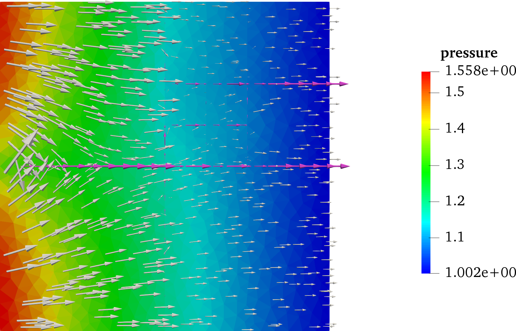
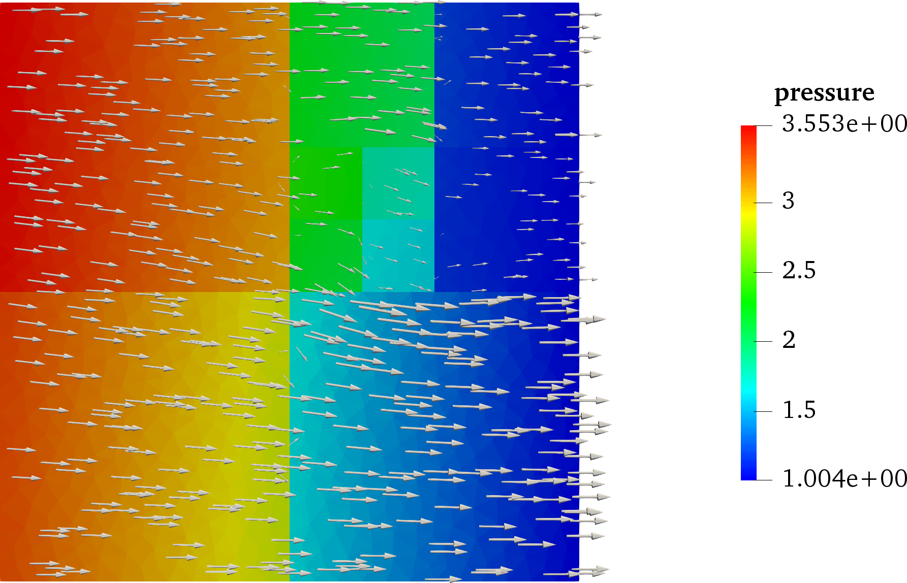
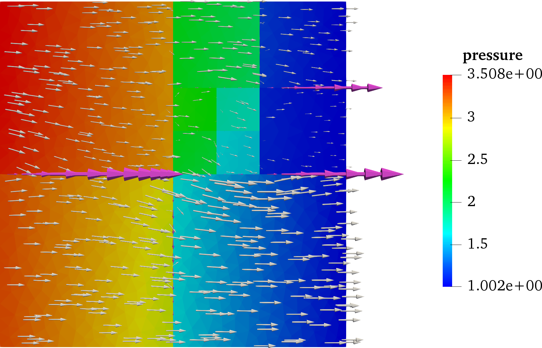
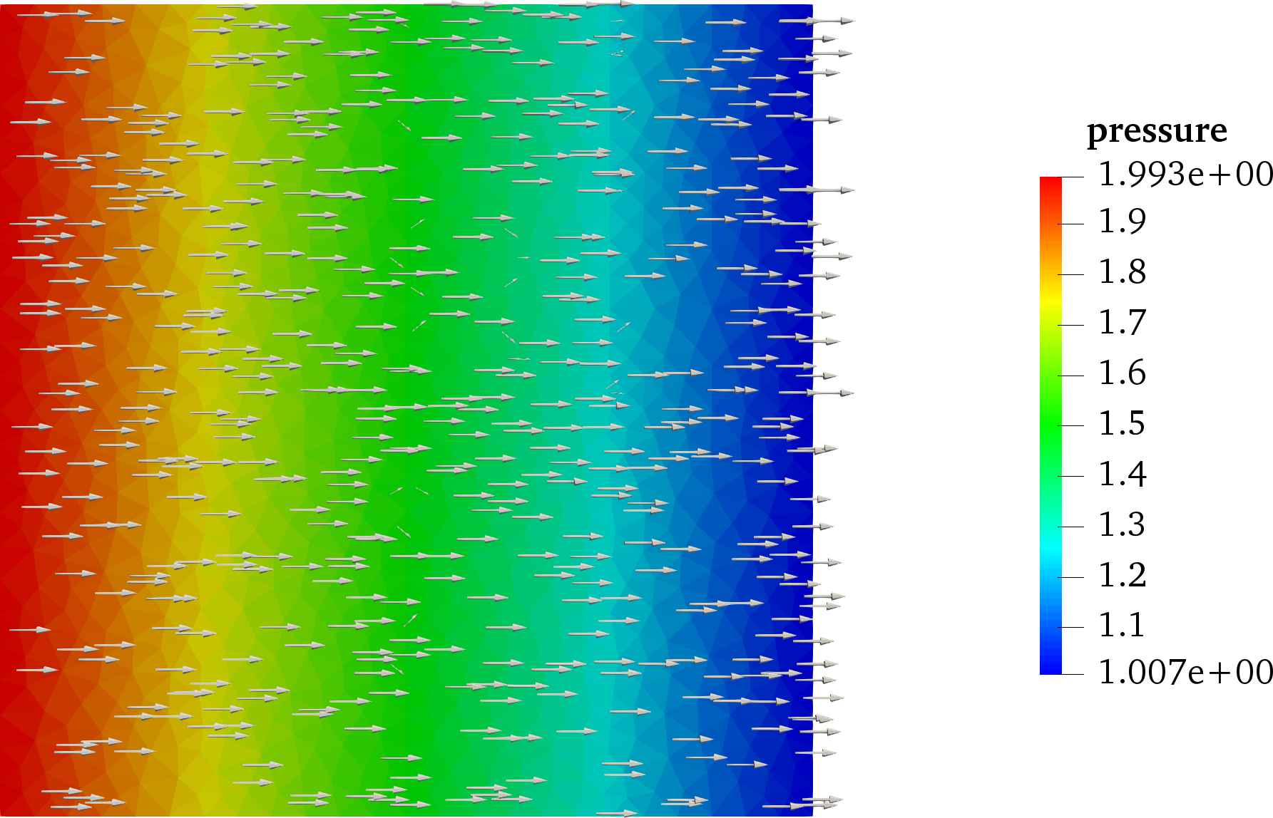
Figure 5: Pressure and velocity solutions for the four cases: on the top-left case (i), on the top-right case (ii), on the bottom-left case (iii), and on the bottom-right case (iv). In all the cases, the velocity is represented by arrows (purple for the fractures) proportional to its magnitude.

The next series of numerical experiments aims at assessing the stability of the domain decomposition approach with respect to GMRes tolerance. The multiscale flux basis approach provides the extra flexibility to do such analysis with negligible costs, by reusing the stored multiscale flux basis used for the results of Table 2 but now with different tolerance for GMRes. Further, this set of test cases aims assessing how the overall gain for an entire simulation in terms of number of higher-dimensional problem solves can be appreciated or depreciated with more or less stringent stopping criteria for GMRes; this is a preparatory step to address the complete approaches of Section 3 for the full nonlinear problem, which requires several solves of linear Darcy problems, for which one should formulate the stopping criteria very carefully. In Table 2, we have considered the relative residual to be below $10^{-6}$, while in Table 3 we present the results in the case of $10^{-4}$ and $10^{-8}$. Based on the results of Table 3, we can conclude that even with less stringent criterion, a considerable gain in terms of number of higher-dimensional problem solves can be achieved. We also see that all the results are free of oscillations and neither the fracture, barrier, or the very different tangential and normal permeabilities pose any problems for the domain decomposition approach. Based on the above results and in what follows we consider $10^{-6}$ as tolerance for the GMRes algorithm.

	level 1		level 2		level 3
tolerance	$10^{-4}$	$10^{-8}$	$10^{-4}$	$10^{-8}$	$10^{-4}$	$10^{-8}$
case (i)	8	11	9	12	9	12
case (ii)	42	105	82	$\infty$	150	$\infty$
case (iii)	21	30	22	36	22	36
case (iv)	42	122	50	$\infty$	70	$\infty$

Table 3: Total number of the higher-dimensional problem solves for the case study of example in Subsection 5.2. For each level of refinement we change the convergence tolerance for the domain decomposition method.

5.3 Forchheimer model

In this second example we consider case (i) and (iii) for the fracture permeabilities since the Forchheimer model requires high permeable fractures. In this problem, we fix the computational grid level 2 of Table 2 and we change the value of $\beta_{\gamma}$ in order to compare the performances of Method 1 and Method 2 with and without multiscale flux basis. The Forchheimer coefficient here varies as $\{1,10^{2},10^{4},10^{6}\}$. These values are reasonable since in our model we do not explicitly scale $\beta_{\gamma}$ by the aperture, as done in [19, 29]. Therefore, the last two values are more realistic. The stopping criteria for both methods is based on the relative residual criteria (5) with a threshold fixed as $10^{-6}$. The initial guess is taken by solving the linear Darcy by taking $\beta_{\gamma}$ equal to zero.

	case (i)		case (iii)
$\beta_{\gamma}$	MS	DD	MS	DD
$1$	86† (2)	33 (2)	86§ (1)	56 (1)
$10^{2}$	86† (3)	44 (3)	86§ (2)	84 (2)
$10^{4}$	86† (8)	99 (8)	86§ (3)	115 (3)
$10^{6}$	86† (94)	1424 (94)	86§ (11)	457 (11)

Table 4: Total number of the higher-dimensional problem solves required by Method 1 for the case study in Subsection 5.3. The number of the fixed-point iterations are in brackets. Within each case the construction of the multiscale flux basis is done only once, we mark by $\dagger$ (respectively ${\mathsection}$) common computations.

For Method 1, the number of higher-dimensional problem solves is reported in Table 4. As expected, Method 1 equipped with multiscale flux basis (MS) performs all the higher-dimensional problem solves in the offline phase, thus the outer–inner interface iterations for the resulting fracture network problem do not influence the total computational costs. On the contrary, the computational costs of the classical approach (DD) is influenced by the non-linearity, by varying $\beta_{\gamma}$, as well as by the ratio of the normal and tangential permeabilities, by varying $\mathbf{K}_{\gamma}$ and $\alpha_{\gamma}$. Particularly, the total gain of the new approach is more significant when the non-linear effects becomes more important (by increasing the value of $\beta_{\gamma}$). Furthermore, for the entire simulation of each case of Table 4, the multiscale flux basis are computed only once. As a conclusion, the entire simulation of case (i) required for Method 1 1600 higher-dimensional problem solves, while for Method 1 with multiscale flux basis, this number is reduced by $95\%$. For case (iii), we reduce the computational costs by $88\%$.

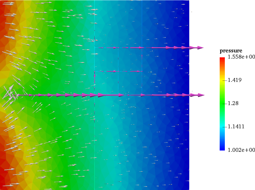
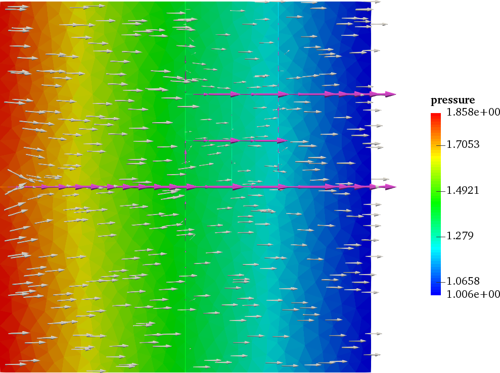
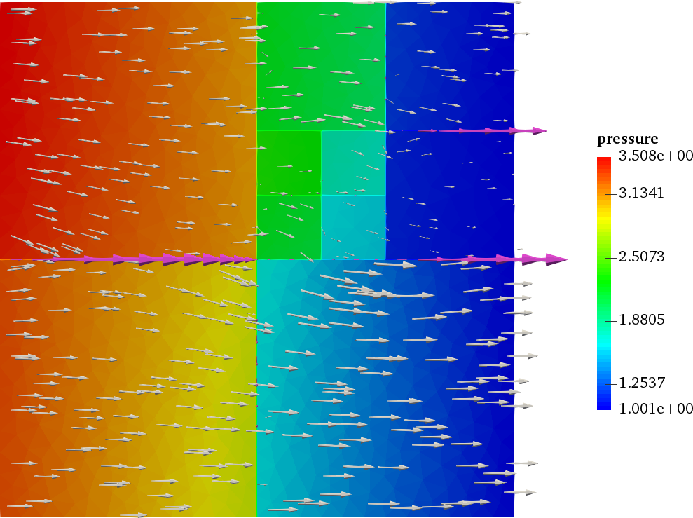
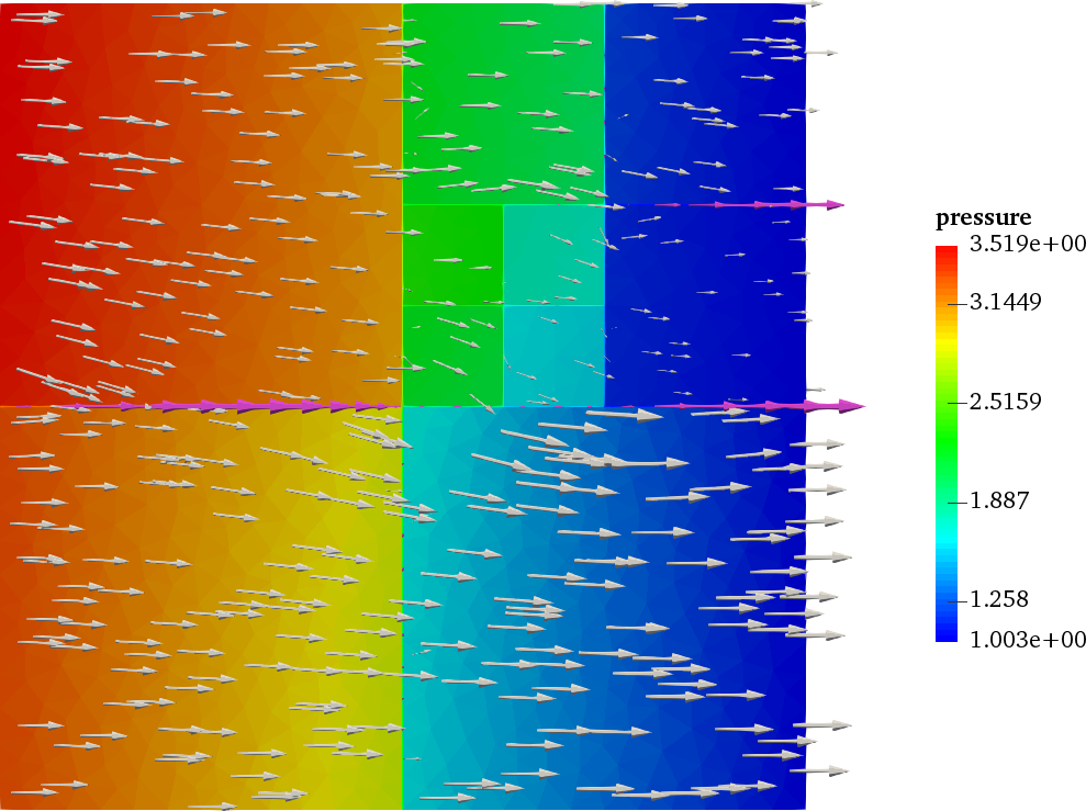
Figure 6: Pressure and velocity solutions for different configurations of example presented in Subsection 5.3. On the top case (i) and on the bottom for case (iii). On the left, we consider value of the Forchheimer coefficient equal to $\beta_{\gamma}=1$ and on the right a high value $\beta_{\gamma}=10^{6}$. In all the cases, the velocity is represented by arrows (purple for the fractures) proportional to its magnitude.

The numerical solution for two values of $\beta_{\gamma}$ are reported in Figure 6 for both cases. Despite the different values of $\beta_{\gamma}$, we notice that the graphical results are very similar in the case of low $\alpha_{\gamma}$. While for high value of $\alpha_{\gamma}$, the resulting apparent permeability given by $\mathbf{K}_{\gamma}(1+\mathbf{K}_{\gamma}^{-1}\beta_{\gamma}|\mathbf{u}_{\gamma}|)^{-1}$ decreases (for a fixed $|\mathbf{u}_{\gamma}|$) and the fractures are less prone to be the main path for the flow. Also as stated previously, since we do not explicitly scale $\beta_{\gamma}$ by the aperture, values of $\beta_{\gamma}>10^{4}$ are more likely for real applications.

	case (i)		case (iii)
$\beta_{\gamma}$	MS	DD	MS	DD
$1$	86† (2)	20 (2)	86§ (1)	38 (1)
$10^{2}$	86† (2)	20 (2)	86§ (2)	71 (2)
$10^{4}$	86† (3)	31 (3)	86§ (2)	71 (2)
$10^{6}$	86† (7)	128 (7)	86§ (4)	266 (6)

Table 5: Total number of the higher-dimensional problem solves required by Method 2 for the case study in Subsection 5.3. The number of the Newton iterations are in brackets. Within each case the construction of the multiscale flux basis is done only once, we mark by $\dagger$ (respectively ${\mathsection}$) common computations.

For Method 2, involving Newton’s method for the linearization step, the number of higher-dimensional problem solves are reported in Table 5. As expected, Method 2 is more efficient than Method 1 in terms of the number of higher-dimensional problem solves required, regardless of using multiscale flux basis in the domain decomposition algorithm. Again, the number of solves for the classical approach(DD) depends on the used parameters. This table demonstrates (as shown with Method 1) that as the value of $\beta_{\gamma}$ is increased, there is a point after which Method 2 with multiscale flux basis is more efficient than without multiscale flux basis. In that case, the gain in the number of solves becomes more significant when decreasing the value of $\alpha_{\gamma}$. Note that, in practice, the simulations for Method 2 with multiscale flux basis are performed with negligible computational costs as we reused the flux basis inherited from Method 1. This point together with the fact that the total number of solves required by the entire simulation of case (i) is now reduced by $57\%$ as well as that of case (i) is reduced by $80\%$ showcase the performance of Method 2 with multiscale flux basis.

To sum up, equipping Method 1 and 2 with multiscale flux basis leads to powerful tools to solve complex fracture network with important savings in terms of the number of higher-dimensional problem solves. Note that, as known, one limitation of Method 2 involving Newton method is that a good initial value is usually required to obtain a solution. A good combination of both methods can also be used, in which one can perform first some fixed-point iterations and then switch to Newton method. Concerning the computational costs, let us point out that the fixed-point algorithm of Method 1 requires at each iteration the assembly of the matrix corresponding to the linearization of the Darcy-Forchheimer equations and the solution of a linear system. The Newton method in Method 2 is slightly more expensive since one has to assemble two matrices at each iteration and to update the right-hand side.

5.4 Heterogeneous Forchheimer model

In this example we assign to the two biggest fractures (one horizontal and one vertical) high permeability while to the others low permeability. For the highly permeable fractures we adopt the physical parameters of case (i), while for those with lower permeabilities, the physical parameters corresponding to case (ii) together with zero Forchheimer coefficient. In this case, we want to test the applicability of Method 1 with and without multiscale flux basis on highly heterogeneous setting for both the permeability and the flow models. We consider level 2 for the computation and, subsequently, the local grids of the low permeable fractures are coarsened by having half of the original number of elements resulting in 60 mortar unknowns instead of 84.

As usually, we compare the method with and without multiscale flux basis in terms of the number of higher-dimensional problem solves. The results are represented in Table 6.

$\beta_{\gamma}$	MS	DD
$1$	62† (2)	63 (2)
$10^{2}$	62† (3)	84 (3)
$10^{4}$	62† (8)	189 (8)
$10^{6}$	62† (64)	2372 (64)

Table 6: Total number of the higher-dimensional problem solves required by Method 1 for the case study in Subsection 5.4. The number of the fixed-point iterations are in brackets. Within each case the construction of the multiscale basis is done only once, we mark by $\dagger$ common computations.

In the present setting, we can see that the classical approach is outperformed with the approach equipped with multiscale flux basis, particularly, the total computational costs is drastically reduced when the non-linear effects becomes more important. The entire simulation of Table 6 required 2708 higher-dimensional problem solves for the classical approach while the same approach equipped with multiscale flux basis required 62 solves. The overall gain is then of $94\%$ which can also be appreciated for level 3. Similar conclusions as above can be drawn for Method 2, namely in terms of reduction of the solves (not shown). An example of solution is given in Figure 7.

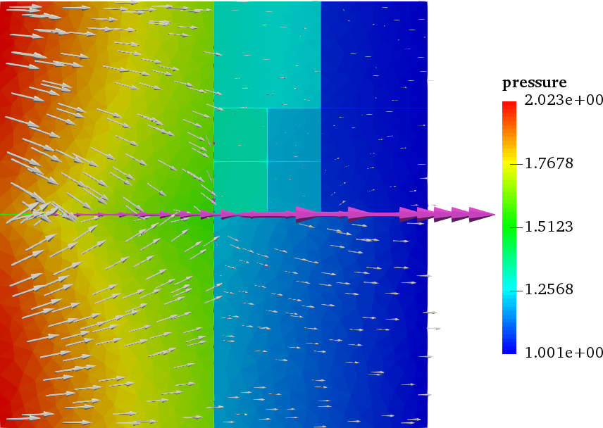
Figure 7: Pressure and velocity solutions for example presented in Subsection 5.4 for $\beta=10^{2}$. The velocity is represented by arrows (purple for the fractures) proportional to its magnitude.

5.5 Generalized Forchheimer model

As stated previously, another advantage distinguishes our approach is that it can integrate easily more complex problems. Here, we apply our procedure to a more general model describing the pressure-flow relation in the fractures. Precisely, for larger fracture flow velocities, the drag forces (in the Forchheimer model proportional to the velocity norm) require to consider an additional term proportional to the fluid viscosity. Considering the Barus formula [7], we have an exponential relation between the fluid viscosity and the pressure. We consider problem (2.1) where the non-linear term is as follows

$${\mathbf{\mathcal{K}}}^{-1}({\mathbf{u}}_{\gamma},p_{\gamma})=\mathbf{K}^{-1}_{\gamma}e^{\zeta p_{\gamma}}+\beta_{\gamma}{\textbf{I}}|{\mathbf{u}}_{\gamma}|,$$

where $\zeta$ being a model parameter. Thus, the non-linear effects are now dependent on both the pressure and the velocity. For a more detailed discussion we refer to [40]. For the present setting, the fracture permeabilities are set as in case (i) and (iii) of Table 1.

For the discretization of the mixed geometry, we consider level 2. We use Method 1 with and without multiscale basis functions. Also, it was not necessary to recompute the basis functions, since we can reuse the stored multiscale flux basis from the previous test case and solve then only on the fracture network the above more complex Darcy-Forchheimer model. The total number the higher-dimensional problem solves for $\beta_{\gamma}=20$ and $\zeta\in(0.5,5,7.5)$ is reported in Table 7.

	case (i)		case (iii)
$\zeta$	MS	DD	MS	DD
$0.5$	86† (5)	71 (5)	86§ (4)	176 (4)
$5$	86† (4)	648 (4)	86§ (6)	$\infty$
$7.5$	86† (3)	5317 (3)	86§ (4)	$\infty$

Table 7: Total number of the higher-dimensional problem solves required by Method 1 for the case study in Subsection 5.5. The number of the fixed-point iterations are in brackets. Within each case the construction of the multiscale basis is done only once, we mark by $\dagger$ (respectively ${\mathsection}$) common computations.

As expected, for such a strong non-linearity, the results shows that a considerable gain in terms of higher-dimensional problem solves can be achieved. Particularly, for large values of $\zeta$ the classical approach becomes uncompetitive to the new approach.

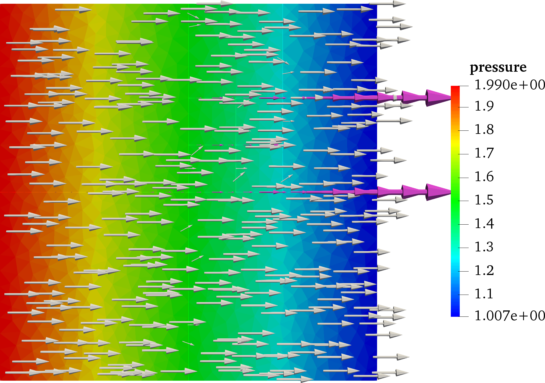
Figure 8: Pressure and velocity solutions for example presented in Subsection 5.5 for $\zeta=5$. The velocity is represented by arrows (purple for the fractures) proportional to its magnitude.

In Figure 8 we report the solution for $\zeta=5$.

6 Conclusions

In this work, we have presented a strategy to speed up the computation of a Darcy-Forchheimer model for flow and pressure in fractured porous media by means of multiscale flux basis, that represent the inter-dimensional flux exchange. The scheme transforms a computationally expensive discrete fracture model to a more affordable discrete fracture network, where in the latter only a co-dimensional problem is solved. The multiscale flux basis are computed in an offline stage of the simulation and, despite the particular choice done in this paper, are completely agnostic to the model in the fracture network. The numerical results show the speed-up gain compared to a more classical linearization–domain-decomposition approaches, where solves in both the matrix and the fracture network are required along the entire outer–inner iterative method. Crucially, an important number of the outer–inner interface iterations may be spared.

With the proposed approach we are able to predict the computational effort needed to solve the problem since it is directly related to the number of mortar grids in the fracture network. Furthermore, the multiscale flux basis can be reused when the fracture network geometry, rock matrix properties, and normal permeability are fixed. Theoretical findings and numerical results show the validity of the proposed approach and of its aforementioned properties.

Even if not explicitly considered in this work, it is possible to further increase the efficiency of the proposed scheme by the following two steps. First, compute a multiscale flux basis only in the related connected part of the rock matrix. Second, use an adaptive stopping criteria for the inner–outer iterative method based on a posteriori error estimates. These enhancements are a part of future work along with the extension in three-dimensions.

References

- [1] E. Ahmed, J. Jaffré, and J. E. Roberts, A reduced fracture model for two-phase flow with different rock types, Math. Comput. Simulation, 137 (2017), pp. 49–70, https://doi.org/10.1016/j.matcom.2016.10.005, https://doi.org/10.1016/j.matcom.2016.10.005.
- [2] C. Alboin, J. Roberts, and C. Serres, Domain Decomposition for Flow in Porous Media With Fractures, (1999).
- [3] L. Amir, M. Kern, V. Martin, and J. E. Roberts, D composition de domaine et pr conditionnement pour un mod le 3D en milieu poreux fractur , in Proceeding of JANO 8, 8th conference on Numerical Analysis and Optimization, Dec. 2005. 2005.
- [4] L. Amir, M. Kern, J. E. Roberts, and V. Martin, Décomposition de domaine pour un milieu poreux fracturé: un modèle en 3D avec fractures, Revue Africaine de la Recherche en Informatique et Mathématiques Appliquées, 5 (2006), pp. 11–25.
- [5] P. Angot, F. Boyer, and F. Hubert, Asymptotic and numerical modelling of flows in fractured porous media, M2AN Math. Model. Numer. Anal., 43 (2009), pp. 239–275, https://doi.org/10.1051/m2an/2008052, https://doi.org/10.1051/m2an/2008052.
- [6] P. F. Antonietti, L. Formaggia, A. Scotti, M. Verani, and N. Verzott, Mimetic finite difference approximation of flows in fractured porous media, ESAIM Math. Model. Numer. Anal., 50 (2016), pp. 809–832, https://doi.org/10.1051/m2an/2015087, https://doi.org/10.1051/m2an/2015087.
- [7] C. Barus, Isothermals, isopiestics and isometrics relative to viscosity, American Journal of Science, 45 (1893), pp. 87–96.
- [8] M. Benzi, Preconditioning techniques for large linear systems: a survey, J. Comput. Phys., 182 (2002), pp. 418–477, https://doi.org/10.1006/jcph.2002.7176, https://doi.org/10.1006/jcph.2002.7176.
- [9] C. D’Angelo and A. Scotti, A mixed finite element method for Darcy flow in fractured porous media with non-matching grids, ESAIM: Mathematical Modelling and Numerical Analysis, 46 (2012), pp. 465–489, https://doi.org/10.1051/m2an/2011148.
- [10] M. Del Pra, A. Fumagalli, and A. Scotti, Well posedness of fully coupled fracture/bulk Darcy flow with XFEM, SIAM J. Numer. Anal., 55 (2017), pp. 785–811, https://doi.org/10.1137/15M1022574, https://doi.org/10.1137/15M1022574.
- [11] J. W. Demmel, N. J. Higham, and R. S. Schreiber, Numer. Linear Algebra Appl., pp. 173–190, https://doi.org/10.1002/nla.1680020208.
- [12] Y. Efendiev and T. Y. Hou, Multiscale Finite Element Methods: Theory and Applications, Surveys and tutorials in the applied mathematical sciences, Springer-Verlag, 2009.
- [13] R. Eymard, T. Gallouët, and R. Herbin, mixed finite elements for some nonlinear problems, Math. Comput. Simulation, 118 (2015), pp. 186–197, https://doi.org/10.1016/j.matcom.2014.11.013, https://doi.org/10.1016/j.matcom.2014.11.013.
- [14] I. Faille, A. Fumagalli, J. Jaffré, and J. E. Roberts, Model reduction and discretization using hybrid finite volumes for flow in porous media containing faults, Comput. Geosci., 20 (2016), pp. 317–339, https://doi.org/10.1007/s10596-016-9558-3, https://doi.org/10.1007/s10596-016-9558-3.
- [15] B. Flemisch, I. Berre, W. Boon, A. Fumagalli, N. Schwenck, A. Scotti, I. Stefansson, and A. Tatomir, Benchmarks for single-phase flow in fractured porous media, Advances in Water Resources, 111 (2018), pp. 239–258, https://doi.org/10.1016/j.advwatres.2017.10.036, https://www.sciencedirect.com/science/article/pii/S0309170817300143.
- [16] L. Formaggia, A. Fumagalli, A. Scotti, and P. Ruffo, A reduced model for Darcy’s problem in networks of fractures, ESAIM Math. Model. Numer. Anal., 48 (2014), pp. 1089–1116, https://doi.org/10.1051/m2an/2013132, https://doi.org/10.1051/m2an/2013132.
- [17] N. Frih, V. Martin, J. E. Roberts, and A. Saâda, Modeling fractures as interfaces with nonmatching grids, Computational Geosciences, 16 (2012), pp. 1043–1060, https://doi.org/10.1007/s10596-012-9302-6, https://doi.org/10.1007/s10596-012-9302-6.
- [18] N. Frih, J. E. Roberts, and A. Saada, Modeling fractures as interfaces: a model for Forchheimer fractures, Comput. Geosci., 12 (2008), pp. 91–104, https://doi.org/10.1007/s10596-007-9062-x, https://doi.org/10.1007/s10596-007-9062-x.
- [19] N. Frih, J. E. Roberts, and A. Saada, Modeling fractures as interfaces: a model for Forchheimer fractures, Computers and Geosciences, 12 (2008), pp. 91–104, https://doi.org/10.1007/s10596-007-9062-x.
- [20] A. Fumagalli and E. Keilegavlen, Dual virtual element method for discrete fractures networks, SIAM J. Sci. Comput., 40 (2018), pp. B228–B258, https://doi.org/10.1137/16M1098231, https://doi.org/10.1137/16M1098231.
- [21] B. Ganis, G. Pencheva, M. F. Wheeler, T. Wildey, and I. Yotov, A frozen Jacobian multiscale mortar preconditioner for nonlinear interface operators, Multiscale Model. Simul., 10 (2012), pp. 853–873, https://doi.org/10.1137/110826643, https://doi.org/10.1137/110826643.
- [22] B. Ganis and I. Yotov, Implementation of a mortar mixed finite element method using a multiscale flux basis, Computer Methods in Applied Mechanics and Engineering, 198 (2009), pp. 3989–3998, https://doi.org/10.1016/j.cma.2009.09.009, http://www.sciencedirect.com/science/article/pii/S0045782509003077.
- [23] B. Ganis and I. Yotov, Implementation of a mortar mixed finite element method using a multiscale flux basis, Comput. Methods Appl. Mech. Engrg., 198 (2009), pp. 3989–3998, https://doi.org/10.1016/j.cma.2009.09.009, https://doi.org/10.1016/j.cma.2009.09.009.
- [24] H. Hægland, A. Assteerawatt, H. Dahle, G. Eigestad, and R. Helmig, Comparison of cell- and vertex-centered discretization methods for flow in a two-dimensional discrete-fracture–matrix system, Advances in Water Resources, 32 (2009), pp. 1740–1755, https://doi.org/10.1016/j.advwatres.2009.09.006, http://www.sciencedirect.com/science/article/pii/S030917080900150X.
- [25] T.-T.-P. Hoang, C. Japhet, M. Kern, and J. E. Roberts, Space-time domain decomposition for reduced fracture models in mixed formulation, SIAM J. Numer. Anal., 54 (2016), pp. 288–316, https://doi.org/10.1137/15M1009651, https://doi.org/10.1137/15M1009651.
- [26] E. Jones, T. Oliphant, P. Peterson, et al., SciPy: Open source scientific tools for Python, 2001–, http://www.scipy.org/. [Online].
- [27] E. Keilegavlen, A. Fumagalli, R. Berge, I. Stefansson, and I. Berre, Porepy: An open source simulation tool for flow and transport in deformable fractured rocks, tech. report, arXiv:1712.00460 [cs.CE], 2017, https://arxiv.org/abs/1712.00460.
- [28] P. Knabner and J. E. Roberts, Mathematical analysis of a discrete fracture model coupling Darcy flow in the matrix with Darcy-Forchheimer flow in the fracture, ESAIM Math. Model. Numer. Anal., 48 (2014), pp. 1451–1472, https://doi.org/10.1051/m2an/2014003, https://doi.org/10.1051/m2an/2014003.
- [29] P. Knabner and J. E. Roberts, Mathematical analysis of a discrete fracture model coupling darcy flow in the matrix with darcy-forchheimer flow in the fracture, ESAIM: Mathematical Modelling and Numerical Analysis, 48 (2014), pp. 1451–1472, https://doi.org/10.1051/m2an/2014003, http://www.esaim-m2an.org/article_S0764583X1400003X.
- [30] M. Lesinigo, C. D’Angelo, and A. Quarteroni, A multiscale Darcy-Brinkman model for fluid flow in fractured porous media, Numer. Math., 117 (2011), pp. 717–752, https://doi.org/10.1007/s00211-010-0343-2, https://doi.org/10.1007/s00211-010-0343-2.
- [31] W. Liu and Z. Sun, A block-centered finite difference method for reduced fracture model in Karst aquifer system, Comput. Math. Appl., 74 (2017), pp. 1455–1470, https://doi.org/10.1016/j.camwa.2017.06.028, https://doi.org/10.1016/j.camwa.2017.06.028.
- [32] H. López, B. Molina, and J. J. Salas, Comparison between different numerical discretizations for a Darcy-Forchheimer model”, volume =, Electron. Trans. Numer. Anal., pp. 187–203.
- [33] V. Martin, J. Jaffré, and J. E. Roberts, Modeling fractures and barriers as interfaces for flow in porous media, SIAM J. Sci. Comput., 26 (2005), pp. 1667–1691, https://doi.org/10.1137/S1064827503429363, https://doi.org/10.1137/S1064827503429363.
- [34] F. Morales and R. E. Showalter, The narrow fracture approximation by channeled flow, J. Math. Anal. Appl., 365 (2010), pp. 320–331, https://doi.org/10.1016/j.jmaa.2009.10.042, https://doi.org/10.1016/j.jmaa.2009.10.042.
- [35] H. Pan and H. Rui, Mixed element method for two-dimensional Darcy-Forchheimer model”, url =, J. Sci. Comput., pp. 563–587, https://doi.org/10.1007/s10915-011-9558-3.
- [36] G. V. Pencheva, M. Vohralík, M. F. Wheeler, and T. Wildey, Robust a posteriori error control and adaptivity for multiscale, multinumerics, and mortar coupling” url =, SIAM J. Numer. Anal., pp. 526–554, https://doi.org/10.1137/110839047.
- [37] G. V. Pencheva, M. Vohral k, M. F. Wheeler, and T. Wildey, Robust a posteriori error control and adaptivity for multiscale, multinumerics, and mortar coupling, SIAM J. Numer. Anal., 51 (2013), pp. 526–554, https://doi.org/10.1137/110839047, https://doi.org/10.1137/110839047.
- [38] G. Pichot, J. Erhel, and J. R. de Dreuzy, A mixed hybrid mortar method for solving flow in discrete fracture networks, Appl. Anal., 89 (2010), pp. 1629–1643, https://doi.org/10.1080/00036811.2010.495333, https://doi.org/10.1080/00036811.2010.495333.
- [39] G. Pichot, J. Erhel, and J.-R. de Dreuzy, A generalized mixed hybrid mortar method for solving flow in stochastic discrete fracture networks, SIAM J. Sci. Comput., 34 (2012), pp. B86–B105, https://doi.org/10.1137/100804383, https://doi.org/10.1137/100804383.
- [40] S. Srinivasan, A generalized darcy–dupuit–forchheimer model with pressure-dependent drag coefficient for flow through porous media under large pressure gradients, Transport in Porous Media, 111 (2016), pp. 741–750, https://doi.org/10.1007/s11242-016-0625-y, https://doi.org/10.1007/s11242-016-0625-y.
- [41] I. Yotov, Interface solvers and preconditioners of domain decomposition type for multiphase flow in multiblock porous media, in Scientific computing and applications (Kananaskis, AB, 2000), vol. 7 of Adv. Comput. Theory Pract., Nova Sci. Publ., Huntington, NY, 2001, pp. 157–167.