Strong Consistency of the AIC, BIC, $C_{p}$ and KOO Methods in High-Dimensional Multivariate Linear Regression

Abstract

Variable selection is essential for improving inference and interpretation in multivariate linear regression. Although a number of alternative regressor selection criteria have been suggested, the most prominent and widely used are the Akaike information criterion (AIC), Bayesian information criterion (BIC), Mallow’s $C_{p}$, and their modifications. However, for the data with high dimensionality in both responses and covariates, experience has shown that the performance of these classical criteria is not always satisfactory. In the present article, we begin by presenting the necessary and sufficient conditions (NSC) for the strong consistency of the high-dimensional AIC, BIC, and $C_{p}$, based on which we can identify some reasons for their poor performance. Specifically, we show that under certain mild high-dimensional conditions, if the BIC is strongly consistent, then the AIC is strongly consistent, but not vice versa. This result contradicts the classical understanding. In addition, we consider some NSC for the strong consistency of the high-dimensional kick-one-out (KOO) methods introduced by Zhao et al. (1986) and Nishii et al. (1988). Furthermore, we propose two general methods based on the KOO methods and prove their strong consistency. The proposed general methods remove the penalties while simultaneously reducing the conditions for the dimensions and sizes of the regressors. Simulation studies and real data analysis support our conclusions and show that the convergence rates of the two proposed general KOO methods are much faster than those of the original ones.

journalname

, and

t1Supported by NSFC 11571067 and 11471140. t2Supported by NSFC 11771073. t3Supported by the Ministry of Education, Science, Sports, and Culture, a Grant-in-Aid for Scientific Research (C), #16K00047, 2016-2018.

1 Introduction

In multivariate statistical analysis, the most general and favorable model to investigate the relationship between a predictor matrix ${\bf X}$ and a response matrix ${\bf Y}$ is the multivariate linear regression (MLR) model. More specifically, let

$${\bf Y}={\bf X}\Theta+{\bf E},$$ (1.1)

where ${\bf Y}=(y_{ij}):n\times p$ (the responses), ${\bf X}=({\bf x}_{1},\dots,{\bf x}_{k}):n\times k$ (the predictors), $\Theta=(\bm{\theta}_{1},\dots,\bm{\theta}_{k})^{\prime}:k\times p$ (the regression coefficients), and ${\bf E}=({\bf e}_{1},\dots,{\bf e}_{p})=(e_{ij}):n\times p$ (the random errors). The goal in MLR analysis is to estimate the regression coefficients $\Theta$. The estimates should be such that the estimated regression plane explains the variation in the values of the responses with great accuracy. The classical linear least-squares solution is to estimate the matrix of regression coefficients $\hat{\Theta}$ by

$$\hat{\Theta}=({\bf X}^{\prime}{\bf X})^{-1}{\bf X}^{\prime}{\bf Y}.$$

However, model (1.1) (referred to hereinafter as the full model) is not always a good model because some of the predictors may be uncorrelated with the responses, i.e., the corresponding rows of $\Theta$ are zeros. The Akaike information criterion (AIC), Bayesian information criterion (BIC), and Mallows’s $C_{p}$ are among the most popular and versatile strategies for model selection among the predictors.

Let ${\bf j}$ be a subset of ${\bm{\omega}}=\{1,2,\cdots,k\}$ and ${\bf X}_{{\bf j}}=({\bf x}_{j},j\in{\bf j})$ and $\Theta_{{\bf j}}=(\bm{\theta}_{j},j\in{\bf j})^{\prime}$. Denote model ${\bf j}$ by

$$M_{{\bf j}}:\ \ {\bf Y}={\bf X}_{{\bf j}}\Theta_{{\bf j}}+{\bf E}.$$ (1.2)

Akaike’s seminal paper (Akaike, 1973) proposed the use of the Kullback-Leibler distance as a fundamental basis for model selection known as the AIC, which is defined as follows:

$$A_{{\bf j}}=n\log(|\widehat{\mbox{\boldmath$\Sigma$}}_{{\bf j}}|)+2[k_{{\bf j}}p+\frac{1}{2}p(p+1)]+np(\log(2\pi)+1),$$ (1.3)

where

$$n\widehat{\mbox{\boldmath$\Sigma$}}_{{\bf j}}={\bf Y}^{\prime}{\bf Q}_{{\bf j}}{\bf Y},~{}~{}{\bf Q}_{{\bf j}}={\bf I}_{n}-{\bf P}_{{\bf j}},~{}~{}{\bf P}_{{\bf j}}={\bf X}_{{\bf j}}({\bf X}_{{\bf j}}^{\prime}{\bf X}_{{\bf j}})^{-1}{\bf X}_{{\bf j}}^{\prime},$$ (1.4)

and $k_{{\bf j}}$ is the cardinality of subset ${\bf j}$. Note that ${\bf P}_{{\bf j}}$ is orthogonal projection of rank $k_{{\bf j}}$ onto the subspace spanned by ${\bf X}_{{\bf j}}$ and ${\bf Q}_{{\bf j}}$ is the orthogonal projection of rank $n-k_{{\bf j}}$ onto the orthogonal complement subspace panned by ${\bf X}_{{\bf j}}$. The BIC, which is also known as the Schwarz criterion, was proposed by Schwarz (1978) in the form of a penalized log-likelihood function, in which the penalty is equal to the logarithm of the sample size times the number of estimated parameters in the model, i.e.,

$$B_{{\bf j}}=n\log(|\widehat{\mbox{\boldmath$\Sigma$}}_{{\bf j}}|)+\log(n)[k_{{\bf j}}p+\frac{1}{2}p(p+1)]+np(\log(2\pi)+1).$$ (1.5)

A criterion with behavior similar to that of the AIC for variable selection in regression models is Mallows’s $C_{p}$ proposed by Mallows (1973), which is defined as follows:

$$C_{{\bf j}}=(n-k){\rm tr}(\widehat{\mbox{\boldmath$\Sigma$}}_{\bm{\omega}}^{-1}\widehat{\mbox{\boldmath$\Sigma$}}_{{\bf j}})+2pk_{{\bf j}}.$$ (1.6)

Refer to (Fujikoshi, 1983; Sparks et al., 1983; Nishii et al., 1988) for additional details of formulas (1.3), (1.5), and (1.6). Then, the AIC, BIC, and $C_{p}$ rules are used to select

$$\hat{\bf j}_{A}=\arg\min A_{{\bf j}},\quad\hat{\bf j}_{B}=\arg\min B_{{\bf j}}\quad\mbox{and}\quad\hat{\bf j}_{C}=\arg\min C_{{\bf j}},$$ (1.7)

respectively.

If the data are generated from a model (referred to hereinafter as a true model) that is one of the candidate models, then we would apply a model selection method to identify the true model. Then, some optimality, such as consistency, is desirable for model selection. A model selection method is weakly consistent if, with probability tending to one, the selection method is able to select the true model from the candidate models. Strong consistency means that the true model tends to almost surely be selected. Strong consistency implies weak consistency but not vice versa. Thus, strong consistency can provide a deeper understanding of the selection methods. Under a large-sample asymptotic framework, i.e., dimension $p$ is fixed and $n$ tends to infinity, the AIC and $C_{p}$ are not consistent (Fujikoshi, 1985; Fujikoshi and Veitch, 1979), but the BIC is strongly consistent (Nishii et al., 1988). However, in recent years, statisticians have increasingly noticed that these properties cannot be adapted to high-dimensional data. In particular, experience has shown that the classical model selection criteria tend to select more variables than necessary when $k$ and $p$ are large. For the case in which $k$ is fixed, $p$ is large but smaller than $n$, and $p/n\to c\in[0,1)$, which is referred to as a large-sample and large-dimensional asymptotic framework, the BIC has been shown to be not consistent, but the AIC and $C_{p}$ are weakly consistent under certain conditions (see, e.g., (Fujikoshi et al., 2014; Yanagihara et al., 2015; Yanagihara, 2015)).

To clarify the model selection methods, in the present paper, we focus on the strongly consistent properties under a large-model, large-sample, and large-dimensional (LLL) asymptotic framework, i.e., $\min\{k,p,n\}$ tends to infinity for the case in which $p/n\to c\in(0,1)$, $k/n\to\alpha\in(0,1-c)$, and the true model size is fixed. We do not intend to judge the advantages and disadvantages of the existing selection methods in the MLR model beyond their consistency properties in the present paper, because these advantages and disadvantages depend on their intended applications and on the nature of the data. Our goal is to explain the theoretical insights of the classical selection methods and modified methods under an LLL framework, and we hope that this article will stimulate further research that will provide an even clearer understanding of high-dimensional variable selection. Here, we refer to three recent reviews comparing the variable selection methods (Anzanello and Fogliatto, 2014; Blei et al., 2017; Heinze et al., 2018). In addition, note that in the present paper, we assume that $n-k>p$. A number of studies have examined sparse and penalized methods for high-dimensional data for which this condition is not satisfied, see, e.g., (Li et al., 2015; Zou and Hastie, 2005).

We now describe the four main contributions of the present paper.

• First, in Section 3.1, we present the necessary and sufficient conditions (NSC) for the strong consistency of variable selection methods based on the AIC, BIC, and $C_{p}$ under an LLL asymptotic framework, including the ranges of $c$ and $\alpha$, the moment condition of random errors (our results do not require the normality condition), and the convergence rate of the noncentrality matrix. Specifically, on the basis of these results, we conclude that under an LLL asymptotic framework, if the BIC is strongly consistent, then the AIC is strongly consistent, but not vise versa, which contradicts the classical understanding.

• Second, in Section 3.2, we examine the strongly consistent properties of the kick-one-out (KOO) methods based on the AIC, BIC, and $C_{p}$ under an LLL asymptotic framework, which were introduced by Zhao et al. (1986) and Nishii et al. (1988) and followed by Fujikoshi and Sakurai (2018). The KOO methods, which were proposed for the computation problem in the classical AIC, BIC, and $C_{p}$, reduce the number of computational statistics from $2^{k}-1$ to $k$. In addition, Nishii et al. (1988) showed that under a large-sample asymptotic framework, the KOO methods share the same conditions and strong consistency of the classical AIC and BIC. However, in the present paper, we find that under an LLL asymptotic framework, the KOO methods have higher costs for dimension conditions than do the AIC, BIC, and $C_{p}$ for strong consistency.

• Third, on the basis of the KOO methods, in Section 3.3, we propose two general KOO methods that not only remove the penalty terms but also reduce the conditions for the dimensions and sizes of the predictors. Furthermore, the sufficient condition is given for their strong consistency. The proposed general KOO methods have considerable advantages, such as simplicity of expression, ease of computation, limited restrictions, and fast convergence.

• Fourth, random matrix theory (RMT) is introduced to model selection methods in high-dimensional MLR. The new theoretical results and the concepts behind their proofs are applicable to numerous other model selection methods, such as the modified AIC and $C_{p}$ (Fujikoshi and Satoh, 1997; Bozdogan, 1987). Furthermore, the technical tool developed in the present paper is applicable to future research, e.g., the growth curve model (Enomoto et al., 2015; Fujikoshi et al., 2013), multiple discriminant analysis (Fujikoshi, 1983; Fujikoshi and Sakurai, 2016a), principal component analysis (Fujikoshi and Sakurai, 2016b; Bai et al., 2018), and canonical correlation analysis (Nishii et al., 1988; Bao et al., 2018).

The remainder of this paper is organized as follows. In Section 2, we present the necessary notation and assumptions for the MLR model under an LLL asymptotic framework. The main results on the strong consistency of the AIC, BIC, $C_{p}$, KOO, and general KOO methods are stated in Section 3. We present some simulation studies and two real data examples in Section 4 and Section 5 respectively to illustrate the performance of our results. The main theorems are proven in Sections 6 and 7, and other potential applications are briefly discussed in Section 8. Finally, additional technical results are present in the Appendix.

2 Notation and Assumptions

In this section, we introduce the notation and assumptions required for our main results to hold. Recall the MLR model (1.1)

$$M:\ \ {\bf Y}={\bf X}\Theta+{\bf E},$$

${\bf j}$ is a subset of ${\bm{\omega}}=\{1,2,\cdots,k\}$, $k_{{\bf j}}$ is the cardinality of set ${\bf j}$, ${\bf X}_{{\bf j}}=\{{\bf x}_{j},j\in{\bf j}\}$, and $\Theta_{{\bf j}}=\{\theta_{j},j\in{\bf j}\}$. Model ${\bf j}$ is denoted by

$$M_{{\bf j}}:\ \ {\bf Y}={\bf X}_{{\bf j}}\Theta_{{\bf j}}+{\bf E}.$$ (2.1)

Denote the true model as ${\bf j}_{*}$, and

$$M_{{\bf j}_{*}}:\ \ {\bf Y}={\bf X}_{{\bf j}_{*}}\Theta_{{\bf j}_{*}}+{\bf E}.$$

We first suppose that the model and the random errors satisfy the following conditions:

• The true model ${\bf j}_{*}$ is a subset of set ${\bm{\omega}}$, and $k_{*}:=k_{{\bf j}_{*}}$ is fixed.

• $\{e_{ij}\}$ are independent and identically distributed (i.i.d.) with zero means, unit variances, and finite fourth moments.

Note that in a typical multivariate regression model, the rows of ${\bf E}$ are assumed to be i.i.d. from a $p$-variate distribution with zero mean and covariance matrix $\Sigma$. Since we consider the distribution of a statistic invariant under the transformation ${\bf Y}$ $\to$ ${\bf Y}\Sigma^{-1/2}$, without loss of generality, we may assume that $\Sigma={\bf I}_{p}$ by replacing $\Theta$ with $\Theta\Sigma^{-1/2}$. Moreover, the finite fourth moments condition is required only for the technical proof; we believe finite second moments are sufficient.

We assume that

• ${\bf X}^{\prime}{\bf X}$ is positive definite.

Note that if assumption (A3) is satisfied, then for any ${\bf j}\subset\bm{\omega}$, ${\bf X}_{{\bf j}}^{\prime}{\bf X}_{{\bf j}}$ is invertible because ${\bf X}_{{\bf j}}^{\prime}{\bf X}_{{\bf j}}$ is a principal submatrix of ${\bf X}^{\prime}{\bf X}$.

In the present paper, we focus primarily on an LLL asymptotic framework, which is specified as follows.

• Assume that as $\{k,p,n\}\to\infty$, $c_{n}:=p/n\to c\in(0,1)$ and $\alpha_{k}:=k/n\to\alpha\in(0,1-c)$.

We assume that $c$ and $\alpha$ are larger than 0 because we can take $\alpha$ and $c$ as two unknown parameters, the consistent estimators of which are $\alpha_{k}$ and $c_{n}$, respectively, no information for the convergence of $\{k,p,n\}$ exists for any dataset at hand, and $\alpha_{k}$ and $c_{n}$ are always positive. Therefore, the assumption that $c$ and $\alpha$ are positive is reasonable. In addition, if the model size $k$ is bigger than the sample size $n$, one can use the screening methods to reduce it to a relatively large scale that satisfies assumption (A4), e.g., sure independence screening method based on the distance correlation (Li et al., 2012), interaction pursuit via distance correlation (Kong et al., 2017). For the screening methods, we refer to (Fan and Lv, 2008, 2010) and their citations for more details. Here one should notice that not all the existing variable screening methods can perform well with multiple responses.

Next, we present additional notation that is frequently used herein. Denote

$${\bf J}_{+}=\{{\bf j}:{\bf j}\supset{\bf j}_{*}\},~{}{\bf J}_{-}=\{{\bf j}:{\bf j}\not\supset{\bf j}_{*}\}~{}\mbox{and}~{}{\bf J}={\bf J}_{-}\cup{\bf j}_{*}\cup{\bf J}_{+}.$$

In the following, we use the terms overspecified model and underspecified model to indicate whether a model ${\bf j}$ includes the true model (i.e., ${\bf j}\in{\bf J}_{+}$) or not (i.e., ${\bf j}\in{\bf J}_{-}$). If ${\bf j}$ is an overspecified model and $k_{{\bf j}}-k_{{\bf j}_{*}}=m>0$, then subsets of models ${\bf j}={\bf j}_{0}\supset{\bf j}_{-1}\supset\cdots\supset{\bf j}_{-m}={\bf j}_{*}$ exist such that each consecutive pair decreases one and only one index, i.e., ${\bf j}_{t}={\bf j}_{0}\backslash\{j_{1},\cdots,j_{-t}\}$ for $t=0,-1,\dots,-m$, which means that $j_{-t}$ is in ${\bf j}_{t+1}$ but not in ${\bf j}_{t}$. If ${\bf j}$ is an underspecified model, denote ${\bf j}_{-}={\bf j}\cap{\bf j}_{*}$, ${\bf j}_{+}={\bf j}\cap{\bf j}_{*}^{c}$ and write the elements in ${\bf j}_{*}\cap{\bf j}_{-}^{c}$ as $i_{1},\cdots,i_{s}$ and the elements in ${\bf j}_{+}$ as $j_{1},\cdots,j_{m}$. Define the model index set ${\bf j}_{t}={\bf j}\cup\{i_{t+1},\cdots,i_{s}\}$ for $t=0,1,\cdots,s$ with convention that ${\bf j}_{s}={\bf j}$, which also indicates that $i_{t}$ is in ${\bf j}_{t+1}$ but not in ${\bf j}_{t}$. Moreover, we can define ${\bf j}_{t}={\bf j}_{0}\backslash\{j_{t},\cdots,j_{-t}\}$ for $t=0,-1,\dots,-m$, but we should note that in this case, ${\bf j}_{0}\neq{\bf j}$. The positive subscript of ${\bf j}$ indicates the addition of indexes, and, correspondingly, the negative subscript of ${\bf j}$ indicates the removal of indexes. In addition, we denote ${\bf a}_{t}={\bf Q}_{{\bf j}_{{}_{t}}}{\bf x}_{i_{t}}/\|{\bf Q}_{{\bf j}_{t}}{\bf x}_{i_{t}}\|$ for $t>0$ and ${\bf a}_{t}={\bf Q}_{{\bf j}_{t}}{\bf x}_{j_{-t}}/\|{\bf Q}_{{\bf j}_{t}}{\bf x}_{j_{-t}}\|$ for $t<0$. Thus, for any integer $t$, the following two equations are straightforward:

$${\bf P}_{{\bf j}_{t+1}}={\bf P}_{{\bf j}_{t}}+{\bf a}_{t}{\bf a}_{t}^{\prime}$$ (2.2)

and

$${\bf Q}_{{\bf j}_{t+1}}={\bf Q}_{{\bf j}_{t}}-{\bf a}_{t}{\bf a}_{t}^{\prime}.$$ (2.3)

We hereinafter denote the spectral norm for a matrix by $\|\cdot\|$. For the underspecified model, our results require another assumption. Denote

$$\Phi=\frac{1}{n}\Theta^{\prime}_{{\bf j}_{*}}{\bf X}_{{\bf j}_{*}}^{\prime}{\bf X}_{{\bf j}_{*}}\Theta_{{\bf j}_{*}}~{}\mbox{and}~{}\Phi_{\bf j}=\frac{1}{n}\Theta^{\prime}_{{\bf j}_{*}}{\bf X}_{{\bf j}_{*}}^{\prime}{\bf Q}_{{\bf j}}{\bf X}_{{\bf j}_{*}}\Theta_{{\bf j}_{*}},$$

we assume that

• $\|\Phi\|$ is bounded uniformly in $n$.

Note that if assumption (A5) is satisfied, then for any ${\bf j}\subset\bm{\omega}$, $\|\Phi_{\bf j}\|\leq\|\Phi\|$ is bounded uniformly. On the other hand, if assumption (A5) does not hold, then the following assumption is considered:

• For any ${\bf j}\in{\bf J}_{-}$, as $\{k,p,n\}\to\infty$, $\|\Phi_{\bf j}\|\to\infty$.

Notice that if (A5) does not hold, there may also exist some ${\bf j}\in{\bf J}_{-}$ such that $\|\Phi_{\bf j}\|$ is bounded uniformly, which does not satisfy (A5’). But, this case can be considered by combining the results under the assumptions (A5) and (A5’). Thus, in this paper we omit the detail results in the special situation. Throughout the present paper, we use $o_{a.s}(1)$ to denote almost surely scalar negligible entries.

3 Main results

In this section, we present the main results of the present paper, including the strong consistency of the AIC, BIC, $C_{p}$, KOO methods and general KOO methods. First, we present some notation which will be used in the following frequently. For ${\bf j}\in{\bf J}_{-}$ with $k_{{\bf j}_{+}}=m\geq 0$ and $k_{{\bf j}_{*}\cap{\bf j}_{-}^{c}}=s>0$, we denote

$$\tau_{n{\bf j}} :=(1-\alpha_{m})^{s-p}|(1-\alpha_{m}){\bf I}+\Phi_{{\bf j}}|\to\tau_{{\bf j}}\leq\infty$$

$$\kappa_{n{\bf j}} :={\rm{tr}}(\Phi_{{\bf j}})\to\kappa_{{\bf j}}\leq\infty.$$

We hereinafter denote $\alpha_{m}:=m/n$, and due to assumption (A4), if $m\leq k$, then we know that $\lim\alpha_{m}\leq\alpha$. It is obvious that if assumption (A5) holds, $\tau_{{\bf j}}$ and $\kappa_{{\bf j}}$ are bounded for all ${\bf j}\in{\bf J}_{-}$. For simplicity, we denote $\tau_{{\bf j}}^{0}:=\lim_{p,n}|{\bf I}+\Phi_{{\bf j}}|$, which equals $\tau_{{\bf j}}$ when $\alpha_{m}\to 0$.

3.1 Strong consistency of the AIC, BIC, and $C_{p}$

Now, we are in position to present our main results concerning the strong consistency of the AIC, BIC, and $C_{p}$. Let

$$\phi(\alpha,c) :=2c\alpha+\log\left(\frac{(1-c)^{1-c}(1-\alpha)^{1-\alpha}}{(1-c-\alpha)^{1-c-\alpha}}\right)$$

$$\psi(\alpha,c) :=\frac{c(\alpha-1)}{1-\alpha-c}+2c,$$

then we have the following theorems.

Theorem 3.1.

Suppose that assumptions (A1) through (A5) hold.

• For $\phi(\alpha,c)>0$,

  • if for any ${\bf j}\in{\bf J}_{-}$ with $k_{{\bf j}_{+}}=m\geq 0$ and $k_{{\bf j}_{*}\cap{\bf j}_{-}^{c}}=s>0$, such that $\log(\tau_{{\bf j}})>(s-m)(\log(1-c)+2c)$, then the variable selection method based on the AIC is strongly consistent;

  • if there exists some ${\bf j}\in{\bf J}_{-}$ with $k_{{\bf j}_{+}}=m\geq 0$ and $k_{{\bf j}_{*}\cap{\bf j}_{-}^{c}}=s>0$, such that $\log(\tau_{{\bf j}})<(s-m)(\log(1-c)+2c)$, then the variable selection method based on the AIC is almost surely under-specified.

  If $\phi(\alpha,c)<0$, then the variable selection method based on the AIC is almost surely over-specified.

• The variable selection method based on the BIC is almost surely under-specified.

• For $\psi(\alpha,c)>0$,

  • if for any ${\bf j}\in{\bf J}_{-}$ with $k_{{\bf j}_{+}}=m\geq 0$ and $k_{{\bf j}_{*}\cap{\bf j}_{-}^{c}}=s>0$, such that $\kappa_{{\bf j}}>(s-m)\psi(\alpha,c)(1-\alpha-c)/(1-\alpha)$, then the variable selection method based on $C_{p}$ is strongly consistent;

  • if there exists some ${\bf j}\in{\bf J}_{-}$ with $k_{{\bf j}_{+}}=m\geq 0$ and $k_{{\bf j}_{*}\cap{\bf j}_{-}^{c}}=s>0$, such that $\kappa_{{\bf j}}<(s-m)\psi(\alpha,c)(1-\alpha-c)/(1-\alpha)$, then the variable selection method based on $C_{p}$ is almost surely under-specified.

  If $\psi(\alpha,c)<0$, then the variable selection method based on $C_{p}$ is almost surely over-specified.

The proof of this theorem is presented in Section 6. If assumption (A5) does not hold, we instead consider assumption (A5’) and have the following theorem.

Theorem 3.2.

Suppose that assumptions (A1) through (A4) and (A5’) hold.

• If $\phi(\alpha,c)>0$, then the variable selection method based on the AIC is strongly consistent; otherwise, if $\phi(\alpha,c)<0$, then the variable selection method based on the AIC is almost surely over-specified.

• For any ${\bf j}\in{\bf J}_{-}$ satisfying $k_{{\bf j}_{+}}=m\geq 0$, $k_{{\bf j}_{*}\cap{\bf j}_{-}^{c}}=s>0$ and $m-s<0$, if $\lim_{n,p}\Big{(}\log(\tau_{n{\bf j}})-c(s-m)\log(n)\Big{)}>(s-m)\log(1-c),$ then the variable selection method based on the BIC is strongly consistent. If for some ${\bf j}\in{\bf J}_{-}$ satisfying $m-s<0$, $\lim_{n,p}\Big{(}\log(\tau_{n{\bf j}})-c(s-m)\log(n)\Big{)}<(s-m)\log(1-c),$ then the variable selection method based on the BIC is almost surely under-specified.

• If $\psi(\alpha,c)>0$, then the variable selection method based on the $C_{p}$ is strongly consistent; otherwise, if $\psi(\alpha,c)>0$, then the variable selection method based on the $C_{p}$ is almost surely over-specified.

The proof of this theorem is also presented in Section 6.

Remark 3.3.

In the two theorems, $\alpha_{k}$ and $c_{n}$, respectively, are typically used instead of $\alpha$ and $c$ for application, because for a real dataset, we do not have information regarding their limits.

Remark 3.4.

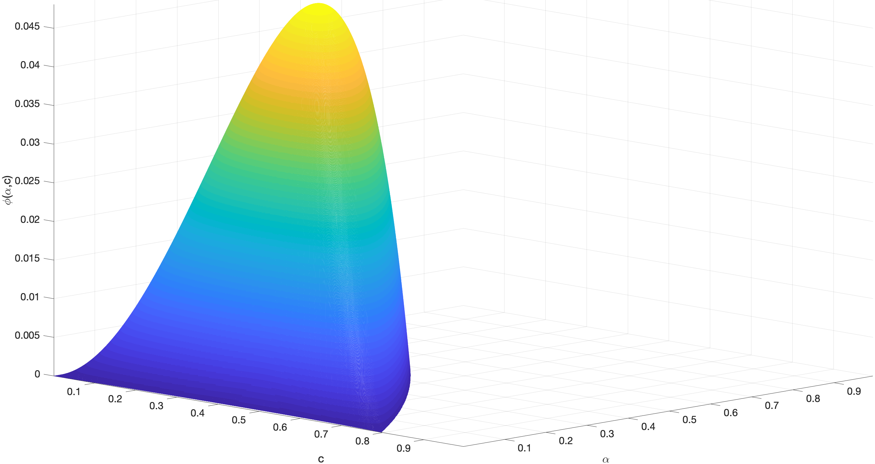
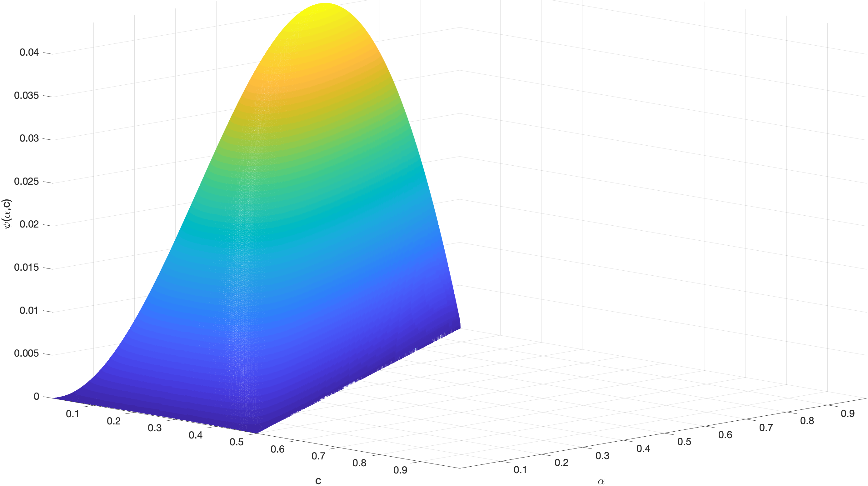
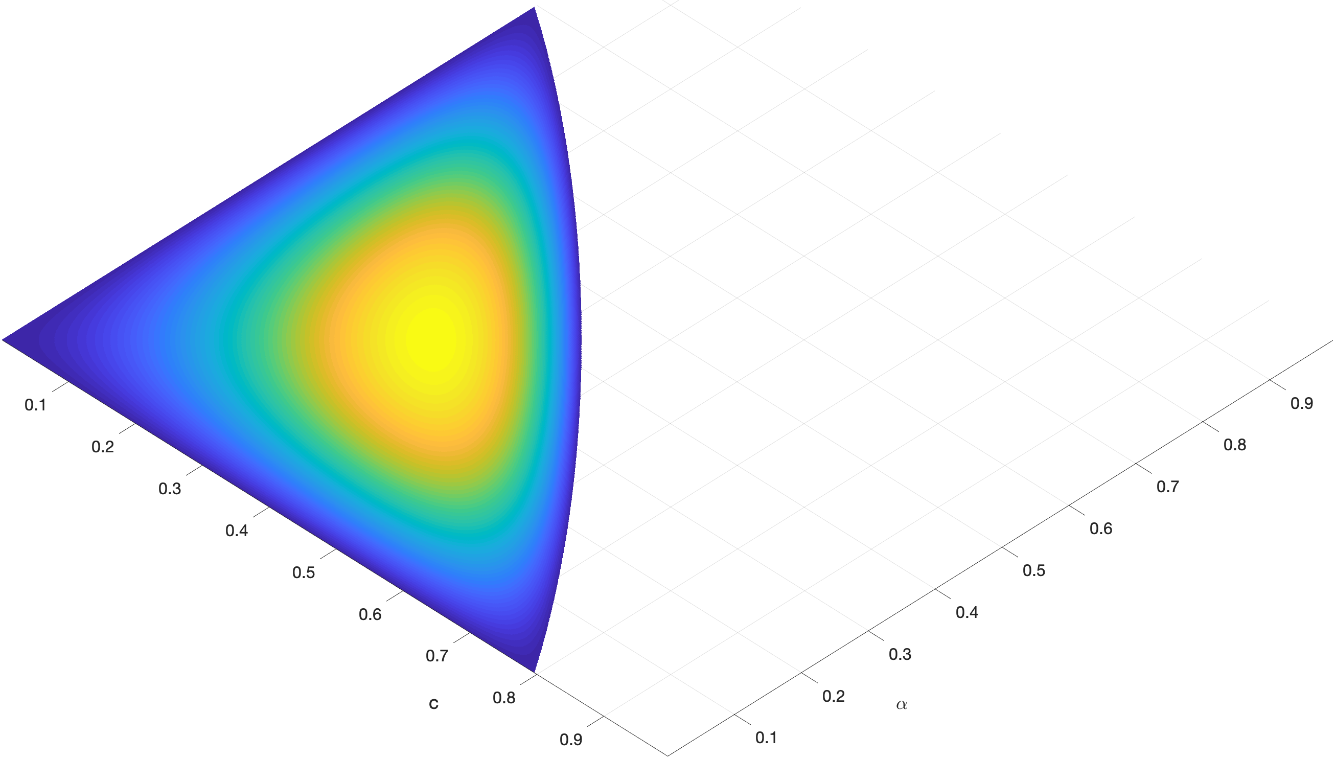
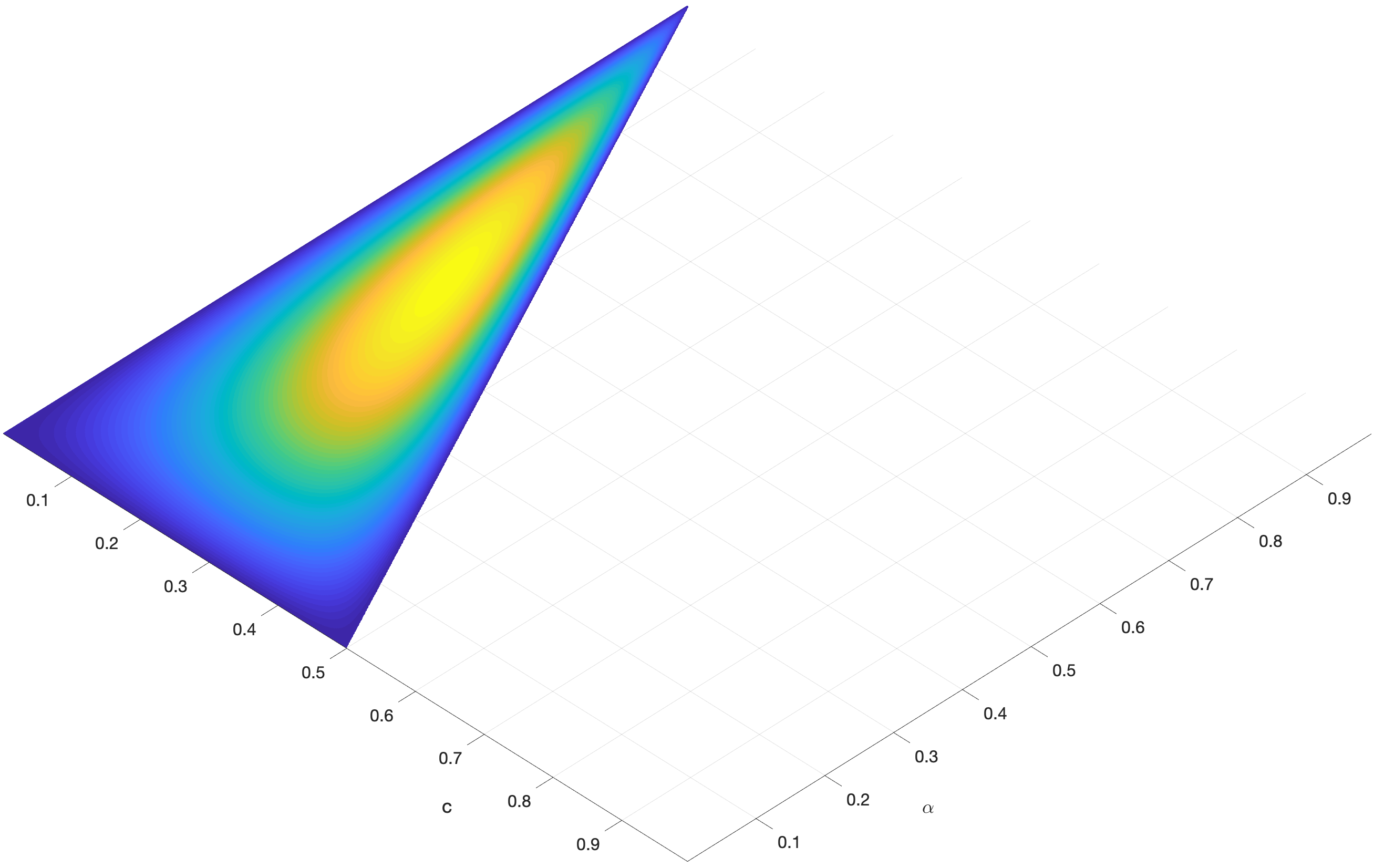
3D plots are presented in Figure 1 to illustrate the ranges of $\alpha$ and $c$ such that $\phi(\alpha,c)>0$ and $\psi(\alpha,c)>0$. This figure shows that large $\alpha$ and $c$ both result in overestimation of the true model. Moreover, Fujikoshi et al. (2014); Yanagihara et al. (2015) proved that for the fixed-$k$ case, the consistency ranges of $c$ for the AIC and $C_{p}$ are $[0,0.797)$ and $[0,1/2)$, respectively, which coincide with our results in Lemma 6.1 when $\alpha_{k}\to 0$.

Remark 3.5.

Combining Theorems 3.1 and 3.2, under an LLL asymptotic framework, if the BIC is strongly consistent, then the AIC is strongly consistent but not vice versa. This result contradicts the classical understanding that under a large-sample asymptotic framework, the AIC and $C_{p}$ are not consistent, but the BIC is strongly consistent.

Figure 1: 3D plots for $\phi(\alpha,c)>0$ and $\psi(\alpha,c)>0$. The left two figures are a wireframe mesh and a contour plot for $\phi(\alpha,c)>0$. The right two figures are a wireframe mesh and a contour plot for $\psi(\alpha,c)>0$.

3.2 KOO methods based on the AIC, BIC, and $C_{p}$

The AIC, BIC, and $C_{p}$ become computationally complex as $k$ becomes large because we must compute a minimum of $2^{k}-1$ statistics. An alternate procedure, which was introduced by Zhao et al. (1986) and Nishii et al. (1988) and implemented by Fujikoshi and Sakurai (2018), is available to avoid this problem. In the following, we examine the performance of this procedure under an LLL framework. Denote

$$\tilde{A}_{j} :=\frac{1}{n}(A_{{\bm{\omega}}\backslash j}-A_{{\bm{\omega}}})=\log(|\widehat{\mbox{\boldmath$\Sigma$}}_{{\bm{\omega}}\backslash j}|)-\log(|\widehat{\mbox{\boldmath$\Sigma$}}_{{\bm{\omega}}}|)-2c_{n},$$

$$\tilde{B}_{j} :=\frac{1}{n}(B_{{\bm{\omega}}\backslash j}-B_{{\bm{\omega}}})=\log(|\widehat{\mbox{\boldmath$\Sigma$}}_{{\bm{\omega}}\backslash j}|)-\log(|\widehat{\mbox{\boldmath$\Sigma$}}_{{\bm{\omega}}}|)-\log(n)c_{n},$$

$$\tilde{C}_{j} :=\frac{1}{n}(C_{{\bm{\omega}}\backslash j}-C_{{\bm{\omega}}})=(1-\alpha_{k}){\rm tr}(\widehat{\mbox{\boldmath$\Sigma$}}_{{\bm{\omega}}}^{-1}\widehat{\mbox{\boldmath$\Sigma$}}_{{\bm{\omega}}\backslash j})-(n-k+2)c_{n}.$$

Choose the model

$$\tilde{\bf j}_{A}=\{j\in{\bm{\omega}}|\tilde{A}_{j}>0\},~{}~{}~{}\tilde{\bf j}_{B}=\{j\in{\bm{\omega}}|\tilde{B}_{j}>0\}$$

$$\tilde{\bf j}_{C}=\{j\in{\bm{\omega}}|\tilde{C}_{j}>0\}.$$

These methods are based on the comparison of two models, models $M_{\bm{\omega}\backslash j}$ and $M_{\bm{\omega}}$; therefore, selection methods $\tilde{{\bf j}}_{A}$, $\tilde{{\bf j}}_{B}$ and $\tilde{{\bf j}}_{C}$ are referred to as kick-one-out (KOO) methods based on the AIC, BIC and $C_{p}$, respectively.

Note that the $-2\log$ likelihood ratio statistic for testing $\bm{\theta}_{j}=\bf 0$ under normality can be expressed as

$$n\left\{\log(|\hat{\Sigma}_{\bm{\omega}}|)-\log(|\hat{\Sigma}_{\bm{\omega}/j}|)\right\}.$$

Similarly, $(n-k){\rm{tr}}(\hat{\Sigma}_{\bm{\omega}}^{-1}\hat{\Sigma}_{\bm{\omega}\backslash j})$ is the Lawley-Hotelling trace statistic for testing $\bm{\theta}_{j}=\bf 0$. Here, $\tilde{A}_{j}$ $(\tilde{B}_{j},~{}\tilde{C}_{j})$ is regarded as a measure that expresses the degree of contribution of $\bf x_{j}$ based on $A_{j}$ $(B_{j},~{}C_{p})$. As such, the KOO methods may also be referred to as test-based methods, as in Fujikoshi and Sakurai (2018). Therefore, we have the following theorem for the KOO methods.

Theorem 3.6.

Suppose assumptions (A1) through (A5) hold.

• If for any $j\in{\bf j}_{*}$, $\log(\tau_{{\bm{\omega}}\backslash j})>\log(1-\alpha-c)+2c$, then

  • if $\log(\frac{1-\alpha}{1-\alpha-c})<2c$, the KOO method based on the AIC is strongly consistent;

  • if $\log(\frac{1-\alpha}{1-\alpha-c})>2c$, the KOO method based on the AIC is almost surely overspecified.

  If for some $j\in{\bf j}_{*}$, $\log(\tau_{{\bm{\omega}}\backslash j})<\log(1-\alpha-c)+2c$, then the KOO method based on the AIC is almost surely underspecified.

• The KOO method based on the BIC is almost surely underspecified.

• If for any $j\in{\bf j}_{*}$, $\kappa_{{\bm{\omega}}\backslash j}>\frac{c(1-\alpha-2c)}{1-\alpha}$, then

  • if $(1-\alpha)<2(1-\alpha-c)$, the KOO method based on the $C_{p}$ is strongly consistent.

  • if $(1-\alpha)>2(1-\alpha-c)$, the KOO method based on $C_{p}$ is almost surely overspecified.

  If for some $j\in{\bf j}_{*}$, $\kappa_{{\bm{\omega}}\backslash j}<\frac{c(1-\alpha-2c)}{1-\alpha}$, then the KOO method based on the $C_{p}$ is almost surely underspecified.

Suppose that assumptions (A1) through (A4) and (A5’) hold.

• If $\log(\frac{1-\alpha}{1-\alpha-c})<2c$, the KOO method based on the AIC is strongly consistent. Otherwise, if $\log(\frac{1-\alpha}{1-\alpha-c})>2c$, the KOO method based on the AIC is almost surely overspecified.

• If for any $j\in{\bf j}_{*}$, $\lim_{p,n}[\log(\tau_{n{\bm{\omega}}\backslash j})-\log(n)c]>\log(1-\alpha-c),$ then

  • if $\log(\frac{1-\alpha}{1-\alpha-c})<2c$, the KOO method based on the BIC is strongly consistent;

  • if $\log(\frac{1-\alpha}{1-\alpha-c})>2c$, the KOO method based on the BIC is almost surely overspecified.

  If for some $j\in{\bf j}_{*}$, $\lim_{p,n}[\log(\tau_{n{\bm{\omega}}\backslash j})-\log(n)c]<\log(1-\alpha-c),$ then the KOO method based on the BIC is almost surely underspecified.

• If $(1-\alpha)<2(1-\alpha-c)$, then the KOO method based on the $C_{p}$ is strongly consistent. Otherwise, if $(1-\alpha)>2(1-\alpha-c)$, the KOO method based on the AIC is almost surely overspecified.

The proof of this theorem is presented in Section 6.

Remark 3.7.

When the dimension $p$ and model size $k$ are fixed but the sample size $n\to\infty$, the asymptotic performance of the KOO methods and the classical AIC and BIC procedures are the same, as described by Nishii et al. (1988). However, according to Theorems 3.1 and 3.6, when $p$ and $k$ are large, the conditions for the KOO methods based on the AIC, BIC, and $C_{p}$ are stronger than those based on the classical AIC, BIC, and $C_{p}$. The reason is that the KOO methods are compared with the full model, whereas the classical AIC, BIC, and $C_{p}$ are compared with the true model. When the full model size is large and the true model size is small, the methods have different properties.

3.3 General KOO methods

In the classical AIC, BIC, and $C_{p}$, including the KOO methods based on the AIC, BIC, and $C_{p}$, the penalty terms are important and modified by many researchers. For the classical information criteria under a large-sample asymptotic framework, Nishii et al. (1988) proved that the strong consistency must be on the order of the penalty larger than $O(\log\log n)$ and smaller than $O(n)$, which coincides with the fact that the AIC is not consistent and the BIC is strongly consistent. However, on the basis of the above results, under an LLL framework, a large penalty may cause incorrect selection (actually, a constant penalty is sufficient for strong consistency), and the ranges of $\alpha$ and $c$ may be crucial for the consistency. Thus, we consider a new criterion that is independent of the penalty and reduces the conditions for $\alpha$ and $c$. Therefore, in this subsection, we propose two general KOO methods based on the likelihood ratio statistic and the Lawley-Hotelling trace statistic.

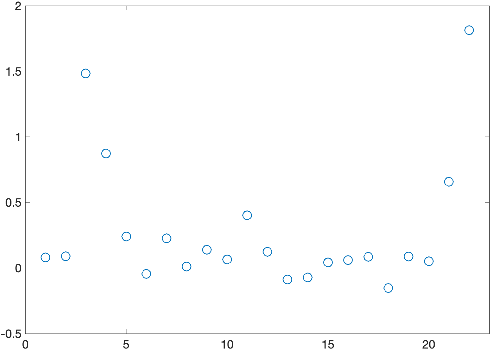
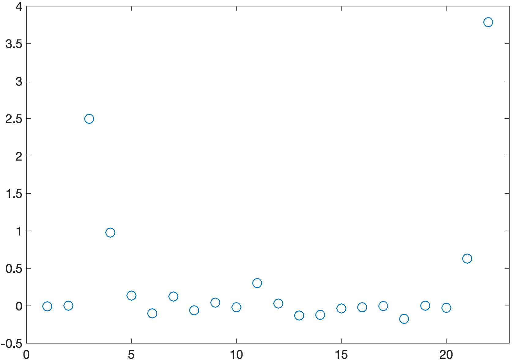
From the proof of Theorem 3.6, we find that the differences in the limits of $\tilde{A}_{j}$ for $j$ that exist and do not exist in the true model ${\bf j}_{*}$ are the two terms $\log(\tau_{{\bm{\omega}}\backslash j})$ and $\log(1-\alpha)$ (see (6.14) and (6.15)). That means if $\min_{j\in{\bf j}_{*}}\{\tau_{{\bm{\omega}}\backslash j}\}>1-\alpha$, for large enough $\{k,p,n\}$, the $k$ values of $\tilde{A}_{j}$ should be separated by a critical point and all the $\{\tilde{A}_{j}|j\in{\bf j}_{*}\}$ are the outliers because $k_{*}$ is fixed. The $k$ values of $\tilde{C}_{j}$ are analogous. We provide a numerical example in Figure 2 to illustrate the performances of $\{\tilde{A}_{j}\}$ and $\{\tilde{C}_{j}\}$ more clearly. In this case, the use of $Z_{1}$ and $Z_{2}$ as the critical points is not reasonable apparently.

(a) Histogram of $\breve{A}_{j}$

(b) Histogram of $\breve{C}_{j}$

Figure 2: We chose a Gaussian sample with $p=600$, $n=1500$, $k=450$ and $k_{*}=5$. Hence, $c=0.4$ and $\alpha=0.3$. The histograms represent the distributions of the $k$ values of $\breve{A}_{j}$ and $\breve{C}_{j}$ respectively. Here $Z_{1}=0$ and $Z_{2}=0$ represent the critical points of the KOO method based on AIC and $C_{p}$ respectively. $M_{1}=\log((1-\alpha)/(1-\alpha-c))$ and $M_{2}=p+c/(1-\alpha-c)$ are the limits of $\breve{A}_{j}$ and $\breve{C}_{j}$ respectively when $j$ does not lie in the true model.

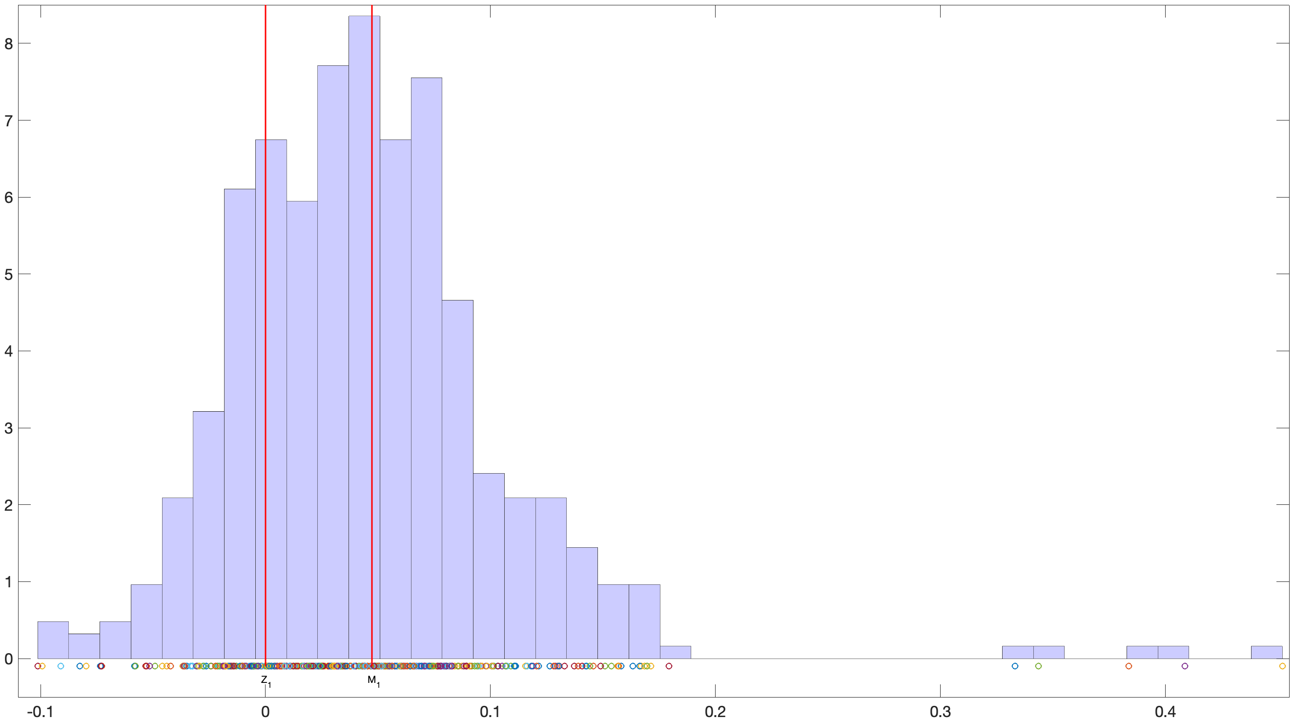
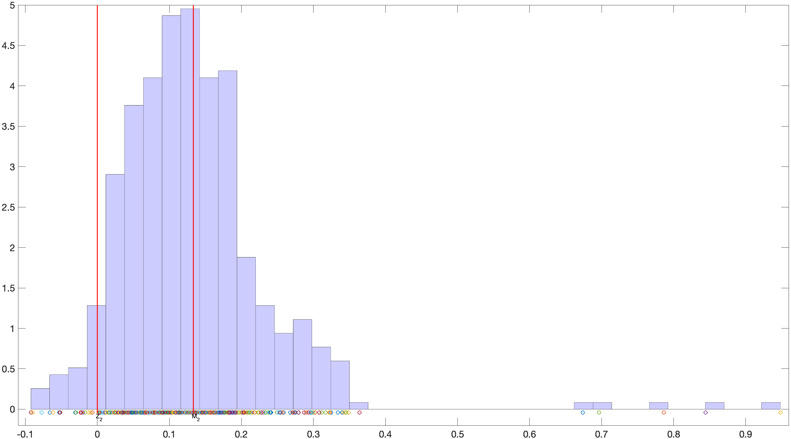
Thus, on the basis of these properties, we propose the following methods which are called the general KOO methods in the sequel. Denote

$$\breve{A}_{j}:=\log(|\widehat{\mbox{\boldmath$\Sigma$}}_{{\bm{\omega}}\backslash j}|)-\log(|\widehat{\mbox{\boldmath$\Sigma$}}_{{\bm{\omega}}}|)~{}~{}\mbox{and}~{}~{}\breve{C}_{j}:={\rm{tr}}(\widehat{\mbox{\boldmath$\Sigma$}}_{{\bm{\omega}}\backslash j}\widehat{\mbox{\boldmath$\Sigma$}}_{{\bm{\omega}}}^{-1}),$$

and a fixed value $\vartheta\in(0,\min_{j\in{\bf j}_{*}}\{\kappa_{{\bm{\omega}}\backslash j}\})$, choose the model

$$\breve{\bf j}_{A}=\{j\in{\bm{\omega}}|\breve{A}_{j}>\log(\frac{1-\alpha+\vartheta}{1-\alpha-c})\},~{}~{}~{}\breve{\bf j}_{C}=\{j\in{\bm{\omega}}|\breve{C}_{j}>\frac{\vartheta+c}{1-\alpha-c}+p\}.$$

Then, we have the following theorem.

Theorem 3.8.

Suppose assumptions (A1) through (A4) hold and that for any $j\in{\bf j}_{*}$, $\kappa_{{\bm{\omega}}\backslash j}>0$. Then, for any fixed value $\vartheta\in(0,\min_{j\in{\bf j}_{*}}\{\kappa_{{\bm{\omega}}\backslash j}\})$, the general KOO methods are strongly consistent, i.e.,

$$\lim_{n,p\to\infty}\breve{{\bf j}}_{A}\stackrel{{\scriptstyle a.s.}}{{\to}}{\bf j}_{*}~{}~{}~{}\mbox{and}~{}~{}~{}\lim_{n,p\to\infty}\breve{{\bf j}}_{C}\stackrel{{\scriptstyle a.s.}}{{\to}}{\bf j}_{*}.$$

The proof of this theorem is presented in Section 6.

Remark 3.9.

Note that the condition in this theorem is much weaker than that in the AIC, BIC, and $C_{p}$ and in the KOO methods based on the AIC, BIC, and $C_{p}$. In addition, although $\kappa_{{\bm{\omega}}\backslash j}$ is not estimable for $j\in{\bf j}_{*}$, as the general KOO methods are essentially to detect the univariate outliers, thus there are many well developed methods can be used to determine the value of $\vartheta$ for application, such as the Standard Deviation (SD) method, Z-Score method, Tukey’s method, Median Absolute Deviation method and so on. Here we refer to (Barnett and Lewis, 1994) for more details.

4 Simulation studies

In this section, we numerically examine the validity of our claims. More precisely, we attempt to examine the consistency properties of the KOO methods and the general KOO methods based on the AIC, BIC, and $C_{p}$ in an LLL framework with different settings. The classical AIC, BIC, and $C_{p}$ procedures are not considered herein because of their computational challenges. We conduct a number of simulation studies to examine the effects of assumptions (A2), (A3), (A5) and (A5’) on the consistency of estimators $\tilde{\bf j}_{A}$, $\tilde{\bf j}_{B}$, $\tilde{\bf j}_{C}$, $\breve{\bf j}_{A}$, and $\breve{\bf j}_{C}$. Moreover, we are interested in gaining insight into the rate of convergence.

We consider the following two settings:

• Setting I: Fix $k_{*}=5$, $p/n=\{0.2,0.4,0.6\}$ and $k/n=\{0.1,0.2\}$ with several different values of $n$. Set ${\bf X}=(x_{ij})_{n\times k}$, $\Theta_{{\bf j}_{*}}=\sqrt{n}{\bf 1}_{5}{\bm{\theta}}_{*}$ and $\Theta=(\Theta_{{\bf j}_{*}},\bf{0})$, where $\{x_{ij}\}$ are i.i.d. generated from the continuous uniform distributions $U(1,5)$, ${\bf 1}_{5}$ is a five-dimensional vector of ones and ${\bm{\theta}}_{*}=((-0.5)^{0},\dots,(-0.5)^{p-1})$.

• Setting II: This setting is the same as Setting I, except $\Theta_{{\bf j}_{*}}=n{\bf 1}_{5}{\bm{\theta}}_{*}.$

We consider three cases for the distribution of ${\bf E}$: (i) a standard normal distribution; (ii) a standardized $t$ distribution with three degrees of freedom, i.e., $e_{ij}\sim t_{3}/\sqrt{Var(t_{3})}$; and (iii) a standardized chi-square distribution with two degrees of freedom, i.e., $e_{ij}\sim\chi^{2}_{2}/\sqrt{Var(\chi^{2}_{2})}$. Here we use the 2 SD method to choose the critical points in the general KOO methods, that are

$$\breve{\bf j}_{A}=\{j\in{\bm{\omega}}|\breve{A}_{j}>\log(\frac{1-\alpha}{1-\alpha-c})+2sd_{A}\}$$

and

$$\breve{\bf j}_{C}=\{j\in{\bm{\omega}}|\breve{C}_{j}>\frac{c}{1-\alpha-c}+p+2sd_{C}\},$$

where $sd_{A}$ and $sd_{C}$ are the sample standard deviations of $\{\breve{A}_{j}\}$ and $\{\breve{C}_{j}\}$ respectively.

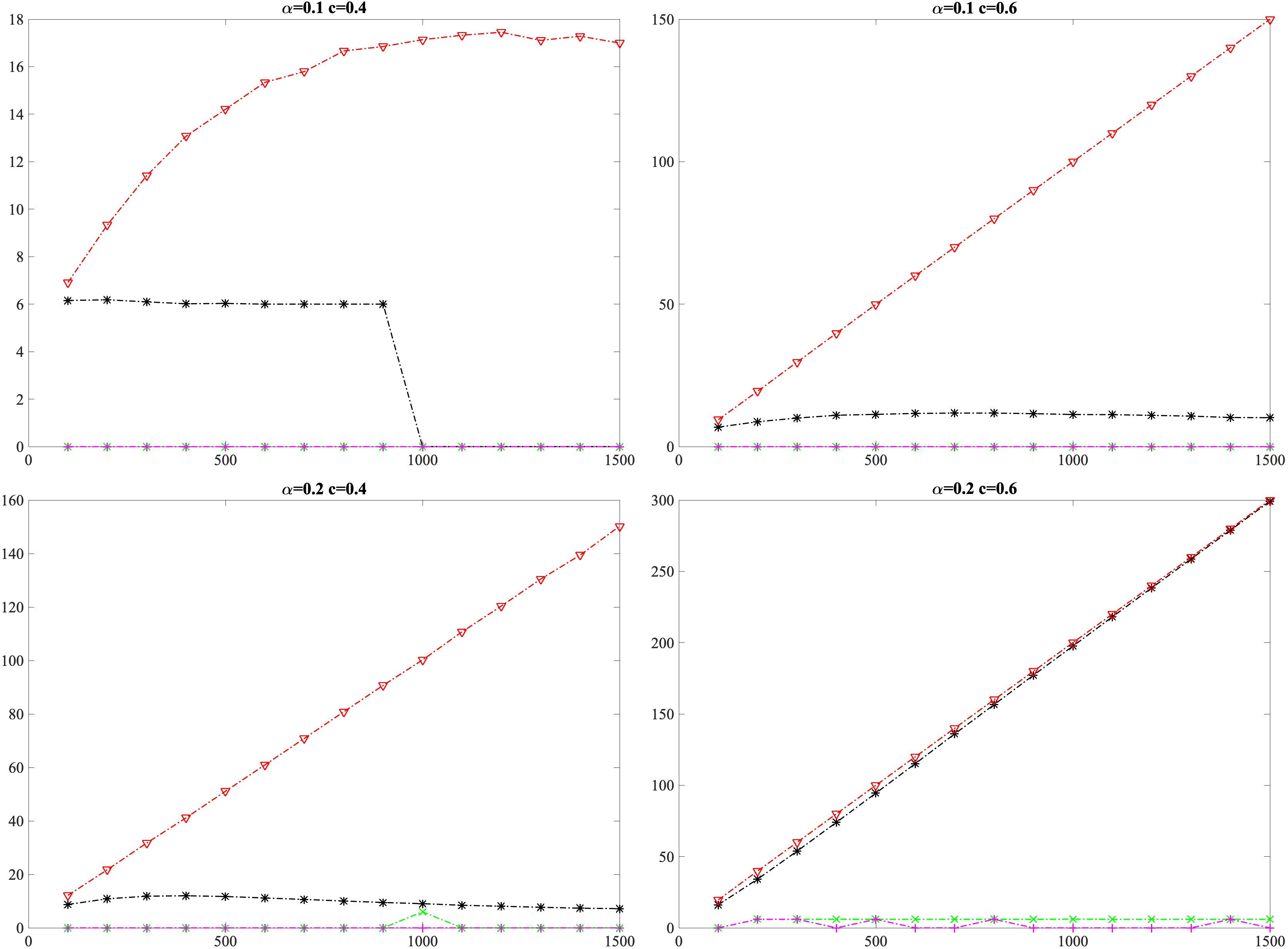
We highlight some salient features of our settings and the distributions. For Setting I, convergent values in the conditions for consistency are presented in Table 1 by simulation. From these values and Theorem 3.6, we know that $\tilde{\bf j}_{A}$ is strongly consistent in cases where $\{\alpha=0.1,c=0.2,0.4,0.6\}$ and $\{\alpha=0.2,c=0.2\}$. $\tilde{\bf j}_{C}$ is strongly consistent in cases where $\{\alpha=0.1,0.2,c=0.2\}$, and in other cases, $\tilde{\bf j}_{A}$, $\tilde{\bf j}_{B}$ and $\tilde{\bf j}_{C}$ are inconsistent. For Setting II, $\log(\tau_{{\bm{\omega}}\backslash\{1\}})=\log(n)+O(1)$ and $\kappa_{{\bm{\omega}}\backslash\{1\}}=O(n)$, which satisfy assumption (A5’). Under this setting, whether $\tilde{\bf j}_{B}$ is strongly consistent depends on the values of $c$ and $\alpha$.

	$c=.2$				$c=.4$				$c=.6$
	$V_{1}$	$V_{2}$	$V_{3}$	$V_{4}$	$V_{1}$	$V_{2}$	$V_{3}$	$V_{4}$	$V_{1}$	$V_{2}$	$V_{3}$	$V_{4}$
$\alpha=.1$	.15	.50	.87	1.49	.21	.10	.81	1.56	.10	-.30	.92	1.80
$\alpha=.2$	.11	.40	.91	1.32	.11	0	.92	1.43	-.19	-.40	1.21	1.72

Table 1: Values of $V_{1}:=2c-\log(\frac{1-\alpha}{1-\alpha-c})$, $V_{2}:=2(1-\alpha-c)-(1-\alpha)$, $V_{3}:=\log(\tau_{{\bm{\omega}}\backslash\{1\}})-\log(1-\alpha-c)-2c$, and $V_{4}:=\kappa_{{\bm{\omega}}\backslash\{1\}}-\frac{c(1-\alpha-2c)}{1-\alpha}$.

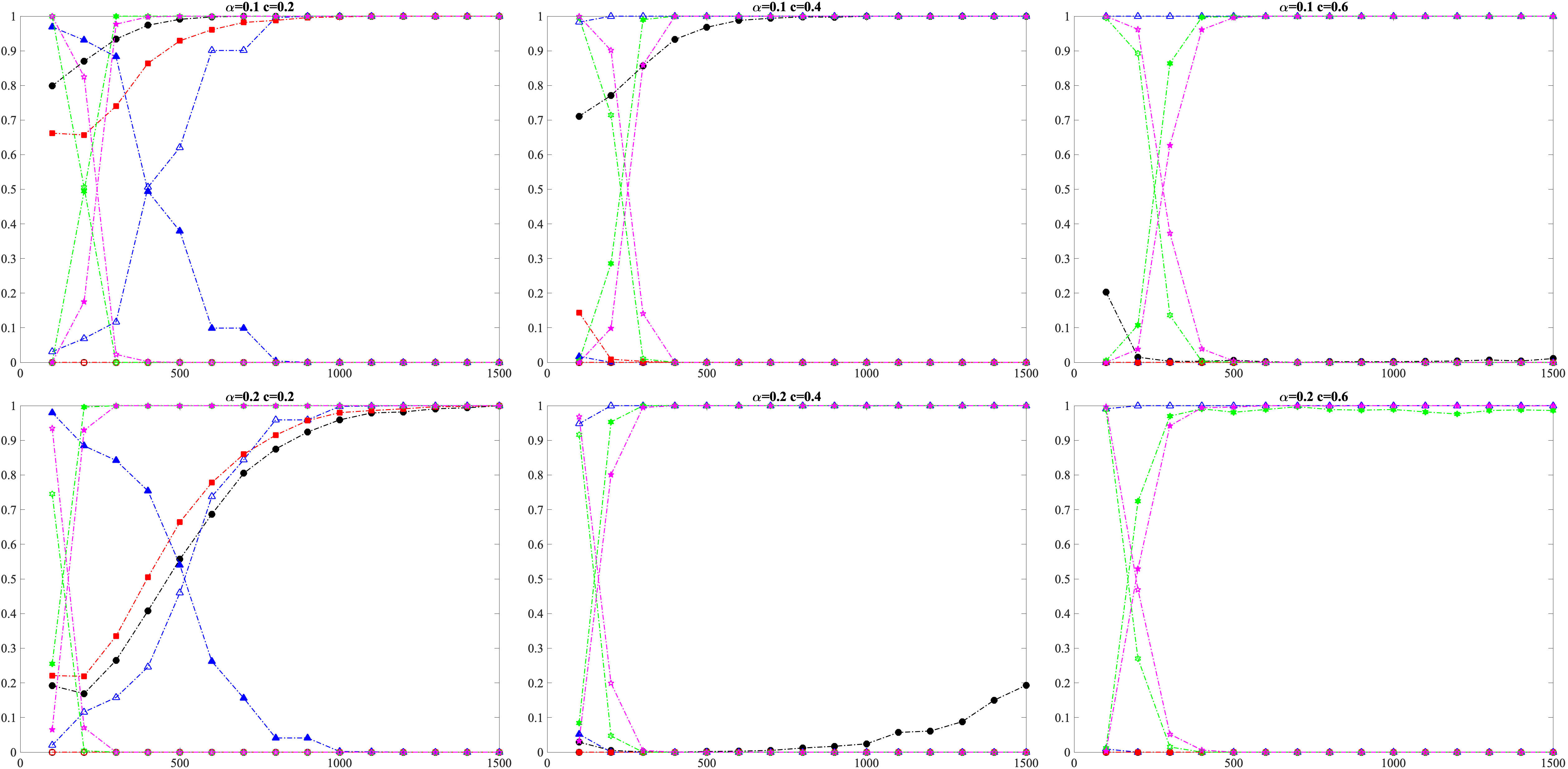
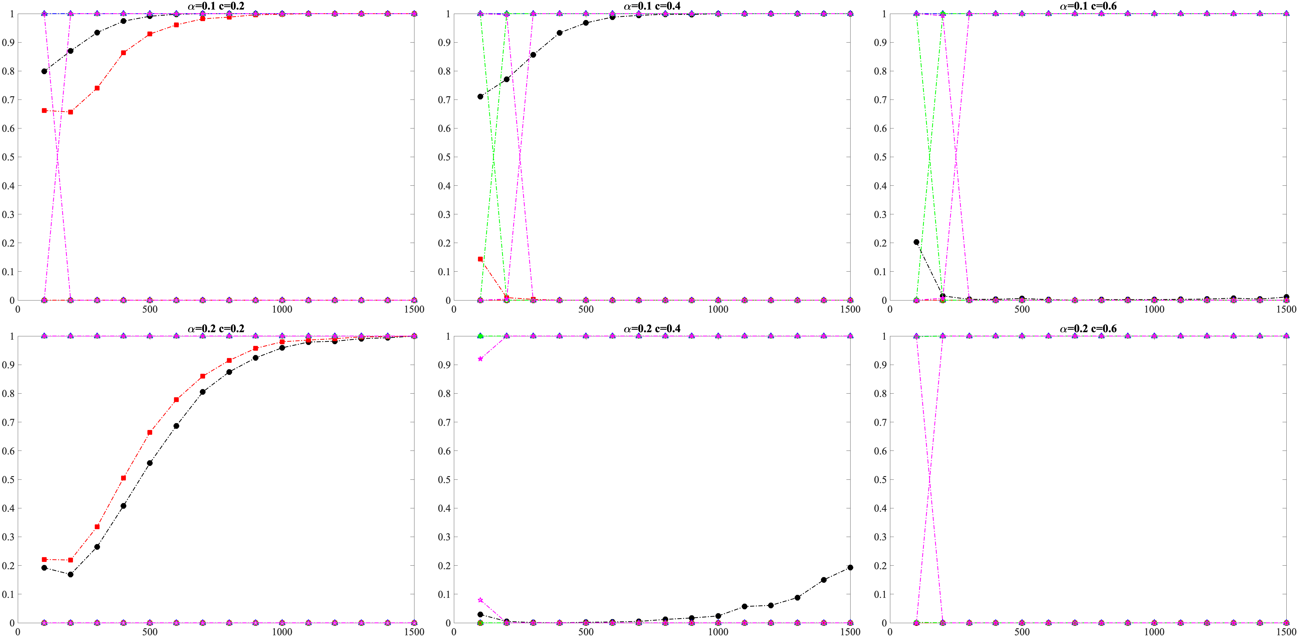
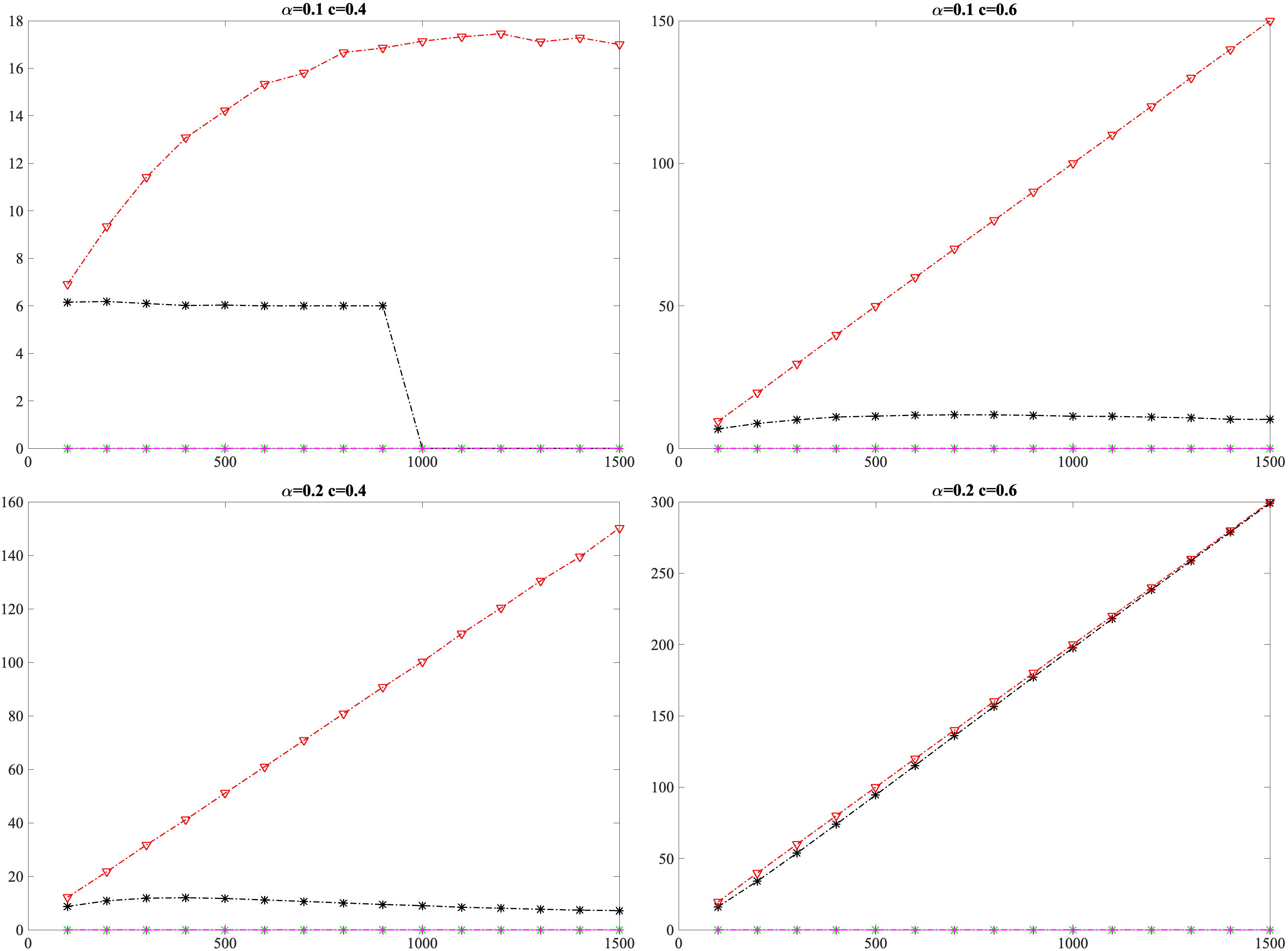
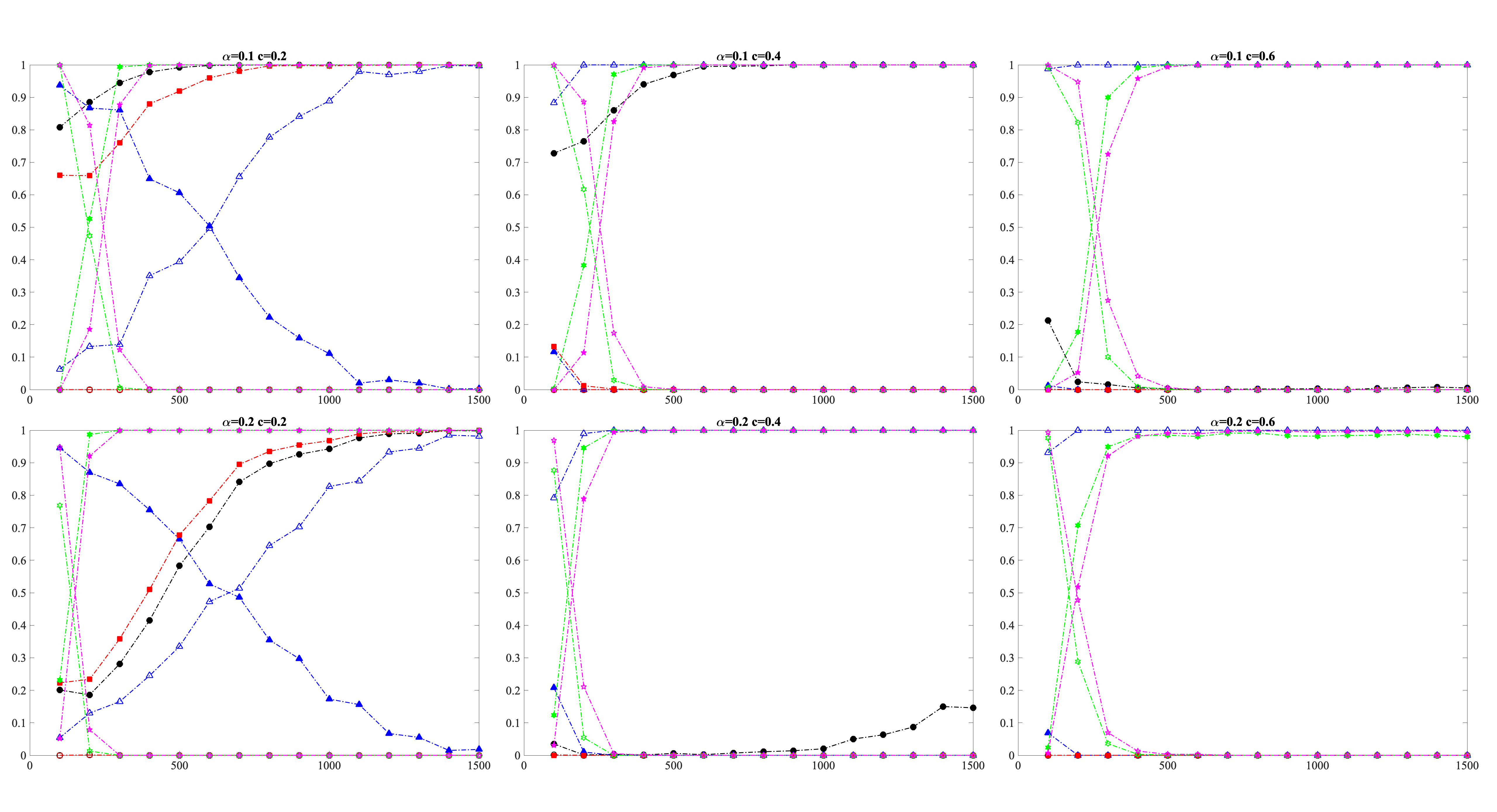
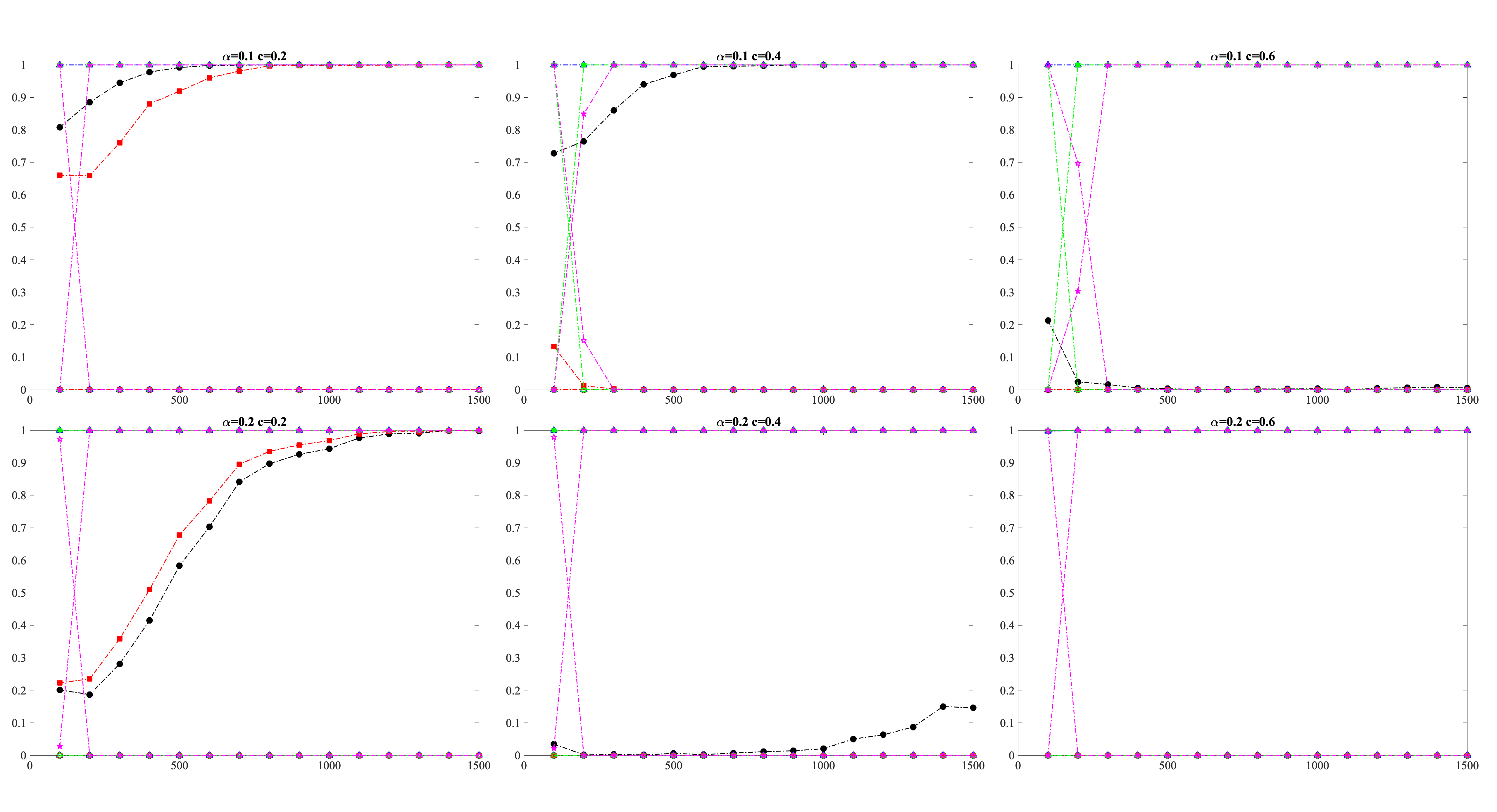
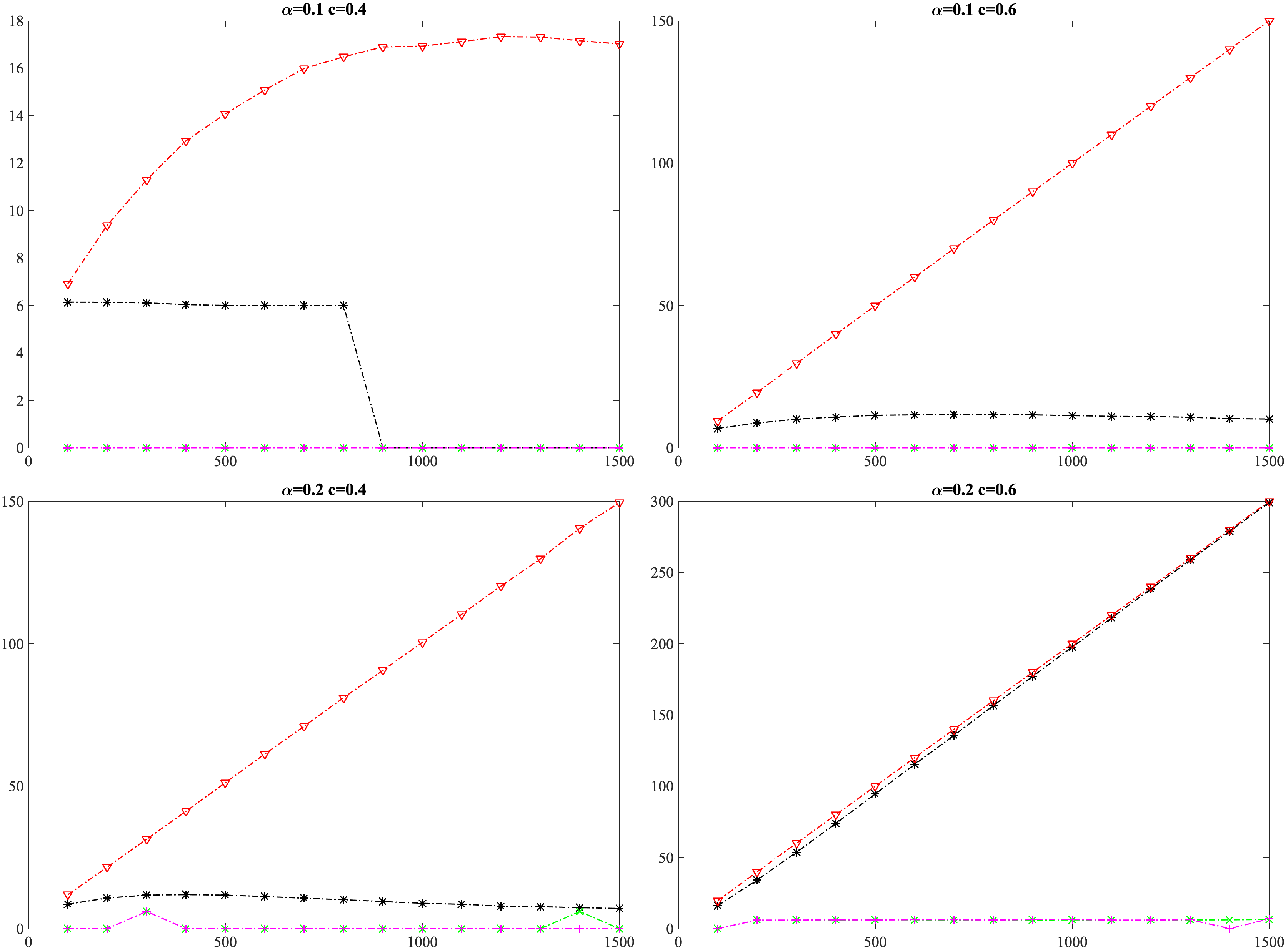
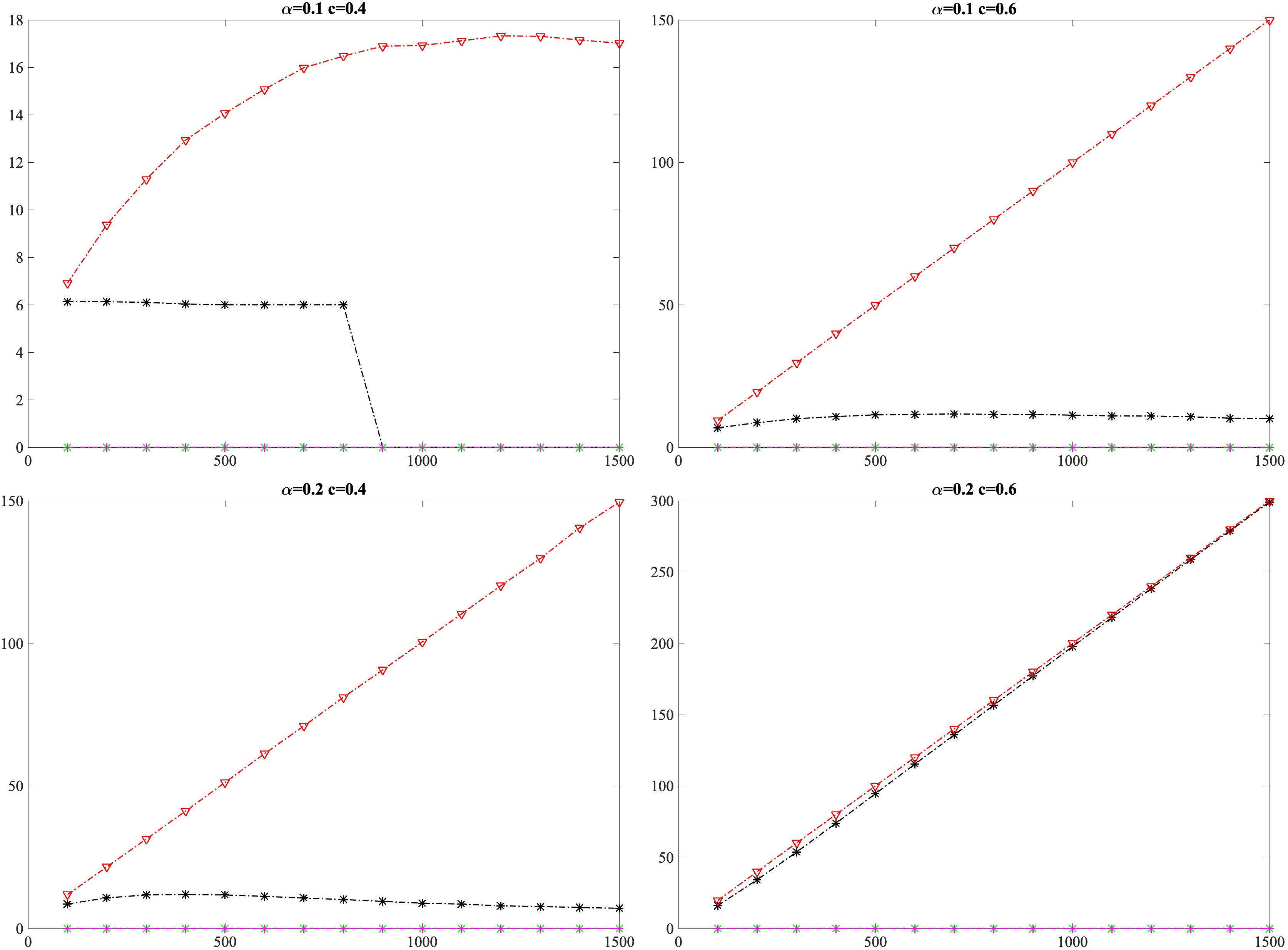
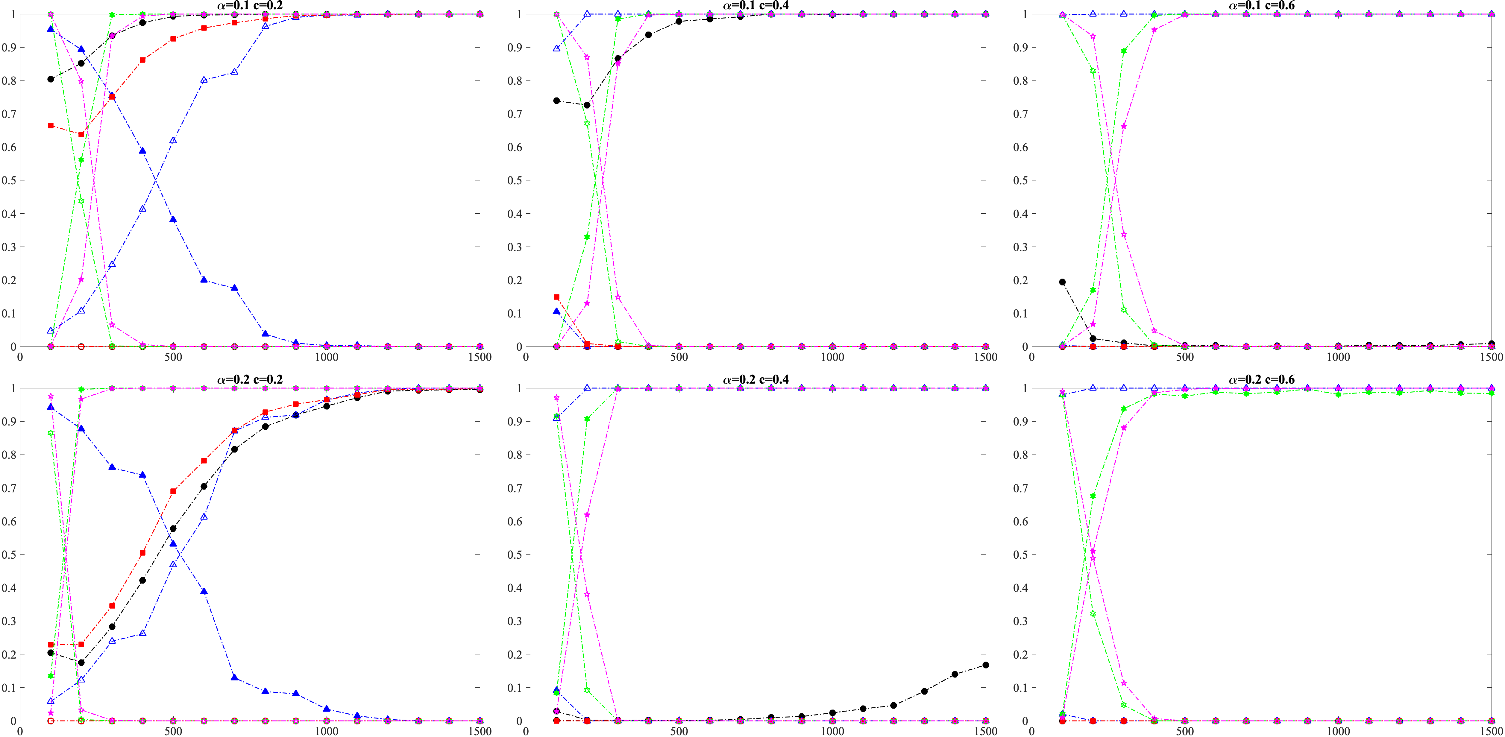
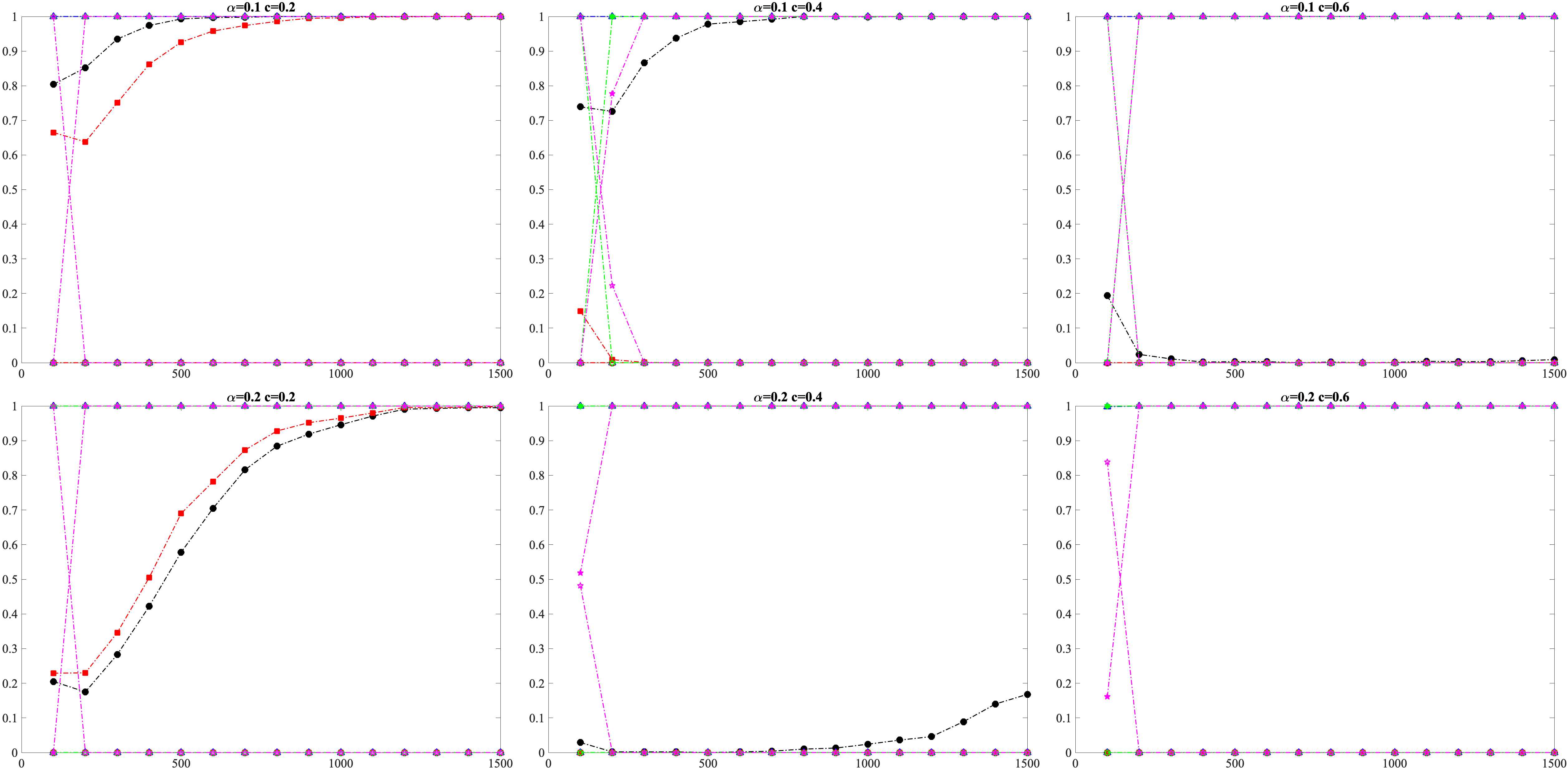
To illustrate the performance of these estimators, the selection percentages of belonging to ${\bf J}_{-}$, $\{{\bf j}_{*}\}$ and ${\bf J}_{+}$ were computed by Monte Carlo simulations with 1,000 repetitions. We first considered the standard normal distribution case. Since the sum of the three selection percentages is 1, for the sake of clarity of the plots, we display only the selection percentages of belonging to ${\bf J}_{-}$ and $\{{\bf j}_{*}\}$ (see Figure 3). Moreover, in some cases, when the selection percentages of belonging to ${\bf J}_{+}$ are close to 1, the selected model sizes are indicators of the consistency of the estimators, as presented in Figure 4. On the basis of these results, we have the following conclusions: (1) Under Setting I, the performances of the general KOO methods $\breve{\bf j}_{A}$ and $\breve{\bf j}_{C}$ are much better than those of the KOO methods $\tilde{\bf j}_{A}$, $\tilde{\bf j}_{B}$, and $\tilde{\bf j}_{C}$, and the sufficient conditions for the consistency of the KOO methods are satisfied. The convergence of $\tilde{\bf j}_{C}$ is the fastest among the five estimators. (2) If $c$ is large or close to the boundary of the sufficient conditions for consistency, i.e., $V_{1}$ and $V_{2}$ are small, then the convergence rate of the selection probabilities is slow, i.e., only sufficiently large samples can guarantee their selection accuracy. However, despite the low selection accuracy in this case, these methods usually overestimate the true model, and the selection sizes are also under control. An overspecified model is more acceptable than an underspecified model. (3) The KOO method based on the BIC performs the best among the three methods under Setting II, and when its sufficient conditions for consistency are satisfied. The reasons is that overestimating the true model by the BIC is difficult compared to overestimating the true model by the other criteria.

(a) Setting I

(b) Setting II

Figure 3: Selection percentages under AIC, BIC and $C_{p}$ for Settings I and II with a standard normal distribution. The horizontal axes represent the sample size $n$, and the vertical axes represent the selection percentages. Black solid circles, blue solid triangles, red solid squares, green solid hexagrams and magenta solid pentagrams denote the selection percentages of $\tilde{\bf j}_{A}={\bf j}_{*}$, $\tilde{\bf j}_{B}={\bf j}_{*}$, $\tilde{\bf j}_{C}={\bf j}_{*}$, $\breve{\bf j}_{A}={\bf j}_{*}$ and $\breve{\bf j}_{C}={\bf j}_{*}$, respectively. Correspondingly, black circles, blue triangles, red squares, green hexagrams, and magenta pentagrams denote the selection percentages of $\tilde{\bf j}_{A}\in{\bf J}_{-}$, $\tilde{\bf j}_{B}\in{\bf J}_{-}$, $\tilde{\bf j}_{C}\in{\bf J}_{-}$, $\breve{\bf j}_{A}\in{\bf J}_{-}$ and $\breve{\bf j}_{C}\in{\bf J}_{-}$, respectively.

(a) Setting I

(b) Setting II

Figure 4: Overspecified model sizes of AIC and $C_{p}$ for Settings I and II with a standard normal distribution. The horizontal axes represent the sample size $n$, and the vertical axes represent the model size. Black asterisks, red right-pointing triangles, green crosses and magenta plus signs denote the average sizes of $\tilde{\bf j}_{A}\in{\bf J}_{+}$, $\tilde{\bf j}_{C}\in{\bf J}_{+}$, $\breve{\bf j}_{A}\in{\bf J}_{+}$ and $\breve{\bf j}_{C}\in{\bf J}_{+}$, respectively. In this figure, we let $0/0=0$.

The results under non-normal distributions are similar to those under normal distributions. Please see Figures 7 through 10 in the Appendix, which verify our conclusion that the consistency of these estimators is independent of the distribution.

5 Real data analysis

For illustration, we apply the proposed methods to two real data examples. The first one is chemometrics data, which can be taken from Skagerberg et al. (1992) (we replaced the value 19203 with 1.9203 in the the 37th observation). This data set has been studied by Breiman and Friedman (1997); Similä and Tikka (2007). In this data set, There are $n=56$ observations with $k=22$ predictor variables and $p=6$ responses. The data are taken from a simulation of a low density tubular polyethylene reactor and to study the relationship between polymer properties and the process. The predictor variables consist of 20 temperatures measured at equal distances along the low density polyethylene reactor section together with the wall temperature of the reactor and the solvent feed rate. The responses are the output characteristics of the polymers including two molecular weights, two branching frequencies and the contents of two groups. Similar to Breiman and Friedman (1997), we log-transformed the responses values, because they are highly skewed to the right. By calculation, we get $\phi(\alpha_{n},c_{n})=0.0266$, $\psi(\alpha_{n},c_{n})=0.3444$, $2c-\log(\frac{1-\alpha_{n}}{1-\alpha_{n}-c_{n}})=0.0201$ and $2(1-\alpha_{n}-c_{n})-(1-\alpha_{n})=0.392$, which are all bigger than 0. Thus the AIC, BIC, $C_{p}$, KOO methods and general KOO methods are all applicable. We list the result in Table 2. For this dataset, we use the 1 SD method to choose the critical points in the general KOO methods, because there exist large extreme values in $\{\tilde{A}_{j}\}$ and $\{\tilde{C}_{j}\}$. We also present the scatterplots of $\{\tilde{A}_{j}\}$ and $\{\tilde{C}_{j}\}$ in Figure 5, and that seems the results obtained by the general KOO methods $\breve{\bf j}_{A}$ and $\breve{\bf j}_{C}$ are more reasonable than the KOO methods $\tilde{\bf j}_{A}$, $\tilde{\bf j}_{B}$ and $\tilde{\bf j}_{C}$.

Methods	Results
$\hat{\bf j}_{A}$	1, 2, 3, 4, 5, 7, 9, 10, 11, 12, 15, 16, 17, 19, 20, 21, 22
$\hat{\bf j}_{B}$	2, 3, 4, 5, 7, 11, 16, 17, 20, 21, 22
$\hat{\bf j}_{C}$	1, 3, 4, 5, 7, 9, 11, 12, 15, 16, 17, 19, 20, 21, 22
$\tilde{\bf j}_{A}$	1, 2, 3, 4, 5, 7, 8, 9, 10, 11, 12, 15, 16, 17, 19, 20, 21, 22
$\tilde{\bf j}_{B}$	3, 4, 5, 7, 11, 21, 22
$\tilde{\bf j}_{C}$	2, 3, 4, 5, 7, 9, 11 ,12, 21, 22
$\breve{\bf j}_{A}$	3, 4, 22
$\breve{\bf j}_{C}$	3, 4, 21, 22

Table 2: Selection results under the AIC, BIC, $C_{p}$, KOO methods and general KOO methods for the chemometrics dataset. Labels 1-20 are temperatures, 21 is the wall temperature and 22 is the solvent feed rate.

(a) Scatterplot of $\breve{A}_{j}$

(b) Scatterplotof $\breve{C}_{j}$

Figure 5: Scatterplots for the chemometrics dataset.

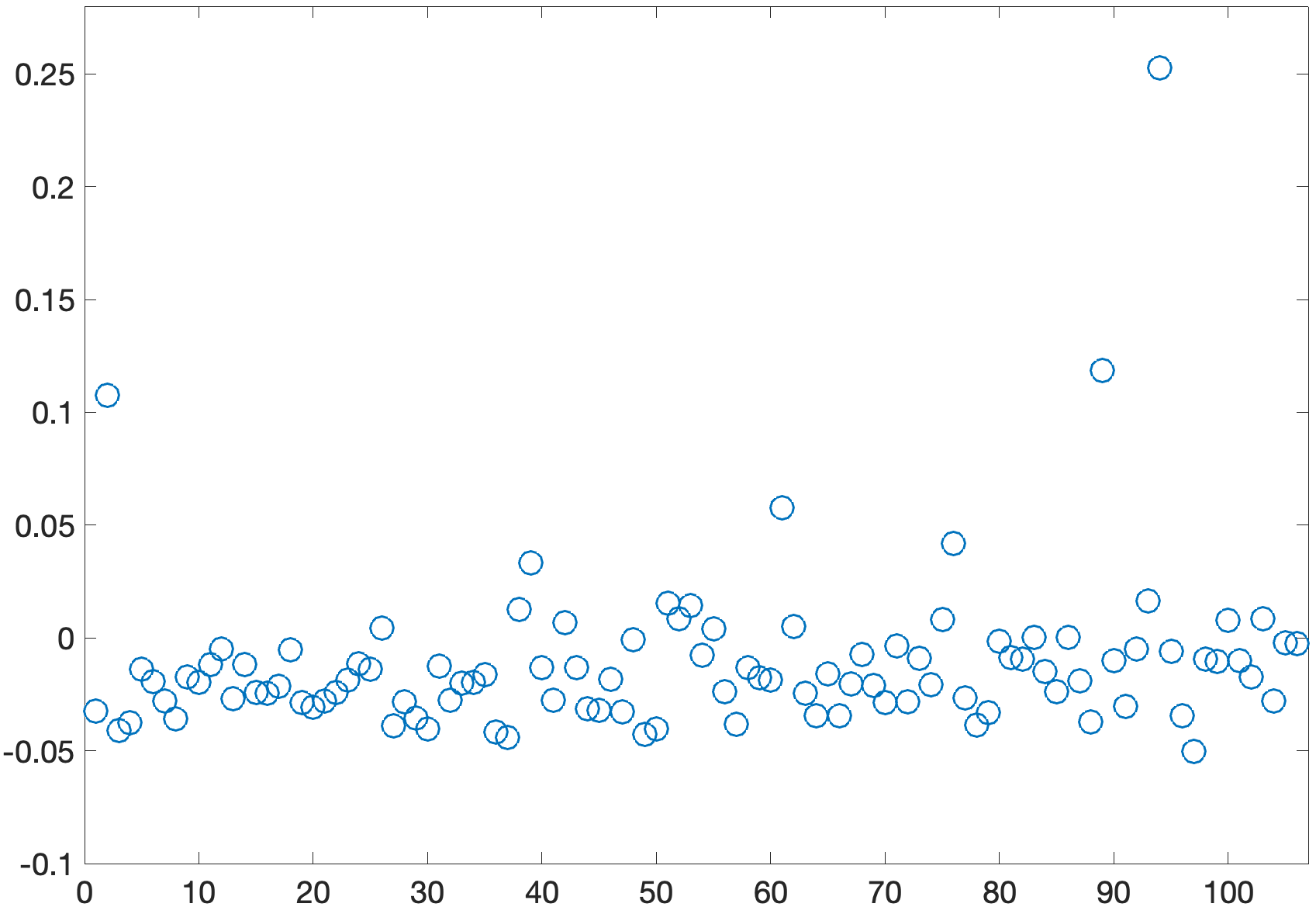
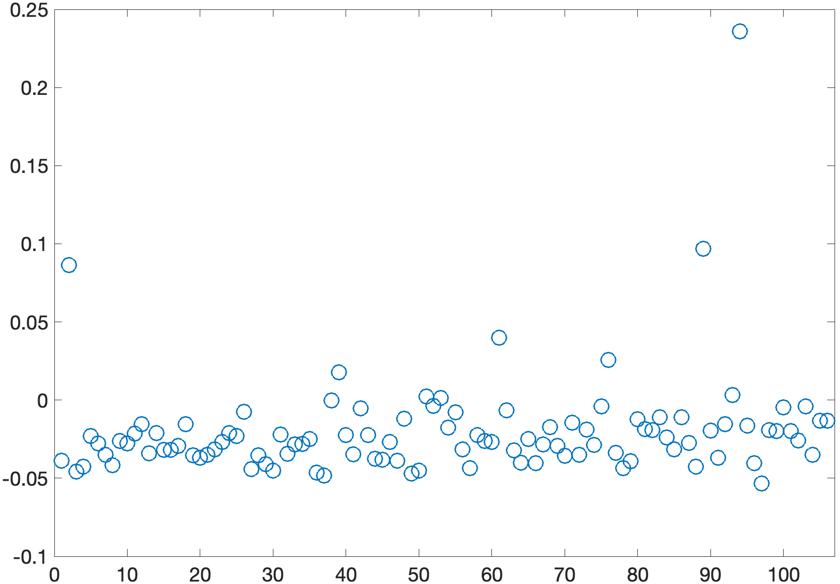
Analogously, we investigate a multivariate yeast cell-cycle dataset from Spellman et al. (1998), which can be obtained in the R package “spls”. This data set contains 542 cell-cycle-related genes (i.e., $n=542$). Each gene contains 106 binding levels of transcription factors (i.e., $k=106$) and 18 time points covering two cell cycles (i.e., $p=18$). The binding levels of the transcription factors play a role in determining which genes are expressed and help detail the process behind eukaryotic cellcycles. More explanations about the dataset can be found in (Wang et al., 2007; Chun and Keleş, 2010; Chen and Huang, 2012; Kong et al., 2017). As $2^{106}$ is too large to apply the classical methods based on the AIC, BIC and $C_{p}$, thus we only use KOO methods and general KOO methods for this dataset. The selection results are presented in Table 3, and the scatterplots of $\{\tilde{A}_{j}\}$ and $\{\tilde{C}_{j}\}$ can be found in Figure 6. The experimentally confirmed transcription factors that are related to the cell cycle regulation by Wang et al. (2007) are marked bold. These results also support our conclusion that the general KOO methods $\breve{\bf j}_{A}$ and $\breve{\bf j}_{C}$ are more reasonable than the KOO methods $\tilde{\bf j}_{A}$, $\tilde{\bf j}_{B}$ and $\tilde{\bf j}_{C}$.

Methods	Results
$\tilde{\bf j}_{A}$	SWI5, STE12, ACE2, NDD1, RME1, HIR2, SWI4, MBP1, MET31, HIR1,
	MCM1, YFL044C, RLM1, YAP5, IME4, NRG1, GAT3, MIG1, SIP4, SMP1
$\tilde{\bf j}_{B}$	SWI5
$\tilde{\bf j}_{C}$	SWI5, STE12, ACE2, NDD1, RME1, HIR2, SWI4, MBP1, MET31
$\breve{\bf j}_{A}$	SWI5, STE12, ACE2, NDD1, RME1, HIR2, SWI4, MBP1, MET31, HIR1
$\breve{\bf j}_{C}$	SWI5, STE12, ACE2, NDD1, RME1, HIR2, SWI4, MBP1

Table 3: Selection results under the KOO methods and general KOO methods for the yeast cell-cycle dataset. The experimentally confirmed transcription factors are marked bold.

(a) Scatterplot of $\breve{A}_{j}$

(b) Scatterplotof $\breve{C}_{j}$

Figure 6: Scatterplots for the yeast cell-cycle dataset.

6 Proofs of Theorems 3.1, 3.2, 3.6 and 3.8

In this section, we present the proofs of Theorems 3.1, 3.2, 3.6 and 3.8. We start with some preliminary results, which are not only the basis of the theorems but also have meaning themselves and have many potential applications in other multivariate analysis problems. In general, a $\{c_{n},\alpha_{k}\}$-dependent random variable $Z(c_{n},\alpha_{k})$ cannot serve as a limiting target of a random sequence $Z_{n}(c_{n},\alpha_{k}),n\geq 1$. Nevertheless, to ease the presentation, from time to time, without ambiguity we still write $Z_{n}(c_{n},\alpha_{k})\to Z(c_{n},\alpha_{k})$, if $Z_{n}(c_{n},\alpha_{k})-Z(c_{n},\alpha_{k})\to 0$.

6.1 Preliminaries

From the definition of the selection method based on the AIC, BIC, and $C_{p}$ in (1.3)-(1.7), the strong consistency of the selection method based on the AIC (resp. the BIC and $C_{p}$) is equivalent to that for all ${\bf j}\in{\bf J}\backslash{\bf j}_{*}$, $A_{{\bf j}}>A_{{\bf j}_{*}}$ (resp. $B_{{\bf j}}>B_{{\bf j}_{*}}$ and $C_{{\bf j}}>C_{{\bf j}_{*}}$) almost surely for sufficiently large $p$ and $n$. In addition, as ${\bf J}={\bf J}_{-}\cup{\bf j}_{*}\cup{\bf J}_{+}$, we need to consider only the following two cases, i.e., the overspecified case (${\bf j}\in{\bf J}_{+}$) and the underspecified case (${\bf j}\in{\bf J}_{-}$), and investigate for each case the conditions that guarantee that the inequality $A_{{\bf j}}>A_{{\bf j}_{*}}$ (resp. $B_{{\bf j}}>B_{{\bf j}_{*}}$ and $C_{{\bf j}}>C_{{\bf j}_{*}}$) holds. We first consider the overspecified case, i.e., ${\bf j}\in{\bf J}_{+}$, and assume that $k_{{\bf j}}-k_{{\bf j}_{*}}=m>0$; then, we have

$$\frac{1}{n}(A_{{\bf j}}-A_{{\bf j}_{*}})=\frac{1}{n}\sum_{t=0}^{m-1}(A_{{\bf j}_{-t}}-A_{{\bf j}_{-t-1}}).$$

Based on the definition of $A_{{\bf j}}$ in (1.3), it follows that

$$A_{{\bf j}_{-t}}-A_{{\bf j}_{-t-1}}=\log\left(\frac{|n\widehat{\mbox{\boldmath$\Sigma$}}_{{\bf j}_{-t}}|}{|n\widehat{\mbox{\boldmath$\Sigma$}}_{{\bf j}_{-t-1}}|}\right)+2c_{n},$$

which implies

$$\frac{1}{n}(A_{{\bf j}}-A_{{\bf j}_{*}})=\sum_{t=0}^{m-1}\left[\log\left(\frac{|n\widehat{\mbox{\boldmath$\Sigma$}}_{{\bf j}_{-t}}|}{|n\widehat{\mbox{\boldmath$\Sigma$}}_{{\bf j}_{-t-1}}|}\right)+2c_{n}\right].$$ (6.1)

Analogously, we also have

$$\frac{1}{n}(B_{{\bf j}}-B_{{\bf j}_{*}})=\sum_{t=0}^{m-1}\left[\log\left(\frac{|n\widehat{\mbox{\boldmath$\Sigma$}}_{{\bf j}_{-t}}|}{|n\widehat{\mbox{\boldmath$\Sigma$}}_{{\bf j}_{-t-1}}|}\right)+\log(n)c_{n}\right]$$ (6.2)

and

$$\frac{1}{n}(C_{{\bf j}}-C_{{\bf j}_{*}})= (1-\alpha_{k}){\rm tr}\widehat{[}{\mbox{\boldmath$\Sigma$}}_{{\bm{\omega}}}^{-1}(\widehat{\mbox{\boldmath$\Sigma$}}_{{\bf j}}-\widehat{\mbox{\boldmath$\Sigma$}}_{{\bf j}_{*}})]+2mc_{n}$$

$$= \sum_{t=0}^{m-1}\left((1-\alpha_{k}){\rm tr}[\widehat{\mbox{\boldmath$\Sigma$}}_{{\bm{\omega}}}^{-1}(\widehat{\mbox{\boldmath$\Sigma$}}_{{\bf j}_{-t}}-\widehat{\mbox{\boldmath$\Sigma$}}_{{\bf j}_{-t-1}})]+2c_{n}\right).$$ (6.3)

Then, we have the following lemma.

Lemma 6.1.

Suppose that assumptions (A1) through (A4) hold. For all overspecified models ${\bf j}$ with $k_{{\bf j}}-k_{{\bf j}_{*}}=m>0$, we have

$$\frac{1}{n}(A_{{\bf j}}-A_{{\bf j}_{*}})-\sum_{t=1}^{m}\log\left(\frac{1-\alpha_{m-t}-c_{n}}{1-\alpha_{m-t}}\right)-2mc_{n}=o_{a.s.}(m),$$ (6.4)

$$\frac{1}{n}(B_{{\bf j}}-B_{{\bf j}_{*}})-\sum_{t=1}^{m}\log\left(\frac{1-\alpha_{m-t}-c_{n}}{1-\alpha_{m-t}}\right)-mc_{n}\log(n)=o_{a.s.}(m)$$ (6.5)

and

$$\frac{1}{n}(C_{{\bf j}}-C_{{\bf j}_{*}})-\frac{mc_{n}(\alpha_{k}-1)}{1-\alpha_{k}-c_{n}}-2c_{n}m=o_{a.s.}(m).$$ (6.6)

Moreover, if $\lim_{n\to\infty}\alpha_{m}>0$, then we have

$$\frac{1}{n^{2}}(A_{{\bf j}}-A_{{\bf j}_{*}})=\phi(\alpha_{m},c_{n})+o_{a.s.}(1),$$ (6.7)

$$\frac{1}{n^{2}}(B_{{\bf j}}-B_{{\bf j}_{*}})-(\log(n)-2)c_{n}\alpha_{m}=\phi(\alpha_{m},c_{n})+o_{a.s.}(1),$$ (6.8)

and

$$\frac{1}{n^{2}}(C_{{\bf j}}-C_{{\bf j}_{*}})=\alpha_{m}\psi(\alpha_{k},c_{n})+o_{a.s.}(1).$$ (6.9)

The proof of this lemma needs RMT, thus we present it in Section 7 for understandability.

Remark 6.2.

Note that, taking the AIC for example, this lemma indicates that if $\lim\sum_{t=1}^{m}\log\left(\frac{1-\alpha_{m-t}-c_{n}}{1-\alpha_{m-t}}\right)+2mc_{n}>0$, for all ${\bf j}\in{\bf J}_{+}$ satisfying $k_{{\bf j}}-k_{{\bf j}_{*}}=m$ and sufficiently large $p$ and $n$, then ${\bf j}$ almost surely cannot be selected by the AIC. On the other hand, if $\lim\sum_{t=1}^{m}\log\left(\frac{1-\alpha_{m-t}-c_{n}}{1-\alpha_{m-t}}\right)+2mc_{n}<0$, then for sufficiently large $p$ and $n$, ${\bf j}_{*}$ almost surely cannot be selected by the AIC, which means that, in this case, the AIC is almost surely inconsistent. The BIC and $C_{p}$ are analogous.

Next, we consider the underspecified case, i.e., ${\bf j}\in{\bf J}_{-}$. Analogously, we have

$$\frac{1}{n}(A_{{\bf j}}-A_{{\bf j}_{*}})=\sum_{t=-s}^{m-1}{\mathcal{A}}_{-t},$$

$$\frac{1}{n}(B_{{\bf j}}-B_{{\bf j}_{*}})=\sum_{t=-s}^{m-1}{\mathcal{B}}_{-t}~{}~{}\mbox{and}~{}~{}\frac{1}{n}(C_{{\bf j}}-C_{{\bf j}_{*}})=\sum_{t=-s}^{m-1}{\mathcal{C}}_{-t},$$

where

$${\mathcal{A}}_{-t}=\begin{cases}\log({|\widehat{\mbox{\boldmath$\Sigma$}}_{{\bf j}_{-t}}|})-\log({|\widehat{\mbox{\boldmath$\Sigma$}}_{{\bf j}_{-t-1}}|})+2c_{n}&\mbox{if }t\geq 0,\\ \log({|\widehat{\mbox{\boldmath$\Sigma$}}_{{\bf j}_{-t}}|})-\log({|\widehat{\mbox{\boldmath$\Sigma$}}_{{\bf j}_{-t-1}}|})-2c_{n}&\mbox{if }t<0,\end{cases}$$

$${\mathcal{B}}_{-t}=\begin{cases}\log({|\widehat{\mbox{\boldmath$\Sigma$}}_{{\bf j}_{-t}}|})-\log({|\widehat{\mbox{\boldmath$\Sigma$}}_{{\bf j}_{-t-1}}|})+\log(n)c_{n}&\mbox{if }t\geq 0,\\ \log({|\widehat{\mbox{\boldmath$\Sigma$}}_{{\bf j}_{-t}}|})-\log({|\widehat{\mbox{\boldmath$\Sigma$}}_{{\bf j}_{-t-1}}|})-\log(n)c_{n}&\mbox{if }t<0,\end{cases}$$

and

$${\mathcal{C}}_{-t}=\begin{cases}(1-\alpha_{k}){\rm tr}[\widehat{\mbox{\boldmath$\Sigma$}}_{{\bm{\omega}}}^{-1}(\widehat{\mbox{\boldmath$\Sigma$}}_{{\bf j}_{-t}}-\widehat{\mbox{\boldmath$\Sigma$}}_{{\bf j}_{-t-1}})]+2c_{n}&\mbox{if }t\geq 0,\\ (1-\alpha_{k}){\rm tr}[\widehat{\mbox{\boldmath$\Sigma$}}_{{\bm{\omega}}}^{-1}(\widehat{\mbox{\boldmath$\Sigma$}}_{{\bf j}_{-t}}-\widehat{\mbox{\boldmath$\Sigma$}}_{{\bf j}_{-t-1}})]-2c_{n},&\mbox{if }t<0.\end{cases}$$

Since ${\bf j}_{0}\supset{\bf j}_{*}$, it from Lemma 6.1 that,

$$\sum_{t=0}^{m-1}{\mathcal{A}}_{-t}-\sum_{t=1}^{m}\log\left(\frac{1-\alpha_{m+s-t}-c_{n}}{1-\alpha_{m+s-t}}\right)-2mc_{n}=o_{a.s.}(m),$$

$$\sum_{t=0}^{m-1}{\mathcal{B}}_{-t}-\sum_{t=1}^{m}\log\left(\frac{1-\alpha_{m+s-t}-c_{n}}{1-\alpha_{m+s-t}}\right)-mc_{n}\log(n)=o_{a.s.}(m)$$

and

$$\sum_{t=0}^{m-1}{\mathcal{C}}_{-t}-m\psi(\alpha,c)=o_{a.s.}(m).$$

Therefore, we need to consider only the case in which $t<0$ and some additional notation. Let ${\mbox{\boldmath$\ell$}}_{t}=\{i_{1},\cdots,i_{-t}\}$, we denote

$$\Delta_{t}:= ({\bf X}^{\prime}_{{\mbox{\boldmath$\ell$}}_{t}}{\bf Q}_{{\bf j}_{t}}{\bf X}_{{\mbox{\boldmath$\ell$}}_{t}})^{1/2}\Theta_{{\mbox{\boldmath$\ell$}}_{t}}\Theta^{\prime}_{{\mbox{\boldmath$\ell$}}_{t}}({\bf X}^{\prime}_{{\mbox{\boldmath$\ell$}}_{t}}{\bf Q}_{{\bf j}_{t}}{\bf X}_{{\mbox{\boldmath$\ell$}}_{t}})^{1/2};$$

$$\tilde{\bf a}_{t}^{\prime}:= {\bf a}_{t}^{\prime}{\bf Q}_{{\bf j}_{t}}{\bf X}_{{\mbox{\boldmath$\ell$}}_{t}}({\bf X}_{{\mbox{\boldmath$\ell$}}_{t}}^{\prime}{\bf Q}_{{\bf j}_{t}}{\bf X}_{{\mbox{\boldmath$\ell$}}_{t}})^{-1/2};$$

$$\delta_{t}:= \tilde{\bf a}_{t}^{\prime}\left(({1-\alpha_{m}}){\bf I}+{n^{-1}\Delta_{t}}\right)^{-1}\tilde{\bf a}_{t};$$

$$\eta_{t}:= \frac{1}{n}\tilde{\bf a}_{t}^{\prime}\Delta_{t}\tilde{\bf a}_{t}=\frac{1}{n}{\bf a}_{t}^{\prime}{\bf Q}_{{\bf j}_{t}}{\bf X}_{{\mbox{\boldmath$\ell$}}_{t}}\Theta_{{\mbox{\boldmath$\ell$}}_{t}}\Theta^{\prime}_{{\mbox{\boldmath$\ell$}}_{t}}{\bf X}_{{\mbox{\boldmath$\ell$}}_{t}}^{\prime}{\bf Q}_{{\bf j}_{t}}{\bf a}_{t}.$$

By basic calculation, we obtain that $\delta_{t}$ and $\eta_{t}$ can both be expressed as functions of the noncentrality matrix $\Phi_{{\bf j}}$, as follows:

$$\prod_{l=1}^{-t}\tilde{\bf a}_{l}^{\prime}((1-\alpha_{m}){\bf I}+\frac{1}{n}\Delta_{l})^{-1}\tilde{\bf a}_{l}=(1-\alpha_{m})^{p+t}|(1-\alpha_{m}){\bf I}+\Phi_{{\bf j}}|^{-1}$$

and

$$\sum_{l=1}^{-t}\eta_{l}=\frac{1}{n}{\rm{tr}}[\Theta^{\prime}_{{\bf j}_{*}}{\bf X}_{{\bf j}_{*}}^{\prime}(\sum_{l=1}^{-t}{\bf a}_{l}{\bf a}_{l}^{\prime}){\bf X}_{{\bf j}_{*}}\Theta_{{\bf j}_{*}}]={\rm{tr}}(\Phi_{{\bf j}}).$$

Then, we have the following lemma.

Lemma 6.3.

Suppose assumptions (A1) through (A5) hold. If ${\bf j}\in{\bf J}_{-}$ and $t<0$, then we have

$${\mathcal{A}}_{-t}+\log({\delta_{t}})+\log({1-\alpha_{m}-c_{n}})+2c_{n}=o_{a.s.}(1),$$ (6.10)

$${\mathcal{B}}_{-t}+\log({\delta_{t}})+\log({1-\alpha_{m}-c_{n}})+c_{n}\log(n)=o_{a.s.}(1),$$ (6.11)

and

$${\mathcal{C}}_{-t}-\frac{(1-\alpha_{k})(\eta_{t}+c_{n})}{1-c_{n}-\alpha_{k}}+2c_{n}=o_{a.s.}(1).$$ (6.12)

The proof of this lemma is presented in Section 7. By combining Lemmas 6.1 and 6.3, the following lemma is straightforward.

Lemma 6.4.

Suppose that assumptions (A1) through (A5) hold. For all underspecified models ${\bf j}$ with $k_{{\bf j}_{-}}=s>0$ and $k_{{\bf j}_{+}}=m\geq 0$, we have

$$\frac{1}{n}(A_{{\bf j}}-A_{{\bf j}_{*}})= \sum_{t=1}^{m}\log\left(\frac{1-\alpha_{m+s-t}-c}{1-\alpha_{m+s-t}}\right)$$

$$+\log(\tau_{{\bf j}})-s\log({1-\alpha_{m}-c})+2(m-s)c+o_{a.s.}(m),$$

$$\frac{1}{n}(B_{{\bf j}}-B_{{\bf j}_{*}})= \sum_{t=1}^{m}\log\left(\frac{1-\alpha_{m+s-t}-c}{1-\alpha_{m+s-t}}\right)$$

$$+\log(\tau_{{\bf j}})-s\log({1-\alpha_{m}-c})+(m-s)c\log(n)+o_{a.s.}(m)$$

and

$$\frac{1}{n}(C_{{\bf j}}-C_{{\bf j}_{*}})=m\psi(\alpha,c)+\frac{(1-\alpha)(\kappa_{{\bf j}}+sc)}{1-c-\alpha}-2sc+o_{a.s.}(m).$$

Remark 6.5.

Lemmas 6.1 through 6.4 are the fundamental results for the model selection criteria discussed herein. These lemmas have numerous potential applications in multivariate analysis problems, such as the growth curve model (Enomoto et al., 2015; Fujikoshi et al., 2013), multiple discriminant analysis (Fujikoshi, 1983; Fujikoshi and Sakurai, 2016a), principal component analysis (Fujikoshi and Sakurai, 2016b; Bai et al., 2018), and canonical correlation analysis (Nishii et al., 1988; Bao et al., 2018).

Now, with the aid of Lemma 6.1 and Lemma 6.4, we prove Theorems 3.1, 3.2, 3.6 and 3.8.

6.2 Proof of Theorem 3.1

We first prove (1). For the strong consistency of AIC method, it is sufficient to prove for all ${\bf j}\neq{\bf j}_{*}$, $A_{{\bf j}}>A_{{\bf j}_{*}}$ almost surely for large enough $p$ and $n$. When ${\bf j}\in{\bf J}_{+}$ with $k_{{\bf j}}-k_{{\bf j}_{*}}=m$, from the definition of $\phi(\alpha,c)$, we know that if $\phi(\alpha,c)>0$, then we have $\log(1-c)+2c>0$, and for any $\alpha_{m}$ satisfying $0<\alpha_{m}\leq\alpha$, we have $\phi(\alpha_{m},c)>0$. In addition, if $\alpha_{m}\to 0$, by (6.7), we have

$$\frac{1}{nm}(A_{{\bf j}}-A_{{\bf j}_{*}})\stackrel{{\scriptstyle a.s.}}{{\to}}\log(1-c)+2c>0.$$

Thus, according to Lemma 6.1, if $\phi(\alpha,c)>0$, AIC method cannot be asymptoticly over-specified, i.e., for any ${\bf j}\in{\bf J}_{+}$ and for sufficiently large $p$ and $n$,

$$A_{{\bf j}}>A_{{\bf j}_{*}}~{}~{}~{}a.s..$$

For the case of ${\bf j}\in{\bf J}_{-}$ with $k_{{\bf j}_{+}}=m\geq 0$ and $k_{{\bf j}_{*}\cap{\bf j}_{-}^{c}}=s>0$, note that $s<k_{*}$, $\Phi_{{\bf j}}>0$ and $\log(\tau_{n{\bf j}})>s\log(1-\alpha_{m})$ uniformly. If $m\geq s$, by Lemma 6.4 and when $\phi(\alpha,c)>0$,

$$\frac{1}{n}(A_{{\bf j}}-A_{{\bf j}_{*}})$$

$$= \sum_{t=1}^{m}\log\left(\frac{1-\alpha_{m-t}-c}{1-\alpha_{m-t}}\right)$$

$$+\log(\tau_{{\bf j}})-s\log({1-\alpha_{m}-c})+2(m-s)c+o_{a.s.}(m)$$

$$= \sum_{t=s+1}^{m}\log\left(\frac{1-\alpha_{m-t}-c}{1-\alpha_{m-t}}\right)+\log(\tau_{{\bf j}}/(1-\alpha_{m}))+2(m-s)c+o_{a.s.}(m),$$

which is almost surely positive for sufficiently large $p$ and $n$. Thus, we only need to consider the case in which $m<s$. In this case, since $k_{*}$ is fixed, $\alpha_{m}=m/n\to 0$ and $\tau_{{\bf j}}>1$. Then, under the condition $\log(\tau_{{\bf j}})>(s-m)(\log(1-c)+2c)$, we have that

$$\frac{1}{n}(A_{{\bf j}}-A_{{\bf j}_{*}})\stackrel{{\scriptstyle a.s.}}{{\to}}\log(\tau_{{\bf j}})-(s-m)(\log(1-c)+2c)>0,$$

which together with the above discussion implies the variable selection method based on the AIC is strongly consistent.

If for some ${\bf j}\in{\bf J}_{-}$ with $m-s<0$, $\log(\tau_{{\bf j}}^{0})<(s-m)(\log(1-c)+2c)$, then from Lemmas 6.1 and 6.4, we know that for sufficiently large $p$ and $n$,

$$A_{{\bf j}}<A_{{\bf j}_{*}},~{}~{}~{}a.s.,$$

which means that, in this case, the AIC asymptotically selects the under-specified model ${\bf j}$. On the other hand, the condition $\phi(\alpha,c)>0$ guarantees that the AIC cannot asymptotically selects over-specified models. Thus, the AIC asymptotically selects an under-specified model.

If $\phi(\alpha,c)<0$, for any ${\bf j}\in{\bf j}_{*}\bigcup{\bf J}_{-}$ with $k_{{\bf j}_{+}}=m\geq 0$ and $k_{{\bf j}_{*}\cap{\bf j}_{-}^{c}}=s\geq 0$ we have that

$$\frac{1}{n}(A_{{\bf j}}-A_{{\bm{\omega}}})=\sum_{t=1}^{m}\log\left(\frac{1-\alpha_{m-t}-c_{n}}{1-\alpha_{m-t}}\right)-\sum_{t=1}^{k-k_{*}}\log\left(\frac{1-\alpha_{k-k_{*}-t}-c_{n}}{1-\alpha_{k-k_{*}-t}}\right)$$

$$+\log(\tau_{{\bf j}})-s\log({1-\alpha_{m}-c_{n}})+2(m-s-k+k_{*})c_{n}+o_{a.s.}(k-m)$$

$$= \log(\frac{\tau_{{\bf j}}}{(1-\alpha_{m})^{s}})-s\left(\log\left(\frac{1-\alpha_{m}-c_{n}}{1-\alpha_{m}}\right)+2c\right)$$

$$-\sum_{t=m+1}^{k-k_{*}}\log\left(\frac{1-\alpha_{k-k_{*}-t}-c_{n}}{1-\alpha_{k-k_{*}-t}}\right)-2(k-k_{*}-m)c_{n}+o_{a.s.}(k-m).$$

Note that $\log(\frac{\tau_{{\bf j}}}{(1-\alpha_{m})^{s}})>0$, $\log(\frac{1-\alpha-c}{1-\alpha})+2c<0$ and $\sum_{t=m+1}^{k-k_{*}}\log(\frac{1-\alpha_{k-k_{*}-t}-c_{n}}{1-\alpha_{k-k_{*}-t}})+2(k-k_{*}-m)c_{n}$ is negative with order of $k-m$, which indicate $\frac{1}{n}(A_{{\bf j}}-A_{{\bm{\omega}}})>0$ almost surely for sufficiently large $p$ and $n$. Thus, the AIC asymptotically selects an over-specified model. Thus, we obtain (1).

For (2), by (6.8), it is easy to find that BIC method cannot be asymptoticly over-specified. In addition, under assumption (A5), for any ${\bf j}\in{\bf J}_{-}$ with $k_{{\bf j}_{+}}=m\geq 0$, $k_{{\bf j}_{*}\cap{\bf j}_{-}^{c}}=s>0$, and $m<s$, by Lemma 6.4, we obtain that

$$\frac{1}{n}(B_{{\bf j}}-B_{{\bf j}_{*}})\stackrel{{\scriptstyle a.s.}}{{\to}}\log(\tau_{{\bf j}})-(s-m)(\log(1-c)+\log(n)c)<0,$$ (6.13)

which implies the conclusion (2).

The proof of (3) is analogous with (1); thus, the details are not presented here. Then we complete the proof of this theorem.

6.3 Proof of Theorem 3.2

By the same proof procedure of Theorem 3.1, if the assumption (A5’) holds, we know that AIC and $C_{p}$ methods cannot choose the under-specified models almost surely. Thus, if $\phi(\alpha,c)>0$ ($\psi(\alpha,c)>0$, resp.), AIC ($C_{p}$, resp.) is strongly consistent; Otherwise, AIC ($C_{p}$, resp.) is almost surely over-specified. In addition, from (6.13) we can easily obtain the conclusion (2) in Theorem 3.2. Then, we complete the proof.

6.4 Proof of Theorem 3.6

We consider only the case in which, under assumptions (A1) through (A5), the other cases are analogous. If $j$ does not exist in the true model ${\bf j}_{*}$, then ${\bm{\omega}}\backslash j$ includes ${\bf j}_{*}$. By Lemma 6.1, we obtain

$$\tilde{A}_{j}\stackrel{{\scriptstyle a.s.}}{{\to}}\log\Big{(}\frac{1-\alpha}{1-\alpha-c}\Big{)}-2c,$$ (6.14)

$$\tilde{B}_{j}+\log(n)c\stackrel{{\scriptstyle a.s.}}{{\to}}\log\Big{(}\frac{1-\alpha}{1-\alpha-c}\Big{)},~{}~{}~{}\tilde{C}_{j}\stackrel{{\scriptstyle a.s.}}{{\to}}\frac{(1-\alpha)c}{1-\alpha-c}-2c.$$

If $j$ lies in the true model ${\bf j}_{*}$, by Lemmas 6.4, we have that

$$\tilde{A}_{j}\stackrel{{\scriptstyle a.s.}}{{\to}}\log(\tau_{{\bm{\omega}}\backslash j})-\log(1-\alpha-c)-2c,$$ (6.15)

$$\tilde{B}_{j}\stackrel{{\scriptstyle a.s.}}{{\to}}\log(\tau_{{\bm{\omega}}\backslash j})-\log(1-\alpha-c)-\log(n)c,~{}~{}\tilde{C}_{j}\stackrel{{\scriptstyle a.s.}}{{\to}}\frac{(1-\alpha)(\kappa_{{\bm{\omega}}\backslash j}+c)}{1-\alpha-c}-2c.$$

Thus, we complete the proof based on a discussion similar to that for the proof of Theorem 3.1.

6.5 Proof of Theorem 3.8

Since the rank of matrix $\Phi_{{}_{{\bm{\omega}}\backslash j}}$ is one, we have

$$\log((1-\alpha)^{1-p}|(1-\alpha){\bf I}+\Phi_{{{\bm{\omega}}\backslash j}}|)=\log(1-\alpha+{\rm{tr}}(\Phi_{{{\bm{\omega}}\backslash j}})),$$

which, together with (6.14) and (6.15), directly implies this theorem. Thus, we complete the proof.

7 Proofs of Lemmas 6.1 and 6.3

In this section, we present the technical proofs of Lemma 6.1 and Lemma 6.3. We first briefly describe our proof strategy and the main tools of RMT. Recall equations (1.4) and (2.3), from Sylvester’s determinant theorem, we obtain that

$$|n\widehat{\mbox{\boldmath$\Sigma$}}_{{\bf j}_{-t}}|= |{\bf Y}^{\prime}{\bf Q}_{{\bf j}_{-t}}{\bf Y}|=|{\bf Y}^{\prime}{\bf Q}_{{\bf j}_{-t-1}}{\bf Y}-{\bf Y}^{\prime}{\bf a}_{t+1}{\bf a}_{t+1}^{\prime}{\bf Y}|$$ (7.1)

$$= |{\bf Y}^{\prime}{\bf Q}_{{\bf j}_{-t-1}}{\bf Y}|(1-{\bf a}_{t+1}^{\prime}{\bf Y}({\bf Y}^{\prime}{\bf Q}_{{\bf j}_{-t-1}}{\bf Y})^{-1}{\bf Y}^{\prime}{\bf a}_{t+1})$$

$$= |n\widehat{\mbox{\boldmath$\Sigma$}}_{{\bf j}_{-t-1}}|(1-{\bf a}_{t+1}^{\prime}{\bf Y}({\bf Y}^{\prime}{\bf Q}_{{\bf j}_{-t-1}}{\bf Y})^{-1}{\bf Y}^{\prime}{\bf a}_{t+1}).$$

Thus, to prove Lemma 6.1 and Lemma 6.3, we need to obtain only the almost sure limits of ${\bf a}_{t}^{\prime}{\bf Y}({\bf Y}^{\prime}{\bf Q}_{{\bf j}_{-t}}{\bf Y})^{-1}{\bf Y}^{\prime}{\bf a}_{t}$ or similar expressions with different ${\bf j}_{-t}$. The proof strategy is that, we first define a function

$$\hbar_{n}(z):=n^{-1}{\bf a}_{t}^{\prime}{\bf Y}(n^{-1}{\bf Y}^{\prime}{\bf Q}_{{\bf j}_{-t}}{\bf Y}-z{\bf I})^{-1}{\bf Y}^{\prime}{\bf a}_{t}:\mathbb{C}^{+}\longmapsto\mathbb{C}^{+},$$

where $\mathbb{C}^{+}=\{z\in\mathbb{C}^{+}:\Im z>0\}$. Next, we prove that outside a null set independent of ${\bf j}_{-t}$, for every $z\in\mathbb{C}^{+}$, $\hbar_{n}(z)$ has a limit $\hbar(z)\in\mathbb{C}^{+}$. Note that by Vitali’s convergence theorem (see, e.g., Lemma 2.14 in (Bai and Silverstein, 2010)) it is sufficient to prove for any fixed $z\in\mathbb{C}^{+}$, $\hbar_{n}(z)\stackrel{{\scriptstyle a.s.}}{{\to}}\hbar(z)$. Finally, we let $z\downarrow 0+0i$ and obtain almost surely $\hbar_{n}(0)\to\hbar(0)$.

We remark that this proof approach is common in RMT to obtain the limiting special distribution (LSD) of random matrices. Thus, the present paper can be viewed as an application of RMT in multivariate statistical analysis. Moreover, since the type of matrix ${\bf Y}({\bf Y}^{\prime}{\bf Q}_{{\bf j}_{-t}}{\bf Y})^{-1}{\bf Y}^{\prime}$ is special, and to the best of our knowledge, no known conclusions in RMT can be applied directly to obtain the limit of ${\bf a}_{t}^{\prime}{\bf Y}({\bf Y}^{\prime}{\bf Q}_{{\bf j}_{-t}}{\bf Y})^{-1}{\bf Y}^{\prime}{\bf a}_{t}$, we have to derive some new theoretical results for our theorems.

7.1 An auxiliary lemma

We introduce some basic results from RMT and an auxiliary lemma before proving Lemmas 6.1 and 6.3. For any $n\times n$ matrix $\mathbf{A}_{n}$ with only positive eigenvalues, let $F^{\mathbf{A}_{n}}$ be the empirical spectral distribution function of $\mathbf{A}_{n}$, that is,

$$F^{\mathbf{A}_{n}}(x)=\frac{1}{n}\#\{\lambda_{i}^{\mathbf{A}_{n}}\leq x\},$$

where $\lambda_{i}^{\mathbf{A}_{n}}$ denotes the $i$-th largest eigenvalue of $\mathbf{A}_{n}$ and $\#\{\cdot\}$ denotes the cardinality of the set $\{\cdot\}$. If $F^{\mathbf{A}_{n}}$ has a limit distribution $F$, then we call it the LSD of sequence $\{\mathbf{A}_{n}\}$. For any function of bounded variation $G$ on the real line, its Stieltjes transform is defined by

$$s_{G}(z)=\int\frac{1}{\lambda-z}dG(\lambda),~{}~{}z\in\mathbb{C}^{+}.$$

If matrix ${\bf A}$ is invertible and for any $p\times n$ matrix ${\bf C}$, the following formulas will be used frequently,

$$({\bf A}-{\bf C}{\bf C}^{\prime})^{-1} ={\bf A}^{-1}+{\bf A}^{-1}{\bf C}({\bf I}-{\bf C}^{\prime}{\bf A}^{-1}{\bf C})^{-1}{\bf C}^{\prime}{\bf A}^{-1},$$ (7.2)

which immediately implies

$$({\bf A}-{\bf C}{\bf C}^{\prime})^{-1}{\bf C} ={\bf A}^{-1}{\bf C}({\bf I}-{\bf C}^{\prime}{\bf A}^{-1}{\bf C})^{-1}$$ (7.3)

$${\bf C}^{\prime}({\bf A}-{\bf C}{\bf C}^{\prime})^{-1} =({\bf I}-{\bf C}^{\prime}{\bf A}^{-1}{\bf C})^{-1}{\bf C}^{\prime}{\bf A}^{-1}.$$ (7.4)

For any $z\in\mathbb{C}^{+}$, we also have

$${\bf C}({\bf C}^{\prime}{\bf C}-z{\bf I}_{n})^{-1}{\bf C}^{\prime} ={\bf I}_{p}+z({\bf C}{\bf C}^{\prime}-z{\bf I}_{p})^{-1},$$ (7.5)

which is called the in-out-exchange formula in the sequel. The above equations are straightforward to obtain by basic linear algebra theory; thus, we omit the detailed calculations.

A key tool for the proofs of Lemma 6.1 and Lemma 6.3 is the following lemma, whose proof will be postponed to the Appendix because of the space limit.

Lemma 7.1.

Let ${\bf M}:={\bf M}(z)=p^{-1}{\bf E}^{\prime}{\bf Q}_{{\bf j}_{-t}}{\bf E}-z{\bf I}_{p}$, ${\mbox{\boldmath$\alpha$}}_{1}$ and ${\mbox{\boldmath$\alpha$}}_{2}$ be ${n\times 1}$-vectors, and ${\mbox{\boldmath$\alpha$}}_{3}$ be a ${p\times 1}$-vector and assume that ${\mbox{\boldmath$\alpha$}}_{1}$, ${\mbox{\boldmath$\alpha$}}_{2}$, ${\mbox{\boldmath$\alpha$}}_{3}$ are all bounded in Euclidean norm. Then, under assumptions (A1) through (A4) and for any integer $t$, we have that for any $z\in\mathbb{C}$,

$${\mbox{\boldmath$\alpha$}}^{\prime}_{1}{\bf M}^{-1}{\mbox{\boldmath$\alpha$}}_{2}+\frac{{\mbox{\boldmath$\alpha$}}^{\prime}_{1}{\mbox{\boldmath$\alpha$}}_{2}}{z(1+\underline{s}_{t}(z)-\frac{1-c_{n}-\alpha_{m-t}}{c_{n}z})}\stackrel{{\scriptstyle a.s.}}{{\to}}0,$$ (7.6)

$$\frac{1}{\sqrt{p}}{\mbox{\boldmath$\alpha$}}_{1}^{\prime}{\bf M}^{-1}{\bf E}^{\prime}{\mbox{\boldmath$\alpha$}}_{3}\stackrel{{\scriptstyle a.s.}}{{\to}}0,$$ (7.7)

and

$$\frac{1}{p} {\mbox{\boldmath$\alpha$}}^{\prime}_{1}{\bf E}{\bf M}^{-1}{\bf E}^{\prime}{\mbox{\boldmath$\alpha$}}_{2}$$

$$+\frac{{\mbox{\boldmath$\alpha$}}_{1}^{\prime}{\mbox{\boldmath$\alpha$}}_{2}}{z(1+\underline{s}_{t}(z)+\frac{c_{n}-1+\alpha_{m-t}}{c_{n}z})}+\frac{\frac{1}{\underline{s}_{t}(z)+1}{\mbox{\boldmath$\alpha$}}_{1}^{\prime}{\bf Q}_{{\bf j}_{t}}{\mbox{\boldmath$\alpha$}}_{2}}{z^{2}(1+\underline{s}_{t}(z)+\frac{c_{n}-1+\alpha_{m-t}}{c_{n}z})^{2}}\stackrel{{\scriptstyle a.s.}}{{\to}}0,$$ (7.8)

where $\underline{s}_{t}(z)$ is the Stieltjes transform of the LSD of $\frac{1}{p}{\bf E}^{\prime}{\bf Q}_{{\bf j}_{-t}}{\bf E}$.

Remark 7.2.

From (1.4) in (Silverstein and Choi, 1995), we have that the Stieltjes transform $\underline{s}_{t}(z)$ is the unique solution on the upper complex plane to the equation

$$z=-\frac{1}{\underline{s}_{t}(z)}+\frac{1}{c_{n}}\int\frac{t}{1+t\underline{s}_{t}(z)}dH(t),$$

where $H$ is the LSD of ${\bf Q}_{{\bf j}_{-t}}$. Thus, we obtain that $H(\{0\})=\alpha_{m-t}$, $H(\{1\})=1-\alpha_{m-t}$ and

$$z=-\frac{1}{\underline{s}_{t}}+\frac{1}{c_{n}}\frac{1-\alpha_{m-t}}{1+\underline{s}_{t}},$$

which implies

$$\frac{z(1+\underline{s}_{t}(z)+\frac{c_{n}-1+\alpha_{m-t}}{c_{n}z})+\frac{1}{\underline{s}_{t}(z)+1}}{z^{2}(1+\underline{s}_{t}(z)+\frac{c_{n}-1+\alpha_{m-t}}{c_{n}z})^{2}}=\frac{1}{1+\underline{s}_{t}(z)}-1$$ (7.9)

and

$$\underline{s}_{t}(z)=\frac{1-\alpha_{m-t}-c_{n}-c_{n}z\pm\sqrt{(1-\alpha_{m-t}+c_{n}-c_{n}z)^{2}-4c_{n}(1-\alpha_{m-t})}}{2c_{n}z}.$$

On the basis of the fact that any Stieltjes transform tends to zero as $z\to\infty$, we have

$$\underline{s}_{t}(z)=\frac{1-\alpha_{m-t}-c_{n}-c_{n}z+\sqrt{(1-\alpha_{m-t}+c_{n}-c_{n}z)^{2}-4c_{n}(1-\alpha_{m-t})}}{2c_{n}z}$$

and

$$1-\frac{1}{1+\underline{s}_{t}(z)}=\frac{1-\alpha_{m-t}+c_{n}-c_{n}z+\sqrt{(1-\alpha_{m-t}+c_{n}-c_{n}z)^{2}-4c_{n}(1-\alpha_{m-t})}}{2(1-\alpha_{m-t}).}$$

Letting $z\downarrow 0+0i$ and together with (7.14) and $1-\alpha_{m-t}-c_{n}>0$, we conclude that

$$\underline{s}_{t}(z)\to\frac{c_{n}}{1-\alpha_{m-t}-c_{n}}$$ (7.10)

and

$$z\left(1+\underline{s}_{t}(z)-\frac{1-c_{n}-\alpha_{m-t}}{c_{n}z}\right)\to-\frac{1-\alpha_{m-t}-c_{n}}{c_{n}}.$$ (7.11)

Here, we have used the fact that when the imaginary part of the square root of a complex number is positive, then its real part has the same sign as the imaginary part; thus,

$$\lim_{z\downarrow 0+i0}\sqrt{(1-\alpha_{m-t}+c_{n}-c_{n}z)^{2}-4c_{n}(1-\alpha_{m-t})}=-|1-\alpha_{m-t}-c_{n}|.$$

Now, we are in position to prove Lemma 6.1 and Lemma 6.3.

7.2 Proof of Lemma 6.1

We first prove (6.7). By equation (7.1) and the fact that for ${\bf j}\in{\bf J}_{+}$, $|{\bf Y}^{\prime}{\bf Q}_{{\bf j}_{-t}}{\bf Y}|=|{\bf E}^{\prime}{\bf Q}_{{\bf j}_{-t}}{\bf E}|,$ we have

$$\log\left(\frac{|n\widehat{\mbox{\boldmath$\Sigma$}}_{{\bf j}_{-t}}|}{|n\widehat{\mbox{\boldmath$\Sigma$}}_{{\bf j}_{-t-1}}|}\right)=\log(1-{\bf a}_{t+1}^{\prime}{\bf E}({\bf E}^{\prime}{\bf Q}_{{\bf j}_{-t-1}}{\bf E})^{-1}{\bf E}^{\prime}{\bf a}_{t+1})$$ (7.12)

and

$$n\widehat{\mbox{\boldmath$\Sigma$}}_{{\bf j}_{-t}}-n\widehat{\mbox{\boldmath$\Sigma$}}_{{\bf j}_{-t-1}}=-{\bf E}^{\prime}{\bf a}_{t+1}{\bf a}_{t+1}^{\prime}{\bf E}.$$ (7.13)

It follows from (6.1) and (7.12) that

$$\frac{1}{n}(A_{\bf j}-A_{{\bf j}_{*}})=\sum_{t=1}^{m}[\log(1-{\bf a}_{t}^{\prime}{\bf E}({\bf E}^{\prime}{\bf Q}_{{\bf j}_{-t}}{\bf E})^{-1}{\bf E}^{\prime}{\bf a}_{t})+2c_{n}].$$

Since ${\bf a}_{t}$ is an eigenvector of ${\bf Q}_{{\bf j}_{-t}}$, we have ${\bf a}^{\prime}_{t}{\bf Q}_{{\bf j}_{-t}}{\bf a}_{t}=1,$ which together with Lemma 7.1 and (7.9) implies

$$\frac{1}{p}{\bf a}^{\prime}_{t}{\bf E}(\frac{1}{p}{\bf E}^{\prime}{\bf Q}_{{\bf j}_{-t}}{\bf E}-z{\bf I}_{p})^{-1}{\bf E}^{\prime}{\bf a}_{t}\stackrel{{\scriptstyle a.s.}}{{\to}}1-\frac{1}{1+\underline{s}_{t}(z)}.$$ (7.14)

Therefore, by (7.10) and as $n\to\infty$, we have

$$\frac{1}{n^{2}}(A_{{\bf j}}-A_{{\bf j}_{*}}) =n^{-1}\sum_{t=1}^{m}\left(\log(1-\frac{c_{n}}{1-\alpha_{m-t}})+2c_{n}+o_{a.s.}(1)\right).$$ (7.15)

If $\lim\alpha_{m}>0$, then integration by parts indicates that (7.15) tends to

$$\int_{0}^{\alpha_{m}}(\log(1-\frac{c_{n}}{1-t})+2c_{n})dt=2c_{n}\alpha_{m}+\log\left(\frac{(1-c_{n})^{1-c_{n}}(1-\alpha_{m})^{1-\alpha_{m}}}{(1-c_{n}-\alpha_{m})^{1-c_{n}-\alpha_{m}}}\right),$$

which implies (6.7).

(6.8) is analogous; thus, we omit the details. Next, we prove (6.9). It follows from (6.3) and (7.13) that

$$\frac{1}{n}(C_{{\bf j}}-C_{{\bf j}_{*}})=\sum_{t=1}^{m}\left((\frac{k}{n}-1){\bf a}^{\prime}_{t}{\bf E}({\bf E}^{\prime}{\bf Q}_{{\bm{\omega}}}{\bf E})^{-1}{\bf E}^{\prime}{\bf a}_{t}+2\frac{p}{n}\right).$$ (7.16)

By (7.1) and (7.11) and the fact that

$${\bf a}^{\prime}_{t}{\bf Q}_{\bm{\omega}}{\bf a}_{t}=0,$$

we have

$${\bf a}^{\prime}_{t}{\bf E}({\bf E}^{\prime}{\bf Q}_{{\bm{\omega}}}{\bf E})^{-1}{\bf E}^{\prime}{\bf a}_{t}=\frac{c}{1-\alpha-c}+o_{a.s.}(1),$$

which together with (7.16) implies

$$\frac{1}{n^{2}}(C_{{\bf j}}-C_{{\bf j}_{*}}) \stackrel{{\scriptstyle a.s.}}{{\to}}\frac{c\alpha_{m}(\alpha-1)}{1-\alpha-c}+2c\alpha_{m}.$$

Thus, we complete the proof of Lemma 6.1.

7.3 Proof of Lemma 6.3

We start with ${\mathcal{A}}_{-t}$. When $t<0$,

$${\mathcal{A}}_{-t}=\log\left(\frac{|{\bf Y}^{\prime}{\bf Q}_{{\bf j}_{-t}}{\bf Y}|}{|{\bf Y}^{\prime}{\bf Q}_{{\bf j}_{-t-1}}{\bf Y}|}\right)-2c_{n}.$$

Note that the index set ${\bf j}_{-t-1}$ contains one index $i_{-t}$ more than ${\bf j}_{-t}$; therefore, from the notation ${\bf a}_{t}={\bf Q}_{{\bf j}_{-t}}{\bf x}_{i_{-t}}/\|{\bf Q}_{{\bf j}_{-t}}{\bf x}_{i_{-t}}\|$, we have

$${\mathcal{A}}_{-t}=-\log(1-{\bf a}_{t}^{\prime}{\bf Y}({\bf Y}^{\prime}{\bf Q}_{{\bf j}_{-t}}{\bf Y})^{-1}{\bf Y}^{\prime}{\bf a}_{t})-2c_{n}.$$ (7.17)

To evaluate the limit of ${\mathcal{A}}_{-t}$, we consider

$$m_{nt}:=m_{nt}(z)=-\log(1-\frac{1}{p}{\bf a}_{t}^{\prime}{\bf Y}({\bf Y}^{\prime}{\bf Q}_{{\bf j}_{-t}}{\bf Y}/p-z{\bf I}_{p})^{-1}{\bf Y}^{\prime}{\bf a}_{t})-2c_{n},$$

where $z\in\mathbb{C}^{+}$. On the basis of the fact that ${\bf a}_{t}={\bf Q}_{{\bf j}_{-t}}{\bf a}_{t}$ and the in-out-exchange formula (7.5), we rewrite $m_{nt}$ as

$$m_{nt}=-\log\left(-z{\bf a}_{t}^{\prime}\left({\bf Q}_{{\bf j}_{-t}}{\bf Y}{\bf Y}^{\prime}{\bf Q}_{{\bf j}_{-t}}/p-z{\bf I}_{n}\right)^{-1}{\bf a}_{t}\right)-2c_{n}.$$ (7.18)

Substitute model (2.1) into the above equation and denote

$$I_{t}:=I_{t}(z) = z{\bf a}_{t}^{\prime}\left({\bf Q}_{{\bf j}_{-t}}{\bf Y}{\bf Y}^{\prime}{\bf Q}_{{\bf j}_{-t}}/p-z{\bf I}_{n}\right)^{-1}{\bf a}_{t}$$

$$= z{\bf a}_{t}^{\prime}\left({\bf Q}_{{\bf j}_{-t}}({\bf X}_{{\mbox{\boldmath$\ell$}}_{l}}\Theta_{{\mbox{\boldmath$\ell$}}_{l}}+{\bf E})(\Theta_{{\mbox{\boldmath$\ell$}}_{l}}^{\prime}{\bf X}_{{\mbox{\boldmath$\ell$}}_{l}}^{\prime}+{\bf E}^{\prime}){\bf Q}_{{\bf j}_{-t}}/p-z{\bf I}_{n}\right)^{-1}{\bf a}_{t}$$

where ${\mbox{\boldmath$\ell$}}_{t}=\{i_{1},\cdots,i_{-t}\}$. Define ${\bf B}_{1}={\bf Q}_{{\bf j}_{-t}}{\bf X}_{{\mbox{\boldmath$\ell$}}_{l}}({\bf X}_{{\mbox{\boldmath$\ell$}}_{l}}^{\prime}{\bf Q}_{{\bf j}_{-t}}{\bf X}_{{\mbox{\boldmath$\ell$}}_{l}})^{-1/2}$ and select ${\bf B}_{2}$ such that ${\bf B}=\big{(}{\bf B}_{1}\vdots{\bf B}_{2}\big{)}$ is an $n\times n$ orthogonal matrix. Then, we have

$$I_{t}=z{\bf a}_{t}^{\prime}{\bf B}\left({\bf B}^{\prime}{\bf Q}_{{\bf j}_{-t}}({\bf X}_{{\mbox{\boldmath$\ell$}}_{l}}\Theta_{{\mbox{\boldmath$\ell$}}_{l}}+{\bf E})(\Theta_{{\mbox{\boldmath$\ell$}}_{l}}^{\prime}{\bf X}_{{\mbox{\boldmath$\ell$}}_{l}}^{\prime}+{\bf E}^{\prime}){\bf Q}_{{\bf j}_{-t}}{\bf B}/p-z{\bf I}_{n}\right)^{-1}{\bf B}^{\prime}{\bf a}_{t}.$$

With ${\bf a}_{t}^{\prime}{\bf B}_{2}=0$, we obtain

$$I_{t}= z\tilde{\bf a}_{t}^{\prime}\bigg{(}{\bf B}^{\prime}_{1}{\bf Q}_{{\bf j}_{-t}}({\bf X}_{{\mbox{\boldmath$\ell$}}_{l}}\Theta_{{\mbox{\boldmath$\ell$}}_{l}}+{\bf E})(\Theta_{{\mbox{\boldmath$\ell$}}_{l}}^{\prime}{\bf X}_{{\mbox{\boldmath$\ell$}}_{l}}^{\prime}+{\bf E}^{\prime}){\bf Q}_{{\bf j}_{-t}}{\bf B}_{1}/p$$

$$-{\bf B}_{1}^{\prime}{\bf Q}_{{\bf j}_{-t}}({\bf X}_{{\mbox{\boldmath$\ell$}}_{l}}\Theta_{{\mbox{\boldmath$\ell$}}_{l}}+{\bf E}){\bf E}^{\prime}{\bf Q}_{{\bf j}_{-t}}{\bf B}_{2}({\bf B}^{\prime}_{2}{\bf Q}_{{\bf j}_{-t}}{\bf E}{\bf E}^{\prime}{\bf Q}_{{\bf j}_{-t}}{\bf B}_{2}/p-z{\bf I}_{n+t})^{-1}$$

$$\ \cdot{\bf B}_{2}^{\prime}{\bf Q}_{{\bf j}_{-t}}{\bf E}({\bf E}^{\prime}+{\bf X}_{{\mbox{\boldmath$\ell$}}_{l}}^{\prime}\Theta_{{\mbox{\boldmath$\ell$}}_{l}}){\bf Q}_{{\bf j}_{-t}}{\bf B}_{1}/p^{2}-z{\bf I}_{-t}\bigg{)}^{-1}\tilde{\bf a}_{t}$$

where $\tilde{\bf a}_{t}={\bf B}_{1}^{\prime}{\bf a}_{t}$. By applying in-out-exchange formula (7.5) to the term

$${\bf E}^{\prime}{\bf Q}_{{\bf j}_{-t}}{\bf B}_{2}({\bf B}^{\prime}_{2}{\bf Q}_{{\bf j}_{-t}}{\bf E}{\bf E}^{\prime}{\bf Q}_{{\bf j}_{-t}}{\bf B}_{2}/p-z{\bf I}_{n-k_{t}})^{-1}{\bf B}_{2}^{\prime}{\bf Q}_{{\bf j}_{-t}}{\bf E}/p,$$

we obtain

$$I_{t}=-\tilde{\bf a}_{t}^{\prime}\bigg{(}\frac{1}{p}{\bf B}^{\prime}_{1}{\bf Q}_{{\bf j}_{-t}}({\bf X}_{{\mbox{\boldmath$\ell$}}_{l}}\Theta_{{\mbox{\boldmath$\ell$}}_{l}}+{\bf E}) (\frac{1}{p}{\bf E}^{\prime}{\bf Q}_{{\bf j}_{-t}}{\bf B}_{2}{\bf B}_{2}^{\prime}{\bf Q}_{{\bf j}_{-t}}{\bf E}-z{\bf I}_{p})^{-1}$$

$$\times(\Theta_{{\mbox{\boldmath$\ell$}}_{l}}^{\prime}{\bf X}_{{\mbox{\boldmath$\ell$}}_{l}}^{\prime}+{\bf E}^{\prime}){\bf Q}_{{\bf j}_{-t}}{\bf B}_{1}+{\bf I}_{-t}\bigg{)}^{-1}\tilde{\bf a}_{t},$$

which together with ${\bf M}=\frac{1}{p}{\bf E}^{\prime}{\bf Q}_{{\bf j}_{-t}}{\bf E}-z{\bf I}_{p}$ implies

$$I_{t}=-\tilde{\bf a}_{t}^{\prime}\bigg{(}\frac{1}{p}{\bf B}^{\prime}_{1}{\bf Q}_{{\bf j}_{-t}}({\bf X}_{{\mbox{\boldmath$\ell$}}_{l}}\Theta_{{\mbox{\boldmath$\ell$}}_{l}}+{\bf E}) ({\bf M}-\frac{1}{p}{\bf E}^{\prime}{\bf Q}_{{\bf j}_{-t}}{\bf B}_{1}{\bf B}_{1}^{\prime}{\bf Q}_{{\bf j}_{-t}}{\bf E})^{-1}$$

$$\times(\Theta_{{\mbox{\boldmath$\ell$}}_{l}}^{\prime}{\bf X}_{{\mbox{\boldmath$\ell$}}_{l}}^{\prime}+{\bf E}^{\prime}){\bf Q}_{{\bf j}_{-t}}{\bf B}_{1}+{\bf I}_{-t}\bigg{)}^{-1}\tilde{\bf a}_{t}.$$

Equations (7.2)-(7.5) can be used to separate $I_{t}$ into the following four parts,

$$I_{t}=-\tilde{\bf a}_{t}^{\prime}\left(I_{1t}+I_{2t}+I_{2t}^{\prime}+I_{3t}\right)^{-1}\tilde{\bf a}_{t}$$ (7.19)

where

$$I_{1t}= \frac{1}{p}{\bf B}_{1}^{\prime}{\bf Q}_{{\bf j}_{-t}}{\bf X}_{{\mbox{\boldmath$\ell$}}_{l}}\Theta_{{\mbox{\boldmath$\ell$}}_{l}}{\bf M}^{-1}\Theta_{{\mbox{\boldmath$\ell$}}_{l}}^{\prime}{\bf X}^{\prime}_{{\mbox{\boldmath$\ell$}}_{l}}{\bf Q}_{{\bf j}_{-t}}{\bf B}_{1}+\frac{1}{p^{2}}{\bf B}_{1}^{\prime}{\bf Q}_{{\bf j}_{-t}}{\bf X}_{{\mbox{\boldmath$\ell$}}_{l}}\Theta_{{\mbox{\boldmath$\ell$}}_{l}}{\bf M}^{-1}{\bf E}^{\prime}{\bf Q}_{{\bf j}_{-t}}{\bf B}_{1}$$

$$\ ({\bf I}_{-t}-\frac{1}{p}{\bf B}_{1}^{\prime}{\bf Q}_{{\bf j}_{-t}}{\bf E}{\bf M}^{-1}{\bf E}^{\prime}{\bf Q}_{{\bf j}_{-t}}{\bf B}_{1})^{-1}{\bf B}_{1}^{\prime}{\bf Q}_{{\bf j}_{-t}}{\bf E}{\bf M}^{-1}\Theta_{{\mbox{\boldmath$\ell$}}_{l}}^{\prime}{\bf X}^{\prime}_{{\mbox{\boldmath$\ell$}}_{l}}{\bf Q}_{{\bf j}_{-t}}{\bf B}_{1};$$

$$I_{2t}= \frac{1}{p}{\bf B}_{1}^{\prime}{\bf Q}_{{\bf j}_{-t}}{\bf X}_{{\mbox{\boldmath$\ell$}}_{l}}\Theta_{{\mbox{\boldmath$\ell$}}_{l}}{\bf M}^{-1}{\bf E}^{\prime}{\bf Q}_{{\bf j}_{-t}}{\bf B}_{1}({\bf I}_{-t}-\frac{1}{p}{\bf B}_{1}^{\prime}{\bf Q}_{{\bf j}_{-t}}{\bf E}{\bf M}^{-1}{\bf E}^{\prime}{\bf Q}_{{\bf j}_{-t}}{\bf B}_{1})^{-1};$$

$$I_{3t}= ({\bf I}_{-t}-\frac{1}{p}{\bf B}_{1}^{\prime}{\bf Q}_{{\bf j}_{-t}}{\bf E}{\bf M}^{-1}{\bf E}^{\prime}{\bf Q}_{{\bf j}_{-t}}{\bf B}_{1})^{-1}.$$

It follows from (7.1) and (7.9) that

$$\frac{1}{p}{\bf B}_{1}^{\prime}{\bf Q}_{{\bf j}_{-t}}{\bf E}{\bf M}^{-1}{\bf E}^{\prime}{\bf Q}_{{\bf j}_{-t}}{\bf B}_{1}\stackrel{{\scriptstyle a.s.}}{{\to}}(1-\frac{1}{1+\underline{s}_{t}(z)}){\bf I}_{-t},$$

which implies

$$I_{3t}\stackrel{{\scriptstyle a.s.}}{{\to}}({1+\underline{s}_{t}(z)}){\bf I}_{-t}.$$ (7.20)

Moreover, from (7.6), (7.7) and assumption (A4), we have

$$\frac{1}{p}{\bf B}_{1}^{\prime}{\bf Q}_{{\bf j}_{-t}}{\bf X}_{{\mbox{\boldmath$\ell$}}_{l}}\Theta_{{\mbox{\boldmath$\ell$}}_{l}}{\bf M}^{-1}{\bf E}^{\prime}{\bf Q}_{{\bf j}_{-t}}{\bf B}_{1}\stackrel{{\scriptstyle a.s.}}{{\to}}{\bf 0}_{-t},$$

and

$$\frac{1}{p}{\bf B}_{1}^{\prime}{\bf X}_{{\mbox{\boldmath$\ell$}}_{l}}\Theta_{{\mbox{\boldmath$\ell$}}_{l}}{\bf M}^{-1}\Theta_{{\mbox{\boldmath$\ell$}}_{l}}^{\prime}{\bf X}^{\prime}_{{\mbox{\boldmath$\ell$}}_{l}}{\bf B}_{1}+\frac{p^{-1}\Delta_{t}}{z(1+\underline{s}_{t}(z)-\frac{1-c_{n}-\alpha_{m-t}}{c_{n}z})}\stackrel{{\scriptstyle a.s.}}{{\to}}0,$$

which together with (7.20) imply

$$I_{t}+\tilde{\bf a}_{t}^{\prime}\left(({1+\underline{s}(z)}){\bf I}_{-t}-\frac{p^{-1}\Delta_{t}}{z(1+\underline{s}_{t}(z)-\frac{1-c_{n}-\alpha_{m-t}}{c_{n}z})}\right)^{-1}\tilde{\bf a}_{t}\stackrel{{\scriptstyle a.s.}}{{\to}}0.$$

As $z\downarrow 0+0i$ and with (7.10) and the notation

$$\delta_{t}:=\tilde{\bf a}_{t}^{\prime}\left({(1-\alpha_{m})}{\bf I}_{-t}+n^{-1}\Delta_{t}\right)^{-1}\tilde{\bf a}_{t},$$

we have

$$I_{t}(0)+(1-\alpha_{m-t}-c_{n})\delta_{t}\stackrel{{\scriptstyle a.s.}}{{\to}}0.$$

Here one should notice that $-t\leq k_{*}<\infty$, and thus $\alpha_{m-t}$ and $\alpha_{m}$ have the same limit. Therefore, we conclude that for $t<0$,

$${\mathcal{A}}_{-t}+\log\delta_{t}+\log(1-\alpha_{m-t}-c_{n})+2c_{n}\stackrel{{\scriptstyle a.s.}}{{\to}}0.$$

Next, we consider ${\mathcal{C}}_{-t}$ when $t<0$. Recall that

$${\mathcal{C}}_{-t}=(1-\alpha_{k}){\bf a}_{t}^{\prime}{\bf Y}({\bf E}^{\prime}{\bf Q}_{\bm{\omega}}{\bf E})^{-1}{\bf Y}^{\prime}{\bf a}_{t}-2c_{n},$$

and let

$$J_{t}(z)=p^{-1}{\bf a}_{t}^{\prime}{\bf Y}\left({\bf E}^{\prime}{\bf Q}_{{\bm{\omega}}}{\bf E}/p-z{\bf I}_{p}\right)^{-1}{\bf Y}^{\prime}{\bf a}_{t}.$$

Then, by substituting model (2.1) into the above equation, we obtain

$$J_{t}(z)= \frac{1}{p}{\bf a}_{t}^{\prime}({\bf X}_{{\mbox{\boldmath$\ell$}}_{l}}\Theta_{{\mbox{\boldmath$\ell$}}_{l}}+{\bf E})\left({\bf E}^{\prime}{\bf Q}_{{\bm{\omega}}}{\bf E}/p-z{\bf I}_{p}\right)^{-1}(\Theta_{{\mbox{\boldmath$\ell$}}_{l}}^{\prime}{\bf X}_{{\mbox{\boldmath$\ell$}}_{l}}^{\prime}+{\bf E}^{\prime}){\bf a}_{t}$$

$$= \frac{1}{p}{\bf a}_{t}^{\prime}{\bf X}_{{\mbox{\boldmath$\ell$}}_{l}}\Theta_{{\mbox{\boldmath$\ell$}}_{l}}\left({\bf E}^{\prime}{\bf Q}_{{\bm{\omega}}}{\bf E}/p-z{\bf I}_{p}\right)^{-1}\Theta_{{\mbox{\boldmath$\ell$}}_{l}}^{\prime}{\bf X}_{{\mbox{\boldmath$\ell$}}_{l}}^{\prime}{\bf a}_{t}$$

$$+\frac{1}{p}{\bf a}_{t}^{\prime}{\bf X}_{{\mbox{\boldmath$\ell$}}_{l}}\Theta_{{\mbox{\boldmath$\ell$}}_{l}}\left({\bf E}^{\prime}{\bf Q}_{{\bm{\omega}}}{\bf E}/p-z{\bf I}_{p}\right)^{-1}{\bf E}^{\prime}{\bf a}_{t}$$

$$+\frac{1}{p}{\bf a}_{t}^{\prime}{\bf E}\left({\bf E}^{\prime}{\bf Q}_{{\bm{\omega}}}{\bf E}/p-z{\bf I}_{p}\right)^{-1}\Theta_{{\mbox{\boldmath$\ell$}}_{l}}^{\prime}{\bf X}_{{\mbox{\boldmath$\ell$}}_{l}}^{\prime}{\bf a}_{t}$$

$$+\frac{1}{p}{\bf a}_{t}^{\prime}{\bf E}\left({\bf E}^{\prime}{\bf Q}_{{\bm{\omega}}}{\bf E}/p-z{\bf I}_{p}\right)^{-1}{\bf E}^{\prime}{\bf a}_{t}$$

$$:= J_{1t}+J_{2t}+J_{2t}^{\prime}+J_{3t},$$

where ${\mbox{\boldmath$\ell$}}_{t}=\{i_{-t+1},\cdots,i_{s}\}$. It follows from Lemma 7.1 that

$$J_{1t}+\frac{\frac{1}{p}{\bf a}_{t}^{\prime}{\bf X}_{{\mbox{\boldmath$\ell$}}_{l}}\Theta_{{\mbox{\boldmath$\ell$}}_{l}}\Theta_{{\mbox{\boldmath$\ell$}}_{l}}^{\prime}{\bf X}_{{\mbox{\boldmath$\ell$}}_{l}}^{\prime}{\bf a}_{t}}{z(1+\underline{s}(z)-\frac{1-c_{n}-\alpha_{k}}{c_{n}z})}\stackrel{{\scriptstyle a.s.}}{{\to}}0,$$

$$J_{2t}\stackrel{{\scriptstyle a.s.}}{{\to}}0~{}~{}~{}\mbox{and}~{}~{}~{}J_{3t}+\frac{1}{z(1+\underline{s}(z)-\frac{1-c_{n}-\alpha_{k}}{c_{n}z})}\stackrel{{\scriptstyle a.s.}}{{\to}}0,$$

where $\underline{s}(z)$ is the Stieltjes transform of the LSD of $\frac{1}{p}{\bf E}^{\prime}{\bf Q}_{{\bm{\omega}}}{\bf E}$. Note that

$$\frac{1}{p}{\bf a}_{t}^{\prime}{\bf X}_{{\mbox{\boldmath$\ell$}}_{l}}\Theta_{{\mbox{\boldmath$\ell$}}_{l}}\Theta_{{\mbox{\boldmath$\ell$}}_{l}}^{\prime}{\bf X}_{{\mbox{\boldmath$\ell$}}_{l}}^{\prime}{\bf a}_{t}$$

$$=\frac{1}{p}\tilde{\bf a}_{t}^{\prime}({\bf X}^{\prime}_{{\mbox{\boldmath$\ell$}}_{l}}{\bf Q}_{{\bf j}_{t}}{\bf X}_{{\mbox{\boldmath$\ell$}}_{l}})^{1/2}\Theta_{{\mbox{\boldmath$\ell$}}_{l}}\Theta_{{\mbox{\boldmath$\ell$}}_{l}}^{\prime}({\bf X}^{\prime}_{{\mbox{\boldmath$\ell$}}_{l}}{\bf Q}_{{\bf j}_{t}}{\bf X}_{{\mbox{\boldmath$\ell$}}_{l}})^{1/2}\tilde{\bf a}_{t}=c^{-1}\eta_{t}.$$

Therefore, letting $z\downarrow 0+0i$, we obtain

$$J_{t}(0)-\frac{\eta_{t}+c_{n}}{1-\alpha_{k}-c_{n}}\stackrel{{\scriptstyle a.s.}}{{\to}}0,$$

which implies

$${\mathcal{C}}_{-t}=\frac{(1-\alpha_{k})(\eta_{t}+c_{n})}{1-c_{n}-\alpha_{k}}-2c_{n}+o_{a.s.}(1).$$

Thus, we complete the proof of Lemma 6.3.

8 Conclusion and discussion

In the present paper, we discussed the strong consistency of three fundamental selection criteria, i.e., the AIC, BIC, and $C_{p}$, in the linear regression model under an LLL framework. We presented the sufficient and necessary conditions for their strong consistency and determined how the dimension and size of the explanatory variables and the sample size affect the selection accuracy. Then, we proposed general KOO criteria based on KOO methods and showed the sufficient conditions for their strong consistency. The general KOO criteria have numerous advantages, such as simplicity of expression, ease of computation, limited restrictions, and fast convergence.

The present paper considers only the case in which $\alpha+c<1$ because $\hat{\mbox{\boldmath$\Sigma$}}_{{\bf j}}$ may otherwise be singular. The singularity of $\hat{\mbox{\boldmath$\Sigma$}}_{{\bf j}}$ can be avoided by using a ridge-type estimator of the covariance matrix (e.g., (Yamamura et al., 2010; Chen et al., 2011)) or by rewriting the statistics with nonzero eigenvalues (e.g., Zhang et al. (2017)). The consistency properties of the model selection criteria must also be studied when the true model size $k_{*}$ is large, i.e., $k_{*}/n$ tends to a constant as $n\to\infty$. All three topics require clarification of the theoretical results of RMT, which is left for future research.

In addition, we intend to obtain the asymptotic distributions of $\breve{A}_{j}$ and $\breve{C}_{j}$. In the present paper, we obtained only almost surely the limits of $\breve{A}_{j}$ and $\breve{C}_{j}$ and not their convergence rates. If we can determine their asymptotic distributions, such results can be used to construct more reasonable selection criteria. According to the results of (Bai et al., 2007), we guessed that the convergence rate should be $O(n^{-1/2})$.

The main technical tool of the present paper is RMT. In the past two decades, the power of RMT has been partially demonstrated through high-dimensional multivariate analysis. Most subjects in classical multivariate analysis, including the model selection problems considered in this paper, can be (or have been) reexamined by RMT in high-dimensional settings. We hope that RMT will attract more attention in the future research of high-dimensional MLR.

Appendix A Simulation results under non-normal distributions

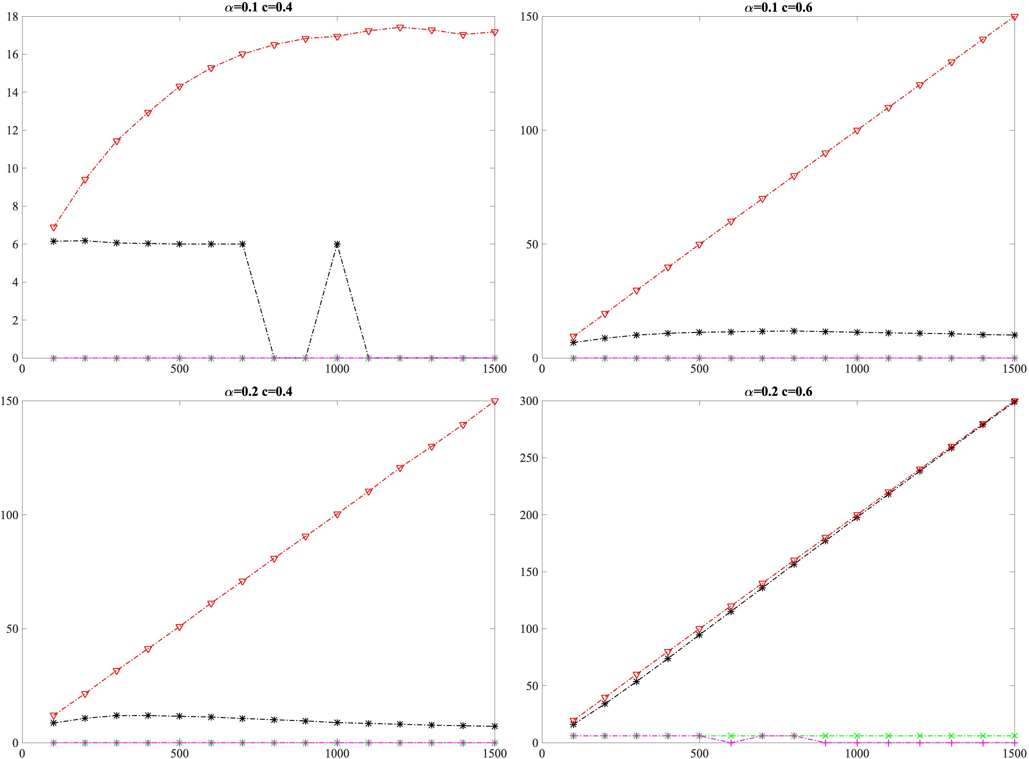
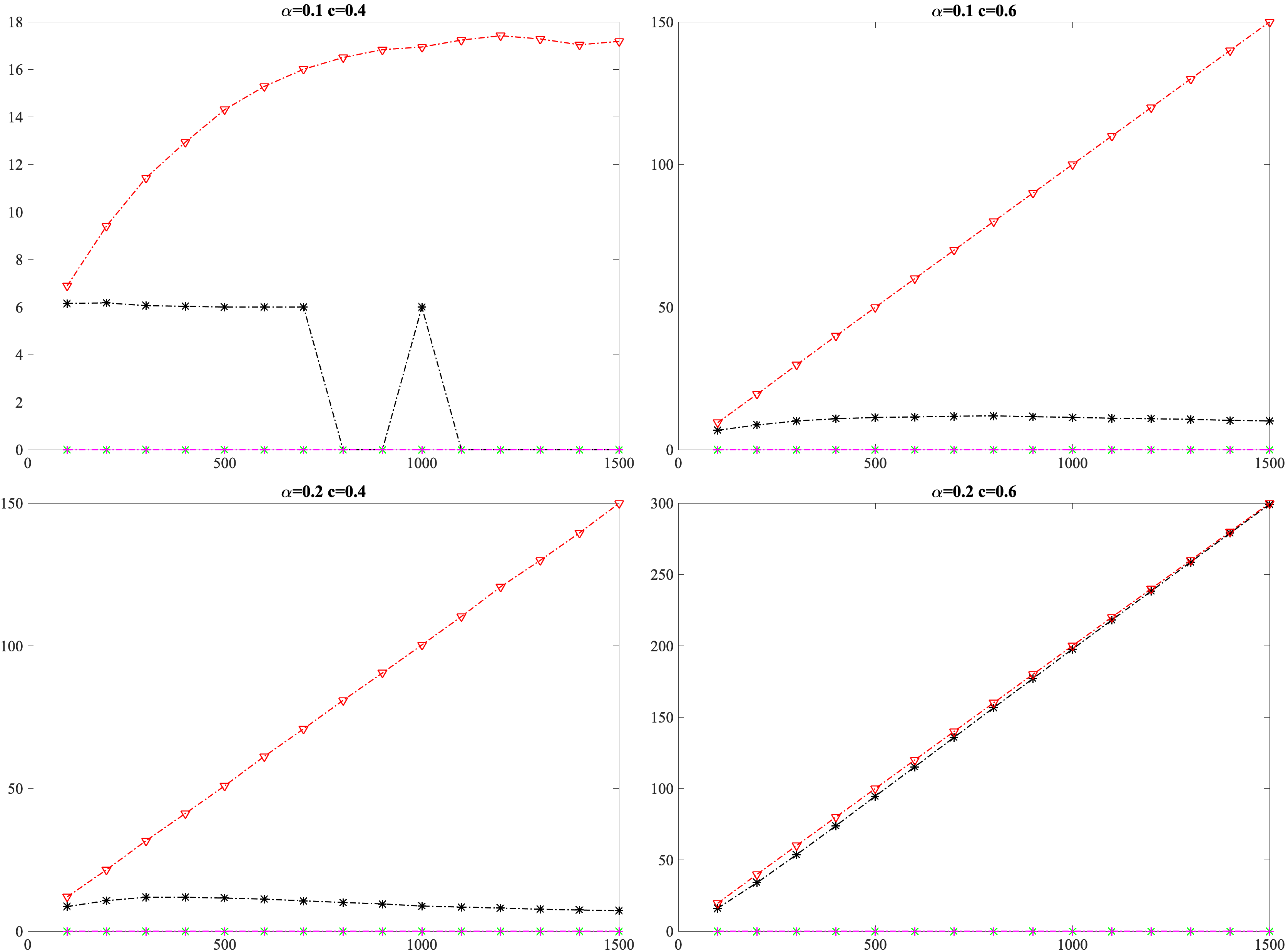
In this section, we present simulation results under a standardized $t$ distribution with three degrees of freedom and a standardized chi-square distribution with two degrees of freedom. Please see Figures 7-10. These results are similar to those of the normal distribution case. Thus, we guess that the consistency of these estimators depends on only the first two moments.

(a) Setting I

(b) Setting II

Figure 7: Selection percentages under the AIC, BIC and $C_{p}$ for Settings I and II with a standard $t_{3}$ distribution. The horizontal axes represent the sample size $n$, and the vertical axes represent selection percentage. Black solid circles, blue solid triangles, red solid squares, green solid hexagrams and magenta solid pentagrams denote the selection percentages of $\tilde{\bf j}_{A}={\bf j}_{*}$, $\tilde{\bf j}_{B}={\bf j}_{*}$, $\tilde{\bf j}_{C}={\bf j}_{*}$, $\breve{\bf j}_{A}={\bf j}_{*}$ and $\breve{\bf j}_{C}={\bf j}_{*}$, respectively. Correspondingly, black circles, blue triangles, red squares, green hexagrams and magenta pentagrams denote the selection percentages of $\tilde{\bf j}_{A}\in{\bf J}_{-}$, $\tilde{\bf j}_{B}\in{\bf J}_{-}$, $\tilde{\bf j}_{C}\in{\bf J}_{-}$, $\breve{\bf j}_{A}\in{\bf J}_{-}$ and $\breve{\bf j}_{C}\in{\bf J}_{-}$, respectively.

(a) Setting I

(b) Setting II

Figure 8: Overspecified model sizes of the AIC and $C_{p}$ for Settings I and II with a standard $t_{3}$ distribution. The horizontal axes represent the sample size $n$, and the vertical axes represent the model size. Black asterisks, red right-pointing triangles, green crosses and magenta plus signs denote the average sizes of $\tilde{\bf j}_{A}\in{\bf J}_{+}$, $\tilde{\bf j}_{C}\in{\bf J}_{+}$, $\breve{\bf j}_{A}\in{\bf J}_{+}$ and $\breve{\bf j}_{C}\in{\bf J}_{+}$, respectively. In this figure, we let $0/0=0$.

(a) Setting I

(b) Setting II

Figure 9: Selection percentages under the AIC, BIC and $C_{p}$ for Settings I and II with standard $\chi^{2}_{2}$ distribution. The horizontal axes represent the sample size $n$, and the vertical axes represent the selection percentages. Black solid circles, blue solid triangles, red solid squares, green solid hexagrams and magenta solid pentagrams denote the selection percentages of $\tilde{\bf j}_{A}={\bf j}_{*}$, $\tilde{\bf j}_{B}={\bf j}_{*}$, $\tilde{\bf j}_{C}={\bf j}_{*}$, $\breve{\bf j}_{A}={\bf j}_{*}$ and $\breve{\bf j}_{C}={\bf j}_{*}$, respectively. Correspondingly, black circles, blue triangles, red squares, green hexagrams and magenta pentagrams denote the selection percentages of $\tilde{\bf j}_{A}\in{\bf J}_{-}$, $\tilde{\bf j}_{B}\in{\bf J}_{-}$, $\tilde{\bf j}_{C}\in{\bf J}_{-}$, $\breve{\bf j}_{A}\in{\bf J}_{-}$ and $\breve{\bf j}_{C}\in{\bf J}_{-}$, respectively.

(a) Setting I

(b) Setting II

Figure 10: Overspecified model sizes of the AIC and $C_{p}$ for Settings I and II with a standard $chi_{2}^{2}$ distribution. The horizontal axes represent the sample size $n$, and the vertical axes represent the model size. Black asterisks, red right-pointing triangles, green crosses and magenta plus signs denote the average sizes of $\tilde{\bf j}_{A}\in{\bf J}_{+}$, $\tilde{\bf j}_{C}\in{\bf J}_{+}$, $\breve{\bf j}_{A}\in{\bf J}_{+}$ and $\breve{\bf j}_{C}\in{\bf J}_{+}$, respectively. In this figure we let $0/0=0$.

Appendix B Proof of Lemma 5.1

We now present the proof of Lemma 7.1. In the following, $C$ represents a generic constant whose value may vary from line to line.

Proof of Lemma 7.1.

According to the truncation approach of Bai et al. (2007), we can assume that the variables $\{e_{ij},i=1\dots n,j=1\dots p\}$ satisfy the following additional condition:

$$|e_{ij}|<C,\quad\mbox{for all $i,j$ and sufficiently large constant $C$}.$$

As the proof is very similar, we omit the details here. Let ${\mbox{\boldmath$\alpha$}}_{k1}$ be the $p-1$ subvector of ${\mbox{\boldmath$\alpha$}}_{1}$ with the $k$-th entry removed, and let $\alpha_{k1}$ be the $k$-th entry of ${\mbox{\boldmath$\alpha$}}_{1}$. Analogously, we can define ${\mbox{\boldmath$\alpha$}}_{k2}$ and $\alpha_{k2}$. Define ${\bf M}_{k}=\frac{1}{p}{\bf E}_{k}^{\prime}{\bf Q}_{{\bf j}_{-t}}{\bf E}_{k}-z{\bf I}_{p-1}$, where ${\bf E}_{k}$ is the $n\times(p-1)$ submatrix of ${\bf E}$ with the $k$-th column removed. Denote by ${\mathbb{E}}_{k}$ the conditional expectation given $\{{\bf e}_{1},\cdots,{\bf e}_{k}\}$ and by ${\mathbb{E}}_{0}$ the unconditional expectation, where ${\bf e}_{i}$ is the $n$-vector of the $i$-th column of ${\bf E}$. Then, by inverting the block matrix, we obtain

$${\mbox{\boldmath$\alpha$}}^{\prime}_{1}{\bf M}^{-1}{\mbox{\boldmath$\alpha$}}_{2}={\mbox{\boldmath$\alpha$}}_{k1}^{\prime}{\bf M}_{k}^{-1}{\mbox{\boldmath$\alpha$}}_{k2}+\frac{1}{\beta_{k}p^{2}}{\mbox{\boldmath$\alpha$}}_{k1}^{\prime}{\bf M}_{k}^{-1}{\bf E}_{k}^{\prime}{\bf Q}_{{\bf j}_{-t}}{\bf e}_{k}{\bf e}_{k}^{\prime}{\bf Q}_{{\bf j}_{-t}}{\bf E}_{k}{\bf M}_{k}^{-1}{\mbox{\boldmath$\alpha$}}_{k2}$$

$$-\frac{\alpha_{k2}}{\beta_{k}p}{\mbox{\boldmath$\alpha$}}_{k1}^{\prime}{\bf M}_{k}^{-1}{\bf E}_{k}^{\prime}{\bf Q}_{{\bf j}_{-t}}{\bf e}_{k}-\frac{\alpha_{k1}}{\beta_{k}p}{\bf e}_{k}^{\prime}{\bf Q}_{{\bf j}_{-t}}{\bf E}_{k}{\bf M}_{k}^{-1}{\mbox{\boldmath$\alpha$}}_{k2}+\frac{\alpha_{k1}\alpha_{k2}}{\beta_{k}},$$ (B.1)

where

$$\beta_{k} =\frac{1}{p}{\bf e}_{k}^{\prime}{\bf Q}_{{\bf j}_{-t}}{\bf e}_{k}-z-\frac{1}{p^{2}}{\bf e}_{k}^{\prime}{\bf Q}_{{\bf j}_{-t}}{\bf E}_{k}{\bf M}_{k}^{-1}{\bf E}_{k}^{\prime}{\bf Q}_{{\bf j}_{-t}}{\bf e}_{k}$$

$$=-z(1+\frac{1}{p}{\bf e}_{k}^{\prime}{\bf Q}_{{\bf j}_{-t}}\widehat{{\bf M}}_{k}^{-1}{\bf Q}_{{\bf j}_{-t}}{\bf e}_{k}).$$

The last equation is from the in-out-exchange formula (7.5) and

$$\widehat{{\bf M}}_{k}:=\frac{1}{p}{\bf Q}_{{\bf j}_{-t}}{\bf E}_{k}{\bf E}_{k}^{\prime}{\bf Q}_{{\bf j}_{-t}}-z{\bf I}_{n}.$$

Denote $\beta^{tr}_{k}=-z[1+\frac{1}{p}tr({\bf Q}_{{\bf j}_{-t}}\widehat{{\bf M}}_{k}^{-1})]$. It follows that

$$\frac{1}{\beta_{k}}=\frac{1}{\beta^{tr}_{k}}+\frac{\beta_{k}-\beta^{tr}_{k}}{p\beta_{k}\beta^{tr}_{k}}=\frac{1}{\beta^{tr}_{k}}+\frac{\xi_{k}}{\beta_{k}\beta^{tr}_{k}},$$ (B.2)

where $\xi_{k}=p^{-1}{\bf e}_{k}^{\prime}{\bf Q}_{{\bf j}_{-t}}\widehat{{\bf M}}_{k}^{-1}{\bf Q}_{{\bf j}_{-t}}{\bf e}_{k}-p^{-1}tr{\bf Q}_{{\bf j}_{-t}}\widehat{{\bf M}}_{k}^{-1}{\bf Q}_{{\bf j}_{-t}}$. It follows from (B.1) that

$${\mbox{\boldmath$\alpha$}}^{\prime}_{1}{\bf M}^{-1}{\mbox{\boldmath$\alpha$}}_{2}-{\mathbb{E}}{\mbox{\boldmath$\alpha$}}^{\prime}_{1}{\bf M}^{-1}{\mbox{\boldmath$\alpha$}}_{2}=\sum_{k=1}^{p}({\mathbb{E}}_{k}-{\mathbb{E}}_{k-1}){\mbox{\boldmath$\alpha$}}^{\prime}_{1}{\bf M}^{-1}{\mbox{\boldmath$\alpha$}}_{2}$$

$$= \sum_{k=1}^{p}({\mathbb{E}}_{k}-{\mathbb{E}}_{k-1})({\mbox{\boldmath$\alpha$}}^{\prime}_{1}{\bf M}^{-1}{\mbox{\boldmath$\alpha$}}_{2}-{\mbox{\boldmath$\alpha$}}_{k1}^{\prime}{\bf M}_{k}^{-1}{\mbox{\boldmath$\alpha$}}_{k2})$$

$$= \sum_{k=1}^{p}({\mathbb{E}}_{k}-{\mathbb{E}}_{k-1})({\cal M}_{1}-{\cal M}_{2}-{\cal M}_{3}+{\cal M}_{4}),$$

where

$${\cal M}_{1}=\frac{1}{\beta_{k}p^{2}}{\mbox{\boldmath$\alpha$}}_{k1}^{\prime}{\bf M}_{k}^{-1}{\bf E}_{k}^{\prime}{\bf Q}_{{\bf j}_{-t}}{\bf e}_{k}{\bf e}_{k}^{\prime}{\bf Q}_{{\bf j}_{-t}}{\bf E}_{k}{\bf M}_{k}^{-1}{\mbox{\boldmath$\alpha$}}_{k2},~{}{\cal M}_{2}=\frac{\alpha_{k2}}{\beta_{k}p}{\mbox{\boldmath$\alpha$}}_{k1}^{\prime}{\bf M}_{k}^{-1}{\bf E}_{k}^{\prime}{\bf Q}_{{\bf j}_{-t}}{\bf e}_{k}$$

$${\cal M}_{3}=\frac{\alpha_{k1}}{\beta_{k}p}{\bf e}_{k}^{\prime}{\bf Q}_{{\bf j}_{-t}}{\bf E}_{k}{\bf M}_{k}^{-1}{\mbox{\boldmath$\alpha$}}_{k2},~{}{\cal M}_{4}=\frac{\alpha_{k1}\alpha_{k2}}{\beta_{k}}.$$

Note that for any fixed $z\in\mathbb{C}^{+}$, we have

$$\min\{|\beta_{k}|,~{}|\beta^{tr}_{k}|,~{}\|{\bf M}_{k}\|,~{}\|\widehat{\bf M}_{k}\|\}\geq\Im z=v>0,$$

and $\|p^{-1/2}{\bf E}_{k}\|$ is almost surely bounded by a constant under assumption (A2) (see (Bai and Silverstein, 1998, 1999), for example). Thus, together with the condition that ${\mbox{\boldmath$\alpha$}}_{1}$ and ${\mbox{\boldmath$\alpha$}}_{2}$ are both bounded in Euclidean norm, we conclude that for $m\geq 1$

$${\mathbb{E}}|\xi_{k}|^{2m}\leq Cp^{-m}v^{-2m},$$ (B.3)

$${\mathbb{E}}|{\mbox{\boldmath$\alpha$}}_{k1}^{\prime}{\bf M}_{k}^{-1}{\bf E}_{k}^{\prime}{\bf Q}_{{\bf j}_{-t}},{\bf e}_{k}{\bf e}_{k}^{\prime}{\bf Q}_{{\bf j}_{-t}}{\bf E}_{k}{\bf M}_{k}^{-1}{\mbox{\boldmath$\alpha$}}_{k2}|^{m}\leq Cp^{m}v^{-2m}$$ (B.4)

$$\max\{{\mathbb{E}}|{\mbox{\boldmath$\alpha$}}_{k1}^{\prime}{\bf M}_{k}^{-1}{\bf E}_{k}^{\prime}{\bf Q}_{{\bf j}_{-t}}{\bf e}_{k}|^{2m},{\mathbb{E}}|{\bf e}_{k}^{\prime}{\bf Q}_{{\bf j}_{-t}}{\bf E}_{k}{\bf M}_{k}^{-1}{\mbox{\boldmath$\alpha$}}_{k2}|^{2m}\}\leq Cp^{m}v^{-2m}.$$ (B.5)

Here, we use the quadric form inequality shown in Lemma 2.7 of Bai and Silverstein (1998). Thus, by the Burkholder inequality (see Lemma 2.1 in (Bai and Silverstein, 1998)), we obtain

$${\mathbb{E}}\left|\sum_{k=1}^{p}({\mathbb{E}}_{k}-{\mathbb{E}}_{k-1}){\cal M}_{1}\right|^{4} \leq C{\mathbb{E}}\left(\sum_{k=1}^{p}{\mathbb{E}}_{k-1}|{\cal M}_{1}|^{2}\right)^{2}+C{\mathbb{E}}\sum_{k=1}^{p}|{\cal M}_{1}|^{4}$$

$$=O(p^{-2}).$$

Analogously, we also have

$${\mathbb{E}}\left|\sum_{k=1}^{p}({\mathbb{E}}_{k}-{\mathbb{E}}_{k-1}){\cal M}_{2}\right|^{4}=O(p^{-2})\mbox{~{}and~{}}{\mathbb{E}}\left|\sum_{k=1}^{p}({\mathbb{E}}_{k}-{\mathbb{E}}_{k-1}){\cal M}_{3}\right|^{4}=O(p^{-2}).$$

For ${\cal M}_{4}$, by (B.3), (B.2) and the Burkholder inequality, we obtain

$${\mathbb{E}}\left|\sum_{k=1}^{p}({\mathbb{E}}_{k}-{\mathbb{E}}_{k-1}){\cal M}_{4}\right|^{4}={\mathbb{E}}\left|\sum_{k=1}^{p}({\mathbb{E}}_{k}-{\mathbb{E}}_{k-1})\frac{\xi_{k}}{\beta_{k}\beta^{tr}_{k}}\right|^{4}=O(p^{-2}),$$

which finally implies

$${\mathbb{E}}|{\mbox{\boldmath$\alpha$}}^{\prime}_{1}{\bf M}^{-1}{\mbox{\boldmath$\alpha$}}_{2}-{\mathbb{E}}{\mbox{\boldmath$\alpha$}}^{\prime}_{1}{\bf M}^{-1}{\mbox{\boldmath$\alpha$}}_{2}|^{4}=O(p^{-2}).$$

Therefore, by the Borel-Cantelli lemma, we have that

$${\mbox{\boldmath$\alpha$}}^{\prime}_{1}{\bf M}^{-1}{\mbox{\boldmath$\alpha$}}_{2}-{\mathbb{E}}{\mbox{\boldmath$\alpha$}}^{\prime}_{1}{\bf M}^{-1}{\mbox{\boldmath$\alpha$}}_{2}\stackrel{{\scriptstyle a.s.}}{{\to}}0.$$ (B.6)

Because the entry distributions of ${\bf E}$ are identical, we know that the diagonal elements of ${\mathbb{E}}{\bf M}^{-1}$ are the same, denoted as $a_{n}(z)$ in the following. The off-diagonal elements are also the same, denoted as $b_{n}(z)$. From (B.1), (B.2) and (B.3), we have

$$a_{n}(z) ={\mathbb{E}}\frac{1}{\beta_{1}}={\mathbb{E}}\frac{1}{\beta^{tr}_{1}}+o(1).$$ (B.7)

Let $\lambda_{1}\geq\cdots\geq\lambda_{n}\geq 0$ be the eigenvalues of $p^{-1}{\bf Q}_{{\bf j}_{-t}}{\bf E}_{1}{\bf E}_{1}^{\prime}{\bf Q}_{{\bf j}_{-t}}$ whose corresponding eigenvectors are denoted by ${\bf v}_{1},\cdots,{\bf v}_{n}$. Note that the rank of ${\bf Q}_{{\bf j}_{-t}}$ is $n-k_{{\bf j}_{-t}}$, the dimension of the null space of ${\bf Q}_{{\bf j}_{-t}}$ is $k_{{\bf j}_{-t}}$, and the null space of $p^{-1}{\bf Q}_{{\bf j}_{-t}}{\bf E}_{1}{\bf E}_{1}^{\prime}{\bf Q}_{{\bf j}_{-t}}$ is not smaller than that of ${\bf Q}_{{\bf j}_{-t}}$. Thus, we may select the last $k_{{\bf j}_{-t}}$ eigenvectors from the null space of ${\bf Q}_{{\bf j}_{-t}}$, that is, we may assume that ${\bf Q}_{{\bf j}_{-t}}{\bf v}_{i}=0$, $i=n-k_{{\bf j}_{-t}}+1,\cdots,n$. Therefore, the matrix $\widehat{{\bf M}}_{1}^{-1}{\bf Q}_{{\bf j}_{-t}}$ has $k_{{\bf j}_{-t}}$-fold eigenvalue $0$. By contrast, for all $i=1,\cdots,n-k_{{\bf j}_{-t}}$, ${\bf Q}_{{\bf j}_{-t}}{\bf v}_{i}\neq 0$ and ${\bf Q}_{{\bf j}_{-t}}{\bf v}_{i}$ is also an eigenvector of $p^{-1}{\bf Q}_{{\bf j}_{-t}}{\bf E}_{1}{\bf E}_{1}^{\prime}{\bf Q}_{{\bf j}_{-t}}$ corresponding to $\lambda_{i}$, that is,

$$p^{-1}{\bf Q}_{{\bf j}_{-t}}{\bf E}_{1}{\bf E}_{1}^{\prime}{\bf Q}_{{\bf j}_{-t}}{\bf v}_{i}=\lambda_{i}{\bf Q}_{{\bf j}_{-t}}{\bf v}_{i},$$

which is equivalent to

$$(p^{-1}{\bf Q}_{{\bf j}_{-t}}{\bf E}_{1}{\bf E}_{1}^{\prime}{\bf Q}_{{\bf j}_{-t}}-z{\bf I}_{n})^{-1}{\bf Q}_{{\bf j}_{-t}}{\bf v}_{i}=(\lambda_{i}-z)^{-1}{\bf Q}_{{\bf j}_{-t}}{\bf v}_{i}.$$

Thus, $(\lambda_{i}-z)^{-1}$ is a nonzero eigenvalue of $\widehat{{\bf M}}_{1}^{-1}{\bf Q}_{{\bf j}_{-t}}$. Therefore,

$$\frac{1}{p}{\rm tr}\widehat{{\bf M}}_{1}^{-1}{\bf Q}_{{\bf j}_{-t}}=\frac{1}{p}\sum_{i=1}^{n-k_{{\bf j}_{-t}}}\frac{1}{\lambda_{i}-z}=\frac{1}{p}\sum_{i=1}^{n}\frac{1}{\lambda_{i}-z}+\frac{k_{{\bf j}_{-t}}}{pz}=\frac{1}{p}tr\widehat{{\bf M}}_{1}^{-1}+\frac{k_{{\bf j}_{-t}}}{pz}.$$

Since the spectra of $p^{-1}{\bf Q}_{{\bf j}_{-t}}{\bf E}_{1}{\bf E}_{1}^{\prime}{\bf Q}_{{\bf j}_{-t}}$ and $p^{-1}{\bf E}_{1}^{\prime}{\bf Q}_{{\bf j}_{-t}}{\bf E}_{1}$ differ by $|n-p-1|$ zero eigenvalues, it follows that

$${\mathbb{E}}\frac{1}{p}tr\widehat{{\bf M}}_{1}^{-1}={\mathbb{E}}{\frac{1}{p}tr{{\bf M}}_{1}^{-1}+\frac{1-n/p}{z}}\to\underline{s}_{t}(z)+\frac{c-1}{cz}.$$

Together with (B.7) and the last equation, we obtain

$$a_{n}(z)\to-\frac{1}{z(1+\underline{s}_{t}(z)+\frac{c-1+\alpha_{m-t}}{cz})}.$$ (B.8)

Here, $\alpha_{m-t}=\lim k_{{\bf j}_{-t}}/n.$

Furthermore, from the inverse matrix formula, we obtain

$$b_{n}(z) = {\mathbb{E}}\left(\frac{{\bf u}_{1}^{\prime}{\bf M}_{1}^{-1}{\bf E}_{1}^{\prime}{\bf Q}_{{\bf j}_{-t}}{\bf e}_{1}}{p\beta_{1}}\right),$$

where ${\bf u}_{1}=(1,0,\cdots,0)^{\prime}$ is a $(p-1)$-dimensional vector, and ${\bf e}_{1}$ is the first column of ${\bf E}$. Because ${\bf e}_{1}$ is independent of ${\bf E}_{1}$, by the Cauchy-Schwarz inequality and equation (B.2), we have

$$|b_{n}(z)| =\left|{\mathbb{E}}\left(\frac{{\bf u}_{1}^{\prime}{\bf M}_{1}^{-1}{\bf E}_{1}^{\prime}{\bf Q}_{{\bf j}_{-t}}{\bf e}_{1}\xi_{1}}{p\beta_{1}\beta_{1}^{tr}}\right)\right|=O(p^{-1}).$$ (B.9)

Therefore, by combining (B.6)-(B.9) and the $C_{r}$ inequality, the proof of (7.6) is complete.

For the proof of (7.7), using the inverse of block matrix again, we obtain

$${\mbox{\boldmath$\alpha$}}^{\prime}_{1}{\bf M}^{-1}{\bf E}^{\prime}{\mbox{\boldmath$\alpha$}}_{2}={\mbox{\boldmath$\alpha$}}_{k1}^{\prime}{\bf M}_{k}^{-1}{\bf E}_{k}^{\prime}{\mbox{\boldmath$\alpha$}}_{2}+\frac{1}{\beta_{k}p^{2}}{\mbox{\boldmath$\alpha$}}_{k1}^{\prime}{\bf M}_{k}^{-1}{\bf E}_{k}^{\prime}{\bf Q}_{{\bf j}_{-t}}{\bf e}_{k}{\bf e}_{k}^{\prime}{\bf Q}_{{\bf j}_{-t}}{\bf E}_{k}{\bf M}_{k}^{-1}{\bf E}_{k}^{\prime}{\mbox{\boldmath$\alpha$}}_{2}$$

$$-\frac{\alpha_{k2}}{\beta_{k}p}{\mbox{\boldmath$\alpha$}}_{k1}^{\prime}{\bf M}_{k}^{-1}{\bf E}_{k}^{\prime}{\bf Q}_{{\bf j}_{-t}}{\bf e}_{k}-\frac{\alpha_{k1}}{\beta_{k}p}{\bf e}_{k}^{\prime}{\bf Q}_{{\bf j}_{-t}}{\bf E}_{k}{\bf M}_{k}^{-1}{\bf E}_{k}^{\prime}{\mbox{\boldmath$\alpha$}}_{2}+\frac{\alpha_{k1}{\bf e}_{k}^{\prime}{\mbox{\boldmath$\alpha$}}_{2}}{\beta_{k}}.$$

By means of the same procedure used in the proof of (7.6), we can obtain that, almost surely,

$$\frac{1}{\sqrt{p}}{\mbox{\boldmath$\alpha$}}_{1}^{\prime}{\bf M}^{-1}{\bf E}^{\prime}{\mbox{\boldmath$\alpha$}}_{2}-\frac{1}{\sqrt{p}}{\mathbb{E}}{\mbox{\boldmath$\alpha$}}_{1}^{\prime}{\bf M}^{-1}{\bf E}^{\prime}{\mbox{\boldmath$\alpha$}}_{2}\to 0.$$

Next, we show that $\frac{1}{\sqrt{p}}{\mathbb{E}}{\mbox{\boldmath$\alpha$}}_{1}^{\prime}{\bf M}^{-1}{\bf E}^{\prime}{\mbox{\boldmath$\alpha$}}_{2}=o(1).$ Write ${\bf M}^{-1}=(M^{ij})$. Then, we have

$$\frac{1}{\sqrt{p}}{\mathbb{E}}{\mbox{\boldmath$\alpha$}}_{1}^{\prime}{\bf M}^{-1}{\bf E}^{\prime}{\mbox{\boldmath$\alpha$}}_{2}=\frac{1}{\sqrt{p}}\sum_{ij}\alpha_{i1}{\mathbb{E}}M^{ij}{\bf e}_{j}^{\prime}{\mbox{\boldmath$\alpha$}}_{2}$$

$$= \frac{1}{\sqrt{p}}\sum_{i=1}^{p}\alpha_{i1}\left({\mathbb{E}}M^{11}{\bf e}_{1}^{\prime}{\mbox{\boldmath$\alpha$}}_{2}+(p-1){\mathbb{E}}M^{12}{\bf e}_{2}^{\prime}{\mbox{\boldmath$\alpha$}}_{2}\right)$$

$$= \frac{1}{\sqrt{p}}\sum_{i=1}^{p}\alpha_{i1}\left({\mathbb{E}}\frac{{\bf e}_{1}^{\prime}{\mbox{\boldmath$\alpha$}}_{2}}{\beta_{1}}-(p-1){\mathbb{E}}\frac{{\bf u}_{1}^{\prime}{\bf M}_{1}^{-1}{\bf E}_{1}^{\prime}{\bf Q}_{{\bf j}_{-t}}{\bf e}_{1}{\bf e}_{2}^{\prime}{\mbox{\boldmath$\alpha$}}_{2}}{p\beta_{1}}\right)$$

$$= \frac{1}{\sqrt{p}}\sum_{i=1}^{p}\alpha_{i1}\left({\mathbb{E}}\frac{\xi_{1}{\bf e}_{1}^{\prime}{\mbox{\boldmath$\alpha$}}_{2}}{\beta_{1}\beta_{1}^{tr}}-(p-1){\mathbb{E}}\frac{{\bf u}_{1}^{\prime}{\bf M}_{1}^{-1}{\bf E}_{1}^{\prime}{\bf Q}_{{\bf j}_{-t}}{\bf e}_{1}{\bf e}_{2}^{\prime}{\mbox{\boldmath$\alpha$}}_{2}\xi_{1}}{p\beta_{1}\beta_{1}^{tr}}\right)$$

$$= \frac{1}{p^{3/2}}\sum_{i=1}^{p}\alpha_{i1}\sum_{j=1}^{n}{\mathbb{E}}\frac{e_{j1}^{3}({\bf Q}_{{\bf j}_{-t}}\widehat{{\bf M}}_{1}^{-1}{\bf Q}_{{\bf j}_{-t}})_{jj}\alpha_{j1}}{(\beta_{1}^{tr})^{2}}$$

$$-\frac{1}{\sqrt{p}}\sum_{i=1}^{p}\alpha_{i1}{\mathbb{E}}\frac{{\bf u}_{1}^{\prime}{\bf M}_{1}^{-1}{\bf E}_{1}^{\prime}{\bf Q}_{{\bf j}_{-t}}{\bf e}_{1}{\bf e}_{2}^{\prime}{\mbox{\boldmath$\alpha$}}_{2}\xi_{1}}{(\beta_{1}^{tr})^{2}}+o(1)$$

$$= o(1),$$

which completes the proof of (7.7). In the above equation, we use (B.3), the Cauchy-Schwarz inequality, the $C_{r}$ inequality and the facts that

$$\sum_{i=1}^{p}|\alpha_{i1}|\leq\left(p\sum_{i=1}^{p}|\alpha_{i1}^{2}|\right)^{1/2}=O(\sqrt{p})$$

and

$$\left|{\mathbb{E}}\frac{{\bf u}_{2}^{\prime}{\bf M}_{1}^{-1}{\bf E}_{1}^{\prime}{\bf Q}_{{\bf j}_{-t}}{\bf e}_{1}{\bf e}_{2}^{\prime}{\mbox{\boldmath$\alpha$}}_{2}\xi_{1}}{\sqrt{p}\beta_{1}\beta_{1}^{tr}}\right|$$

$$\leq \left|{\mathbb{E}}\frac{{\bf u}_{2}^{\prime}{\bf M}_{1}^{-1}{\bf E}_{1}^{\prime}{\bf Q}_{{\bf j}_{-t}}{\bf e}_{1}{\bf e}_{2}^{\prime}{\mbox{\boldmath$\alpha$}}_{2}\xi_{1}}{\sqrt{p}(\beta_{1}^{tr})^{2}}\right|+{\mathbb{E}}\left|\frac{({\bf u}_{2}^{\prime}{\bf M}_{1}^{-1}{\bf E}_{1}^{\prime}{\bf Q}_{{\bf j}_{-t}}{\bf e}_{1}{\bf e}_{2}^{\prime}{\mbox{\boldmath$\alpha$}}_{2})\xi_{1}^{2}}{\sqrt{p}(\beta_{1}^{tr})^{2}\beta_{1}}\right|$$

$$= O(p^{-1/2}).$$

Next, we give the proof of (7.1). The random part is analogous to the proof of (7.6), which is, almost surely

$$\frac{1}{{p}}{\mbox{\boldmath$\alpha$}}_{1}^{\prime}{\bf E}{\bf M}^{-1}{\bf E}^{\prime}{\mbox{\boldmath$\alpha$}}_{2}-\frac{1}{{p}}{\mathbb{E}}{\mbox{\boldmath$\alpha$}}_{1}^{\prime}{\bf E}{\bf M}^{-1}{\bf E}^{\prime}{\mbox{\boldmath$\alpha$}}_{2}\to 0,$$

and we omit the details here. Next, we focus on the nonrandom part. By means of the inverse of the block matrix, we have

$$\frac{1}{{p}}{\mathbb{E}}{\mbox{\boldmath$\alpha$}}_{1}^{\prime}{\bf E}{\bf M}^{-1}{\bf E}^{\prime}{\mbox{\boldmath$\alpha$}}_{2}=\frac{1}{{p}}\sum_{ij}{\mathbb{E}}{\mbox{\boldmath$\alpha$}}_{1}^{\prime}{\bf e}_{i}M^{ij}{\bf e}_{j}^{\prime}{\mbox{\boldmath$\alpha$}}_{2}$$

$$= {\mathbb{E}}{\mbox{\boldmath$\alpha$}}_{1}^{\prime}{\bf e}_{1}M^{11}{\bf e}_{1}^{\prime}{\mbox{\boldmath$\alpha$}}_{2}+(p-1){\mathbb{E}}{\mbox{\boldmath$\alpha$}}_{1}^{\prime}{\bf e}_{1}M^{12}{\bf e}_{2}^{\prime}{\mbox{\boldmath$\alpha$}}_{2})$$

$$= {\mathbb{E}}\frac{{\mbox{\boldmath$\alpha$}}_{1}^{\prime}{\bf e}_{1}{\bf e}_{1}^{\prime}{\mbox{\boldmath$\alpha$}}_{2}}{\beta_{1}}-(p-1){\mathbb{E}}\frac{{\mbox{\boldmath$\alpha$}}_{1}^{\prime}{\bf e}_{1}{\bf u}_{1}^{\prime}{\bf M}_{1}^{-1}{\bf E}_{1}^{\prime}{\bf Q}_{{\bf j}_{-t}}{\bf e}_{1}{\bf e}_{2}^{\prime}{\mbox{\boldmath$\alpha$}}_{2}}{p\beta_{1}}$$

$$= {\mathbb{E}}\frac{{\mbox{\boldmath$\alpha$}}_{1}^{\prime}{\mbox{\boldmath$\alpha$}}_{2}}{\beta_{1}^{tr}}-(p-1){\mathbb{E}}\frac{{\bf u}_{1}^{\prime}{\bf M}_{1}^{-1}{\bf E}_{1}^{\prime}{\bf Q}_{{\bf j}_{-t}}{\mbox{\boldmath$\alpha$}}_{1}{\bf e}_{2}^{\prime}{\mbox{\boldmath$\alpha$}}_{2}}{p\beta_{1}^{tr}}$$

$$+{\mathbb{E}}\frac{\xi_{1}{\mbox{\boldmath$\alpha$}}_{1}^{\prime}{\bf e}_{1}{\bf e}_{1}^{\prime}{\mbox{\boldmath$\alpha$}}_{2}}{\beta_{1}\beta_{1}^{tr}}-(p-1){\mathbb{E}}\frac{{\mbox{\boldmath$\alpha$}}_{1}^{\prime}{\bf e}_{1}{\bf u}_{1}^{\prime}{\bf M}_{1}^{-1}{\bf E}_{1}^{\prime}{\bf Q}_{{\bf j}_{-t}}{\bf e}_{1}{\bf e}_{2}^{\prime}{\mbox{\boldmath$\alpha$}}_{2}\xi_{1}}{p\beta_{1}\beta_{1}^{tr}}.$$

It follows from (B.8) that

$${\mathbb{E}}\frac{{\mbox{\boldmath$\alpha$}}_{1}^{\prime}{\mbox{\boldmath$\alpha$}}_{2}}{\beta_{1}^{tr}}\to-\frac{{\mbox{\boldmath$\alpha$}}_{1}^{\prime}{\mbox{\boldmath$\alpha$}}_{2}}{z(1+\underline{s}_{t}(z)+\frac{c-1+\alpha_{m-t}}{cz})}.$$ (B.10)

Using the inverse of block matrix again, we obtain

$${\mathbb{E}}{\bf u}_{1}^{\prime}{\bf M}_{1}^{-1}{\bf E}_{1}^{\prime}{\bf Q}_{{\bf j}_{-t}}{\mbox{\boldmath$\alpha$}}_{1}{\bf e}_{2}^{\prime}{\mbox{\boldmath$\alpha$}}_{2}$$

$$={\mathbb{E}}\frac{{\bf e}_{2}^{\prime}{\bf Q}_{{\bf j}_{-t}}{\mbox{\boldmath$\alpha$}}_{1}{\bf e}_{2}^{\prime}{\mbox{\boldmath$\alpha$}}_{2}}{\beta_{12}}-{\mathbb{E}}\frac{1}{\beta_{12}p}{\bf e}_{2}^{\prime}{\bf Q}_{{\bf j}_{-t}}{\bf E}_{12}{\bf M}_{12}^{-1}{\bf E}_{12}^{\prime}{\bf Q}_{{\bf j}_{-t}}{\mbox{\boldmath$\alpha$}}_{1}{\bf e}_{2}^{\prime}{\mbox{\boldmath$\alpha$}}_{2},$$

which together with (B.2), (B.3) and in-out-exchange foumula (7.5) implies

$${\mathbb{E}}\frac{{\bf u}_{1}^{\prime}{\bf M}_{1}^{-1}{\bf E}_{1}^{\prime}{\bf Q}_{{\bf j}_{-t}}{\mbox{\boldmath$\alpha$}}_{1}{\bf e}_{2}^{\prime}{\mbox{\boldmath$\alpha$}}_{2}}{\beta_{1}^{tr}}$$

$$= {\mathbb{E}}\frac{{\mbox{\boldmath$\alpha$}}_{1}^{\prime}{\bf Q}_{{\bf j}_{-t}}{\mbox{\boldmath$\alpha$}}_{2}}{(\beta_{12}^{tr})^{2}}-{\mathbb{E}}\frac{{\mbox{\boldmath$\alpha$}}_{1}{\bf Q}_{{\bf j}_{-t}}{\bf E}_{12}{\bf M}_{12}^{-1}{\bf E}_{12}^{\prime}{\bf Q}_{{\bf j}_{-t}}{\mbox{\boldmath$\alpha$}}_{2}}{p(\beta_{12}^{tr})^{2}}+o(1)$$

$$= -{\mathbb{E}}\frac{z{\mbox{\boldmath$\alpha$}}_{1}{\bf Q}_{{\bf j}_{-t}}\widehat{\bf M}_{12}^{-1}{\bf Q}_{{\bf j}_{-t}}{\mbox{\boldmath$\alpha$}}_{2}}{(\beta_{12}^{tr})^{2}}+o(1).$$

Here, ${\bf E}_{12}$ is the $n\times(p-2)$ submatrix of ${\bf E}$ with the first and second columns removed. $\beta_{12}$, $\beta_{12}^{tr}$, ${\bf M}_{12}^{-1}$ and $\widehat{\bf M}_{12}^{-1}$ are denoted analogously. Note that ${\mathbb{E}}\frac{\xi_{1}{\mbox{\boldmath$\alpha$}}_{1}^{\prime}{\bf e}_{1}{\bf e}_{1}^{\prime}{\mbox{\boldmath$\alpha$}}_{2}}{\beta_{1}\beta_{1}^{tr}}$ and ${\mathbb{E}}\frac{{\mbox{\boldmath$\alpha$}}_{1}^{\prime}{\bf e}_{1}{\bf u}_{1}^{\prime}{\bf M}_{1}^{-1}{\bf E}_{1}^{\prime}{\bf Q}_{{\bf j}_{-t}}{\bf e}_{1}{\bf e}_{2}^{\prime}{\mbox{\boldmath$\alpha$}}_{2}\xi_{1}}{\beta_{1}\beta_{1}^{tr}}$ are both $o(1)$ because of (B.2) and (B.3). Similar to (5.9) in Bai et al. (2007), we have

$${\mathbb{E}}{\mbox{\boldmath$\alpha$}}_{1}^{\prime}{\bf Q}_{{\bf j}_{-t}}\widehat{\bf M}_{12}^{-1}{\bf Q}_{{\bf j}_{-t}}{\mbox{\boldmath$\alpha$}}_{2}-{\mbox{\boldmath$\alpha$}}_{1}{\bf Q}_{{\bf j}_{-t}}(-z\underline{s}_{t}(z){\bf Q}_{{\bf j}_{-t}}-z{\bf I})^{-1}{\bf Q}_{{\bf j}_{-t}}{\mbox{\boldmath$\alpha$}}_{2}\to 0.$$

As ${\mbox{\boldmath$\alpha$}}_{1}^{\prime}{\bf Q}_{{\bf j}_{-t}}$ and ${\bf Q}_{{\bf j}_{-t}}{\mbox{\boldmath$\alpha$}}_{2}$ are both eigenvectors of ${\bf Q}_{{\bf j}_{-t}}$, we obtain

$${\mbox{\boldmath$\alpha$}}_{1}{\bf Q}_{{\bf j}_{-t}}(z\underline{s}_{t}(z){\bf Q}_{{\bf j}_{-t}}+z{\bf I})^{-1}{\bf Q}_{{\bf j}_{-t}}{\mbox{\boldmath$\alpha$}}_{2}=\frac{{\mbox{\boldmath$\alpha$}}_{1}{\bf Q}_{{\bf j}_{-t}}{\mbox{\boldmath$\alpha$}}_{2}}{z\underline{s}_{t}(z)+z},$$

which together with (B.10) and the fact that

$${\mathbb{E}}\beta_{1}^{-1}-{\mathbb{E}}\beta_{12}^{-1}\to 0,$$

completes the proof of (7.1). Thus, the proof of this lemma is complete. ∎

References

- Akaike (1973) H. Akaike. Information theory and an extension of the maximum likehood principle. In Second International Symposium on Information Theory, pages 267–281. 1973. ISBN 0012-9682. 10.2307/2938260.
- Anzanello and Fogliatto (2014) M. J. Anzanello and F. S. Fogliatto. A review of recent variable selection methods in industrial and chemometrics applications. European J. of Industrial Engineering, 8(5):619, 2014.
- Bai et al. (2018) Z. D. Bai, K. P. Choi, and Y. Fujikoshi. Consistency of AIC and BIC in estimating the number of significant components in high-dimensional principal component analysis. The Annals of Statistics, 46(3):1050–1076, jun 2018.
- Bai and Silverstein (1998) Z. D. Bai and J. W. Silverstein. No eigenvalues outside the support of the limiting spectral distribution of large-dimensional sample covariance matrices. The Annals of Probability, 26(1):316–345, Jan. 1998.
- Bai and Silverstein (1999) Z. D. Bai and J. W. Silverstein. Exact separation of eigenvalues of large dimensional sample covariance matrices. The Annals of Probability, 27(3):1536–1555, 1999.
- Bai and Silverstein (2010) Z. D. Bai and J. W. Silverstein. Spectral analysis of large dimensional random matrices. Second Edition. Springer Verlag, 2010.
- Bai et al. (2007) Z. D. Bai, B. Q. Miao, and G. M. Pan. On asymptotics of eigenvectors of large sample covariance matrix. The Annals of Probability, 35(4):1532–1572, July 2007.
- Bao et al. (2018) Z. Bao, J. Hu, G. Pan, and W. Zhou. Canonical correlation coefficients of high-dimensional Gaussian vectors: finite rank case. The Annals of Statistics (to appear), 2018.
- Barnett and Lewis (1994) V. Barnett and T. Lewis. Outliers in Statistical Data. Wiley, 3rd ed edition, 1994.
- Blei et al. (2017) D. M. Blei, A. Kucukelbir, and J. D. McAuliffe. Variational Inference: A Review for Statisticians. Journal of the American Statistical Association, 112(518):859–877, 2017.
- Bozdogan (1987) H. Bozdogan. Model selection and Akaike’s Information Criterion (AIC): The general theory and its analytical extensions. Psychometrika, 52(3):345–370, sep 1987.
- Breiman and Friedman (1997) L. Breiman and J. H. Friedman. Predicting Multivariate Responses in Multiple Linear Regression. Journal of the Royal Statistical Society: Series B (Statistical Methodology), 59(1):3–54, 1997.
- Chen and Huang (2012) L. Chen and J. Z. Huang. Sparse Reduced-Rank Regression for Simultaneous Dimension Reduction and Variable Selection. Journal of the American Statistical Association, 107(500):1533–1545, Dec. 2012. ISSN 0162-1459.
- Chen et al. (2011) L. Chen, D. Paul, R. Prentice, and P. Wang. A regularized Hotelling’s test for pathway analysis in proteomic studies. Journal of the American Statistical Association, 106(496):1345–1360, 2011.
- Chun and Keleş (2010) H. Chun and S. Keleş. Sparse Partial Least Squares Regression for Simultaneous Dimension Reduction and Variable Selection. Journal of the Royal Statistical Society. Series B (Statistical Methodology), 72(1):3–25, 2010.
- Enomoto et al. (2015) R. Enomoto, T. Sakurai, and Y. Fujikoshi. Consistency properties of AIC, BIC, Cp and their modifications in the growth curve model under a large-(q,n) framework. SUT Journal of Mathematics, 51(1):59–81, 2015.
- Fan and Lv (2008) J. Fan and J. Lv. Sure independence screening for ultrahigh dimensional feature space. Journal of the Royal Statistical Society: Series B (Statistical Methodology), 70(5):849–911, 2008.
- Fan and Lv (2010) J. Fan and J. Lv. A selective overview of variable selection in high dimensional feature space. Statistica Sinica, 20:101–148, 2010.
- Fujikoshi (1983) Y. Fujikoshi. A criterion for variable selection in multiple discriminant analysis. Hiroshima Mathematical Journal, 13(1):203–214, 1983.
- Fujikoshi (1985) Y. Fujikoshi. Selection of variables in two-group discriminant analysis by error rate and Akaike’s information criteria. Journal of Multivariate Analysis, 17(1):27–37, aug 1985.
- Fujikoshi and Sakurai (2016a) Y. Fujikoshi and T. Sakurai. High-dimensional consistency of rank estimation criteria in multivariate linear model. Journal of Multivariate Analysis, 149:199–212, 2016a.
- Fujikoshi and Sakurai (2016b) Y. Fujikoshi and T. Sakurai. Some Properties of Estimation Criteria for Dimensionality in Principal Component Analysis. American Journal of Mathematical and Management Sciences, 35(2):133–142, 2016b.
- Fujikoshi and Sakurai (2018) Y. Fujikoshi and T. Sakurai. Consistency of Test-based Criterion for Selection of Variables in High-dimensional Two Group-Discriminant Analysis. Japanese Journal of Statistics and Data Science (to appear), 2018.
- Fujikoshi and Satoh (1997) Y. Fujikoshi and K. Satoh. Modified AIC and in multivariate linear regression. Biometrika, 84(3):707–716, 1997.
- Fujikoshi and Veitch (1979) Y. Fujikoshi and L. G. Veitch. Estimation of dimensionality in canonical correlation analysis. Biometrika, 66(2):345–351, 1979.
- Fujikoshi et al. (2013) Y. Fujikoshi, R. Enomoto, and T. Sakurai. High-dimensional in the growth curve model. Journal of Multivariate Analysis, 122:239–250, 2013.
- Fujikoshi et al. (2014) Y. Fujikoshi, T. Sakurai, and H. Yanagihara. Consistency of high-dimensional AIC-type and -type criteria in multivariate linear regression. Journal of Multivariate Analysis, 123:184–200, 2014.
- Heinze et al. (2018) G. Heinze, C. Wallisch, and D. Dunkler. Variable selection - A review and recommendations for the practicing statistician. Biometrical Journal, 60(3):431–449, may 2018.
- Kong et al. (2017) Y. Kong, D. Li, Y. Fan, and J. Lv. Interaction pursuit in high-dimensional multi-response regression via distance correlation. The Annals of Statistics, 45(2):897–922, 2017.
- Li et al. (2012) R. Li, W. Zhong, and L. Zhu. Feature Screening via Distance Correlation Learning. Journal of the American Statistical Association, 107(499):1129–1139, 2012.
- Li et al. (2015) Y. Li, B. Nan, and J. Zhu. Multivariate sparse group lasso for the multivariate multiple linear regression with an arbitrary group structure. Biometrics, 71(2):354–363, jun 2015.
- Mallows (1973) C. L. Mallows. Some Comments on Cp. Technometrics, 15(4):661, 1973.
- Nishii et al. (1988) R. Nishii, Z. Bai, and P. R. Krishnaiah. Strong consistency of the information criterion for model selection in multivariate analysis. Hiroshima Mathematical Journal, 18(3):451–462, 1988.
- Schwarz (1978) G. Schwarz. Estimating the dimension of a model. The Annals of Statistics, 6(2):461–464, 1978.
- Skagerberg et al. (1992) B. Skagerberg, J. F. MacGregor, and C. Kiparissides. Multivariate data analysis applied to low-density polyethylene reactors. Chemometrics and Intelligent Laboratory Systems, 14(1):341–356, Apr. 1992.
- Silverstein and Choi (1995) J. W. Silverstein and S. I. Choi. Analysis of the limiting spectral distribution of large dimensional random matrices. Journal of Multivariate Analysis, 54(2):295–309, 1995.
- Similä and Tikka (2007) T. Similä and J. Tikka. Input selection and shrinkage in multiresponse linear regression. Computational Statistics & Data Analysis, 52(1):406–422, 2007.
- Sparks et al. (1983) R. Sparks, D. Coutsourides, and L. Troskie. The multivariate Cp. Communications in Statistics - Theory and Methods, 12(15):1775–1793, jan 1983.
- Spellman et al. (1998) P. T. Spellman, G. Sherlock, M. Q. Zhang, V. R. Iyer, K. Anders, M. B. Eisen, P. O. Brown, D. Botstein, and B. Futcher. Comprehensive Identification of Cell Cycle–regulated Genes of the Yeast Saccharomyces cerevisiae by Microarray Hybridization. Molecular Biology of the Cell, 9(12):3273–3297, Dec. 1998.
- Wang et al. (2007) L. Wang, G. Chen, and H. Li. Group SCAD regression analysis for microarray time course gene expression data. Bioinformatics, 23(12):1486–1494, 2007.
- Yamamura et al. (2010) M. Yamamura, H. Yanagihara, and M. S. Srivastava. Variable selection in multivariate linear regression models with fewer observations than the dimension. Japanese Journal of Applied Statistics, 39(1):1–19, 2010.
- Yanagihara (2015) H. Yanagihara. Conditions for Consistency of a Log-Likelihood-Based Information Criterion in Normal Multivariate Linear Regression Models under the Violation of the Normality Assumption. Journal of the Japan Statistical Society, 45(1), 21–56, 2015.
- Yanagihara et al. (2015) H. Yanagihara, H. Wakaki, and Y. F. Fujikoshi. A consistency property of the AIC for multivariate linear models when the dimension and the sample size are large. Electronic Journal of Statistics, 9:869–897, 2015.
- Zhang et al. (2017) Q. Zhang, J. Hu, and Z. Bai. Optimal modification of the lrt for the equality of two high-dimensional covariance matrices. arxiv:1706.06774, 2017.
- Zhao et al. (1986) L. C. Zhao, P. R. Krishnaiah, and Z. D. Bai. On detection of the number of signals in presence of white noise. Journal of Multivariate Analysis, 20(1):1–25, 1986.
- Zou and Hastie (2005) H. Zou and T. Hastie. Regularization and variable selection via the elastic net. Journal of the Royal Statistical Society: Series B (Statistical Methodology), 67(2):301–320, apr 2005.