Relative Importance Sampling for off-Policy Actor-Critic in Deep Reinforcement Learning

Abstract

Off-policy learning is more unstable compared to on-policy learning in reinforcement learning (RL). One of the reasons for instability of off-policy learning is a discrepancy between target ($\pi$) and behavior (b) policy distribution. The discrepancy between $\pi$ and b distribution can be alleviated by employing the smooth variant of importance sampling (IS), such as relative importance sampling (RIS).The RIS has parameter $\beta\in[0,1]$ that controls the smoothness. To cope with the instability of off-policy learning, we present the first relative importance sampling-off-policy actor-critic (RIS-off-PAC) model-free algorithms in RL. In our method, A network yields the target policy (actor), the value function (critic) assessing the current policy ($\pi$) using samples drawn from the behavior policy. We use action values generated from the behavior policy in reward function to train our algorithms rather than from the target policy. We also use deep neural networks to train both the actor and critic. We evaluated our algorithms on a number of OpenAI Gym problems and demonstrated better or comparable performance to several state-of-the-art RL baselines.

1 Introduction

Model-free deep RL algorithms have been employed in solving a variety of complex tasks (Sutton and Barto, 2018; Silver et al., 2016, 2017; Mnih et al., 2013, 2016; Schulman et al., 2015a; Lillicrap et al., 2015; Gu et al., 2016). Model-free RL consists of on- and off-policy methods. Off-policy methods allow a target policy to be learned at the same time following and acquiring data from another policy (i.e., behavior policy). It means that an agent learns about a policy distinct from the one it is carrying out while there is a single policy (i.e., target policy) in on-policy methods. It means that the agent learns only about the policy it is carrying out. In short, if two policies are same (i.e., $\pi=b$), then setting is called on-policy. Otherwise, the setting is called off-policy (i.e., $\pi\neq b$) (Harutyunyan et al., 2016; Degris et al., 2012; Precup et al., 2001; Gu et al., 2016; Hanna et al., 2018; Gruslys et al., 2017).

From the Figure 1(a) we can see that off-policy learning contains mainly two policies, behavioral policy (b) (also referred to as the sampling distribution) and target policy ($\pi$) (also referred to as the target distribution). The Figure 1(a) also shows that there is often a discrepancy between these two policies ($\pi$ and b). This discrepancy makes off-policy unstable; a bigger difference between these policies, instability is also high and a smaller difference between these policies, the instability is also low in off-policy learning whereas on-policy has a single policy (i.e., target policy) as shown in Figure 1(b). The instability is not an issue for on-policy learning due to the sole policy. Therefore, compared to off-policy, on-policy is more stable.

Apart from above, there are other advantages and disadvantages of off- and on-policy learning. For example, on-policy methods offer unbiased but often suffer from high variance and sample inefficiency. Off-policy methods are more sample efficient and safe but unstable. Neither on- nor off-policies are perfect. Therefore, several methods have been proposed to get rid of the deficiency of each policy. For example, how on-policy can achieve a similar sample efficiency as off-policy (Gu et al., 2016; Mnih et al., 2016; Schaul et al., 2015; Schulman et al., 2015a; van Hasselt et al., 2014) and how off-policy can achieve a similar stability as on-policy (Degris et al., 2012; Mahmood et al., 2014; Gruslys et al., 2017; Wang et al., 2016; Haarnoja et al., 2018). The aim of this study is to make off-policy as stable as on-policy using the actor-critic algorithm in the deep neural network. Thus, this research primarily focuses on off-policy rather than on-policy. A well-established technique is to use importance sampling methods for stabilizing off-policy generated by the mismatch between the behavior policy and target policy (Gu et al., 2016; Hachiya et al., 2009; Rubinstein and Kroese, 2016).

Importance sampling is a well-known method to evaluate off-policy, permitting off-policy data to be used as if it was on-policy (Hanna et al., 2018). IS can be used to study one distribution while a sample is made from another distribution (Owen, 2013). The degree of deviation of the target policy from the behavior policy at each time t is captured by the importance sampling ratio i.e., $IS=\frac{\pi(A_{t}|S_{t})}{b(A_{t}|S_{t})}$ (Precup et al., 2001). IS is also considered as a technique for mitigating the variance of the estimate of an expectation by cautiously determining sampling distribution (b). Our new estimate has low variance, if b is chosen properly. The variance of an estimator relies on how much the sampling distribution and the target distribution are unlike (Rubinstein and Kroese, 2016). For theory behind importance sampling that is presented here, we refer to see (Owen, 2013, Chapter 9) for more details.

Another reason for instability of off-policy learning is that IS does not always generate uniform values for all samples. IS sometimes generates a large value for some sample, and a small value for another sample, thereby increasing the discrepancy between the two distributions. Thus, Yamada et al. (2011) proposed a smooth variant of importance sampling i.e., the relative importance sample to mitigate the instability in semi-supervised learning where we use it in deep RL to ease the mismatch between $\pi$ and b which reduces the instability of off-policy learning. Some of the more important methods based on IS include: WIS (Mahmood et al., 2014), ACER (Wang et al., 2016), Retrace (Munos et al., 2016), Q-prop (Gu et al., 2016), SAC (Haarnoja et al., 2018), Off-PAC (Degris et al., 2012), The Reactor (Gruslys et al., 2017), GPS (Levine and Koltun, 2013), MIS (Elvira et al., 2015) etc.

In this paper, we proposed an off-policy actor-critic algorithm based on the relative importance sampling in deep reinforcement learning for stabilizing off-policy method, called RIS-off-PAC. To the best of our knowledge, we introduce the first time RIS with actor-critic. We use a deep neural network to train both actor and critic. The behavior policy is also generated by the deep neural network. In addition to this, we explore a different type of actor-critic algorithm such as natural gradient actor-critic using RIS, called relative importance sampling-off-policy natural actor-critic (RIS-off-PNAC).

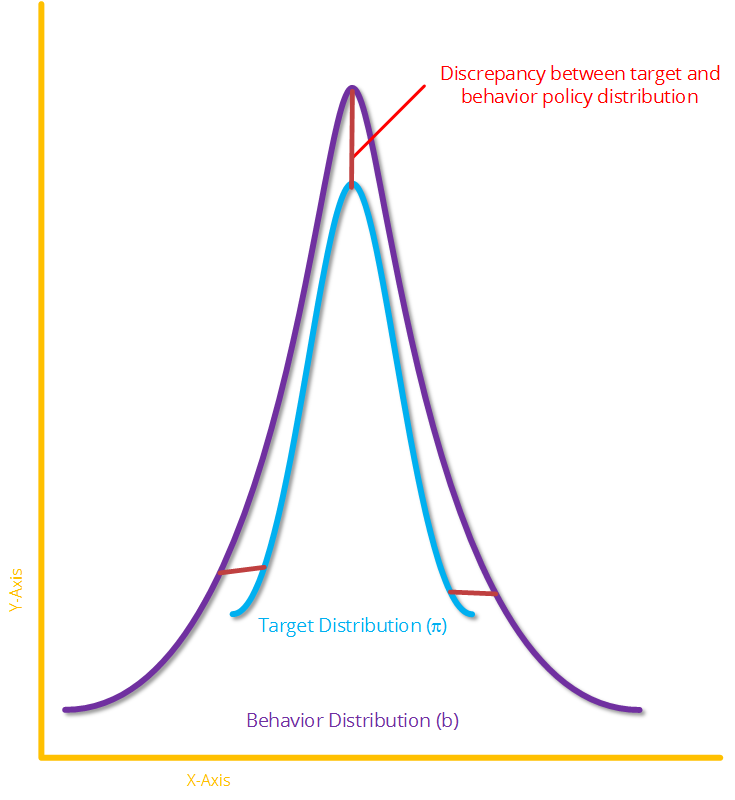
(a) The off-policy learning.

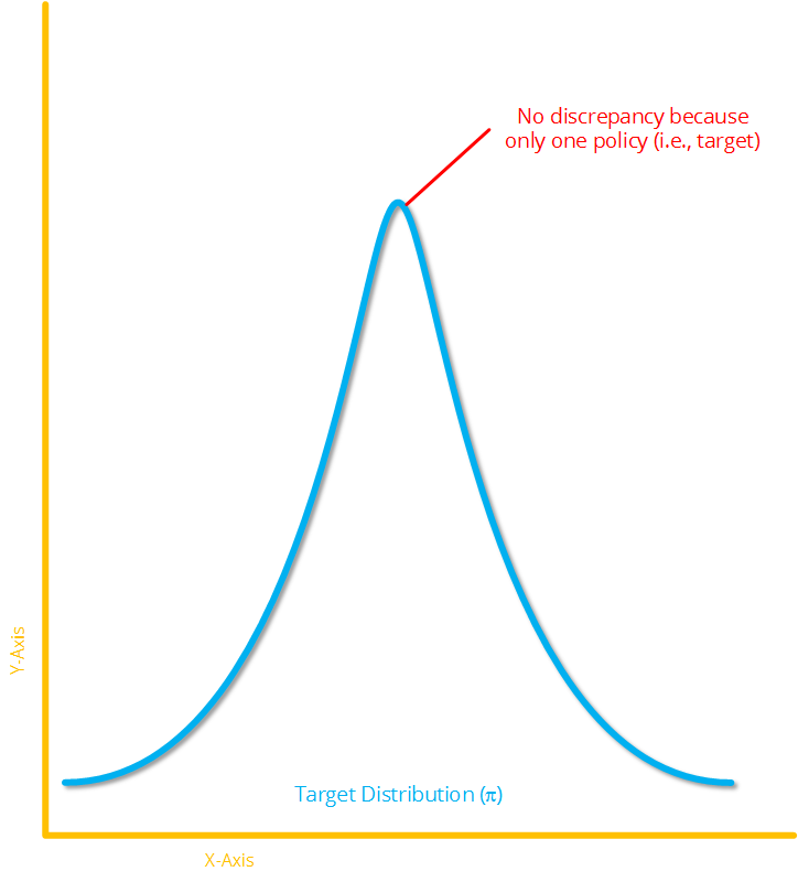
(b) The on-policy learning.

Figure 1: A comparison of on- and off-policy learning.

Rest of the paper is arranged as follows. Related works are discussed in section 2. In section 3, we present preliminaries. Section 4 & 5 show relative importance sampling and actor-critic model respectively. Section 6 presents experiments. Finally, we present a conclusion in section 7.

2 Related Work

2.1 On-Policy

Thomas (2014) claimed that biased discounted reward made natural actor-critic algorithms unbiased average reward natural actor-critics. Bhatnagar et al. (2009) presented four new online actor-critic reinforcement learning algorithms based on natural-gradient, function-approximation, and temporal difference learning. They also demonstrated the convergence of these four algorithms to a local maximum. Schaul et al. (2015) showed a framework for prioritizing experience, so as to replay significant transitions more often, and thus learned more efficiently. Bounded actions introduced bias when the standard Gaussian distribution was used as a stochastic policy. Chou et al. (2017) suggested using Beta distribution instead of Gaussian and examined the trade-off between bias and variance of policy gradient for both on- and off-policy.

Mnih et al. (2016) proposed four asynchronous deep RL algorithms. The most effective one was asynchronous advantage actor-critic (A3C), maintained a policy $\pi(a_{t}|s_{t};\theta)$ and an estimated of the value function $V(s_{t};\theta_{v})$. Van Seijen and Sutton (2014) introduced a true online TD($\lambda$) learning algorithm that was exactly equivalent to an online forward view and that empirically performed better than its standard counterpart in both prediction and control problem. Schulman et al. (2015a) developed an algorithm, called Trust Region Policy Optimization (TRPO) offered monotonic policy improvements and derived a practical algorithm with a better sample efficiency and performance. It was similar to natural policy gradient methods. Schulman et al. (2015b) developed a variance reduction method for policy gradient, called generalized advantage estimation (GAE) where a trust region optimization method used for the value function. The policy gradient of GAE significantly minimized variance while maintaining an acceptable level of bias. We are interested in off-policy learning rather than on-policy learning.

2.2 Off-Policy

Hachiya et al. (2009) considered the variance of value function estimator for off-policy methods to control the trade-off between bias and variance. Mahmood et al. (2014) used weighted importance sampling with function approximation and extended to a new weighted-importance sampling form of off-policy LSTD($\lambda$), called WIS-LSTD($\lambda$). Degris et al. (2012) proposed a method, named off-policy actor-critic (off-PAC) in which an agent learned a target policy while following and getting samples from a behavior policy. Gruslys et al. (2017) presented a sample-efficient actor-critic reinforcement learning agent, entitled Reactor. It used off-policy multi-step Retrace algorithm to train critic while a new policy gradient algorithm, called B-leave-one-out was used to train actor. Zimmer et al. (2018) showed a new off-policy actor-critic RL algorithm to cope with continuous state and actions spaces using the neural network. Their algorithm also allowed the trade-off between data-efficiency and scalability. Levine and Koltun (2013) talked to avoid ”poor local optima” in complex policies with hundreds of variable using ”guided policy search” (GPS). GPS used ”differential dynamic” programming to produce appropriate guiding samples, and defined a ”regularized importance sampled policy optimization” that integrated these samples into policy exploration.

Lillicrap et al. (2015) introduced a model-free, off-policy actor-critic algorithm using deep function approximators based on the deterministic policy gradient (DPG) that could learn policies in high-dimensional, continuous action spaces, called it deep deterministic policy gradient (DDPG). Wang et al. (2016) presented a stable, sample efficient actor-critic deep RL agent with ”experience replay”, called ACER that applied to both continuous and discrete action spaces successfully. ACER utilized ”truncate importance sampling with bias correction, stochastic dueling network architectures, and efficient trust region policy optimization” to achieve it. Munos et al. (2016) showed a novel algorithm, called Retrace($\lambda$) which had three properties: small variance, safe because of using samples collected from any behavior policy and efficient because it efficiently estimated Q-Function from off-policy. Gu et al. (2016) developed a method called Q-Prop that was both sample efficient and stable. It merged the advantages of on-policy (stability of policy gradient) and off-policy methods (efficiency). Model-free deep RL algorithms typical underwent from two major challenges: very high sample inefficient and unstable. Haarnoja et al. (2018) presented a soft actor-critic (SAC) method, based on maximum entropy and off-policy. Off-policy provided sample efficiency while entropy maximization provided stability. Most of these methods are similar to our method, but they use standard IS or entropy method whereas we use RIS. For a review of IS-off-Policy method, see the works of (Precup, 2000; Sutton et al., 2016; Jie and Abbeel, 2010; Elvira et al., 2015; Gu et al., 2017; van Hasselt et al., 2014; Precup et al., 2001).

3 Preliminaries

Markov decision process (MDP) is a mathematical formulation of RL problems. MDP is defined by tuples of objects, consisting of ($\mathcal{S}$, $\mathcal{A}$, $\mathcal{R}$, $\mathbb{P}$, $\gamma$). Where $\mathcal{S}$ is set of possible states, $\mathcal{A}$ is set of possible actions, $\mathcal{R}$ is distribution of reward given (state, action) pair, $\mathbb{P}$ is transition probability i.e. distribution of next state given (state, action) pair and $\gamma\in(0,1]$ is a discount factor. $\pi$ and b denote the target policy and behavior policy respectively. The policy ($\pi$) is a function from $\mathcal{S}$ to $\mathcal{A}$ that specifies what action to take in each state. An agent interacts with an environment over a number of discrete time steps in classical RL. At each time step t, the agent picks an action $a_{t}\in\mathcal{A}$ according to its policy ($\pi$) given its present state $s_{t}\in\mathcal{S}$. In return, the agent gets the next state $s_{t+1}\in\mathcal{S}$ according to the transition probability $\mathbb{P}(s_{t+1}|s_{t},a_{t})$ and observes a scalar reward $r_{t}(s_{t},a_{t})\in\mathcal{R}$. The process carries on until the agent arrives at the terminal state after which the process starts again. The agent outputs $\gamma$-discounted total accumulated return from each state $s_{t}$ i.e. $R_{t}=\begin{subarray}{c}\infty\\ \sum\\ k\geq 0\end{subarray}\gamma^{k}r(s_{t+k},a_{t+k})$.

In RL, there are two typical functions to select action following policy ($\pi$ or b): state-action value ($Q^{\pi}(s_{t},a_{t})=\mathbb{E}_{s_{t+1:\infty},a_{t+1:\infty}}[R_{t}|s_{t},a_{t}]$) and state value ($V^{\pi}(s_{t})=\mathbb{E}_{a_{t}\in\mathcal{A}}[Q^{\pi}(s_{t},a_{t})]$). $\mathbb{E}$ is expectation mean. Finally, the goal of the agent is to maximize the expected return ($J(\theta)=\mathbb{E}_{\pi}[R_{\theta}]$) using policy gradient ($\nabla_{\theta}J(\theta)$) with respect to parameter $\theta$. $J(\theta)$ is also called an objective or a loss function. The policy gradient of the objective function Sutton et al. (1999) which taking notation from Schulman et al. (2015b) is defined as:

$$\nabla_{\theta}J(\theta)=\mathbb{E}_{s_{0:\infty},a_{0:\infty}}\Bigg{[}\sum\limits_{\begin{subarray}{c}t\geq 0\end{subarray}}A^{\pi}(s_{t},a_{t})\ \nabla_{\theta}\ log\ \pi_{\theta}(a_{t}|s_{t})\Bigg{]}$$ (1)

Where $A^{\pi}(s_{t},a_{t})$ is an advantage function. Schulman et al. (2015b) has showed that we can use several expression in the place of $A^{\pi}(s_{t},a_{t})$ without introducing bias such as state-action value ($Q^{\pi}(s_{t},a_{t})$), the discounted return $R_{t}$ or the temporal difference (TD) residual ($r_{t}+\gamma V^{\pi}(s_{t+1})-V^{\pi}(s_{t})$). We use TD residual in our method. A classic policy gradient approximator with Rt has high variance and low bias whereas the approximator using function approximation has high bias and low variance (Wang et al., 2016). IS often has low bias but high variance (Sutton et al., 2016; Hachiya et al., 2009; Mahmood et al., 2014). We use RIS instead of IS. Merging advantage function with function approximation and RIS to achieve stable off-policy in RL. Policy gradient with function approximation denotes an actor-critic (Sutton et al., 1999) which optimizes the policy against the critic, e.g., deterministic policy gradient (Silver et al., 2014; Lillicrap et al., 2015).

4 Standard Importance Sampling

One reason for instability of off-policy learning is a discrepancy between distributions. In off-policy RL, we would like to gather data samples from the distribution of target policy but data samples are actually drawn from the distribution of the behavior policy. Importance sampling is a well-known approach to handle this kind of mismatch (Rubinstein and Kroese, 2016; Precup, 2000). For example, we would like to estimate the expected value of an action (a) at state (s) with samples drawn from the target policy ($\pi$) distribution while in reality, samples are drawn from another distribution i.e., behavior policy (b). A classical form of importance sampling can be defined as:

$$\mu=\mathbb{E}_{\pi}\{R(s,a)\} =\sum\limits_{\begin{subarray}{c}a\sim\pi\end{subarray}}\pi(a|s)R(s,a)$$ (2)

$$=\sum\limits_{\begin{subarray}{c}a\sim\pi\end{subarray}}\frac{\pi(a|s)}{b(a|s)}b(a|s)R(s,a)$$

$$=\mathbb{E}_{a\sim b}\left\{\frac{\pi(a|s)}{b(a|s)}R(s,a)\right\}$$

The importance sampling estimate of $\mu$ = $\mathbb{E}_{\pi}\{R(s,a)\}$ is

$$\hat{\mu}_{b}\approx\frac{1}{n}\sum\limits_{\begin{subarray}{c}t=1,a\sim b\end{subarray}}^{n}\frac{\pi(a_{t}|s_{t})}{b(a_{t}|s_{t})}R(s_{t},a_{t})$$ (3)

Where R(s,a) is a discounted reward function, $(s_{t},a_{t})$ are samples drawn from b and IS estimator ($\hat{\mu}_{b}$) computes an average of sample values.

4.1 Relative Importance Sampling

Although some research Wang et al. (2016); Precup et al. (2001); Gu et al. (2016) has been carried out on solving instability, no studies have been found that uses a smooth variant of IS in RL. The smooth variant of IS, such as RIS (Sugiyama, 2016; Yamada et al., 2011) is used to ease the instability in semi-supervised learning. Our quasi RIS can be defined as:

$$\mu_{\beta}=\frac{e^{\pi(a|s)}}{\beta e^{\pi(a|s)}+(1-\beta)e^{b(a|s)}}$$ (4)

This is one of the main contribution of this study. We use RIS in place of classical IS in our method. Then RIS estimate of $\mu_{\beta}$ = $\mathbb{E}_{\pi}\{R(a|s)\}$ is

$$\hat{\mu}_{\beta}\approx\frac{1}{n}\sum\limits_{\begin{subarray}{c}t\geq 0,a\sim b\end{subarray}}^{n}\frac{e^{\pi(a_{t}|s_{t})}}{\beta e^{\pi(a_{t}|s_{t})}+(1-\beta)e^{b(a_{t}|s_{t})}}R(a_{t}|s_{t})$$ (5)

Proposition 1

Since the importance is always non-negative, the relative importance is no greater than $\frac{1}{\beta}$:

$$\mu_{\beta}=\frac{1}{\beta+(1-\beta)\frac{e^{b(a|s)}}{e^{\pi(a|s)}}}\leq\frac{1}{\beta}$$ (6)

The proof is provided in Appendix E.

5 RIS-off-PAC Algorithm

An actor-critic algorithm applies to both on- and off-policy learning. However, our main focus is on off-policy learning. We present our algorithm for the actor and critic in this section. We also show a natural actor-critic version of our algorithm.

5.1 The Critic: Policy Evaluation

Let V be an approximate value function and can be defined as $V^{\pi}(s_{t})=\mathbb{E}_{a_{t}\in\mathcal{A}}[Q^{\pi}(s_{t},a_{t})]$. The TD residual of V with discount factor $\gamma$ (Sutton and Barto, 2018) is given as $\delta^{V^{\pi}}_{t}=r(s_{t},a_{t}\sim b(.|s_{t}))+\gamma V^{\pi}(s_{t+1})-V^{\pi}(s_{t})$). $b(.|s)$ is behavior policy probabilities for current state s. Policy gradient uses a value function ($V^{\pi}(s_{t})$) to evaluate a target policy ($\pi$). $\delta^{V^{\pi}}_{t}$ is considered as an estimate of $A^{\pi}_{t}$ of the action $a_{t}$ . i.e., $\delta^{V^{\pi}}_{t}\approx A^{\pi}_{t}$.

$$\mathbb{E}_{s_{t+1}}[\delta^{V^{\pi}}_{t}] =\mathbb{E}_{s_{t+1}}[r(s_{t},a_{t}\sim b(.|s_{t}))$$

$$+\gamma V^{\pi}(s_{t+1})-V^{\pi}(s_{t})]$$ (7)

$$=\mathbb{E}_{s_{t+1}}[Q^{\pi}(s_{t},a_{t})-V^{\pi}(s_{t})]$$

$$=A^{\pi}(s_{t},a_{t})$$

As can be seen from the above, an agent uses the action generated by the behavior policy instead of the target policy in our reward method. The approximated value function is trained to minimize the squared TD residual error.

$$J_{V}(\mathcal{\phi}) =\mathbb{E}_{s_{t+1}}[\frac{1}{2}(\delta^{V^{\pi}_{\phi}}_{t})^{2}]$$ (8)

5.2 The Actor: Policy Improvement

A critic updates action-value function parameter $\phi$. An actor updates policy parameter $\theta$ in the direction, recommended by the critic. The actor selects which action to take, and the critic conveys the actor how good its action was and how it should adjust its action. We can express the policy gradient in the following form.

$$J(\theta) =\mathbb{E}_{\pi}\Bigg{[}R(s,a)\Bigg{]}$$

$$\nabla J(\theta) =\hat{J}(\theta)=\nabla_{\theta}\mathbb{E}_{\pi}\Bigg{[}R(s,a)\Bigg{]}$$

$$\hat{J}(\theta) =\nabla_{\theta}\sum\limits_{\begin{subarray}{c}a\sim\pi\end{subarray}}\pi_{\theta}(a|s)R(s,a)$$

$$\hat{J}(\theta) =\sum\limits_{\begin{subarray}{c}a\sim\pi\end{subarray}}\nabla_{\theta}\pi_{\theta}(a|s)R(s,a)$$

$$\hat{J}(\theta) =\sum\limits_{\begin{subarray}{c}a\sim\pi\end{subarray}}\pi_{\theta}(a|s)\nabla_{\theta}\log\pi_{\theta}(a|s)R(s,a)$$

$$\hat{J}(\theta) =\sum\limits_{\begin{subarray}{c}a\sim\pi\end{subarray}}\pi_{\theta}(a|s)\nabla_{\theta}\log\pi_{\theta}(a|s)R(s,a)$$

$$\hat{J}(\theta) =\sum\limits_{\begin{subarray}{c}a\sim\pi\end{subarray}}\frac{\pi_{\theta}(a|s)}{b(a|s)}b(a|s)\nabla_{\theta}\log\pi_{\theta}(a|s)R(s,a)$$

From Equation 2, Expectation changes to the behavior policy.

$$\hat{J}(\theta) =\mathbb{E}_{b}\Bigg{[}\frac{\pi_{\theta}(a|s)}{b(a|s)}\nabla_{\theta}\log\pi_{\theta}(a|s)R(s,a)\Bigg{]}$$

In practice, we use an approximate TD error ($\delta^{V^{\pi}_{\phi}}$) to compute the policy gradient. The discounted TD residual ($\delta^{V^{\pi}_{\phi}}$) can be used to establish off-policy gradient estimator in the following form.

$$\hat{J}(\theta)=\frac{1}{N}\sum\limits_{\begin{subarray}{c}i=1\end{subarray}}^{N}\sum\limits_{\begin{subarray}{c}t=0\end{subarray}}^{\infty}\frac{\pi_{\theta}(a_{t}^{i}|s_{t}^{i})}{b(a_{t}^{i}|s_{t}^{i})}\nabla_{\theta}\ log\ \pi_{\theta}(a_{t}^{i}|s_{t}^{i})\delta^{V^{\pi,i}_{\phi}}_{t}$$ (9)

Our aim is to reduce instability of off-policy. The imbalance between bias and variance (large bias and large variance or small bias and large variance) is often likely to make off-policy unstable. IS reduces bias but introduces high variance. The reason is that IS ratio fluctuates greatly from sample to sample and IS averages the reward $R(a_{t}|s_{t})\frac{\pi(a_{t}|s_{t})}{b(a_{t}|s_{t})}$ that is of high variance (Hanna et al., 2018; Mahmood et al., 2014; Silver et al., 2014; Precup, 2000). Thus, a smooth variant of IS is required to mitigate high variance (high variance is directly proportional to instability) such as RIS. RIS has bounded variance and low bias. It has been proven by proposition 1 that RIS is bounded i.e. $\mu_{\beta}\leq\frac{1}{\beta}$, therefore, the variance of RIS is also bounded. IS reduces bias and RIS is the smooth variant of IS, thus, RIS also reduces bias (Hachiya et al., 2009; Gu et al., 2017; Mahmood et al., 2014; Sugiyama, 2016). Therefore, to minimize bias while maintaining bounded variance, we use off-policy case, where ($J(\theta)$) can be estimated using action drawn from $b(a|s)$ in place of $\pi(a|s)$ and combine RIS ratio $\mu_{\beta}$ with $\hat{J}(\theta)$ which we call RIS-off-PAC.

$$\hat{J}_{\mu_{\beta}}(\theta) =\frac{1}{N}\sum\limits_{\begin{subarray}{c}i=1\end{subarray}}^{N}\sum\limits_{\begin{subarray}{c}t=0\end{subarray}}^{\infty}(\frac{e^{\pi(a^{i}_{t}|s^{i}_{t})}}{\beta e^{\pi(a^{i}_{t}|s^{i}_{t})}+(1-\beta)e^{b(a^{i}_{t}|s^{i}_{t})}})$$

$$\quad\quad\quad\quad\quad\quad\nabla_{\theta}\ log\ \pi_{\theta}(a_{t}^{i}|s_{t}^{i})\delta^{V^{\pi,i}_{\phi}}_{t}$$

$$=\frac{1}{N}\sum\limits_{\begin{subarray}{c}i=1\end{subarray}}^{N}\sum\limits_{\begin{subarray}{c}t=0\end{subarray}}^{\infty}\mu^{i}_{t,\beta}\nabla_{\theta}\ log\ \pi_{\theta}(a_{t}^{i}|s_{t}^{i})\delta^{V^{\pi,i}_{\phi}}_{t}$$ (10)

Two important truths about an Equation (5.2) must be pointed out. First, we use RIS ($\frac{e^{\pi(a^{i}_{t}|s^{i}_{t})}}{\beta e^{\pi(a^{i}_{t}|s^{i}_{t})}+(1-\beta)e^{b(a^{i}_{t}|s^{i}_{t})}}$) instead of IS ($\frac{\pi_{\theta}(a_{t}^{i}|s_{t}^{i})}{b(a_{t}^{i}|s_{t}^{i})}$). Second, We use $\mu_{t,\beta}$ instead of $\prod\limits_{\begin{subarray}{c}t=0\end{subarray}}^{\infty}\mu_{t,\beta}$, therefore, it doesn’t involve a product of several unbounded important weights, but instead only need to approximate relative importance weight $\mu_{\beta}$. Bounded RIS is expected to demonstrate low variance. We present two variants of the actor-critic algorithm here: (i) relative importance sampling off-policy actor-critic (RIS-off-PAC) (ii) relative importance sampling off-policy natural actor-critic (RIS-off-PNAC).

  Initialize: policy parameters $\theta$, critic parameters $\phi$, discount factor ($\gamma$), done=false, t=0, $\alpha_{\theta},\alpha_{\phi},\beta\in[0,1]$

  for $i=1$ to $N$ do

     repeat

        Choose an action $(a_{t}^{i})$, according to $\pi(.|s_{t}^{i}),b(.|s_{t}^{i})$

        Observe output next state ($\acute{s}^{i}$), reward (r), and done

        $\mu^{i}_{t,\beta}=\frac{e^{\pi_{\theta}(a^{i}_{t}|s^{i}_{t})}}{\beta e^{\pi_{\theta}(a^{i}_{t}|s^{i}_{t})}+(1-\beta)e^{b(a^{i}_{t}|s^{i}_{t})}}$

        Update the critic:

        $\delta^{V^{\pi,i}_{\phi}}_{t}=r(s_{t}^{i},a_{t}^{i}\sim b(.|s_{t}^{i}))+\gamma V^{\pi}_{\phi}(\acute{s}^{i})-V^{\pi}_{\phi}(s_{t}^{i})$

        $\nabla_{\phi}J(\phi)\approx\frac{1}{2}\nabla_{\phi}\|\delta^{V^{\pi,i}_{\phi}}_{t}\|^{2}$

        $\phi=\phi+\alpha_{\phi}\nabla_{\phi}J(\phi)$

        Update the actor:

        $\nabla_{\theta}J_{\mu_{\beta}}(\theta)\approx\mu^{i}_{t,\beta}\ \nabla_{\theta}\ log\ \pi_{\theta}(a_{t}^{i}|s_{t}^{i})\ \delta^{V^{\pi,i}_{\phi}}_{t}$

        $\theta=\theta+\alpha_{\theta}\nabla_{\theta}J_{\mu_{\beta}}(\theta)$

        $t\ +=1$

        $s^{i}=\acute{s}^{i}$

     until $done$ is $false$

  end for

Algorithm 1 The RIS-off-PAC algorithm

Where in algorithm 1 & 2, $\alpha_{\theta}$ and $\alpha_{\phi}$ are learning rate for actor and critic respectively. State s represents current state while state $\acute{s}$ represents next state. The algorithm 2 is RIS-off-PNAC that is based on the natural gradient estimate $\hat{J}_{t}(\theta)=G_{t}^{-1}(\theta)\ \nabla_{\theta}\ log\ \pi_{\theta}(a_{t}|s_{t})\ \delta^{V^{\pi}_{\phi}}_{t}$. $G^{-1}_{t}(\theta)$ is the natural gradient and we refer to see (Bhatnagar et al., 2009; Konda and Tsitsiklis, 2003; Peters et al., 2005; Silver et al., 2014) for further details. The only difference between RIS-off-PAC and RIS-off-PNAC is that we use the natural gradient estimate in place of the regular gradient estimate in RIS-off-PNAC. RIS-off-PNAC algorithm 2 utilizes Equation 26 of Bhatnagar et al. (2009) to estimate the natural gradient. However, natural actor-critic (NAC) algorithms of Bhatnagar et al. (2009) are on-policy whereas our algorithm is off-policy. In RL, we want to maximize the rewards, thus, the optimization problem we consider here is a maximization instead of a minimization. So, we actual minimize a negative loss function, the negative of minimum loss function return maximum reward in the original problem.

  Initialize: policy parameters $\theta$, critic parameters $\phi$, discount factor ($\gamma$), done=false, t=0, $\alpha_{\theta},\alpha_{\phi},\beta\in[0,1],G_{0}=\mathbb{I}$

  for $i=1$ to $N$ do

     repeat

        Choose an action $(a_{t}^{i})$, according to $\pi(.|s_{t}^{i}),b(.|s_{t}^{i})$

        Observe output next state ($\acute{s}^{i}$), reward (r), and done

        $\mu^{i}_{t,\beta}=\frac{e^{\pi_{\theta}(a^{i}_{t}|s^{i}_{t})}}{\beta e^{\pi_{\theta}(a^{i}_{t}|s^{i}_{t})}+(1-\beta)e^{b(a^{i}_{t}|s^{i}_{t})}}$

        Update the critic:

        $\delta^{V^{\pi,i}_{\phi}}_{t}=r(s_{t}^{i},a_{t}^{i}\sim b(.|s_{t}^{i}))+\gamma V^{\pi}_{\phi}(\acute{s}^{i})-V^{\pi}_{\phi}(s_{t}^{i})$

        $\nabla_{\phi}J(\phi)\approx\frac{1}{2}\nabla_{\phi}\|\delta^{V^{\pi,i}_{\phi}}_{t}\|^{2}$

        $\phi=\phi+\alpha_{\phi}\nabla_{\phi}J(\phi)$

        Update the actor:

        $G^{-1}_{t}(\theta)=\frac{1}{1-\alpha_{\theta,t}}\Bigg{[}G^{-1}_{t-1}(\theta)-\alpha_{\theta,t}\frac{(G^{-1}_{t-1}(\theta)\nabla_{\theta}\log\pi_{\theta}(a_{t}^{i}|s_{t}^{i}))\ (G^{-1}_{t-1}(\theta)\nabla_{\theta}\log\pi_{\theta}(a_{t}^{i}|s_{t}^{i}))^{T}}{1-\alpha_{\theta,t}+\alpha_{\theta,t}(\nabla_{\theta}\log\pi_{\theta}(a_{t}^{i}|s_{t}^{i}))^{T}G^{-1}_{t-1}(\theta)\nabla_{\theta}\log\pi_{\theta}(a_{t}^{i}|s_{t}^{i})}\Bigg{]}$

        $\nabla_{\theta}J_{\mu_{\beta}}(\theta)\approx\mu^{i}_{t,\beta}\ \nabla_{\theta}\ log\ \pi_{\theta}(a_{t}^{i}|s_{t}^{i})\ G^{-1}_{t}(\theta)\ \delta^{V^{\pi,i}_{\phi}}_{t}$

        $\theta=\theta+\alpha_{\theta}\nabla_{\theta}J_{\mu_{\beta}}(\theta)$

        $t\ +=1$

        $s^{i}=\acute{s}^{i}$

     until $done$ is $false$

  end for

Algorithm 2 The RIS-off-PNAC algorithm

Lemma 1

The RIS estimator ($\hat{\mu}_{\beta}$) becomes the ordinary IS estimator ($\hat{\mu}_{b}$) if $\beta=0$.
The proof is provided in Appendix E.

Proposition 2

If $\beta=0$, the RIS off-policy gradient estimator becomes the ordinary IS off-policy gradient estimator.
The proof is provided in Appendix E.

Lemma 2

The RIS estimator produces uniform weight $\hat{\mu}_{\beta}=\frac{1}{1-\gamma}$ if $\beta=1$.
The proof is provided in Appendix E.

Lemma 3

The RIS produces uniform weight 1 if $\beta=1$.
The proof is provided in Appendix E.

Proposition 3

If $\beta=1$, the RIS off-policy gradient estimator becomes the ordinary on-policy gradient estimator.
The proof is provided in Appendix E.

Theorem 5.1

If $\beta=0$, then the variance of RIS estimator ($Var_{b}(\hat{\mu}_{\beta})$) is $\mathbb{E}_{b}[\hat{\mu}_{b}^{2}]$.
The proof is provided in Appendix E.

Remark 1

If $\beta=0$, lemma 1 shows that RIS estimator is equal to standard IS estimator. Theorem 5.1 also shows that variance of RIS estimator is also equal to standard IS estimator when $\beta=0$. Therefore, we conclude that if the expectation of RIS and standard IS are equal, then their variances are also equal.

Theorem 5.2

If $\beta=1$, Then, the variance of RIS estimator ($\hat{\mu}_{\beta})$) is $\frac{-2\gamma}{(1-\gamma^{2})(1-\gamma)}$.
The proof is provided in Appendix E.

Theorem 5.3

If $\beta=1$, Then, the variance of RIS is zero.
The proof is provided in Appendix E.

Remark 2

$\beta[0,1]$ controls the smoothness. The RIS ($\mu_{\beta}$) becomes the ordinary IS ($\frac{\pi(a|s)}{b(a|s)}$) if $\beta=0$. RIS becomes smoother if $\beta$ is increased, and it produces uniform weight $\mu_{\beta}=1$ if $\beta=1$. It is proved by lemma 1 and 3. Smoothness is directly proportional to the value of $\beta$. Variance decreases when smoothness rises. Therefore, Smoothness is directly proportional to the stability of off-policy. Thus, $\beta$ controls the stability of off-policy, as $\beta$ increases off-policy becomes more stable.

Remark 3

The RIS estimator $\hat{\mu}_{\beta}$ is a consistent unbiased estimator of $\pi$. $\hat{\mu}_{\beta}$ has bounded variance because RIS is bounded according to proposition 1. The standard IS estimator is unbiased, but it suffers from very high variance as it involves a product of many potentially unbounded importance weights (Wang et al., 2016; Hachiya et al., 2009). However, RIS has low variance as it does not involves a product of many unbounded weights.

5.3 RIS-Off-Policy Actor-critic Architecture

Figure 2(a) shows the RIS-off-PAC architecture. The difference between RIS-off-PAC and traditional actor-critic architecture (Sutton et al., 1999; Sutton and Barto, 2018) is that we introduce behavior policy based on RIS in our method, use action generated by $b(A|S)$ in reward function instead of $\pi(A|S)$. We compute RIS using both $\pi(A|S)$ and $b(A|S)$ policy into an actor, therefore, we pass samples from $b(A|S)$ to the actor as shown in Figure 2(a). TD error and others are same as a traditional actor-critic method.

Figure 2(b) shows the RIS-off-PAC neural network (NN) architecture. We use control RL tasks: CartPole-v0, LunarLander-v2, MountainCar-v0, and Pendulum-v0 for our experiment. We apply our RIS-off-PAC-NN on all of these tasks. Details of our NN as follows: In our architecture, we have a target network (Actor), value network (Critic) and off-policy network (behavior policy). Each of them implemented as a fully connected layer using TensorFlow as shown in Figure 2(b). Each NN contains inputs layer, 2 hidden layers: hidden layer 1 and hidden layer 2, and an output layer. Hidden layer 1 has 24 neurons (units) for all three Network for all RL task. Hidden layer 2 has a single neuron in the value network for all RL task. A number of neurons in hidden layer 2 for target network and off-policy network are equal to a number of actions available in given RL task. Hidden layer 1 employs RELU activation function in target and value network while CRELU activation function used in the off-policy network. Hidden layer 2 utilizes SOFTMAX activation function in target and off-policy network whereas it uses no activation function in the value network. Weight W is generated using the ”he_uniform” function of TensorFlow for all NN and tasks. We availed AdamOptimizer for learning neural network parameters for all RL tasks. $\beta$ is generated uniform random values between 0 and 1. We set numpy random seed, TensorFlow random seed and OpenAI Gym environment seed to 1 to reproduce results.

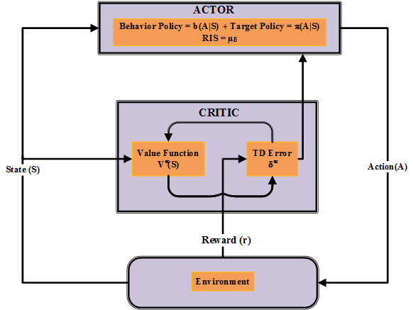
(a) The RIS-Off-PAC Architecture.

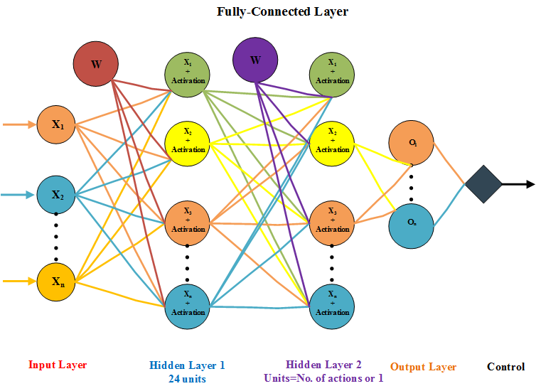
(b) The RIS-Off-PAC Neural Network Architecture.

Figure 2: Illustration of RIS-Off-PAC Architectures.

6 Experimental Setup

We conducted experiments on OpenAI Gym control tasks. The environments were shown in Figure 3. Our experiments run on a single machine with 16 GB memory, Intel Core i7-2600 CPU, and no GPU. We used operating system: 64-bit Ubuntu 18.04.1 LTS, programming language: python 3.6.4, library: TensorFlow 1.7, and OpenAI Gym library (Brockman et al., 2016).

(a) CartPole v0

(b) LunarLander v2

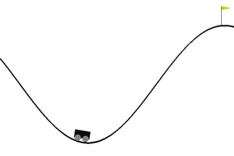
(c) MountainCar v0

(d) Pendulum v0

Figure 3: OpenAI Gym control used for all experiments. In order from the left to right: CartPole, LunarLander, MountainCar, and Pendulum. Detailed descriptions of each environment are provided in the appendix A, B, C, and D.

6.1 Experimental Results

We evaluated RIS-off-PAC/RIS-off-PNAC algorithm on four OpenAI Gym’s environments: CartPole-v0, LunarLander-v2, MountainCar-v0, and Pendulum-v0. We compared the proposed methods with the following algorithms: asynchronous advantage actor-critic (A3C) Mnih et al. (2016), proximal policy optimization (PPO) Schulman et al. (2017), and policy gradient soft-max (PG) (Sutton and Barto, 2018, Chapter 13).

The goal of CartPole-v0 is to prevent the pole from falling over as long as possible. We use a maximum of 300 episodes for each algorithm. Learning curves in Figure 4(a) for CartPole problem showing the averaged reward of each algorithm. From the Figure 4(a) we can see that RIS-off-PNAC algorithm outperforms all algorithms. The RIS-off-PAC, A3C, PPO, and PG secure second, third, fourth, and fifth positions respectively in terms of performance. The results of RIS-off-PAC and RIS-off-PNAC algorithm using different values of $\beta$ are shown in Figure 5(a) & 5(b) respectively. Overall, both algorithms show a similar kind of performance and stability for all values of $\beta$ except for $\beta=0.1,0.4$ in RIS-off-PAC and $\beta=0.3$ in RIS-off-PNAC.

The aim of LunarLander-v2’s agent is to land the lander safely on the landing pad. Each algorithm harnesses maximum of 300 episodes. Figure 4(b) presents the averaged reward of each algorithm. As shown in Figure 4(b), RIS-off-PAC outperforms all algorithms except for the RIS-off-PNAC and A3C algorithm but its performance is comparable to theirs. The performance of RIS-off-PNAC algorithm is superior to all other algorithms. The results obtained from the RIS-off-PAC and RIS-off-PNAC algorithm using different values of $\beta$ are setout in Figure 6(a) & 6(b). On the whole, the results of RIS-off-PAC algorithm for all values of $\beta$ except for $\beta=0.8,0.9$ are stable and almost identical. Similarly, the results of RIS-off-PNAC algorithm for all values of $\beta$ are quite stable and very close to each other.

The objective of MountainCar-v0 is to drive up on the right and reach on the top of the mountain with minimum episodes and steps. We use a maximum of 100 episodes for each algorithm. Figure 7(a) shows the averaged reward of all algorithms. As shown in Figure 7(a), The RIS-off-PAC and RIS-off-PNAC outperform all algorithms. The results of RIS-off-PAC and RIS-off-PNAC are quite similar. The results of RIS-off-PAC and RIS-off-PNAC algorithm using different values of $\beta$ are shown in Figure 8(a) & 8(b) respectively. By and large, the outcomes of RIS-off-PNAC are the most stable for all values of $\beta$ as can be seen from Figure 8(b). From Figure 8(a) we can see that the results of RIS-off-PAC are also stable for all values of $\beta$.

The target of Pendulum-v0 is to keep a frictionless pendulum standing up for as long as possible. Maximum 1000 episodes have been used to achieve this goal. Learning curves of the averaged reward for each algorithm are presented in Figure 7(b). It can be seen from the Figure 7(b) that the performance of RIS-off-PNAC is superior to all algorithms while the performance of RIS-off-PAC is poor compared to the RIS-off-PNAC but better than the remaining algorithms. The Figure 9(a) & 9(b) show the results of RIS-off-PAC and RIS-off-PNAC algorithm using different values of $\beta$. In general, as it has been shown in Figure 9(b), the results of RIS-off-PNAC are the most stable for all values of $\beta$ while the Figure 9(a) demonstrates that the results of RIS-off-PAC are also stable for all values of $\beta$.

The average rewards for last 100-episodes of each algorithm with their respective environments are summarized in Table 1. It is evident that the best performer is RIS-off-PNAC in CartPole, LunarLander, and Pendulum tasks, which with 1386.66, -2.80, and -3.78 averaged rewards respectively. RIS-off-PAC outperforms all algorithm in MountainCar task. In LunarLander task, A3C algorithm is the second best performer, gaining -6.05 averaged reward compared to -10.43 averaged reward of RIS-off-PAC. The reason that RIS-off-PAC does not perform better than A3C in LunarLander task may be a learning rate value. The performance of RIS-off-PAC might improve in LunarLander task by adjusting the learning rate value.

$\beta$ controls the smoothness, which helps to ease instability. The instability mitigation depends on the choice of the smoothness of $\beta$. Off-policy becomes more stable when RIS is smoother. RIS gets smoother when $\beta$ increases. Taking everything into consideration, we observe from the Figures 5(a), 5(b), 6(a), 6(b), 8(a), 8(b), 9(a), and 9(b) that the averaged rewards of RIS-off-PAC and RIS-off-PNAC algorithm are high when the value of $\beta$ is high. Especially when the value of $\beta$ is greater than or equal to 3, RIS-off-PAC/RIS-off-PNAC performs better, with the exception of some $\beta$ values in some environments. This suggests that higher values of $\beta$ minimize instability and maximize reward. Our experiments confirm that our off-policy algorithms achieve better or comparable performance to other algorithms. Videos of the policies learned with CartPole-v0, LunarLander-v2, MountainCar-v0, and Pendulum-v0 for RIS-off-PAC/RIS-off-PNAC algorithm are available online. Browse below footnote link to watch videos.

(a) CartPole

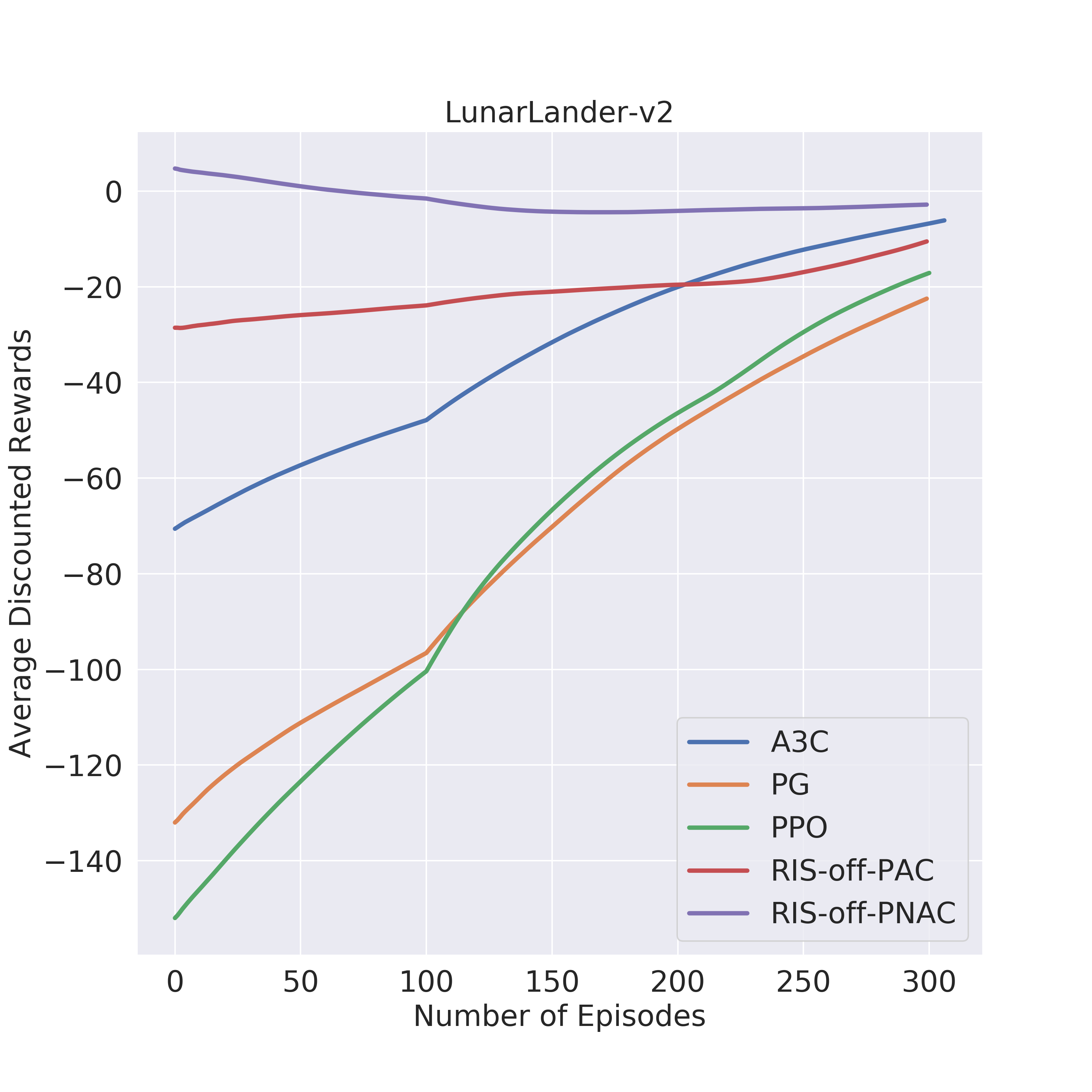
(b) LunarLander

Figure 4: (a) Training summary of all algorithms of CartPole. (b) Training summary of all algorithms of LunarLander. The x-axis shows the total number of training episodes. The y-axis shows the averaged rewards over 300 episodes.

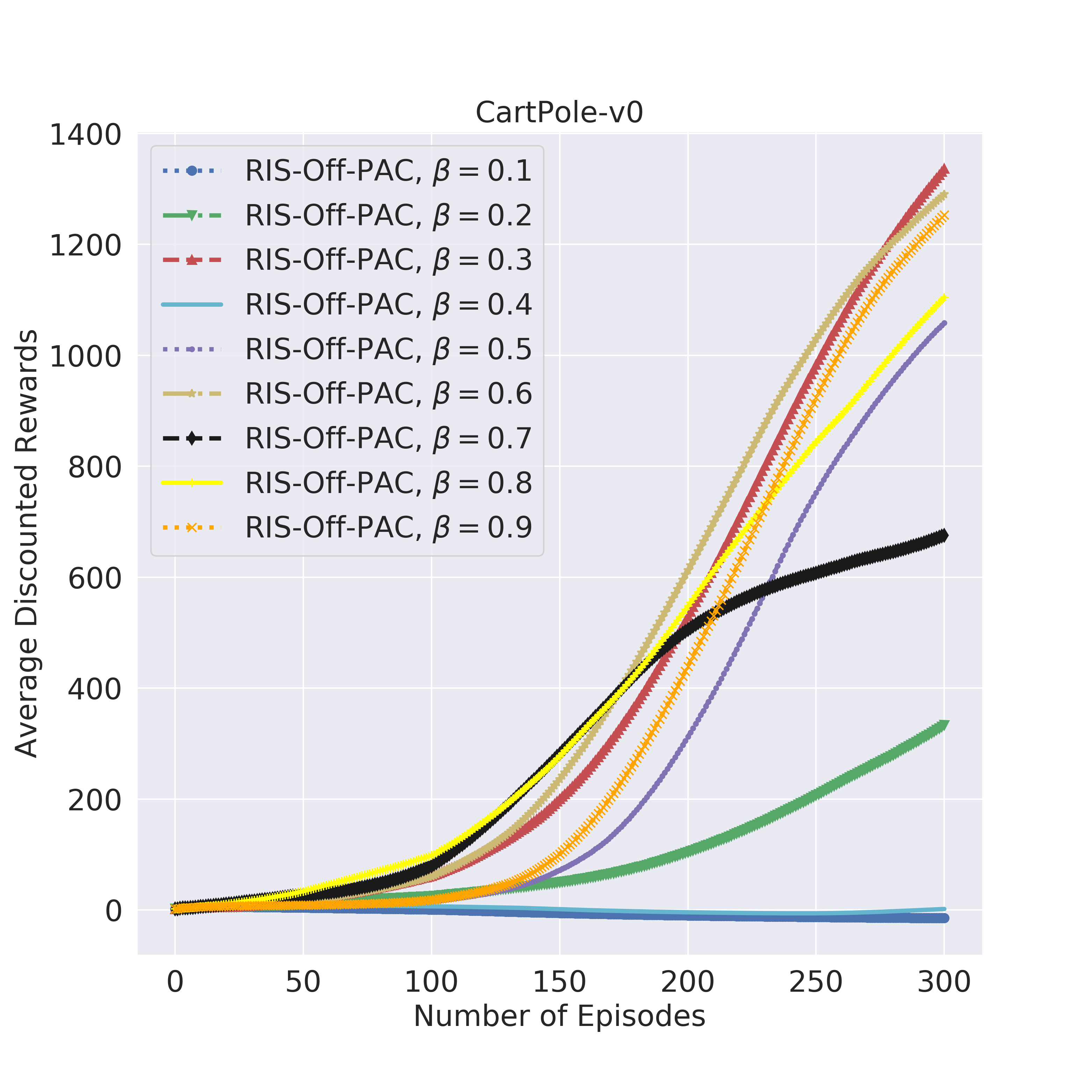
(a) RIS-0ff-PAC Algorithm

(b) RIS-0ff-PNAC Algorithm

Figure 5: (a), (b) Training summary of RIS-off-PAC and RIS-off-PNAC respectively for different value of $\beta\in[0,1]$. The x-axis shows the total number of training episodes. The y-axis shows the averaged rewards over 300 episodes.

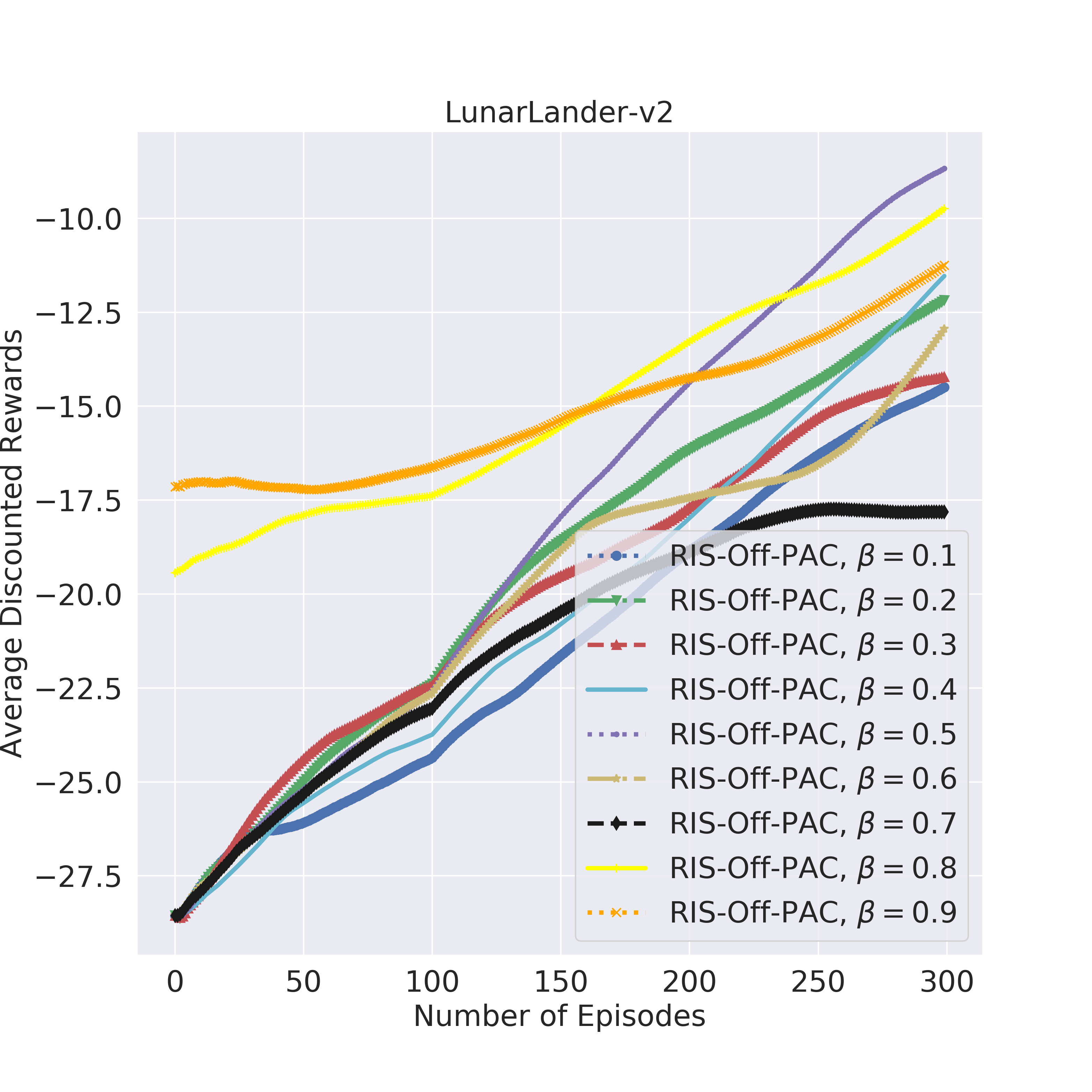
(a) RIS-off-PAC Algorithm

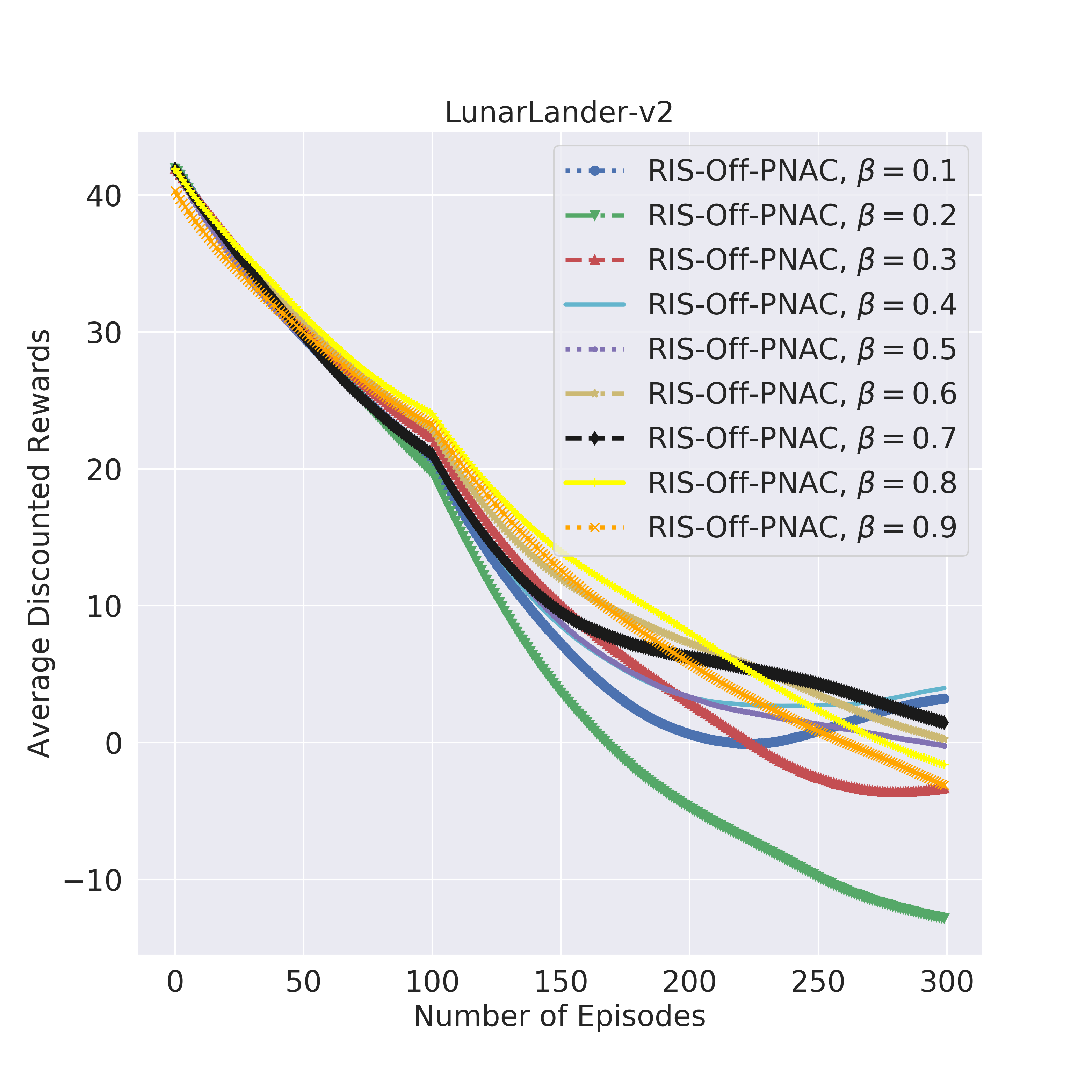
(b) RIS-off-PNAC Algorithm

Figure 6: (a), (b) Training summary of RIS-off-PAC and RIS-off-PNAC respectively for different value of $\beta\in[0,1]$. The x-axis shows the total number of training episodes. The y-axis shows the averaged rewards over 300 episodes.

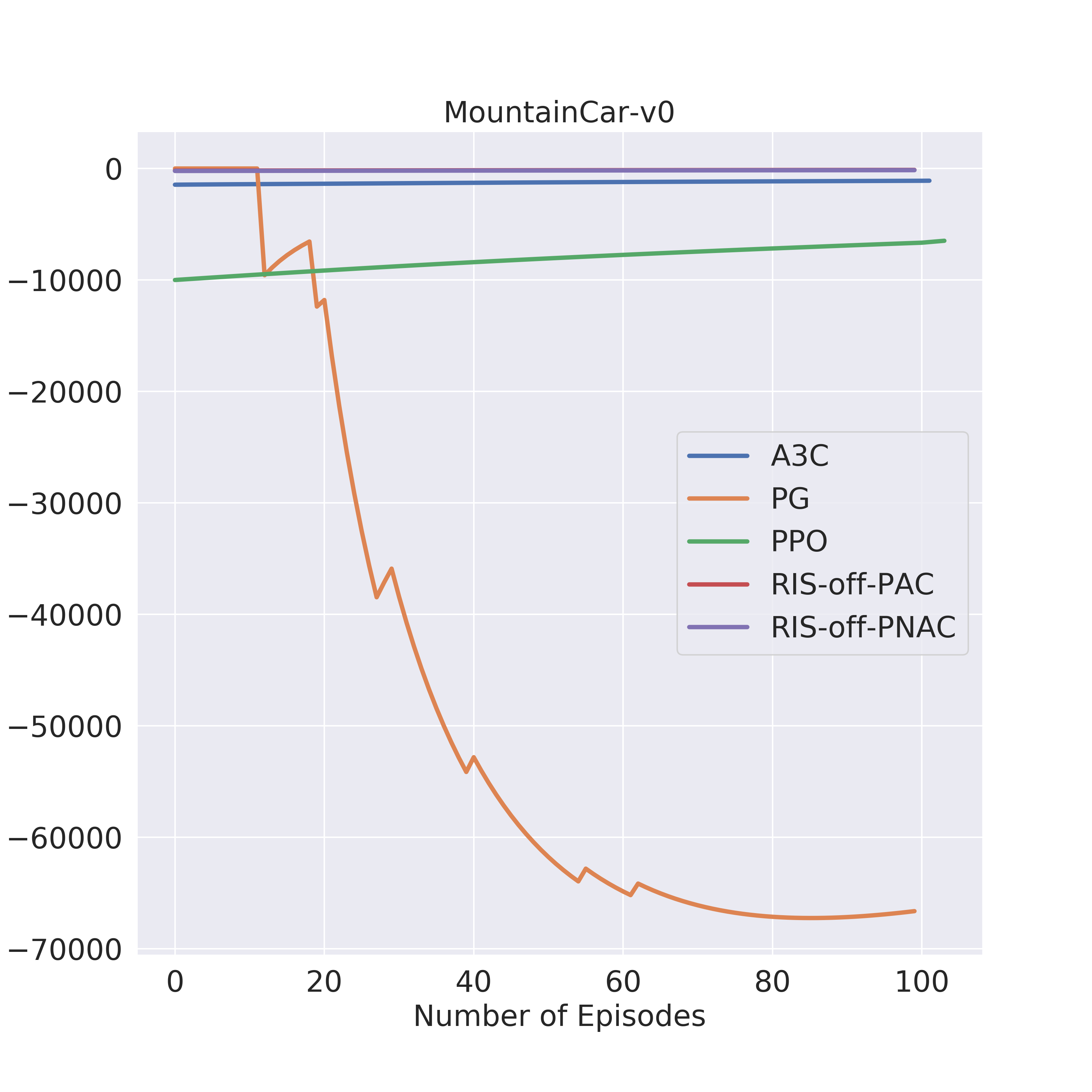
(a) MountainCar

(b) Pendulum

Figure 7: (a) Training summary of all algorithms of MountainCar. (b) Training summary of all algorithms of Pendulum. The x-axis shows the total number of training episodes. The y-axis denotes the averaged rewards for MountainCar and Pendulum over 100 and 1000 episodes respectively.

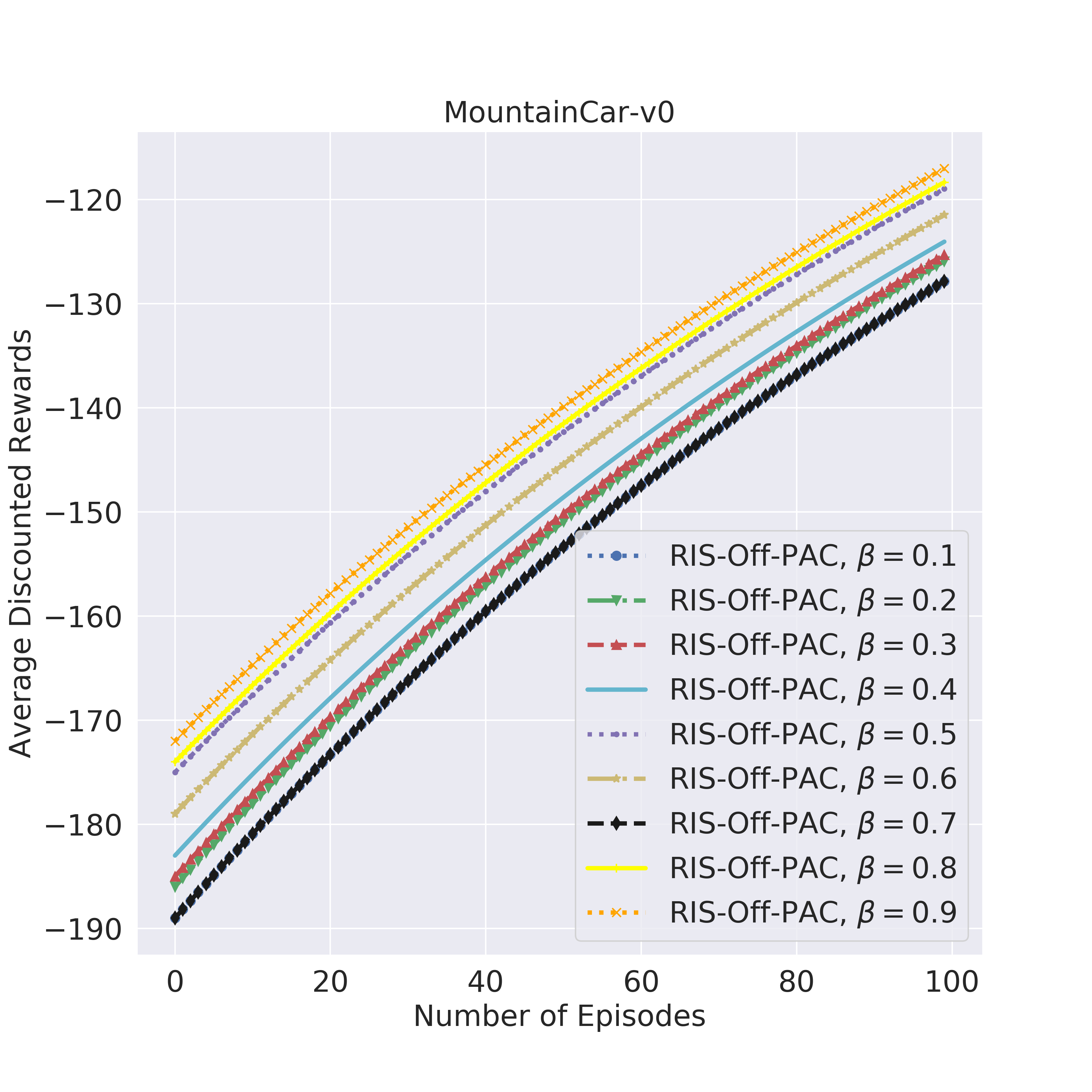
(a) RIS-off-PAC Algorithm

(b) RIS-off-PNAC Algorithm

Figure 8: (a), (b) Training summary of RIS-off-PAC and RIS-off-PNAC respectively for different value of $\beta\in[0,1]$. The x-axis shows the total number of training episodes. The y-axis shows the averaged rewards over 100 episodes.

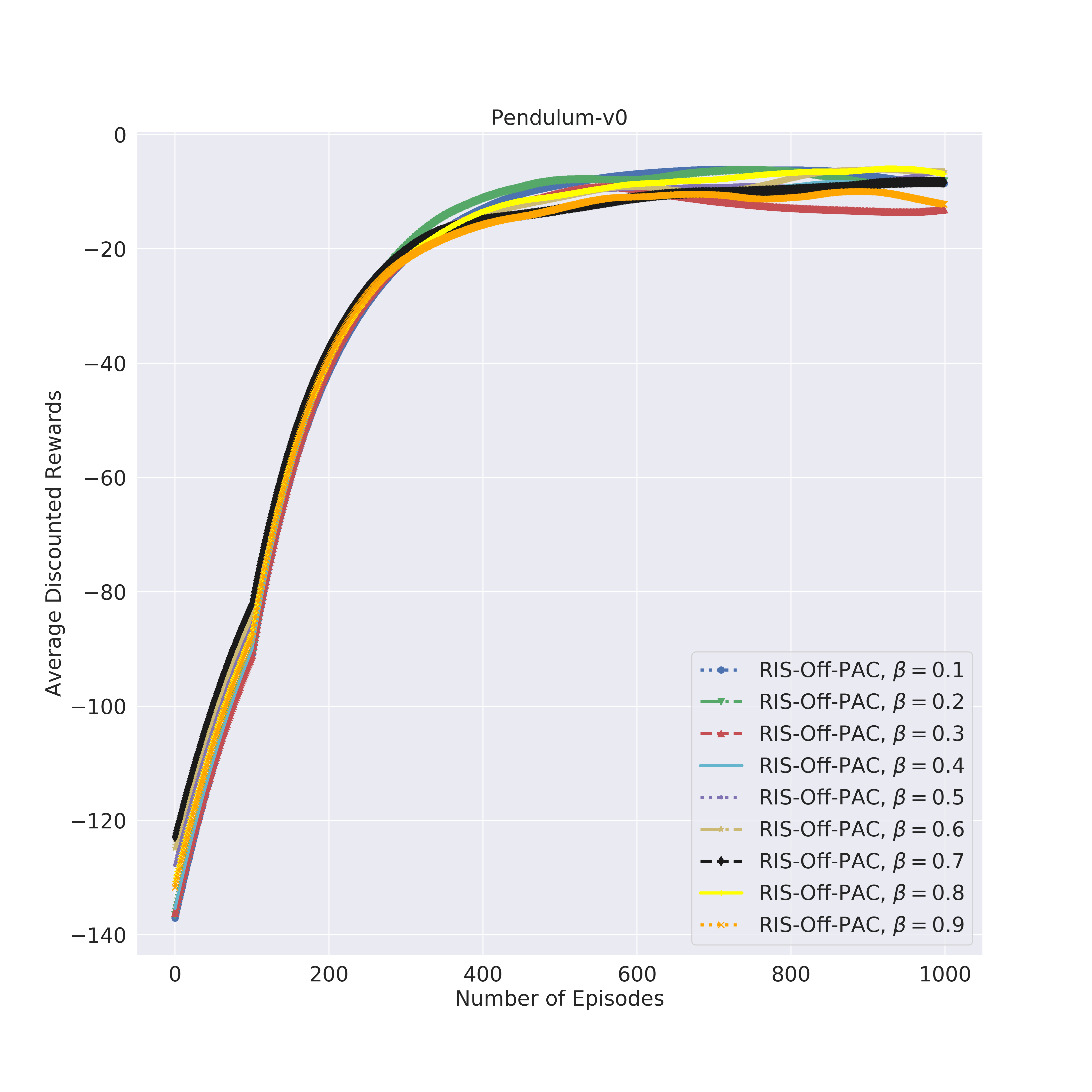
(a) RIS-off-PAC Algorithm

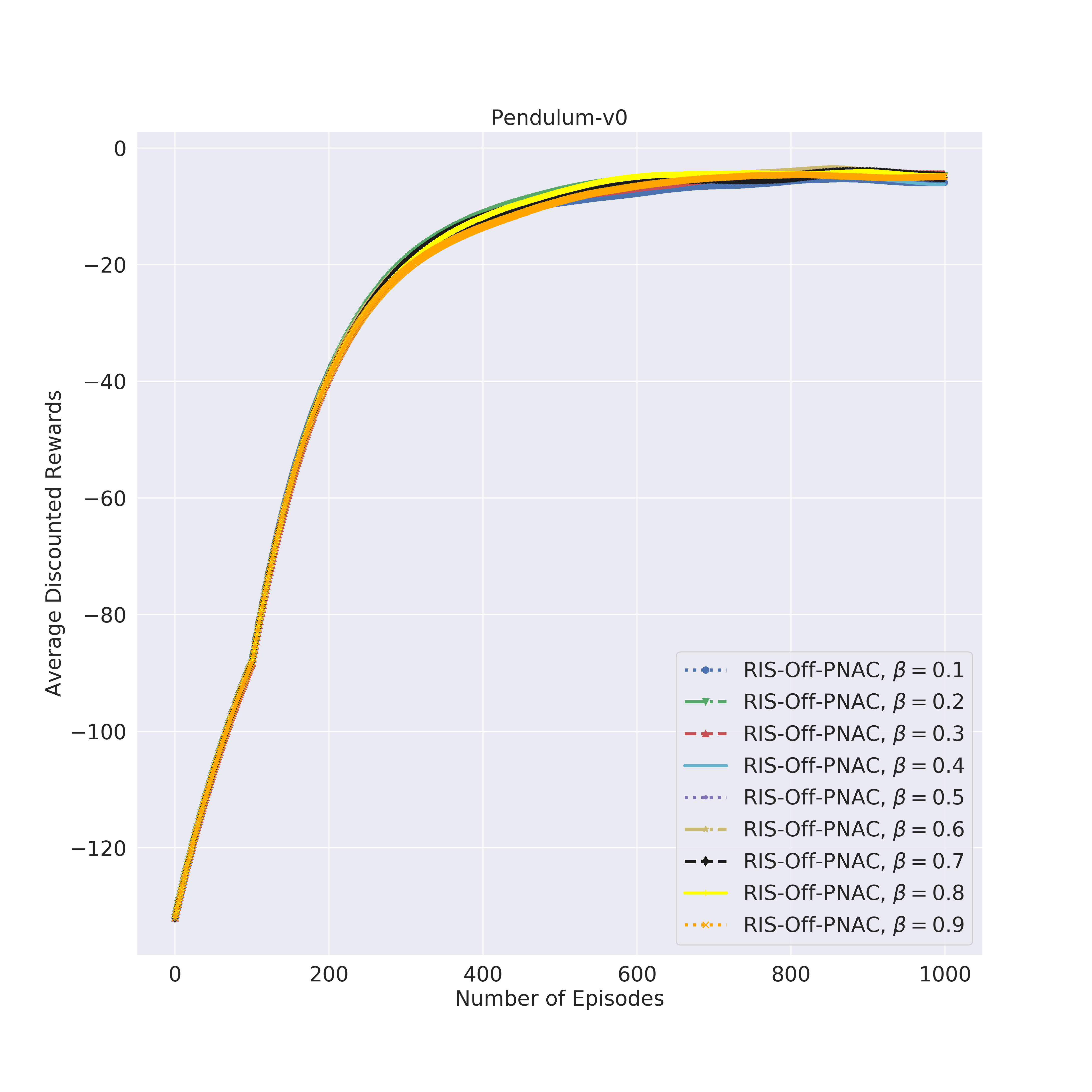
(b) RIS-off-PNAC Algorithm

Figure 9: (a), (b) Training summary of RIS-off-PAC and RIS-off-PNAC respectively for different value of $\beta\in[0,1]$. The x-axis shows the total number of training episodes. The y-axis shows the averaged rewards over 1000 episodes.

Table 1: Comparison of algorithm performance across CartPole-v0, LunarLander-v2, MountainCar-v0, Pendulum-v0.

	Environments
Last 100-Episodes Average Reward	CartPole-v0	LunarLander-v2	MountainCar-v0	Pendulum-v0
A3C	1147.20	-6.05	-1089.51	-11.43
PG	100.80	-22.34	-66613.21	-154.02
PPO	158.59	-16.98	-6448.20	-13.99
RIS-off-PAC	1176.27	-10.43	-124.66	-6.18
RIS-off-PNAC	1386.66	-2.80	-146.80	-3.78

7 Conclusions

We have shown off-policy actor-critic reinforcement learning algorithms based on RIS. It has achieved better or similar performance than state of the art methods. This method mitigates the instability of off-policy learning. In addition, our algorithm robustly solves classic RL problems such as CartPole-v0, LunarLander-v2, MountainCar-v0, and Pendulum-v0. A future work is to extend this idea to weighted RIS.

Appendices

Appendix A CartPole v0

CartPole is a famous benchmark for evaluating RL algorithms shown in Figure 3(a). The cart-pole environment used here is described by Barto et al. (1983). A cart moves along a frictionless track while balancing a pole. The pole starts upright, and the goal is to stop it from falling over by increasing and decreasing the cart’s velocity. A reward of +1 is given for every time step that the pole remains upright. We have two actions $a\in\{0=\textit{Push cart to the left},1=\textit{Push cart to the right}\}$ which are used the values of the force applied to the cart. The state S is defined as $s=[x,\dot{x},\theta,\dot{\theta}]\ where\ Cart\ Position=x\in[-2.4,2.4],\ Cart\ Velocity=\dot{x}\in[-\infty,\infty],\ Pole\ Angle=\theta\in[-41.8^{\circ},41.8^{\circ}],Pole\ Velocity\ At\ Tip=\dot{\theta}\in[-\infty,\infty]$. We obtained our result by using the following value of parameters:
A3C: we used learning rates of $10^{-3}$ and $10^{-3}$ for actor and critic respectively. $\gamma=0.9$.
PPO: we used learning rates of $10^{-4}$ and $10^{-4}$ for actor and critic respectively. $\gamma=0.9$.
PG: we used learning rates of $2\times 10^{-2}$. $\gamma=0.99$.
RIS-Off-PAC: we used learning rates of $2\times 10^{-2}$, $5\times 10^{-3}$ and $2\times 10^{-2}$ for actor, critic and off-policy network respectively. $\gamma=0.99$.
RIS-Off-PNAC: we used learning rates of $4\times 10^{-2}$, $10^{-3}$ and $4\times 10^{-2}$ for actor, critic and off-policy network respectively. $\gamma=0.99$.
We run for 1000 time steps and the episode ends when the pole is more than $\pm 12$ degrees from vertical, or the cart travels more than $\pm 2.4$ units from the center or if getting average reward of 195.0 over 100 consecutive episodes or if 1000 iteration completed. Our reward function is defined as

$$r(s_{t},a_{t},\acute{s})=\begin{cases}+160\textit{ If the cart reached its goal},\\ 1.0\textit{ Otherwise (for every time step).}\end{cases}$$

Where $a_{t}\in\mathcal{A}$ is the action chosen at the time t, $s_{t}\in\mathcal{S}$ is state at time t and $\acute{s}\in\mathcal{S}$ is next state at time t+1.

Appendix B LunarLander-v2

LunarLender is a well-known benchmark for examining RL tasks shown in Figure 3(b). In the LunarLender-v2 environment, an agent tries to land a craft smoothly on a landing pad. If the craft hits the ground with too much speed, the craft bursts. The agent is given a continuous vector that describes its state, and it also acts to turn on or off its engine. The landing pad is placed at the center of the screen, and if the craft lands on the landing pad, it is given reward. The agent chooses one of four actions: nothing, fire left orientation engine, fire main engine, and fire right orientation engine. The goal is to land the craft smoothly in the landing zone. Therefore, a reward between 100 and 140 is given when it lands near zero speed. When it lands on the target location and rests, it gets an extra + 100 points. When it crashes on the surface, it gets -100 points as a penalty. Firing main engine cost 0.3. Each leg of the craft contact on the ground gives +10 points. This problem is solved when obtaining a score of 200 points or higher on average over 100 consecutive landing attempts. We obtained our result by using the following value of parameters:
A3C: we used learning rates of $10^{-3}$ and $5\times 10^{-3}$ for actor and critic respectively. $\gamma=0.99$.
PPO: we used learning rates of $2\times 10^{-2}$ and $2\times 10^{-2}$ for actor and critic respectively. $\gamma=0.99$.
PG: we used learning rates of $2\times 10^{-2}$. $\gamma=0.99$.
RIS-Off-PAC: we used learning rates of $5\times 10^{-4}$, $10^{-3}$ and $5\times 10^{-3}$ for actor, critic and off-policy network respectively. $\gamma=0.99$.
RIS-Off-PNAC: we used learning rates of $2\times 10^{-4}$, $10^{-3}$ and $2\times 10^{-3}$ for actor, critic and off-policy network respectively. $\gamma=0.99$.
We run for 200 time steps and the episode terminates when the car reaches its target at top=0.5 position or if getting average reward of -110.0 over 100 consecutive episodes or if 200 iterations completed. Our reward function is defined as

$$r(s_{t},a_{t},\acute{s})=\begin{cases}-10\textit{ If the lander crashed},\\ default\ value\textit{ Otherwise (for every time step).}\end{cases}$$

Where $a_{t}\in\mathcal{A}$ is the action chosen at the time t, $s_{t}\in\mathcal{S}$ is state at time t and $\acute{s}\in\mathcal{S}$ is next state at time t+1.

Appendix C MountainCar v0

Mountain car is another famous benchmark for analyzing RL problems shown in Figure 3(c). Moore (1991) first presented this problem in his PhD thesis. A car is stationed between two hills. The goal is to drive up the hill on the right and reach to the top of the hill (top = 0.5 position). However, the car’s engine is inadequate power to climb up the hill in a single pass. Therefore, the only way to accomplish this task is to drive back and forth to boost momentum. We have three actions $a\in\{0=push\ left,1=no\ push,2=push\ right\}$ which are used the values of the force applied to the car. The state S is defined as $s=[x,\dot{x}]^{T}\ where\ position=x\in[-1.2,0.6],\ velocity=\dot{x}\in[-0.7,0.7]\}$. We obtained our result by using the following value of parameters:
A3C: we used learning rates of $10^{-3}$ and $5\times 10^{-3}$ for actor and critic respectively. $\gamma=0.9$.
PPO: we used learning rates of $10^{-4}$ and $10^{-4}$ for actor and critic respectively. $\gamma=0.9$.
PG: we used learning rates of $2\times 10^{-2}$. $\gamma=0.995$.
RIS-Off-PAC: we used learning rates of $5\times 10^{-3}$, $5\times 10^{-3}$ and $10^{-3}$ for actor, critic and off-policy network respectively. $\gamma=0.99$.
RIS-Off-PNAC: we used learning rates of $10^{-4}$, $10^{-3}$ and $10^{-4}$ for actor, critic and off-policy network respectively. $\gamma=0.99$.
We run for 200 time steps and the episode terminates when the car reaches its target at top=0.5 position or if getting average reward of -110.0 over 100 consecutive episodes or if 200 iterations completed. Our reward function is defined as

$$r(s_{t},a_{t},\acute{s})=\begin{cases}-20\textit{ If the car reached its goal i.e. $x_{\acute{s}}\geq 0.5$},\\ -1.0\textit{ Otherwise (for every time step).}\end{cases}$$

Where $a_{t}\in\mathcal{A}$ is the action chosen at the time t, $s_{t}\in\mathcal{S}$ is state at time t and $\acute{s}\in\mathcal{S}$ is next state at time t+1.

Appendix D Pendulum v0

The inverted pendulum swing is a well-known benchmark for assessing RL problems shown in Figure 3(d). In this version of the problem, the pendulum starts in a random position, and our goal is to swing it upwards so that it stands upright. Here are the details of the environment. The observation $s=(\cos{\theta},\sin{\theta},\dot{\theta})$ where $\theta\in[−\pi,\pi]$ is the angle of the pendulum and $\dot{\theta}\in[−8,8]$ is the angular velocity and the action $a\in[−2.0,2.0]$. The following equation is used to compute the reward. $r(s_{t},a_{t},\acute{s})=−(\theta^{2}+0.1*\dot{\theta}^{2}+0.001*a^{2})$. The lowest reward is $-(\pi^{2}+0.1*8^{2}+0.001*2^{2})=-16.2736044$ and the highest reward is 0. Episodes will terminate when task is done or it reaches above 200 steps. We obtained our result by using the following value of parameters:
A3C: we used learning rates of $10^{-4}$ and $10^{-3}$ for actor and critic respectively. $\gamma=0.9$.
PPO: we used learning rates of $10^{-4}$ and $2\times 10^{-4}$ for actor and critic respectively. $\gamma=0.9$.
PG: we used learning rates of $2\times 10^{-2}$. $\gamma=0.99$.
RIS-Off-PAC: we used learning rates of $5\times 10^{-3}$, $5\times 10^{-3}$ and $10^{-3}$ for actor, critic and off-policy network respectively. $\gamma=0.99$.
RIS-Off-PNAC: we used learning rates of $10^{-3}$, $10^{-3}$ and $10^{-4}$ for actor, critic and off-policy network respectively. $\gamma=0.99$.
We run for 200 time steps and the episode terminates when the car reaches its target at top=0.5 position or if getting average reward of -110.0 over 100 consecutive episodes or if 200 iterations completed. Our reward function is defined as

$$r(s_{t},a_{t},\acute{s})=\begin{cases}r\div 10\textit{ for every time step.}\end{cases}$$ (11)

Where $a_{t}\in\mathcal{A}$ is the action chosen at the time t, $s_{t}\in\mathcal{S}$ is state at time t and $\acute{s}\in\mathcal{S}$ is next state at time t+1.

Appendix E PROOFS

Proof

proposition 1

Let $$\beta\in[0,1] \pi(a|s)\ and\ b(a|s)>0 \pi(a|s)=b(a|s)\ or\ \pi(a|s)>b(a|s)\ or\ \pi(a|s)<b(a|s) \mu_{\beta}\leq\frac{1}{\beta} \pi(a|s)=b(a|s)$$ such that . For , for all such conditions, . We show the proof of below and the proof of remaining conditions can be done in similar way.

Let $$\pi(a|s)=\infty b(a|s)=\infty$$ and

$$\mu_{\beta} =\frac{1}{\beta+(1-\beta)\frac{e^{\infty}}{e^{\infty}}}\leq\frac{1}{\beta}$$

$$\mu_{\beta} =\frac{1}{\beta+(1-\beta)\frac{\infty}{\infty}}\leq\frac{1}{\beta}\text{\quad Where $e^{\infty}=\infty$.}$$

$$\mu_{\beta} =\frac{1}{\beta+(1-\beta)\infty}\leq\frac{1}{\beta}$$

$$\mu_{\beta} =\frac{1}{\infty}\leq\frac{1}{\beta}\text{\quad Where $\frac{1}{\infty}=0$.}$$

$$\mu_{\beta} =0\leq\frac{1}{\beta}\text{\quad Where $\beta$ is positive and between 0 and 1.}$$

Proof

lemma 1

$$\hat{\mu}_{\beta} =\frac{1}{n}\sum\limits_{\begin{subarray}{c}t\geq 0\end{subarray}}^{n}\frac{e^{\pi(a_{t}|s_{t})}}{\beta e^{\pi(a_{t}|s_{t})}+(1-\beta)e^{b(a_{t}|s_{t})}}R(a_{t}|s_{t})$$

Put $$\beta=0$$

$$\hat{\mu}_{\beta} =\frac{1}{n}\sum\limits_{\begin{subarray}{c}t\geq 0\end{subarray}}^{n}\frac{e^{\pi(a_{t}|s_{t})}}{0.e^{\pi(a_{t}|s_{t})}+(1-0)e^{b(a_{t}|s_{t})}}R(a_{t}|s_{t})$$

$$\hat{\mu}_{\beta} =\frac{1}{n}\sum\limits_{\begin{subarray}{c}t\geq 0\end{subarray}}^{n}\frac{e^{\pi(a_{t}|s_{t})}}{e^{b(a_{t}|s_{t})}}R(a_{t}|s_{t})$$

Take $$\log$$ of numerator and denominator

$$\hat{\mu}_{\beta} =\frac{1}{n}\sum\limits_{\begin{subarray}{c}t\geq 0\end{subarray}}^{n}\frac{\log e^{\pi(a_{t}|s_{t})}}{\log e^{b(a_{t}|s_{t})}}R(a_{t}|s_{t})$$

$$\hat{\mu}_{\beta} =\frac{1}{n}\sum\limits_{\begin{subarray}{c}t\geq 0\end{subarray}}^{n}\frac{\pi(a_{t}|s_{t})}{b(a_{t}|s_{t})}R(a_{t}|s_{t})$$

$$\hat{\mu}_{\beta} =\hat{\mu}_{b}$$

Proof

lemma 2

$$\hat{\mu}_{\beta} =\frac{1}{n}\sum\limits_{\begin{subarray}{c}t\geq 0\end{subarray}}^{n}\frac{e^{\pi(a_{t}|s_{t})}}{\beta e^{\pi(a_{t}|s_{t})}+(1-\beta)e^{b(a_{t}|s_{t})}}R(a_{t}|s_{t})$$

Put $$\beta=1$$

$$\hat{\mu}_{\beta} =\frac{1}{n}\sum\limits_{\begin{subarray}{c}t\geq 0\end{subarray}}^{n}\frac{e^{\pi(a_{t}|s_{t})}}{1.e^{\pi(a_{t}|s_{t})}+(1-1)e^{b(a_{t}|s_{t})}}R(a_{t}|s_{t})$$

$$\hat{\mu}_{\beta} =\frac{1}{n}\sum\limits_{\begin{subarray}{c}t\geq 0\end{subarray}}^{n}\frac{\cancel{e^{\pi(a_{t}|s_{t})}}}{\cancel{e^{\pi(a_{t}|s_{t})}}}R(a_{t}|s_{t})$$

$$\hat{\mu}_{\beta} =\frac{1}{n}\sum\limits_{\begin{subarray}{c}t\geq 0\end{subarray}}^{n}1.R(a_{t}|s_{t})$$

$$\hat{\mu}_{\beta} =\frac{1}{n}\sum\limits_{\begin{subarray}{c}t\geq 0\end{subarray}}^{n}R(a_{t}|s_{t})$$

$$\hat{\mu}_{\beta} =\frac{1}{n}\sum\limits_{\begin{subarray}{c}t\geq 0\end{subarray}}^{n}\sum\limits_{\begin{subarray}{c}k\geq 0\end{subarray}}^{\infty}\gamma^{k}r(s_{t+k},a_{t+k})$$

Assume if the reward at each time step is a constant 1 and $$\gamma<1$$, then the return is

$$\hat{\mu}_{\beta} =\frac{1}{n}\sum\limits_{\begin{subarray}{c}t\geq 0\end{subarray}}^{n}\sum\limits_{\begin{subarray}{c}k\geq 0\end{subarray}}^{\infty}\gamma^{k}$$

$$\hat{\mu}_{\beta} =\frac{1}{1-\gamma}$$

Proof

lemma 3

$$\mu_{\beta} =\frac{e^{\pi(a_{t}|s_{t})}}{\beta e^{\pi(a_{t}|s_{t})}+(1-\beta)e^{b(a_{t}|s_{t})}}$$

Put $$\beta=1$$

$$\mu_{\beta} =\frac{e^{\pi(a_{t}|s_{t})}}{1.e^{\pi(a_{t}|s_{t})}+(1-1)e^{b(a_{t}|s_{t})}}$$

$$\mu_{\beta} =\frac{\cancel{e^{\pi(a_{t}|s_{t})}}}{\cancel{e^{\pi(a_{t}|s_{t})}}}$$

$$\mu_{\beta} =1$$

Proof

proposition 2

$$\hat{J}_{\mu_{\beta}}(\theta) =\frac{1}{N}\sum\limits_{\begin{subarray}{c}i=1\end{subarray}}^{N}\sum\limits_{\begin{subarray}{c}t=0\end{subarray}}^{\infty}\mu^{i}_{t,\beta}\nabla_{\theta}\ log\ \pi_{\theta}(a_{t}^{i}|s_{t}^{i})\delta^{V^{\pi,i}_{\phi}}_{t}$$

From lemma 1, $$\hat{\mu}_{\beta}=\hat{\mu}_{b}$$.

$$\hat{J}_{\mu_{\beta}}(\theta) =\frac{1}{N}\sum\limits_{\begin{subarray}{c}i=1\end{subarray}}^{N}\sum\limits_{\begin{subarray}{c}t=0\end{subarray}}^{\infty}\mu^{i}_{t,b}\nabla_{\theta}\ log\ \pi_{\theta}(a_{t}^{i}|s_{t}^{i})\delta^{V^{\pi,i}_{\phi}}_{t}$$

$$\hat{J}_{\mu_{\beta}}(\theta) =\frac{1}{N}\sum\limits_{\begin{subarray}{c}i=1\end{subarray}}^{N}\sum\limits_{\begin{subarray}{c}t=0\end{subarray}}^{\infty}\mu^{i}_{t,b}\nabla_{\theta}\ log\ \pi_{\theta}(a_{t}^{i}|s_{t}^{i})\delta^{V^{\pi,i}_{\phi}}_{t}$$

$$\hat{J}_{\mu_{\beta}}(\theta) =\frac{1}{N}\sum\limits_{\begin{subarray}{c}i=1\end{subarray}}^{N}\sum\limits_{\begin{subarray}{c}t=0\end{subarray}}^{\infty}\mu^{i}_{t,b}\nabla_{\theta}\ log\ \pi_{\theta}(a_{t}^{i}|s_{t}^{i})[Q^{\pi}(s_{t}^{i},a_{t}^{i})$$

$$-V^{\pi}(s_{t}^{i})]$$

$$\hat{J}_{\mu_{\beta}}(\theta) =\frac{1}{N}\sum\limits_{\begin{subarray}{c}i=1\end{subarray}}^{N}\sum\limits_{\begin{subarray}{c}t=0\end{subarray}}^{\infty}[\mu^{i}_{t,b}\nabla_{\theta}\log\ \pi_{\theta}(a_{t}^{i}|s_{t}^{i})Q^{\pi}(s_{t}^{i},a_{t}^{i})$$

$$-\mu^{i}_{t,b}V^{\pi}(s_{t}^{i})\nabla_{\theta}\log\ \pi_{\theta}(a_{t}^{i}|s_{t}^{i})]$$

$$\hat{J}_{\mu_{\beta}}(\theta) =\frac{1}{N}\sum\limits_{\begin{subarray}{c}i=1\end{subarray}}^{N}\sum\limits_{\begin{subarray}{c}t=0\end{subarray}}^{\infty}[\mu^{i}_{t,b}\nabla_{\theta}\log\ \pi_{\theta}(a_{t}^{i}|s_{t}^{i})Q^{\pi}(s_{t}^{i},a_{t}^{i})$$

$$-\mu^{i}_{t,b}V^{\pi}(s_{t}^{i})\nabla_{\theta}\log\ \pi_{\theta}(a_{t}^{i}|s_{t}^{i})]$$

The term $$\mathbb{E}_{a_{t}|s_{t}}[V^{\pi}(s_{t}^{i})\nabla_{\theta}log\ \pi_{\theta}(a_{t}^{i}|s_{t}^{i})] V^{\pi}(s_{t}^{i})\mathbb{E}_{a_{t}|s_{t}}[\nabla_{\theta}log\ \pi_{\theta}(a_{t}^{i}|s_{t}^{i})] \mathbb{E}_{a_{t}|s_{t}}[\nabla_{\theta}log\ \pi_{\theta}(a_{t}^{i}|s_{t}^{i})]$$ doesn’t rely on a, therefore, we can factor it out of the expectation. This leaves us with the term and we know that by the expectation of score function = 0. So the whole term is zero.

$$\hat{J}_{\mu_{\beta}}(\theta) =\frac{1}{N}\sum\limits_{\begin{subarray}{c}i=1\end{subarray}}^{N}\sum\limits_{\begin{subarray}{c}t=0\end{subarray}}^{\infty}[\mu^{i}_{t,b}\nabla_{\theta}\log\ \pi_{\theta}(a_{t}^{i}|s_{t}^{i})Q^{\pi}(s_{t}^{i},a_{t}^{i})$$

$$-\mu^{i}_{t,b}V^{\pi}(s_{t}^{i}).0]$$

$$\hat{J}_{\mu_{\beta}}(\theta) =\frac{1}{N}\sum\limits_{\begin{subarray}{c}i=1\end{subarray}}^{N}\sum\limits_{\begin{subarray}{c}t=0\end{subarray}}^{\infty}\mu^{i}_{t,b}\nabla_{\theta}\log\ \pi_{\theta}(a_{t}^{i}|s_{t}^{i})Q^{\pi}(s_{t}^{i},a_{t}^{i})$$

= Ordinary IS policy gradient estimator

Proof

proposition 3

$$\hat{J}_{\mu_{\beta}}(\theta) =\frac{1}{N}\sum\limits_{\begin{subarray}{c}i=1\end{subarray}}^{N}\sum\limits_{\begin{subarray}{c}t=0\end{subarray}}^{\infty}\mu^{i}_{t,\beta}\nabla_{\theta}\ log\ \pi_{\theta}(a_{t}^{i}|s_{t}^{i})\delta^{V^{\pi,i}_{\phi}}_{t}$$

From lemma 3, $$\mu_{\beta}=1$$.

$$\hat{J}_{\mu_{\beta}}(\theta) =\frac{1}{N}\sum\limits_{\begin{subarray}{c}i=1\end{subarray}}^{N}\sum\limits_{\begin{subarray}{c}t=0\end{subarray}}^{\infty}1.\nabla_{\theta}\ log\ \pi_{\theta}(a_{t}^{i}|s_{t}^{i})\delta^{V^{\pi,i}_{\phi}}_{t}$$

$$\hat{J}_{\mu_{\beta}}(\theta) =\frac{1}{N}\sum\limits_{\begin{subarray}{c}i=1\end{subarray}}^{N}\sum\limits_{\begin{subarray}{c}t=0\end{subarray}}^{\infty}1.\nabla_{\theta}\ log\ \pi_{\theta}(a_{t}^{i}|s_{t}^{i})\delta^{V^{\pi,i}_{\phi}}_{t}$$

$$\hat{J}_{\mu_{\beta}}(\theta) =\frac{1}{N}\sum\limits_{\begin{subarray}{c}i=1\end{subarray}}^{N}\sum\limits_{\begin{subarray}{c}t=0\end{subarray}}^{\infty}1.\nabla_{\theta}\ log\ \pi_{\theta}(a_{t}^{i}|s_{t}^{i})[Q^{\pi}(s_{t}^{i},a_{t}^{i})$$

$$-V^{\pi}(s_{t}^{i})]$$

$$\hat{J}_{\mu_{\beta}}(\theta) =\frac{1}{N}\sum\limits_{\begin{subarray}{c}i=1\end{subarray}}^{N}\sum\limits_{\begin{subarray}{c}t=0\end{subarray}}^{\infty}[1.\nabla_{\theta}\log\ \pi_{\theta}(a_{t}^{i}|s_{t}^{i})Q^{\pi}(s_{t}^{i},a_{t}^{i})$$

$$-1.V^{\pi}(s_{t}^{i})\nabla_{\theta}\log\ \pi_{\theta}(a_{t}^{i}|s_{t}^{i})]$$

$$\hat{J}_{\mu_{\beta}}(\theta) =\frac{1}{N}\sum\limits_{\begin{subarray}{c}i=1\end{subarray}}^{N}\sum\limits_{\begin{subarray}{c}t=0\end{subarray}}^{\infty}[1.\nabla_{\theta}\log\ \pi_{\theta}(a_{t}^{i}|s_{t}^{i})Q^{\pi}(s_{t}^{i},a_{t}^{i})$$

$$-1.V^{\pi}(s_{t}^{i})\nabla_{\theta}\log\ \pi_{\theta}(a_{t}^{i}|s_{t}^{i})]$$

The term $$\mathbb{E}_{a_{t}|s_{t}}[V^{\pi}(s_{t}^{i})\nabla_{\theta}log\ \pi_{\theta}(a_{t}^{i}|s_{t}^{i})] V^{\pi}(s_{t}^{i})\mathbb{E}_{a_{t}|s_{t}}[\nabla_{\theta}log\ \pi_{\theta}(a_{t}^{i}|s_{t}^{i})] \mathbb{E}_{a_{t}|s_{t}}[\nabla_{\theta}log\ \pi_{\theta}(a_{t}^{i}|s_{t}^{i})]$$ doesn’t rely on a, hence we can factor it out of the expectation. This leaves us with the term and we know that by the expectation of score function = 0. So the whole term is zero.

$$\hat{J}_{\mu_{\beta}}(\theta) =\frac{1}{N}\sum\limits_{\begin{subarray}{c}i=1\end{subarray}}^{N}\sum\limits_{\begin{subarray}{c}t=0\end{subarray}}^{\infty}[1.\nabla_{\theta}\log\ \pi_{\theta}(a_{t}^{i}|s_{t}^{i})Q^{\pi}(s_{t}^{i},a_{t}^{i})$$

$$-1.V^{\pi}(s_{t}^{i}).0]$$

$$\hat{J}_{\mu_{\beta}}(\theta) =\frac{1}{N}\sum\limits_{\begin{subarray}{c}i=1\end{subarray}}^{N}\sum\limits_{\begin{subarray}{c}t=0\end{subarray}}^{\infty}\nabla_{\theta}\log\ \pi_{\theta}(a_{t}^{i}|s_{t}^{i})Q^{\pi}(s_{t}^{i},a_{t}^{i})$$

= On-policy ordinary gradient estimator

Proof

theorem 5.1

$$Var_{b}(\hat{\mu}_{\beta}) =\mathbb{E}_{b}\Bigg{[}\hat{\mu}^{2}_{\beta}\Bigg{]}-\mathbb{E}_{b}\Bigg{[}\hat{\mu}_{\beta}\Bigg{]}^{2}$$

$$Var_{b}(\hat{\mu}_{\beta}) =\mathbb{E}_{b}\Bigg{[}\Bigg{(}\frac{e^{\pi(a_{t}|s_{t})}}{\beta e^{\pi(a_{t}|s_{t})}+(1-\beta)e^{b(a_{t}|s_{t})}}R(a_{t}|s_{t})\Bigg{)}^{2}\Bigg{]}$$

$$-\mathbb{E}_{b}\Bigg{[}\frac{e^{\pi(a_{t}|s_{t})}}{\beta e^{\pi(a_{t}|s_{t})}+(1-\beta)e^{b(a_{t}|s_{t})}}R(a_{t}|s_{t})\Bigg{]}^{2}$$

From lemma 1, $$\hat{\mu}_{\beta}=\hat{\mu}_{b}\ if\beta=0$$

$$Var_{b}(\hat{\mu}_{\beta}) =\mathbb{E}_{b}\Bigg{[}\Bigg{(}\frac{e^{\pi(a_{t}|s_{t})}}{0+(1-0)e^{b(a_{t}|s_{t})}}R(a_{t}|s_{t})\Bigg{)}^{2}\Bigg{]}$$

$$-\mathbb{E}_{b}\Bigg{[}\frac{e^{\pi(a_{t}|s_{t})}}{0+(1-0)e^{b(a_{t}|s_{t})}}R(a_{t}|s_{t})\Bigg{]}^{2}$$

$$Var_{b}(\hat{\mu}_{\beta}) =\mathbb{E}_{b}\Bigg{[}\Bigg{(}\frac{e^{\pi(a_{t}|s_{t})}}{e^{b(a_{t}|s_{t})}}R(a_{t}|s_{t})\Bigg{)}^{2}\Bigg{]}$$

$$-\mathbb{E}_{b}\Bigg{[}\frac{e^{\pi(a_{t}|s_{t})}}{e^{b(a_{t}|s_{t})}}R(a_{t}|s_{t})\Bigg{]}^{2}$$

Take $$\log$$ of numerator and denominator

$$Var_{b}(\hat{\mu}_{\beta}) =\mathbb{E}_{b}\Bigg{[}\Bigg{(}\frac{\log e^{\pi(a_{t}|s_{t})}}{\log e^{b(a_{t}|s_{t})}}R(a_{t}|s_{t})\Bigg{)}^{2}\Bigg{]}$$

$$-\mathbb{E}_{b}\Bigg{[}\frac{\log e^{\pi(a_{t}|s_{t})}}{\log e^{b(a_{t}|s_{t})}}R(a_{t}|s_{t})\Bigg{]}^{2}$$

$$Var_{b}(\hat{\mu}_{\beta}) =\mathbb{E}_{b}\Bigg{[}\Bigg{(}\frac{\pi(a_{t}|s_{t})}{b(a_{t}|s_{t})}R(a_{t}|s_{t})\Bigg{)}^{2}\Bigg{]}$$

$$-\mathbb{E}_{b}\Bigg{[}\frac{\pi(a_{t}|s_{t})}{b(a_{t}|s_{t})}R(a_{t}|s_{t})\Bigg{]}^{2}$$

$$Var_{b}(\hat{\mu}_{\beta}) =\Bigg{[}\frac{1}{n}\sum\limits_{\begin{subarray}{c}t\geq 0\end{subarray}}^{n}\Bigg{(}\frac{\pi(a_{t}|s_{t})}{b(a_{t}|s_{t})}R(a_{t}|s_{t})\Bigg{)}^{2}b(a_{t}|s_{t})\Bigg{]}$$

$$-\Bigg{[}\frac{1}{n}\sum\limits_{\begin{subarray}{c}t\geq 0\end{subarray}}^{n}\frac{\pi(a_{t}|s_{t})}{\cancel{b(a_{t}|s_{t})}}\cancel{b(a_{t}|s_{t})}R(a_{t}|s_{t})\Bigg{]}^{2}$$

$$Var_{b}(\hat{\mu}_{\beta}) =\Bigg{[}\frac{1}{n}\sum\limits_{\begin{subarray}{c}t\geq 0\end{subarray}}^{n}\Bigg{(}\frac{\pi(a_{t}|s_{t})}{b(a_{t}|s_{t})}R(a_{t}|s_{t})\Bigg{)}^{2}b(a_{t}|s_{t})\Bigg{]}$$

$$-\Bigg{[}\frac{1}{n}\sum\limits_{\begin{subarray}{c}t\geq 0\end{subarray}}^{n}\pi(a_{t}|s_{t})R(a_{t}|s_{t})\Bigg{]}^{2}$$

$$Var_{b}(\hat{\mu}_{\beta}) =\mathbb{E}_{b}\Bigg{[}\Bigg{(}\frac{\pi(a_{t}|s_{t})}{b(a_{t}|s_{t})}R(a_{t}|s_{t})\Bigg{)}^{2}\Bigg{]}-\mathbb{E}_{\pi}\Bigg{[}R(a_{t}|s_{t})\Bigg{]}^{2}$$

First term becomes standard IS estimator while second term becomes zero because it depends on target policy ($$\pi \hat{\mu}_{b}^{2}$$) instead of behavior policy (b).First term becomes from Equation 2 and 3.

$$Var_{b}(\hat{\mu}_{\beta}) =\mathbb{E}_{b}[\hat{\mu}_{b}^{2}]-0$$

$$Var_{b}(\hat{\mu}_{\beta}) =\mathbb{E}_{b}[\hat{\mu}_{b}^{2}]$$

Proof

theorem 5.2

$$Var_{b}(\hat{\mu}_{\beta}) =\mathbb{E}_{b}\Bigg{[}\hat{\mu}^{2}_{\beta}\Bigg{]}-\mathbb{E}_{b}\Bigg{[}\hat{\mu}_{\beta}\Bigg{]}^{2}$$

$$Var_{b}(\hat{\mu}_{\beta}) =\mathbb{E}_{b}\Bigg{[}\frac{1}{n}\sum\limits_{\begin{subarray}{c}t\geq 0\end{subarray}}^{n}\Bigg{(}\frac{e^{\pi(a_{t}|s_{t})}}{\beta e^{\pi(a_{t}|s_{t})}+(1-\beta)e^{b(a_{t}|s_{t})}}R(a_{t}|s_{t})\Bigg{)}^{2}\Bigg{]}$$

$$-\mathbb{E}_{b}\Bigg{[}\frac{1}{n}\sum\limits_{\begin{subarray}{c}t\geq 0\end{subarray}}^{n}\frac{e^{\pi(a_{t}|s_{t})}}{\beta e^{\pi(a_{t}|s_{t})}+(1-\beta)e^{b(a_{t}|s_{t})}}R(a_{t}|s_{t})\Bigg{]}^{2}$$

Put $$\beta=1$$

$$Var_{b}(\hat{\mu}_{\beta}) =\mathbb{E}_{b}\Bigg{[}\frac{1}{n}\sum\limits_{\begin{subarray}{c}t\geq 0\end{subarray}}^{n}\Bigg{(}\frac{e^{\pi(a_{t}|s_{t})}}{1.e^{\pi(a_{t}|s_{t})}+(1-1)e^{b(a_{t}|s_{t})}}R(a_{t}|s_{t})\Bigg{)}^{2}\Bigg{]}$$

$$-\mathbb{E}_{b}\Bigg{[}\frac{1}{n}\sum\limits_{\begin{subarray}{c}t\geq 0\end{subarray}}^{n}\frac{e^{\pi(a_{t}|s_{t})}}{1.e^{\pi(a_{t}|s_{t})}+(1-1)e^{b(a_{t}|s_{t})}}R(a_{t}|s_{t})\Bigg{]}^{2}$$

$$Var_{b}(\hat{\mu}_{\beta}) =\mathbb{E}_{b}\Bigg{[}\frac{1}{n}\sum\limits_{\begin{subarray}{c}t\geq 0\end{subarray}}^{n}\Bigg{(}\frac{e^{\pi(a_{t}|s_{t})}}{e^{\pi(a_{t}|s_{t})}}R(a_{t}|s_{t})\Bigg{)}^{2}\Bigg{]}$$

$$-\mathbb{E}_{b}\Bigg{[}\frac{1}{n}\sum\limits_{\begin{subarray}{c}t\geq 0\end{subarray}}^{n}\frac{e^{\pi(a_{t}|s_{t})}}{e^{\pi(a_{t}|s_{t})}}R(a_{t}|s_{t})\Bigg{]}^{2}$$

$$Var_{b}(\hat{\mu}_{\beta}) =\mathbb{E}_{b}\Bigg{[}\frac{1}{n}\sum\limits_{\begin{subarray}{c}t\geq 0\end{subarray}}^{n}\Bigg{(}\frac{\cancel{e^{\pi(a_{t}|s_{t})}}}{\cancel{e^{\pi(a_{t}|s_{t})}}}R(a_{t}|s_{t})\Bigg{)}^{2}\Bigg{]}$$

$$-\mathbb{E}_{b}\Bigg{[}\frac{1}{n}\sum\limits_{\begin{subarray}{c}t\geq 0\end{subarray}}^{n}\frac{\cancel{e^{\pi(a_{t}|s_{t})}}}{\cancel{e^{\pi(a_{t}|s_{t})}}}R(a_{t}|s_{t})\Bigg{]}^{2}$$

$$Var_{b}(\hat{\mu}_{\beta}) =\mathbb{E}_{b}\Bigg{[}\frac{1}{n}\sum\limits_{\begin{subarray}{c}t\geq 0\end{subarray}}^{n}\Bigg{(}R(a_{t}|s_{t})\Bigg{)}^{2}\Bigg{]}-\mathbb{E}_{b}\Bigg{[}\frac{1}{n}\sum\limits_{\begin{subarray}{c}t\geq 0\end{subarray}}^{n}R(a_{t}|s_{t})\Bigg{]}^{2}$$

$$Var_{b}(\hat{\mu}_{\beta}) =\mathbb{E}_{b}\Bigg{[}\frac{1}{n}\sum\limits_{\begin{subarray}{c}t\geq 0\end{subarray}}^{n}\Bigg{(}\sum\limits_{\begin{subarray}{c}k\geq 0\end{subarray}}^{\infty}\gamma^{k}r(s_{t+k},a_{t+k})\Bigg{)}^{2}\Bigg{]}$$

$$-\mathbb{E}_{b}\Bigg{[}\frac{1}{n}\sum\limits_{\begin{subarray}{c}t\geq 0\end{subarray}}^{n}\sum\limits_{\begin{subarray}{c}k\geq 0\end{subarray}}^{\infty}\gamma^{k}r(s_{t+k},a_{t+k})\Bigg{]}^{2}$$

From lemma 2 and assume if the reward at each time step is a constant 1 and $$\gamma<1$$, then the return is

$$Var_{b}(\hat{\mu}_{\beta}) =\mathbb{E}_{b}\Bigg{[}\frac{1}{n}\sum\limits_{\begin{subarray}{c}t\geq 0\end{subarray}}^{n}\Bigg{(}\sum\limits_{\begin{subarray}{c}k\geq 0\end{subarray}}^{\infty}\gamma^{k}\Bigg{)}^{2}\Bigg{]}-\mathbb{E}_{b}\Bigg{[}\frac{1}{n}\sum\limits_{\begin{subarray}{c}t\geq 0\end{subarray}}^{n}\sum\limits_{\begin{subarray}{c}k\geq 0\end{subarray}}^{\infty}\gamma^{k})\Bigg{]}^{2}$$

$$Var_{b}(\hat{\mu}_{\beta}) =\mathbb{E}_{b}\Bigg{[}\frac{1}{1-\gamma^{2}}\Bigg{]}-\mathbb{E}_{b}\Bigg{[}\frac{1}{1-\gamma}\Bigg{]}^{2}$$

Expectation of constant is constant

$$Var_{b}(\hat{\mu}_{\beta}) =\frac{1}{1-\gamma^{2}}-\frac{1}{(1-\gamma)^{2}}$$

$$Var_{b}(\hat{\mu}_{\beta}) =\frac{-2\gamma}{(1-\gamma^{2})(1-\gamma)}$$

Proof

theorem 5.3

$$Var(\mu_{\beta}) =\mathbb{E}\Bigg{[}\mu^{2}_{\beta}\Bigg{]}-\mathbb{E}\Bigg{[}\mu_{\beta}\Bigg{]}^{2}$$

From lemma 3, $$\mu_{\beta}=1 \beta=1$$ if

$$Var(\mu_{\beta}) =\mathbb{E}\Bigg{[}\Bigg{(}1\Bigg{)}^{2}\Bigg{]}-\mathbb{E}\Bigg{[}1\Bigg{]}^{2}$$

Expected value of constant is constant

$$Var(\mu_{\beta}) =1-1$$

$$Var(\mu_{\beta}) =0$$

References

• Barto et al. (1983) Barto, A.G., Sutton, R.S., Anderson, C.W.: Neuronlike adaptive elements that can solve difficult learning control problems. IEEE transactions on systems, man, and cybernetics (5), 834–846 (1983)
• Bhatnagar et al. (2009) Bhatnagar, S., Sutton, R.S., Ghavamzadeh, M., Lee, M.: Natural actor-critic algorithms. Automatica 45, 2471–2482 (2009)
• Brockman et al. (2016) Brockman, G., Cheung, V., Pettersson, L., Schneider, J., Schulman, J., Tang, J., Zaremba, W.: Openai gym. CoRR abs/1606.01540 (2016)
• Chou et al. (2017) Chou, P.W., Maturana, D., Scherer, S.: Improving stochastic policy gradients in continuous control with deep reinforcement learning using the beta distribution. In: ICML (2017)
• Degris et al. (2012) Degris, T., White, M., Sutton, R.S.: Off-policy actor-critic (2012)
• Elvira et al. (2015) Elvira, V., Martino, L., Luengo, D., Bugallo, M.F.: Efficient multiple importance sampling estimators. IEEE Signal Processing Letters 22(10), 1757–1761 (2015)
• Gruslys et al. (2017) Gruslys, A., Azar, M.G., Bellemare, M.G., Munos, R.: The reactor: A sample-efficient actor-critic architecture. arXiv preprint arXiv:1704.04651 5 (2017)
• Gu et al. (2016) Gu, S., Lillicrap, T.P., Ghahramani, Z., Turner, R.E., Levine, S.: Q-prop: Sample-efficient policy gradient with an off-policy critic. CoRR abs/1611.02247 (2016)
• Gu et al. (2017) Gu, S.S., Lillicrap, T., Turner, R.E., Ghahramani, Z., Schölkopf, B., Levine, S.: Interpolated policy gradient: Merging on-policy and off-policy gradient estimation for deep reinforcement learning. In: Advances in neural information processing systems, pp. 3846–3855 (2017)
• Haarnoja et al. (2018) Haarnoja, T., Zhou, A., Abbeel, P., Levine, S.: Soft actor-critic: Off-policy maximum entropy deep reinforcement learning with a stochastic actor. In: ICML (2018)
• Hachiya et al. (2009) Hachiya, H., Akiyama, T., Sugiayma, M., Peters, J.: Adaptive importance sampling for value function approximation in off-policy reinforcement learning. Neural Networks 22(10), 1399–1410 (2009)
• Hanna et al. (2018) Hanna, J., Niekum, S., Stone, P.: Importance sampling policy evaluation with an estimated behavior policy. CoRR abs/1806.01347 (2018)
• Harutyunyan et al. (2016) Harutyunyan, A., Bellemare, M.G., Stepleton, T., Munos, R.: Q($\lambda$) with off-policy corrections (2016)
• van Hasselt et al. (2014) van Hasselt, H., Mahmood, A.R., Sutton, R.S.: Off-policy td ($\lambda$) with a true online equivalence. In: Proceedings of the 30th Conference on Uncertainty in Artificial Intelligence, Quebec City, Canada, pp. 330–339 (2014)
• Jie and Abbeel (2010) Jie, T., Abbeel, P.: On a connection between importance sampling and the likelihood ratio policy gradient. In: Advances in Neural Information Processing Systems, pp. 1000–1008 (2010)
• Konda and Tsitsiklis (2003) Konda, V.R., Tsitsiklis, J.N.: Onactor-critic algorithms. SIAM J. Control and Optimization 42, 1143–1166 (2003)
• Levine and Koltun (2013) Levine, S., Koltun, V.: Guided policy search. In: ICML (2013)
• Lillicrap et al. (2015) Lillicrap, T.P., Hunt, J.J., Pritzel, A., Heess, N., Erez, T., Tassa, Y., Silver, D., Wierstra, D.: Continuous control with deep reinforcement learning. Computer Science 8(6), A187 (2015)
• Mahmood et al. (2014) Mahmood, A.R., Hasselt, H.V., Sutton, R.S.: Weighted importance sampling for off-policy learning with linear function approximation. In: International Conference on Neural Information Processing Systems, pp. 3014–3022 (2014)
• Mnih et al. (2016) Mnih, V., Badia, A.P., Mirza, M., Graves, A., Lillicrap, T.P., Harley, T., Silver, D., Kavukcuoglu, K.: Asynchronous methods for deep reinforcement learning (2016)
• Mnih et al. (2013) Mnih, V., Kavukcuoglu, K., Silver, D., Graves, A., Antonoglou, I., Wierstra, D., Riedmiller, M.A.: Playing atari with deep reinforcement learning. CoRR abs/1312.5602 (2013)
• Moore (1991) Moore, A.: Efficient memory-based learning for robot control. Ph.D. thesis, Carnegie Mellon University, Pittsburgh, PA (1991)
• Munos et al. (2016) Munos, R., Stepleton, T., Harutyunyan, A., Bellemare, M.G.: Safe and efficient off-policy reinforcement learning. In: NIPS (2016)
• Owen (2013) Owen, A.B.: Monte Carlo theory, methods and examples (2013)
• Peters et al. (2005) Peters, J., Vijayakumar, S., Schaal, S.: Natural actor-critic. In: ECML (2005)
• Precup (2000) Precup, D.: Eligibility traces for off-policy policy evaluation. Computer Science Department Faculty Publication Series p. 80 (2000)
• Precup et al. (2001) Precup, D., Sutton, R.S., Dasgupta, S.: Off-policy temporal-difference learning with function approximation. In: ICML, pp. 417–424 (2001)
• Rubinstein and Kroese (2016) Rubinstein, R.Y., Kroese, D.P.: Simulation and the Monte Carlo method, vol. 10. John Wiley & Sons (2016)
• Schaul et al. (2015) Schaul, T., Quan, J., Antonoglou, I., Silver, D.: Prioritized experience replay. CoRR abs/1511.05952 (2015)
• Schulman et al. (2015a) Schulman, J., Levine, S., Moritz, P., Jordan, M.I., Abbeel, P.: Trust region policy optimization. In: ICML (2015a)
• Schulman et al. (2015b) Schulman, J., Moritz, P., Levine, S., Jordan, M.I., Abbeel, P.: High-dimensional continuous control using generalized advantage estimation. CoRR abs/1506.02438 (2015b)
• Schulman et al. (2017) Schulman, J., Wolski, F., Dhariwal, P., Radford, A., Klimov, O.: Proximal policy optimization algorithms. arXiv preprint arXiv:1707.06347 (2017)
• Silver et al. (2016) Silver, D., Huang, A., Maddison, C.J., Guez, A., Sifre, L., van den Driessche, G., Schrittwieser, J., Antonoglou, I., Panneershelvam, V., Lanctot, M., Dieleman, S., Grewe, D., Nham, J., Kalchbrenner, N., Sutskever, I., Lillicrap, T.P., Leach, M., Kavukcuoglu, K., Graepel, T., Hassabis, D.: Mastering the game of go with deep neural networks and tree search. Nature 529, 484–489 (2016)
• Silver et al. (2014) Silver, D., Lever, G., Heess, N., Degris, T., Wierstra, D., Riedmiller, M.A.: Deterministic policy gradient algorithms. In: ICML (2014)
• Silver et al. (2017) Silver, D., Schrittwieser, J., Simonyan, K., Antonoglou, I., Huang, A., Guez, A., Hubert, T., Baker, L.R., Lai, M., Bolton, A., Chen, Y., Lillicrap, T.P., Hui, F., Sifre, L., van den Driessche, G., Graepel, T., Hassabis, D.: Mastering the game of go without human knowledge. Nature 550, 354–359 (2017)
• Sugiyama (2016) Sugiyama, M.: Introduction to Statistical Machine Learning. Morgan Kaufmann Publishers Inc. (2016)
• Sutton and Barto (2018) Sutton, R.S., Barto, A.G.: Reinforcement learning: An introduction. MIT press (2018)
• Sutton et al. (2016) Sutton, R.S., Mahmood, A.R., White, M.: An emphatic approach to the problem of off-policy temporal-difference learning. The Journal of Machine Learning Research 17(1), 2603–2631 (2016)
• Sutton et al. (1999) Sutton, R.S., McAllester, D.A., Singh, S.P., Mansour, Y.: Policy gradient methods for reinforcement learning with function approximation. In: NIPS (1999)
• Thomas (2014) Thomas, P.: Bias in natural actor-critic algorithms. In: ICML (2014)
• Van Seijen and Sutton (2014) Van Seijen, H., Sutton, R.S.: True online td($\lambda$). In: International Conference on International Conference on Machine Learning, pp. I–692 (2014)
• Wang et al. (2016) Wang, Z., Bapst, V., Heess, N., Mnih, V., Munos, R., Kavukcuoglu, K., de Freitas, N.: Sample efficient actor-critic with experience replay. CoRR abs/1611.01224 (2016)
• Yamada et al. (2011) Yamada, M., Suzuki, T., Kanamori, T., Hachiya, H., Sugiyama, M.: Relative density-ratio estimation for robust distribution comparison. Neural Computation 25, 1324–1370 (2011)
• Zimmer et al. (2018) Zimmer, M., Boniface, Y., Dutech, A.: Off-policy neural fitted actor-critic (2018)