On $AdS_{2}$ holography from redux,
renormalization group flows and $c$-functions

Kedar S. Kolekar,  K. Narayan
Chennai Mathematical Institute,
SIPCOT IT Park, Siruseri 603103, India.

Extremal black branes upon compactification in the near horizon throat region are known to give rise to $AdS_{2}$ dilaton-gravity-matter theories. Away from the throat region, the background has nontrivial profile. We interpret this as holographic renormalization group flow in the 2-dim dilaton-gravity-matter theories arising from dimensional reduction of the higher dimensional theories here. The null energy conditions allow us to formulate a holographic c-function in terms of the 2-dim dilaton for which we argue a c-theorem subject to appropriate boundary conditions which amount to restrictions on the ultraviolet theories containing these extremal branes. At the infrared $AdS_{2}$ fixed point, the c-function becomes the extremal black brane entropy. We discuss the behaviour of this inherited c-function in various explicit examples, in particular compactified nonconformal branes, and compare it with other discussions of holographic c-functions. We also adapt the holographic renormalization group formulated in terms of radial Hamiltonian flow to 2-dim dilaton-gravity-scalar theories, which while not Wilsonian, gives qualitative insight into the flow equations and $\beta$-functions.

1 Introduction

2-dimensional dilaton gravity is an interesting and relatively simple playground for various physical questions, arising generically from dimensional reduction of higher dimensional gravitational theories, as is well known. In particular the near horizon geometry of extremal black holes and branes in these theories is of the form $AdS_{2}\times X$: compactifying the transverse space $X$ gives rise to effective 2-dim dilaton-gravity theories with $AdS_{2}$ arising as an attractor point with constant dilaton (which controls the size of $X$). In recent years, 2-dim $AdS_{2}$ dilaton-gravity theories have been under extensive investigation [3, 4, 5, 6, 7]. In these $AdS_{2}$ dilaton-gravity theories, the varying dilaton leads to the breaking of the isometries of $AdS_{2}$, which amounts to breaking of local boundary time reparametrizations (modulo global $SL(2)$ symmetries). The leading effects describing such nearly $AdS_{2}$ theories are captured universally by a Schwarzian derivative action governing boundary time reparametrizations modulo $SL(2)$, from the leading nonconstant dilaton behaviour, consistent with the absence of finite energy excitations in $AdS_{2}$ [8, 9]. There are parallels with recent investigations of the SYK model [10, 11, 12, 13, 14], a quantum mechanical model of interacting fermions, which exhibits approximate conformal symmetry at low energies, with the leading departures governed by a Schwarzian action. See e.g. [15, 16] for a review of recent developments.

Away from the $AdS_{2}$ throat region, the 2-dim theory exhibits nontrivial evolution and it is interesting to ask if this can be interpreted as a holographic renormalization group flow. There is a long and rich history of formulating versions of the renormalization group in the holographic context, beginning with e.g. [17, 18, 19, 20, 21, 22]. The central feature here is the correspondence between the radial coordinate in the bulk spacetime and the energy scale in the boundary field theory [23, 24]: evolution towards the interior in the bulk corresponds to flowing to lower energies in the boundary theory. In [25, 26, 27], the holographic renormalization group flow was formulated in terms of a radial Hamiltonian evolution, which while not Wilsonian, provides useful insights into the structure of the RG flow and $\beta$-functions. The striking Zamolodchikov c-theorem [28] argues that for 2-dim quantum field theories, there exists a positive definite function of couplings that is monotonically decreasing along RG flows, stationary at fixed points and equals the central charge of the corresponding CFT. Holographic versions of c-theorems were discussed in [29, 30, 31, 32]: the monotonicity of the associated c-functions stems ultimately from the null energy conditions which in turn encode the focussing property of null geodesic congruences. Wilsonian versions of the holographic renormalization group were formulated in [33, 34]. Various versions of c-theorems have also been motivated by studies of entanglement entropy: a recent review is [35].

In this paper we formulate a version of holographic renormalization group flows restricting attention to cases where the far infrared bulk geometry acquires an $AdS_{2}$ throat, as occurs for extremal black holes and branes. Further restricting to cases where the transverse space is sufficiently symmetric, as e.g. for extremal branes that enjoy space/time translational symmetry and spatial rotational symmetry, the transverse part of the bulk spacetime evolves only in terms of its overall size (or warping). Then the essential flow becomes 2-dimensional in the bulk and can be isolated by dimensional reduction to appropriate 2-dim dilaton-gravity-matter theories. (The effect of the gauge fields that gave rise to charge is mimicked by an appropriate potential for the dilaton and other scalars). This investigation was motivated by [36] where the dimensional reduction of extremal black branes in 4-dim (relativistic) Einstein-Maxwell and (nonrelativistic) hyperscaling violating Lifshitz, hvLif, theories was studied to $AdS_{2}$ dilaton-gravity(-scalar) theories, as well as the leading departures from $AdS_{2}$ (similar embedddings have been studied recently in [37, 38, 39, 40, 41, 42, 43, 44, 45]). Since the bulk flow to the infrared $AdS_{2}$ is essentially 2-dimensional, our formulation does not really distinguish whether the higher dimensional completion is relativistic or nonrelativistic. In the far infrared, the $AdS_{2}$ fixed point is the very near horizon region of the corresponding compactified extremal black brane and so it is reasonable to take the central charge of the dual $CFT_{1}$ to be the extremal entropy of the black brane, which is the number of underlying microstates. The extremal entropy is given by the transverse area ${V_{D-2}\Phi_{h}^{2}\over 4G_{D}}={\Phi_{h}^{2}\over 4G_{2}}$ where the 2-dim dilaton $\Phi^{2}=g_{ii}^{(D-2)/2}$ controls the size of the transverse space. This suggests formulating a holographic c-function ${\cal C}(u)={\Phi(u)^{2}\over 4G_{2}}$ away from the $AdS_{2}$ region where the bulk has a nontrivial flow. We argue that this c-function monotonically decreases under flow towards the interior (infrared) and satisfies a c-theorem that follows from the null energy conditions and requiring appropriate boundary conditions (that the $AdS_{2}$ throat arises in the nonrelativistic hvLif family above; this is a fairly broad family that includes $AdS_{D}$, nonconformal branes and so on, but is otherwise not “too generic”). In addition ${\cal C}(u)\rightarrow S_{BH}$ at the infrared $AdS_{2}$ fixed point, which then fixes the precise form of ${\cal C}$. This dilatonic c-function has also previously been discussed in [32] in the context of nonsupersymmetric 4-dim black hole attractors [46], which we were in part motivated by: the present context and discussion is however different in detail as will be clear in what follows.

In sec. 4, we study the null energy conditions and discuss this c-function, with some explicit analysis in the phase diagram of nonconformal D2-branes (sec. 4.3) and nonconformal D4-branes (sec. 4.4). In sec. 4.5, we compare this dilatonic c-function with the entropic c-function that has been discussed in the context of entanglement. While the entropic c-function $c_{E}$ scales as the number of local degrees of freedom (this is also the scaling of the c-function in [29]), the dilatonic c-function above is extensive: it scales as the transverse area. Loosely speaking, ${\cal C}\sim c_{E}V_{d_{i}}w^{d_{i}}$ where the $AdS_{2}$ throat arises after compactification from $AdS_{2}\times X^{d_{i}}$.

In sec. 5, we adapt the holographic RG formulation of de Boer, Verlinde, Verlinde [25] to 2-dim dilaton-gravity-scalar theories. In particular, we obtain RG flow equations and $\beta$ functions for the (scalar) couplings in the 1-dim boundary theory in a derivative expansion. Using this, we compute $\beta$-functions for 2-dim bulk theories arising from reductions of conformal and nonconformal branes. This suggests that it is not consistent to place the $AdS_{2}$ throat in a bulk region which exhibits nontrivial RG flow (i.e. the $AdS_{2}$ throat needs to lie within the bulk region corresponding to the RG fixed point), and resolves a concern about apparently massless perturbations found in [36]. This is not Wilsonian: it would be interesting to adapt the holographic Wilsonian RG of [33, 34] to these 2-dim theories and we leave this for future work. Sec.-6 contains a Discussion and the Appendices contain various technical details.

2 Reviewing $AdS_{2}$ dilaton gravity from higher dimensional redux

In this section we review our discussion in [36], where we studied $2$-dim $AdS_{2}$ dilaton-gravity matter theories arising from dimensional reduction of extremal charged black branes in Einstein-Maxwell and hyperscaling violating Lifshitz theories in $4$-dimensions. The $AdS_{2}$ throat in the near horizon geometry of these extremal black branes manifests as the constant dilaton, constant scalar field $AdS_{2}$ background in the effective 2-dim theory. The leading departures away from $AdS_{2}$ are governed by the Schwarzian derivative action, arising from the Gibbons-Hawking term linear in the dilaton perturbation, consistent with earlier results.

Einstein-Maxwell theory:  Einstein-Maxwell theory with negative cosmological constant in 4-dimensions admits electrically and magnetically charged black brane solutions (which asymptote to $AdS_{4}$). A review of various features of relevance here and later is [47]. The action is

$$S=\int d^{4}x\sqrt{-g^{(4)}}\left[\frac{1}{16\pi G_{4}}\Big{(}\mathcal{R}^{(4)}-2\Lambda\Big{)}-\frac{1}{4}F_{MN}F^{MN}\right]\ ,\qquad\Lambda=-\frac{3}{R^{2}}\ ,$$ (2.1)

where $R$ is the $AdS_{4}$ radius. The electric black brane metric is

$$ds^{2}=-\frac{r^{2}f(r)}{R^{2}}dt^{2}+\frac{R^{2}}{r^{2}f(r)}dr^{2}+\frac{r^{2}}{R^{2}}(dx^{2}+dy^{2})\ ,\qquad f(r)=1-\left(\frac{r_{0}}{r}\right)^{3}+\frac{Q_{e}^{2}}{r^{4}}\Big{(}1-\frac{r}{r_{0}}\Big{)}$$ (2.2)

and the gauge field is $A_{t}=\mu(1-\frac{r_{0}}{r})$, where $r_{0}$ is the horizon, $r\rightarrow\infty$ is the boundary and the charge parameter $Q_{e}$ is related to the chemical potential $\mu$ as $\mu={Q_{e}\over 2\sqrt{\pi G_{4}}\,Rr_{0}}$ [47].

In the extremal limit, the Hawking temperature $T=\frac{3r_{0}}{4\pi R^{2}}(1-\frac{Q_{e}^{2}}{3r_{0}^{4}})$ vanishes giving $Q_{e}^{4}=r_{0}^{4}$ and the near horizon geometry of the black brane becomes $AdS_{2}\times\mathbb{R}^{2}$. This $AdS_{2}$ throat is well defined in the regime $\frac{r-r_{0}}{R}\gg 1$ and $\frac{r-r_{0}}{r_{0}}\ll 1$ and is well separated from the asymptotic $AdS_{4}$ boundary at $r\sim r_{c}\gg r_{0}$ if $\frac{r-r_{0}}{r_{c}}\ll 1$. The Bekenstein-Hawking entropy $S_{BH}=\frac{V_{2}}{4G_{4}}\frac{r_{0}^{2}}{R^{2}}=\frac{V_{2}}{4G_{4}}\frac{Q_{e}}{\sqrt{3}R^{2}}$, with $V_{2}=\int dxdy$, amounts to finite entropy density for noncompact branes.

We compactify the transverse 2-dim space as a torus $T^{2}$ with a KK-reduction ansatz $ds^{2}=g^{(2)}_{\mu\nu}dx^{\mu}dx^{\nu}+\Phi^{2}(dx^{2}+dy^{2})$ for the metric. Then performing a Weyl transformation $g_{\mu\nu}=\Phi g^{(2)}_{\mu\nu}$ of the $2$-dim metric to absorb the kinetic term for the dilaton $\Phi$ in the Ricci scalar, the action (2.1) reduces to $S=\int d^{2}x\sqrt{-g}\,\Big{[}\frac{1}{16\pi G_{2}}(\Phi^{2}\mathcal{R}-2\Lambda\Phi)-\frac{V_{2}\Phi^{3}}{4}F_{\mu\nu}F^{\mu\nu}\Big{]}$, where $G_{2}=G_{4}/V_{2}$ for the electric brane solution. We solve for the gauge field in terms of the dilaton i.e. $F^{\mu\nu}=\frac{Q_{e}}{2\sqrt{\pi G_{4}}\,R^{3}}\frac{1}{\sqrt{-g}\,\Phi^{3}}\,\varepsilon^{\mu\nu}$, with $\varepsilon^{tr}=1$, $\varepsilon_{\mu\nu}=g_{\mu\alpha}g_{\nu\beta}\varepsilon^{\alpha\beta}$ and substitute $F^{\mu\nu}$ in this dilaton-gravity-Maxwell action (with a sign change for electric branes stemming from $g_{tt}$). This gives an equivalent dilaton-gravity theory with a dilaton potential, which now encodes the gauge field profile,

$$S=\frac{1}{16\pi G_{2}}\int d^{2}x\sqrt{-g}\,\Big{(}\Phi^{2}\mathcal{R}-U(\Phi)\Big{)}\ ,\qquad U(\Phi)=2\Lambda\Phi+\frac{2Q_{e}^{2}}{R^{6}\Phi^{3}}\ .$$ (2.3)

This equivalent dilaton-gravity theory admits an $AdS_{2}$ solution with a constant dilaton, which is just the near horizon $AdS_{2}$ throat region of the 4-dim extremal black brane.

Turning on perturbations to the dilaton and the metric, we see that the quadratic part of the bulk action gives coupled linearized equations governing these perturbations, while the leading correction comes from the Gibbons-Hawking term. This leading term is linear in the dilaton perturbation $\tilde{\phi}$ and gives the Schwarzian derivative (Euclidean) action upon expanding the extrinsic curvature around $AdS_{2}$ background

$$S_{GH}^{(1)}=-\frac{2\Phi_{h}^{2}}{8\pi G_{2}}\int d\tau\sqrt{\gamma}\ {\tilde{\phi}}\,K\ \longrightarrow\ -\frac{\Phi_{h}^{2}}{4\pi G_{2}}\int du\,\phi_{r}(u)\,\{\tau(u),u\}\ ,$$ (2.4)

where $\Phi_{h}=\frac{r_{0}}{R}$. In evaluating the last term, we take the boundary of $AdS_{2}$ as a slightly deformed curve $(\tau(u),\rho(u))$ parametrized by the boundary coordinate $u$, and define ${\tilde{\phi}}={\phi_{r}(u)\over\epsilon}$ , as discussed in [4] (reviewed in [15]). The Schwarzian derivative action is $Sch(\tau(u),u)=\{\tau(u),u\}={\tau^{\prime\prime\prime}\over\tau^{\prime}}-{3\over 2}({\tau^{\prime\prime}\over\tau^{\prime}})^{2}$.

Charged hvLif black branes:  Charged hyperscaling violating Lifshitz (hvLif) black branes in 4-dimensions arise in Einstein-Maxwell-scalar theories with an additional $U(1)$ gauge field, where one $U(1)$ gauge field and the scalar source the nonrelativistic background while the other $U(1)$ gauge field gives charge to the black brane [48, 49, 50]. The action is

$$S=\int d^{4}x\sqrt{-g^{(4)}}\Big{[}\frac{1}{16\pi G_{4}}\Big{(}\mathcal{R}^{(4)}-\frac{1}{2}\partial_{M}\Psi\partial^{M}\Psi+V(\Psi)-\frac{Z_{1}}{4}(F_{1})^{2}\Big{)}-\frac{Z_{2}}{4}(F_{2})^{2}\Big{]},$$ (2.5)

where $(F_{i})^{2}=F_{i\,MN}F^{MN}$. The scalar dependent couplings and the scalar potential are $Z_{1}=e^{\lambda_{1}\Psi}$, $Z_{2}=e^{\lambda_{2}\Psi}$ and $V(\Psi)=V_{0}e^{\gamma\Psi}$. The charged hvLif black brane metric is

$$ds^{2} = \Big{(}\frac{r}{r_{hv}}\Big{)}^{-\theta}\Big{[}-\frac{r^{2z}f(r)}{R^{2z}}dt^{2}+\frac{R^{2}}{r^{2}f(r)}dr^{2}+\frac{r^{2}}{R^{2}}(dx^{2}+dy^{2})\Big{]}\ ,$$

$$f(r) = 1-\left(\frac{r_{0}}{r}\right)^{2+z-\theta}+\frac{Q^{2}}{r^{2(1+z-\theta)}}\Big{(}1-\Big{(}\frac{r}{r_{0}}\Big{)}^{z-\theta}\Big{)}\ .$$ (2.6)

These are asymptotically hvLif (see e.g. [47] on hvLif backgrounds). The scalar and gauge fields are

$$e^{\Psi} = e^{\Psi_{0}}\Big{(}\frac{r_{hv}\,r}{R^{2}}\Big{)}^{\sqrt{(2-\theta)(2z-2-\theta)}},\quad F_{1rt}=\sqrt{2(z-1)(2+z-\theta)}\,e^{-\frac{\lambda_{1}\Psi_{0}}{2}}\,r_{hv}^{2}\,R^{\theta-z-4}\,r^{1+z-\theta},$$

$$F_{2rt} = \frac{Q\sqrt{2(2-\theta)(z-\theta)}\,e^{-\frac{\lambda_{2}\Psi_{0}}{2}}}{4\sqrt{\pi G_{4}}}\,R^{z-\theta-2}\,r_{hv}^{-z+\theta+1}\,r^{-(1+z-\theta)},$$ (2.7)

with $V_{0}=\frac{(2+z-\theta)(1+z-\theta)\,e^{-\gamma\Psi_{0}}}{R^{2-2\theta}\,r_{hv}^{2\theta}}$, $\gamma=\frac{\theta}{\sqrt{(2-\theta)(2z-2-\theta)}}$, $\lambda_{1}=\frac{-4+\theta}{\sqrt{(2-\theta)(2z-2-\theta)}}$, $\lambda_{2}=\sqrt{\frac{2z-2-\theta}{2-\theta}}$, where $z$ and $\theta$ are Lifshitz and hyperscaling violation exponents respectively. $r_{hv}$ is the hyperscaling violating scale arising in the conformal factor in the metric, and the charge parameter $Q$ has dimensions of $r^{1+z-\theta}$ (which is equivalent to absorbing factors of $r_{hv},R$ into $Q$). The null energy conditions and the regularity of $A_{2\,t}$ as $r\rightarrow\infty$, so that hvLif boundary is not ruined by $A_{2\,t}$, give constraints on the exponents $z$, $\theta$,

$$z\geq 1\ ,\qquad\quad 2z-2-\theta\geq 0\ ,\qquad\quad 2-\theta\geq 0\ .$$ (2.8)

In the extremal limit, the temperature $T=\frac{(2+z-\theta)r_{0}^{z}}{4\pi R^{z+1}}(1-\frac{(z-\theta)Q^{2}r_{0}^{-2(1+z-\theta)}}{(2+z-\theta)})$ vanishes giving $Q^{2}=\frac{(2+z-\theta)}{(z-\theta)}r_{0}^{2(1+z-\theta)}$ and an $AdS_{2}\times\mathbb{R}^{2}$ near horizon geometry. The $AdS_{2}$ throat, well defined if $\frac{r-r_{0}}{R}\gg 1$, $\frac{r-r_{0}}{r_{0}}\ll 1$, is well separated from the asymptotic hvLif boundary taken at $r\sim r_{hv}\gg r_{0}$ if $\frac{r-r_{0}}{r_{hv}}\ll 1$.

As in the relativistic case earlier, a $T^{2}$-redux followed by a Weyl transformation and replacing the gauge fields $F_{1}^{\mu\nu}$, $F_{2}^{\mu\nu}$ in terms of the dilaton and the scalar field $\Psi$ gives an equivalent dilaton-gravity-scalar action with an effective interaction potential $U(\Phi,\Psi)$ for the dilaton and the scalar field,

$$S=\frac{1}{16\pi G_{2}}\int d^{2}x\sqrt{-g}\ \Big{(}\Phi^{2}\mathcal{R}-\frac{\Phi^{2}}{2}(\partial\Psi)^{2}-U(\Phi,\Psi)\Big{)},\qquad$$ (2.9)

$$U(\Phi,\Psi)=-\frac{(2+z-\theta)(1+z-\theta)}{R^{2-2\theta}r_{hv}^{2\theta}}e^{\gamma(\Psi-\Psi_{0})}\,\Phi\qquad\qquad$$

$$\qquad\qquad+\,\frac{1}{\Phi^{3}}\Big{(}\frac{(z-1)(2+z-\theta)r_{hv}^{2\theta-4}R^{2-2\theta}}{e^{\lambda_{1}(\Psi-\Psi_{0})}}+\frac{(2-\theta)(z-\theta)Q^{2}r_{hv}^{2z-2}R^{-4z-2+2\theta}}{e^{\lambda_{2}(\Psi-\Psi_{0})}}\Big{)}\ .$$

This admits an $AdS_{2}$ background with constant dilaton and scalar field, which is the near horizon $AdS_{2}$ throat of the 4-dim extremal hvLif black brane.

Turning on a perturbation to the dilaton $\Phi=\Phi_{h}(1+{\tilde{\phi}})$ (and the scalar field and metric), we see that the quadratic part of the bulk action gives coupled linearized equations governing these perturbations. Using conformal gauge, $AdS_{2}$ is $ds^{2}=\frac{4L^{2}}{(x^{+}-x^{-})^{2}}(-dx^{+}dx^{-})$, and the (decoupled) linearized equation for the scalar field perturbation $(2z-2-\theta)\partial_{+}\partial_{-}\zeta+2(z-1){2\over(x^{+}-x^{-})^{2}}\zeta=0$ shows that $\zeta$ is massive generically and the $AdS_{2}$ background is stable for $z$, $\theta$ satisfying the energy conditions (2.8). However, for $z=1$, $\theta\neq 0$, $\zeta$ is massless and suggests that the linear stability analysis is insufficient to determine the stabilty of the $AdS_{2}$ attractor. An example where this case arises is the reduction of $D2$-branes on $S^{6}$ which gives a 4-dim hvLif theory with $z=1,\ \theta=-\frac{1}{3}$ (see Appendix C).

The leading correction to $AdS_{2}$ comes from the Gibbons-Hawking term linear in the dilaton perturbation, which gives the Schwarzian derivative action as mentioned earlier. We expand the total (Euclidean) action as $I=I_{0}+I_{1}+I_{2}+\dots$ in perturbations. The background action $I_{0}=-\frac{\Phi_{h}^{2}}{16\pi G_{2}}(\int d^{2}x\sqrt{g}\,\mathcal{R}+2\int_{{\tiny bndry}}\sqrt{\gamma}\,K)$ gives the extremal entropy $S_{BH}=\frac{\Phi_{h}^{2}}{4G_{2}}$ where $\Phi_{h}^{2}=\frac{r_{0}^{2-\theta}}{R^{2}r_{hv}^{-\theta}}$ . $I_{1}$ is linear in perturbations and when evaluated on the $AdS_{2}$ background with constant dilaton $\Phi_{h}$ and scalar $\Psi_{h}$ gives

$$I_{1}=-\frac{2\Phi_{h}^{2}}{16\pi G_{2}}\int d^{2}x\,\sqrt{g}\,\tilde{\phi}\,\Big{(}\mathcal{R}+\frac{2}{L^{2}}\Big{)}-\frac{2\Phi_{h}^{2}}{8\pi G_{2}}\int_{bndry}\sqrt{\gamma}\,\tilde{\phi}\,K\ ,$$ (2.10)

which is the Jackiw-Teitelboim [51, 52] theory. The entropy coefficients arise from the way the perturbations have been defined. It is worth noting that the appearance of the Schwarzian from the Gibbons-Hawking term applies to the JT model as in these cases above. In what follows, we study more general 2-dim dilaton-gravity-matter theories: in such cases, the appearance of the Schwarzian follows from a more general argument [38, 45], related to a conformal anomaly arising after properly renormalizing the on-shell action.

3 The 2-dim theory and the attractor conditions

We consider a general gravity-scalar action in $D$ dimensions

$$S=\frac{1}{16\pi G_{D}}\int d^{D}x\sqrt{-g^{(D)}}\ \Big{(}\mathcal{R}^{(D)}-\frac{h_{IJ}}{2}\partial_{M}\Psi^{I}\partial^{M}\Psi^{J}-V\Big{)}\ ,$$ (3.1)

where $h_{IJ}(\Psi^{I})$ is a positive definite, symmetric metric controlling the kinetic terms of the scalars $\Psi^{I}$ and $V=V(\Psi^{I},g)$ is a potential for the scalars $\Psi^{I}$ which also contains metric data (i.e. $V$ is not simply a scalar potential). Such an effective action arises from theories with gravity, scalars and gauge fields after the gauge fields have been replaced with their background profiles (and changing the signs of the $F^{2}$ terms for electric profiles): we have seen examples of this sort arising in Einstein-Maxwell and Einstein-Maxwell-dilaton theories in the previous section. For instance, in the Einstein-Maxwell case with no scalars, the term $\int\sqrt{-g}F^{2}$ gives $\partial_{r}(\sqrt{-g}F^{tr})=0$ for electric branes: using this $F^{tr}$-profile gives the term ${g_{tt}g_{rr}\over g}F_{0}^{2}$ thus leading to the effective potential $V=-V_{0}(\Psi^{I})+{1\over g_{xx}^{D-2}}V_{2}(\Psi^{I})$, with $V=-V_{0}(\Psi^{I})$ arising from the cosmological constant term in the original theory. The sign of the $V_{2}(\Psi^{I})$-term is fixed by requiring that the gravity-scalar equations are identical with those of the original theory (See Appendix A for details). Note that this sign is also consistent with electric-magnetic duality (for magnetic branes, the $F^{2}$ term does not contain a minus sign which only arises from $g_{tt}$ for electric branes). It is worth noting that the gauge fields have not really been “integrated out” and so these gravity-scalar theories are best regarded as equivalent only for certain (classical or semiclassical) purposes as will be clear in what follows.

We now look for 2-dim theories obtained by dimensional reduction of the above theories on a torus $T^{D-2}$ with the ansatz

$$ds^{2}=g^{(2)}_{\mu\nu}dx^{\mu}dx^{\nu}+\Phi^{\frac{4}{D-2}}\sum_{i=1}^{D-2}dx_{i}^{2}\ ,\qquad\qquad g_{xx}^{(D)}\equiv\Phi^{\frac{4}{D-2}}\ .$$ (3.2)

This gives the 2-dim action

$$S=\frac{1}{16\pi G_{2}}\int d^{2}x\sqrt{-g^{(2)}}\ \Phi^{2}\,\Big{(}\mathcal{R}^{(2)}+\ \frac{D-3}{D-2}\frac{(\nabla_{(2)}\Phi^{2})^{2}}{\Phi^{4}}-\ \frac{2\nabla_{(2)}^{2}\Phi^{2}}{\Phi^{2}}-\ \frac{h_{IJ}}{2}\partial_{\mu}\Psi^{I}\partial^{\mu}\Psi^{J}-\ V\Big{)}\ ,$$ (3.3)

where $\nabla_{(2)\,\mu}$ is a covariant derivative w.r.t. $g^{(2)}_{\mu\nu}$. Now performing a Weyl transformation $g_{\mu\nu}=\Phi^{\frac{2(D-3)}{(D-2)}}g^{(2)}_{\mu\nu}$ absorbs the kinetic term for $\Phi$ in $\mathcal{R}$. The 2-dim action then becomes

$$S=\frac{1}{16\pi G_{2}}\int d^{2}x\sqrt{-g}\Big{(}\Phi^{2}\mathcal{R}-\frac{\Phi^{2}}{2}h_{IJ}\partial_{\mu}\Psi^{I}\partial^{\mu}\Psi^{J}-U(\Phi,\Psi^{I})\Big{)}\ ,\qquad U(\Phi,\Psi^{I})=V\Phi^{\frac{2}{D-2}}\ .$$ (3.4)

We have suppressed a total derivative term $\int d^{2}x\sqrt{-g}\,[-\frac{(D-1)}{(D-2)}\nabla^{2}\Phi^{2}]$ which cancels with a corresponding term arising from the reduction of the Gibbons-Hawking boundary term.

Our choice in (3.2) of the 2-dim dilaton $\Phi^{2}=g_{xx}^{(D-2)/2}$ implies that the area of the transverse space is given by $\Phi^{2}$: also this choice leads to $\int(\Phi^{2}{\cal R}+\ldots)$ uniformly in the Einstein term of the 2-dim action for any higher dimensional theory.

The 2-dim equations of motion then become

$$g_{\mu\nu}\nabla^{2}\Phi^{2}-\nabla_{\mu}\nabla_{\nu}\Phi^{2}+\frac{g_{\mu\nu}}{2}\Big{(}\frac{\Phi^{2}}{2}h_{IJ}\partial_{\mu}\Psi^{I}\partial^{\mu}\Psi^{J}+U\Big{)}-\frac{\Phi^{2}}{2}h_{IJ}\partial_{\mu}\Psi^{I}\partial_{\nu}\Psi^{J} = 0\ ,$$

$$\mathcal{R}-\frac{h_{IJ}}{2}\partial_{\mu}\Psi^{I}\partial^{\mu}\Psi^{J}-\frac{\partial U}{\partial(\Phi^{2})} = 0\ ,$$

$$\frac{1}{\sqrt{-g}}\partial_{\mu}(\sqrt{-g}\Phi^{2}h_{IJ}\partial^{\mu}\Psi^{J})-\frac{\partial U}{\partial\Psi^{I}} = 0\ .$$ (3.5)

These equations admit an $AdS_{2}$ critical point with constant scalars and dilaton: we have $\Phi,\ \Psi^{I}=const$, and ${\cal R}=-{2\over L^{2}}$ (with $L$ the $AdS_{2}$ scale) which implies

$$U_{h}=0\ ,\qquad\frac{\partial U}{\partial(\Phi^{2})}\Big{\rvert}_{h}=\frac{-2}{L^{2}}\ ,\qquad\frac{\partial U}{\partial\Psi^{I}}\Big{\rvert}_{h}=0\ ,$$ (3.6)

from the first, second and third equations respectively; the subscript $h$ denotes that the quantity is evaluated at the $AdS_{2}$ background (which is the near horizon throat region of the higher dimensional extremal brane). While we focus in this paper on pure $AdS_{2}$ backgrounds with constant dilaton and constant scalars, the field equations (3) admit other solutions including a 2-dim black hole (which is locally $AdS_{2}$) where the conditions in (3.6) are modified (see e.g. [45]). Turning on perturbations,

$$\Phi=\Phi_{h}+\phi\ ,\qquad\Psi^{I}=\Psi^{I}_{h}+\psi^{I}\ ,\qquad\omega=\omega_{h}+\Omega\ ,$$ (3.7)

where $ds^{2}=e^{2\omega}(-dx^{+}dx^{-})$ (conformal gauge), the linearized field equations for these perturbations are

$$\hskip 267.4559pt\partial_{+}\partial_{-}\phi+\frac{2\phi}{(x^{+}-x^{-})^{2}}=0\ ,$$

$$\hskip 34.1433pt(h_{IJ}|_{h})\partial_{+}\partial_{-}\psi^{J}+\frac{L^{2}}{(x^{+}-x^{-})^{2}\Phi_{h}^{2}}\Big{[}\phi\Big{(}\frac{\partial^{2}U}{\partial\Phi\partial\Psi^{I}}\Big{\rvert}_{h}\Big{)}+\psi^{K}\Big{(}\frac{\partial^{2}U}{\partial\Psi^{K}\partial\Psi^{I}}\Big{\rvert}_{h}\Big{)}\Big{]}=0\ ,\quad$$ (3.8)

$$\partial_{+}\partial_{-}\Omega+\frac{1}{(x^{+}-x^{-})^{2}}\Big{[}2\Omega-\frac{\phi}{\Phi_{h}}\Big{(}1+\frac{L^{2}}{4}\Big{(}\frac{\partial^{2}U}{\partial\Phi\partial\Phi}\Big{\rvert}_{h}\Big{)}\Big{)}-\frac{L^{2}}{4\Phi_{h}}\Big{(}\frac{\partial^{2}U}{\partial\Phi\partial\Psi^{K}}\Big{\rvert}_{h}\Big{)}\psi^{K}\Big{]}=0\ .$$

We define new scalar fields $\zeta^{I}=\psi^{I}-\beta^{I}\phi$, where $\beta^{I}$ are constants to be determined. Substituting in the linearized equations for $\psi^{I}$ above, we get decoupled equations for $\zeta^{I}$

$$(h_{IJ}|_{h})\partial_{+}\partial_{-}\zeta^{J}+\frac{L^{2}}{(x^{+}-x^{-})^{2}\Phi_{h}^{2}}\Big{(}\frac{\partial^{2}U}{\partial\Psi^{K}\partial\Psi^{I}}\Big{\rvert}_{h}\Big{)}\zeta^{K}=0$$ (3.9)

provided $\beta^{I}$ satisfy

$$\Big{[}2(h_{IJ}|_{h})-\frac{L^{2}}{\Phi_{h}^{2}}\Big{(}\frac{\partial^{2}U}{\partial\Psi^{I}\partial\Psi^{J}}\Big{\rvert}_{h}\Big{)}\Big{]}\beta^{J}=\frac{L^{2}}{\Phi_{h}^{2}}\Big{(}\frac{\partial^{2}U}{\partial\Phi\partial\Psi^{I}}\Big{\rvert}_{h}\Big{)}\ .$$ (3.10)

Defining the matrix $H_{IJ}=2(h_{IJ}|_{h})-\frac{L^{2}}{\Phi_{h}^{2}}\Big{(}\frac{\partial^{2}U}{\partial\Psi^{I}\partial\Psi^{J}}\Big{\rvert}_{h}\Big{)}$, we can solve for $\beta^{J}$ as

$$\beta^{I}=H^{IJ}\Big{[}\frac{L^{2}}{\Phi_{h}^{2}}\Big{(}\frac{\partial^{2}U}{\partial\Phi\partial\Psi^{J}}\Big{\rvert}_{h}\Big{)}\Big{]}\ ,$$ (3.11)

where $H^{IJ}$ is inverse of $H_{IJ}$ (see Appendix C for an example). With $h^{IJ}$ the inverse of $h_{IJ}$, the condition for a stable $AdS_{2}$ critical point with no tachyonic or massless modes is that the eigenvalues $m_{I}^{2}$ of the mass matrix $\frac{(h^{IJ}|_{h})}{\Phi_{h}^{2}}(\frac{\partial^{2}U}{\partial\Psi^{J}\partial\Psi^{K}}|_{h})$ satisfy the $AdS_{2}$ Breitenlohner-Freedman (BF) bound, i.e.  $m_{I}^{2}L^{2}\geq-{1\over 4}$ . Of course $m_{I}^{2}>0$ automatically satisfies this, as was the generic case in [36]. For the case with simply one scalar field $\Psi$, the criteria for a stable $AdS_{2}$ critical point are

$$U_{h}=0\ ,\qquad\frac{\partial U}{\partial\Psi}\Big{\rvert}_{h}=0\ ,\qquad\frac{\partial U}{\partial(\Phi^{2})}\Big{\rvert}_{h}=\frac{-2}{L^{2}}\ ,\qquad\frac{\partial^{2}U}{\partial\Psi^{2}}\Big{\rvert}_{h}>-{\Phi_{h}^{2}\over 4L^{2}}\ .$$ (3.12)

4 Null energy conditions and a c-function

We are studying 2-dim dilaton-gravity-matter theories (with a potential) that we regard implicitly as arising from dimensional reduction of higher dimensional gravity-matter theories. Requiring time translations and that the space transverse to the two $(t,r)$-dimensions is sufficiently symmetric means that the bulk space effectively evolves nontrivially only in the bulk radial direction. For instance, extremal branes enjoy translational and rotational invariance in the spatial directions: these geometries thus flow only in the radial direction. From the dual point of view, with the radial direction taken as encoding energy scales [23, 24], this simply means that the theory has a nontrivial RG flow encoded by the bulk theory in terms of a holographic renormalization group. This has been the subject of much exploration with a large literature over the years e.g. [17, 18, 19, 20, 21, 22, 25, 26, 27, 29, 30, 31, 32, 33, 34] (and the recent review [35]).

Focussing on reductions of extremal objects is equivalent to requiring that the 2-dim theories approach an $AdS_{2}$ throat in the deep infrared with the dilaton and scalars acquiring fixed point values. The bulk radial flow to the infrared then must terminate at an $AdS_{2}$ fixed point: the transverse space symmetries assumed above imply that the bulk flow is effectively just 2-dimensional and the dual theory is effectively encoded by a flow to a one dimensional $CFT_{1}$ obtained by the dimensional reduction of the transverse space. The bulk description of this holographic renormalization is consistent with the reduction ansatz we have been discussing with the size of the transverse space controlled by the 2-dimensional dilaton $\Phi$. It is important to note that this effective 2-dimensional flow appears insensitive to whether the higher dimensional theory is relativistic or nonrelativistic. In particular this raises the question of proposing a c-theorem encoding the renormalization group flow in the dual 1-dimensional theory. This is intriguing especially considering that c-theorems and renormalization group flows are not so easily constrained for nonrelativistic theories: if such a c-theorem and associated c-function can be identified for the present context, one may hope that the analysis here may aid progress in understanding c-theorems for higher dimensional nonrelativistic theories away from extremality. Previous investigations on holographic c-theorems in Lifshitz and Schrödinger theories can be found in [53, 54].

From the bulk point of view, the gravitational theory is required to satisfy appropriate energy conditions for being physically well-defined. In particular the null energy conditions require that the energy momentum tensor contracted with any null vector $n^{\mu}$ be non-negative, i.e. $T_{\mu\nu}n^{\mu}n^{\nu}\geq 0$. From the Einstein equations governing the bulk theory (which is classical in the large $N$ approximation), this imposes $R_{\mu\nu}n^{\mu}n^{\nu}\geq 0$, which can be regarded as defining monotonicity relations for bulk metric data. For relativistic theories, there is a single null vector that is independent: for nonrelativistic theories enjoying spatial translation symmetry, there are two independent null vectors. The reduction ansatz we have been discussing suggests a priori two independent null vectors, one with components along the $(t,r)$ directions, the other with components along $(t,x^{i})$ directions.

Consider, for simplicity and concreteness, the ansatz for the $D$-dim metric

$$ds^{2}=-B^{2}dt^{2}+\frac{du^{2}}{B^{2}}+\Phi^{\frac{4}{D-2}}\sum_{i=1}^{D-2}dx_{i}^{2}\ ,$$ (4.1)

where $B$ and $\Phi$ depend only on the radial coordinate $u$ for the sufficiently symmetric space we have in mind. We have chosen these coordinates since the null energy conditions then simplify. The components of the Ricci tensor are

$$R_{tt}=B^{2}\Big{[}\frac{(B^{2})^{\prime\prime}}{2}+\frac{2BB^{\prime}\Phi^{\prime}}{\Phi}\Big{]}\ ,\qquad R_{uu}=-\frac{(B^{2})^{\prime\prime}}{2B^{2}}-\frac{2}{\Phi B}(\Phi^{\prime}B^{\prime}+\Phi^{\prime\prime}B)+\frac{2(D-4)}{(D-2)}\frac{(\Phi^{\prime})^{2}}{\Phi^{2}}\ ,$$

$$R_{xx}=-\frac{\Phi^{\frac{4}{D-2}}}{(D-2)}\Big{(}\frac{4BB^{\prime}\Phi^{\prime}}{\Phi}+\frac{B^{2}(\Phi^{2})^{\prime\prime}}{\Phi^{2}}\Big{)}\ ,$$ (4.2)

where prime ( ^′ ) denotes derivative w.r.t. the radial coordinate $u$. For the two null vectors,

$$\zeta^{M}=(\sqrt{-g^{tt}},\sqrt{g^{uu}},0,0,\dots,0)\ ,\qquad\xi^{M}=(\sqrt{-g^{tt}},0,\sqrt{g^{xx}},0,\dots,0)\ ,$$ (4.3)

the null energy conditions give

$$R_{MN}\zeta^{M}\zeta^{N}=-2B^{2}\Big{[}\frac{\Phi^{\prime\prime}}{\Phi}-\frac{(D-4)}{(D-2)}\frac{(\Phi^{\prime})^{2}}{\Phi^{2}}\Big{]}\geq 0\ ,$$

$$R_{MN}\xi^{M}\xi^{N}=\frac{B^{2}}{2}\Big{[}\frac{(B^{2})^{\prime\prime}}{B^{2}}-\frac{2}{(D-2)}\frac{(\Phi^{2})^{\prime\prime}}{\Phi^{2}}+\frac{2(D-4)}{(D-2)}\frac{(B^{2})^{\prime}\Phi^{\prime}}{B^{2}\Phi}\Big{]}\geq 0\ .$$ (4.4)

Note that the first condition is independent of $B$ in the coordinate choice (4.1).

Example: The charged finite temperature $D$-dim hvLif metric is

$$ds^{2}=\Big{(}\frac{r}{r_{hv}}\Big{)}^{-\frac{2\theta}{d_{i}}}\Big{[}-\frac{r^{2z}}{R^{2z}}f(r)dt^{2}+\frac{R^{2}}{r^{2}f(r)}dr^{2}+\frac{r^{2}}{R^{2}}\sum_{i=1}^{d_{i}}dx_{i}^{2}\Big{]}\ ,\qquad d_{i}=D-2\ .$$ (4.5)

The uncharged zero temperature case ($f(r)=1$) written in the form (4.1) has

$$B^{2}(u)=\left(\frac{(z-\frac{2\theta}{d_{i}})^{2z-\frac{2\theta}{d_{i}}}R^{\frac{2\theta}{d_{i}}(z+1)-2z}}{r_{hv}^{\frac{2z\theta}{d_{i}}}}\right)^{\frac{1}{z-\frac{2\theta}{d_{i}}}}u^{\frac{2z-\frac{2\theta}{d_{i}}}{z-\frac{2\theta}{d_{i}}}}\ ,\qquad u=\frac{r_{hv}^{2\theta/d_{i}}}{(z-2\theta/d_{i})R^{z-1}}\,r^{z-\frac{2\theta}{d_{i}}}\ ,$$

$$\Phi^{2}(u)=\left(\frac{(z-\frac{2\theta}{d_{i}})^{d_{i}-\theta}R^{3\theta-z\theta-d_{i}}}{r_{hv}^{2\theta-z\theta}}\right)^{\frac{1}{z-\frac{2\theta}{d_{i}}}}u^{\frac{d_{i}-\theta}{z-\frac{2\theta}{d_{i}}}}\ .\qquad$$ (4.6)

Substituting these expressions for $B^{2}$ and $\Phi^{2}$ in (4) recovers the familiar null energy conditions for uncharged zero temperature hvLif theories

$$(d_{i}-\theta)(d_{i}(z-1)-\theta)\geq 0\ ,\qquad(z-1)(d_{i}+z-\theta)\geq 0\ .$$ (4.7)

4.1 A holographic c-function

The existence of a renormalization group flow in the radial direction in the effective 2-dim bulk theory suggests the existence of a c-function that encodes the number of degrees of freedom along the flow. Requiring that the flow terminates at an $AdS_{2}$ fixed point implies that the IR fixed point is a nontrivial $CFT_{1}$. The fact that the $AdS_{2}$ is the very near horizon geometry of the extremal black brane that describes the system suggests that the number of degrees of freedom describing the IR $CFT_{1}$ is equal to the entropy of the extremal black brane. The extremal entropy is given by the horizon area

$$S_{BH}={g_{xx}^{(D-2)/2}|_{h}\,V_{D-2}\over 4G_{D}}={\Phi_{h}^{2}\over 4G_{2}}\ ,\qquad\qquad G_{2}={G_{D}\over V_{D-2}}\ ,$$ (4.8)

with $\Phi_{h}$ the value of the dilaton (3.2) in the $AdS_{2}$ region and $G_{2}$ the 2-dim Newton constant. Note that the dilaton $\Phi$ controls the transverse area of the black brane.

This suggests proposing a holographic c-function after reduction of (4.1),

$${\cal C}(u)={\Phi^{2}(u)\over 4G_{2}}={\Phi^{2}(u)\,V_{D-2}\over 4G_{D}}\ ,\qquad\qquad\Phi^{2}=g_{xx}^{(D-2)/2}\ ,$$ (4.9)

describing the number of active degrees of freedom at scale $u$ along the renormalization group flow to the IR $AdS_{2}$ fixed point. This was proposed and discussed in [32] in the context of 4-dim nonsupersymmetric black hole attractors: in the present case, our context is different in part but there is overlap in the physics nonetheless.

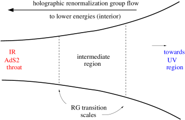
Figure 1: A cartoon of the bulk spacetime with
the holographic RG flow in the radial direction to
the infrared $AdS_{2}$ throat region from the far (UV)
region through possible intermediate regions (and
associated RG transition scales).

To prove the c-theorem for ${\cal C}$, we need to prove that ${\cal C}(u)$ decreases monotonically as we flow to lower energies $u$ (i.e. interior), or equivalently that ${\cal C}(u)$ is a monotonically increasing function as $u$ increases (outwards to the boundary). We will do this in two steps.

Step 1:  first define ${\tilde{\Phi}}=\Phi^{2/(D-2)}$. Then the first of the energy conditions (4) becomes

$${\tilde{\Phi}}=\Phi^{{2\over D-2}}\ ;\quad{\tilde{\Phi}}^{\prime\prime}={2\over D-2}\left({\Phi^{\prime\prime}\over\Phi}-{D-4\over D-2}{(\Phi^{\prime})^{2}\over\Phi^{2}}\right)\,\Phi^{{2\over D-2}}\quad\Rightarrow\quad-(D-2)\,B^{2}\,{{\tilde{\Phi}}^{\prime\prime}\over{\tilde{\Phi}}}\geq 0\ ,$$ (4.10)

so that ${\tilde{\Phi}}^{\prime}$ monotonically decreases as $u$ increases towards the boundary. In other words, ${\tilde{\Phi}}^{\prime}$ in the interior is larger than ${\tilde{\Phi}}^{\prime}$ near the boundary. If we can now argue that ${\tilde{\Phi}}^{\prime}$ is positive near the boundary, this would imply that ${\tilde{\Phi}}^{\prime}>0$ everywhere in the bulk as well. This then would imply that ${\tilde{\Phi}}(u)$ is a monotonically increasing function as $u$ increases and flows towards the boundary. A heuristic picture of the setup appears in Figure 1 (see also the discussion on nonconformal D2-branes, sec. 4.3, which exemplifies this).

Step 2:  Now we proceed to argue that ${\tilde{\Phi}}^{\prime}$ is positive near the boundary for suitable boundary conditions, namely that the ultraviolet of the theory belongs in the hvLif family (4.5) that we have been focussing on (which also includes $AdS$ for exponents $z=1,\theta=0$). The extremal branes we are considering here are excited states at finite charge density in these theories: the near boundary region corresponds to the high energy regime of the dual, well above the characteristic scales of the excited states. So it suffices to use the asymptotic (uncharged zero temperature) form of these backgrounds.

Using (4), we have $d_{i}=D-2$ and ${\tilde{\Phi}}=\Phi^{\frac{2}{d_{i}}}$. Then retaining only relevant factors, we have

$$\tilde{\Phi}\sim\Big{(}z-\frac{2\theta}{d_{i}}\Big{)}^{\frac{d_{i}-\theta}{zd_{i}-2\theta}}u^{\frac{d_{i}-\theta}{zd_{i}-2\theta}}\ ,\qquad\tilde{\Phi}^{\prime}\sim\Big{(}z-\frac{2\theta}{d_{i}}\Big{)}^{\frac{d_{i}-\theta}{zd_{i}-2\theta}}\frac{(d_{i}-\theta)}{(zd_{i}-2\theta)}\frac{1}{u^{\frac{d_{i}(z-1)-\theta}{zd_{i}-2\theta}}}\ ,$$

$$\tilde{\Phi}^{\prime\prime}\sim-\Big{(}z-\frac{2\theta}{d_{i}}\Big{)}^{\frac{d_{i}-\theta}{zd_{i}-2\theta}}\frac{(d_{i}-\theta)(d_{i}(z-1)-\theta)}{(zd_{i}-2\theta)^{2}}\frac{1}{u^{\frac{d_{i}(z-1)-\theta}{zd_{i}-2\theta}+1}}\ .$$ (4.11)

Then $\frac{\tilde{\Phi}^{\prime\prime}}{\tilde{\Phi}}\leq 0$ gives the null energy condition $(d_{i}-\theta)(d_{i}(z-1)-\theta)\geq 0$. A reasonable dual field theory requires positivity of specific heat if the theory is excited to finite temperature. Since the entropy for these theories scales as $S\sim V_{d_{i}}T^{d_{i}-\theta\over z}$, the positivity of the corresponding specific heat imposes ${d_{i}-\theta\over z}\geq 0$. This implies $d_{i}-\theta\geq 0$ since $z\geq 1$. Alongwith the null energy condition, this leads to $(d_{i}(z-1)-\theta)\geq 0$. These two conditions together imply

$$zd_{i}-2\theta=(d_{i}(z-1)-\theta)+(d_{i}-\theta)\geq 0\ .$$ (4.12)

Then we see that $\tilde{\Phi}^{\prime}$ is positive in this near boundary region. Roughly, ${\tilde{\Phi}}\sim u^{n}$ and ${\tilde{\Phi}}^{\prime}\geq 0$ and ${\tilde{\Phi}}^{\prime\prime}\leq 0$ require $n\geq 0$ and $n(n-1)\leq 0$, i.e. $0\leq n\leq 1$. We have argued that this is true if the null energy conditions and positivity of specific heat are satisfied.

Thus finally, we have shown that for the ultraviolet data we are considering, ${\tilde{\Phi}}(u)=\Phi^{2/(D-2)}$ is monotonically decreasing as $u$ flows to the interior (lower energies). Since the exponent ${2\over D-2}$ is positive, this implies that $\Phi(u)$ satisfies the same monotonicity property. This proves that the holographic c-function (4.9) we propose in fact satisfies the c-theorem.

At the IR $AdS_{2}$ horizon, ${\cal C}$ in (4.9) approaches the extremal black hole entropy (4.8), which is the IR number of degrees of freedom controlling the number of black hole microstates, akin to a central charge for this subsector. In fact it is this requirement that ${\cal C}\rightarrow S_{BH}$ at the IR $AdS_{2}$ fixed point which fixes the precise scaling of ${\cal C}$ in terms of $\Phi$ (else any positive power of $\Phi$ is monotonic, from the above arguments).

It is interesting to note that we have mainly used the first null energy condition in (4) in the above arguments. The second null energy condition appears to be more a condition on the matter configurations: for instance, the second condition for hvLif backgrounds (4.5) gives $z\geq 1,\ d_{i}+z-\theta\geq 0$ in 4.7), which follow from reality of the fluxes supporting the background, and also follows from specific heat positivity. to illustrate the condition in more generality, let us restrict to $D=4$ for simplicity: then the second condition in (4) gives

$$\frac{(\Phi^{2})^{\prime\prime}}{\Phi^{2}}\ \leq\ \frac{(B^{2})^{\prime\prime}}{B^{2}}\ ,$$ (4.13)

which says that the dilaton “acceleration” is not greater than that of the 2-dim metric. As we approach the $AdS_{2}$ region, we have $B^{2}\sim(u-u_{0})^{2}$ so this becomes $\frac{(\Phi^{2})^{\prime\prime}}{\Phi^{2}}\lesssim{2\over(u-u_{0})^{2}}$ which is trivially satisfied as $u\rightarrow u_{0}$ since the right hand side grows large. Thus the near $AdS_{2}$ region does not provide any additional constraint from this energy condition. However the near boundary region gives nontrivial constraints on the exponents defining the theory from this energy condition as we have seen. We will discuss this further later.

One might be concerned that the null energy conditions (and the Einstein equations) are second order equations while renormalization group flow is first order. It is important to note in this regard that the boundary conditions we have imposed is on the first derivative ${\tilde{\Phi}}^{\prime}$, which then automatically implies monotonicity. This physical boundary condition has effectively ruled out the other (growing) mode which would likely be singular in the interior.

In explicit examples (e.g. nonconformal branes redux, later), we can check this dilatonic c-function in fact has the right behaviour. Consider for instance an extremal brane in an hvLif theory where $B^{2},\Phi^{2}$ near the boundary have the form (4) while in the near $AdS_{2}$ region, $B^{2}\sim(u-u_{0})^{2}$ and $\Phi\sim u^{A}$ globally, with $A={d_{i}-\theta\over zd_{i}-2\theta}$ . Then using the arguments around (4.12), we see that $A\geq 0$ so that $\Phi^{2}(u)$ can be seen explicitly to monotonically decrease through the bulk as $u$ decreases flowing towards $AdS_{2}$. We also see that $A\leq 1$ so that $\Phi^{\prime\prime}\leq 0$ in accord with the first energy condition in (4). The second energy condition in the near boundary region simply imposes the constraints on the exponents that we have seen, which are required of the theory. In the near $AdS_{2}$ region, $B^{2}\sim(u-u_{0})^{2}$ and so as described above, the second energy condition is satisfied. This family includes $AdS$ where $z=1,\theta=0$ and $\Phi^{2}=u^{2}$.

From the point of dual 1-dim theories which flow to the $CFT_{1}$ dual to the $AdS_{2}$ bulk theory, the arguments above suggest that ${\cal C}$ in (4.9) is a candidate c-function. While spatial coarse-graining does not make sense in $0+1$-dim (no space!), the renormalization group defined in terms of integrating out high energy modes does make sense, i.e. as a flow to lower energies (IR). In the present context, we have defined the holographic c-function ${\cal C}$ as essentially inherited from the higher dimensional theory that has been compactified: it would be interesting to understand the c-function from the dual 1-dim point of view.

4.2 Null energy conditions from the $2$-dim perspective

We have described the null energy conditions $T_{\mu\nu}n^{\mu}n^{\nu}\geq 0$ in the higher dimensional theory and recast them in terms of 2-dim bulk variables $g^{(2)}_{\mu\nu},\ \Phi$. The two independent null vectors give two independent null energy conditions (4) as we have seen. However it is interesting to note that only one of the null vectors — $\zeta^{M}=(\sqrt{-g^{tt}},\sqrt{g^{uu}})$ — has a natural interpretation intrinsically in the 2-dimensional spacetime. This leads to the first of the energy conditions. The second one appears to have no intrinsic interpretation directly in 2-dimensions: however we can reverse engineer this from the higher dimensional theory and recast it in terms of the potential governing the dilaton and other scalars in the context of the dilaton-gravity-scalar theory (3.4).

The $tr-$ and $ii$-components, for $i=1,\dots,D-2$, of Einstein equations for the gravity-scalar action in $D$-dimensions (3.1) are

$$\mathcal{R}^{(D)}_{\mu\nu}-\frac{g^{(D)}_{\mu\nu}}{2}\mathcal{R}^{(D)}=\frac{h_{IJ}}{2}\Big{(}\partial_{\mu}\Psi^{I}\partial_{\nu}\Psi^{J}-\frac{g^{(D)}_{\mu\nu}}{2}\partial_{M}\Psi^{I}\partial^{M}\Psi^{J}\Big{)}-\frac{g^{(D)}_{\mu\nu}}{2}V\ ,$$ (4.14)

$$\mathcal{R}^{(D)}_{ii}-\frac{g^{(D)}_{ii}}{2}\mathcal{R}^{(D)}=\frac{h_{IJ}}{2}\Big{(}\partial_{i}\Psi^{I}\partial_{i}\Psi^{J}-\frac{g^{(D)}_{ii}}{2}\partial_{M}\Psi^{I}\partial^{M}\Psi^{J}\Big{)}-\frac{g^{(D)}_{ii}}{2}V+\frac{\partial V}{\partial g^{(D)\,ii}}\ ,$$ (4.15)

where we have taken the metric to be diagonal in the spatial components i.e. $g^{(D)}_{ij}=0\ \forall\ i\neq j$ and the potential $V$ in (3.1) to be dependent only on $g^{(D)}_{ii}$ components. These equations $G^{(D)}_{MN}=8\pi G_{D}T^{(D)}_{MN}$ give the stress tensor components as

$$8\pi G_{D}T^{(D)}_{\mu\nu}=\frac{h_{IJ}}{2}\Big{(}\partial_{\mu}\Psi^{I}\partial_{\nu}\Psi^{J}-\frac{g^{(D)}_{\mu\nu}}{2}\partial_{M}\Psi^{I}\partial^{M}\Psi^{J}\Big{)}-\frac{g^{(D)}_{\mu\nu}}{2}V\ ,$$ (4.16)

$$8\pi G_{D}T^{(D)}_{xx}=\frac{h_{IJ}}{2}\Big{(}\partial_{x}\Psi^{I}\partial_{x}\Psi^{J}-\frac{g^{(D)}_{xx}}{2}\partial_{M}\Psi^{I}\partial^{M}\Psi^{J}\Big{)}-\frac{g^{(D)}_{xx}}{2}V+\frac{\partial\,V}{\partial g^{(D)\,xx}}\ .\qquad$$ (4.17)

After dimensional reduction, we obtain the 2-dim action (3.4) and the above equations become the 2-dim Einstein equations and the dilaton equation in (3). In particular the higher dimensional $\mu\nu$-components give 2-dim Einstein equations which we write in the form

$$\frac{1}{\Phi^{2}}[g_{\mu\nu}\nabla^{2}\Phi^{2}-\nabla_{\mu}\nabla_{\nu}\Phi^{2}]=8\pi G_{D}T^{(D)}_{\mu\nu}\ ,$$

$$8\pi G_{D}T^{(D)}_{\mu\nu}=\frac{h_{IJ}}{2}\Big{(}\partial_{\mu}\Psi^{I}\partial_{\nu}\Psi^{J}-\frac{g_{\mu\nu}}{2}\partial_{M}\Psi^{I}\partial^{M}\Psi^{J}\Big{)}-\frac{g_{\mu\nu}U}{2\Phi^{2}}\ .$$ (4.18)

The $xx$-component of the higher dimensional stress tensor can likewise be expressed in terms of the 2-dim potential and its derivative as

$$8\pi G_{D}T^{(D)}_{xx}=-\frac{\Phi^{\frac{4}{(D-2)}}}{4}h_{IJ}\partial_{M}\Psi^{I}\partial^{M}\Psi^{J}-\frac{(D-2)}{2}\Phi^{\frac{2}{D-2}+2}\,\frac{\partial U}{\partial\Phi^{2}}\ .$$ (4.19)

This has no obvious 2-dim origin intrinsically: the null energy condition intrinsic to two dimensions involves only $T_{\mu\nu}$ but not $T_{xx}$. Further the null vector $\xi^{M}$ in (4.3) has no intrinsically 2-dimensional meaning. The second null energy condition in (4) from the higher dimensional theory can however be recast in 2-dimensional language in terms of the stress tensor components above and it is then interesting to ask what 2-dimensional constraints it leads to. This second NEC $T^{(D)}_{MN}\xi^{M}\xi^{N}\geq 0$ for the null vector

$$\xi^{M}=(\sqrt{-g^{(D)\,tt}},0,\sqrt{g^{(D)\,xx}},0,\ldots,0)=(\sqrt{-g^{tt}}\Phi^{\frac{D-3}{D-2}},0,\Phi^{\frac{-2}{D-2}},0,\dots,0)$$ (4.20)

becomes

$$8\pi G_{D}(T^{(D)}_{tt}(\xi^{t})^{2}+T^{(D)}_{xx}(\xi^{x})^{2})=-\Phi^{\frac{2(D-3)}{(D-2)}}\frac{g^{tt}h_{IJ}}{2}\partial_{t}\Psi^{I}\partial_{t}\Psi^{J}+\frac{\Phi^{\frac{-2}{D-2}}}{2}\Big{(}U-(D-2)\Phi^{2}\frac{\partial U}{\partial\Phi^{2}}\Big{)}\geq 0\ .$$ (4.21)

For static backgrounds as we have here, $\partial_{t}\Psi^{I}=0$: then this second NEC becomes a nontrivial condition on the potential and its derivative

$$U-(D-2)\,\Phi^{2}\,\frac{\partial U}{\partial\Phi^{2}}\ \geq\ 0\ .$$ (4.22)

In 2-dim dilaton-gravity-matter theories that arise from some higher dimensional reduction, this condition (4.22) is simply recognized as the second NEC in (4). However if we regard (3.4) as an intrinsically 2-dim theory, then it appears reasonable to impose such a constraint on the dilaton-matter potential.

To illustrate this, consider first a potential of a form we have seen arising from reduction of 4-dim Einstein-Maxwell theory,

$$U=-V_{0}\Phi+{V_{2}\over\Phi^{3}}\qquad\Rightarrow\qquad U-2\Phi^{2}{dU\over d\Phi^{2}}={4V_{2}\over\Phi^{4}}\geq 0\quad\Rightarrow\quad V_{2}\geq 0\ .$$ (4.23)

Of course this can be recognized as the condition $Q^{2}\geq 0$ in the higher dimensional theory: from the 2-dim point of view, the condition gives positivity constraints on the coefficients that appear in the potential.

The first NEC in $D$-dimensions, $T^{(D)}_{MN}\zeta^{M}\zeta^{N}\geq 0$, or $\mathcal{R}^{(D)}_{MN}\zeta^{M}\zeta^{N}\geq 0$ for the null vector $\zeta^{M}=(\sqrt{-g^{(D)\,tt}},\sqrt{g^{(D)\,rr}},0,0,\dots,0)=(\sqrt{-g^{tt}}\Phi^{\frac{D-3}{D-2}},\sqrt{g^{rr}}\Phi^{\frac{D-3}{D-2}},0,0,\dots,0)$  becomes the 2-dim NEC $\mathcal{R}_{\mu\nu}\tilde{\zeta}^{\mu}\tilde{\zeta}^{\nu}\geq 0$ for the 2-dim null vector $\tilde{\zeta}^{\mu}=(\sqrt{-g^{tt}},\sqrt{g^{rr}})$. Using (4.2), this NEC gives

$$-\nabla_{\mu}\nabla_{\nu}\Phi^{2}\tilde{\zeta}^{\mu}\tilde{\zeta}^{\nu}=g^{tt}\nabla_{t}\nabla_{t}\Phi^{2}-g^{rr}\nabla_{r}\nabla_{r}\Phi^{2}\geq 0\ .$$ (4.24)

For static backgrounds, this recovers the condition on the “acceleration” of the dilaton that we have studied earlier in the context of the c-theorem.

4.3 The c-function in the $M2$-$D2$ system

Nonconformal $Dp$-branes upon dimensional reduction on the transverse sphere give rise to hvLif theories with $z=1$ and nonzero $\theta$ [55]. In particular the $D2$-brane supergravity phase upon $S^{6}$-reduction give rise to bulk 4-dim hvLif theories with $z=1,\ \theta=-{1\over 3}$ . These flow [56] in the infrared to M2-branes, which give rise to $AdS_{4}$ upon $S^{7}$-reduction (with $z=1,\theta=0$). These are all uncharged phases. Adding a $U(1)$ gauge field to this system — which can be taken as the dual to the $U(1)_{R}$ current — and tuning to extremality gives string realizations for the extremal versions of the above 4-dim theories. We have in mind that the $AdS_{4}$ phase eventually terminates in the deep IR at an $AdS_{2}$ throat: see Figure 1. Since the transition from the D2-phase to the M2-$AdS_{4}$ phase occurs at energies well above the IR scale where the $AdS_{2}$ emerges, the D2-phase can be essentially regarded as uncharged for the purposes of the discussion below. In the far UV, the D2-branes are described by free 3-dim SYM.

The string frame metric and the dilaton describing $N$ $D2$-branes are

$$ds_{st}^{2}=\frac{r^{5/2}}{R_{2}^{5/2}}dx_{||}^{2}+\frac{R_{2}^{5/2}}{r^{5/2}}dr^{2}+\frac{R_{2}^{5/2}}{r^{1/2}}d\Omega_{6}^{2}\ ,\qquad e^{\phi}=g_{s}\Big{(}\frac{R_{2}^{5}}{r^{5}}\Big{)}^{1/4}\ ,$$ (4.25)

with $e^{\phi_{\infty}}=g_{s}$ the asymptotic value of the dilaton, and

$$g_{YM}^{2}=\frac{g_{s}}{\sqrt{\alpha^{\prime}}}\ ,\qquad R_{2}^{5}=\alpha^{\prime 3}g_{YM}^{2}N\ ,$$ (4.26)

where we are ignoring numerical factors (since we will be primarily interested here in the scaling behaviour along the RG flow). The 10-dim Einstein frame metric $ds_{E}^{2}=e^{-\frac{1}{2}(\phi-\phi_{\infty})}ds_{st}^{2}$ after dimensional reduction on $S^{6}$ gives the Einstein metric of the effective 4-dim hvLif theory with $d_{i}=2$, $z=1$, $\theta=-\frac{1}{3}$,

$$ds^{2}=\frac{r^{7/2}}{R_{2}^{7/2}}(-dt^{2}+dx_{1}^{2}+dx_{2}^{2})+\frac{R_{2}^{3/2}}{r^{3/2}}dr^{2}=\Big{(}\frac{\rho}{R_{2}}\Big{)}^{1/3}\Big{[}\frac{\rho^{2}}{R_{2}^{2}}(-dt^{2}+dx_{i}^{2})+\frac{R_{2}^{2}}{\rho^{2}}d\rho^{2}\Big{]}\ .$$ (4.27)

The second expression is written in coordinates where the hvLif form (4.5) is manifest. We have

$$\rho=\frac{r^{3/2}}{R_{2}^{1/2}}\ ,\qquad w=\frac{r^{3/2}}{R_{2}^{5/2}}\ ,\qquad u={r^{2}\over R_{2}}\ ,$$ (4.28)

where $w={r^{(5-p)/2}\over R_{p}^{(7-p)/2}}$ is the nonconformal $Dp$-brane supergravity radius/energy variable introduced in [24]. This coordinate has also proved useful in studies of entanglement entropy and its interpretation in the nonconformal brane system [57, 58]. The coordinate $u$ is chosen to cast the metric above in the form (4.1) that we found useful in analysing the c-function in our earlier discussion: in terms of those expressions, we have

$$B^{2}={r^{7/2}\over R_{2}^{7/2}}={u^{7/4}\over R_{2}^{7/4}}\ ,\qquad\Phi^{2}={r^{7/2}\over R_{2}^{7/2}}=w^{7/3}\,R_{2}^{7/3}\ .$$ (4.29)

Then the c-function (4.9) written in terms of the energy variable $w$ in the D2-phase is

$${\cal C}(w)\sim{V_{2}\Phi^{2}\over G_{4}}=V_{2}\,w^{7/3}\,N^{2}{1\over(g_{YM}^{2}N)^{1/3}}\ =\ V_{2}\,w^{2}\,N_{eff}(w)\ ,$$ (4.30)

after spatial compactification of the D2-branes. Here we have used

$$G_{4}\sim\frac{G_{10}}{Vol(S^{6})}\sim\frac{g_{s}^{2}\alpha^{\prime 4}}{R_{2}^{6}}\ ,\qquad N_{eff}(w)=N^{2}{1\over(g_{YM}^{2}N/w)^{1/3}}\ ,$$ (4.31)

and $N_{eff}(w)$ is the scale-dependent number of degrees of freedom for the D2-phase (which also has played useful roles in entanglement studies [57, 58]), while the dimensionless gauge coupling at scale $w$ is $g_{eff}={g_{YM}^{2}N\over w^{3-p}}$ .

The M2-phase is given by the $AdS_{4}\times S^{7}$ background (again ignoring numerical factors)

$$ds^{2}={r^{2}\over R^{2}}dx_{||}^{2}+{R^{2}\over r^{2}}dr^{2}+R^{2}d\Omega_{7}^{2}\ ,\qquad R^{6}\sim Nl_{p}^{6}\ ,\qquad G_{4}\sim\frac{G_{11}}{Vol(S^{7})}\sim\frac{l_{p}^{9}}{R^{7}}\ ,$$ (4.32)

which after reducing on the $S^{7}$ gives $AdS_{4}$ (and $l_{p}$ is the 11-dim Planck length; note that $R^{6}\sim Nl_{P}^{6}\sim g_{s}R_{2}^{5}\sqrt{\alpha^{\prime}}$). This is already in the form (4.1) with $u=r$ and the energy variable $w={r\over R^{2}}$ and $\Phi^{2}={r^{2}\over R^{2}}$ . Then the c-function in this M2-phase after spatial compactification is

$${\cal C}(w)={V_{2}\over G_{4}}\,{r^{2}\over R^{2}}={R^{2}\over G_{4}}\,V_{2}\,w^{2}=N^{3/2}\,V_{2}\,w^{2}\ ,$$ (4.33)

using ${R^{2}\over G_{4}}={R^{9}\over G_{11}}=N^{3/2}$. It is useful to recall [56] that the D2-phase is valid in the regime $g_{YM}^{2}N^{1/5}\ll{r\over\alpha^{\prime}}\ll g_{YM}^{2}N$ so that $N^{3/2}\ll N_{eff}(w)\ll N^{2}$. At the scale ${r\over\alpha^{\prime}}\sim g_{YM}^{2}$ the system transits from a smeared (arrayed) M2-phase to the M2-$AdS_{4}$ phase. At this scale which corresponds to $w\sim g_{YM}^{2}N^{-1/2}$, we have $N_{eff}(w)\sim N^{3/2}$  and the D2-phase c-function can be seen to match that in the M2-phase. The present analysis cannot be applied to the intermediate interpolating phase corresponding to smeared (arrayed) M2-branes.

We have so far discussed uncharged D2-M2 phases. With the $AdS_{2}$ emerging in the deep IR (within the $AdS_{4}$ region), the transition between the D2- and M2-phase is well approximated by the uncharged system. To see this explicitly, note that the charged hvLif metric arising from D2-redux is

$$ds^{2} = \Big{(}\frac{\rho}{R_{2}}\Big{)}^{1/3}\Big{[}\frac{\rho^{2}}{R_{2}^{2}}(-f(\rho)dt^{2}+dx_{1}^{2}+dx_{2}^{2})+\frac{R_{2}^{2}}{\rho^{2}f(\rho)}d\rho^{2}\Big{]}\ ,$$

$$f(\rho) = 1-\Big{(}\frac{\rho_{0}}{\rho}\Big{)}^{10/3}+\frac{Q_{D}^{2}}{\rho^{14/3}}\Big{(}1-\Big{(}\frac{\rho}{\rho_{0}}\Big{)}^{4/3}\Big{)}\ .$$ (4.34)

with $Q_{D}^{2}\sim\rho_{0}^{7/3}$ at extremality. Since the transition is occurring at a scale $\rho_{trans}\gg\rho_{0}$, we essentially have $f(\rho)\sim 1$ in that region. In the deep IR, the extremal M2-$AdS_{4}$ phase

$$ds^{2}={r^{2}\over R^{2}}(-f(r)dt^{2}+dx_{i}^{2})+{R^{2}\over r^{2}f(r)}dr^{2}\ ,\qquad f(r)=1-\Big{(}\frac{r_{0}}{r}\Big{)}^{3}+\frac{Q^{2}}{r^{4}}\Big{(}1-\frac{r}{r_{0}}\Big{)}\ ,$$ (4.35)

(after $S^{7}$ reduction) with $Q^{2}\sim r_{0}^{4}$ develops an $AdS_{2}$ throat, with the horizon at $r=r_{0}$. Then the IR scale at the horizon is $u={r_{0}\over R^{2}}$ and the c-function approaches

$${\cal C}\ \xrightarrow{\ AdS_{2}\ }\ N^{3/2}\,{V_{2}\,Q\over R^{4}}\ .$$ (4.36)

This phase is dual to a doped $CFT_{3}$, with dopant density $\sigma_{Q}\equiv{Q\over R^{4}}$ which is essentially the number of dopant charge carriers per unit area of the M2-branes: then ${\cal C}_{IR}$ is essentially a “central charge” whose $N^{3/2}$ scaling reflects the underlying number of degrees of freedom of the M2-$CFT$, which has been doped with an additional $V_{2}\sigma_{Q}$ number of charge carriers distributed over the volume $V_{2}$ of the M2-branes (there are some parallels with the heuristic partonic picture of entanglement for excited $AdS$ plane wave states in [59]). This “central charge” corresponds to the number of microstates of the doped $CFT_{1}$ obtained by spatial compactification of the M2-branes: it is essentially dual to the $AdS_{2}$ theory describing the extremal black brane with $C_{IR}$ the extremal entropy. In some sense, $w^{2}={Q(w)\over R^{4}}$ is a scale-dependent dopant density with $w_{IR}^{2}={Q\over R^{4}}$ the infrared value. String/M-theory realizations of this involve turning on an appropriate $G_{4}$-flux in the M2-brane system which after the $S^{7}$ reduction gives the additional $U(1)$ gauge field that provides charge [60].

It is clear that the c-function (4.30) in the D2-phase gives a larger number of degrees of freedom than that in the M2-phase (4.33) (noting the regimes for $w$, which flows to lower energies), in accord with our general discussions of the c-function earlier. This dovetails with the fact that $\theta$ is negative in the D2-phase (with $z=1$). It is also worth noting that the precise $N$-scalings etc arise from the precise dimensionful factors contained in the dilaton.

4.4 c-function in the $M5$-$D4$ system

The M5-D4 brane system flows from an $AdS_{7}\times S^{4}$ phase (dual to the 6-dim $(2,0)$ theory) through the D4-supergravity phase to finally 5-dim SYM in the IR. While this does not admit an $AdS_{2}$ region in the deep IR of the phase diagram, it is interesting to study the c-function (4.9) in this case as well. This discussion has parallels with the D2-M2 case so we will be succinct. For the $M5$-$AdS_{7}$ phase, we have

$$ds^{2}={r^{2}\over R^{2}}dx_{||}^{2}+{R^{2}\over r^{2}}dr^{2}+R^{2}d\Omega_{4}^{2}\ ,\qquad R^{3}\sim Nl_{p}^{3}\ ,\qquad G_{7}\sim\frac{G_{11}}{Vol(S^{4})}\sim\frac{l_{p}^{9}}{R^{4}}\ ,$$ (4.37)

which after reducing on the $S^{4}$ gives $AdS_{7}$ ($l_{p}$ is the 11-dim Planck length). This dovetails with (4.1) with $u=r$ and the energy variable $w={r\over R^{2}}$ and $\Phi^{2}={r^{2}\over R^{2}}$ . The c-function in this M5-phase after spatial $T^{5}$-compactification then is

$${\cal C}(w)_{M5}={V_{5}\over G_{7}}\,{r^{2}\over R^{2}}={R^{5}\over G_{7}}\,V_{5}\,w^{5}=N^{3}\,V_{5}\,w^{5}\ ,$$ (4.38)

using ${R^{5}\over G_{7}}\sim{R^{9}\over G_{11}}\sim N^{3}$ here. Now for the $N$ $D4$-branes phase, the string metric and dilaton are

$$ds_{st}^{2}=\frac{r^{3/2}}{R_{4}^{3/2}}dx_{||}^{2}+\frac{R_{2}^{3/2}}{r^{3/2}}dr^{2}+R_{2}^{3/2}\,r^{1/2}d\Omega_{4}^{2}\ , e^{\phi}=g_{s}\Big{(}\frac{r}{R_{4}}\Big{)}^{3/4}\ ,$$

$$g_{YM}^{2}\sim g_{s}\sqrt{\alpha^{\prime}}, \ R_{4}^{3}\sim\alpha^{\prime}g_{YM}^{2}N\ ,$$ (4.39)

ignoring numerical factors. The 10-dim Einstein frame metric $ds_{E}^{2}=e^{-\frac{1}{2}(\phi-\phi_{\infty})}ds_{st}^{2}$ after $S^{4}$-redux gives a 6-dim hvLif theory (4.5) with $d_{i}=4$, $z=1$, $\theta=-1$,

$$ds^{2}=\frac{r^{5/4}}{R_{4}^{5/4}}\Big{(}-dt^{2}+\sum_{i=1}^{4}dx_{i}^{2}\Big{)}+\frac{R_{4}^{7/4}}{r^{7/4}}dr^{2}=\Big{(}\frac{\rho}{R_{4}}\Big{)}^{1/2}\Big{[}\frac{\rho^{2}}{R_{4}^{2}}(-dt^{2}+\sum_{i=1}^{4}dx_{i}^{2})+\frac{R_{4}^{2}}{\rho^{2}}d\rho^{2}\Big{]}.\ \$$ (4.40)

The D4-brane supergravity radius/energy variable $w$ [24] and the $u$ coordinate in (4.1) are

$$\rho=R_{4}^{1/2}r^{1/2}\ ,\qquad w=\frac{r^{1/2}}{R_{4}^{3/2}}\ ,\qquad u={r^{3/2}\over R_{4}^{1/2}}\ .$$ (4.41)

With $G_{6}\sim G_{10}/Vol(S^{4})\sim g_{s}^{2}\alpha^{\prime 4}/R_{4}^{4}$,  the scale-dependent number of degrees of freedom $N_{eff}(w)$ for the D4-phase [57, 58], and the dilaton $\Phi^{2}=g_{xx}^{(D-2)/2}={r^{5/2}\over R_{4}^{5/2}}$, the c-function (4.9) is

$${\cal C}(w)_{D4}={V_{4}\Phi^{2}(w)\over 4G_{6}}\sim V_{4}\,w^{4}\,N_{eff}(w)\ ,\qquad N_{eff}(w)=N^{2}(g_{YM}^{2}Nw)\ ,$$ (4.42)

after spatial $T^{4}$-compactification, and the regime of validity is $1\ll g_{YM}^{2}Nw\ll N^{2/3}$ . Noting $R_{11}=g_{s}\sqrt{\alpha^{\prime}}\sim g_{YM}^{2}$ and $V_{5}=V_{4}R_{11}$, we see that the c-function continuously transits from the M5- to the D4-phase for length scales longer than the 11th circle size $R_{11}$. This leads to the guess that the c-function in the free 5-dim SYM phase after spatial $T^{4}$-compactification is possibly $N^{2}V_{4}w^{4}$.

4.5 On dilatonic and entropic c-functions

It is interesting to compare the dilatonic c-function we have defined with the entropic c-function [61, 62] that has been studied based on studies of entanglement entropy [63, 64, 65, 66].

Consider the bulk geometry (4.1) with asymptotics being $AdS$ or hvLif, focussing on $D=4$ dimensions (with no compactification). For a strip subsystem with width along say $x$, the induced metric on a time slice is $\Phi^{2}dy^{2}+{du^{2}\over B^{2}}+\Phi^{2}dx^{2}$ and the area functional for holographic entanglement [67] is $A=L\int du\,{\Phi\over B}\sqrt{1+B^{2}\Phi^{2}\,({dx\over du})^{2}}$ which after extremization gives

$$S={2L\over 4G_{4}}\int{du\over B}{\Phi^{3}\over\sqrt{\Phi^{4}-\Phi_{*}^{4}}}\ ,\qquad l=\int{du\over B}{\Phi_{*}^{2}\over\Phi\sqrt{\Phi^{4}-\Phi_{*}^{4}}}\ ,$$ (4.43)

where $\Phi_{*}=\Phi(u_{*})$ is the value of the dilaton at the turning point $u_{*}$ of the minimal surface, and $L$ is the size of the (essentially infinitely long) strip in the longitudinal $y$ direction. For instance, for a strip in $AdS_{4}$, the area and width integrals are $S={2L\over 4G_{4}}\int_{\epsilon}^{u_{*}}{Rdu\over u}{u^{3}\over\sqrt{u^{4}-u_{*}^{4}}}\sim{R^{4}\over G_{4}}({L\over\epsilon}-{L\over l})$ and $l\sim{R^{2}\over u_{*}}$ . The entropic c-function is then defined as

$$c_{E}={l^{2}\over L}{dS\over dl}\ ,$$ (4.44)

which gives $c_{E}\sim{R^{2}\over G_{4}}$ . This is thus a measure of the local number of degrees of freedom, or central charge, in the dual field theory responsible for entanglement. In theories with an RG flow, the entropic c-function is scale dependent and satisfies ${dc_{E}\over dl}\leq 0$, i.e. it monotonically decreases with the width $l$, and thus plays the role of a c-function based on entanglement entropy. For instance for nonconformal branes, $c_{E}(l)\sim N_{eff}(l)$.

We will now try to draw comparisons between this entropic c-function and the dilatonic c-function (4.9). Away from the $AdS_{2}$ horizon, $u\gg u_{0}$ and we have $B\sim{u-u_{0}\over R}\sim{u\over R}$ . Since the dilaton monotonically decreases flowing towards the interior, i.e. as $u$ decreases in (4.1), we can recast the integrals above as

$$S={2L\over 4G_{4}}\,\Phi_{*}\,R\int_{\varphi_{\epsilon}}^{1}{du\over u}{\varphi^{3}\over\sqrt{\varphi^{4}-1}}\ ,\qquad l={2R\over\Phi_{*}}\int_{\varphi_{\epsilon}}^{1}{du\over u}{1\over\varphi\sqrt{\varphi^{4}-1}}\ ,\qquad\varphi={\Phi\over\Phi_{*}}\ .$$ (4.45)

Since the dilaton decreases monotonically, we can redefine the radial variable by $\varphi$ as $du={d\varphi\over\varphi^{\prime}}$ , and we note that all the information about the turning point has been scaled out after this recasting to the factors outside the integrals. The entropic c-function receives a nonvanishing contribution simply from the finite part for which the integrals are simply finite numerical factors. Then we see that $S\sim{R\over G_{4}}\Phi_{*}L\sim{R^{2}\over G_{4}}\,{L\over l}$ which recovers $c_{E}\sim{R^{2}\over G_{4}}$ .

From the discussion of the c-function for M2-branes (4.33), we see that ${\cal C}(w)=N^{3/2}V_{2}w^{2}$. Recalling that ${R^{2}\over G_{4}}\sim N^{3/2}$, we see that the dilatonic c-function scales as the entropic number of degrees of freedom (i.e. $c_{E}$), but is in addition extensive: it scales with $V_{2}$ and shrinks as $w^{2}$ along the flow to the IR. In the 2-dim bulk theory after compactification, $c_{E}$ cannot be formulated since the spatial directions are compactified but the dilatonic c-function nevertheless encodes the number of degrees of freedom that $c_{E}$ encodes. Similar comparisons can be drawn for other cases.

It is also interesting to recall the holographic c-function in [29]. For a bulk theory $ds^{2}=e^{2A(\varrho)}dx_{\parallel}^{2}+d\varrho^{2}$ enjoying Lorentz invariance (i.e. $z=1$), this c-function is $C_{FGPW}(w)\sim{1\over G_{D}\,(dA/d\varrho)^{d_{i}}}$ where $d_{i}$ is the number of boundary spatial dimensions. For $AdS_{D}$, we have $A\sim\log{\varrho\over R}$ and $c_{FGPW}\sim{R^{d_{i}}\over G_{D}}$ which gives $c_{FGPW}\sim N^{3/2}$ for M2-$AdS_{4}$. For nonconformal $Dp$-branes ($g_{YM}^{2}\sim g_{s}{\alpha^{\prime}}^{(p-3)/2}$) [56]

$$ds^{2}_{st}={r^{(7-p)/2}\over R_{p}^{(7-p)/2}}dx_{\parallel}^{2}+{R_{p}^{(7-p)/2}\over r^{(7-p)/2}}(dr^{2}+r^{2}d\Omega_{8-p}^{2}),\quad e^{\Phi}=g_{s}\Big{(}{R_{p}^{7-p}\over r^{7-p}}\Big{)}^{{3-p\over 4}},\ \ \ R_{p}^{7-p}\sim g_{YM}^{2}N{\alpha^{\prime}}^{5-p},$$ (4.46)

upon $S^{8-p}$-redux give the hvLif metric (4.5) with $z=1,\ p=d_{i}$ [55]: in this case, using

$$\theta=p-{9-p\over 5-p}=-{(p-3)^{2}\over 5-p}\ ,\quad ds_{p+2}^{2}=\Big{(}{\varrho\over R_{p}}\Big{)}^{2\left(1-{d_{i}\over\theta}\right)}dx_{\parallel}^{2}+d\varrho^{2}\ ,\quad{\varrho\over R_{p}}=\Big{(}{r\over R_{p}}\Big{)}^{-{\theta(5-d_{i})\over 2d_{i}}},$$ (4.47)

we see that the dilatonic c-function (4.9) we have discussed (after redux to 2-dim) gives

$${\cal C}(w)\sim N_{eff}(w)V_{d_{i}}w^{d_{i}}\ ,\qquad N_{eff}(w)=N^{2}\left({g_{YM}^{2}N\over w^{3-p}}\right)^{p-3\over 5-p},\quad w={r^{(5-p)/2}\over R_{p}^{(7-p)/2}}\ ,$$ (4.48)

as we have seen earlier in the detailed discussions on the D2-M2 and M5-D4 phases (with $w$ the nonconformal $Dp$-brane supergravity radius/energy variable [24]). On the other hand, the c-function in [29] mentioned above can be seen to be $c_{FGPW}\sim N_{eff}(w)$, with the same scaling as the entropic c-function $c_{E}$: this is a measure of the local degrees of freedom of the higher dimensional theory, while the dilatonic c-function ${\cal C}$ has additional extensivity arising from the compactification.

5 2-dim radial Hamiltonian formalism and $\beta$-functions

A version of the holographic renormalization group was formulated in [25]: using a radial ADM-type split of the bulk spacetime, the radial Hamiltonian constraint gives rise to flow equations for couplings and corresponding $\beta$-functions. This is not a Wilsonian formulation since the effective action at the scale corresponding to some radial slice depends on data not just at higher energy scales that have been integrated out: Wilsonian formulations of the holographic renormalization group have been investigated in [33, 34]. Nevertheless this dVV formulation gives useful qualitative insights into the holographic renormalization group. In this section, we will adapt this to obtain renormalization group flow equations and $\beta$-functions starting with the 2-dim dilaton-gravity-scalar theory. As in [25], writing the boundary 1-dim action on some radial slice in a radial Hamilton-Jacobi formulation, we separate this at low scales into local and nonlocal parts and then write the local part in a derivative expansion. Taking the leading term to arise from just a “boundary potential” term for the couplings (scalars $\Phi,\Psi^{I}$), i.e. no derivatives, we obtain relations between the original potential and the boundary potential using the Hamiltonian constraint, thereby obtaining $\beta$-functions from the flow equations. We will describe this below.

Consider the 2-dim gravity-scalar action (3.4) including the Gibbons-Hawking term

$$S=\frac{1}{16\pi G_{2}}\int d^{2}x\sqrt{-g}\Big{(}\Phi^{2}\mathcal{R}-\frac{\Phi^{2}}{2}h_{IJ}\partial_{\mu}\Psi^{I}\partial^{\mu}\Psi^{J}-U(\Phi,\Psi^{I})\Big{)}+\frac{1}{16\pi G_{2}}\int dt\sqrt{-\gamma}\Phi^{2}2K\ ,$$ (5.1)

where $U(\Phi,\Psi^{I})=V\Phi^{\frac{2}{D-2}}$ . Substituting the radial decomposition of the metric

$$ds^{2}=(N^{2}+\gamma_{tt}(N^{t})^{2})dr^{2}+2\gamma_{tt}N^{t}dtdr+\gamma_{tt}dt^{2}\ ,$$ (5.2)

certain boundary terms cancel with the Gibbons-Hawking term: then massaging leads to a radial Lagrangian (in Appendix B, we derive this from dimensional reduction of the Hamiltonian formulation of a higher dimensional theory of the sort we have been considering)

$$L=\frac{1}{16\pi G_{2}}\int dt\sqrt{-\gamma}\,N\,\Big{[}-2\Box_{t}\Phi^{2}+\frac{2K}{N}(\partial_{r}\Phi^{2}-N^{t}\partial_{t}\Phi^{2})-\frac{\Phi^{2}}{2}h_{IJ}\partial_{\mu}\Psi^{I}\partial^{\mu}\Psi^{J}-U\Big{]}\ ,$$ (5.3)

where the extrinsic curvature and the covariant derivative w.r.t. $\gamma_{tt}$ are

$$K_{tt}=\frac{1}{2N}(\partial_{r}\gamma_{tt}-2D_{t}N_{t})\ ,\quad K=\gamma^{tt}K_{tt}\ ,\quad D_{t}N_{t}=\partial_{t}N_{t}-\Gamma^{t}_{tt}N_{t}\ ,\quad\Box_{t}\equiv\gamma^{tt}D_{t}D_{t}\ ,$$ (5.4)

where $\gamma^{tt}=(\gamma_{tt})^{-1}$ and $N_{t}=\gamma_{tt}N^{t}$. The conjugate momenta for the fields $\gamma_{tt}$, $\Phi$ and $\Psi^{I}$ are

$$\pi^{tt}\equiv\frac{16\pi G_{2}}{\sqrt{-\gamma}}\frac{\delta L}{\delta\dot{\gamma}_{tt}}=\frac{\gamma^{tt}}{N}(\partial_{r}\Phi^{2}-N^{t}\partial_{t}\Phi^{2})\ ,$$

$$\pi_{\Phi}\equiv\frac{16\pi G_{2}}{\sqrt{-\gamma}}\frac{\delta L}{\delta\dot{\Phi}}=4K\Phi=\frac{2\Phi\gamma^{tt}}{N}(\dot{\gamma}_{tt}-2D_{t}N_{t})\ ,$$

$$\pi_{I}\equiv\frac{16\pi G_{2}}{\sqrt{-\gamma}}\frac{\delta L}{\delta\dot{\Psi}^{I}}=-\frac{\Phi^{2}h_{IJ}}{N}(\dot{\Psi}^{J}-N^{t}\partial_{t}\Psi^{J})\ ,$$ (5.5)

where dot represents the radial derivative,i.e. $\dot{\Phi}=\partial_{r}\Phi$ and so on. Inverting, we obtain

$$\dot{\Phi}=\frac{1}{2\Phi}\Big{(}\frac{N\pi^{tt}}{\gamma^{tt}}+N^{t}\partial_{t}\Phi^{2}\Big{)}\ ,$$

$$\dot{\gamma}_{tt}=\frac{N\pi_{\Phi}}{2\Phi\gamma^{tt}}+2D_{t}N_{t}\ ,$$

$$\dot{\Psi}^{I}=-\frac{Nh^{IJ}\pi_{J}}{\Phi^{2}}+N^{t}\partial_{t}\Psi^{I}\ .$$ (5.6)

The Hamiltonian is obtained by a Legendre transform of the Lagrangian (5.3) as

$$H=\frac{1}{16\pi G_{2}}\int dt\sqrt{-\gamma}(\pi^{tt}\dot{\gamma}_{tt}+\pi_{\Phi}\dot{\Phi}+\pi_{I}\dot{\Psi}^{I})-L=\frac{1}{16\pi G_{2}}\int dt\sqrt{-\gamma}(N\mathcal{H}+N^{t}\mathcal{H}_{t})\ .$$ (5.7)

The fields $N$ and $N^{t}$ being non-dynamical gives the constraints $\frac{\partial H}{\partial N}=0$ and $\frac{\partial H}{\partial N^{t}}=0$ i.e.

$$\mathcal{H}=\frac{\pi^{tt}\pi_{\Phi}}{2\Phi\gamma^{tt}}+2\Box_{t}\Phi^{2}+U-\frac{\pi^{I}\pi_{I}}{2\Phi^{2}}+\frac{\Phi^{2}}{2}h_{IJ}\gamma^{tt}\partial_{t}\Psi^{I}\partial_{t}\Psi^{J}=0\ ,$$ (5.8)

$$\mathcal{H}_{t}=-2\gamma_{tt}D_{t}\pi^{tt}+\pi_{\Phi}\partial_{t}\Phi+\pi_{I}\partial_{t}\Psi^{I}=0\ .$$ (5.9)

Now as in [25], we imagine that the boundary action on some radial slice can be evaluated as a function of boundary field values at that scale: then thinking of this action in terms of a radial Hamilton-Jacobi formulation allows us to relate the conjugate momenta as derivatives of this action, which we then use in the Hamiltonian constraints in a derivative expansion to relate the bulk and boundary expressions. Towards this, we segregate this boundary action into a local part and a nonlocal part at a low energy scale $\mu\ll\mu_{c}$ (with $\mu_{c}$ the UV cut-off) in a derivative expansion,

$$S_{bdy}=S_{loc}+\Gamma\ .$$ (5.10)

Here $\Gamma$ contains higher derivative, nonlocal terms which encode the information about correlation functions of the operators in the boundary theory and gives flow equations for these correlation functions, which are the Callan-Symanzik equations (we will not explore that here). A general form of the local action is $S_{loc}=\int dt\sqrt{-\gamma}\,\left(W(\Phi,\Psi^{I})+\frac{M_{IJ}}{2}\partial_{a}\Psi^{I}\partial^{a}\Psi^{J}+\ldots\right)$, with $W$, $M_{IJ}$ are local functions of the couplings. Approximating the local part of the boundary action in terms of just the leading potential term (ignoring derivatives) as

$$S_{bdy}=\int dt\sqrt{-\gamma}\,W(\Phi,\Psi^{I})+\cdots\ ,$$ (5.11)

we can define the conjugate momenta in terms of the boundary potential $W(\Phi,\Psi^{I})$ as

$$\pi^{tt}\equiv\frac{16\pi G_{2}}{\sqrt{-\gamma}}\frac{\delta S_{bdy}}{\delta\gamma_{tt}}=8\pi G_{2}\gamma^{tt}\,W\ ,$$

$$\pi_{\Phi}\equiv\frac{16\pi G_{2}}{\sqrt{-\gamma}}\frac{\delta S_{bdy}}{\delta\Phi}=16\pi G_{2}\frac{\partial W}{\partial\Phi}\ ,$$

$$\pi_{I}\equiv\frac{16\pi G_{2}}{\sqrt{-\gamma}}\frac{\delta S_{bdy}}{\delta\Psi^{I}}=16\pi G_{2}\frac{\partial W}{\partial\Psi^{I}}\ .$$ (5.12)

Substituting these momenta in the Hamiltonian constraint (5.8) and collecting the potential terms, we get a relation between the bulk potential $U$ and the boundary potential $W$ as

$$\frac{U}{(8\pi G_{2})^{2}}=\frac{2h^{IJ}}{\Phi^{2}}\frac{\partial W}{\partial\Psi^{I}}\frac{\partial W}{\partial\Psi^{J}}-\frac{W}{\Phi}\frac{\partial W}{\partial\Phi}\ .$$ (5.13)

Using the momenta (5) in terms of $W$, the flow equations (5) can be written as

$$\dot{\Phi}=\frac{1}{2\Phi}\Big{(}(8\pi G_{2})NW+N^{t}\partial_{t}\Phi^{2}\Big{)}\ ,$$

$$\dot{\gamma}_{tt}=\frac{(8\pi G_{2})N}{\Phi\gamma^{tt}}\frac{\partial W}{\partial\Phi}+2D_{t}N_{t}\ ,$$

$$\dot{\Psi}^{I}=-\frac{(16\pi G_{2})Nh^{IJ}}{\Phi^{2}}\frac{\partial W}{\partial\Psi^{J}}+N^{t}\partial_{t}\Psi^{I}\ .$$ (5.14)

$\beta$-functions:  Choosing Fefferman-Graham gauge

$$N=1\ ,\qquad N^{t}=0\ ;\qquad ds^{2}=dr^{2}+\gamma_{tt}dt^{2}\ ,$$ (5.15)

the flow equations become

$$\dot{\Phi}=\frac{(4\pi G_{2})\,W}{\Phi}\ ,\qquad\dot{\gamma}_{tt}=(8\pi G_{2})\frac{\gamma_{tt}}{\Phi}\frac{\partial W}{\partial\Phi}\ ,\qquad\dot{\Psi}^{I}=-\frac{(16\pi G_{2})h^{IJ}}{\Phi^{2}}\frac{\partial W}{\partial\Psi^{J}}\ .$$ (5.16)

From the above equation, we see that we can split the radial and time dependence of $\gamma_{tt}$ as $\gamma_{tt}=a^{2}\hat{\gamma}_{tt}$, where $a=a(r)$ and $\hat{\gamma}_{tt}$ is independent of $r$ (i.e. $\gamma_{tt}$ simply rescales under RG flow). Then the flow equation for $\gamma_{tt}$ gives

$$\dot{a}=\frac{(4\pi G_{2})}{\Phi}\frac{\partial W}{\partial\Phi}a\ .$$ (5.17)

Using this relation, we can write the radial derivatives in terms of $\dot{a}$. In contrast with the higher dimensional cases in [25], note that this brings a factor of ${\partial W\over\partial\Phi}$ in the $\beta$-functions, which we define for the RG flow as

$$\beta^{I}\equiv a\frac{d}{da}\Psi^{I}=\frac{a\dot{\Psi}}{\dot{a}}=-\frac{4h^{IJ}}{\Phi\,\frac{\partial W}{\partial\Phi}}\frac{\partial W}{\partial\Psi^{J}}\ ,$$ (5.18)

$$\beta_{\Phi}\equiv a\frac{d}{da}\Phi=\frac{a\dot{\Phi}}{\dot{a}}=\frac{W}{\frac{\partial W}{\partial\Phi}}\ .$$ (5.19)

We can write the relation (5.13) between $U$ and $W$ in terms of $\beta$-functions as

$$\frac{U}{(8\pi G_{2})^{2}}=\frac{W^{2}h_{IJ}\beta^{I}\beta^{J}}{8\beta_{\Phi}^{2}}-\frac{W^{2}}{\Phi\beta_{\Phi}}\ .$$ (5.20)

5.1 $\beta$ functions for conformal/non-conformal theories

In this subsection, we have set all the scales to unity i.e. $R=1$, $r_{hv}=1$, $8\pi G_{2}=1$.

$\beta$-functions, conformal branes:  The effective potential for $2$-dim dilaton-gravity theories obtained from e.g. reductions of conformal branes is of the form $U(\Phi)$: then from (5.13), the boundary potential is given by

$$\frac{dW^{2}}{d\Phi^{2}}=-U\qquad\implies\qquad W^{2}=-\int_{\Phi_{h}}^{\Phi}U\,d\Phi^{2}\ ,$$ (5.21)

where we have imposed $W^{2}(\Phi_{h})=0$. This boundary condition in a sense reflects the fact that the 1-dim background corresponds to zero energy. Expanding $U$ around the critical point,

$$U=\Big{(}\frac{dU}{d\Phi^{2}}\Big{|}_{h}\Big{)}(\Phi^{2}-\Phi_{h}^{2})+\cdots\ ,\qquad\text{where}\quad U|_{h}=0\ ,$$ (5.22)

the $\beta$-function becomes

$$\beta_{\Phi}=\frac{W^{2}}{\Phi\frac{dW^{2}}{d\Phi^{2}}}=\frac{\int_{\Phi_{h}}^{\Phi}d\Phi^{2}U}{\Phi U}=\frac{\Big{(}\frac{\Phi^{4}}{2}-\Phi^{2}\Phi_{h}^{2}\Big{)}+\Big{(}\frac{\Phi_{h}^{4}}{2}\Big{)}}{\Phi_{h}(\Phi^{2}-\Phi_{h}^{2})}=\frac{(\Phi^{2}-\Phi_{h}^{2})^{2}}{2\Phi_{h}(\Phi^{2}-\Phi_{h}^{2})}=\frac{(\Phi^{2}-\Phi_{h}^{2})}{2\Phi_{h}}\ .$$ (5.23)

At the critical point, $\Phi=\Phi_{h}$, we see that $\beta_{\Phi}$ vanishes, consistent with the expectation that the $AdS_{2}$ critical point background arises at the fixed point of the RG flow.

$\beta$-functions, nonconformal branes:  The effective potential for $2$-dim dilaton-gravity-scalar theories obtained from reductions of non-conformal branes (the dVV formulation was discussed for nonconformal branes in [68]) is of the form

$$U(\Phi,\Psi)=e^{\gamma\Psi}{\tilde{U}}(\Phi)\ ,$$ (5.24)

with e.g. ${\tilde{U}}=-V_{0}\Phi+\frac{V_{2}}{\Phi^{3}}$ for 4-dim theories with $z=1,\theta\neq 0$, as we have seen. Assuming an ansatz for $W$, $W=e^{\frac{\gamma\Psi}{2}}\chi(\Phi)$ and substituting in (5.13), we get

$$\frac{d\chi^{2}}{d\Phi^{2}}=\frac{\gamma^{2}\chi^{2}}{2\Phi^{2}}-\tilde{U}\ .$$ (5.25)

Integrating this equation, the general solution is

$$\chi^{2}=\chi_{0}(\Phi^{2})^{\frac{\gamma^{2}}{2}}-(\Phi^{2})^{\frac{\gamma^{2}}{2}}\int d\Phi^{2}\tilde{U}(\Phi^{2})^{\frac{-\gamma^{2}}{2}}\ .$$ (5.26)

Then $\beta_{\Phi}$ can be written as

$$\beta_{\Phi}=\frac{W^{2}}{\Phi\frac{\partial W^{2}}{\partial\Phi^{2}}}=\frac{\chi^{2}}{\Phi\frac{d\chi^{2}}{d\Phi^{2}}}=\frac{\chi^{2}}{\Phi(\frac{\gamma^{2}\chi^{2}}{2\Phi^{2}}-\tilde{U})}\ .$$ (5.27)

For arbitrary $\chi_{0}$ such that $\chi|_{h}\neq 0$ at the critical point, $\beta_{\Phi}$ becomes $\beta_{\Phi}\Big{|}_{h}=\frac{2\Phi_{h}}{\gamma^{2}}\neq 0$.

Let us consider the case when $\chi_{0}$ is chosen such that $\chi|_{h}=0$: this makes the boundary potential vanish at the critical point, i.e. $W|_{h}=0$, corresponding to zero energy as in the conformal case above. To study this case, we expand $\tilde{U}$ around the critical point,

$$\tilde{U}=\Big{(}\frac{d\tilde{U}}{d\Phi^{2}}\Big{|}_{h}\Big{)}(\Phi^{2}-\Phi_{h}^{2})+\cdots\ ,\qquad\text{where}\quad\tilde{U}|_{h}=0\ ,$$ (5.28)

and substitute the solution for $\chi$ in the above expression for $\beta$-function to get

$$\beta_{\Phi}=\frac{2\Phi_{h}}{\gamma^{2}}\frac{\Big{[}\chi_{0}-(\Phi_{h}^{2})^{1-\frac{\gamma^{2}}{2}}\Big{(}\frac{d\tilde{U}}{d\Phi^{2}}\Big{|}_{h}\Big{)}(\frac{\Phi^{2}}{2}-\Phi_{h}^{2})\Big{]}}{\Big{[}\chi_{0}-(\Phi_{h}^{2})^{1-\frac{\gamma^{2}}{2}}\Big{(}\frac{d\tilde{U}}{d\Phi^{2}}\Big{|}_{h}\Big{)}\Big{(}\frac{\Phi^{2}}{2}\Big{(}1-\frac{4}{\gamma^{2}}\Big{)}-\Phi_{h}^{2}(1-\frac{4}{\gamma^{2}}\Big{)}\Big{)}\Big{]}}\ .$$ (5.29)

Choosing $\chi_{0}=-(\Phi_{h}^{2})^{1-\frac{\gamma^{2}}{2}}\Big{(}\frac{d\tilde{U}}{d\Phi^{2}}\Big{|}_{h}\Big{)}\frac{\Phi_{h}^{2}}{2}$, which makes $\chi|_{h}=0$ (and so $W|_{h}=0$), the above expression simplifies to

$$\beta_{\Phi}={2\Phi_{h}\over\gamma^{2}-4}\ .$$ (5.30)

For $W=e^{\frac{\gamma\Psi}{2}}\chi(\Phi)$, (5.18) and (5.19) give $\beta_{\Psi}=\frac{-2\gamma}{\Phi}\beta_{\Phi}$. We see that both $\beta$-functions $\beta_{\Phi}$ and $\beta_{\Psi}$ do not vanish at the $AdS_{2}$ critical point for any choice of $\chi_{0}$. This vindicates the intuition that the $AdS_{2}$ critical point can consistently be placed at the fixed point of an RG flow, but not at some intermediate point along the flow.

5.2 Examples

$\beta$-function, $M2$-phase:  The effective 2-dim potential for 4-dim Einstein-Maxwell redux is

$$U=-V_{0}\Phi+\frac{V_{2}}{\Phi^{3}}\ ,\quad V_{0}=-2\Lambda_{(4)}=6\ ,\quad V_{2}=2Q^{2}\ .$$ (5.31)

Then for $W=W(\Phi)$, (5.13) gives

$$W\frac{\partial W}{\partial\Phi}-V_{0}\Phi^{2}+\frac{V_{2}}{\Phi^{2}}=0\ ,\qquad{\it i.e.}\ \qquad\frac{\partial}{\partial\Phi}\Big{(}\frac{W^{2}}{2}\Big{)}=V_{0}\Phi^{2}-\frac{V_{2}}{\Phi^{2}}\ .$$ (5.32)

Integrating this equation and imposing $W|_{h}=0$, we obtain

$$W=-\Big{[}\frac{2V_{0}\Phi^{3}}{3}+\frac{2V_{2}}{\Phi}+2\chi_{0}\Big{]}^{\frac{1}{2}}\ ,$$ (5.33)

where the integration constant $\chi_{0}$ is fixed by our boundary condition (5.21) to be $\chi_{0}=-8r_{0}^{3}$ using (5.31). The $\beta$-function using (5.19) is

$$\beta_{\Phi}=\frac{\Big{[}\frac{2V_{0}\Phi^{3}}{3}+\frac{2V_{2}}{\Phi}+2\chi_{0}\Big{]}}{\Big{[}V_{0}\Phi^{2}-\frac{V_{2}}{\Phi^{2}}\Big{]}}\ .$$ (5.34)

As we approach the $AdS_{2}$ critical point placed in the $M2$ phase $\Phi_{h}=r_{0},\ Q^{2}=3r_{0}^{4}$, we see that $\beta_{\Phi}$ vanishes, elucidating the general discussion above for conformal branes (note that $\beta_{\Phi}$ diverges for arbitrary $\chi_{0}$ so the boundary condition on $W$ is important).

$\beta$-function, $D2$-phase:  D2-branes after $S^{6}$-redux lead to a 4-dim hvLif theory with exponents $z=1$, $\theta=-\frac{1}{3}$ . The effective potential in the 2-dim corresponding theory, again setting dimensionful parameters to unity for convenience, is

$$U=e^{\gamma\Psi}\Big{(}-V_{0}\Phi+\frac{V_{2}}{\Phi^{3}}\Big{)}\ ,\qquad\gamma=-\frac{-1}{\sqrt{7}}\ ,\quad V_{0}=\frac{70}{9}\ ,\quad V_{2}=\frac{28}{9}Q^{2}\ .$$ (5.35)

Assuming an ansatz $W=e^{\frac{\gamma\Psi}{2}}\chi(\Phi)$ for $W$ and substituting in (5.13) gives

$$\chi\frac{\partial\chi}{\partial\Phi}-\frac{\gamma^{2}\chi^{2}}{2\Phi}-V_{0}\Phi^{2}+\frac{V_{2}}{\Phi^{2}}=0\ ,$$ (5.36)

whose solution gives

$$W=e^{\frac{\gamma\Psi}{2}}\chi(\Phi)=-e^{\frac{\gamma\Psi}{2}}\Big{[}\frac{49}{9}\Big{(}\frac{Q^{2}}{\Phi}+\Phi^{3}\Big{)}+\chi_{0}\Phi^{\frac{1}{7}}\Big{]}^{\frac{1}{2}}\ ,$$ (5.37)

where the integration constant $\chi_{0}$ is again fixed by the boundary condition $W|_{h}=0$ (it will turn out that the precise value of $\chi_{0}$ drops out in what follows). The $\beta$-functions from (5.19), (5.18) become

$$\beta_{\Phi}=\frac{2\Phi\Big{[}\frac{49}{9}(Q^{2}+\Phi^{4})+\chi_{0}\Phi^{\frac{8}{7}}\Big{]}}{\Big{[}\frac{49}{9}(-Q^{2}+3\Phi^{4})+\frac{\chi_{0}}{7}\Phi^{\frac{8}{7}}\Big{]}}\ \xrightarrow{h}\ 14r_{0}^{\frac{7}{6}}\ ,\qquad\beta_{\Psi}=\frac{4}{\sqrt{7}}\frac{\Big{[}\frac{49}{9}(Q^{2}+\Phi^{4})+\chi_{0}\Phi^{\frac{8}{7}}\Big{]}}{\Big{[}\frac{49}{9}(-Q^{2}+3\Phi^{4})+\frac{\chi_{0}}{7}\Phi^{\frac{8}{7}}\Big{]}}\ \xrightarrow{h}\ 4\sqrt{7}\ ,$$ (5.38)

where we have evaluated the $\beta$-functions at the $AdS_{2}$ critical point placed in this $D2$-phase, which has

$$\Phi_{h}=r_{0}^{\frac{7}{6}}\ ,\quad e^{\frac{\gamma\Psi_{h}}{2}}=r_{0}^{-\frac{1}{6}}\ ,\quad Q^{2}=\frac{5}{2}r_{0}^{\frac{14}{3}}\ \ \Rightarrow\ \ \Phi^{4}+Q^{2}=\frac{7}{2}r_{0}^{\frac{14}{3}}\ ,\quad 3\Phi^{4}-Q^{2}=\frac{1}{2}r_{0}^{\frac{14}{3}}\ .$$ (5.39)

These nonvanishing $\beta$-functions imply that the theory is still flowing at the $AdS_{2}$ critical point which thus is an inconsistency and shows up as the massless scalar mode found previously: the $AdS_{2}$ horizon is only consistently placed within the true fixed point region of the RG flow which is the above $M2$-phase in this D2-M2 phase diagram.

$\beta$-function, $M5$-$D4$ phases:  We can likewise analyse the flow for the M5-D4 system: here the M5-$AdS_{7}$ phase (after reducing on the $S^{4}$) flows to the D4-supergravity phase obtained by dimensional reduction on the M-theory 11th circle. The $AdS_{7}$ phase has $z=1,\theta=0$ while the D4-phase is a 6-dim hvLif theory with $z=1,\theta=-1$ and again the scalar leads to a massless mode if the $AdS_{2}$ horizon is placed within this region. Here again, the $\beta$-functions can be shown to vanish in the conformal $M5$-phase but not in the $D4$-phase. To obtain extremal branes, we add an additional $U(1)$ gauge field which provides charge: this gives an Einstein-Maxwell or Einstein-Maxwell-scalar theory in the M5- and D4-phases respectively.

The effective 2-dim potential for 7-dim Einstein-Maxwell redux is

$$U=-V_{0}\Phi^{\frac{2}{5}}+\frac{V_{2}}{\Phi^{\frac{18}{5}}}=\frac{1}{\Phi^{\frac{3}{5}}}\Big{(}-V_{0}\Phi+\frac{V_{2}}{\Phi^{3}}\Big{)}\ ,\quad V_{0}=-2\Lambda_{(7)}=30\ ,\quad V_{2}=20\,Q^{2}\ .$$ (5.40)

Then (5.13) as for $M2$-branes gives

$$W=-\Big{[}\frac{5V_{0}\Phi^{\frac{12}{5}}}{6}+\frac{5V_{2}}{4\Phi^{\frac{8}{5}}}-\frac{125}{2}r_{0}^{6}\Big{]}^{\frac{1}{2}}\ ,$$ (5.41)

where an integration constant has again been fixed by the boundary condition $W|_{h}=0$. Then the $\beta$-function using (5.19) is

$$\beta_{\Phi}=\frac{\Big{[}\frac{5V_{0}\Phi^{\frac{12}{5}}}{6}+\frac{5V_{2}}{4\Phi^{\frac{8}{5}}}-\frac{125}{2}r_{0}^{6}\Big{]}}{\Phi\Big{[}V_{0}\Phi^{\frac{2}{5}}-\frac{V_{2}}{\Phi^{\frac{13}{5}}}\Big{]}}\ ,$$ (5.42)

which vanishes at the $AdS_{2}$ horizon $\Phi_{h}=r_{0}^{\frac{5}{2}},\ Q^{2}=\frac{3}{2}r_{0}^{10}$, if placed in the $M5$ phase.

Now, for the 6-dim hvLif theory with $z=1$, $\theta=-1$ from D4-redux, the 2-dim effective potential is

$$U=e^{\gamma\Psi}\Big{(}-V_{0}\Phi^{\frac{1}{2}}+\frac{V_{2}}{\Phi^{\frac{7}{2}}}\Big{)}=e^{\gamma\Psi}\Big{(}-V_{0}\Phi+\frac{V_{2}}{\Phi^{3}}\Big{)}\frac{1}{\Phi^{\frac{1}{2}}}\ ,\qquad\gamma=-\frac{-1}{\sqrt{10}}\ ,\quad V_{0}=30\ ,\quad V_{2}=20\,Q^{2}\ .$$ (5.43)

As for the D2-case, taking an ansatz $W=e^{\frac{\gamma\Psi}{2}}\chi(\Phi)$ and using (5.13) gives

$$W=e^{\frac{\gamma\Psi}{2}}\chi(\Phi)=-e^{\frac{\gamma\Psi}{2}}\Big{[}\frac{25Q^{2}}{\Phi^{\frac{3}{2}}}+25\Phi^{\frac{5}{2}}+\chi_{0}\Phi^{\frac{1}{10}}\Big{]}^{\frac{1}{2}}\ ,$$ (5.44)

where the precise value of the integration constant $\chi_{0}$ will again not play any role. The $\beta$-functions using (5.19), (5.18) are

$$\beta_{\Phi}=2\Phi\frac{\Big{[}\frac{25Q^{2}}{\Phi^{\frac{3}{2}}}+25\Phi^{\frac{5}{2}}+\chi_{0}\Phi^{\frac{1}{10}}\Big{]}^{\frac{1}{2}}}{\Big{[}\frac{-75Q^{2}}{2\Phi^{\frac{3}{2}}}+\frac{125}{2}\Phi^{\frac{5}{2}}+\frac{\chi_{0}}{10}\Phi^{\frac{1}{10}}\Big{]}}\ ,\qquad\beta_{\Psi}=\frac{4}{\sqrt{10}}\frac{\Big{[}\frac{25Q^{2}}{\Phi^{\frac{3}{2}}}+25\Phi^{\frac{5}{2}}+\chi_{0}\Phi^{\frac{1}{10}}\Big{]}^{\frac{1}{2}}}{\Big{[}\frac{-75Q^{2}}{2\Phi^{\frac{3}{2}}}+\frac{125}{2}\Phi^{\frac{5}{2}}+\frac{\chi_{0}}{10}\Phi^{\frac{1}{10}}\Big{]}}\ .$$ (5.45)

If the $AdS_{2}$ critical point is placed in the $D4$ phase, we require

$$\Phi_{h}=r_{0}^{\frac{5}{2}}\ ,\quad Q^{2}=\frac{3}{2}r_{0}^{10}\ \ \Rightarrow\ \ \frac{25Q^{2}}{\Phi^{\frac{3}{2}}}+25\Phi^{\frac{5}{2}}=\frac{125}{2}r_{0}^{\frac{25}{4}}\ ,\quad\frac{-75Q^{2}}{2\Phi^{\frac{3}{2}}}+\frac{125}{2}\Phi^{\frac{5}{2}}=\frac{25}{4}r_{0}^{\frac{25}{4}}\ ,$$ (5.46)

giving $\beta_{\Phi}|_{h}\rightarrow 20\,r_{0}^{\frac{5}{2}}$ and $\beta_{\Psi}|_{h}\rightarrow 4\sqrt{10}$ . As in the D2-case (5.38), these nonvanishing $\beta$-functions imply that it is inconsistent to place the $AdS_{2}$ critical point in the D4-phase where the theory has a nontrivial RG flow.

It appears nontrivial to carry out this analysis of the flow equations and $\beta$-functions for general potential $U(\Phi,\Psi^{I})$ as e.g. for more general hvLif theories. Since the perturbation analysis in [36] revealed a disconcerting massless mode only for $z=1$ (which dovetails with our analysis here), it would appear that there would be no problem for the $AdS_{2}$ throat to emerge in general hvLif_z,θ theories. It would be interesting to explore this further.

6 Discussion

We have formulated a version of the holographic renormalization group flow for 2-dim dilaton-gravity-scalar theories arising from reductions of higher dimensional extremal black branes, as in [36], thereby restricting to 2-dim flows that end at an $AdS_{2}$ throat. We have assumed that the transverse space is sufficiently symmetric which then allows this formulation to be insensitive to the higher dimensional branes being relativistic or nonrelativistic. Based on the null energy conditions, we have proposed a holographic c-function in terms of the 2-dim dilaton and given arguments for the corresponding c-theorem (subject to appropriate boundary conditions on the ultraviolet theory): at the IR $AdS_{2}$, this becomes the extremal black brane entropy. We have discussed this c-function (essentially inherited from higher dimensions) in detail for nonconformal branes compactified, and compared with other c-functions. Finally, we have adapted the radial Hamiltonian flow formulation of [25] to these 2-dim theories: while this is not Wilsonian, it gives qualitative insight into the flow equations and $\beta$-functions.

It would be interesting to understand how general such a holographic RG flow is. For instance, since our formulation has crucially used the sufficiently high symmetry of the transverse space, it is unclear if this directly applies to other situations, involving e.g. rotation (see e.g. [45]). It is also important to note that unlike a black hole which exhibits a gap, the branes we have considered would contain additional low-lying modes: from our analysis, it would seem that these do not change the essential flow pattern, i.e. the c-function does capture the relevant degrees of freedom describing the effective 2-dim physics. This is additionally corroborated by the fact that in the infrared it equals the extremal entropy which is the number of available microstates.

The analysis adapting [25] was motivated by the fact that the scalar perturbation mode in [36] about the $AdS_{2}$ background was found to be massless for $z=1$ hvLif theories: this includes the hvLif family arising from reductions of nonconformal branes. We have seen however that in this case the $\beta$-functions do not vanish, whereas they do for reductions of the M2-$AdS_{4}$ phase to $AdS_{2}$. This suggests that it is consistent for the $AdS_{2}$ throat to emerge in a conformal phase of the higher dimensional theory (with $AdS_{D}$ dual) but not consistent to have the $AdS_{2}$ critical point lie within a region encoding nontrivial RG flow. This is exemplified in the D2-M2 phase diagram and is consistent with our discussion of the c-function in sec. 4.3. This dVV formulation is not Wilsonian, as discussed in the literature: it would be interesting to adapt the Wilsonian formulations of [33, 34] to the 2-dim context: we hope to report on this in the future. Relatedly it would be interesting to explore holographic renormalization [69, 70, 71] ([72] for uncharged nonconformal branes) in this 2-dim context, perhaps building on [38].

For the 2-dim theories in [36] arising from compactification, the leading departures away from the IR $AdS_{2}$ critical point, described by Jackiw-Teitelboim theory, arise from the leading linear term in the dilaton perturbation and are thus governed by the Schwarzian derivative effective action. The dilaton fluctuation in (3) has $m^{2}L^{2}=2$ and so corresponds to an irrelevant operator with dimension $\Delta=2$ (using $\Delta={1\over 2}+\sqrt{{1\over 4}+m^{2}L^{2}}$ for a scalar mode $\varphi$ of mass $m$ with equation of motion $\partial_{+}\partial_{-}\varphi+\frac{m^{2}L^{2}}{(x^{+}-x^{-})^{2}}\varphi=0$). In light of the present work we note that some of the more general 2-dim dilaton-gravity-matter theories (3.4) in the IR $AdS_{2}$ region may contain fluctuation modes with masses $-{1\over 4}\leq m_{I}^{2}L^{2}<2$ corresponding to dual operators with dimension $\Delta<2$. In such cases, the leading departures from the IR $AdS_{2}$ will presumably not be governed by the Schwarzian but some distinct effective theory. It would be interesting to explore this further.

Our analysis here raises the question of understanding renormalization group flow in boundary quantum mechanical theories, which could be interpreted as flowing to lower energies (although not as spatial coarse-graining). The discussions here on e.g. nonconformal branes all pertain to large $N$ (highly) supersymmetric theories (although fairly complicated, since in the IR they are dual to the compactified extremal black branes). Although we have not used this, it would seem that the constraints from supersymmetry will be powerful in 1-dimension, just as in higher dimensions as is well-known. It would be interesting to explore this.

Finally it is interesting to ask if the $2$-dim dilaton-gravity-scalar theories of the general form (3.4) we have considered admit 2-dim de Sitter space $dS_{2}$ as solutions. For simplicity, taking $\Psi^{I}=0$ and constant dilaton $\Phi$, the Einstein equations and dilaton equation (3) require $U=0$ and $\frac{\partial U}{\partial\Phi^{2}}=\mathcal{R}>0$ at the $dS_{2}$ critical point. However this violates the condition (4.22) which we expect must hold if we take the potential $U$ as arising from some higher dimensional reduction as we have discussed (implicitly taking $U$ to have a leading term arising from a negative cosmological constant as in known brane realizations followed by positive flux contributions). Of course there are rolling (time-dependent) scalar solutions, as e.g. arises from reductions of $dS_{4}$ (say with Poincare metric $ds^{2}={R_{dS}^{2}\over\tau^{2}}(-d\tau^{2}+dw^{2}+dx_{i}^{2})$) . In 4-dim Einstein gravity with a positive cosmological constant $\Lambda>0$, the 2-dim potential simply becomes $U=2\Lambda\Phi>0$, and the 2-dim dilaton is $\Phi^{2}\sim{1\over\tau^{2}}$ . The nature of such solutions (even in this simple classical sense) might be different from our $AdS_{2}$ discussions here and might be worth exploring (see e.g. [73]).

Acknowledgements:  It is a pleasure to thank Micha Berkooz, Juan Maldacena and Ashoke Sen for discussions on [36], and Ioannis Papadimitriou for some useful early correspondence. While this work was in progress, KK thanks the hospitality of NISER Bhubaneshwar during the ST4 school, Jul 2018 and the organizers of the PiTP school “From Qubits to spacetime”, IAS, Princeton, Jul 2018; KN thanks the organizers of “Strings 2018”, Okinawa, and the longterm Yukawa memorial workshop “New Frontiers in String Theory”, Yukawa Institute, Kyoto, Japan, Jun-Jul 2018. The research of KK and KN was supported in part by the International Centre for Theoretical Sciences (ICTS) during a visit for participating in the program - AdS/CFT at 20 and Beyond (Code: ICTS/adscft20/05). We both also thank the hospitality of the organizers of the Chennai Strings Meeting, IMSc Chennai, Oct 2018. This work is partially supported by a grant to CMI from the Infosys Foundation.

Appendix A Effective potential in $D$-dim gravity-scalar theory

We derive a formula for the effective potential $V$ in gravity scalar action (3.1) starting from gravity-scalar action coupled to $U(1)$ gauge fields. Consider the action

$$S=\frac{1}{16\pi G_{D}}\int d^{D}x\sqrt{-g^{(D)}}\Big{(}\mathcal{R}^{(D)}-\frac{h_{IJ}}{2}\partial_{M}\Psi^{I}\partial^{M}\Psi^{J}+V_{0}(\Psi)-\sum_{i=1}^{n}\frac{Z_{i}(\Psi)}{4}F_{i}^{2}\Big{)}\ ,$$ (A.1)

where $V_{0}(\Psi)$ is the scalar potential, $Z_{i}(\Psi)$ are $\Psi$ dependent couplings and $F_{i}^{2}=F_{i\,MN}F_{i}^{MN}$. The Einstein’s equations are

$$\mathcal{R}^{(D)}_{MN}-\frac{g^{(D)}_{MN}}{2}\mathcal{R}^{(D)}=\frac{h_{IJ}}{2}\Big{(}\partial_{M}\Psi^{I}\partial_{N}\Psi^{J}-\frac{g^{(D)}_{MN}}{2}\partial_{P}\Psi^{I}\partial^{P}\Psi^{J}\Big{)}+\frac{g^{(D)}_{MN}}{2}V_{0}$$

$$\hskip 113.81102pt+\sum_{i}^{n}\frac{Z_{i}}{2}\Big{(}F_{i\,MP}F_{i\,N}^{P}-\frac{g^{(D)}_{MN}F_{i}^{2}}{4}\Big{)}\ .$$ (A.2)

Taking electric ansatz for all gauge fields and solving the Maxwell’s equations

$$\partial_{M}(\sqrt{-g^{(D)}}Z_{i}F_{i}^{MN})=0\qquad\implies\quad F_{i}^{tr}=\frac{\tilde{c}_{i}}{\sqrt{-g^{(D)}}Z_{i}}\ ,\qquad F_{i}^{2}=-\frac{2\,\tilde{c}_{i}^{2}}{(g^{(D)}_{xx})^{D-2}Z_{i}^{2}}\ ,$$ (A.3)

where $\tilde{c}_{i}$ is constant and we have restricted to a class of metrics with $g^{(D)}_{ij}=\delta_{ij}g^{(D)}_{xx}$, consistent with the reduction ansatz (3.2). Substituting $F_{i}^{tr}$ in (A.2), the $t-r$ and $xx$ components become

$$G^{(D)}_{\mu\nu}=\frac{h_{IJ}}{2}\Big{(}\partial_{\mu}\Psi^{I}\partial_{\nu}\Psi^{J}-\frac{g^{(D)}_{\mu\nu}}{2}\partial_{P}\Psi^{I}\partial^{P}\Psi^{J}\Big{)}+\frac{g^{(D)}_{\mu\nu}}{2}\Big{(}V_{0}-\sum_{i=1}^{n}\frac{\tilde{c}_{i}^{2}}{2(g^{(D)}_{xx})^{D-2}Z_{i}}\Big{)}\ ,$$ (A.4)

$$G^{(D)}_{xx}=\frac{h_{IJ}}{2}\Big{(}\partial_{x}\Psi^{I}\partial_{x}\Psi^{J}-\frac{g^{(D)}_{xx}}{2}\partial_{P}\Psi^{I}\partial^{P}\Psi^{J}\Big{)}+\frac{g^{(D)}_{xx}}{2}V_{0}+\frac{g^{(D)}_{xx}}{4}\frac{\tilde{c}_{i}^{2}}{(g^{(D)}_{xx})^{D-2}Z_{i}}\ ,$$ (A.5)

where $G^{(D)}_{MN}=\mathcal{R}^{(D)}_{MN}-\frac{g^{(D)}_{MN}}{2}\mathcal{R}^{(D)}$ is the Einstein tensor. These Einstein equations can be derived from an equivalent gravity-scalar action (3.1), with the effective potential defined as

$$V(\Psi^{I},g^{(D)}_{xx})=-V_{0}(\Phi)+\sum_{i=1}^{n}\frac{V_{i}(\Phi)}{(g^{(D)}_{xx})^{D-2}}\ ,$$ (A.6)

where $V_{i}(\Psi)\equiv\frac{\tilde{c}_{i}^{2}}{2\,Z_{i}(\Psi)}$.

Appendix B Radial Lagrangian (5.3) from dimensional reduction

Consider the gravity scalar action in $D$-dimensions

$$S=\frac{1}{16\pi G_{D}}\Big{[}\int d^{D}x\sqrt{-g^{(D)}}\Big{(}\mathcal{R}^{(D)}-\frac{h_{IJ}}{2}\partial_{M}\Psi^{I}\partial^{M}\Psi^{J}-V\Big{)}+\int d^{D-1}x\sqrt{-\gamma^{(D-1)}}2K^{(D-1)}\Big{]},$$ (B.1)

where $\gamma^{(D-1)}_{ab}$ is the induced metric and $K^{(D-1)}$ is the extrinsic curvature on the $(D-1)$-dimensional boundary. Foliating the spacetime into surfaces of constant $r$,

$$ds^{2}=g^{(D)}_{MN}dx^{M}dx^{N}=(\tilde{N}^{2}+\gamma^{(D-1)}_{ab}N^{a}N^{b})dr^{2}+2\gamma^{(D-1)}_{ab}N^{a}dx^{b}dr+\gamma^{(D-1)}_{ab}dx^{a}dx^{b}\ ,$$ (B.2)

the $D$-dim Ricci scalar decomposes as

$$\mathcal{R}^{(D)}=\,^{(D-1)}\mathcal{R}+(K^{(D-1)})^{2}-K^{(D-1)}_{ab}K^{(D-1)\,ab}-2\nabla_{A}(\tilde{n}^{A}K^{(D-1)})+2\nabla_{A}(\tilde{n}^{B}\nabla_{B}\tilde{n}^{A})\ ,$$ (B.3)

where the indices $M,N$ take values $(t,r,x^{i})$ and $a,b$ take values $(t,x^{i})$ for $i=1,\dots,D-2$. ${}^{(D-1)}\mathcal{R}$ is the Ricci scalar of the $(D-1)$-dim boundary and $\tilde{n}^{A}$ is the unit normal to the boundary. The total derivative terms above can be written as

$$\int d^{D}x\sqrt{-g^{(D)}}[-2\nabla_{A}(\tilde{n}^{A}K^{(D-1)})+2\nabla_{A}(\tilde{n}^{B}\nabla_{B}\tilde{n}^{A})]$$

$$\quad=\int d^{D-1}x\sqrt{-\gamma^{(D-1)}}[-2K^{(D-1)}\tilde{n}^{A}\tilde{n}_{A}+\tilde{n}_{A}\tilde{n}^{B}\nabla_{B}\tilde{n}^{A}]=-\int d^{D-1}x\sqrt{-\gamma^{(D-1)}}2K^{(D-1)},$$

where we have used $\tilde{n}^{A}\tilde{n}_{A}=1$ and $\tilde{n}_{A}\nabla_{B}\tilde{n}^{A}=0$. This boundary term coming from the total derivative terms in (B.3) cancels the Gibbons-Hawking term in (B.1). Then the radial Lagrangian on the $r=constant$ boundary can be written as

$$L=\frac{1}{16\pi G_{D}}\int d^{D-1}x\sqrt{-\gamma^{(D-1)}}\tilde{N}\Big{(}\,^{(D-1)}\mathcal{R}+(K^{(D-1)})^{2}-K^{(D-1)}_{ab}K^{(D-1)\,ab}$$

$$\hskip 199.16928pt-\frac{h_{IJ}}{2}\partial_{M}\Psi^{I}\partial^{M}\Psi^{J}-V\Big{)}\ ,$$ (B.4)

where the extrinsic curvature is

$$K^{(D-1)}_{ab}=\frac{1}{2\tilde{N}}\Big{(}\partial_{r}\gamma^{(D-1)}_{ab}-D^{(D-1)}_{a}N^{(D-1)}_{b}-D^{(D-1)}_{b}N^{(D-1)}_{a}\Big{)}\ ,\qquad N^{(D-1)}_{a}\equiv\gamma^{(D-1)}_{ab}N^{b}\ ,$$

$$D^{(D-1)}_{a}N^{(D-1)}_{b}=\partial_{a}N^{(D-1)}_{b}-\Gamma^{(D-1)\,c}_{ab}N^{(D-1)}_{c}\ .$$ (B.5)

Radial decomposition of $D$-dim metric in the KK reduction form:
Expanding the $D$-dim metric (B.2), into $2$-dim $(t,r)$ and transverse components

$$ds^{2}=[(\tilde{N}^{2}+\gamma^{(D-1)}_{ab}N^{a}N^{b})dr^{2}+2\gamma^{(D-1)}_{tt}N^{t}dtdr+2\gamma^{(D-1)}_{ti}N^{i}dtdr+\gamma^{(D-1)}_{tt}dt^{2}]$$

$$\qquad\quad+\gamma^{(D-1)}_{ij}dx^{i}dx^{j}+[2\gamma^{(D-1)}_{ti}N^{t}dx^{i}dr+2\gamma^{(D-1)}_{ij}N^{i}dx^{j}dr+2\gamma^{(D-1)}_{ti}dx^{i}dt]\ .$$ (B.6)

Imposing the Kaluza-Klein ansatz for the dimensional reduction on $T^{D-2}$, i.e.,

$$ds^{2}=g^{(2)}_{\mu\nu}dx^{\mu}dx^{\nu}+\Phi^{\frac{4}{D-2}}\sum_{i=1}^{D-2}dx_{i}^{2}\ ,\qquad\qquad g_{xx}^{(D)}\equiv\Phi^{\frac{4}{D-2}}\ .$$ (B.7)

where $g^{(2)}_{\mu\nu}$, $\Phi$ depend only on the $2$-dim coordinates $(t,r)$, we get

$$\gamma^{(D-1)}_{ij}=\Phi^{\frac{4}{D-2}}\delta_{ij}\ ,\quad\gamma^{(D-1)}_{ti}=0\ ,\quad N^{i}=0\ ,\quad N^{(D-1)}_{i}=0\ ,\quad\forall\ i,j=1,\dots,D-1$$ (B.8)

and the components of the $2$-dim metric and its inverse are

$$g^{(2)}_{rr}=g^{(D)}_{rr}=\tilde{N}^{2}+\gamma^{(D-1)}_{tt}(N^{t})^{2}\ ,\qquad g^{(2)}_{tr}=g^{(D)}_{tr}=\gamma^{(D-1)}_{tt}N^{t}\ ,\qquad g^{(2)}_{tt}=g^{(D)}_{tt}=\gamma^{(D-1)}_{tt},$$

$$g^{(2)\,rr}=\frac{1}{\tilde{N}^{2}}\ ,\qquad g^{(2)\,tr}=-\frac{N^{t}}{\tilde{N}^{2}}\ ,\qquad g^{(2)\,tt}=\frac{1}{\gamma^{(D-1)}_{tt}}+\frac{(N^{t})^{2}}{\tilde{N}^{2}}\ .$$ (B.9)

Reduction of the radial Lagrangian (B.4):
The induced metric on the $(D-1)$-dim boundary can be written as

$$ds_{(D-1)}^{2}=\gamma^{(D-1)}_{ab}dx^{a}dx^{b}=\gamma^{(D-1)}_{tt}dt^{2}+\gamma^{(D-1)}_{ij}dx^{i}dx^{j}=\gamma^{(D-1)}_{tt}dt^{2}+\Phi^{\frac{4}{D-2}}\sum_{i=1}^{D-2}dx_{i}^{2}\ .$$ (B.10)

The Ricci scalar becomes

$$^{(D-1)}\mathcal{R}=\frac{\partial_{t}\gamma^{(D-1)}_{tt}\partial_{t}\Phi^{2}}{(\gamma^{(D-1)}_{tt})^{2}\,\Phi^{2}}+\frac{(D-3)}{(D-2)}\frac{(\partial_{t}\Phi^{2})^{2}}{\gamma^{(D-1)}_{tt}\Phi^{4}}-\frac{2\,\partial_{t}^{2}\Phi^{2}}{\gamma^{(D-1)}_{tt}\Phi^{2}}\ .$$ (B.11)

The components of the extrinsic curvature are

$$K^{(D-1)}_{tt}=\frac{1}{2\tilde{N}}\Big{(}\partial_{r}\gamma^{(D-1)}_{tt}-2D^{(D-1)}_{t}N^{(D-1)}_{t}\Big{)}=\frac{1}{2\tilde{N}}\Big{(}\partial_{r}\gamma^{(1)}_{tt}-2D^{(1)}_{t}N^{(1)}_{t}\Big{)}=K^{(1)}_{tt}\ ,$$

$$K^{(D-1)}_{ti}=\frac{1}{2\tilde{N}}\Big{(}\partial_{r}\gamma^{(D-1)}_{ti}-D^{(D-1)}_{t}N^{(D-1)}_{i}-D^{(D-1)}_{i}N^{(D-1)}_{t}\Big{)}=0\ ,$$ (B.12)

$$K^{(D-1)}_{ij}=\frac{1}{2\tilde{N}}\Big{(}\partial_{r}\gamma^{(D-1)}_{ij}-D^{(D-1)}_{i}N^{(D-1)}_{j}-D^{(D-1)}_{j}N^{(D-1)}_{i}\Big{)}=\delta_{ij}\frac{\Phi^{\frac{4}{D-2}-2}}{(D-2)}\tilde{n}^{\mu}\partial_{\mu}\Phi^{2}\ ,$$

where we have used

$$\gamma^{(1)}_{tt}=\gamma^{(D-1)}_{tt}\ ,\qquad N^{(1)}_{t}=\gamma^{(1)}_{tt}N^{t}=\gamma^{(D-1)}_{tt}N^{t}=N^{(D-1)}_{t}\ ,\qquad\Gamma^{(D-1)\,t}_{it}=0\ ,$$

$$\Gamma^{(1)\,t}_{tt}=\Gamma^{(D-1)\,t}_{tt}\ ,\qquad\tilde{n}_{r}=\tilde{N}\ ,\quad\tilde{n}_{t}=0\ ,\quad\tilde{n}^{\mu}=g^{(2)\,\mu\nu}\tilde{n}_{\nu}\ ,$$

$$D^{(D-1)}_{t}N^{(D-1)}_{t}=\partial_{t}N^{(D-1)}_{t}-\Gamma^{(D-1)\,t}_{tt}N^{(D-1)}_{t}=\partial_{t}N^{(1)}_{t}-\Gamma^{(1)\,t}_{tt}N^{(1)}_{t}=D^{(1)}_{t}N^{(1)}_{t},$$ (B.13)

where $\gamma^{(1)}_{tt}$ is the induced metric and $K^{(1)}_{tt}$ is the extrinsic curvature on the $1$-dim boundary and $\tilde{n}^{\mu}$ is the outward unit normal to the $1$-dim boundary. Then we can compute

$$K^{(D-1)\,ab}K^{(D-1)}_{ab} = \gamma^{(D-1)\,ac}\gamma^{(D-1)\,bd}K^{(D-1)}_{ab}K^{(D-1)}_{cd}$$ (B.14)

$$= (\gamma^{(D-1)\,tt})^{2}(K^{(D-1)}_{tt})^{2}+\gamma^{(D-1)\,ik}\gamma^{(D-1)\,jl}K^{(D-1)}_{ij}K^{(D-1)}_{kl}$$

$$= K^{(1)\,tt}K^{(1)}_{tt}+\frac{(\tilde{n}^{\mu}\partial_{\mu}\Phi^{2})^{2}}{(D-2)\Phi^{4}}$$

and

$$K^{(D-1)}=\gamma^{(D-1)\,ab}K^{(D-1)}_{ab}=\gamma^{(D-1)\,tt}K^{(D-1)}_{tt}+\gamma^{(D-1)\,ij}K^{(D-1)}_{ij}=K^{(1)}+\frac{\tilde{n}^{\mu}\partial_{\mu}\Phi^{2}}{\Phi^{2}}\ ,$$ (B.15)

where $K^{(1)}=\gamma^{(1)\,tt}K^{(1)}_{tt}$. Substituting these in (B.4), the radial Lagrangian becomes

$$L = \frac{1}{16\pi G_{2}}\int dt\sqrt{-\gamma^{(1)}_{tt}}\Phi^{2}\tilde{N}\Big{[}\,^{(D-1)}\mathcal{R}+\Big{(}K^{(1)}+\frac{\tilde{n}^{\mu}\partial_{\mu}\Phi^{2}}{\Phi^{2}}\Big{)}^{2}-K^{(1)\,tt}K^{(1)}_{tt}$$ (B.16)

$$\hskip 170.71652pt-\frac{(\tilde{n}^{\mu}\partial_{\mu}\Phi^{2})^{2}}{(D-2)\Phi^{4}}-\frac{h_{IJ}}{2}g^{(2)\,\mu\nu}\partial_{\mu}\Psi^{I}\partial_{\nu}\Psi^{J}-V\Big{]}$$

$$= \frac{1}{16\pi G_{2}}\int dt\sqrt{-\gamma^{(1)}_{tt}}\Phi^{2}\tilde{N}\Big{[}\,^{(D-1)}\mathcal{R}+2K^{(1)}\frac{\tilde{n}^{\mu}\partial_{\mu}\Phi^{2}}{\Phi^{2}}+\frac{(D-3)}{(D-2)}\frac{(\tilde{n}^{\mu}\partial_{\mu}\Phi^{2})^{2}}{\Phi^{4}}$$

$$\hskip 170.71652pt-\frac{h_{IJ}}{2}g^{(2)\,\mu\nu}\partial_{\mu}\Psi^{I}\partial_{\nu}\Psi^{J}-V\Big{]}\ ,$$

where we have used $K^{(1)\,tt}K^{(1)}_{tt}=(K^{(1)})^{2}$.

Weyl transformation: Performing a Weyl transformation on the $2$-dim bulk metric, $g_{\mu\nu}=\Phi^{\frac{2(D-3)}{(D-2)}}g^{(2)}_{\mu\nu}$ which induces a Weyl transformation on the $1$-dim boundary metric $\gamma_{tt}=\Phi^{\frac{2(D-3)}{(D-2)}}\gamma^{(1)}_{tt}$, we get

$$ds^{2}=g_{\mu\nu}dx^{\mu}dx^{\nu} = \Big{(}\Phi^{\frac{2(D-3)}{(D-2)}}\tilde{N}^{2}+\gamma_{tt}(N^{t})^{2}\Big{)}dr^{2}+2\gamma_{tt}N^{t}dtdr+\gamma_{tt}dt^{2}$$ (B.17)

$$\equiv (N^{2}+\gamma_{tt}(N^{t})^{2})dr^{2}+2\gamma_{tt}N^{t}dtdr+\gamma_{tt}dt^{2}\ ,$$

which is same as (5.2) with $N\equiv\Phi^{\frac{D-3}{D-2}}\tilde{N}$. Under the Weyl transformation, we have

$$\Gamma^{(1)\,t}_{tt}=\Gamma^{t}_{tt}-\frac{(D-3)}{(D-2)}\frac{\partial_{t}\Phi}{\Phi}\ ,\qquad\Gamma^{t}_{tt}=\frac{\partial_{t}\gamma_{tt}}{2\gamma_{tt}}\ ,\qquad N_{t}=\gamma_{tt}N^{t}\ ,$$

$$D^{(1)}_{t}N^{(1)}_{t}=\partial_{t}(\gamma^{(1)}_{tt}N^{t})-\Gamma^{(1)\,t}_{tt}\gamma^{(1)}_{tt}N^{t}=\Phi^{\frac{-2(D-3)}{(D-2)}}\Big{(}D_{t}N_{t}-\frac{(D-3)}{(D-2)}\frac{N_{t}\partial_{t}\Phi}{\Phi^{2}}\Big{)}\ .$$ (B.18)

The Ricci scalar (B.11) can be written covariantly as

$${}^{(D-1)}\mathcal{R}=-2\Phi^{\frac{2(D-3)}{(D-2)}-2}\Box_{t}\Phi^{2}\ ;\quad\Box_{t}\Phi^{2}=\gamma^{tt}D_{t}D_{t}\Phi^{2}=\frac{\partial_{t}(\sqrt{-\gamma_{tt}}\gamma^{tt}\partial_{t}\Phi^{2})}{\sqrt{-\gamma_{tt}}}=\Big{[}\frac{\partial_{t}^{2}\Phi^{2}}{\gamma_{tt}}-\frac{\partial_{t}\gamma_{tt}\partial_{t}\Phi^{2}}{2\gamma_{tt}^{2}}\Big{]}.$$ (B.19)

The extrinsic curvature becomes

$$K^{(1)}_{tt}=\frac{1}{2\tilde{N}}\Big{(}\partial_{r}\gamma^{(1)}_{tt}-2D^{(1)}_{t}N^{(1)}_{t}\Big{)}=\Phi^{-\frac{(D-3)}{(D-2)}}\Big{(}K_{tt}-\frac{(D-3)}{2(D-2)}\frac{\gamma_{tt}}{\Phi^{2}}n^{\mu}\partial_{\mu}\Phi^{2}\Big{)}\ ,$$ (B.20)

$$K^{(1)}=\gamma^{(1)\,tt}K^{(1)}_{tt}=\Phi^{\frac{2(D-3)}{(D-2)}}\gamma^{tt}K^{(1)}_{tt}=\Phi^{\frac{(D-3)}{(D-2)}}\Big{(}K-\frac{(D-3)}{2(D-2)}\frac{n^{\mu}\partial_{\mu}\Phi^{2}}{\Phi^{2}}\Big{)}\ ,$$ (B.21)

where $K_{tt}=\frac{1}{2N}(\partial_{r}\gamma_{tt}-2D_{t}N_{t})$, $K=\gamma^{tt}K_{tt}$, $n_{r}=N=\Phi^{\frac{D-3}{D-2}}\tilde{N}=\Phi^{\frac{D-3}{D-2}}\tilde{n}_{r}$ and $n^{\mu}\partial_{\mu}\Phi^{2}=g^{\mu\nu}n_{\mu}\partial_{\nu}\Phi^{2}=\Phi^{\frac{D-3}{D-2}}\tilde{n}^{\mu}\partial_{\mu}\Phi^{2}$. Substituting these expressions in (B.16), we get

$$L=\frac{1}{16\pi G_{2}}\int dt\sqrt{-\gamma}N\Big{[}-2\Box_{t}\Phi^{2}+2K\,n^{\mu}\partial_{\mu}\Phi^{2}-\frac{\Phi^{2}h_{IJ}}{2}\partial_{\mu}\Psi^{I}\partial^{\mu}\Psi^{J}-V\Phi^{\frac{2}{D-2}}\Big{]}\ .$$ (B.22)

Simplifying further using $n^{\mu}\partial_{\mu}\Phi^{2}=\frac{1}{N}(\partial_{r}\Phi^{2}-N^{t}\partial_{t}\Phi^{2})$ and defining $U\equiv\Phi^{\frac{2}{D-2}}V$, we obtain (5.3).

Appendix C The $z=1,\theta\neq 0$ hvLif family

Setting $z=1$, $\theta\neq 0$ in the $4$-dim Einstein-Maxwell-scalar action (2.5) and the charged hvLif solution (2.6), (2.7) gives $F_{1\,MN}=0$ and we get Einstein-scalar theory coupled to an $U(1)$ gauge field $A_{2\,M}$, with

$$V_{0}=\frac{(3-\theta)(2-\theta)\,e^{-\gamma\Psi_{0}}}{R^{2-2\theta}\,r_{hv}^{2\theta}}\ ,\qquad\gamma=\frac{\theta}{\sqrt{(2-\theta)(-\theta)}}\ ,\qquad\lambda_{2}=\sqrt{\frac{-\theta}{2-\theta}}\ \ .$$ (C.1)

Note that the energy conditions (2.8) simplify in this case to give

$$(2-\theta)\geq 0\ ,\qquad-\theta\geq 0\qquad\Rightarrow\qquad\gamma=-\lambda_{2}\ .$$ (C.2)

Substituting the gauge field solution in terms of the scalar field and the metric component $g^{(4)}_{xx}$, gives an effective gravity-scalar theory (3.1) (in $4$-dim with one scalar field) with an effective potential

$$V_{eff}=-\frac{(3-\theta)(2-\theta)}{R^{2-2\theta}r_{hv}^{2\theta}}e^{\gamma(\Psi-\Psi_{0})}\ +\ \frac{1}{(g^{(4)}_{xx})^{2}}\frac{(2-\theta)(1-\theta)Q^{2}R^{-6+2\theta}}{e^{\lambda_{2}(\Psi-\Psi_{0})}}\ .$$ (C.3)

Using the extremality condition $Q^{2}=({3-\theta\over 1-\theta})\,r_{0}^{2(2-\theta)}$ and $\gamma=-\lambda_{2}$ simplifies the effective potential (2.9) which is of the form (5.35) with $U=\Phi V_{eff}$ and $\Phi=g_{xx}^{(4)}$. The factors of $\Phi$ arise, as reviewed in Sec.-2, from the $T^{2}$-compactification followed by a Weyl transformation of the 2-dim metric. Thus the potential $U(\Phi,\Psi)$ has factorized in this case: the piece inside the brackets is structurally similar to that for the reduction of the M2-$AdS_{4}$ case, with an overall $\Psi$ factor dressing outside.

The linear fluctuations $\phi$, $\psi$, $\Omega$ to the dilaton, scalar field and the metric respectively are governed by the quadratic action (Sec.-3.2.1 in [36]), which gives the linearized equation $\partial_{+}\partial_{-}\zeta=0$ for the fluctuation, $\zeta=\psi-\frac{2}{\sqrt{2-\theta}}\,\frac{L^{2}(3-\theta)(2-\theta)}{r_{0}^{2-2\theta}r_{hv}^{2\theta}}\,\phi$. Thus the $\zeta$ scalar is massless at linear order.

References

• [1]
• [2]
• [3] A. Almheiri and J. Polchinski, “Models of AdS2 backreaction and holography,” JHEP 1511, 014 (2015) doi:10.1007/JHEP11(2015)014 [arXiv:1402.6334 [hep-th]].
• [4] J. Maldacena, D. Stanford and Z. Yang, “Conformal symmetry and its breaking in two dimensional Nearly Anti-de-Sitter space,” PTEP 2016, no. 12, 12C104 (2016) doi:10.1093/ptep/ptw124 [arXiv:1606.01857 [hep-th]].
• [5] K. Jensen, “Chaos in AdS2 Holography,” Phys. Rev. Lett.  117, no. 11, 111601 (2016) doi:10.1103/PhysRevLett.117.111601 [arXiv:1605.06098 [hep-th]].
• [6] J. Engelsoy, T. G. Mertens and H. Verlinde, “An investigation of AdS2 backreaction and holography,” JHEP 1607, 139 (2016) doi:10.1007/JHEP07(2016)139 [arXiv:1606.03438 [hep-th]].
• [7] A. Almheiri and B. Kang, “Conformal Symmetry Breaking and Thermodynamics of Near-Extremal Black Holes,” JHEP 1610, 052 (2016) doi:10.1007/JHEP10(2016)052 [arXiv:1606.04108 [hep-th]].
• [8] J. M. Maldacena, J. Michelson and A. Strominger, “Anti-de Sitter fragmentation,” JHEP 9902, 011 (1999) doi:10.1088/1126-6708/1999/02/011 [hep-th/9812073].
• [9] A. Sen, “Quantum Entropy Function from AdS(2)/CFT(1) Correspondence,” Int. J. Mod. Phys. A 24, 4225 (2009) doi:10.1142/S0217751X09045893 [arXiv:0809.3304 [hep-th]].
• [10] S. Sachdev and J. Ye, “Gapless spin fluid ground state in a random, quantum Heisenberg magnet,” Phys. Rev. Lett.  70, 3339 (1993) doi:10.1103/PhysRevLett.70.3339 [cond-mat/9212030].
• [11] A. Kitaev, “A simple model of quantum holography”, http://online.kitp.ucsb.edu/online/entangled15/kitaev/,  http://online.kitp.ucsb.edu/online/entangled15/kitaev2/, Talks at the KITP, Santa Barbara, 2015.
• [12] J. Polchinski and V. Rosenhaus, “The Spectrum in the Sachdev-Ye-Kitaev Model,” JHEP 1604, 001 (2016) doi:10.1007/JHEP04(2016)001 [arXiv:1601.06768 [hep-th]].
• [13] J. Maldacena and D. Stanford, “Remarks on the Sachdev-Ye-Kitaev model,” Phys. Rev. D 94, no. 10, 106002 (2016) doi:10.1103/PhysRevD.94.106002 [arXiv:1604.07818 [hep-th]].
• [14] A. Kitaev and S. J. Suh, “The soft mode in the Sachdev-Ye-Kitaev model and its gravity dual,” arXiv:1711.08467 [hep-th].
• [15] G. Sarosi, “AdS2 holography and the SYK model,” PoS Modave 2017, 001 (2018) doi:10.22323/1.323.0001 [arXiv:1711.08482 [hep-th]].
• [16] V. Rosenhaus, “An introduction to the SYK model,” arXiv:1807.03334 [hep-th].
• [17] E. T. Akhmedov, “A Remark on the AdS / CFT correspondence and the renormalization group flow,” Phys. Lett. B 442, 152 (1998) doi:10.1016/S0370-2693(98)01270-2 [hep-th/9806217].
• [18] E. Alvarez and C. Gomez, “Geometric holography, the renormalization group and the c theorem,” Nucl. Phys. B 541, 441 (1999) doi:10.1016/S0550-3213(98)00752-4 [hep-th/9807226].
• [19] L. Girardello, M. Petrini, M. Porrati and A. Zaffaroni, “Novel local CFT and exact results on perturbations of N=4 superYang Mills from AdS dynamics,” JHEP 9812, 022 (1998) doi:10.1088/1126-6708/1998/12/022 [hep-th/9810126].
• [20] J. Distler and F. Zamora, “Nonsupersymmetric conformal field theories from stable anti-de Sitter spaces,” Adv. Theor. Math. Phys.  2, 1405 (1999) doi:10.4310/ATMP.1998.v2.n6.a6 [hep-th/9810206].
• [21] V. Balasubramanian and P. Kraus, “Space-time and the holographic renormalization group,” Phys. Rev. Lett.  83, 3605 (1999) doi:10.1103/PhysRevLett.83.3605 [hep-th/9903190].
• [22] K. Skenderis and P. K. Townsend, “Gravitational stability and renormalization group flow,” Phys. Lett. B 468, 46 (1999) doi:10.1016/S0370-2693(99)01212-5 [hep-th/9909070].
• [23] L. Susskind and E. Witten, “The Holographic bound in anti-de Sitter space,” hep-th/9805114.
• [24] A. W. Peet and J. Polchinski, “UV / IR relations in AdS dynamics,” Phys. Rev. D 59, 065011 (1999) [hep-th/9809022].
• [25] J. de Boer, E. P. Verlinde and H. L. Verlinde, “On the holographic renormalization group,” JHEP 0008, 003 (2000) doi:10.1088/1126-6708/2000/08/003 [hep-th/9912012].
• [26] E. P. Verlinde and H. L. Verlinde, “RG flow, gravity and the cosmological constant,” JHEP 0005, 034 (2000) doi:10.1088/1126-6708/2000/05/034 [hep-th/9912018].
• [27] J. de Boer, “The Holographic renormalization group,” Fortsch. Phys.  49, 339 (2001) doi:10.1002/1521-3978(200105)49:4/6¡339::AID-PROP339¿3.0.CO;2-A [hep-th/0101026].
• [28] A. B. Zamolodchikov, “Irreversibility of the Flux of the Renormalization Group in a 2D Field Theory,” JETP Lett.  43, 730 (1986) [Pisma Zh. Eksp. Teor. Fiz.  43, 565 (1986)].
• [29] D. Z. Freedman, S. S. Gubser, K. Pilch and N. P. Warner, “Renormalization group flows from holography supersymmetry and a c theorem,” Adv. Theor. Math. Phys.  3, 363 (1999) doi:10.4310/ATMP.1999.v3.n2.a7 [hep-th/9904017].
• [30] R. Bousso, “A Covariant entropy conjecture,” JHEP 9907, 004 (1999) doi:10.1088/1126-6708/1999/07/004 [hep-th/9905177].
• [31] V. Sahakian, “Holography, a covariant c function, and the geometry of the renormalization group,” Phys. Rev. D 62, 126011 (2000) doi:10.1103/PhysRevD.62.126011 [hep-th/9910099].
• [32] K. Goldstein, R. P. Jena, G. Mandal and S. P. Trivedi, “A C-function for non-supersymmetric attractors,” JHEP 0602, 053 (2006) doi:10.1088/1126-6708/2006/02/053 [hep-th/0512138].
• [33] I. Heemskerk and J. Polchinski, “Holographic and Wilsonian Renormalization Groups,” JHEP 1106, 031 (2011) doi:10.1007/JHEP06(2011)031 [arXiv:1010.1264 [hep-th]].
• [34] T. Faulkner, H. Liu and M. Rangamani, “Integrating out geometry: Holographic Wilsonian RG and the membrane paradigm,” JHEP 1108, 051 (2011) doi:10.1007/JHEP08(2011)051 [arXiv:1010.4036 [hep-th]].
• [35] T. Nishioka, “Entanglement entropy: holography and renormalization group,” Rev. Mod. Phys.  90, no. 3, 035007 (2018) doi:10.1103/RevModPhys.90.035007 [arXiv:1801.10352 [hep-th]].
• [36] K. S. Kolekar and K. Narayan, “AdS2 dilaton gravity from reductions of some nonrelativistic theories,” Phys. Rev. D 98, no. 4, 046012 (2018) doi:10.1103/PhysRevD.98.046012 [arXiv:1803.06827 [hep-th]].
• [37] A. Castro and W. Song, “Comments on AdS2 Gravity,” arXiv:1411.1948 [hep-th].
• [38] M. Cvetič and I. Papadimitriou, “AdS2 holographic dictionary,” JHEP 1612, 008 (2016) Erratum: [JHEP 1701, 120 (2017)] doi:10.1007/JHEP12(2016)008, 10.1007/JHEP01(2017)120 [arXiv:1608.07018 [hep-th]].
• [39] S. R. Das, A. Jevicki and K. Suzuki, “Three Dimensional View of the SYK/AdS Duality,” JHEP 1709, 017 (2017) doi:10.1007/JHEP09(2017)017 [arXiv:1704.07208 [hep-th]].
• [40] M. Taylor, “Generalized conformal structure, dilaton gravity and SYK,” JHEP 1801, 010 (2018) doi:10.1007/JHEP01(2018)010 [arXiv:1706.07812 [hep-th]].
• [41] A. Gaikwad, L. K. Joshi, G. Mandal and S. R. Wadia, “Holographic dual to charged SYK from 3D Gravity and Chern-Simons,” arXiv:1802.07746 [hep-th].
• [42] P. Nayak, A. Shukla, R. M. Soni, S. P. Trivedi and V. Vishal, “On the Dynamics of Near-Extremal Black Holes,” arXiv:1802.09547 [hep-th]; U. Moitra, S. P. Trivedi and V. Vishal, “Near-Extremal Near-Horizons,” arXiv:1808.08239 [hep-th].
• [43] M. Cadoni, M. Ciulu and M. Tuveri, “Symmetries, Holography and Quantum Phase Transition in Two-dimensional Dilaton AdS Gravity,” arXiv:1711.02459 [hep-th].
• [44] Y. Z. Li, S. L. Li and H. Lu, “Exact Embeddings of JT Gravity in Strings and M-theory,” Eur. Phys. J. C 78, no. 9, 791 (2018) doi:10.1140/epjc/s10052-018-6267-1 [arXiv:1804.09742 [hep-th]].
• [45] A. Castro, F. Larsen and I. Papadimitriou, “5D rotating black holes and the nAdS2/nCFT1 correspondence,” JHEP 1810, 042 (2018) doi:10.1007/JHEP10(2018)042 [arXiv:1807.06988 [hep-th]].
• [46] K. Goldstein, N. Iizuka, R. P. Jena and S. P. Trivedi, “Non-supersymmetric attractors,” Phys. Rev. D 72, 124021 (2005) doi:10.1103/PhysRevD.72.124021 [hep-th/0507096].
• [47] S. A. Hartnoll, A. Lucas and S. Sachdev, “Holographic quantum matter,” arXiv:1612.07324 [hep-th].
• [48] J. Tarrio and S. Vandoren, “Black holes and black branes in Lifshitz spacetimes,” JHEP 1109, 017 (2011) doi:10.1007/JHEP09(2011)017 [arXiv:1105.6335 [hep-th]].
• [49] M. Alishahiha, E. O Colgain and H. Yavartanoo, “Charged Black Branes with Hyperscaling Violating Factor,” JHEP 1211, 137 (2012) doi:10.1007/JHEP11(2012)137 [arXiv:1209.3946 [hep-th]].
• [50] P. Bueno, W. Chemissany, P. Meessen, T. Ortin and C. S. Shahbazi, “Lifshitz-like Solutions with Hyperscaling Violation in Ungauged Supergravity,” JHEP 1301, 189 (2013) doi:10.1007/JHEP01(2013)189 [arXiv:1209.4047 [hep-th]].
• [51] R. Jackiw, “Lower Dimensional Gravity,” Nucl. Phys. B 252, 343 (1985). doi:10.1016/0550-3213(85)90448-1
• [52] C. Teitelboim, “Gravitation and Hamiltonian Structure in Two Space-Time Dimensions,” Phys. Lett.  126B, 41 (1983). doi:10.1016/0370-2693(83)90012-6
• [53] J. T. Liu and Z. Zhao, “Holographic Lifshitz flows and the null energy condition,” arXiv:1206.1047 [hep-th].
• [54] J. T. Liu and W. Zhong, “A holographic c-theorem for Schrödinger spacetimes,” JHEP 1512, 179 (2015) doi:10.1007/JHEP12(2015)179 [arXiv:1510.06975 [hep-th]].
• [55] X. Dong, S. Harrison, S. Kachru, G. Torroba and H. Wang, “Aspects of holography for theories with hyperscaling violation,” JHEP 1206, 041 (2012) doi:10.1007/JHEP06(2012)041 [arXiv:1201.1905 [hep-th]].
• [56] N. Itzhaki, J. M. Maldacena, J. Sonnenschein and S. Yankielowicz, “Supergravity and the large N limit of theories with sixteen supercharges,” Phys. Rev. D 58, 046004 (1998) [hep-th/9802042].
• [57] J. L. F. Barbon and C. A. Fuertes, “Holographic entanglement entropy probes (non)locality,” JHEP 0804, 096 (2008) doi:10.1088/1126-6708/2008/04/096 [arXiv:0803.1928 [hep-th]].
• [58] K. Narayan, “Non-conformal brane plane waves and entanglement entropy,” Phys. Lett. B 726, 370 (2013) doi:10.1016/j.physletb.2013.07.061 [arXiv:1304.6697 [hep-th]].
• [59] D. Mukherjee and K. Narayan, “AdS plane waves, entanglement and mutual information,” Phys. Rev. D 90, no. 2, 026003 (2014) doi:10.1103/PhysRevD.90.026003 [arXiv:1405.3553 [hep-th]].
• [60] J. P. Gauntlett and O. Varela, “Consistent Kaluza-Klein reductions for general supersymmetric AdS solutions,” Phys. Rev. D 76, 126007 (2007) doi:10.1103/PhysRevD.76.126007 [arXiv:0707.2315 [hep-th]].
• [61] H. Casini and M. Huerta, “A c-theorem for the entanglement entropy,” J. Phys. A 40, 7031 (2007) doi:10.1088/1751-8113/40/25/S57 [cond-mat/0610375].
• [62] H. Casini and M. Huerta, “On the RG running of the entanglement entropy of a circle,” Phys. Rev. D 85, 125016 (2012) doi:10.1103/PhysRevD.85.125016 [arXiv:1202.5650 [hep-th]].
• [63] R. C. Myers and A. Sinha, “Seeing a c-theorem with holography,” Phys. Rev. D 82, 046006 (2010) doi:10.1103/PhysRevD.82.046006 [arXiv:1006.1263 [hep-th]].
• [64] R. C. Myers and A. Sinha, “Holographic c-theorems in arbitrary dimensions,” JHEP 1101, 125 (2011) doi:10.1007/JHEP01(2011)125 [arXiv:1011.5819 [hep-th]].
• [65] R. C. Myers and A. Singh, “Comments on Holographic Entanglement Entropy and RG Flows,” JHEP 1204, 122 (2012) doi:10.1007/JHEP04(2012)122 [arXiv:1202.2068 [hep-th]].
• [66] S. Cremonini and X. Dong, “Constraints on renormalization group flows from holographic entanglement entropy,” Phys. Rev. D 89, no. 6, 065041 (2014) doi:10.1103/PhysRevD.89.065041 [arXiv:1311.3307 [hep-th]].
• [67] S. Ryu and T. Takayanagi, “Holographic derivation of entanglement entropy from AdS/CFT,” Phys. Rev. Lett.  96, 181602 (2006) doi:10.1103/PhysRevLett.96.181602 [hep-th/0603001]; “Aspects of Holographic Entanglement Entropy,” JHEP 0608, 045 (2006) doi:10.1088/1126-6708/2006/08/045 [hep-th/0605073].
• [68] V. Sahakian, “Comments on D branes and the renormalization group,” JHEP 0005, 011 (2000) doi:10.1088/1126-6708/2000/05/011 [hep-th/0002126].
• [69] M. Henningson and K. Skenderis, “The Holographic Weyl anomaly,” JHEP 9807, 023 (1998) doi:10.1088/1126-6708/1998/07/023 [hep-th/9806087];
• [70] S. de Haro, S. N. Solodukhin and K. Skenderis, “Holographic reconstruction of spacetime and renormalization in the AdS/CFT correspondence,” Commun. Math. Phys.  217, 595 (2001) [arXiv:hep-th/0002230].
• [71] K. Skenderis, “Lecture notes on holographic renormalization,” Class. Quant. Grav.  19, 5849 (2002) [arXiv:hep-th/0209067].
• [72] I. Kanitscheider, K. Skenderis and M. Taylor, “Precision holography for non-conformal branes,” JHEP 0809, 094 (2008) [arXiv:0807.3324 [hep-th]].
• [73] D. Anninos and D. M. Hofman, “Infrared Realization of dS2 in AdS2,” Class. Quant. Grav.  35, no. 8, 085003 (2018) doi:10.1088/1361-6382/aab143 [arXiv:1703.04622 [hep-th]].
• [74]