Origin of the light cosmic ray component below the ankle

Abstract

The origin and nature of the ultrahigh energy cosmic rays remains a mystery. However, considerable progress has been achieved in past years due to observations performed by the Pierre Auger Observatory and Telescope Array. Above $10^{18}$ eV the observed energy spectrum presents two features: a hardening of the slope at $\sim 10^{18.6}$ eV, which is known as the ankle, and a suppression at $\sim 10^{19.6}$ eV. The composition inferred from the experimental data, interpreted by using the current high energy hadronic interaction models, seems to be light below the ankle, showing a trend to heavier nuclei for increasing values of the primary energy. Also, the anisotropy information is consistent with an extragalactic origin of this light component that would dominate the spectrum below the ankle. Therefore, the models that explain the ankle as the transition from the galactic and extragalactic components are disfavored by present data. Recently, it has been proposed that this light component originates from the photodisintegration of more energetic and heavier nuclei in the source environment. The formation of the ankle can also be explained by this mechanism. In this work we study in detail this general scenario but in the context of the central region of active galaxies. In this case, the cosmic rays are accelerated near the supermassive black hole present in the central region of these types of galaxies, and the photodisintegration of heavy nuclei takes place in the radiation field that surrounds the supermassive black hole.

I Introduction

The origin of the ultrahigh energy cosmic rays (UHECRs), i.e., with energies above $10^{18}$ eV, is still unknown. The three main observables used to study their nature are the energy spectrum, composition profile, and distribution of their arrival directions. In this energy range, these studies are carried out by detecting the atmospheric air showers initiated by the UHECR primaries that interact with molecules of the atmosphere. The most common detection systems include arrays of surface detectors, which allow reconstructing the lateral development of the showers by detecting secondary particles that reach the ground, and fluorescence telescopes, which are used to study the longitudinal development of the showers. The two observatories currently taking data are the Pierre Auger Observatory Auger:15 , situated in the southern hemisphere in Malargüe, Province of Mendoza, Argentina, and Telescope Array TA:03 , located in the northern hemisphere, in Utah, United States. Both observatories combine arrays of surface detectors with fluorescence telescopes.

The ankle in the UHECR flux has been observed by several experiments Patrignani:16 . The Pierre Auger Observatory observes this spectral feature at an energy $E_{\textrm{ankle}}=10^{(18.705\pm 0.005)}$ eV AugerICRC:17 . At this point, the spectral index, assuming the differential flux to be given by a power law $J\propto E^{-\gamma}$, changes from $\gamma_{1}=-3.293\pm 0.002$ below the ankle to $\gamma_{2}=-2.53\pm 0.02$ above the ankle AugerICRC:17 . Similarly, Telescope Array observes the ankle at $E_{\textrm{ankle}}=10^{(18.71\pm 0.02)}$ eV and reports a change in the spectral index from $\gamma_{1}=-3.246\pm 0.005$ below to $\gamma_{2}=-2.66\pm 0.03$ above the break IvanovTA:15 . The suppression of the flux is observed at $E_{\textrm{s}}=10^{(19.59\pm 0.02)}$ eV in the case of Auger AugerICRC:17 and at $E_{\textrm{s}}=10^{(19.75\pm 0.05)}$ eV in the case of Telescope Array IvanovTA:15 . Even though these two values have been obtained by fitting the respective energy spectrum with different functions, it can be seen that the suppression of the spectrum is observed by Auger at a smaller energy than Telescope Array. Also, the Auger spectrum takes smaller values than the ones corresponding to Telescope Array. The discrepancies between the two observations can be diminished by shifting the energy scales of both experiments within their systematic uncertainties. However, some differences are still present in the suppression region IvanovAugerTA:17 .

It is very well known that the most sensitive parameters to the nature of the primary particle are the muon content of the showers and the atmospheric depth of the shower maximum, $X_{max}$ (see, for instance, Ref. Supanitsky:08 ). The $X_{max}$ parameter can be reconstructed from the data taken by the fluorescence telescopes. The secondary charged particles of the showers interact with the nitrogen molecules of the atmosphere producing fluorescence light. Part of this light is detected by the telescopes that take data on clear and moonless nights. In this way, it is possible to observe the longitudinal development of the showers, which in turn may be analyzed to infer the $X_{max}$ parameter. As mentioned before, this technique is employed by both Auger and Telescope Array.

The composition analyses are performed by comparing experimental data with simulations of the showers. These simulations are subject to large systematic uncertainties because they are based on high energy hadronic interaction models that extrapolate low energy accelerator data to the highest energies. Recently, the high energy hadronic interaction models more frequently used in the literature have been updated by using data taken by the Large Hadron Collider Pierog:17 . Although the differences between the shower observables predicted by different models have been reduced, there still remain some discrepancies (see Ref. Pierog:17 for details).

The mean value of $X_{max}$ obtained by Auger AugerXmax:14 , interpreted by using the updated versions of current hadronic interaction models, shows that the composition is light from $\sim 10^{18}$ up to $\sim 10^{18.6}$ eV. From $\sim 10^{18.3}$ eV, the composition becomes progressively heavier for increasing values of the primary energy. This trend is consistent with the results obtained by using the standard deviation of the $X_{max}$ distribution AugerXmax:14 . Therefore, if the shower predictions, based on the current high energy hadronic interaction models, are not too far from the correct description, it can be said that there is evidence of the existence of a light component that dominates the spectrum below the ankle. On the other hand, the $X_{max}$ parameter reconstructed from the data taken by the fluorescence telescopes of Telescope Array is also compatible with a light composition below the ankle, when it is interpreted by using the current hadronic interaction models TA:15 . It is worth mentioning that the $X_{max}$ distributions, as a function of primary energy, obtained by Auger and Telescope Array are compatible within systematic uncertainties Souza:17 . However, the presence of heavier primaries above the ankle cannot be confirmed by the Telescope Array data due to the limited statistics of the event sample Souza:17 .

The Auger data show that the large scale distribution of the cosmic ray arrival directions is compatible with an isotropic flux, in the energy range from $\sim 10^{18}$ eV up to the ankle Auger:12 . This result is incompatible with a galactic origin of the light component that seems to dominate the flux in this energy range Auger:12 . Therefore, the scenarios in which the ankle is interpreted as the point in which the galactic to extragalactic transition takes place are incompatible with present data, assuming that the $X_{max}$ predictions based on current high energy hadronic interaction models are close to the real ones.

There are two main scenarios that can explain the experimental data. In the first one, the light component below the ankle corresponds to a different population of sources than the ones that are responsible of the flux above the ankle Aloisio:14 . In this model, the spectral index of the spectrum injected by the sources that dominate the flux below the ankle is steeper than the one corresponding to the other population. In the second scenario, the light component originates from the photodisintegration of high energy and heavier nuclei in a photon field present in the environment of the source. This has been proposed as a general mechanism Unger:15 that can take place in starburst galaxies Anchordoqui:17 and also in the context of the UHECR acceleration in $\gamma$-ray bursts Globus:15a ; Globus:15b . Also, in Ref. Kachel:17 a model combining photodisintegration and hadronic interactions of UHECRs in the photon and proton gases present in the central regions of active galaxies has been proposed.

In this work, we study the possibility of the formation of the extragalactic light component that seems to dominate the UHECR flux below the ankle by the photodisintegration of heavier and more energetic nuclei in the radiation field present in the central region of active galaxies. In this scenario, the UHECRs are accelerated near the supermassive black hole present in this type of galaxy. In this work, the propagation in the source environment is modeled in more detail than in Ref. Kachel:17 , including a three-dimensional simulation of the propagation of the UHECR nuclei in the random magnetic field and the photon gas present in the source environment. Also, the conditions by which these types of models can properly describe the present experimental results are discussed.

II Cosmic ray propagation in the source environment

As mentioned before, the case in which the UHECRs are accelerated in the central region of an active galaxy is considered. Therefore, after escaping from the acceleration zone, the cosmic rays propagate through a region that is filled with a low energy photon gas and a turbulent magnetic field.

The simulation of the propagation of the cosmic ray nuclei in the source environment is performed by using a dedicated program specifically developed for that purpose. The interactions with the low energy photon gas implemented are photodisintegration and photopion production. This implementation is based on the CRPropa 3 program CRPropa3:16 . The photopion production is performed by using the SOPHIA code sophia . Nuclear and neutron decay are also included in the simulation. The propagation of the particles is three dimensional, which includes the deflection of the charged particles in the turbulent magnetic field (see below).

The source environment is modeled as a spherical region of radius $R=10^{-7}$ kpc $\cong 3.1\times 10^{14}$ cm Kachel:09 . The numerical density of the low energy photon gas is taken as a broken power law Szabo:94 ; Unger:15 ,

$$\frac{dn}{d\varepsilon}(\varepsilon)=n_{b}\left\{\begin{array}[]{ll}\left(\mathop{\displaystyle\frac{\varepsilon}{\varepsilon_{b}}}\right)^{\alpha}&\varepsilon\leq\varepsilon_{b}\\[11.38092pt] \left(\mathop{\displaystyle\frac{\varepsilon}{\varepsilon_{b}}}\right)^{\beta}&\varepsilon_{b}<\varepsilon_{b}\leq\varepsilon_{max}\\[11.38092pt] 0&\varepsilon>\varepsilon_{max}\end{array}\right.,$$ (1)

where the spectral indexes are taken from Ref. Szabo:94 , $\alpha=3/2$ and $\beta=-2$, and the energy break and the maximum energy are determined following Ref. Kachel:09 , $\varepsilon_{b}=0.2$ eV and $\varepsilon_{max}=5$ eV.

It is worth mentioning that the luminosity of the low energy photon gas is related to the normalization $n_{b}$ through the following expression,

$$L=c\,\pi R^{2}\varepsilon_{b}^{2}\left[\frac{2}{7}+\ln\left(\frac{\varepsilon_{max}}{\varepsilon_{b}}\right)\right]n_{b},$$ (2)

where $c$ is the speed of light.

The interaction length $\lambda_{I}$ of a nucleus propagating in a photon gas is given by

$$\frac{1}{\lambda_{I}(E)}=\frac{1}{2\,\gamma^{2}}\int_{0}^{\infty}d\varepsilon\,\frac{dn}{d\varepsilon}(\varepsilon)\,\varepsilon^{-2}\int_{0}^{2\,\gamma\varepsilon}d\varepsilon^{\prime}\varepsilon^{\prime}\sigma(\varepsilon^{\prime}),$$ (3)

where $\gamma$ is the Lorentz factor of the nucleus and $\sigma(\varepsilon^{\prime})$ is the photo-nuclear interaction cross section for a photon of energy $\varepsilon^{\prime}$ in the rest frame of the nucleus. The interaction lengths corresponding to the photon gas density of Eq. (1) are calculated by using the tools developed for CRPropa 3, which are accessible at CRPropaTab .

The propagation of the charged nuclei in the random magnetic field is performed following the method developed in Ref. Protheroe:02 . The propagation is described by a three-dimensional random walk in which the directions of the particles change according to the scattering length $\lambda_{SL}=3D/c$, where $D$ is the spatial diffusion coefficient. The distance traveled by the particles after being scattered by the magnetic field is sampled from an exponential distribution with the mean value given by $\bar{\ell}=\bar{\theta}^{2}\lambda_{SL}$, where $\bar{\theta}$ is the mean value of the exponential distribution from which the angular change in the direction of propagation is sampled. In Ref. Protheroe:02 , it is found that the method renders accurate results for $\bar{\theta}<0.09$ rad ($5^{\circ}$).

The diffusion coefficient used in the simulations is taken from Ref. Harari:14 , which is given by

$$D(E)=\frac{c}{3}l_{c}\left[4\left(\frac{E}{E_{c}}\right)^{2}+a_{I}\left(\frac{E}{E_{c}}\right)+a_{L}\left(\frac{E}{E_{c}}\right)^{2-m}\right],$$ (4)

where $l_{c}$ is the coherent length of the random magnetic field. Here $E_{c}=ZeB\,l_{c}$, where $Z$ is the charge number of the nucleus, $e$ is the absolute value of the electron charge, and $B=\sqrt{\langle B^{2}(x)\rangle}$ is the root mean square of the random magnetic field. The parameter $m$ and the numerical values of the parameter $a_{I}$ and $a_{L}$ depend on the type of turbulence, and for a Kolmogorov spectrum, which is the one considered in this work, these three parameters take the following values Harari:14 : $m=5/3$, $a_{L}=0.23$, and $a_{I}=0.9$.

The propagation of charged particles in a random magnetic field depends on the distance of the particles under the influence of the field. For traveled distances much smaller than the scattering length $\lambda_{SL}$, the propagation is ballistic, and for traveled distances much larger than $\lambda_{SL}$, the propagation is diffusive (see, for instance, Ref. Harari:14 ). It is worth mentioning that by using the method for the propagation of charged particles in a random magnetic field developed in Ref. Protheroe:02 , the two different regimes of propagation are included.

The simulation starts by injecting a nucleus of certain type and energy at the center of a sphere of radius $R$ and ends when all particles leave the sphere. The propagation of a particle proceeds as follows. Let us consider a particle in a given position $\vec{x}$ inside the sphere with a given velocity $\vec{v}=c\,\hat{n}$, where $\hat{n}$ is a unit vector (it is assumed that all particles move at the speed of light). In the next step, the position of the particle is $\vec{x}^{\prime}=\vec{x}+\Delta s\,\vec{n}$, where $\Delta s$ is obtained by sampling the exponential distribution with mean $\bar{\ell}=\bar{\theta}^{2}\lambda_{SL}$ for which $\bar{\theta}$ is chosen in such a way that it fulfils two conditions: it is smaller than 0.09 rad (see above) and also it is small enough in such way that $\Delta s\ll\lambda_{T}$, where $\lambda_{T}^{-1}=\lambda_{PD}^{-1}+\lambda_{PP}^{-1}+\lambda_{D}^{-1}$. Here $\lambda_{PD}$ is the photodisintegration interaction length, $\lambda_{PP}$ is the photopion production interaction length, and $\lambda_{D}$ is the decay length of the nucleus. The particle at position $\vec{x}^{\prime}$ can interact, decay, or change its direction of motion. In order to decide the outcome, an integer number is taken at random from a Poisson distribution with mean value $\mu=\Delta s/\lambda_{T}$. If this number is one, the particle interacts or decays, if not its direction of motion is modified in such a way that the new velocity vector forms an angle $\theta$ with the velocity vector at position $\vec{x}$. The $\theta$ angle is obtained by sampling an exponential distribution with mean value $\bar{\theta}$ (see above). In the case that the particle decays or interacts, three distances are sampled from three different exponential distributions with mean values $\lambda_{PD},\lambda_{PP}$, and $\lambda_{D}$, and thus the process undergone by the particle is the one corresponding to the smallest distance. As mentioned before, the implementation of the photodisintegration, photopion production, and nuclear and neutron decay are based on the CRPropa 3 program.

Figure 1 shows the interaction lengths and the scattering lengths in the random magnetic field for five different types of nuclei: proton (p), helium (He), nitrogen (N), silicon (Si), and iron (Fe). The interaction length includes the photodisintegration and photopion production processes. Note that these curves present the “L” shape mentioned in Ref. Unger:15 . The dotted lines in the plots correspond to the radius of the sphere, $R$. The top panel of the figure corresponds to a luminosity of $L=10^{41}$ erg s^-1, a random magnetic field of $B=1$ G, and coherence length $l_{c}=R/10$. In this case, the interaction length of protons is larger than the radius of the sphere in the energy range under consideration. Also, the interaction length of helium is larger than the radius of the sphere above $\sim 10^{19.5}$ eV. However, the interaction lengths of the other three species considered are smaller than the radius of the sphere in the whole energy range. The scattering lengths of all nuclear species considered are larger than $R$, and then the propagation of all nuclei is mainly ballistic in the energy range under consideration. Therefore, proton and high energy helium nuclei are less affected than the other nuclear species by photodisintegration and photopion production processes.

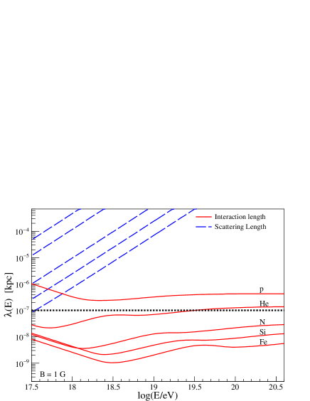
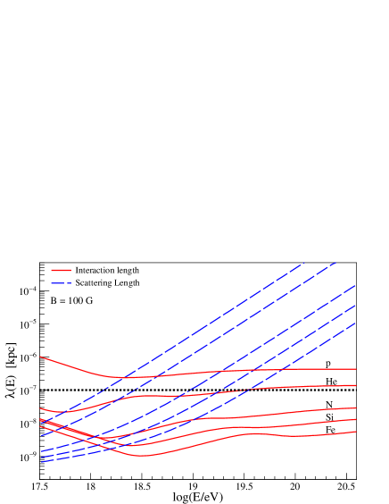
Figure 1: Interaction and scattering lengths of proton (p), helium (He), nitrogen (N), silicon (Si), and iron (Fe) as a function of energy. In both cases, the curves are ordered from bottom to top by decreasing primary mass. The dotted line corresponds to the radius of the sphere. (Top) $B=1$ G. (Bottom) $B=100$ G. The coherence length of the random magnetic field is $l_{c}=R/10$.

The bottom panel of the figure shows the interaction and the scattering lengths, but for $B=100$ G and $l_{c}=R/10$. As can be seen from the plot, the propagation in the random magnetic field of all nuclear species considered is diffusive at low energies and ballistic at high energies. Therefore, in general, the nuclei stay inside the sphere more time than in the case corresponding to $B=1$ G, and then the composition of the nuclei that leave the sphere becomes lighter compared with the one corresponding to that case.

It is assumed that the cosmic ray nuclei are accelerated in a region close to a supermassive black hole, in such a way that the energy spectrum is given by a power law with an exponential cutoff,

$$\varphi(E)=\varphi_{0}\,E^{-\Gamma}\exp\left(-\frac{E}{Z\,E_{max}^{p}}\right),$$ (5)

where $\varphi_{0}$ is a normalization constant, $\Gamma$ is the spectral index, $E_{max}^{p}$ is the maximum energy for the proton component, and $Z$ is the charge number of the nucleus. Note that the cutoff energy is proportional to the charge number, which is motivated by acceleration processes of electromagnetic origin Allard:05 ; AugerFit:17 . The spectral index is taken as $\Gamma=1$, which is motivated by acceleration mechanisms taking place in the accretion disks around massive black holes Blandford:76 and also by the fit of the flux and mass composition data obtained by Auger and reported in Ref. AugerFit:17 .

Figure 2 shows the energy spectra of the cosmic rays that leave the sphere corresponding to the injection of silicon (top panel) and nitrogen (bottom panel) nuclei at the center of the sphere. The injection spectrum of the nuclei is the one corresponding to Eq. (5) with $E_{max}^{p}=10^{18.5}$ eV. The magnetic field is such that $B=100$ G and $l_{c}=R/10$ (see bottom panel of Fig. 1).

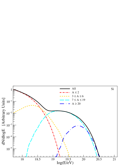
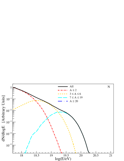
Figure 2: Energy spectra of nuclei that leave the sphere corresponding to silicon (top) and nitrogen (bottom). The magnetic field is such that $B=100$ G and $l_{c}=R/10$. The parameters of the injection spectrum are: $\Gamma=1$ and $E_{max}^{p}=10^{18.5}$ eV.

From the figure it can be seen that, for both nuclear species, a low energy light component is generated due to the interactions undergone by the primary nuclei during propagation through the sphere.

III Flux at Earth

The cosmic rays that leave the source environment are injected in the intergalactic medium and propagated from a given position in the Universe to Earth. The propagation of the particles is performed by using CRPropa 3. The simulations include photopion production and photodisintegration in the cosmic microwave background (CMB) and in the extragalactic background light (EBL), pair production on the CMB and on the EBL, nuclear decay, and the effects of the expansion of the Universe. The intergalactic magnetic field intensity is assumed to be negligible and then the propagation is unidimensional. A uniform distribution of sources in the Universe is assumed and the EBL model used in the simulations is the one developed in Ref. Kneiske:04 . The redshift range considered in the simulations starts at $z=0$ and ends at $z=5$.

The production of UHECRs over cosmological timescales is unknown. This source evolution is accounted by a function of the redshift $z$, $S(z)$. In this work, two cases are considered. $S(z)=1$, which corresponds to the case of no evolution of the sources and

$$S(z)=\left\{\begin{array}[]{ll}\left(1+z\right)^{5}&z\leq 1.7\\[5.69046pt] 2.7^{5}&1.7<z\leq 2.7\\[5.69046pt] 2.7^{5}\times 10^{2.7-z}&z>2.7\end{array}\right.,$$ (6)

which corresponds to the case of active galactic nuclei (AGN) of Ref. Aloisio:15 .

In order to fit the cosmic ray energy spectrum above $E=10^{17.5}$ eV, a galactic low energy iron component Unger:15 is assumed. The flux at Earth is supposed to be a power law with an exponential cutoff Aloisio:14 , which is given by

$$J_{G}(E)=c_{G}\ E^{-\Gamma_{G}}\exp\left(-\frac{E}{E_{cut}}\right),$$ (7)

where $\Gamma_{G}=3.29$ is the spectral index for energies below the ankle AugerICRC:17 , $E_{cut}$ is the cutoff energy of the galactic component, and $c_{G}$ is a normalization constant. The last two parameters are chosen in each model considered in order to fit the Auger spectrum.

Following Ref. AugerFit:17 , five nuclear species that are accelerated in the sources are considered: proton, helium, nitrogen, silicon, and iron.

The Auger energy spectrum reported in Ref. AugerICRC:17 is fitted by minimizing the $\chi^{2}$ given by

$$\chi^{2}=\sum_{i=1}^{N}\frac{\left(j_{i}-J_{G}(c_{G},E_{i})-\sum_{A}c_{A}J_{A}(E_{i})\right)^{2}}{\sigma_{i}^{2}},$$ (8)

where $j_{i}$ and $\sigma_{i}$ are the measured flux and its uncertainty, respectively, corresponding to the energy bin centered at energy $E_{i}$. Here $N$ is the number of energy bins considered in the fit and $A=\{\textrm{p, He, N, Si, Fe}\}$. The free fit parameters are $c_{G}$ and $c_{A}$, i.e., just the relative contributions of the different components are fitted. Note that the fitting parameters have to be positive or zero. This condition is fulfilled during the minimization procedure.

Figure 3 shows the fit of the Auger spectrum and the predicted mean value of the natural logarithm of the mass number $\langle\ln(A)\rangle$ and its variance $\textrm{Var}[\ln(A)]$ as a function of the primary energy compared with the experimental data obtained by Auger. The data points corresponding to the mean value of the natural logarithm of the mass number and its variance are obtained from the mean value and the variance of the $X_{max}$ parameter, which is reconstructed in an event-by-event basis from the data taken by the fluorescence telescopes of Auger AugerXmax:14 . Both quantities are obtained in Ref. AugerXmax:14 by using simulations of the showers with the high energy hadronic interaction model EPOS-LHC EPOSLHC:15 . It is worth mentioning that, $\langle\ln(A)\rangle$ as a function of primary energy, obtained by using EPOS-LHC, falls in between the ones corresponding to the two other models more frequently used in the literature, QGSJET-II-04 QGII:11 ; QGII:11b and Sibyll 2.3c Sibyll2.3c:15 . Moreover, $\langle\ln(A)\rangle$ obtained by using Sibyll 2.3c is above the one corresponding to EPOS-LHC, which in turn is above the one corresponding to QGSJET-II-04.

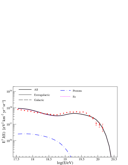
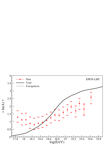
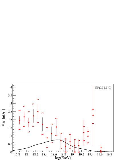
Figure 3: Fit of the UHECR spectrum (top) and the prediction for the mean value of the natural logarithm of the mass number (middle) and its variance (bottom). The experimental data were obtained by Auger AugerICRC:17 ; AugerXmax:14 and the high energy hadronic interaction model used in the composition analysis is EPOS-LHC. The parameters of the model are $L=10^{41}$ erg s^-1, $B=100$ G, $l_{c}=R/10$, $E_{max}^{p}=10^{18.5}$ eV, and $S(z)$ from Eq. (6).

The model of Fig. 3 assumes a luminosity of the photon gas $L=10^{41}$ erg s^-1, a random magnetic field of the source environment such that $B=100$ G and $l_{c}=R/10$, and the maximum energy of the injected proton component $E_{max}^{p}=10^{18.5}$ eV, i.e., the parameters used to obtain Fig. 2. The source evolution function considered is the one in Eq. (6). In the best fit scenario, the injected composition is dominated by iron nuclei with a small contribution of protons, as can be seen from the top panel of the figure, in which the contribution of the two components, obtained after propagation in the source environment and in the intergalactic medium, are shown. Note that, in this scenario, the galactic component appears at energies below $10^{17.5}$ eV. As can be seen from the figure, this model is not compatible with the Auger data. The reason for that is the very fast evolution of the sources at low redshift values, which increases the light component below the ankle, making the flux steeper than the one observed. Also the composition becomes progressively light for decreasing values of primary energy, which is inconsistent with the minimum in the $\langle\ln(A)\rangle$ observed at $10^{18.25}$ eV.

Considering the same scenario as before but for the case in which the sources do not evolve with redshift, i.e. $S(z)=1$, and for $B=1$ G, a good fit of the energy spectrum is obtained. In this case, the propagation in the source environment is not affected by the random magnetic field, as can be seen from the top panel of Fig. 1. The results corresponding to this model are shown in Fig. 4. In this case, the injection spectrum is dominated by helium, silicon, and iron; the proton and nitrogen contributions are negligible. In the top panel of the figure, the contributions of these three different nuclear species are shown, which are obtained after propagation in the source environment and in the intergalactic medium. In this case, the galactic component is not negligible in the energy range considered, as can be seen from the top panel of the figure (dashed line), and is such that $E_{cut}=10^{17.75}$ eV. Note that the discrepancies between the model predictions for $\textrm{Var}[\ln(A)]$ and the experimental data are larger at low energies, and this can be due to the too simple assumption for the composition of the galactic flux.

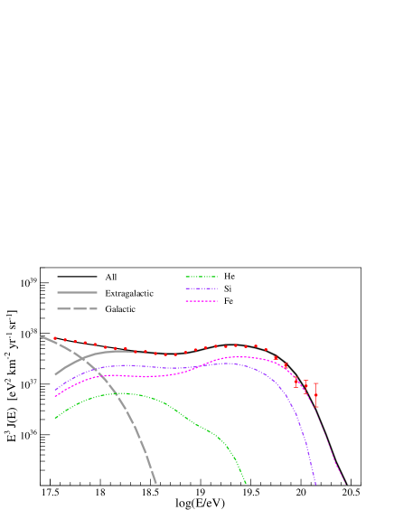
Figure 4: Same as Fig. 3, but for $B=1$ G and $S(z)=1$.

In order to study the influence of the random magnetic field present in the source environment, a scenario with the same parameters as the previous one (with $S(z)=1$) but for $B=100$ G is considered. As can be seen from Fig. 5, also in this case a good fit of the spectrum is obtained. In this scenario, the injected spectrum is dominated by silicon and iron nuclei, and as can be seen from the top panel of the figure, the contribution of the other components is negligible. From the middle panel of the figure, it can be seen that $\langle\ln(A)\rangle$ is smaller than the one corresponding to the previous scenario. This is due to the fact that increasing the magnetic field intensity increases the number of nuclei that propagate diffusively through the source environment (see Fig. 1). The particles that propagate in the diffusive regime travel larger path lengths, which causes an increase of the number of interactions, mainly photodisintegrations, undergone by them.

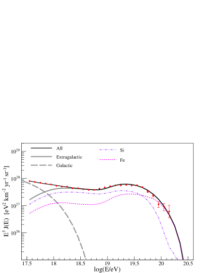
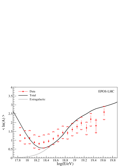
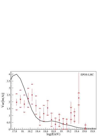
Figure 5: Same as Fig. 3, but for $S(z)=1$.

Photons and neutrinos are produced as a consequence of the UHECR propagation through the Universe. These secondary particles are generated by the decay of pions produced by the photopion production process undergone by the nuclei that interact with the low energy photons of the CMB and EBL. There is also a contribution to the neutrino component that comes from neutron decay. The only energy loss undergone by the neutrinos is the one corresponding to the adiabatic expansion of the Universe. Unlike what happens to the neutrinos, the high energy photons interact with the low energy photons of the CMB and EBL, initiating electromagnetic cascades that develop in the intergalactic medium. As a result, the photon flux at Earth spans from the ultrahigh energy region down to energies below 1 GeV. Therefore, the UHECRs can contribute to the low energy diffuse photon background.

The photon and neutrino fluxes corresponding to the two models compatible with the Auger data are calculated by using CRPropa 3. Figure 6 shows the $\gamma$-ray and neutrino fluxes for the model corresponding to Fig. 5 ($B=100$ G). As can be seen from the plot, the photon flux is smaller than the isotropic $\gamma$-ray background (IGRB) observed by the Fermi Large Aea Telescope (Fermi-LAT) FermiLATIGRB:15 . Moreover, the integral of the flux between 50 GeV and 2 TeV is $\sim 20$ times smaller than the 90% C.L. upper limit of Ref. Supanitsky:16 , which was obtained by using the Fermi-LAT analysis reported in Ref. FermiLATPRL:16 . Also, from the figure it can be seen that the secondary neutrino flux is much smaller than the upper limits obtained by IceCube IceCube:18 and by Auger AugerNu:17 . Similar results are obtained for the model of Fig. 4 ($B=1$ G). Low values of the $\gamma$-ray and neutrino fluxes are expected because it is very well known that the production of secondary particles, in models in which the high energy part of the cosmic ray flux is dominated by heavy nuclei, is much smaller than in the ones dominated by protons Aloisio:11 , which are still compatible with the neutrinos and $\gamma$-ray constraints in a region of the parametric space Supanitsky:16 ; Berezinsky:16 .

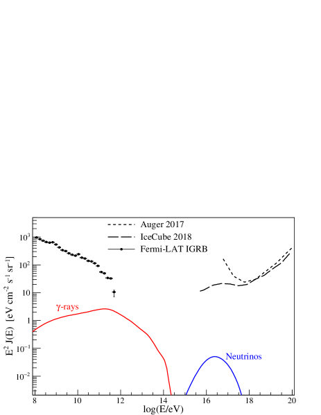
Figure 6: $\gamma$-ray and all flavors neutrino flux expected for the model of Fig. 5. The data points correspond to the IGRB obtained by Fermi-LAT FermiLATIGRB:15 . Also shown are the upper limits to the neutrino flux at 90% C.L., obtained by IceCube IceCube:18 and by Auger AugerNu:17 .

Increasing the luminosity of the photon gas present in the source environment makes the composition lighter; this is due to the decrease of the interaction lengths of the nuclei. In the limit of $\lambda_{PD},\,\lambda_{PP}\ll R$ all nuclear species are disintegrated before leaving the sphere, and then a light composition formed by protons and neutrons is obtained. It is found that models with $L\geq 5\times 10^{41}$ erg s^-1 are not compatible with the experimental data. Therefore, preferred models are such that $L\lesssim 10^{41}$ erg s^-1, which corresponds to low luminosity AGN (LLAGN) Ho:97 ; Ho:99 . It is worth noting that the central regions of these types of galaxies have been proposed as sources of the astrophysical neutrino flux observed by IceCube IceCubeNF:13 . In these models the high energy neutrinos are produced as a by-product of accelerated protons Kimura:15 ; Khiali:16 .

The redshift evolution of the sources is poorly known. In general, the source evolution of AGN is assumed to increase very fast between $z=0$ and $z=1-2$ (like in Eq. (6)) Hasinger:05 . However, in Ref. Kimura:15 a nonevolving luminosity function for LLAGN is assumed. This is the case of the scenarios developed in this work, which are compatible with the Auger data. The argument in Ref. Kimura:15 for this assumption is that LLAGN are similar to BL Lac objects (they both have a faint disk component), which have a luminosity function consistent with no evolution Ajello:14 .

It is worth mentioning that it is possible to fit the Auger spectrum assuming the evolution function of Ref. Kachel:17 , which corresponds to AGNs of $\log(L_{X}/\textrm{erg})=43.5$. However, the composition predicted in this case is heavier at high energies ($\gtrsim 10^{18.8}$ eV) and lighter at low energies ($\lesssim 10^{18.3}$ eV) than the one obtained by using EPOS-LHC to analyze the Auger data. The behavior of the high energy part of the composition profile is consistent with the results obtained in Ref. Kachel:17 . Therefore, also in this case the interaction of the nuclei with the protons present in a second region, surrounding the photon gas and filled with a proton gas, would be an appropriated mechanism to obtain a lighter composition at high energies, as it proposed in Ref. Kachel:17 .

In Ref. Kachel:17 , a one-dimensional approach for the propagation of the nuclei in the source environment is considered. In that approximation, only the diffusive regime of propagation is taken into account. The escape time used in these types of calculations is taken as $\tau(E)=\tau_{0}\,[E/(Z\,E_{0})]^{-\delta}$, where $\tau_{0}$ is a normalization constant, $E$ is the energy of the nucleus, $Z$ is its charge number, $E_{0}$ is a reference energy, and $\delta$ is a positive index. In the leaky box model approximation $\tau(E)\propto 1/D(E)$, where $D(E)$ is the diffusion coefficient. Therefore, the index $\delta$ gives the energy dependence of the diffusion coefficient. The escape time in these types of models is a decreasing function of the energy, which is valid up to a distance of the order of the size of the source environment region. Therefore, depending on the parameters used for the escape time in the one-dimensional calculation and the size of the source environment used in the three-dimensional approach, the high energy nuclei can escape from the source environment region before, compared to the case in which the particle propagates ballistically. In this case, a larger light component is expected at low energies for the three-dimensional calculation due to the larger number of photodisintegrations undergone by the high energy nuclei. This is the case for the model in which the source evolution function of Ref. Kachel:17 is considered. The larger number of light nuclei at low energies makes the composition lighter than the one obtained by Auger, using EPOS-LHC to interpret the data, and also a harder spectral index is required, $\Gamma=1$, to obtain a good fit of the spectrum compared to the one considered in Ref. Kachel:17 .

It should be noted that an independent composition analysis in the region of the spectrum below the ankle will be possible, in the near future, by using the information of the muon detectors of AMIGA (Auger Muons and Infill for the Ground Array) that are being installed at the Auger site Figueira:17 . As mentioned before, the muon content of the shower is very sensitive to the nature of the primary cosmic ray.

IV Conclusions

In this work, we have studied the possibility that the presumed extragalactic light component that dominates the UHECR flux below the ankle originates from the photodisintegration of more energetic and heavier nuclei in the photon gas present in the central regions of active galaxies. In this scenario, the UHECRs are accelerated near the supermassive black hole present in the central region of these galaxies. Note that these types of models require only one population of UHECR sources to explain the experimental data above $\sim 10^{18}$ eV.

We have found that low luminosity active galaxies with no source evolution are compatible with present composition and flux data, within the systematic uncertainties introduced by the high energy hadronic interaction models. It is worth mentioning that these types of astronomical objects have been proposed as the source of the high energy neutrinos observed by IceCube. We have also found that increasing the intensity of the random magnetic field in the source environment makes the composition observed at Earth lighter, as expected. However, we have proved that models with larger values of luminosity of the photon gas or with a strong source evolution are incompatible with present experimental data.

- (1) The Pierre Auger Collaboration, A. Aab et al., Nucl. Instrum. Meth. A 798, 172 (2015).
- (2) M. Fukushima et al., Prog. Theor. Phys. Suppl. 151, 206 (2003).
- (3) C. Patrignani et al., Chin. Phys. C 40 (2016) 100001.
- (4) F. Fenu for The Pierre Auger Collaboration, Proceedings of the 35th International Cosmic Ray Conference, Busan, Korea, PoS 486 (2017).
- (5) D. Ivanov for the Telescope Array Collaboration, Proceedings of the 35th International Cosmic Ray Conference, Busan, Korea, PoS 349 (2015).
- (6) D. Ivanov for the Pierre Auger Collaboration and the Telescope Array Collaboration, Proceedings of the 35th International Cosmic Ray Conference, Busan, Korea, PoS 498 (2017).
- (7) A. D. Supanitsky et al., Astropart. Phys. 29, 461 (2008).
- (8) T. Pierog, Proceedings of the 35th International Cosmic Ray Conference, Busan, Korea, PoS 1100 (2017).
- (9) The Pierre Auger collaboration, P. Aab et al., Phys. Rev. D 90, 122005 (2014).
- (10) The Telescope Array collaboration, R. Abbasi et al., Astropart. Phys. 64, 49 (2015).
- (11) V. de Souza for The Pierre Auger Collaboration, Proceedings of the 35th International Cosmic Ray Conference, Busan, Korea, PoS 522 (2017).
- (12) The Pierre Auger Collaboration, P. Abreu et al., Astrophys. J. Suppl. Ser. 203, 34 (2012).
- (13) R. Aloisio, V. Berezinsky, and P. Blasi, JCAP 10, 020 (2014).
- (14) M. Unger, G. Farrar, and L. Anchordoqui, Phys. Rev. D 92, 123001 (2015).
- (15) L. Anchordoqui, Proceedings of The European Physical Society Conference on High Energy Physics, Venice, Italy, PoS 001 (2017).
- (16) N. Globus, D. Allard, E. Parizot, and R. Mochkovitch, MNRAS 451, 751 (2015).
- (17) N. Globus, D. Allard, and E. Parizot, Phys. Rev. D 92, 021302 (2015).
- (18) M. Kachelrieß, O. Kalashev, S. Ostapchenko, and D. Semikoz, Phys. Rev. D 96, 083006 (2017).
- (19) R. Batista et al., JCAP 1605, 038 (2016).
- (20) A. Mücke, R. Engel, J. Rachen, R. Protheroe, and T. Stanev, Comp. Phys. Commun. 124, 290 (2000).
- (21) M. Kachelrieß, S. Ostapchenko, and R. Tomàs, New Journal of Physics 11, 065017 (2009).
- (22) A. Szabo and R. Protheroe, Astropart. Phys. 2, 375 (1994).
- (23) https://github.com/CRPropa/CRPropa3-data.
- (24) R. J. Protheroe, A. Meli and A. C. Donea, Space Sci. Rev. 107, 369 (2003).
- (25) D. Harari, S. Mollerach, and E. Roulet, Phys. Rev. D 89, 123001 (2014).
- (26) D. Allard, E. Parizot, A. Olinto, E. Khan, and S. Goriely, Astron. Astrophys. 443, L29 (2005).
- (27) The Pierre Auger collaboration, P. Aab et al., JCAP 04, 038 (2017).
- (28) R. Blandford, Mon. Not. Roy. Astron. Soc. 176, 465 (1976).
- (29) T. Kneiske, T. Bretz, K. Mannheim, and D. Hartmann, Astron. Astrophys. 413, 807 (2004).
- (30) R. Aloisio et al., JCAP 10, 006 (2015).
- (31) T. Pierog, I. Karpenko, J. Katzy, E. Yatsenko, and K. Werner Phys. Rev. C 92, 034906 (2015).
- (32) S. Ostapchenko, Phys. Rev. D 83, 014018 (2011).
- (33) S. Ostapchenko, Proceedings of the 32nd International Cosmic Ray Conference 2, 71 (2011).
- (34) F. Riehn, Proceedings of the 34th International Cosmic Ray Conference, The Hague, The Netherlands, PoS 558 (2015).
- (35) M. Ackermann et al., Astrophys. J.799, 86 (2015).
- (36) A. D. Supanitsky, Phys. Rev. D 94, 063002 (2016).
- (37) M. Ackermann et al., Phys. Rev. Lett. 116, 151105 (2016).
- (38) M. G. Aartsen et al., Phys. Rev. D 98, 062003 (2018).
- (39) E. Zas for The Pierre Auger Collaboration, Proceedings of the 35th International Cosmic Ray Conference, Busan, Korea, PoS 972 (2017).
- (40) R. Aloisio, V. Berezinsky, and A. Gazizov, Astropart. Phys. 34, 620 (2011).
- (41) V. Berezinsky, A. Gazizov, and O. Kalashev, Astropart. Phys. 84, 52 (2016).
- (42) L. Ho, A. Filippenko, and W. Sargent, The Astrophys. J. Suppl. Series 112, 315 (1997).
- (43) L. Ho, Astrophys. J. 516, 672 (1999).
- (44) M. Aartsen et al. (IceCube Collaboration), Science 342, 1242856 (2013).
- (45) S. Kimura, K. Murase, and K. Toma, Astrophys. J. 806, 159 (2015).
- (46) B. Khiali and E. Gouveia Dal Pino, MNRAS 455, 838 (2016).
- (47) G. Hasinger, T. Miyaji and M. Schmidt, Astron. Astrophys. 441, 417 (2005).
- (48) M. Ajello et al., Astrophys. J. 780, 73 (2014).
- (49) J.M. Figueira for the Pierre Auger Collaboration, Proceedings of the 35th International Cosmic Ray Conference, Busan, Korea, PoS 396 (2017).