Homogenization of edge-dislocations as a weak limit of de-Rham currents

Abstract

In the material science literature we find two continuum models for crystalline defects: (i) A body with (finite) isolated defects is typically modeled as a Riemannian manifold with singularities, and (ii) a body with continuously distributed defects, which is modeled as a smooth (non-singular) Riemannian manifold with an additional structure of an affine connection. In this work we show how continuously distributed defects may be obtained as a limit of singular ones . The defect structure is represented by layering $1$-forms and their singular counterparts - de-Rham $(n-1)$ currents. We then show that every smooth layering $1$-form may be obtained as a limit, in the sense of currents, of singular layering forms, corresponding to arrays of edge dislocations. As a corollary, we investigated manifolds with full material structure, i.e., a complete co-frame for the co-tangent bundle. We define the notion of singular torsion current for manifolds with a parallel structure and prove its convergence to the regular smooth torsion tensor at homogenization limit. Thus establishing the so-called emergence of torsion at the homogenization limit.

1 Introduction

The study of material defects, and notably dislocations, is a central theme in material science. The modeling of solid bodies, with or without defects, often follows a paradigm in which the elemental object is that of a body manifold: solid bodies are modeled as geometric objects—manifolds—and their internal structure is represented by additional structure such as a frame field, a metric or an affine connection. The mechanical properties of the body enter through a constitutive relation, whose structure is correlated with the geometric structure of the body.

There have been two distinct approaches to the modeling of body manifolds with dislocations:

1. Isolated dislocations: One starts with a defect-free body, which is either modeled as a compact subset of Euclidean space, or as a perfect lattice. Defects are introduced by Volterra cut-and-weld protocols Vol07 ; see Figure 1. Note that a perfect lattice may be related to a Euclidean structure by assigning lengths and angles to inter-particle bonds.

   

   

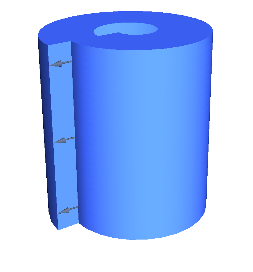
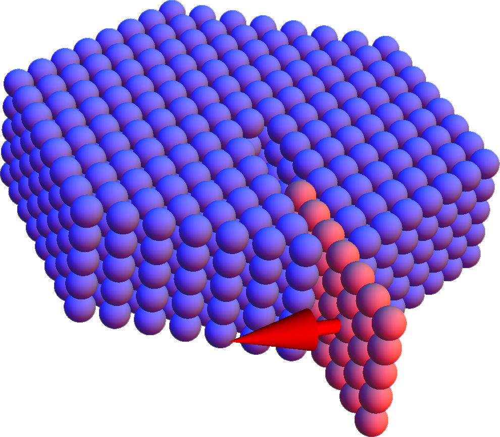
   Figure 1: Left: An edge-dislocation generated by a cut-and-weld protocol in a continuum setting. Right: An edge-dislocation generated by removing a half-plane in a lattice.

2. Distributed dislocations: In the classical literature from the 1950s, the body is modeled as a smooth manifold endowed with a curvature-free affine connection Nye53 ; Kon55 ; BBS55 ; Kro81 . If, in addition, one adds a basis of the tangent space at one point, then the affine connection induces a smooth frame field, which is the kinematic model, for example, in Dav86 . In later literature YG12 , the continuum model is that of a Weitzenböck manifold, which is a smooth manifold endowed with a Riemannian metric and a metrically-consistent, curvature-free affine connection (in fact, the vanishing curvature condition has to be replaced by the even stronger condition of trivial holonomy). Note that a frame field induces an intrinsic metric, so that all three descriptions are essentially identical. The density of the dislocations is identified with the torsion tensor of the affine connection.

A longstanding problem has been to rigorously justify the continuum model of distributed dislocations as a limit of (properly scaled) isolated dislocations, as their number tends to infinity, in the spirit of other homogenization theories. Such an analysis was recently presented in KM15 ; KM16 . Specifically, bodies with either isolated or distributed dislocations were modeled as Weitzenböck manifolds $({\mathcal{M}},\mathfrak{g},\nabla)$. In the case of isolated dislocations, the smooth part of the manifold is multiply-connected, the defects being located inside either non-smooth sets, or “holes”, and the connection is the Riemannian (Levi-Civita) connection. A sequence of multiply-connected body manifolds with isolated dislocations may converge to a simply-connected body manifold $({\mathcal{M}},\mathfrak{g},\nabla)$, where $\nabla$ is non-symmetric; that it, torsion arises as a weak limit of torsion-free connections. Moreover, it was shown that every triple $({\mathcal{M}},\mathfrak{g},\nabla)$ can be obtained as a limit of bodies with isolated dislocations.

The work KM15 ; KM16 has several shortcomings: (i) The notion of convergence was tailored to the problem, and as a result, does not coincide with prevalent notions of convergence. (ii) The standard mathematical apparatus accounting for singularities is generalized functions (or generalized sections), thus providing a natural setting for convergence. This has been missing here. (iii) In particular, one would hope to recover a notion of singular torsion, in the same spirit as one obtains a notion of singular curvature for cone singularities. (iv) This analysis requires the consideration of a complete lattice structure, not including, for example, scalar elastic invariants.

An alternative approach to defects, and notably to dislocations, was proposed by Epstein and Segev ES14 . Their point of view is that every material structure is represented by one or more differential forms: while smooth structures are represented by smooth differential forms, singularities in structure are represented by their distributional counterparts—de-Rham currents.

Specifically, ES14 models the structure of a lattice by means of differential forms termed layering forms which represent Bravais surfaces. In $n$ dimensions, the prescription of a set of $n$ linearly-independent 1-forms $\vartheta^{i}$ (a coframe) amounts to Davini’s frame field approach Dav86 , but the points in ES14 are:

1. A single layering form may suffice to track the presence of defects.

2. Layering forms can be singular.

In the absence of defects, the layering forms are closed, namely,

$$d\vartheta^{i}=0.$$

In the case of distributed defects, we expect $d\vartheta^{i}\neq 0$, where the 2-form $d\vartheta^{i}$ is related to the density of the defects.

The prescription of $n$ linearly-independent layering forms defines an intrinsic metric, $\sum_{i}\vartheta^{i}\otimes\vartheta^{i}$ and a material connection, whose path-independent parallel transport $\Pi_{p}^{q}:T_{p}{\mathcal{M}}\to T_{q}{\mathcal{M}}$ between two points $p,q\in{\mathcal{M}}$ is given by

$$\Pi_{p}^{q}={e_{i}}|_{q}\otimes{\vartheta^{i}}|_{p},$$

where $\{e_{i}\}$ is the frame field dual to $\{\vartheta^{i}\}$ (here and below we adopt Einstein’s summation convention). The generalization of this approach to structures with singularities is as follows: to every smooth 1-form $\vartheta^{i}$ corresponds an $(n-1)$-current

$$T_{\vartheta^{i}}(\alpha)=\int_{\mathcal{M}}\vartheta^{i}\wedge\alpha,\qquad\alpha\in\Omega^{n-1}_{c}({\mathcal{M}}),$$

where $\Omega^{k}_{c}({\mathcal{M}})$ denotes the module of smooth, compactly-supported $k$-forms on ${\mathcal{M}}$ (see Section 2 for a short review of de-Rham currents). By definition, the boundary of an $(n-1)$-current is an $(n-2)$-current

$$\partial T_{\vartheta^{i}}(\beta)=\int_{\mathcal{M}}\vartheta^{i}\wedge d\beta=\int_{\mathcal{M}}d\vartheta^{i}\wedge\beta\qquad\beta\in\Omega^{n-2}_{c}({\mathcal{M}}),$$

where the second identity follows from integration by parts and the compact support of $\beta$. If $\vartheta^{i}$ is closed then $\partial T_{\vartheta^{i}}=0$, i.e., the absence of defects is reflected by the vanishing of the boundary of the current induced by $\vartheta^{i}$. Just like in classical distribution theory, not every $(n-1)$-current is induced by a smooth 1-form; structures with singularities are modeled by $(n-1)$-currents; the defects are associated with the boundary of those currents that are not induced by smooth forms.

In this work, we show that the homogenization of singular defects can be cast in the framework of weak convergence of currents. To set the stage, we review in Section 2 some basic facts about de-Rham currents. In Section 3, we consider an arbitrary (generally non-closed) smooth layering form $\beta\in\Omega^{1}({\mathcal{M}})$ on the two-dimensional square ${\mathcal{M}}=[0,1]^{2}$, which we view as representing distributed edge-dislocations. We develop a generic construction of a layering form $\nu$, which approximate $\beta$ (in a sense made precise), while being smooth and closed everywhere, except on a one-dimensional sub-manifold $\Gamma$. Furthermore, interpreting the layering form $\nu$ as a 1-current, we show that the boundary of that current is supported on $\Gamma$. Thus, view the layering form $\nu$ as representing a singular edge-dislocation, whose locus is $\Gamma$, and whose intensity is equal to the total intensity of the layering form $\beta$.

In Section 4,we show that every (possibly non-closed) $1$-form $\beta\in\Omega^{1}({\mathcal{M}})$ can be approximated by a sequence of discontinuous layering forms $\nu^{(n)}$, representing an $n$-by-$n$ array of edge-dislocations. We construct $\nu^{(n)}$ by gluing together properly rescaled versions of the form constructed in Section 3. We then prove that $T_{\nu^{(n)}}$ converges as $n\to\infty$ to a 1-current $T_{\beta}$; the convergence is in the sense of weak convergence of currents. We interpret this limit theorem as a statement that every smooth distribution if dislocations is a limit, in the sense of weak convergence of currents, of singular dislocations.

In Section 5, we generalize the analysis to the case where ${\mathcal{M}}$ is an $n$ dimensional manifold equipped with a full lattice structure, that is, a (possibly singular) frame field $\{e_{i}\}_{i=1}^{n}$. We cast in the setting of currents the convergence of parallel transport and torsion. In particular, we define the notion of singular torsion, and show that “the emergence of torsion” as a limit of torsion-free connections, as exposed in KM15 , should be re-interpreted as a convergence of singular torsions to a limiting smooth torsion. Further extensions and concluding remarks are presented in Section LABEL:sec:discussion.

2 De-Rham currents

We start by reviewing the definition of de-Rham currents on manifolds, which are fundamental objects representing singular material structures. For a full introduction see for example the classical monograph of Federer Fed69 or de-Rhams deR84 . For more recent reviews see also LY02 ; KP08 .

Let ${\mathcal{M}}$ be a smooth, compact, orientable $n$-dimensional manifold with boundary. For every $1\leq k\leq n$, let $\Omega^{k}({\mathcal{M}})$ denote the space of smooth $k$-forms on ${\mathcal{M}}$ and let

$$\Omega_{c}^{k}({\mathcal{M}})=\left\{\omega\in\Omega^{k}({\mathcal{M}})~{}:~{}\operatorname{supp}(\omega)\Subset{\mathcal{M}}\right\}$$

be the module of smooth $k$-forms compactly-supported in ${\mathcal{M}}$. Choose a Riemannian metric $g$ on ${\mathcal{M}}$, and define for every compact $K\Subset{\mathcal{M}}$ a family of seminorms $\phi_{K,j}^{k}:\Omega_{c}^{k}({\mathcal{M}})\to{\mathbb{R}}^{+}$ by

$$\phi_{K,j}^{k}(\omega)=\sup_{0\leq i\leq j}\|D^{i}\omega\|_{K},$$

where $D^{i}\omega:{\mathcal{M}}\to{\operatorname{Hom}}(\otimes^{i}T{\mathcal{M}},\Lambda^{k}T^{*}{\mathcal{M}})$ is the $i$-th differential of $\omega$ (not to be confused with the exterior derivative), and

$$\|D^{i}\omega\|_{K}=\sup_{p\in K}\|(D^{i}\omega)_{p}\|,$$

where $\|\cdot\|$ is the norm on ${\operatorname{Hom}}(\otimes^{i}T{\mathcal{M}},\Lambda^{k}T^{*}{\mathcal{M}})$ induced by the metric $g$. Since ${\mathcal{M}}$ is compact, a different choice of $g$ will give equivalent seminorms; as a result, it makes sense to say that a $k$-form is $C^{j}$-bounded without reference to any metric. The seminorms $\phi_{K,j}^{k}$ turn

$$\Omega_{K}^{k}({\mathcal{M}})=\{\omega\in\Omega_{c}^{k}({\mathcal{M}})~{}:~{}\operatorname{supp}(\omega)\subset K\}$$

into a Fréchet space, that is, a locally-convex topological vector space which is complete with respect to a translationally-invariant metric (Rud91, , p. 9).

Endow $\Omega_{c}^{k}({\mathcal{M}})$ with the finest topology for which the inclusion maps

$$\Omega_{K}^{k}({\mathcal{M}})\hookrightarrow\Omega_{c}^{k}({\mathcal{M}})$$

are continuous for all compact $K\Subset{\mathcal{M}}$. It follows that a sequence $\omega_{n}\in\Omega_{c}^{k}({\mathcal{M}})$ converges in this topology to $0$ if and only if there exists a compact set $K\Subset{\mathcal{M}}$ such that $\operatorname{supp}(\omega_{n})\subset K$ for all $n$, and $\omega_{n}\to 0$ in the topology of $\Omega_{K}^{k}({\mathcal{M}})$ described above.

Finally, let $\mathscr{D}_{k}({\mathcal{M}})$ be the dual vector space of continuous linear functionals on $\Omega_{c}^{k}({\mathcal{M}})$; the members of $\mathscr{D}_{k}({\mathcal{M}})$ are called de-Rham $k$-currents. Equivalently, a linear functional $T:\Omega_{c}^{k}({\mathcal{M}})\to{\mathbb{R}}$ is a $k$-current if and only if there exists for every $K\Subset{\mathcal{M}}$ an $N=N(K)\in\mathbb{N}$ and a constant $C=C(K)>0$, such that for every $\omega\in\Omega_{K}^{k}({\mathcal{M}})$,

$$|T(\omega)|\leq C\,\sup_{1\leq j\leq N}\phi_{K,j}^{k}(\omega).$$

We endow $\mathscr{D}_{k}({\mathcal{M}})$ with the weak-star topology: a sequence of $k$-currents $T_{n}$ converges to a $k$-current $T$ if

$$\lim_{n\to\infty}T_{n}(\omega)=T(\omega)$$

for every $\omega\in\Omega_{c}^{k}({\mathcal{M}})$. The support of a $k$-current $T\in\mathscr{D}_{k}({\mathcal{M}})$ is defined by $\operatorname{supp}(T)={\mathcal{M}}\setminus A(T)$, where $A(T)$ is the annihilation set of $T$, i.e., the union of all open subsets $U\subset{\mathcal{M}}$ for which $T(\alpha)=0$ whenever $\operatorname{supp}(\alpha)\subset U$.

For example, every locally-integrable $k$-form $\beta$ defines an $(n-k)$-current $T_{\beta}\in\mathscr{D}_{n-k}({\mathcal{M}})$ by

$$T_{\beta}(\alpha)=\int_{\mathcal{M}}\beta\wedge\alpha.$$

In other words, currents may be viewed as generalized differential forms. Currents also generalize the concept of a submanifold. Let $S\subset{\mathcal{M}}$ be a $k$-dimensional oriented submanifold, then $S$ induces a $k$-current $[S]$ given by

$$[S](\alpha)=\int_{S}\alpha,\quad\alpha\in\Omega_{c}^{k}({\mathcal{M}}).$$

The boundary operator of a $k$-current is a map $\partial:\mathscr{D}_{k}({\mathcal{M}})\to\mathscr{D}_{k-1}({\mathcal{M}})$, defined by

$$\partial T(\alpha)=T(d\alpha),\quad\alpha\in\Omega_{c}^{k-1}({\mathcal{M}}).$$

Since $d^{2}=0$, it immediately follows that $\partial^{2}=0$; moreover, it follows from integration by parts and Stokes theorem that

$$\partial T_{\beta}=(-1)^{k-1}T_{d\beta}$$

for every smooth $k$-form $\beta$,

3 Layering form for an edge-dislocation

As discussed in Epstein (Eps10, , Section 4.5.3) and SE14, a single differential 1-form is capable of capturing the presence of a dislocation. A covector $\omega$ in a vector space $V$ induces a family of hyperplanes (Bravais planes),

$$H_{t}=\{v\in V~{}:~{}\omega(v)=t\}$$

foliating $V$; the action of $\omega$ on a vector $v\in V$ can be viewed as “the number of hyperplanes” intersected by the vector $v$. In the case of a smooth manifold ${\mathcal{M}}$, given a 1-form $\nu$ and an oriented curve $C\subset{\mathcal{M}}$, the integral

$$\int_{C}\nu$$

can be interpreted as the (signed) number of $\nu$-hyperplanes intersected by $C$. Thus, a single 1-form $\nu$ on a manifold ${\mathcal{M}}$, can be viewed as representing a layering form—a density of a family of parallel layers at each point.

A 1-form $\nu$ induces a smooth layering structure (foliation) for ${\mathcal{M}}$ if it is integrable; that is, if ${\mathcal{M}}$ can be foliated such that the tangent bundle of each leaf coincides with the kernel of $\nu$. It is well known that a sufficient and necessary condition for $\nu$ to induce a smooth layering structure is that

$$d\nu=\alpha\wedge\nu$$

for some $(n-1)$-form $\alpha$ (Lee12, , Chap. 19). Note that for a simply-connected two-dimensional manifold, every non-vanishing 1-form induces a smooth layering structure.

If, in addition, the 1-form $\nu$ is closed, $d\nu=0$, then it follows from Stokes’ theorem that for every simple, oriented, closed curve $C\subset{\mathcal{M}}$, the sum of all the hyperplanes intersected by $C$ vanishes,

$$\int_{C}\nu=\int_{\Sigma_{C}}d\nu=0,$$ (1)

where $\Sigma_{C}\subset{\mathcal{M}}$ is any $2$ dimensional submanifold of ${\mathcal{M}}$ bounded by $C$. In other words, there are no “extra” layers, and the layering structure is defect-free. Motivated by equation (1), we may interpret $d\nu$ as a defect density.

Suppose in turn that $\nu$ is a 1-form corresponding to an isolated dislocation concentrated on a hyper-surface $\Gamma\subset{\mathcal{M}}$. By (1), $d\nu=0$ on ${\mathcal{M}}\setminus\Gamma$, and consequently, $\nu$ must be singular at $\Gamma$.

We next construct an explicit layering form on a two-dimensional manifold, which may represent a singular edge-dislocation in one family of Bravais planes. We first consider a topological rectangle, i.e., a manifold that can be parametrized as follows:

$${\mathcal{M}}=[0,1]^{2}=\{(x,y)~{}:~{}0\leq x,y\leq 1\}.$$

We denote the left, right, top and bottom edges of ${\mathcal{M}}$ by ${\mathcal{M}}_{\text{left}},$ ${\mathcal{M}}_{\text{right}}$, ${\mathcal{M}}_{\text{top}}$ and ${\mathcal{M}}_{\text{bottom}}$, respectively. The locus of the dislocation is a one-dimensional submanifold, with we take to be the closed parametric segment

$$\Gamma_{a}=[1/2-a/2,1/2+a/2]\times\{1/2\}\subset{\mathcal{M}},$$ (2)

where $0<a<1$ is a parameter, which will be used later in our homogenization procedure.

Proposition 1

Let $\beta\in\Omega^{1}({\mathcal{M}})$ be a nowhere-vanishing 1-form and let $0<a<1$. Then, there exists a continuously differentiable 1-form $\nu_{a}$ on ${\mathcal{M}}\setminus\Gamma_{a}$ satisfying the following properties:

1. $\nu_{a}$ is $C^{1}$-bounded (see definition in Section 2).

2. $\nu_{a}$ is closed.

3. $\nu_{a}$ coincides with $\beta$ on ${\mathcal{M}}_{\text{left}}$ and ${\mathcal{M}}_{\text{right}}$.

4. $\nu_{a}$ has the same circulation as $\beta$,

   $$\int_{\partial{\mathcal{M}}}\nu_{a}=\int_{\partial{\mathcal{M}}}\beta.$$

5. The horizontal components of $\nu_{a}$ and $\beta$ coincide,

   $$\nu_{a}(\partial_{x})=\beta(\partial_{x}),$$

   whenever $|x-1/2|>a/2$.

Before proving Proposition 1, we show in which sense the 1-form $\nu_{a}$ represents a family of Bravais planes dislocated along the segment $\Gamma_{a}$. Since $\nu_{a}$ is closed in ${\mathcal{M}}\setminus\Gamma_{a}$, it follows that

$$\oint_{C}\nu_{a}=0$$

along every contractible loop $C$ in ${\mathcal{M}}\setminus\Gamma_{a}$.

Let $\mathfrak{g}$ be a metric on ${\mathcal{M}}$, and denote by $\Gamma_{a}^{\varepsilon}$, $\varepsilon>0$, a family of $\varepsilon$-tubular neighborhoods of $\Gamma_{a}$. By Stokes’ law, for every small enough $\varepsilon>0$,

$$\begin{split}0&=\int_{{\mathcal{M}}\setminus\Gamma_{a}^{\varepsilon}}d\nu_{a}=\int_{\partial{\mathcal{M}}}\nu_{a}-\int_{\partial\Gamma_{a}^{\varepsilon}}\nu_{a}.\end{split}$$

Since $\nu_{a}$ has the same circulation as $\beta$,

$$\int_{\partial\Gamma_{a}^{\varepsilon}}\nu_{a}=\int_{\partial{\mathcal{M}}}\beta.$$

Letting $\varepsilon\to 0$, we obtain

$$\int_{\Gamma_{a}}[\nu_{a}]=\int_{\partial{\mathcal{M}}}\beta,$$ (3)

where $[\nu_{a}]$ is the discontinuity jump of $\nu_{a}$ along $\Gamma_{a}$, whose sign is determined by the orientation of ${\mathcal{M}}$ (hence of $\Gamma_{a}^{\varepsilon}$) and $\Gamma_{a}$. Note that the $1$-sided limits of $\nu_{a}$ at $\Gamma_{a}$ exist since $\nu_{a}$ is $C^{1}$-bounded. Moreover, since ${\mathcal{M}}$ is compact, the identity (3) does not depend on the choice of the metric $\mathfrak{g}$.

Thus, the defining properties of $\nu_{a}$ imply that it does not satisfy the integral version (1) of closedness, and as a result, must have a singularity along $\Gamma_{a}$.

Remark 1

The singular set $\Gamma_{a}$ of $\nu_{a}$ is evidently uncountable. Generally, if ${\mathcal{M}}$ is a compact two-dimensional manifold with or without boundary, $\Gamma$ is a submanifold of ${\mathcal{M}}$, and $\nu$ is a $C^{0}$-bounded closed 1-form on ${\mathcal{M}}\setminus\Gamma$, such that there exists a closed curve $C$ for which

$$\oint_{C}\nu\neq 0,$$

then $\Gamma$ cannot be a finite set. Suppose, by contradiction that $\Gamma=\{p_{1},p_{2},\ldots,p_{k}\}$ is finite, and assume without loss of generality that all the points in $\Gamma$ are enclosed by the curve $C$. Assuming as above a metric $\mathfrak{g}$, setting $\Gamma^{\varepsilon}=\cup_{i}B_{\varepsilon}(p_{i})$, and performing the same calculation,

$$\sum_{i=1}^{k}\oint_{\partial B_{\varepsilon}(p_{i})}\nu=-\oint_{C}\nu.$$

If $\nu$ is bounded, then the left-hand side vanishes as $\varepsilon\to 0$, yielding a contradiction. The physical interpretation of this observation is that there is no such thing as an edge-dislocation supported at a point (or on a line in three dimensions).

of Proposition 1.

∎We construct $\nu_{a}$ as the differential of a discontinuous function $f$. First, define $f_{0}:\partial{\mathcal{M}}\to{\mathbb{R}}$ by fixing $q_{0}=(1,1/2)$ and letting

$$f_{0}(q)=\int_{q_{0}}^{q}\beta,$$

where the integration from $q_{0}$ to $q$ is along $\partial{\mathcal{M}}$ counterclockwise. If the circulation of $\beta$ is non-zero, then $f_{0}$ is discontinuous at $q_{0}$. However, its differential is well-defined and smooth at $q_{0}$ as it coincides with the tangential component of $\beta$.

Next, let

$${\mathcal{M}}_{a}=[1/2-a/2,1/2+a/2]\times[0,1],$$

and define $\bar{f}:{\mathcal{M}}\setminus{\mathcal{M}}_{a}\to{\mathbb{R}}$ by integrating $\beta$ horizontally, from the boundaries inward,

$$\bar{f}(x,y)=\begin{cases}f_{0}(0,y)+\int_{[(0,y),(x,y)]}\beta,\quad&x<1/2-a/2\\ f_{0}(1,y)+\int_{[(1,y),(x,y)]}\beta,\quad&x>1/2+a/2.\end{cases}$$

Denote by $p_{L},p_{R}:{\mathcal{M}}\to{\mathbb{R}}$ the second-order Taylor expansions of $\bar{f}$ about $x_{L}=1/2-a/2$ and $x_{R}=1/2+a/2$ along the $x$-direction, i.e.,

$$p_{L}(x,y)=\bar{f}(x_{L},y)+\frac{\partial\bar{f}}{\partial x}(x_{L},y)(x-x_{L})+\frac{1}{2}\frac{\partial^{2}\bar{f}}{\partial x^{2}}(x_{L},y)(x-x_{L})^{2}$$

$$p_{R}(x,y)=\bar{f}(x_{R},y)+\frac{\partial\bar{f}}{\partial x}(x_{R},y)(x-x_{R})+\frac{1}{2}\frac{\partial^{2}\bar{f}}{\partial x^{2}}(x_{R},y)(x-x_{R})^{2}.$$

Let $r\in C^{\infty}({\mathbb{R}})$ be a monotonically-increasing function satisfying,

$$r(t)=0\quad\forall t\leq-1/2\qquad\text{ and }\qquad r(t)=1\quad\forall t\geq 1/2.$$

We extend $\bar{f}$ to ${\mathcal{M}}\setminus\Gamma_{a}$ by interpolating between $p_{L}$ and $p_{R}$, using the smooth “connecting” function $r$ (see Figure 2),

$$f(x,y)=\begin{cases}\bar{f}(x,y)&|x-1/2|\geq a/2\\ (1-r(\frac{x-1/2}{a}))p_{L}(x,y)+r(\frac{x-1/2}{a})p_{R}(x,y)&|x-1/2|<a/2.\end{cases}$$ (4)

Figure 2: The three stages in the construction of $f$: first $f_{0}$ is defined on $\partial{\mathcal{M}}$; next $\bar{f}$ is defined on the set $|x-1/2|>a/2$ by integrating the horizontal component of $\beta$ from the nearest vertical boundary; finally, $f$ is extended to the set $|x-1/2|\leq a/2$ by interpolation. The dashed segment connecting $\Gamma_{a}$ to $q_{0}$ is the discontinuity line of $f$.

We turn to evaluate $\nu_{a}=df$ by differentiating (4). For $x>a/2+1/2$,

$$\begin{split}df_{(x,y)}&=\left(\frac{\partial}{\partial x}\left(\int_{[(1,y),(x,y)]}\beta\right)\right)dx+\left(\frac{\partial f_{0}}{\partial y}(1,y)+\frac{\partial}{\partial y}\left(\int_{[(1,y),(x,y)]}\beta\right)\right)dy\\ &=\beta_{1}(x,y)\,dx+\left(\beta_{2}(1,y)+\int_{1}^{x}\frac{\partial\beta_{1}}{\partial y}(x^{\prime},y)dx^{\prime}\right)dy,\end{split}$$ (5)

where $\beta_{1}$ and $\beta_{2}$ are the components of $\beta$,

$$\beta=\beta_{1}\,dx+\beta_{2}\,dy.$$

Similarly, for $x<1/2-a/2$,

$$df_{(x,y)}=\beta_{1}(x,y)\,dx+\left(\beta_{2}(0,y)+\int_{0}^{x}\frac{\partial\beta_{1}}{\partial y}(x^{\prime},y)dx^{\prime}\right)dy.$$ (6)

While $f$ has a discontinuity along the segment $[1/2+a,1]\times\{1/2\}$, its one-sided derivatives along this segment are continuous, as they are expressed in terms of the smooth 1-form $\beta$. Moreover,

$$df|_{{\mathcal{M}}_{\text{left}}}=\beta|_{{\mathcal{M}}_{\text{left}}}\qquad\text{ and }\qquad df|_{{\mathcal{M}}_{\text{right}}}=\beta|_{{\mathcal{M}}_{\text{right}}},$$

proving Property (iii). Likewise, for $|x-1/2|\geq a/2$,

$$df(\partial_{x})=\beta_{1}=\beta(\partial_{x}),$$

proving Property (v).

For $(x,y)\in{\mathcal{M}}_{a}$,

$$\begin{split}df_{(x,y)}&=\frac{1}{a}r^{\prime}\left(\tfrac{x-1/2}{a}\right)(p_{R}(x,y)-p_{L}(x,y))dx\\ &+\left[\left(1-r\left(\tfrac{x-1/2}{a}\right)\right)\frac{\partial p_{L}}{\partial x}(x,y)+r\left(\tfrac{x-1/2}{a}\right)\frac{\partial p_{R}}{\partial x}(x,y)\right]dx\\ &+\left[\left(1-r\left(\tfrac{x-1/2}{a}\right)\right)\frac{\partial p_{L}}{\partial y}(x,y)+r\left(\tfrac{x-1/2}{a}\right)\frac{\partial p_{R}}{\partial y}(x,y)\right]dy.\end{split}$$ (7)

The 1-form $df$ is continuous at $x=1/2\pm a/2$, for example,

$$\begin{split}\lim_{x\nearrow 1/2+a/2}df(x,y)&=\frac{\partial p_{R}}{\partial x}(1/2+a/2,y)\,dx+\frac{\partial p_{R}}{\partial y}(1/2+a/2,y)\,dy\\ &=\frac{\partial\bar{f}}{\partial x}(1/2+a/2,y)\,dx+\frac{\partial\bar{f}}{\partial y}(1/2+a/2,y)\,dy\\ &=d\bar{f}(1/2+a/2,y).\end{split}$$

A second differentiation shows that $\nu_{a}$ is continuously-differentiable at $x=1/2\pm a/2$. This together with (7) proves Property (i) and consequently also Property (ii).

It remains to prove Property (iv), that $df$ and $\beta$ have the same circulations. This follows from our construction of $f_{0}$ on $\partial{\mathcal{M}}$,

$$\begin{split}\int_{\partial{\mathcal{M}}}df&=\lim_{\varepsilon\to 0}\left(f(1,1/2-\varepsilon)-f(1,1/2+\varepsilon)\right)\\ &=\lim_{\varepsilon\to 0}\left(f_{0}(1,1/2-\varepsilon)-f_{0}(1,1/2+\varepsilon)\right)\\ &=\int_{\partial{\mathcal{M}}}\beta.\end{split}$$

∎∎

The 1-form $\nu_{a}$ (which is only defined on ${\mathcal{M}}\setminus\Gamma_{a}$) induces a 1-current on ${\mathcal{M}}$,

$$T_{\nu_{a}}(\alpha)=\int_{\mathcal{M}}\nu_{a}\wedge\alpha\qquad\alpha\in\Omega_{c}^{1}({\mathcal{M}}).$$

Its boundary is the 0-current,

$$\partial T_{\nu_{a}}(f)=T_{\nu_{a}}(df)=\int_{\mathcal{M}}\nu_{a}\wedge df\qquad f\in C_{c}^{\infty}({\mathcal{M}}).$$

Integrating by parts, we obtain

$$\partial T_{\nu_{a}}(f)=\int_{\Gamma_{a}}f[\nu_{a}],$$

where for $|x-1/2|<a/2$,

$$\begin{split}[\nu_{a}](x)&=\lim_{\varepsilon\to 0}\left(df(x,1/2+\varepsilon)-df(x,1/2-\varepsilon)\right)\\ &=\frac{1}{a}r^{\prime}\left(\tfrac{x-1/2}{a}\right)\,\lim_{\varepsilon\to 0}\left(p_{R}(x,1/2+\varepsilon)-p_{R}(x,1/2-\varepsilon)\right)\\ &=\frac{1}{a}r^{\prime}\left(\frac{x-1/2}{a}\right)\,\int_{\partial{\mathcal{M}}}\beta.\end{split}$$

To conclude, we view $\nu_{a}$ as a layering form on ${\mathcal{M}}$ having an edge-dislocation concentrated on the hyper-surface $\Gamma_{a}$. The locus of the dislocation is revealed by the boundary of the differential current induced by $\nu_{a}$. Note that ${\mathcal{M}}\setminus\Gamma_{a}$ is defect-free only to the extent detectable by $\nu_{a}$. Generally, ${\mathcal{M}}\setminus\Gamma_{a}$ may contain defects detected by other layering forms.

4 Homogenization of distributed edge-dislocations

We proceed to construct a singular layering form corresponding to an $n$-by-$n$ array of edge-dislocations, each of magnitude of order $1/n^{2}$, using Proposition 1 as a building block.

For $(x_{0},y_{0})\in{\mathbb{R}}^{2}$, denote by $\tau_{(x_{0},y_{0})}:{\mathbb{R}}^{2}\to{\mathbb{R}}^{2}$ the translation operator

$$\tau_{(x_{0},y_{0})}(x,y)=(x+x_{0},y+y_{0}).$$

Likewise, for $\lambda>0$, denote by $S_{\lambda}:{\mathbb{R}}^{2}\to{\mathbb{R}}^{2}$ the scaling operator

$$S_{\lambda}(x,y)=(\lambda x,\lambda y).$$

Let $n\in{\mathbb{N}}$ be given; for every $0\leq k,j<n$, let

$${\mathcal{M}}^{(n)}_{kj}=S_{1/n}\circ\tau_{(k,j)}({\mathcal{M}})$$

be translated and rescaled copies of ${\mathcal{M}}$, forming an $n$-by-$n$ tiling of ${\mathcal{M}}$. By construction,

$$\iota_{kj}^{(n)}=S_{1/n}\circ\tau_{(k,j)}:{\mathcal{M}}\to{\mathcal{M}}^{(n)}_{kj}$$ (8)

is a diffeomorphism (see Figure 3). Similarly, let

$$\Gamma^{(n)}_{kj}=\iota_{kj}^{(n)}(\Gamma_{a/n})$$

be segments of lengths $a/n^{2}$ located at the centers of each square. Finally, denote by

$$\Gamma^{(n)}=\bigcup_{k,j=0}^{n-1}\Gamma^{(n)}_{jk},$$

the union of those segments and note that $|\Gamma^{(n)}|=a$.

Figure 3: The diffeomorphism $\iota_{kj}^{(n)}$ for $n=4$, $k=1$ and $j=2$

Let $\beta\in\Omega^{1}({\mathcal{M}})$ be a layering form. We approximate it by a sequence of singular layering forms,

$$\nu^{(n)}\in\Omega^{1}({\mathcal{M}}\setminus\Gamma^{(n)}).$$

Let

$$\beta^{(n)}_{kj}=(\iota^{(n)}_{kj})^{\star}\beta|_{{\mathcal{M}}^{(n)}_{kj}}\in\Omega^{1}({\mathcal{M}}),$$ (9)

be the pullback of $\beta$ (restricted to ${\mathcal{M}}^{(n)}_{kj}$) to ${\mathcal{M}}$ and let $\mu^{(n)}_{kj}\in\Omega^{1}({\mathcal{M}}\setminus\Gamma_{a/n})$ be the singular 1-form defined in Proposition 1, with $\beta^{(n)}_{kj}$ playing the role of $\beta$. Pushing forward into ${\mathcal{M}}^{(n)}_{kj}$, we set

$$\nu^{(n)}|_{{\mathcal{M}}^{(n)}_{kj}}=(\iota_{kj}^{(n)})_{\star}\mu_{kj}^{(n)}.$$ (10)

Proposition 2

Equation (10) for $0\leq k,j<n$ defines a 1-form $\nu^{(n)}$ on ${\mathcal{M}}$, satisfying

1. $\nu^{(n)}$ is $C^{1}$-bounded.

2. $\nu^{(n)}$ is closed.

3. $\nu^{(n)}$ has the same circulation as $\beta$ in each sub-domain: for every $0\leq k,j\leq n-1$,

   $$\int_{\partial{\mathcal{M}}^{(n)}_{kj}}\nu^{(n)}=\int_{\partial{\mathcal{M}}^{(n)}_{kj}}\beta.$$

4. $\nu^{(n)}$ coincides with $\beta$ on the vertical segments $L_{k}=\{\frac{k}{n}\}\times[0,1]$ for $0\leq k\leq n$.

Proof.

∎We first show that $\nu^{(n)}$ is well-defined and satisfies Property (i). It is obviously smooth in the interior of each ${\mathcal{M}}^{(n)}_{kj}\setminus\Gamma^{(n)}_{kj}$. It remains to prove that it is continuously-differentiable on the “skeleton” $\cup_{k,j}\partial{\mathcal{M}}^{(n)}_{kj}$. Note that

$$\partial{\mathcal{M}}^{(n)}_{kj}=\iota^{(n)}_{kj}({\mathcal{M}}_{\text{left}})\cup\iota^{(n)}_{kj}({\mathcal{M}}_{\text{right}})\cup\iota^{(n)}_{kj}({\mathcal{M}}_{\text{top}})\cup\iota^{(n)}_{kj}({\mathcal{M}}_{\text{bottom}}).$$

By (9), since the diffeomorphism $\iota^{(n)}_{kj}$ is a combination of a translation and a scaling,

$$\beta^{(n)}_{kj}(\partial_{x})=\frac{1}{n}\beta(\partial_{x})\circ\iota^{(n)}_{kj}\qquad\text{ and }\qquad\beta^{(n)}_{kj}(\partial_{y})=\frac{1}{n}\beta(\partial_{y})\circ\iota^{(n)}_{kj},$$

which are equalities between functions on ${\mathcal{M}}$. In particular, for every $x,y\in[0,1]$, and $v\in\{\partial_{x},\partial_{y}\}$

$$\begin{gathered}\beta^{(n)}_{k\,j+1}(v)(x,0)=\beta^{(n)}_{kj}(v)(x,1)\\ \beta^{(n)}_{k+1\,j}(v)(0,y)=\beta^{(n)}_{kj}(v)(1,y)\\ \end{gathered}$$

By the same argument, for $w\in\{\partial_{x},\partial_{y}\}$

$$\begin{gathered}{\mathcal{L}}_{w}\beta^{(n)}_{k\,j+1}(v)(x,0)={\mathcal{L}}_{w}\beta^{(n)}_{kj}(v)(x,1)\\ {\mathcal{L}}_{w}\beta^{(n)}_{k+1\,j}(v)(0,y)={\mathcal{L}}_{w}\beta^{(n)}_{kj}(v)(1,y).\end{gathered}$$

By (5), (6) and (7), the construction of $\mu^{(n)}_{kj}$ only depends on $\beta^{(n)}_{kj}$ (and the smooth function $r$). Moreover, $\mu_{kj}^{(n)}$ and its derivative on every side of $\partial{\mathcal{M}}$ depend only on $\beta^{(n)}_{kj}$ and its derivatives on that side. As a result, for every $x,y\in[0,1]$, and $v,w=\{\partial_{x},\partial_{y}\}$,

$$\begin{gathered}\mu^{(n)}_{k\,j+1}(v)(x,0)=\mu^{(n)}_{kj}(v)(x,1)\\ \mu^{(n)}_{k+1\,j}(v)(0,y)=\mu^{(n)}_{kj}(v)(1,y)\\ {\mathcal{L}}_{w}\mu^{(n)}_{k\,j+1}(v)(x,0)={\mathcal{L}}_{w}\mu^{(n)}_{kj}(v)(x,1)\\ {\mathcal{L}}_{w}\mu^{(n)}_{k+1\,j}(v)(0,y)={\mathcal{L}}_{w}\mu^{(n)}_{kj}(v)(1,y).\end{gathered}$$

Since the relation between $\mu^{(n)}_{kj}$ and $\nu^{(n)}$ is once again a pullback under a combination of scaling and translation, we obtain that $\nu^{(n)}$ is continuously-differentiable along the skeleton.

We proceed to prove Property (iv): by Property (iii) of Proposition 1,

$$\begin{split}\nu^{(n)}|_{\iota^{(n)}_{kj}({\mathcal{M}}_{\text{left}})}&=(\iota_{kj}^{(n)})_{\star}\mu_{kj}^{(n)}|_{\iota^{(n)}_{kj}({\mathcal{M}}_{\text{left}})}\\ &=(\iota_{kj}^{(n)})_{\star}\beta_{kj}^{(n)}|_{\iota^{(n)}_{kj}({\mathcal{M}}_{\text{left}})}\\ &=(\iota_{kj}^{(n)})_{\star}(\iota^{(n)}_{kj})^{\star}\beta|_{\iota^{(n)}_{kj}({\mathcal{M}}_{\text{left}})}\\ &=\beta|_{\iota^{(n)}_{kj}({\mathcal{M}}_{\text{left}})},\end{split}$$

i.e., $\nu^{(n)}$ coincides with $\beta$ on the vertical components of the skeleton.

Property (ii) is immediate as $\mu^{(n)}_{kj}$ are closed and closedness is invariant under the pullback operation. Finally, Property (iii) follows from Property (iv) in Proposition 1,

$$\begin{split}\int_{\partial{\mathcal{M}}^{(n)}_{kj}}\nu^{(n)}&=\int_{\iota^{(n)}_{kj}(\partial{\mathcal{M}})}((\iota_{kj}^{(n)})^{-1})^{\star}\mu_{kj}^{(n)}\\ &=\int_{\partial{\mathcal{M}}}\mu_{kj}^{(n)}\\ &=\int_{\partial{\mathcal{M}}}\beta_{kj}^{(n)}\\ &=\int_{\partial{\mathcal{M}}^{(n)}_{kj}}\beta.\end{split}$$

∎∎

As in the case of a single dislocation, we define for each $n$ the 1-current induced by $\nu^{(n)}$:

$$T_{\nu^{(n)}}(\alpha)=\int_{\mathcal{M}}\nu^{(n)}\wedge\alpha\qquad\alpha\in\Omega^{1}_{c}({\mathcal{M}}).$$

Its boundary $\partial T_{\nu^{(n)}}$ is a 0-current given by

$$\partial T_{\nu^{(n)}}(f)=\sum_{k,j=1}^{n-1}\int_{\Gamma^{(n)}_{kj}}f[\nu^{(n)}]_{\Gamma^{(n)}_{kj}}$$

where $[\nu^{(n)}]_{\Gamma^{(n)}_{kj}}$ is the discontinuity jump of $\nu^{(n)}$ along $\Gamma^{(n)}_{kj}$, given by,

$$[\nu^{(n)}]_{\Gamma^{(n)}_{kj}}(x,(j+1/2)/n)=\frac{n}{a}r^{\prime}\left(\frac{nx-k-1/2}{a}\right)\,\int_{\partial{\mathcal{M}}^{(n)}_{kj}}\beta.$$

Thus, we view $\nu^{(n)}$ as a layering form on ${\mathcal{M}}$ having $n^{2}$ edge-dislocations concentrated on $\Gamma^{(n)}$. The loci of the dislocations are revealed by the boundary of the differential current induced by $\nu^{(n)}$. Here too, ${\mathcal{M}}\setminus\Gamma^{(n)}$ is defect-free only to the extent detectable by $\nu^{(n)}$.

Theorem 4.1 (Homogenization)

The sequence $T_{\nu^{(n)}}$ of 1-forms converges to $T_{\beta}$ in the sense of currents: for every $\alpha\in\Omega^{1}_{c}({\mathcal{M}})$,

$$\lim_{n\to\infty}\int_{\mathcal{M}}\nu^{(n)}\wedge\alpha=\int_{\mathcal{M}}\beta\wedge\alpha,$$

or equivalently,

$$\lim_{n\to\infty}T_{\nu^{(n)}-\beta}(\alpha)=0.$$ (11)

Proof.

∎

Choose any metric on ${\mathcal{M}}$; for concreteness we will take the Euclidean metric associated with the parametrization. By our choice of metric, if $\beta=\beta_{1}\,dx+\beta_{2}\,dy$, then

$$\|\beta_{(x,y)}\|^{2}=\beta_{1}^{2}(x,y)+\beta_{2}^{2}(x,y).$$

For every $\alpha\in\Omega^{1}_{c}({\mathcal{M}})$,

$$\begin{split}T_{\nu^{(n)}-\beta}(\alpha)&=\sum_{k,j=0}^{n-1}\int_{{\mathcal{M}}^{(n)}_{kj}}(\nu^{(n)}-\beta)\wedge\alpha\\ &=\sum_{k,j=0}^{n-1}\int_{\iota_{kj}^{(n)}({\mathcal{M}})}((\iota_{kj}^{(n)})^{-1})^{\star}(\mu^{(n)}_{kj}-\beta^{(n)}_{kj})\wedge\alpha\\ &=\sum_{k,j=0}^{n-1}\int_{\mathcal{M}}(\mu^{(n)}_{kj}-\beta^{(n)}_{kj})\wedge(\iota_{kj}^{(n)})^{\star}\alpha.\end{split}$$

Fix $0\leq k,j\leq n-1$. Since

$$\left\|{(\iota_{kj}^{(n)})^{\star}\alpha|_{{\mathcal{M}}^{(n)}_{kj}}}\right\|_{\infty}\leq\frac{1}{n}\|\alpha\|_{\infty},$$

it follows that

$$\begin{split}\left|\int_{\mathcal{M}}(\mu^{(n)}_{kj}-\beta^{(n)}_{kj})\wedge(\iota_{kj}^{(n)})^{\star}\,\alpha\right|&\leq\frac{1}{n}\|\alpha\|_{\infty}\sup_{\|\xi\|_{\infty}=1}\left|\int_{\mathcal{M}}(\mu^{(n)}_{kj}-\beta^{(n)}_{kj})\wedge\xi\right|\\ &\leq\frac{1}{n}\,\|\alpha\|_{\infty}\int_{\mathcal{M}}|\mu^{(n)}_{kj}-\beta^{(n)}_{kj}|\,dx\wedge dy\end{split}.$$

Thus, so far,

$$\begin{split}T_{\nu^{(n)}-\beta}(\alpha)\leq n\,\|\alpha\|_{\infty}\sup_{0\leq k,j<n}\int_{\mathcal{M}}|\mu^{(n)}_{kj}-\beta^{(n)}_{kj}|\,dx\wedge dy.\end{split}$$

Now,

$$(\beta^{(n)}_{kj})_{(x,y)}=\frac{1}{n}\beta_{1}\left(\frac{x+k}{n},\frac{y+j}{n}\right)\,dx+\frac{1}{n}\beta_{2}\left(\frac{x+k}{n},\frac{y+j}{n}\right)\,dy.$$

By (6), for $x<1/2-a/2n$,

$$\begin{split}(\mu^{(n)}_{kj})_{(x,y)}&=\frac{1}{n}\beta_{1}\left(\frac{x+k}{n},\frac{y+j}{n}\right)\,dx\\ &+\left(\frac{1}{n}\beta_{2}\left(\frac{k}{n},\frac{y+j}{n}\right)+\int_{0}^{x}\frac{1}{n^{2}}\frac{\partial\beta_{1}}{\partial y}\left(\frac{x^{\prime}+k}{n},\frac{y+j}{n}\right)dx^{\prime}\right)dy,\end{split}$$

so that

$$\begin{split}n\,|\mu^{(n)}_{kj}-\beta^{(n)}_{kj}|(x,y)&\leq\left|\beta_{2}\left(\frac{x+k}{n},\frac{y+j}{n}\right)-\beta_{2}\left(\frac{k}{n},\frac{y+j}{n}\right)\right|\\ &\qquad+\frac{1}{n}\int_{0}^{x}\left|\frac{\partial\beta_{1}}{\partial y}\left(\frac{x^{\prime}+k}{n},\frac{y+j}{n}\right)\right|dx^{\prime}\\ &\leq\frac{1}{n}\left(\left\|\frac{\partial\beta_{2}}{\partial x}\right\|_{\infty}+\left\|\frac{\partial\beta_{1}}{\partial y}\right\|_{\infty}\right).\end{split}$$

The same bound is obtained for $x>1/2+a/2n$. Finally, for $|x-1/2|<a/2n$, using (7), and noting that $p_{L}$ and $p_{R}$ are $O(1/n)$, we obtain that

$$n\,|\mu^{(n)}_{kj}-\beta^{(n)}_{kj}|(x,y)\leq\frac{C}{a}\|r^{\prime}(x)\|_{\infty},$$

where $C$ is some constant. Putting it all together,

$$\begin{split}T_{\nu^{(n)}-\beta}(\alpha)&\leq n\,\|\alpha\|_{\infty}\sup_{0\leq k,j<n}\int_{{\mathcal{M}}\setminus{\mathcal{M}}_{a/n}}|\mu^{(n)}_{kj}-\beta^{(n)}_{kj}|\,dx\wedge dy\\ &\qquad+n\,\|\alpha\|_{\infty}\sup_{0\leq k,j<n}\int_{{\mathcal{M}}_{a/n}}|\mu^{(n)}_{kj}-\beta^{(n)}_{kj}|\,dx\wedge dy\\ &\leq\frac{\|\alpha\|_{\infty}}{n}\left(\left\|\frac{\partial\beta_{2}}{\partial x}\right\|_{\infty}+\left\|\frac{\partial\beta_{1}}{\partial y}\right\|_{\infty}+C\,\|r^{\prime}(x)\|_{\infty}\right).\end{split}$$

Letting $n\to\infty$ we obtain the desired result.

∎∎

5 Singular torsion and its homogenization

Thus far, we analyzed a lattice structure through a single layering form, representing a single family of Bravais surfaces. In $n$ dimension, a lattice structure is fully determined by a set of $n$ linearly-independent layering forms, i.e., by a coframe $\{\vartheta^{i}\}$. Denote by $\{e_{i}\}$ the frame field dual to $\{\vartheta^{i}\}$.

A frame-coframe structure induces a path-independent parallel transport,

$$\Pi_{p}^{q}:T_{p}{\mathcal{M}}\to T_{q}{\mathcal{M}}\qquad\text{given by}\qquad\Pi_{p}^{q}=e_{i}|_{q}\otimes\vartheta^{i}|_{p}.$$ (12)

In turn, the specification of a path-independent parallel transport induces a connection $\nabla$ having trivial holonomy, which locally implies zero curvature. By construction, the frame field $\{e_{i}\}$ and its dual $\{\vartheta^{i}\}$ are $\nabla$-parallel sections,

$$\nabla e_{i}=0\qquad\text{ and }\qquad\nabla\vartheta^{i}=0.$$

The torsion tensor associated with $\nabla$ is a $T{\mathcal{M}}$-valued 2-form $\tau$, given by

$$\tau(e_{i},e_{j})=\nabla_{e_{i}}e_{j}-\nabla_{e_{j}}e_{i}-[e_{i},e_{j}]=[e_{j},e_{i}].$$

Since for every $1\leq i,j,k\leq n$,

$$\begin{split}d\vartheta^{i}(e_{j},e_{k})&=e_{j}(\vartheta^{i}(e_{k}))-e_{k}(\vartheta^{i}(e_{j}))-\vartheta^{i}([e_{j},e_{k}])\\ &=\vartheta^{i}([e_{k},e_{j}])\\ &=\vartheta^{i}(\tau(e_{j},e_{k})),\end{split}$$

we conclude that $d\vartheta^{i}=\vartheta^{i}\circ\tau$, or equivalently,

$$\tau=e_{i}\otimes d\vartheta^{i}.$$ (13)

In particular, torsion vanishes if and only if $d\vartheta^{i}=0$ for all $1\leq i\leq n$, or equivalently, if $[e_{i},e_{j}]=0$ for all $1\leq i,j\leq n$.

The question we are addressing henceforth is in what sense may the smooth torsion $\tau$ given by (13) a limit of torsions associated with singular dislocations. For example, let ${\mathcal{M}}$, $\beta$ and $\nu^{(n)}$ be defined as in the previous section, and suppose that

$$\vartheta^{1}_{(n)}=\nu^{(n)}\qquad\text{ and }\qquad\vartheta^{2}_{(n)}=dx$$

is a sequence of coframe fields (namely, $\nu^{(n)}$ are $dx$ are linearly independent). By the analysis of the previous section (and trivially for $\vartheta^{2}$),

$$\lim_{n\to\infty}T_{\vartheta^{1}_{(n)}}=T_{\beta}\qquad\text{ and }\qquad\lim_{n\to\infty}T_{\vartheta^{2}_{(n)}}=T_{dx},$$

i..e,

$$\lim_{n\to\infty}\{\vartheta^{1}_{(n)},\vartheta^{2}_{(n)}\}=\{\beta,dx\}$$

in the sense of weak convergence of currents.

Since the coframe field $\{\vartheta^{1}_{(n)},\vartheta^{2}_{(n)}\}$ consists of closed forms, the induced torsion on ${\mathcal{M}}\setminus\Gamma^{(n)}$ vanishes identically for every $n$,

$$\tau^{(n)}=e_{i}^{(n)}\otimes d\vartheta^{i}_{(n)}=0,$$

which, if $d\beta\neq 0$, does not converge to the torsion

$$\tau=\frac{1}{\beta_{2}}\partial_{y}\otimes d\beta$$

associated with the limiting coframe field in any classical sense.

The question is how to cast a weak convergence of torsion in the framework of de-Rham currents. Torsion is a tangent bundle-valued 1-form. While it is possible to define currents associated with tangent bundle-valued forms, see e.g. RS12, this approach doesn’t seem applicable here. A simple heuristic argument shows that if we try to interpret torsion as a distribution for a discontinuous coframe field, we obtain the product of a discontinuous section $e_{i}$ and the derivative of a discontinuous section $d\vartheta^{i}$, which is not well-defined.

A hint toward a correct interpretation of singular torsion is obtained by considering Burgers circuits: Let $C$ be a simple, oriented, regular closed curve in ${\mathcal{M}}$. The Burgers vector associated with the curve $C$ is a parallel vector field $B$ KMS15 , whose value at a reference point $p$ is given by

$$B_{p}=\oint_{C}\Pi^{p}_{\gamma}(d\gamma),$$

where $\Pi^{p}$ is the parallel-transport to $p$, given by

$$\Pi^{p}=e_{i}|_{p}\otimes\vartheta^{i},$$

and $\gamma$ is a parametrization for $C$. Interpreting $\Pi^{p}$ as a $T_{p}{\mathcal{M}}$-valued 1-form, we rewrite the Burgers vector $B_{p}$ in a more abstract form,

$$B_{p}=\oint_{C}\Pi^{p}.$$

Applying Stokes’ theorem,

$$B_{p}=\int_{\Sigma}d\Pi^{p},$$

where $\partial\Sigma=C$. Hence,

$$B_{p}=e_{i}|_{p}\int_{\Sigma}d\vartheta^{i}.$$

Thus, having chosen a reference point $p$, the Burgers vector for a loop $C$ is an integral over the area enclosed by this loop of a Burgers vector density

$$e_{i}|_{p}\otimes d\vartheta^{i},$$

which is a $T_{p}{\mathcal{M}}$-valued 2-form; it is nothing but the torsion $\tau$, whose output, once acting on a bivector, is parallel-transported to the reference point $p$. We henceforth denote

$$\tau_{p}=\Pi^{p}\circ\tau=e_{i}|_{p}\otimes d\vartheta^{i}.$$

The notion of singular torsion may now be easily defined as the distributional counterpart of $\tau_{p}$ by replacing $d\vartheta^{i}$ with the boundary current $\partial T_{\vartheta^{i}}$. However, we first need to define the notion of a singular frame. Rather than choosing the most general framework possible, we adopt a possibly restrictive but yet sufficiently rich and physically motivated approach:

Definition 1

Let ${\mathcal{M}}$ be a compact $n$-dimensional manifold. A collection $\{\vartheta^{i}\}_{i=1}^{n}$ of 1-forms is called a singular coframe for ${\mathcal{M}}$ if for every $1\leq i\leq n$, there exists a compact $(n-1)$-dimensional submanifold $\Gamma^{i}\subset{\mathcal{M}}$, such that

1. Each $\vartheta^{i}$ is a $C^{1}$-bounded 1-form on ${\mathcal{M}}\setminus\Gamma^{i}$.

2. $\{\vartheta^{i}_{p}\}_{i=1}^{n}$ is a basis for $T_{p}^{*}{\mathcal{M}}$ for every $p\in{\mathcal{M}}\setminus\Gamma$ where $\Gamma=\cup_{i}\Gamma^{i}$.

3. ${\mathcal{M}}\setminus\Gamma$ is path connected and $\partial{\mathcal{M}}\cap\Gamma=\emptyset$.

A closed singular coframe is a singular coframe $\{\vartheta^{i}\}_{i=1}^{n}$ satisfying $d\vartheta^{i}=0$ on ${\mathcal{M}}\setminus\Gamma^{i}$ for every $1\leq i\leq n$.

Recall that if a layering form $\omega\in\Omega^{1}({\mathcal{M}})$ is closed, its induced layering structure (foliation) is defect free. A closed singular coframe therefore corresponds to isolated defects which are concentrated on a set of measure zero.

We next define singular torsion:

Definition 2

Let $\{\vartheta^{i}\}_{i=1}^{n}$ be a singular coframe field on ${\mathcal{M}}$ and let $p\in{\mathcal{M}}\setminus\Gamma$ be an arbitrary reference point. The torsion current, is a $T_{p}{\mathcal{M}}$-valued $(n-2)$-current given by,

$${\mathcal{T}}=e_{i}|_{p}\,\partial T_{\vartheta^{i}}.$$

First, note that for a smooth coframe $\{\vartheta^{i}\}_{i=1}^{n}$, the torsion current is given by

$${\mathcal{T}}(\alpha)=e_{i}|_{p}\,\partial T_{\vartheta^{i}}(\alpha)=e_{i}|_{p}T_{d\vartheta^{i}}(\alpha)=T_{\tau_{p}}(\alpha),\quad\alpha\in\Omega^{n-1}_{c}({\mathcal{M}}).$$ (14)

In other words, in the smooth case, the torsion current ${\mathcal{T}}$ is the $T_{p}{\mathcal{M}}$-valued $(n-2)$-current induced by the smooth $T_{p}{\mathcal{M}}$-valued 2-form $\tau_{p}$.

In the case of a closed singular coframe (isolated defects), the singular torsion is supported on the singularity hyper-surfaces $\{\Gamma^{i}\}$ and is given explicitly by

$$\mathcal{T}[p](\eta)=\sum_{i=1}^{n}\left(\int_{\Gamma^{i}}[\vartheta^{i}]_{\Gamma^{i}}\wedge\eta\right)e_{i}(p),$$ (15)

where $[\vartheta^{i}]_{\Gamma^{i}}$ is the discontinuity jump of $\vartheta^{i}$ along $\Gamma^{i}$ and $\eta\in\Omega_{c}^{n-2}({\mathcal{M}})$. For a general (non-closed) singular frame $\{\vartheta^{i}\}$, the torsion current naturally decomposes to a smooth component as in equation (14) and a singular component as in (15).

We have thus obtained the following corollary:

Corollary 1 (Homogenization of torsion)

Let $\{\vartheta^{i}_{(k)}\}$ be a sequence of (possibly) singular coframes and $p\in{\mathcal{M}}$, a reference point, satisfying:

1. There exists a (possibly) singular frame $\{\vartheta^{i}\}$ such that $\{\vartheta^{i}_{(k)}\}$ converges to $\{\vartheta^{i}\}$ in the sense of currents. That is

   $$T_{\vartheta^{i}_{(k)}}\to T_{\vartheta^{i}}\quad\text{as}\,\,k\to\infty,\quad\forall\,1\leq i\leq n.$$

2. The point $p$ is outside the singularity sets of $\{\vartheta^{i}_{(k)}\}$ and $\{\vartheta^{i}\}$ and $(\vartheta^{i}_{(k)})_{p}\to\vartheta^{i}_{p}$ (pointwise) for every $1\leq i\leq n$.

Let

$${\mathcal{T}}_{k}=e_{i}^{(k)}|_{p}\,\partial T_{\vartheta^{i}_{(k)}}\qquad\text{ and }\qquad{\mathcal{T}}=e_{i}|_{p}\,\partial T_{\vartheta^{i}}$$

be the corresponding $T_{p}{\mathcal{M}}$-valued $(n-2)$-torsion currents. Then, ${\mathcal{T}}_{k}\to{\mathcal{T}}$ in the sense of currents.

In particular, if $\{\vartheta^{i}_{(k)}\}$ are singular closed frames for every $k$ and the limiting frame $\{\vartheta^{i}\}$ is smooth, then $\mathcal{T}_{k}$ and $\mathcal{T}$ are given by (15) and (14) respectively. The limiting smooth torsion is thus obtained as a limit of singular torsion currents supported on singular sets of measure zero.

For example, given a smooth coframe $\{\vartheta^{1},\vartheta^{2}\}$ for the unit square ${\mathcal{M}}=[0,1]^{2}$, we have by Theorem 4.1 a sequence of closed singular frames $\{\vartheta^{1}_{(k)},\vartheta^{2}_{(k)}\}$ corresponding to an array of dislocations which converge to the co-frame $\{\vartheta^{1},\vartheta^{2}\}$ in the sense of currents. The corresponding torsion currents $\mathcal{T}_{(k)}$ act on functions by integration along the dislocation segments of the $k\times k$ dislocation array corresponding to $\vartheta^{1}_{(k)}$.

Acknowledgments

The authors would like to thank Reuven Segev and Cy Maor for many helpful discussions and for revising our paper.

This research was partially funded by the Israel Science Foundation (Grant No. 1035/17), and by a grant from the Ministry of Science, Technology and Space, Israel and the Russian Foundation for Basic Research, the Russian Federation.

References

• (1) V. Volterra, Ann. Sci. Ecole Norm. Sup. Paris 1907 24, 401 (1907)
• (2) J. Nye, Acta Met. 1, 153 (1953)
• (3) K. Kondo, in Memoirs of the Unifying Study of the Basic Problems in Engineering Science by Means of Geometry, vol. 1, ed. by K. Kondo (1955), pp. 5–17
• (4) B. Bilby, R. Bullough, E. Smith, Proc. Roy. Soc. A 231, 263 (1955)
• (5) E. Kröner, in Les Houches Summer School Proceedings, ed. by R. Balian, M. Kleman, J.P. Poirier (North-Holland, Amsterdam, 1981)
• (6) C. Davini, Arch. Rat. Mech. Anal. 96, 295 (1986)
• (7) A. Yavari, A. Goriely, Arch. Rational Mech. Anal. 205, 59 (2012)
• (8) R. Kupferman, C. Maor, J. Geom. Mech. 7, 361 (2015)
• (9) R. Kupferman, C. Maor, Proc. Roy. Soc. Edinburgh 146A, 741 (2016)
• (10) M. Epstein, R. Segev, Int. J. Non-Linear Mech. 66, 105 (2014)
• (11) H. Federer, Geometric Measure Theory (Springer-Verlag, 1969)
• (12) G. de Rham, Differentiable Manifolds (Springer, 1984)
• (13) F. Lin, X. Yang, Geometric Measure Theory: An Introduction. Advanced Mathematics (Science Press, 2002)
• (14) S. Krantz, H. Parks, Geometric Integration Theory (Springer, 2008)
• (15) W. Rudin, Functional Analysis, 2nd edn. (McGraw-Hill, 1991)
• (16) M. Epstein, The Geometrical Language of Continuum Mechanics (Cambridge University Press, 2010)
• (17) J. Lee, Introduction to smooth manifolds, second edition edn. (Springer, 2012)
• (18) R. Kupferman, M. Moshe, J. Solomon, Arch. Rat. Mech. Anal 216, 1009 (2015)