SLAC–PUB–17343 October, 2018

Dissection of an $SO(5)\times U(1)$ Gauge-Higgs Unification Model

Jongmin Yoon and Michael E. Peskin

SLAC, Stanford University, Menlo Park, California 94025 USA

ABSTRACT

We analyze models of electroweak symmetry breaking in warped 5-dimensional space with gauge bosons and fermions in the bulk. The Higgs boson is identified with the 5th component of a gauge field. We dynamically generate the Higgs potential using a competition between the top quark multiplet and another fermion multiplet to create a little hierarchy characterized by a small parameter $s=v/f$. Using a Green’s function method, we compute the properties of the model systematically as a power series in $s$. We discuss the constraints on this model from the measured value of the Higgs mass, the masses of top quark partners, and precision electroweak observables.

Submitted to Physical Review D

1 Introduction

The Standard Model of particle physics (SM) gives an excellent description of elementary particle interactions as observed today at particle accelerators. But, at the same time, this model seems manifestly incomplete. The most important qualitative phenomenon in this model, the spontaneous breaking of its gauge symmetry $SU(2)\times U(1)$, is put in by hand, by the assumption of a fundamental Higgs scalar field with negative mass parameter. This assumption also makes it impossible, within the model, to compute the Yukawa couplings that determine the fermion mass spectrum.

There are two strategies to build a more predictive theory of $SU(2)\times U(1)$ symmetry breaking. One is to keep the assumption that the breaking is due to a fundamental Higgs field but add a strong symmetry such as supersymmetry that constrains its behavior. The other is to assume that the Higgs field is composite, formed from some underlying strong dynamics. The discussions of these possibilities in the literature contrast greatly. Since supersymmetry allows a weak-coupling description, it is possible to work out the phenomenology in great detail, defining a “Minimal Supersymmetric Standard Model” and canonical non-minimal extensions, and exploring the properties of these models in every corner of their parameter spaces [1, 2, 3].

On the other hand, models with a composite Higgs field are much more difficult to bring under control. Descriptions of these models involve strong coupling. Reviews of the phenomenology of these models are then necessarily qualitative [4, 5, 6] and studies of particular models are done by large-scale parameter scans [7, 8, 9].

In an attempt to improve this situation, we have been studying the approach to composite Higgs models given by Randall-Sundrum (RS) theory [10]. In this approach, the four-dimensional strong-coupling dynamics is taken to be dual to a weak-coupling five-dimensional dynamics in a slice of anti-de Sitter space [11]. The boundaries of this slice define infrared (IR) and ultraviolet (UV) scales for the action of the new strong forces. It is attractive to link this idea to that of Gauge-Higgs unification, in which the Higgs field is the fifth component of a five-dimensional gauge field in the bulk space [12, 13]. Electroweak symmetry breaking can be achieved dynamically from condensation of 5-dimensional fermions [14, 15, 16]. We do not need to introduce any fundamental scalars. In this way, it is possible to build realistic theories with a minimal number of free parameters.

Realistic RS models necessarily include hierarchies. These models require heavy vectorlike partners of the top quark and heavy resonances with the quantum numbers of the SM gauge bosons, and these are not yet observed at the LHC. In RS models, these heavy particles appear as Kaluza-Klein (KK) recurrences in the fifth dimension and have masses that are several times the IR scale. The constraints on these particles, especially from precision electroweak measurements, are sufficiently strong that their masses must be well above 1 TeV. Gauge-Higgs unification models contain nonlinear sigma model fields whose dynamics is governed by a decay constant $f$, which is of the order of the RS IR scale. In this paper, we will arrange that there is a hierarchy between the Higgs field vacuum expectation value $v$ and the nonlinear sigma model scale $f$: $v/f\ll 1$. Ideally, this hierarchy should appear naturally, but here it will be arranged by fine-tuning. However, once the hierarchy has been arranged, the KK masses are also set to be much larger than $v$. We can use $v/f$ as an expansion parameter to organize the corrections from the new physics present in the RS model. Using this expansion as a guide, we will be able to present these effects systematically.

Once this tuning is done, we will be able to focus on the mass ratios of the heaviest SM particles—the $W$ and $Z$, the top quark, and the Higgs boson. In the simplest RS models with gauge-Higgs unification, the masses of these particles are all approximately equal. The ratio of these masses can be corrected by an idea that fits naturally with the picture that the RS model is a dual description of a strong-coupling theory in 4 dimensions. In a complete 4-dimensional model, the electroweak gauge coupling and the top quark Yukawa coupling will be determined by dynamics at a very high mass scale, perhaps the grand unification or string scale. This boundary condition at a high mass scale can be represented phenomenologically in an RS model by operators on the UV boundary of the RS interval.

In this paper, we will show how these ideas are realized in the simplest possible scheme for the bulk gauge group, the $SO(5)\times U(1)$ gauge symmetry put forward by Agashe, Contino, and Pomarol as the basis for the “minimal composite Higgs model” [7]. We will ignore the dynamics of light flavors and concentrate on electroweak symmetry breaking driven by top quark condensation. With this restriction, the number of parameters of the model is small, and the parameter space of the model is straightforward to describe.

The phenomenology of electroweak symmetry breaking, including the computation of precision electroweak corrections, has been studied previously in similar models [17, 18, 19, 20].

The outline of this paper is the following: Sections 2–4 will describe the construction of the model. In Section 2, we will recall some basic formalism of RS models and present our notation. In Section 3, we will discuss the coupling of the top quark to the $SO(5)$ gauge field in the bulk of the RS space. We will introduce the idea of competition between 5-dimensional fermion multiplets as a mechanism for achieving the $v/f$ hierarchy [21]. This mechanism will give us a simple tuning parameter and, at the same time, will provide a robust Higgs quartic term. We will then discuss the problem of obtaining the correct ratios of the $W$, Higgs, and top quark masses. In Section 4, we will introduce UV boundary kinetic terms for the $W$, $Z$, and top quark and explain how to adjust these boundary terms to fit the mass ratios that are observed in nature.

Section 5 presents the heart of our analysis. In this section, we will write the full Higgs potential in our model and minimize it. We will show that, after applying constraints from the $W$, $Z$, $t$ and Higgs masses and other constraints from precision electroweak measurements, we are left with only 3 parameters to vary. One of these controls the $v/f$ hierarchy and the scale of the KK resonance masses. One controls the degree of compositeness of the top quark and its competing vectorlike top multiplet. The final parameter turns out to be almost irrelevant, affecting the physics of the model only very weakly. Thus, the model gives us essentially a 2-parameter space to explore.

The last sections of this paper will analyze the effects of new physics on precision electroweak observables in this 2-parameter space of models. In Section 6, we will compute the precision electroweak parameters $S$ and $T$ [22] and explain the constraints on the parameter space that these imply. To analyze $S$ and $T$, we will introduce a systematic expansion of electroweak amplitudes in powers of $v/f$. This expansion applies to a broad class of RS models beyond the specific models constructed in this paper. In Section 7, we will study the effect of new physics on the partial width for $Z\to b\overline{b}$. Although this observable provides a strong constraint on some classes of composite Higgs models [23], we will find that the constraint on our RS models is relatively weak. Section 8 will give some conclusions.

In this paper, we will ignore the masses of all SM fermions except the top quark. There are more issues to discuss in the quantum number assignments for generating masses for the lighter quarks and leptons. Most immediately, this RS model predicts deviations from the SM in $e^{+}e^{-}\to f\overline{f}$ reactions at higher energy that depend on the detailed scheme for generating the light fermion masses. We will present these in the next paper in this series [24].

2 $SO(5)\times U(1)$ Model

This section establishes the basic formalism and notation for our discussion of RS models with gauge-Higgs unification. The notation follows that of [21].

2.1 Overview

We consider a model of gauge and fermion fields living in the interior of a slice of 5-dimensional anti-de Sitter space

$$ds^{2}={1\over(kz)^{2}}[dx^{m}dx_{m}-dz^{2}]$$ (1)

with nontrivial boundary conditions at $z=z_{0}$ and $z=z_{R}$, with $z_{0}<z_{R}$. Then $z_{0}$ gives the position of the “UV brane” and $z_{R}$ gives the position of the “IR brane”. The perhaps more physical metric

$$ds^{2}=e^{-2kx^{5}}dx^{m}dx_{m}-(dx^{5})^{2}$$ (2)

is related by $kz=\exp[kx^{5}]$. We take the size of the interval in $x^{5}$ to be $\pi R$. Then

$$z_{0}={1/k}\qquad z_{R}=1/k_{R}\equiv e^{\pi kR}/k\ .$$ (3)

The scales $k$ and $k_{R}$ set the ultraviolet and infrared boundaries of the dynamics described by the 5D fields.

For concreteness, we will be interested in values of $k_{R}$ of order 1 TeV and values of $k$ of order 100 TeV. Thus, we imagine that $z_{0}$ is at a flavor dynamics scale rather than at the Planck scale.

The bulk action of gauge fields and fermions in RS is

$$S_{bulk}=\int d^{4}xdz\ \sqrt{g}\biggl{[}-{1\over 4}g^{MP}g^{NQ}F^{a}_{MN}F^{a}_{PQ}+\overline{\Psi}\bigl{[}ie^{M}_{A}\gamma^{A}{\cal D}_{M}-m_{\Psi}\bigr{]}\Psi\biggr{]}\ .$$ (4)

We will notate gauge fields as $A_{M}^{A}$, where $M=0,1,2,3,5$, with lower case $m=0,1,2,3$. Fermion fields are 4-component Dirac fields. We parametrize the 5D Dirac mass as

$$m_{\Psi}=c\,k\ ,$$ (5)

defining a dimensionless parameter $c$ for each Dirac multiplet. In our formalism, the Higgs field is a background gauge field, so we will quantize in the Feynman-Randall-Schwartz background field gauge [25].

Green’s functions in RS will be important to our analysis. Since [21] is devoted to the calculation of the Coleman-Weinberg potential in RS models, formulae for Green’s functions are given there for Euclidean momenta. In this paper, we will work with Green’s functions with Minkowski momenta. Euclidean Green’s functions, where they appear, will be denoted $G_{E}$.

The solutions of field equations in the RS geometry with Minkowski momenta are given in terms of Bessel functions in the form [26, 27, 28]

$$\Phi=z^{a}[AJ_{\nu}(pz)+BY_{\nu}(pz)]e^{-ip\cdot x}\ .$$ (6)

It is useful to define combinations of the Bessel functions so that the solutions (6), as a function of $z=z_{1}$, have definite boundary conditions at a point $z=z_{2}$. Thus we set

$$G_{\alpha\beta}(z_{1},z_{2})={\pi\over 2}\left[J_{\alpha}(pz_{1})Y_{\beta}(pz_{2})-Y_{\alpha}(pz_{1})J_{\beta}(pz_{2})\right]\ ,$$ (7)

where $\alpha,\beta=\pm 1$. For solutions to the Dirac equation, the orders of the Bessel functions depend on the parameter $c$ according to

$$\mbox{for}\ \alpha,\beta=+1\ :\ \nu_{+}=c+\frac{1}{2}\ ;\qquad\mbox{for}\ \alpha,\beta=-1\ :\ \nu_{-}=c-\frac{1}{2}\ .$$ (8)

Then $G_{++}(z,z_{R})$, $G_{--}(z,z_{R})$ give solutions of the Dirac equation with Dirichlet boundary conditions on the IR brane: $\Phi(z,z_{R})=0$ at $z=z_{R}$. Similarly, $G_{+-}(z,z_{R})$, $G_{-+}(z,z_{R})$ will give solutions with Neumann boundary conditions on the IR brane. The solutions to Maxwell’s equations are given similarly by these Green’s functions for $c=1/2$. Further properties of these Green’s functions are given in Appendix A. The Euclidean Green’s function $G_{E\alpha\beta}$ is analogously defined in (247).

2.2 Group structure and boundary conditions

We choose the bulk gauge symmetry to be $G=SO(5)\times U(1)_{X}$ [7]. Boundary conditions break the bulk symmetry to the SM gauge symmetry $G_{SM}=SU(2)_{L}\times U(1)_{Y}$ on the UV brane and to $H=SO(4)\times U(1)_{X}=SU(2)_{L}\times SU(2)_{R}\times U(1)_{X}$ on the IR brane. This model can be viewed as a dual description of an approximately conformal dynamics between the scales $k_{R}=1/z_{R}$ and $k=1/z_{0}$ in four dimensions. In the dual 4D interpretation, the system has a global symmetry $G$, of which the subgroup $G_{SM}$ is gauged to a local symmetry. The strongly interacting theory spontaneously breaks $G$ to the subgroup $H$ at the scale $k_{R}$. The extra $SU(2)$ factor in $H$ is a custodial symmetry that protects the relation $m_{W}=c_{w}m_{Z}$ from receiving large corrections [29]. The study of the 5D model gives a calculable approach to the 4D theory.

We decompose the adjoint representation of the $SO(5)\times U(1)$ gauge group as described in Appendix B. The 10 generators of $SO(5)$ are labelled $T^{a}_{L}$, $T^{a}_{R}$, $T^{a5}$, $T^{45}$, with $a=1,2,3$. Consider first a pure $SO(5)$ model, with $SO(5)$ broken to an $SO(4)$ containing the 4D local gauge group $SU(2)_{L}$. The boundary conditions for the $M=m$ components of the gauge fields would be

$$A^{aL}_{m} \sim \pmatrix{+&+}$$

$$A^{aR}_{m} \sim \pmatrix{-&+}$$

$$A^{a5}_{m},A^{45}_{m} \sim \pmatrix{-&-}$$ (9)

with $a=1,2,3$ and $+$ ($-$) indicates Neumann (Dirichlet) boundary conditions on the left (UV) and right (IR) boundaries. The zero modes of the $A^{aL}_{m}$ fields would be the 4D $SU(2)_{L}$ gauge bosons. The components $A^{A}_{5}$ have the opposite boundary conditions to those of the $A^{A}_{m}$, so $A^{a5}_{5}$, $A^{45}_{5}$ have zero modes that can be identified with the Goldstone bosons. To set up an $SO(5)\times U(1)$ model containing the 4D local gauge group $SU(2)\times U(1)$ on the UV boundary, we introduce a $U(1)$ gauge field $A^{X}_{M}$ and mix it with the field $A^{3R}_{M}$. Let $g_{5}$ and $g_{X}$ be the 5D gauge couplings of $SO(5)$ and $U(1)$. Introduce an angle $\beta$ such that

$$c_{\beta}\equiv\cos\beta={g_{5}\over\sqrt{g_{5}^{2}+g_{X}^{2}}},\qquad s_{\beta}\equiv\sin\beta={g_{X}\over\sqrt{g_{5}^{2}+g_{X}^{2}}}\ .$$ (10)

We assign the combinations

$$\pmatrix{Z^{\prime}_{m}\cr B_{m}}=\pmatrix{c_{\beta}&-s_{\beta}\cr s_{\beta}&c_{\beta}}\pmatrix{A^{3R}_{m}\cr A^{X}_{m}}$$ (11)

to have the boundary conditions

$$B_{m} \sim \pmatrix{+&+}$$

$$Z^{\prime}_{m} \sim \pmatrix{-&+}\ .$$ (12)

The zero mode of the field $B_{m}$ is the 4D $U(1)$ gauge boson. In terms of the gauge fields with definite boundary conditions, the 5D covariant derivative is

$$D_{M}=\partial_{M}-i\left[g_{5}A_{M}^{bL}T^{bL}+g_{5Y}B_{M}Y+g_{5}A_{M}^{aR}T^{aR}+{g_{5}\over c_{\beta}}Z^{\prime}_{M}(T^{3R}-s^{2}_{\beta}Y)+g_{5}A_{M}^{c5}T^{c5}\right]\,,$$ (13)

summed over $a=1,2,3$, $b=1,2$, and $c=1,2,3,4$. The 5D hypercharge coupling is given by $g_{5Y}=g_{5}s_{\beta}$. The hypercharge and electric charge are given by

$$Y=T^{3}_{R}+X\qquad\textrm{and}\qquad Q=T^{3}_{L}+T^{3}_{R}+X$$ (14)

where $X$ is the $U(1)_{X}$ charge.

2.3 Identification of the Higgs field

The four zero-modes $A^{a5}_{5},A^{45}_{5}$ transform as a complex doublet under $SU(2)_{L}$. In the dual picture, they correspond to massless Goldstone bosons of the broken global symmetry $G/H$. We identify them as the Higgs doublet. Since $A^{A}_{5}$ zero modes are proportional to $z$, we can represent these zero modes as

$$A^{c5,0}_{5}(z,x^{m})=N_{h}\,z\,h^{c}(x^{m})\ ,$$ (15)

with $c=1,2,3,4$ and $N_{h}$ a normalization constant:

$$N_{h}=[(z_{R}^{2}-z_{0}^{2})/2k]^{-1/2}\ .$$ (16)

Because the Higgs fields appear as components of gauge fields, we can gauge away their vacuum expectation values in the central region of $z$. However, in a 5D system with boundaries, we cannot gauge away these background fields completely. Instead, such a gauge transformation leaves singular fields at $z_{0}$ or $z_{R}$. We can parametrize the gauge-invariant information of the background fields in terms of a Wilson line element from $z_{0}$ to $z_{R}$. The Coleman-Weinberg potential of the Higgs field will depend on this variable [21].

We can align the expectation value along the $A^{45}$ direction, $\left\langle{h^{c}}\right\rangle=\left\langle{h}\right\rangle\delta^{c4}\neq 0$ in (15). Then the Wilson line element becomes

$$U_{W}=\exp\left(-ig_{5}\int_{z_{0}}^{z_{R}}dz\,N_{h}z\left\langle{h}\right\rangle T^{45}\right)=\exp\left(-\sqrt{2}i{\left\langle{h}\right\rangle\over f}T^{45}\right)\ .$$ (17)

This equation introduces the Goldstone boson decay constant $f$, analogous to the pion decay constant in QCD. Explicitly,

$${1\over f}={g_{5}\over\sqrt{2}}\int_{z_{0}}^{z_{R}}dz\,N_{h}z=\sqrt{{g_{5}^{2}k\over 4}(z_{R}^{2}-z_{0}^{2})}\simeq{\sqrt{g_{5}^{2}k}\over 2}z_{R}\ .$$ (18)

The magnitude of $f$ is determined by the IR scale $k_{R}$ and the 5D gauge coupling $g_{5}$. The standard identification of a dimensionless 4D gauge coupling in RS is [25]

$$g^{2}={g_{5}^{2}\over\pi R}={g_{5}^{2}k\over\log z_{R}/z_{0}}\ .$$ (19)

Then for our models with the parameter choice $k/k_{R}=z_{R}/z_{0}=100$, we have

$$f={0.93\over g}\ k_{R}\ .$$ (20)

The size of $f$ relative to the IR cutoff depends on the strength of the 5D coupling $g_{5}$.

For each type of field, its representation under the bulk gauge group $G$ will determine the exact form of the $T^{45}$ matrix. Therefore, the Coleman-Weinberg potential will depend on the choice of fermion representation. More details of the needed $SO(5)$ group theory can be found in Appendix B.

From the form of $U_{W}$ in (17), it is natural to expect that the potential for $h$ will be minimized either for $\left\langle{h}\right\rangle=0$ or for $\left\langle{h}\right\rangle\sim f$ for most of the parameter space. However, our vacuum should satisfy $0<\left\langle{h}\right\rangle\ll f$. This implies that we must be near a second-order phase transition in the phase diagram of the system. To implement this, the field content of our system should provide competing contributions to the Coleman-Weinberg potential so that the vacuum is in the vicinity of the phase transition with a hierarchy $\left\langle{h}\right\rangle\ll f$.

3 $W$/Higgs/top masses in reference models

Before introducing a complete model, we describe some aspects of our model-building approach and present some estimates of the model parameters. Complete RS models typically invoke some boundary interactions in addition to interactions in the bulk of 5D AdS. In this section, we will explain why such boundary interactions are needed in our models by estimating the RS coupling values in simplified models in which these terms are absent.

3.1 Fermion competition and electroweak symmetry breaking

In this paper, we consider models in which the 5D multiplet containing the top quark is the main driving force for the electroweak symmetry breaking (EWSB). In composite Higgs models, it is well known that the Coleman-Weinberg potential from gauge fields always prefer the symmetric point $\left\langle{h}\right\rangle=0$, while fermion fields, particularly the top quark, can give negative contributions to the potential and therefore trigger the EWSB. If the Higgs field pairs up two massless Weyl fermions with opposite chirality, it is energetically favorable to give an expectation value to the Higgs and form a massive Dirac fermion. We call this an ‘attractive’ fermion multiplet.

In models with only gauge fields and the top quark multiplet $\Psi_{t}$, it is possible to fine-tune the (mass)² of the Higgs boson to a small value compared to the scale $k_{R}$. But typically this also results in a small value for the Higgs quartic term, due to cancellations of the contributions to the quartic from the two sources, and a minimum of the potential at $\left\langle{h}\right\rangle\sim f$. To achieve $\left\langle{h}\right\rangle\ll f$, we will introduce a second multiplet of vector-like fermions $\Psi_{T}$ that gives a positive contribution to the Higgs potential and opposes the fermion condensation. We call this a ‘repulsive’ fermion multiplet. In [21], we gave examples of the competition between fermion multiplets in simple $SU(2)$ models and showed how these can lead to $\left\langle{h}\right\rangle\ll f$. In this more realistic setting, the multiplet $\Psi_{T}$ will include a vector-like top partner $T$ that is naturally light compared to the KK scale $k_{R}$.

Our analysis in this paper will explore the interplay of these two fermion mutiplets and their consequences for precision electroweak observables and the properties of the top quark and the Higgs boson. We will not discuss here the inclusion of light fermions and the issues of flavor and flavor-changing transitions. We believe that it is possible to build an acceptable theory of flavor based on this model by introducing additional fermion multiplets with $c>1/2$, peaked near the ultraviolet boundary [30]. However, a full analysis of the flavor dynamics is beyond the scope of this paper.

3.2 Top quark embeddings

Our first task is to embed the top quark into an $SO(5)$ multiplet. This multiplet must contain the $(t_{L},b_{L})$ doublet, so that $SU(2)$ gauge bosons can link these states, and the $t_{R}$, so that the $U_{W}$ matrix can link this state to the $t_{L}$. Before electroweak symmetry breaking, the spectrum of states in each multiplet depends on the boundary conditions. Our conventions for fermion boundary conditions are given in Appendix A.2.

In our models, the $(t_{L},b_{L})$ will be left-handed zero modes, requiring $(++)$ boundary conditions. The $t_{R}$ will be a right-handed zero mode, with $(--)$ boundary conditions. If the $t_{L}$ and $t_{R}$ are to be linked by a Higgs field, all three fields should belong to the same 5D multiplet. In the models we consider here, we will not include the $b_{R}$ in this multiplet. This gives the bottom quark zero mass in the approximation used in this paper. However, it also explicitly breaks the $SO(4)$ custodial symmetry. We will see later that this produces a loop-suppressed contribution to the electroweak $T$ parameter [22].

There is a strong possibility of confusion between the labels $L,R$ used for the 4D chirality components of a 5D Dirac field in Appendix A.2 and the SM labels such as $t_{L}$ and $t_{R}$ for the 4D zero mode fields. Despite this, we will use the labels $t_{L}$, $b_{L}$, $t_{R}$ to denote the 5D Dirac fields that contain the 4D $t_{L}$, $b_{L}$, $t_{R}$ as zero modes. At points of possible confusion, we will be explicit about which label we are applying.

There are several possibilities for the embedding of the $t_{L}$, $b_{L}$, and $t_{R}$ states into $SO(5)$ multiplets. The simplest is to embed these three states in the 4 of $SO(5)$ [31],

$$\Psi_{t}=\left[\matrix{t_{L}(++)\cr b_{L}(++)\cr t_{R}(--)\cr b^{\prime}(-+)}\right],\qquad\Psi_{T}=\left[\matrix{T(+-)\cr B(+-)\cr T^{\prime}(-+)\cr B^{\prime}(-+)}\right]\ .$$ (21)

Another possibility is to embed these states in the 5 of $SO(5)$,

$$\Psi_{t}=\left[\matrix{\pmatrix{\chi_{f}(-+)&t_{L}(++)\cr\chi_{t}(-+)&b_{L}(++)}\cr t_{R}(--)}\right],\qquad\Psi_{T}=\left[\matrix{\pmatrix{\chi_{F}(-+)&T(+-)\cr\chi_{T}(-+)&B(+-)}\cr T^{\prime}(-+)}\right]\ .$$ (22)

The display of the 5 here is as in (153); the matrix in parentheses is a bidoublet, with $SU(2)_{L}$ acting vertically and $SU(2)_{R}$ acting horizontally. The fields labelled $f$, $F$ have charge $Q={5\over 3}$. The embedding of $t$ and $b$ in the 5 was suggested by Agashe, Contino, Da Rold, and Pomerol to provide a custodial symmetry constraining the $Zb\overline{b}$ coupling [32, 33]. For each of these choices, we have also put the competing repulsive multiplet $\Psi_{T}$ into an $SO(5)$ representation of the same structure.

In this schema, the $t_{L}$ and $t_{R}$ fields necessarily belong to the same $SO(5)$ multiplet and have the same value of the parameter $c$. We will set up the model in such a way that the $t_{L}$ and $b_{L}$ zero modes are in the UV, to satisfy precision electroweak constraints on the $b_{L}$. This implies $c\mathrel{\raise 1.29167pt\hbox{$>$\kern-7.5pt\lower 4.30554pt\hbox{$\sim$}}}1/2$. That in turn implies that the $t_{R}$ zero mode is in the IR. Some observable implications of the composite $t_{R}$ are presented in [24].

3.3 Expected mass ratios

We are now in a position to estimate the mass ratios of $W$, Higgs, and $t$. We assume that it is possible to engineer a $v/f$ hierarchy by competition between the $\Psi_{t}$ and $\Psi_{T}$ multiplets, as described above. In this simplified analysis, we will ignore the contribution of the gauge bosons to the Coleman-Weinberg potential. We will see later that this will be a good approximation in our complete model.

Before we compute the mass ratios, we might ask what values these ratios have in nature. In the calculations of this paper, we will not strive for high precision. That would require a renormalization program for loop diagrams in 5D, which is beyond the scope of this paper. However, we should take into account SM renormalizations that have a large influence on the numerical results. The most important of these is the QCD renormalization of the top quark Yukawa coupling from the scale $m_{t,{\overline{\scriptsize M\kern-1.0ptS}}}$ to the 1–3 TeV scale of 5D top quark condensation. A top quark pole mass of 173 GeV gives an $\overline{MS}$ mass of 163 GeV. From this value, we can use the 2-loop beta functions to estimate the top quark Yukawa coupling at higher mass scales [34]. We find

$$y_{t} = \quad 0.94\quad(\mbox{at}\ m_{t,{\overline{\scriptsize M\kern-1.0ptS}}})\ ,\qquad\quad 0.84\quad(\mbox{at}\ 2\ \mbox{TeV})$$

$$m_{t,{\overline{\scriptsize M\kern-1.0ptS}}} = 163\mbox{ GeV}\ (\mbox{at}\ m_{t,{\overline{\scriptsize M\kern-1.0ptS}}})\ ,\qquad 147\mbox{ GeV}\ (\mbox{at}\ 2\ \mbox{TeV})$$ (23)

The difference between the 1- and 2-loop extrapolations is about 1.5%. Other SM corrections are of the order of the error term. For example, the rescaling of the Higgs boson mass from 2 TeV to $v=246$ GeV due to Higgs field strength rescaling is

$$Z(v)^{1/2}=\exp\biggl{[}-\frac{1}{2}\int^{2\,\mbox{\scriptsize TeV}}_{v}{dQ\over Q}\ {3y_{t}^{2}(Q)\over(4\pi)^{2}}\biggr{]}=1-1.5\%\ .$$ (24)

Taking $m_{t}=147$ GeV, $m_{W}=80.4$ GeV, and $m_{h}=125$ GeV, we have in nature

$$m_{t}/m_{W}=1.83\ ,\quad m_{h}/m_{W}=1.55\ ,\quad m_{t}/m_{h}=1.18$$ (25)

for dynamical electroweak symmetry breaking at the 2 TeV mass scale.

3.4 Mass ratios in simple models

How do these mass ratios compare to those in our models? The $W$ and $t$ masses can be computed without reference to the form of the potential by solving for the relevant poles in the 5D Green’s functions. For definiteness, consider the gauge fields (9) with $a=1$. The representation of $T^{45}$ on the triplet $(A^{1L},A^{1R},A^{15})$ is given in (157) and the corresponding Wilson line element (17) in (156). Then the matrix ${\bf C}$ in (144) is

$${\bf C}=\pmatrix{((1+c)/2)G_{--}&((1-c)/2)G_{--}&(-s/\sqrt{2})G_{-+}\cr((1-c)/2)G_{+-}&((1+c)/2)G_{+-}&(s/\sqrt{2})G_{++}\cr(s/\sqrt{2})G_{+-}&(-s/\sqrt{2})G_{+-}&cG_{++}\cr}\ ,$$ (26)

where $s=\sin\theta$, $c=\cos\theta$, and $G_{\alpha\beta}\equiv G_{\alpha\beta}(z_{0},z_{R},p)$, evaluated with $c=\frac{1}{2}$. The $W$ masses are the zeros of the determinant of ${\bf C}$, given by

$$\det{\bf C} = G_{+-}\biggl{[}{1+c^{2}\over 2}G_{++}G_{--}+{s^{2}\over 2}G_{+-}G_{-+}\biggr{]}$$ (27)

$$= G_{+-}\biggl{[}p^{2}z_{0}z_{R}G_{++}G_{--}-s^{2}/2\biggr{]}/p^{2}z_{0}z_{R}\ ,$$

The second step uses the identity (130).

We can analyze (27) in the limit $p/k_{R}\ll 1$. The function $G_{+-}$ has its first zero at $p/k_{R}=2.41$; this is a KK boson. For $\left\langle{h}\right\rangle=0$, the quantity in brackets has a zero at $p^{2}=0$; this is the massless $W$ boson of the theory with unbroken $SU(2)_{L}$. Turning on a small value of $\left\langle{h}\right\rangle$ moves this zero to

$$p^{2}=s^{2}{1\over\log z_{R}/z_{0}}{1\over(z_{R}^{2}-z_{0}^{2})}$$ (28)

where we have evaluated the $G$ functions using (132). The Green’s fuctions have a pole at this value that should be identified with the massive $W$ boson.

Following (17) we set

$$s=\sin\left\langle{h}\right\rangle/f\ ;\quad\mbox{also}\quad s_{2}=\sin\left\langle{h}\right\rangle/2f\ .$$ (29)

We define the parameter $v$ by

$$v\equiv f\sin{\left\langle{h}\right\rangle\over f}\quad\mbox{or}\quad v/f\equiv s\ .$$ (30)

With this identification, $v$ will correspond closely to the SM Higgs vacuum expectation value, equal to 246 GeV. For example, combining (18) and (28), we find, to leading order in $v/f$,

$$m_{W}^{2}={1\over 4}{g_{5}^{2}k\over\log z_{R}/z_{0}}v^{2}$$ (31)

Using the identification of the 4D coupling (19), this gives the SM formula

$$m_{W}^{2}={1\over 4}g^{2}v^{2}\ ,$$ (32)

up to corrections of order $v^{2}/f^{2}$.

The top quark mass can be determined in a similar way. For the scenario (21), assuming again $v/f\ll 1$, the mixing of $t_{L}$ and $t_{R}$ in (21) gives

$$m_{t}^{2} = s_{2}^{2}{1\over z_{0}z_{R}G_{++}G_{--}}$$ (33)

$$= \Upsilon(c_{t})\,{g^{2}\over 8}v^{2}\ ,$$

where

$$\Upsilon(c_{t})=\log(z_{R}/z_{0})\left(1-(z_{0}/z_{R})^{2}\over 2\right)\left(1+2c\over 1-(z_{0}/z_{R})^{1+2c}\right)\left(1-2c\over 1-(z_{0}/z_{R})^{1-2c}\right)\ .$$ (34)

For the scenario (22), we have a mixing problem that involves the three fields $(t_{L},\chi_{b},t_{R})$. The lowest mass eigenvalue is

$$m_{t}^{2}=\Upsilon(c_{t})\,{g^{2}\over 4}v^{2}\ .$$ (35)

For $z_{0}/z_{R}=0.01$, $\Upsilon(c_{t})$ spans the range $1.75-0.42$ as $c_{t}$ is varied from $0.3$ to $0.7$.

Thus, we find

$$c_{t}$$ 4 5

–

0.3

0.5

0.7

(36)

It is not possible to obtain a $W/t$ mass ratio as large as that seen in nature, even for values of $c$ down to $c=0$. If we ignore the constraint of the $W$ mass, we could adjust $g$ to fit the top quark mass in any scenario. However, this requires large values of $g$, $g^{2}/4\pi\sim 1$, for large $c_{t}$.

The Higgs boson mass is determined by the curvature of the Coleman-Weinberg potential at its minimum. As we have described in Section 2.4, we will obtain a small value of $v/f$ by setting up a pair of 5D fermions, one with an attractive channel for condensation and one with a repulsive channel, that compete with one another. We choose the values of $c$ for the two fermion representations such that the quadratic terms in the Coleman-Weinberg potential come close to cancelling. If $c_{t}$ and $c_{T}$ are the $c$ parameters for $\Psi_{t}$ and $\Psi_{T}$, the condition $v/f\ll 1$ is realized in narrow region near a phase transition in the $(c_{t},c_{T})$ plane. Just on the phase transition line, $v=0$ and the masses of $W$, $t$, and $h$ all vanish.

In this section, just for the purpose of estimation, we approximate the potential along this line as having the form

$$V(v)\approx{1\over 4}\lambda(c_{t})v^{4}$$ (37)

(In the full expression, there are also $v^{4}\log 1/v$ terms [21]). Then, near the phase transition line, the Higgs mass would be given by

$$m_{h}=\sqrt{2\lambda(c_{t})}\ v\ .$$ (38)

In our method of calculation, the potential is more readily obtained in terms of $s$ or $s_{2}$ in (29), that is, in the form

$$V(v)\approx{1\over 4}\overline{\lambda}(c_{t})\bigl{(}{v\over f}\bigr{)}^{4}\,z_{R}^{-4}\ .$$ (39)

The relation between $\lambda$ and $\overline{\lambda}$ is

$$\lambda=\overline{\lambda}\cdot{1\over(fz_{R})^{4}}=\overline{\lambda}\cdot\bigl{(}{g_{5}^{2}k\over 4}\bigr{)}^{2}\ ,$$ (40)

or, for $g$ as in (19) and $z_{R}/z_{0}=100$,

$$\lambda=\overline{\lambda}\cdot(g^{2})^{2}\cdot(1.3)\ .$$ (41)

Then

$$m_{h}=1.6\ g^{2}\ \sqrt{\overline{\lambda}}\ v\ .$$ (42)

For each fermion representation, we can compute the contribution to the Coleman-Weinberg potential in terms of a finite-dimensional matrix of RS Green’s functions ${\bf C}$ defined in Appendix A.4. The result, called Falkowski’s Theorem [21, 35], is

$$V=-2\cdot 3\int{d^{4}p_{E}\over(2\pi)^{4}}\log\det{\bf C}\ .$$ (43)

The factor $3$ is the number of QCD colors. (We assume in the rest of this paragraph that $\Psi_{T}$, like $\Psi_{t}$, is a color ${\bf 3}$.) For fermions in the 4 of $SO(5)$,

$$V(\Psi_{t}) = -6\int{d^{4}p_{E}\over(2\pi)^{4}}\log\biggl{[}1+{s_{2}^{2}\over p_{E}^{2}z_{0}z_{R}G_{E++}G_{E--}}\biggr{]}$$

$$V(\Psi_{T}) = -6\int{d^{4}p_{E}\over(2\pi)^{4}}\log\biggl{[}1-{s_{2}^{2}\over p_{E}^{2}z_{0}z_{R}G_{E+-}G_{E-+}}\biggr{]}$$ (44)

For fermions in the 5 of $SO(5)$

$$V(\Psi_{t}) = -6\int{d^{4}p_{E}\over(2\pi)^{4}}\log\biggl{[}1+{s^{2}/2\over p_{E}^{2}z_{0}z_{R}G_{E++}G_{E--}}\biggr{]}$$

$$V(\Psi_{T}) = -6\int{d^{4}p_{E}\over(2\pi)^{4}}\log\biggl{[}1-{s_{2}^{2}(2-s_{2}^{2})\over p_{E}^{2}z_{0}z_{R}G_{E+-}G_{E-+}}\biggr{]}$$ (45)

The terms of order $s^{2}$ in these expressions are identical between the 4 and 5 up to an overall factor of 2. Since the vanishing of the $s^{2}$ term determines the location of the line of phase transitions in the $(c_{t},c_{T})$ plane, that location will be the same for the two systems.

Consider first the situation with $\Psi_{t}$ in the 4. For $c_{t}=\frac{1}{2}$, the phase transition occurs at $c_{T}=0.438$ and, at this point, the sum of the $\Psi_{t}$ and $\Psi_{T}$ potentials is reasonably approximated by $\overline{\lambda}(c_{t}=\frac{1}{2})=0.0076$. For $0.3<c_{t}<0.7$, the value of $\overline{\lambda}(c_{t})$ varies over the interval $0.019-0.0015$.

For $\Psi_{t}$ in the 5, the location of the phase transition in $c_{T}$ is the same as for the 4. At this point, the sum of the $\Psi_{t}$ and $\Psi_{T}$ potentials is reasonably approximated by $\overline{\lambda}(c_{t}=\frac{1}{2})=0.043$. For $0.3<c_{t}<0.7$, the value of $\overline{\lambda}(c_{t})$ varies over the interval $0.099-0.013$.

Converting back to $\lambda$ and expressing these results in terms of a prediction for the Higgs boson mass, we find

$$c_{t}$$ 4 5

0.3  55 GeV  130 GeV

0.5  35 GeV  83 GeV

0.7  16 GeV  45 GeV

(46)

It is possible make these values of $m_{h}$ compatible with the measured value of 125 GeV, but only by increasing the coupling constant $g$. Even in the worst case of $c_{t}=0.7$ with $\Psi_{t}$ in the 4, we need $g^{2}/4\pi=0.62$, a coupling that is strong but not prohibitively so. However, across the table, the value of $g$ required to fit the Higgs boson mass is different from that required to fit the $t$ mass except at specific (tuned) values of $c_{t}$.

In the simple model presented in this section, a single value of $g_{5}$ was expected to explain the $W$, $t$, and Higgs masses. We saw that this was overly ambitious. From the point of view of duality with a strongly coupled 4D theory, the assumption also seems excessively strong. In a 4D theory, the values of the $SU(2)$ gauge coupling and the top quark Yukawa coupling would be set at some much larger energy scale, perhaps at the scale of grand unification. These settings would appear in the RS model as boundary conditions on the UV brane. In the next section, we will show that this effect can be modelled by introducing boundary kinetic terms for the $SU(2)_{L}$ bosons and the top quark multiplets. This will allow us the freedom that we need to fit the $W$, $t$, and Higgs masses and, more generally, represent the known properties of these particles within our RS model.

Though this can be done with either of the choices for the representation of $\Psi_{t}$, from here on we will concentrate on the choice of $\Psi_{t}$ in the 5 of $SO(5)$, which requires smaller values of $g_{5}$ to fit the top quark and Higgs boson masses.

4 UV boundary kinetic terms

To model the UV boundary conditions on the 4D gauge and Yukawa couplings, we introduce boundary kinetic terms for the $SU(2)\times U(1)$ bosons and the top quark. In this section, we will describe the effects of these boundary terms on the Green’s fuctions for these 5D fields. These effects are straightforward to understand. The formal derivation of these results is somewhat involved. We present it in Appendix C.

4.1 Boundary gauge kinetic term

For a spin-1 fields with zero modes corresponding to a 4D gauge field, we introduce the boundary kinetic term of which size is given by a dimensionless parameter $a$,

$$S_{UV}=\int d^{4}xdz\ \biggl{(}\sqrt{g}\biggl{[}-{1\over 4}az_{0}\delta(z-z_{0})g^{mp}g^{nq}F_{mn}F_{pq}\biggr{]}\biggr{)}\ .$$ (47)

For the zero modes, which have wavefunctions constant in $z$, this term adds to the $dz/kz$ or $dx$ integral of the standard kinetic term over the fifth dimension. Through this, it modifies the formula (19) for the 4D gauge coupling to

$$g^{2}={g_{5}^{2}\over(\pi R+a/k)}={g_{5}^{2}k\over(\log z_{R}/z_{0}+a)}\ .$$ (48)

To visualize this result, imagine that the vector boson zero mode, which is constant in $z$ for $a=0$, acquires a delta function piece proportional to $\sqrt{a}$ at $z=z_{0}$. By increasing $a$, we can make this gauge coupling as weak as we need for those modes $A_{m}^{A}$ that correspond to weakly-coupled 4D gauge fields. The addition of the boundary term can have a relatively large effect on the properties of the zero mode wavefunctions while giving only small corrections to the masses and wavefunctions of the corresponding Kaluza-Klein states. For the components of $A_{m}^{A}$ that do not appear in the boundary kinetic term, the effective strength of the 5d gauge interactions is still given by

$$g_{RS}^{2}={g_{5}^{2}k\over\log z_{R}/z_{0}}\ .$$ (49)

As shown in Appendix C, the boundary kinetic term for $A_{m}$ adds a component with $-$ boundary conditions to the original component with $+$ boundary conditions. In terms of the relevant $G_{\alpha\beta}$ functions, the boundary condition at the UV brane is changed from (134) according to

$$G_{-,\beta}(z_{0},z_{R})=0\ \to\ G_{-,\beta}(z_{0},z_{R})+apz_{0}G_{+,\beta}(z_{0},z_{R})=0\ .$$ (50)

(Here the subscript $\beta$ specifies the boundary condition on the IR brane.) The boundary condition on the $A_{5}$ component, which originally had a $-$ boundary condition in the UV, is also changed by (50). The boundary kinetic term does not affect $A_{m}$ fields with $-$ boundary conditions or $A_{5}$ fields with $+$ boundary conditions. We will see that taking $a$ large compared to $\log z_{R}/z_{0}$, as we will require for a small $SU(2)$ gauge coupling, suppresses the influence of the zero modes on the Coleman-Weinberg potential.

In the models in this paper, we introduce separate boundary kinetic terms with coefficients $a_{W}$ and $a_{B}$ for the $SU(2)_{L}$ and $U(1)_{Y}$ gauge fields, respectively. Other boundary terms would have no effect, since the corresponding gauge fields have $-$ boundary conditions on the UV brane. In the following, we abbreviate

$$L_{W}=\log{z_{R}\over z_{0}}+a_{W}\ ,\qquad L_{B}=\log{z_{R}\over z_{0}}+a_{B}\ .$$ (51)

4.2 $W^{\pm}$ and charged KK bosons

The dynamics of the $W^{\pm}$ bosons and their KK excitations is encoded in the Green’s functions of $A^{aL}_{m}$, $A^{aR}_{m}$, and $A^{a5}_{m}$ for $a=1,2$. The calculation of these Green’s functions is described in Appendix D.1.

The mass eigenvalues in this sector are given by the zeros of the determinant of the ${\bf C}$ matrix for this problem. This is

$$\det{\bf C}=G_{+-}\biggl{[}G_{++}(G_{--}+a_{W}pz_{0}G_{+-})-{s^{2}\over 2p^{2}z_{0}z_{R}}\biggr{]}\ ,$$ (52)

a simple generalization of (27). The factor $G_{+-}$ has no zeros near $p^{2}=0$. To leading order in $s^{2}$, the position of the first zero in the second factor

$$m_{W}^{2}={s^{2}\over L_{W}}{1\over(z_{R}^{2}-z_{0}^{2})}={g^{2}v^{2}\over 4}\ ,$$ (53)

with $g^{2}$ given by (48). The low-momentum behavior of the propagator $\left\langle{A^{aL}_{m}(z)A^{aL}_{n}(z^{\prime})}\right\rangle$, at leading order in $s^{2}$, works out to

$$g_{5}^{2}\left\langle{A^{aL}_{m}(z)A^{aL}_{n}(z^{\prime})}\right\rangle={g^{2}\,\eta_{mn}\over p^{2}-m_{W}^{2}}\ ,$$ (54)

as it should be. To leading order in $s^{2}$, the matrix elements of gauge bosons between fermion zero modes such as $(\nu_{L},e_{L})$ involve only this Green’s fuction. The expression for the Green’s function is independent of $z$ and $z^{\prime}$, so the fermion scattering amplitudes are independent of details of the fermion wavefunctions in $z$ and depend only on the overall gauge charges [25]. Then we recover the structure of the SM weak interactions to this order,

$$i{{\cal M}}=i{g^{2}/2\over p^{2}-m_{W}^{2}}(T^{+L}T^{-L}+T^{-L}T^{+L})\ .$$ (55)

We will discuss the order $s^{2}$ corrections to this result in Section 6.

Evaluating $\det{\bf C}$ in Euclidean momentum space and using the results of [21], we find the contribution to the Coleman-Weinberg potential of the Higgs boson from the sector of charged gauge bosons,

$$V_{W}(h)=+2\times{3\over 2}\int{d^{4}p_{E}\over(2\pi)^{4}}\log\left[1+{s^{2}/2\over p_{E}^{2}z_{0}z_{R}\,G_{E++}(G_{E--}+a_{W}p_{E}z_{0}G_{E+-})}\right]\ ,$$ (56)

The effect of the $a_{W}$ term in this expression is to suppress the contribution of this sector.

4.3 $Z/\gamma$ and neutral KK bosons

In a similar way, the dynamics of the photon and $Z$ boson and their KK excitations is encoded in the Green’s functions of $A^{3L}_{m}$, $A^{3R}_{m}$, $A^{X}_{m}$ and $A^{35}_{m}$. The calculation of these Green’s functions is described in Appendix D.2. In this discussion, we will use the basis $(A^{3L}_{m},B_{m},Z^{\prime}_{m},A^{35}_{m})$ defined in (11).

The mass eigenvalues in this sector are given by the zeros of the determinant of the ${\bf C}$ matrix. For this sector,

$$\det{\bf C} = G_{+-}\biggl{[}G_{++}(G_{--}+a_{B}pz_{0}G_{+-})(G_{--}+a_{W}pz_{0}G_{+-})$$ (57)

$$\hskip 14.45377pt-{s^{2}\over 2p^{2}z_{0}z_{R}}\left((G_{--}+a_{B}pz_{0}G_{+-})+s_{\beta}^{2}(G_{--}+a_{W}pz_{0}G_{+-})\right)\biggr{]}\ ,$$

The factor $G_{+-}$ has no zeros near $p^{2}=0$. The extra factors of the form $(G_{--}+apz_{0}G_{+-})$ lead to a pole in the Green’s functions at $p^{2}=0$ in addition to the pole at a position of order $s^{2}/z_{R}^{2}$ that we saw in the charged vector boson Green’s functions. These poles represent the photon and the $Z$ boson. The $Z$ pole is located at the first zero of the second factor in (57), given to leading order in $s^{2}$ by

$$m_{Z}^{2}={s^{2}(L_{B}+s_{\beta}^{2}L_{W})\over L_{B}L_{W}}{1\over(z_{R}^{2}-z_{0}^{2})}\ .$$ (58)

The photon pole at $p^{2}=0$ appears only in the Green’s functions $\left\langle{A^{3L}_{m}A^{3L}_{n}}\right\rangle$, $\left\langle{A^{3L}_{m}B_{n}}\right\rangle$, and $\left\langle{B_{m}B_{n}}\right\rangle$. The $Z$ pole appears in all 2-point functions of the four vector fields, but the contributions in the $Z^{\prime}$ and $A^{35}$ Green’s functions are subleading in $s^{2}$. To leading order in $s^{2}$, we find

$$g_{5}^{2}\left\langle{A^{3L}_{m}(z)A^{3L}_{n}(z^{\prime})}\right\rangle = {kg_{5}^{2}\eta_{mn}\over p^{2}(p^{2}-m_{Z}^{2})(L_{B}+s_{\beta}^{2}L_{W})}\biggl{[}-m_{Z}^{2}s_{\beta}^{2}+(m_{Z}^{2}/s^{2})p^{2}z_{R}^{2}L_{B}\biggr{]}$$

$$g_{5}g_{5Y}\left\langle{A^{3L}_{m}(z)B_{n}(z^{\prime})}\right\rangle = {kg_{5}g_{5Y}\eta_{mn}\over p^{2}(p^{2}-m_{Z}^{2})(L_{B}+s_{\beta}^{2}L_{W})}\biggl{[}-m_{Z}^{2}s_{\beta}\biggr{]}$$

$$g_{5Y}^{2}\left\langle{B_{m}(z)B_{n}(z^{\prime})}\right\rangle = {kg_{5Y}^{2}\eta_{mn}\over p^{2}(p^{2}-m_{Z}^{2})(L_{B}+s_{\beta}^{2}L_{W})}\biggl{[}-m_{Z}^{2}+(m_{Z}^{2}/s^{2})p^{2}z_{R}^{2}L_{W}\biggr{]}\ ,$$ (59)

Again, the expressions are independent of $z$ and $z^{\prime}$, and so fermion matrix elements built with these Green’s functions depend only on the global gauge charges. Putting these expressions together with the interaction (13), the pole at $p^{2}=0$ has the form

$${k\over L_{B}+s_{\beta}^{2}L_{W}}(g_{5}s_{\beta}T^{3L}+g_{5Y}Y)^{2}\cdot{1\over p^{2}}\ .$$ (60)

For the pole at $p^{2}=m_{Z}^{2}$, we can evaluate the residue using (58), to find

$${k\over L_{B}+s_{\beta}^{2}L_{W}}(g_{5}(L_{B}/L_{W})^{1/2}T^{3L}-g_{5Y}(s_{\beta}^{2}L_{W}/L_{B})^{1/2}Y)^{2}\cdot{1\over p^{2}-m_{Z}^{2}}\ .$$ (61)

Identifying

$$s_{w}^{2}={s_{\beta}^{2}L_{W}\over L_{B}+s_{\beta}^{2}L_{W}}\ ,\qquad e^{2}=g^{2}s_{w}^{2}={kg_{5}^{2}s_{\beta}^{2}\over L_{B}+s_{\beta}^{2}L_{W}}\ ,$$ (62)

everything falls into place, and we find the SM interaction

$$i{{\cal M}}=i\biggl{[}{e^{2}Q^{2}\over p^{2}}+{g^{2}/c_{w}^{2}\over p^{2}-m_{Z}^{2}}(T^{3L}-s_{w}^{2}Q)^{2}\biggr{]}\ ,$$ (63)

with $Q=T^{3L}+Y$ as in (14). We will discuss the order $s^{2}$ corrections to this result in Section 6.

Evaluating $\det{\bf C}$ in Euclidean momentum space and using the results of [21], we find the contribution to the Coleman-Weinberg potential of the Higgs boson from the sector of neutral gauge bosons,

$$V_{Z}(h) = +{3\over 2}\int{d^{4}p_{E}\over(2\pi)^{4}}\log\biggl{[}1$$

$$\hskip 14.45377pt+{(s^{2}/2)\left((G_{E--}+a_{B}p_{E}z_{0}G_{E+-})+s_{\beta}^{2}(G_{E--}+a_{W}p_{E}z_{0}G_{E+-})\right)\over p_{E}^{2}z_{0}z_{R}\,G_{++}(G_{E--}+a_{B}p_{E}z_{0}G_{E+-})(G_{E--}+a_{W}p_{E}z_{0}G_{E+-})}\biggr{]}\ .$$

Again, the $a_{W}$ term serves to suppress the contribution of this sector.

4.4 Boundary top quark kinetic term

We pointed out at the end of Section 3 that, once we arrange for the little hierarchy between $v$ and the KK scale, some extra tuning is required to obrain the observed ratio of masses $m_{t}/m_{h}$. To allow this freedom in our model, we add a boundary kinetic term for the top quark.

The formalism for a fermion boundary kinetic term is presented in Appendix C.3. For each $SU(2)\times U(1)$ multiplet of fermions, we can add a boundary kinetic term either for the left-handed or for the right-handed components of the 5-d Dirac fermion. However, this term has a substantial effect on the dynamics only if we add a left-handed boundary term to a fermion with a UV-dominated left-handed zero mode $(c\mathrel{\raise 1.29167pt\hbox{$>$\kern-7.5pt\lower 4.30554pt\hbox{$\sim$}}}1/2)$, or, alternatively, if we add a right-handed boundary term to a fermion with a UV-dominated right-handed zero mode ($c\mathrel{\raise 1.29167pt\hbox{$<$\kern-7.5pt\lower 4.30554pt\hbox{$\sim$}}}-1/2)$. As we have discussed at the end of Section 2, we choose the $\Psi_{t}$ multiplet to have $c\mathrel{\raise 1.29167pt\hbox{$>$\kern-7.5pt\lower 4.30554pt\hbox{$\sim$}}}1/2$. Then the $t_{R}$ zero mode, which is also contained in this multiplet, will be IR-dominated. With this choice, only a left-handed boundary kinetic term for $\Psi_{t}$ gives a robust parameter for the model. Similarly, the multiplet $\Psi_{T}$, which has no zero mode, is not strongly affected by any choice of a boundary kinetic term. Thus, we will add only one parameter here, the coefficient $a_{t}$ of the left-handed boundary kinetic term for the components $(t_{L},b_{L})$ in (22).

Adding the parameter $a_{t}$, the determinant of the ${\bf C}$ matrix for the $(t_{L},\chi_{b},t_{R})$ elements of (22) is

$$\det{\bf C}=G_{+-}\biggl{[}G_{++}(G_{--}+a_{t}pz_{0}G_{+-})-{s^{2}\over 2p^{2}z_{0}z_{R}}\biggr{]}\ .$$ (65)

We must take some further care in expanding this expression for small $p$, since now the $G$ functions are evaluated at a general value of $c_{t}$. Define

$$L_{t}=(G_{--}+a_{t}pz_{0}G_{+-})|_{p=0}={1\over 2c_{t}-1}\bigl{[}({z_{R}\over z_{0}})^{c_{t}-1/2}-({z_{0}\over z_{R}})^{c_{t}-1/2}\bigr{]}+a_{t}({z_{R}\over z_{0}})^{c_{t}-1/2}\\$$

and note that

$$G_{++}(z_{0},z_{R};p=0)={1\over 2c_{t}+1}\bigl{[}({z_{R}\over z_{0}})^{c_{t}+1/2}-({z_{0}\over z_{R}})^{c_{t}+1/2}\bigr{]}$$ (66)

is well approximated by

$$G_{++}(z_{0},z_{R};p=0)={1\over 2c_{t}+1}{z_{R}\over z_{0}}({z_{R}\over z_{0}})^{c_{t}-1/2}$$ (67)

for $c_{t}>0$, $z_{0}/z_{R}\sim 0.01$. Then, to leading order in $s^{2}$, $m_{t}$ takes the form

$$m_{t}^{2}={2c_{t}+1\over 2}{s^{2}z_{R}^{-2}\over L_{t}}\biggl{(}{z_{0}\over z_{R}}\biggr{)}^{c_{t}-1/2}\ .$$ (68)

With the effect of $a_{t}$, the contribution to the Coleman-Weinberg potential from the $\Psi_{t}$ multiplet is altered from (45) to

$$V_{t}(h)=-6\int{d^{4}p_{E}\over(2\pi)^{4}}\log\left[1+{s^{2}/2\over p_{E}^{2}z_{0}z_{R}\,G_{E++}(G_{E--}+a_{t}p_{E}z_{0}G_{+-})}\right]\ .$$ (69)

The contribution of the multiplet $\Psi_{T}$ remains

$$V_{T}(h)=-6\int{d^{4}p_{E}\over(2\pi)^{4}}\log\biggl{[}1-{s_{2}^{2}(2-s_{2}^{2})\over p_{E}^{2}z_{0}z_{R}\,G_{E+-}G_{E-+}}\biggr{]}\ .$$ (70)

4.5 UV and IR gauges

Up to this point in our discussion, we have quoted all Green’s functions in the gauge in which the Wilson line (17) is represented as a boundary condition at the UV boundary. However, it is equally well possible to change the gauge and move the Wilson line onto the IR boundary. We will refer to these two gauges as the “UV gauge” and the “IR gauge”, respectively.

For the purpose of calculation, it is typically easier to use the UV gauge. In the UV gauge, the boundary conditions in the IR are simple. For a gauge field, for example, the Green’s functions are naturally expressed as linear combinations of the elements $G_{+-}(z,z_{R})$ and $G_{++}(z,z_{R})$ with definite boundary conditions in the IR. Physical quantities computed from the Green’s functions will have an explicit dependence on $z_{R}$, but this is a good thing, since $z_{R}$ sets the scale of the RS dynamics, as we have seen already in this section. In the IR gauge, the Green’s functions are more naturally written in terms of elements with definite boundary conditions in the UV, such as $G_{+-}(z,z_{0})$. Then they will contain explicit dependence on $z_{0}$ which typically cancels out to a great extent.

However, there are some advantages to working in the IR gauge. As we explained at the end of Section 3 of [21], mixing of fields on the boundary has no effect if these fields have the same boundary conditions. In our discussion of precision electroweak corrections, we will find some mixing effects that seem to magically cancel in the UV gauge. These cancellations are easier to see in the IR gauge. The fermions that mix in the UV gauge have identical boundary conditions in the IR, so that the mixing terms have no effect [21]. The fields $A_{m}^{a5}$ have vanishing boundary values on the IR brane, so the mixing of these fields with the other gauge fields is also substantially reduced.

Often, the simplest analysis combines these two approaches, by representing the IR gauge Green’s functions in terms of the elements used in the UV gauge. This is achieved by writing the relation between the Green’s functions in the two gauges as

$$\left\langle{A^{A}_{M}(z)A^{B}_{M}(z^{\prime})}\right\rangle_{IR}=(U_{W})^{AC}\left\langle{A^{C}_{M}(z)A^{D}_{M}(z^{\prime})}\right\rangle_{UV}(U_{W}^{\dagger})^{DB}\ .$$ (71)

For those who do not consider this equation obvious, we provide an explicit proof in Appendix E.

5 Complete model and its parameter space

We are now in a position to find the ground state of the $SO(5)$ model and understand the dependence of the spectrum of the model on its parameters.

5.1 The complete Coleman-Weinberg potential and its implication

The full Higgs potential can be obtained by summing up the Coleman-Weinberg potentials (56), (LABEL:VZ), (69), and (70). Our final results will be obtained from a full numerical evaluation of these integrals. However, we can obtain insight into these result by first examining the expansion of the potential in powers of $s$. Up to ${\cal O}(s^{4})$, the Higgs potential can be written as

$$V(h)={k_{R}^{4}\over 8\pi^{2}}\left[-As^{2}+{1\over 2}Bs^{4}+{1\over 2}Cs^{4}\log{1\over s^{2}}+{\cal O}(s^{6})\right]\ .$$ (72)

where the full expression for the coefficients $(A,B,C)$ is given in Appendix F. Their values depend on $c$ parameters of fermions as well as the boundary kinetic terms $a$. The coefficients $B$ and $C$ are always positive. The line of phase transition is determined by the condition $A=0$. Fig. 1 shows the phase diagram in the $(c_{t},c_{T})$ plane for $z_{R}/z_{0}=100$, $a_{W}=a_{B}=40$ and $a_{t}=10$. In realistic models, $c_{t}$ and $c_{T}$ should be tuned to be near the line $A=0$ in order to make $v/f\ll 1$.

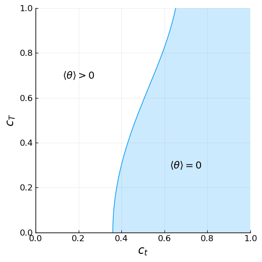
Figure 1: Phase diagram of the potential (72) in the $(c_{t},c_{T})$ plane, with $z_{R}/z_{0}=100$, $a_{W}=a_{B}=40$, and $a_{t}=10$. The solid blue line corresponds to $A=0$. It should be noted that in realistic models, $a_{W},a_{B}$, and $a_{t}$ will be determined by the mass relations (53), (58), and (68).

Now we compute the mass of the Higgs boson. By differentiating $V(h)$ twice, we find

$$\left(m_{h}\over v\right)^{2}={g_{5}^{4}k^{2}\over 32\pi^{2}}\left[B+\left(-\log{v^{2}\over f^{2}}-{3\over 2}\right)C\right]\ .$$ (73)

The quartic term in the Higgs potential originates from the box diagrams of the top and top partner, so we naturally have a factor of $g_{5}^{4}$ in this expression. Composite Higgs models typically predict a quartic term smaller than what is required for the observed Higgs mass; however, from (73), we can see how our model can overcome the challenge. First, the quadratic terms of the Higgs potential from $\Psi_{t}$ and $\Psi_{T}$ cancels each other, but their quartic terms add. Therefore, we can tune $A$ near zero without sacrificing the quartic term $B$ and $C$. Second, we can push $g_{5}$ to a larger value. As shown in (48), the gauge boundary kinetic term gives us freedom to fit the correct $SU(2)$ coupling even with a large $g_{5}$. Third, some choices of the $SO(5)$ representation for $\Psi_{T}$ can make a relatively large contribution to $B$. This is indeed the case for the $\Psi_{T}$ in the 5 of $SO(5)$. See Appendix F for details.

We can obtain a futher insight of the parameter space of our model by studying the relationship between the Higgs mass and the top quark mass. In Appendix F, we argue that near the phase transition line $A=0$, the coefficients $B$ and $C$ can be estimated as

$$B\sim{3\over 4}A_{t}(c_{t},a_{t}),\qquad C\sim 0\ ,$$ (74)

where $A_{t}$ is the quadratic term of the top quark contribution to the Higgs potential, defined in (255). Then, from (68) and (73), we have

$$\left(m_{h}\over m_{t}\right)^{2}\sim{g_{5}^{2}k\over 4\pi^{2}}\cdot\left[{L_{t}(c_{t},a_{t})\over 1+2c_{t}}\left(z_{0}\over z_{R}\right)^{1/2-c_{t}}\right]\cdot{3\over 4}A_{t}(c_{t},a_{t})\,.$$ (75)

The term in bracket and ${3\over 4}A_{t}(c_{t},a_{t})$ depend strongly on $c_{t}$ and $a_{t}$, but their product turns out almost constant across a wide range of $c_{t}$ and $a_{t}$. Numerically, for $0.3<c_{t}<0.7$ and $0<a_{t}<20$, the product stays within the interval $1.2-1.5$. This is actually to be expected, since there is a positive correlation between the top quark Yukawa coupling and its contribution to the Higgs potential.

Then the mass ratio (75) gives a rough estimate of the required value of RS coupling $g_{5}$ in our model. With this determined, we choose the size of the gauge boundary kinetic term $L_{W}$ which fits the $W$ boson mass. Using 1.3 for the value of the product in (75), we have

$$g_{5}^{2}k\sim 22\quad\textrm{and}\quad L_{W}\sim 51\ .$$ (76)

This shows that $g_{5}$ and $L_{W}$ are pushed to large values in our model. The full numerical study agrees well with this result. It gives $L_{W}$ between $35-55$ for $0.4<c_{t}<0.7$ and 1.5 TeV $<k_{R}<$ 3 TeV.

The large value of $g_{5}$ results from the relatively small quartic term $B$ of the Higgs potential. It is possible to increase $B$ by decreasing $c_{t}$, but this also decreases the term in bracket in (75), so that the value of $g_{5}$ stays large across the entire parameter space. This tension can be relaxed if there is an additional, large source of the Higgs quartic term. This will also relieve the degree of fine-tuning in our model. In [21], we showed that there are fermion gauge multiplets that can provide a positive contribution to the quartic term in the potential without affecting the quadratic term. Perhaps adding such a multiplet here will provide a more attractive set of model parameters.

5.2 Allowed region of parameter space

Now we study our parameter space with a full numerical treatment. There are nine parameters in our theory,

$$z_{0},\,z_{R},\,c_{t},\,c_{T},\,g_{5},\,g_{X},\,a_{W},\,a_{B},\,a_{t}\ ,$$ (77)

or, keeping $k_{R}=1/z_{R}$ as the only dimensionful parameter, we have

$$k_{R}\quad\textrm{and}\quad z_{R}/z_{0},\,c_{t},\,c_{T},\,g_{5}^{2}k,\,g_{X}^{2}k,\,a_{W},\,a_{B},\,a_{t}\ .$$ (78)

These parameters should produce correct values of the five independent observables,

$$G_{F} = 1.166\times 10^{-5}\,\textrm{GeV}^{-2},\quad m_{t}=147\ \textrm{GeV,}$$ (79)

$$\hskip-50.58878ptm_{W}=80.4\ \textrm{GeV,}\quad m_{Z}=91.2\ \textrm{GeV,}\quad m_{h}=125\ \textrm{GeV.}$$

We can also consider these quantities as one dimensionful observable $v$ and four dimensionless number, $e,g,y_{t}$, and $m_{h}/v$.

It is easiest to think of this parameter space as parametrized by the KK scale (a few times $k_{R}$) and the ratio $z_{R}/z_{0}$. This latter ratio is constrained by flavor physics, since light flavors will couple to the Higgs sector at the UV boundary. Flavor structure is beyond the scope of this paper, so for the moment we propose $z_{R}/z_{0}=100$.

Furthermore, we can expect from the small hypercharge coupling that $a_{B}$ should have little effect on the Higgs potential. This is indeed numerically observed. Therefore, we will assume $a_{B}=a_{W}$ throughout the rest of our analysis. This leaves us effectively a 2-dimensional parameter space.

Our strategy to find the available parameter space is as follows. We first choose values of $(c_{t},a_{t})$. Then, $m_{W}/m_{t}$ determines $a_{W}$ by (53) and (68), and $(g,e)$ determine $(g_{5}^{2}k,g_{X}^{2}k)$ by (48) and (62). With those parameters fixed, the potetial minimum is now determined by $c_{T}$. We search for the value of $c_{T}$ which gives the observed value of $m_{h}$. Although in the analysis above we have used the small $s$ expansion of the Higgs potential, our numerical analysis is conducted with the full potential before the expansion. The minimum of the full potential differs by about 10% compared to that obtained from the approximate formulae (72).

Figure 2 shows the allowed region of parameter space in the $(c_{t},a_{t})$ plane for different values of $k_{R}$. Note that parameters do not depend strongly on $k_{R}$. This implies that $k_{R}$ can be seen as one of the orthogonal directions of our two-dimensional parameter space and we can consider its effect on observables separately from other parameters. In the following analysis, we choose $c_{t}$, which represents the degree of compositeness of the top quark, as the other main variable of our parameter space. We show how physical quantities change as we vary $c_{t}$ at values of $k_{R}=1.5-3$ TeV.

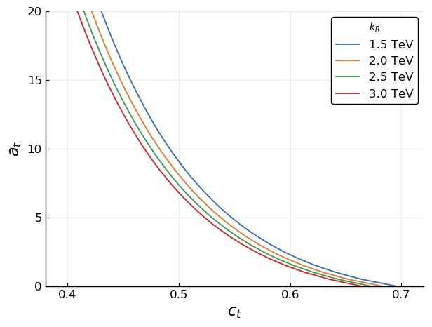
Figure 2: Allowed region of parameter space in the $(c_{t},a_{t})$ plane. Here $\Psi_{T}$ is not charged under $SU(3)_{C}$.

5.3 Mass spectrum of the top partner

The masses of new particles beyond the SM are determined by $k_{R}$. Before looking at the masses of new states in our theory, it is instructive to study masses of generic KK states in RS models. For $z_{R}/z_{0}=100$, the first KK masses of a gauge field (or a fermion with $c=1/2$) with different boundary conditions are

b.c. $$(++)$$

2.8 0.72 2.4 3.8

(80)

The UV boundary kinetic term supresses the masses of $(++)$ and $(+-)$ states, but only slightly. It has no effect on $(-+)$ and $(--)$ states. Therefore, except for the $(+-)$ state, the masses of new states will be a few times $k_{R}$. In our model, those heavy states correpsond to $Z^{\prime}$ and KK states of $W$, $B$ and the top quark. For $k_{R}>$ 1.5 TeV, these particles have masses above 4 TeV. At the lower end of this range, we must still consider the observability of these states in LHC Drell-Yan measurements. However, the KK vector bosons are IR-dominated and have suppressed couplings to light fermions associated with UV zero modes. Compared to a sequential $W^{\prime}$ and $Z^{\prime}$, the suppression is a factor of 4 in the couplings, or more when the KK boson has a UV boundary kinetic term, and this suppression factor is squared in the cross section formula. Therefore, these KK resonances are not yet constrained by LHC searches [36, 37].

On the other hand, the $(+-)$ states in the top partner multiplet $\Psi_{T}$ can have a mass lower than $k_{R}$. The dashed lines in Fig. 3 show the masses of the top partner for different values of $c_{t}$ and $k_{R}$. Searches for a vectorlike top partner at the LHC currently put the mass of this particle above 1.37 TeV [38] and thus constrains our model for $k_{R}<3$ TeV.

The LHC search assumes that the top partner is charged under $SU(3)_{C}$ and can decay into the top or bottom quark. However, whether the $\Psi_{T}$ in our model is colored or not is a model-building choice and we can proceed in either way, as long as $\Psi_{T}$ can compete with the top quark and generate the correct Higgs potential. In terms of the experimental constraints, it is much more attractive to assume that $\Psi_{T}$ is a singlet under $SU(3)_{C}$ and its states are heavy leptons: The strongest current experimental bound on a new heavy lepton is 560 GeV, in a particularly optimistic scenario [39].

The hypothesis that $\Psi_{T}$ is a color-singlet has much in common with the idea of “neutral naturalness” put forward in [40, 41]. In both cases, the Higgs potential obtains competing contributions from the top quark multiplet and from color-singlet mirror states at the TeV scale. However, conventionally in this framework, a discrete symmetry between these multiplets is used to make the one-loop contributions to the Higgs potential finite, and then further fine-tuning is needed to achieve a small value of $v/f$. Here, the finiteness of the Higgs potential is insured by the RS structure, so there is no need for mirror symmetry; however, we still need to tune $v/f$ to a small value.

The solid lines in Fig. 3 show the mass of the lightest KK state from $\Psi_{T}$ in the case where $\Psi_{T}$ is a color singlet. Without the multiplicity from color in $V_{T}$, we need to lower the value of $c_{T}$ for the correct tuning of $\Psi_{T}$ against $\Psi_{t}$ to come close to $A\sim 0$ in the Higgs potential. This leads to larger values of $m_{T}$. We find $m_{T}>820$ GeV for $k_{R}\geq 1.5$ TeV, so that in this case $k_{R}$ is unconstrained by LHC searches. In the rest of our analysis, we will use the parameter space of the uncolored $\Psi_{T}$.

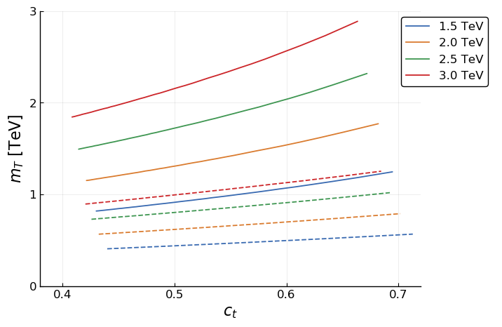
Figure 3: Masses of lightest top partner from the multiplet $\Psi_{T}$. Dashed lines correpond to color triplet $\Psi_{T}$, and solid lines correspond to color singlet $\Psi_{T}$.

5.4 Measure of fine tuning

In the composite Higgs literature, it is customary to use $\epsilon=v^{2}/f^{2}$ to quantify the degree of fine-tuning. However, at least in the class of theories where the Higgs potential is generated dynamically, $v/f$ is only a derived quantity which is determined by more fundamental parameters in the theory. In our model, those parameters are $c_{t}$ and $c_{T}$. The little hierarchy $v/f\ll 1$ requires $c_{t}$ and $c_{T}$ to be fine-tuned near the line of phase transition, as illustrated in Fig. 1. Therefore, we propose to use $\Delta c_{T}=c_{T}-c_{T,critical}$ as the measure of fine-tuning, where $c_{T,critical}$ is the value of $c_{T}$ on the phase transition line $A=0$. Fig. 4 shows the value of $\Delta c_{T}$ for varying $c_{t}$ and $k_{R}$. It should be noted that this choice does not soften the fine-tuning. For completeness, we also include a plot of $v^{2}/f^{2}$ in Fig. 5.

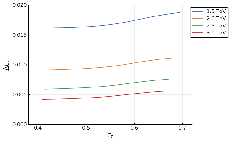
Figure 4: Values of the fine-tuning measure $\Delta c_{T}=c_{T}-c_{T,critical}$ for varying $c_{t}$ and $k_{R}$.

Figure 5: Values of $v^{2}/f^{2}$ for varying $c_{t}$ and $k_{R}$.

6 Precision electroweak observables

One of the constraints on the parameter space of RS models is that from precision electroweak measurements. The strongest of these are represented by constraints on the values of the oblique parameters $S$ and $T$ [22]. We have already invoked the small size of the $T$ parameter to require a symmetry-breaking pattern with a custodial $SU(2)$ symmetry. Beyond this, the $S$ parameter, which is a measure of the total size of the new physics correction to $W$ and $Z$ vacuum polarization functions, places a lower bound on the KK scale $k_{R}=z_{R}^{-1}$.

6.1 Simplified $S$ and $T$

Our discussion of the oblique parameters will be simplified in several respects. We will concentrate on observables involving either no external fermions or only external light leptons. In this analysis, we will ignore all masses of light leptons and assign these particles to appropriate zero modes in the ${\bf 5}$ of $SO(5)$. We will assume that all of these zero modes are UV-dominated, that is, $c>1/2$ for left-handed leptons and $c<-1/2$ for right-handed leptons. Realistic models might have different assignments, especially for the right-handed components of the quarks and leptons. We will discuss other possibilities in [24].

RS models contain additional vector bosons beyond the SM gauge bosons $\gamma$, $W^{\pm}$, and $Z$. Thus, strictly, an analysis in terms of the two parameters $S$ and $T$ does not capture the full complexity of the new physics corrections to precision electroweak formulae, even to leading order. Here, we use simplified formulae for $S$ and $T$ that capture the constraints from the five best measured observables: $\alpha(m_{Z}^{2})$, $G_{F}$, $m_{Z}$, $m_{W}$, and $s_{*}^{2}$, the effective value of $s_{w}^{2}$ at the $Z$ pole. It is shown in [42] that such an approach can put meaningful constraints on new physics even in models with additional heavy vector bosons.

In this discussion, we define $\Delta A$ to be the new physics contribution to an observable $A$. We define $\delta A$ to be the fractional deviation from the SM prediction: $\delta A=\Delta A/A$.

The $S$, $T$ formalism defines a reference weak mixing angle $\theta_{0}$ by

$$\sin^{2}2\theta_{0}=4s_{0}^{2}c_{0}^{2}={4\pi\alpha(m_{Z}^{2})\over\sqrt{2}G_{F}m_{Z}^{2}}$$ (81)

and then expresses the values of additional electroweak observables in terms of $s_{0}^{2}$ and the oblique parameters. In this approach,

$$m_{W}^{2}/m_{Z}^{2}-c_{0}^{2} = {\alpha c_{0}^{2}\over c_{0}^{2}-s_{0}^{2}}(-\frac{1}{2}\,S+c_{0}^{2}\,T)$$

$$s_{*}^{2}-s_{0}^{2} = {\alpha\over c_{0}^{2}-s_{0}^{2}}({1\over 4}\,S-s_{0}^{2}c_{0}^{2}\,T)$$ (82)

In the current situation, values of $S$ and $T$ are mainly determined by the five observables [43]. Then we can find convenient formulae representing the measured values of the oblique parameters by solving (82) for $S$ and $T$. Choose a reference set of parameters which, in zeroth order, satisfies the SM relations and let $\Delta A$ (and $\delta A=\Delta A/A$) represent the deviation of observables from the predictions at this parameter set. Then

$$\alpha\,S = 4\biggl{[}\Delta s_{*}^{2}+s_{0}^{2}(\delta m_{W}^{2}+\delta G_{F}-\delta\alpha)\biggr{]}$$

$$\alpha\,T = \biggl{[}(\delta m_{W}^{2}+s_{0}^{2}\delta G_{F})/c_{0}^{2}-\delta m_{Z}^{2}+(2\Delta s_{*}^{2}-s_{0}^{2}\delta\alpha)/c_{0}^{2}\biggr{]}\ .$$ (83)

As a check, note that, if the only corrections to precision electroweak come in a $q^{2}$-independent correction to the $W$ mass (which also affects $G_{F}$), then these formulae predict $\alpha S=0$ and $\alpha T=\delta m_{W}^{2}-\delta m_{Z}^{2}$, as desired.

In the next few subsections, we compute the tree-level ${\cal O}(s^{2})$ corrections to the five observables within our model. We will discuss the most important loop-level corrections in Section 6.5.

6.2 $\alpha(m_{Z})$, $m_{W}$, $m_{Z}$

We take (62) to provide the reference values of coupling constants and express dimensionful parameters in terms of the mass scale $s^{2}/z_{R}^{2}$. We then expand the expressions for observables in powers of $s^{2}$ around this reference point. We have seen in Section 4 that, in zeroth order, the observables satisfy the SM relations. Then $S$, $T$ computed from (83) will be of order $s^{2}$. In the discussion of this section, we will keep terms only to order $s^{2}$ and we will also ignore terms of order $z_{0}^{2}/z_{R}^{2}$.

For the electromagnetic coupling, the reference formula in (62) gives the exact value at the tree level; there are no ${\cal O}(s^{2})$ corrections. So

$$\delta\alpha=0\ .$$ (84)

Solving for zeros of the expressions (52), (57) to one higher order in $s^{2}$, we find the corrections to (53), (58)

$$\delta m_{W}^{2} = +{s^{2}\over 8L_{W}^{2}}(3L_{W}-2)={m_{W}^{2}z_{R}^{2}\over 4}\,\biggl{[}{3\over 2}-{1\over L_{W}}\biggr{]}$$

$$\delta m_{Z}^{2} = +{s^{2}\over 8L_{B}^{2}L_{W}^{2}}\,\bigl{(}3L_{B}L_{W}(L_{B}+s_{\beta}^{2}L_{W})-2(L_{B}^{2}+s_{\beta}^{2}L_{W}^{2})\bigr{)}$$ (85)

$$= {m_{Z}^{2}z_{R}^{2}\over 4}\biggl{[}{3\over 2}-\bigl{(}{c_{w}^{2}\over L_{W}}+{s_{w}^{2}\over L_{B}}\bigr{)}\biggr{]}\ .$$

These shifts in $m_{W}^{2}$ and $m_{Z}^{2}$ imply that their contributions to the $T$ parameter largely cancel. The residue is

$$\alpha\,T\biggr{|}_{m_{W}^{2},m_{Z}^{2}}=-{s_{w}^{2}m_{Z}^{2}z_{R}^{2}\over 4}({1\over L_{W}}-{1\over L_{B}})$$ (86)

and this entirely vanishes if $L_{W}=L_{B}$ or $a_{W}=a_{B}$.

6.3 $G_{F}$

To compute $G_{F}$, we consider the matrix element for muon decay $\mu\to\nu_{\mu}e\overline{\nu}_{e}$. This is computed from matrix elements of the $A_{m}^{A}$ propagators between zero mode wavefunctions. At first sight, it seems that the only contribution comes from the matrix element of $\left\langle{A^{1L}_{m}(z)A^{1L}_{n}(z^{\prime})}\right\rangle$ taken between simple left-handed zero modes for $\mu_{L}$, $\nu_{\mu L}$, $e_{L}$, $\nu_{eL}$. The Green’s function in $(z,z^{\prime})$ is integrated over the two sets of fermion zero mode wavefunctions in $z$ and $z^{\prime}$. This Green’s function is given by the result (219) derived in Appendix D.1,

$$\left\langle{A_{m}^{1L}(z)A_{n}^{1L}(z^{\prime})}\right\rangle=-\eta_{mn}{kz_{R}^{2}\over s^{2}}\left(1-{s^{2}\over 2}\left(1-{z_{<}^{2}\over z_{R}^{2}}\right)\right)\ ,$$ (87)

where $z_{<}$ is the smaller of $z$, $z^{\prime}$ under the integrals. We would find $G_{F}$ as the matrix element of this expression multiplied by the coupling constant $g_{5}^{2}/2$. Note that the ${\cal O}(s^{2})$ corrections depend on the form of the zero mode wavefunctions and not simply on the total normalizations times global charges.

However, there is a subtlety here. We might assign a left-handed lepton multiplet to a ${\bf 5}$ according to

$$\Psi_{e}=\left[\matrix{\pmatrix{E(-+)&\nu_{e}(++)\cr N(-+)&e_{L}(++)}\cr N^{\prime}(-+)}\right],$$ (88)

as in (22). Here we have chosen the $N$ and $N^{\prime}$ to have $(-+)$ boundary conditions so that neither has a right-handed zero mode that can combine with the $\nu_{e}$ zero mode to give a massive fermion. Nevertheless, the $U_{W}$ matrix generated by top quark condensation will have the form (156) in Appendix B, and this will mix the $\nu_{e}$ and $N^{\prime}$ fields on the UV boundary. As a result, the zero mode will be a mixture

$${(1+c)\over 2}\left|{\nu_{e}}\right\rangle+{(1-c)\over 2}\left|{N}\right\rangle-{s\over\sqrt{2}}\left|{N^{\prime}}\right\rangle\ .$$ (89)

The matrices $T^{a5}$ in (151), for $a=1,2$ have matrix elements between $\left|{\nu_{e}}\right\rangle$ and $\left|{N^{\prime}}\right\rangle$. The gauge field Green’s functions that can take advantage of these matrix elements are, at $p=0$ and to the leading order in $s$,

$$\left\langle{A_{m}^{1L}(z)A_{n}^{15}(z^{\prime})}\right\rangle = \eta_{mn}{kz_{R}^{2}\over s^{2}}{s\over\sqrt{2}}\Bigl{(}1-{z^{\prime 2}\over z_{R}^{2}}\Bigr{)}\ ,$$

$$\left\langle{A_{m}^{15}(z)A_{n}^{1L}(z^{\prime})}\right\rangle = \eta_{mn}{kz_{R}^{2}\over s^{2}}{s\over\sqrt{2}}\Bigl{(}1-{z^{2}\over z_{R}^{2}}\Bigr{)}\ .$$ (90)

The piece of the matrix element $\left\langle{A^{15}(z)A^{15}(z^{\prime})}\right\rangle$ containing the $W$ boson pole is proportional to $p^{2}/(p^{2}-m_{W}^{2})$. It vanishes at $p^{2}=0$ and so does not contribute to $G_{F}$. Assembling the pieces, including for each the square of the coefficient in (89), we find that there is a cancellation, so that $G_{F}$ is finally given by

$${4G_{F}\over\sqrt{2}}={g_{5}^{2}\over 2}{kz_{R}^{2}\over s^{2}}\biggl{[}1-{s^{2}\over 2}{\left\langle{z_{>}^{2}\over z_{R}^{2}}\right\rangle}\biggr{]}\ .$$ (91)

Then

$$\delta G_{F}=-{s^{2}\over 2}{\left\langle{z_{>}^{2}\over z_{R}^{2}}\right\rangle}\ .$$ (92)

The evaluation of $\left\langle{z_{>}^{2}/z_{R}^{2}}\right\rangle$ is discussed in Appendix C.3. It is less than 0.2 for zero modes with $c=1/2$ and exponentially suppressed for $c>1/2$. Therefore, for UV-dominated light leptons, $\delta G_{F}$ is negligible.

There is an easier way to obtain this result. Since all of the fields in $\Psi_{e}$ have the same boundary conditions in the IR, the Wilson line $U_{W}$ has no effect on the state when it is applied at the IR boundary. Then, in the IR gauge, the neutrino zero mode is purely $\left|{\nu_{e}}\right\rangle$. So, in this gauge, only the $\left\langle{A^{1L}_{m}(z)A^{1L}_{n}(z^{\prime})}\right\rangle$ matrix element contributes. Using (71), we find

$$\left\langle{A^{1L}_{m}(z)A^{1L}_{n}(z^{\prime})}\right\rangle_{IR}=-\eta_{mn}{kz_{R}^{2}\over s^{2}}\biggl{(}1-{s^{2}\over 2}{z_{>}^{2}\over z_{R}^{2}}\biggr{)}\ ,$$ (93)

and the result (92) follows immediately.

6.4 $s_{*}^{2}$

The parameter $s_{*}^{2}$ appears in the ratio of the amplitudes for $e^{+}e^{-}\to\mu^{+}\mu^{-}$ in the different helicity states. We now calculate $s_{*}^{2}$, defined by the formula

$${g_{Z}(e^{-}_{R})\over g_{Z}(e^{-}_{L})}={-2s_{*}^{2}\over 1-2s_{*}^{2}}\ ,$$ (94)

which corresponds to the tree-level SM relation.

The $Z$ couplings to the $e^{-}_{L}$ and $e^{-}_{R}$ zero modes are computed by taking the matrix element of the $Z$ propagator—or, rather, the $Z$ boson pole terms in the $(A^{3L},B,Z^{\prime},A^{35})$ propagators—between fermion zero modes. As in our discussion of $G_{F}$, it avoids some difficulty to work in the IR gauge where the zero modes are unmixed. Then the zero modes have matrix elements only with $(A^{3L},B,Z^{\prime})$, proportional to the $T^{3L}$, $Y$, and $T^{3R}$ charges as they appear in the covariant derivative (13). Furthermore, it should be noted that UV-dominated fermions have suppressed coupling to the $Z^{\prime}$, since this field has a $-$ UV boundary condition. This implies that the leading corrections to $s_{*}^{2}$ should have no explicit dependence on $T^{3R}$. We will see this explicitly below. Since $s_{*}^{2}$ depends only on the $T^{3L}$ and $Y$ charges, our result for $s_{*}^{2}$ actually holds for any assignments of $e^{-}_{L}$ and $e^{-}_{R}$ to $SO(5)$ representations.

We construct the propagators in the UV gauge and then apply (71). The three fields $(A^{3L},B,Z^{\prime})$, have $+$ boundary conditions in the IR brane. Then, following the general formula (135), all of their Green’s functions take the form

$$\left\langle{A^{A}_{m}(z)A^{B}_{n}(z^{\prime})}\right\rangle=\eta_{mn}\ kpz_{R}zz^{\prime}\biggl{[}{\bf A}^{AB}G_{+-}(z,z_{R})G_{+-}(z^{\prime},z_{R})+\cdots\bigr{]}\ .$$ (95)

The $Z$ boson pole $(p^{2}-m_{Z}^{2})$ is contained in the matrix ${\bf A}^{AB}$, and so the terms omitted in (95) contain $Z$ pole terms that include the factor $G_{++}(z,z_{R})$. This factor will appear in the matrix elements of $(A^{3L},B,Z^{\prime})$ when we convert to the IR gauge using (71), however, always with a coefficient of order $s^{2}$. Then we will need $G_{++}(z,z_{R})$ only to leading order

$$G_{++}(z,z_{R})={z_{R}\over 2z}\biggl{(}1-{z^{2}\over z_{R}^{2}}\biggr{)}\ ,$$ (96)

while we will need $G_{+-}(z,z_{R})$ to the next order,

$$G_{+-}(z,z_{R})={1\over pz}\cdot\biggl{[}1+{(pz_{R})^{2}\over 4}\biggl{(}-1+{z^{2}\over z_{R}^{2}}+2{z^{2}\over z_{R}^{2}}\log{z_{R}\over z}\biggr{)}\biggr{]}\ .$$ (97)

The calculation of the matrix ${\bf A}^{AB}$ is described in Appendix D.2. The expression for this matrix contains an overall factor

$$[\det{\bf C}]^{-1}={2p^{3}z_{0}^{2}z_{R}m_{Z}^{2}/s^{2}\over(L_{B}+L_{W}s_{\beta}^{2})}{1\over p^{2}-m_{Z}^{2}}\cdot{\cal Z}_{Z}(p^{2})\ .$$ (98)

up to corrections of higher order in $s^{2}$. The factors of $m_{Z}^{2}$ in (98) include the order $s^{2}$ corrections shown in (85).

The terms of order $p^{2}$, evaluated at the $Z$ pole, contribute corrections of order $s^{2}$ to the residue. However, ${\cal Z}_{Z}$ gives a correction to normalization factor that is common to all of the Green’s functions we will discuss, and one that cancels out of the ratio of couplings. The $(-1)$ term in (97) also contributes to the common overall factor. The $z$-dependent terms are very small for fermion zero modes that are peaked in the UV and therefore we omit this correction here. Similarly, we ignore $z^{2}/z_{R}^{2}$ in $G_{++}$. We will return to consider those terms in Section 7. Aside from these factors, we keep below all corrections of ${\cal O}(s^{2})$.

With this understanding, we can write the poles at $p^{2}=m_{Z}^{2}$ in the vector field Green’s functions. Up to terms of order $s^{2}$, we find

$$\left\langle{A^{3L}_{m}A^{3L}_{n}}\right\rangle = {k\eta_{mn}\over(p^{2}-m_{Z}^{2})(L_{B}+s_{\beta}^{2}L_{W})}\biggl{[}{L_{B}\over L_{W}}-{s^{2}\over 4}{(L_{B}+s_{\beta}^{2}L_{W})\over L_{B}L_{W}^{3}}(L_{B}-L_{W}+2L_{B}L_{W}^{2})\biggr{]}$$

$$\left\langle{A^{3L}_{m}B_{n}}\right\rangle = {k\eta_{mn}s_{\beta}\over(p^{2}-m_{Z}^{2})(L_{B}+s_{\beta}^{2}L_{W})}\biggl{[}-1+{s^{2}\over 4}{(L_{B}+s_{\beta}^{2}L_{W})\over L_{B}L_{W}}(L_{B}+L_{W})\biggr{]}$$

$$\left\langle{B_{m}B_{n}}\right\rangle = {k\eta_{mn}s_{\beta}^{2}\over(p^{2}-m_{Z}^{2})(L_{B}+s_{\beta}^{2}L_{W})}\biggl{[}{L_{W}\over L_{B}}-{s^{2}\over 4}{(L_{B}+s_{\beta}^{2}L_{W})\over L_{B}^{3}L_{W}}(L_{W}-L_{B}+2L_{B}^{2}L_{W})\biggr{]}$$

$$\left\langle{A^{3L}_{m}Z^{\prime}_{n}}\right\rangle = {k\eta_{mn}c_{\beta}\over(p^{2}-m_{Z}^{2})(L_{B}+s_{\beta}^{2}L_{W})}\biggl{[}+{s^{2}\over 4}{(L_{B}+s_{\beta}^{2}L_{W})\over L_{W}}\biggr{]}$$

$$\left\langle{B_{m}Z^{\prime}_{n}}\right\rangle = {k\eta_{mn}s_{\beta}c_{\beta}\over(p^{2}-m_{Z}^{2})(L_{B}+s_{\beta}^{2}L_{W})}\biggl{[}-{s^{2}\over 4}{(L_{B}+s_{\beta}^{2}L_{W})\over L_{B}}\biggr{]}$$

$$\left\langle{Z^{\prime}_{m}Z^{\prime}_{n}}\right\rangle = 0$$

$$\left\langle{A^{3L}_{m}A^{35}_{n}}\right\rangle = {k\eta_{mn}\over(p^{2}-m_{Z}^{2})(L_{B}+s_{\beta}^{2}L_{W})}\biggl{[}-{s\over\sqrt{2}}{(L_{B}+s_{\beta}^{2}L_{W})\over L_{W}}\biggr{]}$$

$$\left\langle{B_{m}A^{35}_{n}}\right\rangle = {k\eta_{mn}s_{\beta}\over(p^{2}-m_{Z}^{2})(L_{B}+s_{\beta}^{2}L_{W})}\biggl{[}+{s\over\sqrt{2}}{(L_{B}+s_{\beta}^{2}L_{W})\over L_{B}}\biggr{]}$$

$$\left\langle{Z^{\prime}_{m}A^{35}_{n}}\right\rangle = 0$$

$$\left\langle{A^{35}_{m}A^{35}_{n}}\right\rangle = {k\eta_{mn}\over(p^{2}-m_{Z}^{2})(L_{B}+s_{\beta}^{2}L_{W})}\biggl{[}+{s^{2}\over 2}{(L_{B}+s_{\beta}^{2}L_{W})^{2}\over L_{W}L_{B}}\biggr{]}\ .$$ (99)

The expressions factorize onto the pole of a single vector meson, as required, giving the coupling between lepton zero modes 1 and 2

$${g_{Z}(1)\ g_{Z}(2)\over p^{2}-m_{Z}^{2}}\ .$$ (100)

From these expressions, and using (62) to make some simplifications, we can write the $Z$ wavefunction in the UV gauge (for $z\ll z_{R}$) as

$$\left|{Z}\right\rangle=\left({k\over L_{W}c^{2}_{w}}\right)^{1/2}\times \Biggl{\{}c_{w}^{2}\left(1-{s^{2}\over 8}{(L_{B}+s_{\beta}^{2}L_{W})\over L_{B}^{2}L_{W}^{2}}(L_{B}-L_{W}+2L_{B}L_{W}^{2})\right)\left|{A^{3L}}\right\rangle$$ (101)

$$\hskip 21.68121pt-{s_{w}^{2}\over s_{\beta}}\left(1-{s^{2}\over 8}{(L_{B}+s_{\beta}^{2}L_{W})\over L_{B}^{2}L_{W}^{2}}(L_{W}-L_{B}+2L_{B}^{2}L_{W})\right)\left|{B}\right\rangle$$

$$\hskip 21.68121pt+c_{\beta}{s^{2}\over 4}\left|{Z^{\prime}}\right\rangle-{s\over\sqrt{2}}\left|{A^{35}}\right\rangle\Biggr{\}}\ .$$

To obtain the $Z$ wavefunction in the IR gauge, apply $U_{W}$ to this wavefunction as indicated in (71). There is a nice cancellation, and we find

$$\left|{Z}\right\rangle_{IR}=\left({k\over L_{W}c^{2}_{w}}\right)^{1/2}\times \Biggl{\{}c_{w}^{2}\left(1-{s^{2}\over 8}{(L_{B}+s_{\beta}^{2}L_{W})\over L_{B}^{2}L_{W}^{2}}(L_{B}-L_{W})\right)\left|{A^{3L}}\right\rangle$$ (102)

$$\hskip 21.68121pt-{s_{w}^{2}\over s_{\beta}}\left(1+{s^{2}\over 8}{(L_{B}+s_{\beta}^{2}L_{W})\over L_{B}^{2}L_{W}^{2}}(L_{B}-L_{W})\right)\left|{B}\right\rangle\Biggr{\}}\ .$$

with no $Z^{\prime}$ or $A^{35}$ components. Then we can read off the $Z$ coupling to a massless fermion as

$$g_{Z} = gc_{w}\biggl{[}T^{3L}\ \bigl{\{}1-{s^{2}\over 8}{(L_{B}+L_{W}s_{\beta}^{2})\over L_{B}^{2}L_{W}^{2}}(L_{B}-L_{W})\bigr{\}}$$ (103)

$$\hskip 57.81621pt-{s_{w}^{2}\over c_{w}^{2}}Y\ \bigl{\{}1+{s^{2}\over 8}{(L_{B}+L_{W}s_{\beta}^{2})\over L_{B}^{2}L_{W}^{2}}(L_{B}-L_{W})\bigr{\}}\biggr{]}\ .$$

This formula applies to any zero-mode fermion that is unmixed in the IR gauge and strongly localized in the UV. Note that it contains no separate dependence on $T^{3R}$. It is an interesting exercise to collect the extra terms that appear in the UV gauge for $(\nu,e)_{L}$ in the ${\bf 5}$ and also in the ${\bf 4}$ and see how the $T^{3R}$ terms cancel in all of these cases.

Finally, as in (86), the precision electroweak correction is proportional to $(L_{W}-L_{B})$. Computing (94), we find

$$\Delta s_{*}^{2}=(s_{*}^{2}-s_{w}^{2})={s^{2}s_{w}^{2}c_{w}^{2}\over 4L_{B}^{2}L_{W}^{2}}(L_{B}+s_{\beta}^{2}L_{W})={m_{Z}^{2}z_{R}^{2}s_{w}^{2}c_{w}^{2}\over 4}({1\over L_{W}}-{1\over L_{B}})\ .$$ (104)

6.5 Loop corrections to $T$

The formulae that we have derived so far represent the formally leading new physics corrections to $S$ and $T$. However, it has been shown in other investigations of precision electroweak corrections to composite Higgs models, that loop effects on $T$ from the top quark and top partners can also make significant contributions [22, 44, 45]. In this section, we will make an estimate of the contribution to $T$ from fermion loop effects, dealing as best we can with the non-renormalizability of this 5D theory.

We will work from the original formula for $T$ [22],

$$\alpha T={e^{2}\over s_{w}^{2}c_{w}^{2}m_{Z}^{2}}\bigl{(}\Pi_{1L,1L}(0)-\Pi_{3L,3L}(0)\bigr{)}\ ,$$ (105)

where $\Pi_{aL,aL}$ is the vacuum polarization amplitude for the currents of the $a$ component of weak isospin. The expression for $T$ in (83) involves contributions at $q^{2}=0$ and at $q^{2}=m_{W}^{2},m_{Z}^{2}$. In this section, we will simplify the calculation of the loop integral by working at $q^{2}=0$ only. We will calculate in the IR gauge, in which the contribution of $A^{a5}$ to the $W$ and $Z$ wavefunctions is, if not completely zero, at least highly suppressed.

The vacuum polarization amplitudes in (105) involve loops with the $t_{L}$ and $b_{L}$ field in $\Psi_{t}$ and the corresponding fields in $\Psi_{T}$. The currents involve only the 4D left-handed components of these fields. Then the propagators, in Euclidean space, can be written as

$$\left\langle{(t_{L})_{L}(z,p)(t_{L})_{L}^{\dagger}(z^{\prime},p)}\right\rangle = \sigma\cdot p\ {\cal S}_{t}(z,z^{\prime},p)$$

$$\left\langle{(b_{L})_{L}(z,p)(b_{L})_{L}^{\dagger}(z^{\prime},p)}\right\rangle = \sigma\cdot p\ {\cal S}_{b}(z,z^{\prime},p)\ .$$ (106)

Here the $L$ inside the parentheses labels the species in (22) while the $L$ outside the parentheses indicates a projection onto the 2-component fermion with left-handed chirality. Using (106) to evaluate the $\Psi_{t}$ contribution to $T$, we find

$$\alpha T={3e^{2}\over s_{w}^{2}c_{w}^{2}m_{Z}^{2}}\int{dz\over(kz)^{4}}{dz^{\prime}\over(kz^{\prime})^{4}}\int{d^{4}p\over(2\pi)^{4}}\ {1\over 4}p^{2}\ ({\cal S}_{t}-{\cal S}_{b})^{2}\ .$$ (107)

The integral $d^{4}p$ is over Euclidean momentum space. Note that $({\cal S}_{t}-{\cal S}_{b})$ is of order $s^{2}$, so this contribution to $T$ is of order $s^{4}$.

We proceed, then, to evaluate $T$ from the formula (107). A complete evaluation of this expression (107) is beyond the scope of this paper. Instead, we will estimate the integral from its low-momentum behavior of the integrand. The $t_{L}$ and $b_{L}$ propagators are given by their SM formulae, plus corrections of order $m_{t}z_{R}$ and $pz_{R}$. We can write these as

$${\cal S}_{t} = f_{L}(c)^{2}(zz^{\prime})^{2-c}\cdot{1\over p^{2}+m_{t}^{2}}\biggl{[}1+A\,(m_{t}z_{R})^{2}+B\,(pz_{R})^{2}+\cdots\biggr{]}$$

$${\cal S}_{b} = f_{L}(c)^{2}(zz^{\prime})^{2-c}\cdot{1\over p^{2}}\biggl{[}1+C\,(pz_{R})^{2}+\cdots\biggr{]}\ .$$ (108)

The first factor is the form of the zero mode wavefunctions as functions of $z$ and $z^{\prime}$; see (200). The correction terms are summarized in coefficients $A$, $B$, $C$. These coefficients may contain additional dependence on $z$, $z^{\prime}$. To linear order in the coefficients, this is treated by taking the expectation values of the $z$, $z^{\prime}$-dependent terms as indicated by the $dz$ integrals.

Using (108), the $d^{4}p$ integral in (107) becomes

$$\int{d^{4}p\over(2\pi)^{4}}\ p^{2}\ \biggl{[}{m_{t}^{4}\over p^{4}(p^{2}+m_{t}^{2})^{2}}-2A{m_{t}^{4}z_{R}^{2}\over p^{2}(p^{2}+m_{t}^{2})^{2}}$$ (109)

$$\hskip 50.58878pt-2B{m_{t}^{2}z_{R}^{2}\over(p^{2}+m_{t}^{2})^{2}}+2C{m_{t}^{2}z_{R}^{2}\over p^{2}(p^{2}+m_{t}^{2})}+\cdots\biggr{]}$$

The integral of the first term is convergent. This is proportional to $m_{t}^{4}/m_{t}^{2}$ and so actually of order $s^{2}$ due to the infrared behavior of the integral. The integrals of the correction terms give cutoff-dependent contributions of order $m_{t}^{4}z_{R}^{2}$. Higher-order terms in $p^{2}$ in (108) also contribute at this order, and we expect that the sum leads to an expression that is at worst log divergent in the ultraviolet. But these terms in the integral also contain infrared-enhanced terms of order $m_{t}^{4}z_{R}^{2}\log(1/m_{t}^{2})$. Using either dimensional regularization or an explicit cutoff on the integral, we find

$$\alpha T=\alpha\cdot{3m_{t}^{2}\over 16\pi s_{w}^{2}c_{w}^{2}m_{Z}^{2}}\biggl{[}1+2\,(2B-A-C)\,m_{t}^{2}z_{R}^{2}\,\log(\Lambda^{2}/m_{t}^{2})\ +\ {\cal O}(m_{t}^{2}z_{R}^{2})\biggr{]}\ ,$$ (110)

where $\Lambda$ is an ultraviolet scale. There is also a contribution to $T$ from the vacuum polarization of $\Psi_{T}$, but this contains no light fermions and so contributes only the hard, non-logarithmic, term in (110). The leading term is the usual SM contribution to $T$ from the $(t,b)$ doublet. The usual convention is that $T$ parametrizes a deviation from the $SM$, so we will now drop this term. We claim that the RS contribution to $T$ can be estimated from the expression

$$\alpha T=\alpha\cdot{3m_{t}^{2}\over 16\pi s_{w}^{2}c_{w}^{2}m_{Z}^{2}}\cdot 2\,(2B-A-C)\,m_{t}^{2}z_{R}^{2}\,\log(\Lambda^{2}/m_{t}^{2})$$ (111)

by ignoring the hard corrections and varying $\Lambda$ over the interval $1/z_{R}$ to $1/z_{0}$.

The complete expressions for the coefficients $A$, $B$, $C$ in the IR gauge are given in Appendix G. In the parameter discussion in Section 5, we found that the top quark boundary kinetic term $a_{t}$ and the related value $L_{t}=G_{t--}(z_{0},z_{R})$ must be large. Then we can simplify the full expression for our estimate by keeping only the terms leading in $a_{t}$. This gives the relatively simple estimate

$$T\approx{3m_{t}^{4}z_{R}^{2}\over 16\pi s_{w}^{2}c_{w}^{2}m_{Z}^{2}}\ s^{2}\ \left\langle{({z\over z_{R}}\bigr{)}^{2c_{t}+1}+({z^{\prime}\over z_{R}}\bigr{)}^{2c_{t}+1}}\right\rangle\log(\Lambda^{2}/m_{t}^{2})\ ,$$ (112)

where the indicated expectation value is taken in the zero mode wavefunction using the measure (205). However, because the indicated expectation values of $z$ and $z^{\prime}$ are small, this parametrically dominant term is not actually larger than the other pieces, so we quote it here mainly for illustration. The full result for our estimate of $T$ is given in Appendix G in (278).

6.6 Phenomenological implications

We must now sum all of these contributions as indicated in (83). We may omit the small correction $\delta G_{F}$. Then, for $S$

$$\alpha S=m_{Z}^{2}z_{R}^{2}s_{w}^{2}c_{w}^{2}\biggl{(}{3\over 2}-{1\over L_{B}}\biggr{)}\ .$$ (113)

For large $L_{B}$ as is found in the parameter space of Section 5, a limit of $S<0.135$ gives the constraint

$$k_{R}>1.5~{}\mbox{TeV}\ .$$ (114)

For $T$, we find the tree-level RS correction

$$\alpha T={m_{Z}^{2}z_{R}^{2}s_{w}^{2}\over 4}\biggl{[}{1\over L_{W}}-{1\over L_{B}}\biggr{]}$$ (115)

plus the loop correction estimated by (112).

Fig. 6 shows the mapping of our parameter space onto the region of $S$ and $T$ allowed by experiment [43]. In view of the uncertainties in our estimate of the $T$ parameter, we regard the parameter region of our model with $k_{R}>1.5$ TeV to be in reasonable agreement with the current values of the precision electroweak observables.

Figure 6: Corrections to $S,T$ parameters of our model. The inner and outer contours are for 68% and 95% confidence level, respectively, from [43]. The black error bar at the origin corresponds to current top quark mass uncertainty. Each colored line represents the estimated range of $T$ parameter by varying the cutoff $\Lambda$ from $k_{R}$ to $k$.

7 $Z\to b\overline{b}$

In the analysis of the coupling of the $Z$ to fermions, we assumed that all of the relevant quarks and leptons are associated with fermion zero modes that are highly peaked in the UV. However, this is not the case for the $b$ quark. The $b_{L}$ is the $SU(2)$ partner of the $t_{L}$, and so it must share the same value of $c$. For $b_{R}$, the story is somewhat more involved. The $b_{R}$ zero mode is not included in either of the multiplets $\Psi_{t}$, $\Psi_{T}$ that we have considered so far in our analysis. However, models for generating the $b$ quark mass typically require $b_{R}$ to have a positive value of $c$, pushing the zero mode wavefunction to the IR and potentially giving large effects [24]. In this section, we provide general formulae for the special influence of the $b$ quark zero modes on the relevant precision electroweak observables. As in our discussion of $\Delta s_{*}^{2}$, we will not need to assume the particular model studied in Section 5, because we will work from the simple, general formulae for $Z$ boson couplings derived in Section 6.4.

The $b$ quark couplings to the $Z$ boson are tested with precision by the ratio of yields

$$R_{b}={\Gamma(Z\to b\overline{b})\over\Gamma(Z\to\mbox{hadrons})}$$ (116)

and the polarization asymmetry

$$A_{b}={\Gamma(Z\to b_{L}\overline{b}_{R})-\Gamma(Z\to b_{R}\overline{b}_{L})\over\Gamma(Z\to b_{L}\overline{b}_{R})+\Gamma(Z\to b_{R}\overline{b}_{L})}$$ (117)

Looking back at the discussion following (98), we see that the factor ${\cal Z}_{Z}$ cancels out of both ratios, while $z$-depdendent terms in $G_{+-}(z,z_{R})$ and $z^{2}/z_{R}^{2}$ in $G_{++}(z,z_{R})$ will make a contribution if the zero mode wavefunction extends into the IR. Including those factors, the $Z$ wavefunction in the IR gauge can be written as

$$\left|{Z}\right\rangle_{IR} = \left({k\over L_{W}c^{2}_{w}}\right)^{1/2}$$ (118)

$$\times\Biggl{\{}c_{w}^{2}\left[1+{m_{Z}^{2}z_{R}^{2}\over 4}\left(-{1\over 2L_{W}}+{1\over 2L_{B}}+(1-2L_{W}){z^{2}\over z_{R}^{2}}+2{z^{2}\over z_{R}^{2}}\log{z_{R}\over z}\right)\right]\left|{A^{3L}}\right\rangle$$

$$\hskip 21.68121pt-{s_{w}^{2}\over s_{\beta}}\left[1+{m_{Z}^{2}z_{R}^{2}\over 4}\left({1\over 2L_{W}}-{1\over 2L_{B}}+(1-2L_{B}){z^{2}\over z_{R}^{2}}+2{z^{2}\over z_{R}^{2}}\log{z_{R}\over z}\right)\right]\left|{B}\right\rangle$$

$$\hskip 21.68121pt+c_{w}^{2}c_{\beta}{m_{Z}^{2}z_{R}^{2}\over 4}\cdot 2L_{W}{z^{2}\over z_{R}^{2}}\left|{Z^{\prime}}\right\rangle+c_{w}{m_{Z}z_{R}\over 2}\cdot\sqrt{2L_{W}}{z^{2}\over z_{R}^{2}}\left|{A^{35}}\right\rangle\Biggr{\}}\ .$$

The $A^{35}$ contribution will be utimately suppressed by $m_{b}^{2}z_{R}^{2}$. Then the correction to the coupling of $Z$ boson to the bottom quark is given by

$$\Delta g_{Zb} = gc_{w}\cdot{m_{Z}^{2}z_{R}^{2}\over 4}\times\Biggl{\{}(T^{3L}-{s_{w}^{2}\over c_{w}^{2}}Y)\left\langle{2{z^{2}\over z_{R}^{2}}\log{z_{R}\over z}+{z^{2}\over z_{R}^{2}}}\right\rangle$$ (119)

$$\hskip 36.135pt+(T^{3L}+{s_{w}^{2}\over c_{w}^{2}}Y)\left({1\over 2L_{B}}-{1\over 2L_{W}}\right)+2L_{W}\left\langle{{z^{2}\over z_{R}^{2}}}\right\rangle(-T^{3L}+T^{3R})\Biggr{\}}$$

$$= g_{Zb}\cdot{m_{Z}^{2}z_{R}^{2}\over 4}\left(\left\langle{2{z^{2}\over z_{R}^{2}}\log{z_{R}\over z}+{z^{2}\over z_{R}^{2}}}\right\rangle+2L_{W}\left\langle{{z^{2}\over z_{R}^{2}}}\right\rangle{-T^{3L}+T^{3R}\over T^{3L}-(s_{w}^{2}/c_{w}^{2})Y}\right)\,.$$

where $g_{Zb}$ is the SM $Z$ coupling to $b_{L}$ or $b_{R}$ and the expectation value of $z$ must be computed in the appropriate zero mode wavefunction. Note that in the final line we omitted the terms suppressed by $1/L_{W,B}$.

The second term in (119) is enhanced by a large $L_{W}$ and can cause a large deviation in $g_{Zb}$. However, specifically for $\Psi_{t}$ in the 5 representation of $SO(5)$, we have $T^{3L}=T^{3R}=-1/2$ for $b_{L}$, and the $L_{W}$-enhanced term in (119) vanishes identically. This shows that the custodial symmetry proposed in [33] to protect the $Zbb$ vertex is working correctly. Although the formula (119) is a general result which applies to any assignment of $b$ quark in $SO(5)$, we focus on the 5 representation in the remaining of this section and study whether the remaining correction in $g_{Zb}$ gives constraints on the parameter space.

For the case of a $(t_{L},b_{L})$ doublet in 4 as in (21), the $L_{W}$-enhanced term will give a dominant correction to $g_{Zb}$. Such models can still be viable for higher values of $k_{R}$ or for assignments of both $b_{L}$ and $b_{R}$ to UV-dominated zero modes [24].

For the evaluation of (119), the computation of the $z$ expectation values is discussed in Appendix C.3. For a left-handed zero mode with positive $c$, taking $a=0$ for reference,

$$\left\langle{2{z^{2}\over z_{R}^{2}}\log{z_{R}\over z}+{z^{2}\over z_{R}^{2}}}\right\rangle=(0.36,0.11,0.047)$$ (120)

for $c=(0.3,0.5,0.7)$ and $z_{0}/z_{R}=0.01$. The value is exponentially decreasing with increasing $c$. For a right-handed zero mode with positive $c$, we find

$$\left\langle{2{z^{2}\over z_{R}^{2}}\log{z_{R}\over z}+{z^{2}\over z_{R}^{2}}}\right\rangle={(1+2c)(5+2c)\over(3+2c)^{2}}=(0.69,0.75,0.79)$$ (121)

for $c=(0.3,0.5,0.7)$.

The $b_{L}$ and $b_{R}$ $Z$ couplings have different effects on $R_{b}$ and $A_{b}$ due to the very different sizes of these couplings,

$${g_{ZbR}^{2}\over g_{ZbL}^{2}}=0.0331\ .$$ (122)

The correction to $R_{b}$ is dominated by the shift of $g_{ZbL}$,

$$\Delta R_{b}\approx 2R_{b}(1-R_{b})\bigl{[}\delta g_{ZbL}+{g_{ZbR}^{2}\over g_{ZbL}^{2}}\delta g_{ZbR}\bigr{]}\ .$$ (123)

Then

$$\Delta R_{b} \approx \frac{1}{2}R_{b}(1-R_{b})\cdot m_{Z}^{2}z_{R}^{2}\left\langle{2{z^{2}\over z_{R}^{2}}\log{z_{R}\over z}+{z^{2}\over z_{R}^{2}}}\right\rangle_{L}$$ (124)

$$= (3.7\times 10^{-4})\left\langle{2{z^{2}\over z_{R}^{2}}\log{z_{R}\over z}+{z^{2}\over z_{R}^{2}}}\right\rangle_{L}\ .$$

The last line here is evaluated using the limit in (114) for $z_{R}$. The expectation value is to be taken in the $b_{L}$ zero mode wavefunction.

On the other hand, the correction to $A_{b}$ comes equally from $g_{ZbL}$ and $g_{ZbR}$,

$$\Delta A_{b}\approx 4{g_{ZbR}^{2}\over g_{ZbL}^{2}}\,(\delta g_{ZbL}-\delta g_{ZbR})\ .$$ (125)

Then

$$\Delta A_{b} \approx {g_{ZbR}^{2}\over g_{ZbL}^{2}}m_{Z}^{2}z_{R}^{2}\biggl{(}\left\langle{2{z^{2}\over z_{R}^{2}}\log{z_{R}\over z}+{z^{2}\over z_{R}^{2}}}\right\rangle_{L}-\left\langle{2{z^{2}\over z_{R}^{2}}\log{z_{R}\over z}+{z^{2}\over z_{R}^{2}}}\right\rangle_{R}\biggr{)}$$ (126)

$$\approx -(1.4\times 10^{-4})\left\langle{2{z^{2}\over z_{R}^{2}}\log{z_{R}\over z}+{z^{2}\over z_{R}^{2}}}\right\rangle_{R}\ .$$

where again we used (114) for $z_{R}$. The expectation value in the last line is to be taken in the $b_{R}$ zero mode wavefunction, which, to obtain as large as possible a value of $\Delta A_{b}$, would be larger than the corresponding expectation value for $b_{L}$.

The experimental measurements of these quantities are [46]

$$R_{b}=0.216\pm 0.00066\,,\quad A_{b}=0.923\pm 0.020$$ (127)

so the predicted deviations from this class of RS models are well within the errors. Although it is typical in composite Higgs models that the experimental measurement of $R_{b}$ places a very strong constraint, that is not true with the custodial symmetry protecting the $Zbb$ vertex.

8 Conclusions

In this paper, we developed and examined a realistic model of a composite Higgs boson based on the gauge-Higgs unification framework and $SO(5)\times U(1)$ gauge symmetry. The top quark multiplet $\Psi_{t}$ triggers electroweak symmetry breaking. A new Dirac fermion $\Psi_{T}$ competes with the top quark and allows us to tune the value of the Higgs boson (mass)² term. We can achieve the hierarchy $v/f\ll 1$ by arranging the 5D mass parameters of the top quark and top partner to be close to the second-order phase transition in the plane of these parameters. We also introduced UV boundary kinetic terms for the gauge fields and top quark, which give us the freedom to fit the $SU(2)$ gauge coupling and the top quark Yukawa coupling.

After applying constraints from the $W$, $Z$, $t$, and Higgs masses, our model has an effectively two-dimensional parameter space. We computed the full Higgs potential and studied the allowed region in this space. It turns out that our minimal model requires large values for the UV boundary terms. An additional source of the quartic term in the Higgs potential could relax the tension that leads to these large terms.

Our model is not strongly constrained by current experimental results. Although the mass of the top partner $\Psi_{T}$ is significantly smaller than the scale of the new composite sector, we can avoid constraints from LHC searches if $\Psi_{T}$ is color-neutral. This solution is similar to the idea of “neutral naturalness” but is distinct in important respects. The main constraint on our parameter space comes from precision electroweak measurements. To analyze this constraint, we use the small value of $v/f$ required in our model as an expansion parameter. This strategy allows us to write general formulae for the precision electroweak corrections due to the new composite sector. A lower limit on the RS scale of 1.5 TeV allows our model to be consistent with current electroweak data.

In this paper, we left open the question of how the lighter quarks and leptons receive their masses. A particularly interesting question is that of how we can generate the bottom quark mass in this framework. In a forthcoming paper, we will study possible scenarios of light flavor mass generation and their implication for observable effects in $e^{+}e^{-}\to f{\overline{f}}$ processes [24].

Appendix A Properties of Minkowski-space Green’s functions

The computations done in this paper make use of Green’s functions for spin 1/2 and spin 1 fields in the RS background with Dirichlet or Neumann boundary conditions on the IR brane. The formalism for computing these Green’s functions was reviewed in [21]. However, since [21] was mainly devoted to the computation of the Coleman-Weinberg potential, the equations for Green’s functions were given for Euclidean time, and the full expressions for the Green’s functions were not needed. In this Appendix, we present the formulae for Minkowski-space Green’s functions in a notation consistent with the conventions of [21]. In this section, and in the rest of the Appendix, we will work in the UV gauge defined in Section 4.5 unless it is explicitly noted otherwise.

A.1 Building blocks

Green’s functions for fields in the RS background are built up from Bessel functions with definite boundary conditions at the UV and IR branes. In Minkowski space, we will choose as out basic building blocks the combinations $G^{(c)}_{\alpha\beta}(z_{1},z_{2},p)$, defined in (7). These functions depend on two 5th-dimension coordinates $z_{1}$, $z_{2}$, the parameter $c$, and $\alpha,\beta=\pm$. For a massive spin 1/2 field in RS, $c=m/k$. The 4-vector $p$ is the 4D momentum. When combined with a prefactor $z^{a}$, where $a=1$ for spin 1 field and $a=5/2$ for spin 1/2 fields, $G_{\alpha\beta}(z,z_{R})$ satisfies Dirichlet or Neumann boundary conditions on the IR brane at $z=z_{R}$. Typically, we will keep the dependence on $c$ and $p$ implicit. In this paper, we will work with the $G$ functions for Minkowski $p^{\mu}$, that is $p^{2}>0$, $p=(p^{2})^{1/2}$. Analogous formulae for the $G$ functions at Euclidean $p$, $p^{2}<0$, which we will denote $G_{E\alpha\beta}(z_{1},z_{2})$, are given in [21].

The $G$ functions (at fixed $c$ and $p$) manifestly satisfy

$$G_{ab}(z_{1},z_{2})=-G_{ba}(z_{2},z_{1})\ .$$ (128)

Less trivially, they satisfy the Wronskian identity

$$G_{\alpha+}(z_{1},z_{3})G_{\beta-}(z_{2},z_{3})-G_{\alpha-}(z_{1},z_{3})G_{\beta+}(z_{2},z_{3})={1\over pz_{3}}G_{\alpha\beta}(z_{1},z_{2})\ .$$ (129)

An important special case is

$$G_{++}(z_{1},z_{2})G_{--}(z_{1},z_{2})-G_{+-}(z_{1},z_{2})G_{-+}(z_{1},z_{2})={1\over p^{2}z_{1}z_{2}}\ .$$ (130)

To explore the properties of particles with masses much less than the KK scale $k_{R}$, we will need the expansions of $G_{\alpha\beta}(z_{1},z_{2})$ for small $p$. For general $c$ in the range $-1<c<1$,

$$G_{++}(p) \approx (z_{1}z_{2})^{-c-1/2}(z_{2}^{2c+1}-z_{1}^{2c+1})/(2c+1)$$

$$G_{+-}(p) \approx z_{2}^{c-1/2}z_{1}^{-c-1/2}/p$$

$$G_{-+}(p) \approx -z_{1}^{c-1/2}z_{2}^{-c-1/2}/p$$

$$G_{--}(p) \approx (z_{1}z_{2})^{-c+1/2}(z_{2}^{2c-1}-z_{1}^{2c-1})/(2c-1)\ .$$ (131)

For the special case of $c=\frac{1}{2}$,

$$G_{++}(p) \approx (z_{1}z_{2})^{-1}(z_{2}^{2}-z_{1}^{2})/2$$

$$G_{+-}(p) \approx z_{1}^{-1}/p$$

$$G_{-+}(p) \approx -z_{2}^{-1}/p$$

$$G_{--}(p) \approx \log(z_{2}/z_{1})\ .$$ (132)

A.2 Spin 1 fields

For spin 1 fields, $c=1/2$. The solutions of the gauge-fixed Maxwell equations in $z$ are $z\,G_{\alpha\beta}(z,z^{\prime})$, with $\alpha=+$ for $A^{A}_{m}$, $m=0,1,2,3$, and $\alpha=-$ for $A^{A}_{5}$. The solutions for the ghost fields also have $\alpha=+$.

We will construct solutions with definite Neumann $(+)$ or Dirichlet $(-)$ boundary conditions on the IR brane at $z=z_{R}$. The solutions to the Maxwell equation satisfying these boundary conditions contains

$$+$$ b.c. at b.c. at

(133)

For a consistent definition of $F^{A}_{m5}$ on the boundary, $A^{A}_{5}$ must satisfy $-$ boundary conditions if $A^{A}_{m}$ satisfies $+$ boundary conditions, and vice versa. We will also need to impose the condition that our solution satisfies Neumann $(+)$ or Dirichlet $(-)$ boundary conditions on the UV brane at $z=z_{0}$. These conditions are

$$+$$ b.c. at b.c. at

(134)

That is, the first index of $G$ should be appropriately raised or lowered to apply the Neumann condition.

Then the Green’s functions of spin $\frac{1}{2}$ fields are given by the following formula: For the Green’s functions of fields $A^{A}_{m},A^{B}_{n}$ obeying $\beta,\gamma$ boundary conditions on the IR brane

$$\left\langle{A^{A}_{m}(z)A^{B}_{n}(z^{\prime})}\right\rangle = \eta_{mn}\ kpz_{R}zz^{\prime}\biggl{[}{\bf A}^{AB}G_{+,-\beta}(z,z_{R})G_{+,-\gamma}(z^{\prime},z_{R})$$ (135)

$$\hskip 28.90755pt-\delta^{AB}\cases{\widetilde{G}_{+,-\beta}(z,z_{R})G_{+,-\gamma}(z^{\prime},z_{R})&$z<z^{\prime}$\cr G_{+,-\beta}(z,z_{R})\widetilde{G}_{+,-\gamma}(z^{\prime},z_{R})&$z>z^{\prime}$\cr}\biggr{]}\ ,$$

where the $\widetilde{G}$ are defined by

$$\matrix{\widetilde{G}_{++}(z,z_{R})=+G_{+-}(z,z_{R})&\widetilde{G}_{+-}(z,z_{R})=-G_{++}(z,z_{R})\cr\widetilde{G}_{-+}(z,z_{R})=+G_{--}(z,z_{R})&\widetilde{G}_{--}(z,z_{R})=-G_{-+}(z,z_{R})\cr}$$ (136)

The term in the second line of (135) satisfies the discontinuity of the Green’s function at $z=z^{\prime}$. It is present only in the diagonal correlation function. The Green’s functions of $A^{A}_{5}$ fields are constructed similarly, with $G_{+,-\beta}\to G_{-,-\beta}$.

The choice of starting from definite $+$ or $-$ boundary conditions on the IR brane comes from our convention of choosing the UV gauge, in which the Wilson line $U_{W}$ is implemented as a boundary condition on the UV brane. There is an equivalent formalism for Green’s functions in the IR gauge, in which the Wilson line is moved to the IR brane and implemented there as an IR boundary condition. In that case, we would choose definite $+$ or $-$ boundary conditions on the UV brane. The solution for the Green’s function in this case is completely analogous, starting from the formula

$$\left\langle{A^{A}_{m}(z)A^{B}_{n}(z^{\prime})}\right\rangle_{IR} = -\eta_{mn}\ kpz_{0}zz^{\prime}\biggl{[}{\bf A}^{AB}G_{+,-\beta}(z,z_{0})G_{+,-\gamma}(z^{\prime},z_{0})$$ (137)

$$\hskip 14.45377pt-\delta^{AB}\cases{G_{+,-\beta}(z,z_{0})\widetilde{G}_{+,-\gamma}(z^{\prime},z_{0})&$z<z^{\prime}$\cr\widetilde{G}_{+,-\beta}(z,z_{0})G_{+,-\gamma}(z^{\prime},z_{0})&$z>z^{\prime}$\cr}\biggr{]}\ ,$$

with $z_{R}\leftrightarrow z_{0}$ in (133), (134), and (136).

A.3 Spin 1/2 fields

Wavefunctions of spin 1/2 fields depend on the parameter $c=m/k$, where $m$ is the 5D Dirac mass. We will decompose 4-component Dirac fields into 2-component 4D chirality eigenstates,

$$\Psi=\pmatrix{\psi_{L}\cr\psi_{R}\cr}\ .$$ (138)

The Dirac equation couples these components. The solution of the Dirac equation contains $G^{(c)}_{\alpha,\beta}(z,z^{\prime})$ with $\alpha=+$ for $\psi_{L},\psi^{\dagger}_{L}$ and $\alpha=-$ for $\psi_{R},\psi^{\dagger}_{R}$.

Canonical boundary conditions for the spin 1/2 fields have $\psi_{R}=0$ on the boundary ($+$ b.c.) or $\psi_{L}=0$ on the boundary ($-$ b.c.). We will construct solutions with definite $+$ or $-$ boundary conditions on the IR brane at $z=z_{R}$. These solutions are

$$+$$ b.c. at b.c. at

(139)

We will also need to impose the condition that our solution satisfies $+$ or $-$ boundary conditions on the UV brane at $z=z_{0}$. These conditions are

$$+$$ b.c. at b.c. at

(140)

Then the Green’s functions of spin $\frac{1}{2}$ fields are given by the following formula: For the Green’s functions of fields $\psi_{L}^{A},\psi_{L}^{\dagger B}$ obeying $\alpha,\beta$ boundary conditions on the IR brane

$$\left\langle{\psi^{A}_{L}(z)\psi^{\dagger B}_{L}(z^{\prime})}\right\rangle = (\sigma\cdot p)k^{4}pz_{R}(zz^{\prime})^{5/2}\biggl{[}{\bf A}^{AB}G_{+,-\alpha}(z,z_{R})G_{+,-\beta}(z^{\prime},z_{R})$$ (141)

$$\hskip 14.45377pt-\delta^{AB}\cases{\widetilde{G}_{+,-\alpha}(z,z_{R})G_{+,-\beta}(z^{\prime},z_{R})&$z<z^{\prime}$\cr G_{+,-\alpha}(z,z_{R})\widetilde{G}_{+,-\beta}(z^{\prime},z_{R})&$z>z^{\prime}$\cr}\biggr{]}\ ,$$

where the $\widetilde{G}$ are defined in (136). The term in the second line satisfies the discontinuity of the Green’s function at $z=z^{\prime}$. It is present only in the diagonal correlation function. The Green’s functions $\left\langle{\psi^{A}_{L}(z)\psi^{\dagger B}_{R}(z^{\prime})}\right\rangle$, $\left\langle{\psi^{A}_{R}(z)\psi^{\dagger B}_{L}(z^{\prime})}\right\rangle$, and $\left\langle{\psi^{A}_{R}(z)\psi^{\dagger B}_{R}(z^{\prime})}\right\rangle$ are constructed similarly, with $G_{+,-\alpha}\to G_{-,-\alpha}$ for each $\psi_{R}$.

A.4 Solution for ${\bf A}^{AB}$

To complete the solution for Green’s functions, we need to solve for the matrix ${\bf A}^{AB}$. With the boundary conditions at $z=z_{R}$ and $z=z^{\prime}$ already imposed, we determine ${\bf A}^{AB}$ by imposing the boundary condition at $z=z_{0}$.

If a field $A^{A}_{5}$ obtains an expectation value, the corresponding Wilson line element, a unitary matrix $U$ defined by (17), is applied to the multiplet of Green’s functions before imposing this boundary condition. We then find a linear equation for the elements of ${\bf A}^{AB}$ that has the form

$$U_{AC}\bigg{[}A^{CB}G_{-\alpha,-\gamma}(z_{0},z_{R})-\delta^{CB}\widetilde{G}_{-\alpha,-\gamma}(z_{0},z_{R})\bigg{]}=0$$ (142)

where $\alpha,\gamma=\pm$ are the boundary conditions of the $A$ field at $z=z_{0}$ and the $C$ field at $z=z_{R}$, respectively. If fields of different $c$ are involved, the Green’s functions are evaluated at the value corresponding to the field $C$. Let

$${\bf C}_{AC} = U_{AC}G_{-\alpha,-\gamma}(z_{0},z_{R})$$

$${\bf D}_{AC} = U_{AC}\widetilde{G}_{-\alpha,-\gamma}(z_{0},z_{R})\ .$$ (143)

Then ${\bf A}^{CB}$ is the solution of the equation

$${\bf C}_{AC}{\bf A}^{CB}={\bf D}_{AB}\ .$$ (144)

The matrix ${\bf C}_{AC}(p)$ defined here is the analytic continuation of the similar matrix defined in [21] to Minkowski momenta $p$. The zeros of $\det{\bf C}(p)$ give the mass spectrum associated with the fields.

From its use in representing the Green’s function, we see that the matrix ${\bf A}$ must be Hermitian. This is certainly not obvious from (144), and actually it is a nice check that ${\bf A}$ has been computed correctly from this formula. We sketch a proof of the Hermitian nature of ${\bf A}$ in Appendix E.

Appendix B $SO(5)$ Generators

In this Appendix, we provide our choice of basis for the generators of $SO(5)$. We will choose representations in which the decomposition

$$SU(2)_{L}\times SU(2)_{R}=SO(4)\subset SO(5)$$ (145)

is explicit. We will identify $SU(2)_{L}$ with the weak interaction $SU(2)$ gauge group and $SO(4)$ with the custodial symmetry group. For this purpose, we write

$$T^{aL}=\frac{1}{2}(\epsilon^{abc}T^{bc}+T^{a4})\qquad T^{aR}=\frac{1}{2}(\epsilon^{abc}T^{bc}-T^{a4})\ .$$ (146)

with $a,b,c=1,2,3$. Then the $SO(5)$ generators are labelled $T^{aL}$, $T^{aR}$, $T^{a5}$, and $T^{45}$. It will be convenient to rescale $T^{a5}$ and $T^{45}$ such that all generators have a uniform normalization, so that ${\mbox{\rm tr}}[(F_{MN}^{A}T^{A})^{2}]=c\ (F_{MN}^{A})^{2}$.

The 4 spinor representation decomposes under $SU(2)_{L}\times SU(2)_{R}$

$${\bf 4}\to(2,1)\oplus(2,1)\ .$$ (147)

The corresponding representation matrices are

$$T^{aL}=\pmatrix{\tau^{a}&0\cr 0&0\cr} \qquad T^{aR}=\pmatrix{0&0\cr 0&\tau^{a}\cr}$$

$$T^{a5}={1\over\sqrt{2}}\pmatrix{0&\tau^{a}\cr\tau^{a}&0\cr} \qquad T^{45}={1\over 2\sqrt{2}}\pmatrix{0&-i\cr i&0\cr}$$ (148)

where $\tau^{a}=\sigma^{a}/2$. In the 4 representation, we have ${\mbox{\rm tr}}(T^{A})^{2}=\frac{1}{2}$.

The 5 fundamental representation decomposes under $SU(2)_{L}\times SU(2)_{R}$

$${\bf 5}\to(2,2)\oplus(1,1)$$ (149)

The corresponding representation matrices are

$$T^{aL}=\pmatrix{\tau^{a}\otimes{\bf 1}&0\cr 0&0\cr}\qquad\qquad\qquad T^{aR}=\pmatrix{{\bf 1}\otimes\tau^{a}&0\cr 0&0\cr}$$ (150)

and

$$\matrix{T^{15}=\frac{1}{2}\pmatrix{0&\pmatrix{-1\cr 0\cr 0\cr 1\cr}\cr\pmatrix{-1&0&0&1\cr}&0\cr}&T^{25}=\frac{1}{2}\pmatrix{0&\pmatrix{i\cr 0\cr 0\cr i\cr}\cr\pmatrix{-i&0&0&-i\cr}&0\cr}\cr T^{35}=\frac{1}{2}\pmatrix{0&\pmatrix{0\cr 1\cr 1\cr 0\cr}\cr\pmatrix{0&1&1&0\cr}&0\cr}&T^{45}=\frac{1}{2}\pmatrix{0&\pmatrix{0\cr i\cr-i\cr 0\cr}\cr\pmatrix{0&-i&i&0\cr}&0\cr}\cr}$$ (151)

with the normalization ${\mbox{\rm tr}}(T^{A})^{2}=1$. In this basis, the elements of the ${\bf 5}$ multiplet are

$$\pmatrix{\xi_{++}\cr\xi_{-+}\cr\xi_{+-}\cr\xi_{--}\cr\xi_{00}\cr}\ ,$$ (152)

with the subscripts indicating the $T^{3}_{L}$ and $T^{3}_{R}$ quantum numbers $+\frac{1}{2}$, $-\frac{1}{2}$, or 0. We will also write this multiplet as

$$\pmatrix{\pmatrix{\xi_{++}\cr\xi_{-+}\cr}\pmatrix{\xi_{+-}\cr\xi_{--}\cr}\cr\xi_{00}\cr}\ .$$ (153)

We will find it useful to have explicit representations of

$$U=\exp\left(-\sqrt{2}i\theta T^{45}\right)\ ,$$ (154)

in the ${\bf 4}$ and ${\bf 5}$ representations. In the ${\bf 4}$,

$$U_{(4)}=\pmatrix{c_{2}&-s_{2}\cr s_{2}&c_{2}}\ ,$$ (155)

where $s_{2}=\sin\theta/2$, $c_{2}=\cos\theta/2$. In the ${\bf 5}$, $U$ mixes three rows of the 5-vector. The $3\times 3$ mixing matrix acting on $(\xi_{+-},\xi_{-+},\xi_{00})$ (the third, second, and fifth entries, respectively, of (152)) is

$$U_{(5)}=\pmatrix{(1+c)/2&(1-c)/2&-s/\sqrt{2}\cr(1-c)/2&(1+c)/2&s/\sqrt{2}\cr s/\sqrt{2}&-s/\sqrt{2}&c\cr}\ ,$$ (156)

where $s=\sin\theta$, $c=\cos\theta$.

Finally, we consider the adjoint (${\bf 15}$) representation. The elements of $T^{A}$ in the adjoint representation are computed as the commutators of the $T^{A}$ matrices above. In particular, it is straightforward to show that

$$T^{45}_{\bf Adj}\pmatrix{T^{aL}\cr T^{aR}\cr T^{a5}\cr}=\frac{1}{2}\pmatrix{0&&-i\cr&0&i\cr i&-i&0\cr}\pmatrix{T^{aL}\cr T^{aR}\cr T^{a5}\cr}$$ (157)

The corresponding mixing matrix is again the $3\times 3$ matrix (156).

Appendix C Formalism for boundary kinetic terms

In this appendix, we describe how the boundary kinetic terms for gauge fields and fermion fields modify the Green’s functions for these fields. Our discussion generalizes the presentation of Green’s functions in Appendix A.

C.1 Boundary kinetic term for gauge fields

For the description of gauge fields, we begin with the gauge-invariant bulk action in RS,

$$S_{bulk}=\int d^{4}xdz\ \biggl{(}\sqrt{g}\biggl{[}-{1\over 4}g^{MP}g^{NQ}F^{a}_{MN}F^{a}_{PQ}\biggr{]}-{\cal J}^{M}A_{M}\biggr{)}\ .$$ (158)

The quantization of this action is described in Appendix B of [21]. Now add a UV localized boundary kinetic term,

$$S_{UV}=\int d^{4}xdz\ \biggl{(}\sqrt{g}\biggl{[}-{1\over 4}az_{0}\delta(z-z_{0})g^{mp}g^{nq}F^{a}_{mn}F^{a}_{pq}\biggr{]}\biggr{)}\ .$$ (159)

Note that we parametrize the coefficient of the boundary term in units of $z_{0}=1/k$.

In our formalism, the Higgs field is a background gauge field, so we will quantize in the Feynman-Randall-Schwartz background field gauge [25]. Expand

$$A_{M}^{a}\to A_{M}^{a}(z)+{\cal A}_{M}^{a}\ ,$$ (160)

where, on the right, $A_{M}^{a}$ is a fixed background field,

$$A_{M}^{a}(z)=(0,0,0,0,A_{5}^{a}(z))$$ (161)

and ${\cal A}_{M}^{a}$ is a fluctuating field. Let $A_{M}=A_{M}^{a}t^{a}$ and $F_{MN}=F^{a}_{MN}t^{a}$, where $t^{a}$ are the generators of the gauge group. Let $D_{M}$ be the covariant derivative containing the background field only. Then the linearized form for the field strength is ${\cal F}_{MN}=D_{M}{\cal A}_{N}-D_{N}{\cal A}_{M}$. In the backgrounds we consider in this paper, $F_{MN}=D_{M}A_{N}-D_{N}A_{M}=0$ and $[D_{M},D_{N}]=0$. Inserting the metric (1), the action becomes

$$S_{bulk}+S_{UV} = \int d^{4}xdz\Biggl{\{}{1\over kz}\ \bigg{[}-{1\over 4}\Big{(}(1+az_{0}\delta(z-z_{0}))({\cal D}_{m}{\cal A}_{n}-D_{n}{\cal A}_{m})^{2}$$ (162)

$$\hskip 28.90755pt-\frac{1}{2}(D_{m}{\cal A}_{5}-D_{5}{\cal A}_{m})^{2}\bigg{]}-{\cal J}^{m}{\cal A}_{m}+{\cal J}_{5}{\cal A}_{5}\Biggr{\}}\ .$$

In the 5D bulk, following [25], we introduce the gauge-fixing term

$$S_{GF}=\int d^{4}xdz{1\over kz}\biggl{[}-\frac{1}{2}\biggl{(}D^{m}{\cal A}_{m}-kzD_{5}{1\over kz}{\cal A}_{5}\biggr{)}^{2}\biggr{]}\ ,$$ (163)

where we set the gauge parameter $\xi=1$ for simplicity. On the UV boundary, the gauge fixing term must be changed in accord with the addition of the surface term. The presence of the delta function in (162) requires some regularization. One possible way to do this, which we will follow here, is to expand the boundary to an interval $[z_{0},z_{0}+\epsilon]$ in which the coefficient of the first term in (162) is $(1+az_{0}/\epsilon)$. A compatible gauge-fixing term on this interval is

$$S_{GF}^{UV}=\int d^{4}x\int^{z_{0}+\epsilon}_{z_{0}}dz{1\over kz}\biggl{[}-{(1+az_{0}/\epsilon)\over 2}\biggl{(}D^{m}{\cal A}_{m}-{1\over(1+az_{0}/\epsilon)}\,kzD_{5}{1\over kz}{\cal A}_{5}\biggr{)}^{2}\biggr{]}\ .$$ (164)

After some integrations by parts, the action in the boundary region comes into the form

$$S_{bulk}+S_{UV}+S_{GF}^{UV} = \int d^{4}x\int^{z_{0}+\epsilon}_{z_{0}}dz\ \Bigg{\{}{1\over kz}\bigg{[}\frac{1}{2}{\cal A}_{m}\eta^{mn}\Bigl{(}(1+az_{0}/\epsilon)D^{2}-kzD_{5}{1\over kz}D_{5}\Bigr{)}{\cal A}_{n}$$ (165)

$$\hskip-21.68121pt-\frac{1}{2}{\cal A}_{5}\bigl{(}D^{2}-D_{5}{kz\over(1+az_{0}/\epsilon)}D_{5}{1\over kz}\bigr{)}{\cal A}_{5}\bigg{]}-{\cal J}^{m}{\cal A}_{m}+{\cal J}_{5}{\cal A}_{5}\Biggr{\}}\ .$$

and the action in the bulk has the same form with the $az_{0}/\epsilon$ terms removed. Here and in the following, raised and lowered indices are contracted with the Lorentz metric $\eta^{mn}$ and $D^{2}=D^{m}D_{m}$. It is convenient to define ${\bf D}_{5}=kzD_{5}(1/kz)$.

The surface terms from integration by parts should not be ignored. They are

$$S_{surface} = \int d^{4}x\frac{1}{2}\Biggl{\{}{1\over kz}\biggl{[}{\cal A}^{m}D_{5}{\cal A}_{m}+2D^{n}{\cal A}_{n}{\cal A}_{5}-{1\over(1+az_{0}/\epsilon)}{\cal A}_{5}{\bf D}_{5}{\cal A}_{5}\biggr{]}\biggr{|}^{\epsilon-}_{0}$$ (166)

$$\hskip 50.58878pt+\biggl{[}{\cal A}^{m}D_{5}{\cal A}_{m}+2D^{n}{\cal A}_{n}{\cal A}_{5}-{\cal A}_{5}{\bf D}_{5}{\cal A}_{5}\biggr{]}\biggr{|}^{R}_{\epsilon+}\Biggr{\}}\ ,$$

with $0$, $\epsilon-$, $\epsilon+$, $R$ denoting the boundaries at $z_{0}$, $(z_{0}+\epsilon)$ in the boundary region, $(z_{0}+\epsilon)$ in the bulk region, and $z_{R}$, respectively. Requiring these expressions to vanish, we learn that ${\cal A}_{m}$, ${\cal A}_{5}$ obey the boundary conditions:

at $$z_{0}$$: or

at : or

at : and

and   .

(167)

The first two lines are the now-familiar $+$ and $-$ boundary conditions for the spin 1 field.

In the boundary region, ${\cal A}_{m}$ and $A_{5}$ obey the equations

$$\Bigl{[}(1+az_{0}/\epsilon)p^{2}+kzD_{5}{1\over kz}D_{5}\Bigr{]}{\cal A}_{m}(z,p) = 0$$

$$\Bigl{[}p^{2}+D_{5}{kz\over(1+az_{0}/\epsilon)}D_{5}{1\over kz}\Bigr{]}{\cal A}_{5}(z,p) = 0$$ (168)

Since the region is very narrow, both equations can be approximated by

$$\Bigl{[}{az_{0}\over\epsilon}p^{2}+\partial_{5}^{2}\Bigr{]}{\cal A}(z,p)=0\ .$$ (169)

Then a solution satisfying ${\cal A}/D_{5}{\cal A}=0$ at $z_{0}$ has

$$\Bigl{(}{\cal A}\ /\ D_{5}{\cal A}\Bigr{)}|_{\epsilon-}=\epsilon$$ (170)

and a solution satisfying $D_{5}{\cal A}/{\cal A}$ = 0 at $z_{0}$ has

$$\Bigl{(}D_{5}{\cal A}\ /{\cal A}\Bigr{)}|_{\epsilon-}=-az_{0}p^{2}\ .$$ (171)

Then the boundary conditions at $\epsilon+$ for the solutions in bulk are (with $\epsilon\rightarrow 0$)

$$+$$ b.c. at b.c. at

(172)

Using the property of the $G$ functions

$$\partial_{z}(zG_{+,\beta})=pz\,G_{-,\beta}\ ,\quad\partial_{z}G_{-,\beta}=-p\,G_{+,\beta}\ ,$$ (173)

these boundary conditions are implemented by imposing

$$+$$ b.c. b.c.

(174)

instead of (134). $+$ boundary conditions for ${\cal A}_{m}$ require $-$ boundary conditions for ${\cal A}_{5}$, and vice versa. Since the boundary conditions on the Green’s functions are the same for these cases, the Laplacians for compatible ${\cal A}_{m}$ and ${\cal A}_{5}$ will have the same spectrum, just as in the case of $a=0$. The ghosts $c$ have the same spectrum as ${\cal A}_{m}$. It is necessary for the ${\cal A}_{5}$ fields to have the same spectrum as the ghosts so that the determinant of the ${\cal A}_{5}$ Laplacian can cancel the determinant of the ghost Laplacian. This allows the complete functional integral over ${\cal A}$ to be gauge-independent.

It is illuminating to compute the Green’s function for ${\cal A}_{m}$ in the case of $++$ boundary conditions. Before imposing the UV boundary condition, the Green’s function takes the form in (135). For $z<z^{\prime}$,

$$\left\langle{{\cal A}_{m}(z){\cal A}_{n}(z^{\prime})}\right\rangle = \eta_{mn}\,kpz_{R}zz^{\prime}\biggl{[}{\bf A}G_{+-}(z,z_{R})G_{+-}(z^{\prime},z_{R})$$ (175)

$$\hskip 28.90755pt+G_{++}(z,z_{R})G_{+-}(z^{\prime},z_{R})\biggr{]}\ ,$$

Imposing the $+$ boundary condition on the UV brane with the modification due to the boundary kinetic term, we find

$${\bf A}(G_{--}+az_{0}p\,G_{+-})+(G_{-+}+az_{0}p\,G_{++})=0\ .$$ (176)

This is easy to solve for ${\bf A}$. Using (129), the Green’s function for $z<z^{\prime}$ can be rewritten as

$$\left\langle{{\cal A}_{m}(z){\cal A}_{n}(z^{\prime})}\right\rangle=\eta_{mn}\,kzz^{\prime}\biggl{[}{G_{+-}(z,z_{0})+az_{0}p\,G_{++}(z,z_{0})\over G_{--}+az_{0}p\,G_{+-}}\biggr{]}G_{+-}(z^{\prime},z_{R})\ .$$ (177)

Taking the $p\to 0$ limit using (132)

$$\left\langle{{\cal A}_{m}(z){\cal A}_{n}(z^{\prime})}\right\rangle\to\eta_{mn}\ {k\over p^{2}}{1\over(\log z_{R}/z_{0}+a)}\ .$$ (178)

This equation shows exactly that the 4D coupling of ${\cal A}_{m}$ is modified according to (49).

To compute the Coleman-Weinberg potential, we need to redo this analysis for Euclidean momenta. For $p_{E}^{2}=-p^{2}$, there are minus sign changes in the formulae (168) and in (173). At the end of the analysis, we find, $+$ and $-$ boundary conditions for the Euclidean Green’s functions are implemented by

$$+$$ b.c. at b.c. at

 .

(179)

This result makes it straightforward to derive the expressions for the $W$ and $Z$ boson Coleman-Weinberg potentials in (56) and (LABEL:VZ).

C.2 Boundary kinetic term for fermion fields

For the description of fermion fields, we begin with the gauge-invariant bulk action in RS,

$$S_{bulk}=\int d^{4}xdz\ \biggl{(}\sqrt{g}\ \overline{\Psi}[ie^{M}_{A}\gamma^{A}D_{M}-m]\Psi-\overline{\cal K}\Psi-\overline{\Psi}{\cal K}\biggr{)}\ .$$ (180)

The quantization of this action is described in Appendix A of [21]. After specializing to the metric (1) and dividing $\Psi$ into its 4D chiral components, this action becomes

$$S_{bulk} = \int d^{4}xdz\ \biggl{(}{1\over(kz)^{4}}\biggl{[}\psi_{L}^{\dagger}i\overline{\sigma}^{m}D_{m}\psi_{L}+\psi_{R}^{\dagger}i\sigma^{m}D_{m}\psi_{R}+$$ (181)

$$\hskip 28.90755pt+\psi_{L}^{\dagger}{\bf D}\psi_{R}-\psi_{R}^{\dagger}\overline{\bf D}\psi_{L}\biggr{]}-\overline{\cal K}\Psi-\overline{\Psi}{\cal K}\biggr{)}\ ,$$

where

$${\bf D}=D_{5}-{2+c\over z}\qquad\overline{\bf D}=D_{5}-{2-c\over z}\ .$$ (182)

The fermion fields in (181) obey equivalent Laplace equations

$$(p^{2}+{\bf D}\overline{\bf D})\psi_{L}(z,p) = 0$$

$$(p^{2}+\overline{\bf D}{\bf D})\psi_{R}(z,p) = 0$$ (183)

and are linked by the equations of motion

$$\sigma\cdot p\psi_{R} = \overline{\bf D}\psi_{L}$$

$$\overline{\sigma}\cdot p\psi_{L} = -{\bf D}\psi_{R}\ .$$ (184)

There are two ways to add a boundary kinetic term to (181). We can add either a kinetic term for $\psi_{L}$ or a kinetic term for $\psi_{R}$. (Adding both terms leads to unnecessary complexity.) We will describe the first alternative in detail and then quote the results for the second.

Then, add to (181) the UV boundary term

$$S_{UV}=\int d^{4}xdz\ {1\over(kz)^{4}}az_{0}\delta(z-z_{0})\psi_{L}^{\dagger}i\overline{\sigma}^{m}D_{m}\psi_{L}\ .$$ (185)

The delta function requires regularization, and again we will regularize it by spreading its influence over a small interval of size $\epsilon$ at the UV brane. The equations of motion in the boundary region become

$$\sigma\cdot p\psi_{R} = \overline{\bf D}\psi_{L}$$

$$(1+az_{0}/\epsilon)\overline{\sigma}\cdot p\psi_{L} = -{\bf D}\psi_{R}\ .$$ (186)

In the narrow boundary region, the Laplace equations for $\psi_{L}$ and $\psi_{R}$ are both well approximated by

$$\Bigl{[}{az_{0}\over\epsilon}p^{2}+\partial_{5}^{2}\Bigr{]}\psi_{L,R}=0\ .$$ (187)

Deriving the equations of motion for $\psi_{L}^{\dagger}$, $\psi_{R}^{\dagger}$ requires an integration by parts. The boundary term in $z$ is

$$\int d^{4}x{1\over(kz)^{4}}[\psi_{L}^{\dagger}\psi_{R}-\psi_{R}^{\dagger}\psi_{L}]$$ (188)

and is not altered by the addition of (185). So the boundary conditions on $\psi_{L}$, $\psi_{R}$ are the standard ones,

at $$z_{0}$$: or

at : or

at : and  .

(189)

Consider first the $+$ boundary condition $\psi_{R}=0$ at $z=z_{0}$. Then, in the boundary region,

$$\psi_{R} = C\ \sin\biggl{[}\bigl{(}{az_{0}\over\epsilon}\bigr{)}^{1/2}p(z-z_{0})\biggr{]}$$

$$\psi_{L} = -{\epsilon\over az_{0}}{\sigma\cdot p\over p}\cdot C\ \Bigl{(}{az_{0}\over\epsilon}\Bigr{)}^{1/2}\cos\biggl{[}\bigl{(}{az_{0}\over\epsilon}\bigr{)}^{1/2}p(z-z_{0})\biggr{]}$$ (190)

At $z=(z_{0}+\epsilon)_{-}$,

$$\psi_{R}/\psi_{L}=-apz_{0}{\overline{\sigma}\cdot p\over p}\ .$$ (191)

This condition is very similar to that in the $+$ case for $A_{m}$ above. The boundary condition is imposed on the Green’s functions by requiring

$$G_{-,\beta}(z_{0},z_{R})+az_{0}p\,G_{+,\beta}(z_{0},z_{R})=0\ .$$ (192)

In the case of $-$ boundary conditions, $\psi_{L}=0$ at $z=z_{0}$,

$$\psi_{L}/\psi_{R}={\cal O}(\epsilon)$$ (193)

at $z=(z_{0}+\epsilon)_{-}$, and so the boundary condition is unchanged. In all, the boundary conditions for fermion fields with the boundary kinetic term (185) are

$$+$$ b.c. at b.c. at

(194)

instead of (140).

Similarly, we can modify (181) by adding the UV boundary term

$$S_{UV}=\int d^{4}xdz\ {1\over(kz)^{4}}az_{0}\delta(z-z_{0})\psi_{R}^{\dagger}i\sigma^{m}D_{m}\psi_{R}\ .$$ (195)

In this case, the UV boundary conditions become

$$+$$ b.c. at b.c. at

 .

(196)

To illustrate the effect of the UV boundary kinetic term, we can work out the Green’s function $\left\langle{\psi_{L}(z,p)\psi_{L}^{\dagger}(z^{\prime},p)}\right\rangle$ for the case of $++$ boundary conditions and the modification (194). This is the Green’s function that contains the zero mode for a 4D left-handed chiral fermion. Before imposing the UV boundary condition, the Green’s function takes the form in (141). For $z<z^{\prime}$,

$$\left\langle{\psi_{L}(z)\psi^{\dagger}_{L}(z^{\prime})}\right\rangle = (\sigma\cdot p)k^{4}pz_{R}(zz^{\prime})^{5/2}\biggl{[}{\bf A}G_{+,-}(z,z_{R})G_{+,-}(z^{\prime},z_{R})$$ (197)

$$\hskip 14.45377pt+G_{+,+}(z,z_{R})G_{+,-}(z^{\prime},z_{R})\biggr{]}\ .$$

Imposing the $+$ boundary condition on the UV brane, including the effect of the boundary term, we find

$${\bf A}(G_{--}+az_{0}pG_{+-})+(G_{-+}+az_{0}pG_{++})=0\ .$$ (198)

This is easy to solve for ${\bf A}$. Using (129), the Green’s function for $z<z^{\prime}$ can be rewritten as

$$\left\langle{\psi_{L}(z)\psi_{L}^{\dagger}(z^{\prime})}\right\rangle=\ (\sigma\cdot p)k^{4}(zz^{\prime})^{5/2}\biggl{[}{G_{+-}(z,z_{0})+az_{0}pG_{++}(z,z_{0})\over(G_{--}+az_{0}pG_{+-})}\biggr{]}G_{+-}(z^{\prime},z_{R})\ .$$ (199)

Taking the $p\to 0$ limit using (131)

$$\left\langle{\psi_{L}(z)\psi_{L}^{\dagger}(z^{\prime})}\right\rangle\to{\sigma\cdot p\over p^{2}}f_{L}^{2}(a)\ k^{4}(zz^{\prime})^{2-c}\ .$$ (200)

Here $f_{L}^{2}(a)$ is the normalization factor for the zero mode, which is altered from its standard form by the inclusion of a term involving the boundary factor $a$. The new expression for the zero mode is

$$f_{L}(a)\ z^{2-c}=\biggl{[}{z_{R}^{1-2c}-z_{0}^{1-2c}\over 1-2c}+a\,z_{0}^{1-2c}\biggr{]}^{-1/2}\ z^{2-c}\ .$$ (201)

The $a$ term is always a suppression for $a>0$. This suppression is small if the zero mode is dominantly in the IR ($c<\frac{1}{2}$), but it becomes significant when the zero mode is dominantly in the UV ($c>\frac{1}{2}$).

The Green’s function that contains the right-handed 4D chiral fermion is $\left\langle{\psi_{R}(z)\psi_{R}^{\dagger}(z^{\prime})}\right\rangle$, for a fermion field with $--$ boundary conditions. In a similar way, we can compute this Green’s function and take the $p\to 0$ limit. The result is

$$\left\langle{\psi_{R}(z)\psi_{R}^{\dagger}(z^{\prime})}\right\rangle\to{\overline{\sigma}\cdot p\over p^{2}}f_{R}^{2}(a)\ k^{4}(zz^{\prime})^{2+c}\ .$$ (202)

Here $f_{R}^{2}(a)$ is the normalization factor for the right-handed zero mode, which is also altered from its standard form. The new expression for the zero mode is

$$f_{R}(a)\ z^{2+c}=\biggl{[}{z_{R}^{1+2c}-z_{0}^{1+2c}\over 1+2c}+a\,z_{0}^{1+2c}\biggr{]}^{-1/2}\ z^{2+c}\ .$$ (203)

Again, the $a$ term suppresses the normalization of the zero mode. Again, this suppression is large only when the zero mode is dominantly in the UV, which occurs for $c<-\frac{1}{2}$ in this case.

To compute the Coleman-Weinberg potential, we need to redo this analysis for Euclidean momenta. For $p_{E}^{2}=-p^{2}$, there are minus sign changes in the formulae (187) and in the formulae for derivatives of the $G$ functions. At the end of the analysis, we find, the $+$ and $-$ boundary conditions for the Euclidean Green’s functions, with boundary kinetic terms for $\psi_{L}$, are implemented by

$$+$$ b.c. at b.c. at

:

(204)

This result makes it straightforward to derive the expression for the top quark Coleman-Weinberg potential in (69).

C.3 Moments of fermion zero modes

To compute some corrections we consider in this paper, it is necessary to evaluate moments of $z^{2}/z_{R}^{2}$ in fermion zero modes. For a single left-handed fermion zero mode, and for $a=0$, this is straightforward to evaluate using the $z$ wavefunction of the zero mode

$$\left\langle{A(z)}\right\rangle=\int{dz\over(kz)^{4}}\ |\psi(z)|^{2}\ A(z)=f^{2}_{L}(0)\int_{z_{0}}^{z_{R}}dz\ z^{-2c}\ A(z)\ .$$ (205)

with $f^{2}_{L}(a)$ given by (201). Then

$$\left\langle{\bigl{(}{z\over z_{R}}\bigr{)}^{\beta}}\right\rangle={(1-2c)\over(1+\beta-2c)}{(z_{R}^{1+\beta-2c}-z_{0}^{1+\beta-2c})\over z_{R}^{\beta}(z_{R}^{1-2c}-z_{0}^{1-2c})}\ .$$ (206)

For $a>0$, part of the zero mode is concentrated at $z=z_{0}$. Then moments would be evaluated with the measure

$$\int{dz\over(kz)^{4}}|\psi(z)|^{2}=f^{2}_{L}(a)\int_{z_{0}}^{z_{R}}dz\ \bigl{[}z^{-2c}+az_{0}^{1-2c}\delta(z-z_{0})\bigr{]}\ ,$$ (207)

adding an extra term to (206),

$$\left\langle{\bigl{(}{z\over z_{R}}\bigr{)}^{\beta}}\right\rangle={(z_{R}^{1+\beta-2c}-z_{0}^{1+\beta-2c})/(1+\beta-2c)+a\,z_{0}^{1+\beta-2c}\over z_{R}^{\beta}[(z_{R}^{1-2c}-z_{0}^{1-2c})/(1-2c)+a\,z_{0}^{1-2c}]}\ .$$ (208)

Note that these moments go to zero exponentially when the zero modes are UV-localized, that is, when $c>1/2$.

In the evaluation of matrix elements that involve Green’s functions, we encounter these moments for pairs of coordinates $(z,z^{\prime})$. For example,

$$\left\langle{z_{<}^{2}\over z_{R}^{2}}\right\rangle=\int{dz\over(kz)^{4}}\ |\psi_{1}(z)|^{2}\int{dz^{\prime}\over(kz^{\prime})^{4}}\ |\psi_{2}(z^{\prime})|^{2}\left(z_{<}^{2}\over z_{R}^{2}\right)$$ (209)

where $z_{<}$/$z_{>}$ the smaller/larger of $z$ and $z^{\prime}$. To get a feel for this, we quote the values of the expectation values of these constrained at $c=1/2$, $a=0$,

$$\biggl{(}\left\langle{z_{<}^{2}\over z_{R}^{2}}\right\rangle,\left\langle{z^{2}\over z_{R}^{2}}\right\rangle,\left\langle{z_{>}^{2}\over z_{R}^{2}}\right\rangle\biggr{)}=(0.024,0.109,0.194)\ ,$$ (210)

for $z_{0}/z_{R}=0.01$. These values decrease with $a$ and decrease steeply with $c$. So typically, for left-handed zero modes, terms with $z_{<}$ will be negligible while terms with $z_{>}$ might make a noticeable correction. In Fig. 7, we plot values of $\left\langle{z^{2}/z_{R}^{2}}\right\rangle$ as a function of $c$ for $a=0$ and $a=5$. Note that the boundary term has effects only when $c\mathrel{\raise 1.29167pt\hbox{$>$\kern-7.5pt\lower 4.30554pt\hbox{$\sim$}}}0$.

For right-handed zero modes, the situation can be different. The formulae for the evaluation of $\left\langle{z^{\beta}}\right\rangle$ are changed by the substitution $c\to-c$. Thus, if $c>0$, the zero modes are strongly shifted to the IR, and so $\left\langle{z^{\beta}}\right\rangle$ can take large values. For right-handed zero modes with $c>0$ and $z_{0}/z_{R}\ll 0.1$, it is a good approximation to ignore the factors with $z_{0}$. Then

$$\left\langle{z^{2}/z_{R}^{2}}\right\rangle = {1+2c\over 3+2c}$$

$$\left\langle{z^{2}\log(z_{R}/z)/z_{R}^{2}}\right\rangle = {1+2c\over(3+2c)^{2}}$$ (211)

We will need these formulae in Section 7.

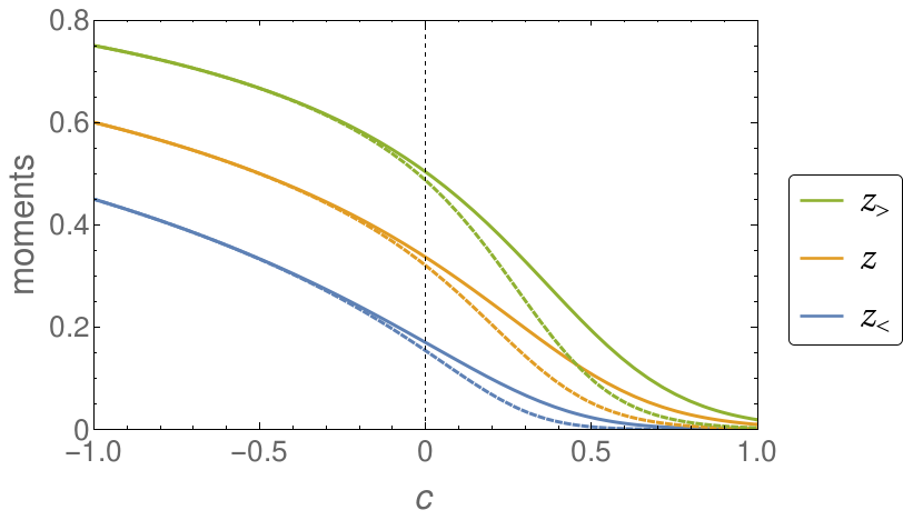
Figure 7: Values of $\left\langle{z^{2}/z_{R}^{2}}\right\rangle$ for left-handed fermion zero mode wavefunctions, plotted as functions of $c$, for (bottom to top) $z_{<}$, $z$, and $z_{>}$. Solid lines: $a$ = 0; Dashed lines: $a$ = 5.

Appendix D Construction of the $W$, $Z$, and $t$ propagators

Using the formalism of Appendices A and C, it is almost automatic to construct the gauge boson and top quark propagators. We present the essential formulae here.

D.1 $W$ propagator

The 5D $W$ boson is a mixture of the three fields $A_{m}^{aL},A_{m}^{aR},A_{m}^{a5}$, $a=1,2$, with boundary conditions shown in (9). The 5D propagator for these fields is given by (135). In this equation, ${\bf A}^{AB}$ is a $3\times 3$ matrix given by

$${\bf A}={\bf C}^{-1}{\bf D}\ ,$$ (212)

with

$${\bf C}=\pmatrix{{(1+c)\over 2}G_{W--}&{(1-c)\over 2}G_{W--}&-{s\over\sqrt{2}}G_{W-+}\cr{(1-c)\over 2}G_{+-}&{(1+c)\over 2}G_{+-}&{s\over\sqrt{2}}G_{++}\cr{s\over\sqrt{2}}G_{+-}&-{s\over\sqrt{2}}G_{+-}&c\ G_{++}\cr}$$ (213)

and

$${\bf D}=\pmatrix{-{(1+c)\over 2}G_{W-+}&-{(1-c)\over 2}G_{W-+}&-{s\over\sqrt{2}}G_{W--}\cr-{(1-c)\over 2}G_{++}&-{(1+c)\over 2}G_{++}&{s\over\sqrt{2}}G_{+-}\cr-{s\over\sqrt{2}}G_{++}&{s\over\sqrt{2}}G_{++}&c\ G_{+-}\cr}\ ,$$ (214)

where

$$G_{W--} = G_{--}+a_{W}pz_{0}G_{+-}$$

$$G_{W-+} = G_{-+}+a_{W}pz_{0}G_{++}\ .$$ (215)

Below, we will also need a similar modification for the $U(1)$ gauge field,

$$G_{B--} = G_{--}+a_{B}pz_{0}G_{+-}$$

$$G_{B-+} = G_{-+}+a_{B}pz_{0}G_{++}\ .$$ (216)

The mass eigenvalues in this sector and the contribution to the Coleman-Weinberg potential are controlled by the determinant of ${\bf C}$, which has the form,

$$\det{\bf C}=G_{+-}\biggl{[}G_{++}G_{W--}-{s^{2}\over 2p^{2}z_{0}z_{R}}\biggr{]}\ .$$ (217)

For our discussion of precision electroweak constraints, we will need the expansion of ${\bf A}$ including terms of order $s^{0}$ for the leading term in $p$ in each matrix element as $p\to 0$. It will suffice to ignore terms of order $z_{0}^{2}/z_{R}^{2}$. Then

$${\bf A}=-{2pz_{R}\over s^{2}}\pmatrix{1/2&{s^{2}/8}&{-s/\sqrt{2}pz_{R}}\cr{s^{2}/8}&s^{2}/4&0\cr{-s/\sqrt{2}pz_{R}}&0&(\log z_{R}/z_{0}+a_{W})\cr}\ .$$ (218)

From the definition (135), A must be symmetric. This is not obvious from (212), but it is true, and this is reflected in (218). The general proof of the Hermitian nature of A is given in Appendix E.

Now we find

$$\left\langle{A_{m}^{1L}(z)A_{n}^{1L}(z^{\prime})}\right\rangle \to \eta_{mn}kz_{R}^{2}\,p^{2}zz^{\prime}\biggl{[}-{1\over s^{2}}G_{+-}(z,z_{R})G_{+-}(z^{\prime},z_{R})$$ (219)

$$\hskip 86.72377pt+{1\over pz_{R}}G_{++}(z_{<},z_{R})G_{+-}(z_{>},z_{R})\biggr{]}$$

$$\to -\eta_{mn}{kz_{R}^{2}\over s^{2}}\biggl{[}1-{s^{2}\over 2}\Bigl{(}1-{z_{<}^{2}\over z_{R}^{2}}\Bigr{)}\biggr{]}$$

in the limit $p\to 0$, where $z_{<}$, $z_{>}$ are the smaller and larger of $z$, $z^{\prime}$. Similarly,

$$\left\langle{A_{m}^{1L}(z)A_{n}^{15}(z^{\prime})}\right\rangle \to \eta_{mn}kz_{R}^{2}\,p^{2}zz^{\prime}\biggl{[}{2s\over\sqrt{2}s^{2}pz_{R}}G_{+-}(z,z_{R})G_{++}(z^{\prime},z_{R})\biggr{]}$$ (220)

$$\to \eta_{mn}{kz_{R}^{2}\over s^{2}}\biggl{[}{s\over\sqrt{2}}\Bigl{(}1-{z^{\prime 2}\over z_{R}^{2}}\Bigr{)}\biggr{]}\ .$$

D.2 $Z$ propagator

The $Z$ propagator is derived in a similar way. In the basis $(A^{3L},B,Z^{\prime},A^{35})$ defined in (11) and (13), the matrix $U_{W}$ has the form

$$U_{W}=\pmatrix{(1+c)/2&s_{\beta}(1-c)/2&c_{\beta}(1-c)/2&-s/\sqrt{2}\cr s_{\beta}(1-c)/2&c_{\beta}^{2}+s_{\beta}^{2}(1+c)/2&-c_{\beta}s_{\beta}(1-c)/2&s_{\beta}s/\sqrt{2}\cr c_{\beta}(1-c)/2&-c_{\beta}s_{\beta}(1-c)/2&s_{\beta}^{2}+c_{\beta}^{2}(1+c)/2&c_{\beta}s/\sqrt{2}\cr s/\sqrt{2}&-s_{\beta}s/\sqrt{2}&-c_{\beta}s/\sqrt{2}&c}\ .$$ (221)

Then the C and D matrices are

$${\bf C}=\pmatrix{{(1+c)\over 2}G_{W--}&s_{\beta}{(1-c)\over 2}G_{W--}&c_{\beta}{(1-c)\over 2}G_{W--}&-{s\over\sqrt{2}}G_{W-+}\cr s_{\beta}{(1-c)\over 2}G_{B--}&(c_{\beta}^{2}+s_{\beta}^{2}{(1+c)\over 2})G_{B--}&-c_{\beta}s_{\beta}{(1-c)\over 2}G_{B--}&s_{\beta}{s\over\sqrt{2}}G_{B-+}\cr c_{\beta}{(1-c)\over 2}G_{+-}&-c_{\beta}s_{\beta}{(1-c)\over 2}G_{+-}&(s_{\beta}^{2}+c_{\beta}^{2}{(1+c)\over 2})G_{+-}&c_{\beta}{s\over\sqrt{2}}G_{++}\cr{s\over\sqrt{2}}G_{+-}&-s_{\beta}{s\over\sqrt{2}}G_{+-}&-c_{\beta}{s\over\sqrt{2}}G_{+-}&c\ G_{++}\cr}$$ (222)

and

$${\bf D}=\pmatrix{-{(1+c)\over 2}G_{W-+}&-s_{\beta}{(1-c)\over 2}G_{W-+}&-c_{\beta}{(1-c)\over 2}G_{W-+}&-{s\over\sqrt{2}}G_{W--}\cr-s_{\beta}{(1-c)\over 2}G_{B-+}&-(c_{\beta}^{2}+s_{\beta}^{2}{(1+c)\over 2})G_{B-+}&c_{\beta}s_{\beta}{(1-c)\over 2}G_{B-+}&s_{\beta}{s\over\sqrt{2}}G_{B--}\cr-c_{\beta}{(1-c)\over 2}G_{++}&c_{\beta}s_{\beta}{(1-c)\over 2}G_{++}&-(s_{\beta}^{2}+c_{\beta}^{2}{(1+c)\over 2})G_{++}&c_{\beta}{s\over\sqrt{2}}G_{+-}\cr-{s\over\sqrt{2}}G_{++}&s_{\beta}{s\over\sqrt{2}}G_{++}&c_{\beta}{s\over\sqrt{2}}G_{++}&c\ G_{+-}\cr}$$ (223)

The mass eigenvalues in this sector and the contribution to the Coleman-Weinberg potential are controlled by the determinant of ${\bf C}$. This is given by

$$\det{\bf C}=G_{+-}\biggl{[}G_{++}G_{W--}G_{B--}-{s^{2}\over 2p^{2}z_{0}z_{R}}(G_{B--}+s_{\beta}^{2}G_{W--})\biggr{]}\ .$$ (224)

D.3 $t$ propagator

The 5D $t$ quark is a mixture of the three fields $t_{L}$, $\chi_{b}$, $t_{R}$ in (22). The 5D propagator for these fields is given by (141). In the basis $(t_{L},\chi_{b},t_{R})$ used in (156), the ${\bf C}$ and ${\bf D}$ matrices take the form

$${\bf C}=\pmatrix{{(1+c)\over 2}G_{t--}&{(1-c)\over 2}G_{t--}&-{s\over\sqrt{2}}G_{t-+}\cr{(1-c)\over 2}G_{+-}&{(1+c)\over 2}G_{+-}&{s\over\sqrt{2}}G_{++}\cr{s\over\sqrt{2}}G_{+-}&-{s\over\sqrt{2}}G_{+-}&c\ G_{++}\cr}\ ,$$ (225)

and

$${\bf D}=\pmatrix{-{(1+c)\over 2}G_{t-+}&-{(1-c)\over 2}G_{t-+}&-{s\over\sqrt{2}}G_{t--}\cr-{(1-c)\over 2}G_{++}&-{(1+c)\over 2}G_{++}&{s\over\sqrt{2}}G_{+-}\cr-{s\over\sqrt{2}}G_{++}&{s\over\sqrt{2}}G_{++}&c\ G_{+-}\cr}\ ,$$ (226)

where

$$G_{t-\pm}=G_{-\pm}+a_{t}pz_{0}G_{+\pm}\ .$$ (227)

The mass eigenvalues in this sector and the contribution to the Coleman-Weinberg potential are controlled by the determinant of ${\bf C}$, which has the form,

$$\det{\bf C}=G_{+-}\biggl{[}G_{++}G_{t--}-{s^{2}\over 2p^{2}z_{0}z_{R}}\biggr{]}\ .$$ (228)

Appendix E Relation of the UV and IR gauges

In Section 4.5, we claimed that Green’s functions in the UV and IR gauges are related by the formula

$$(U_{W}^{\dagger})^{AC}\left\langle{A^{C}_{m}(z)A^{B}_{n}(z^{\prime})}\right\rangle_{IR}=\left\langle{A^{A}_{m}(z)A^{C}_{n}(z^{\prime})}\right\rangle_{UV}(U_{W}^{\dagger})^{CB}\ .$$ (229)

In this section, we prove this relation from the representations for the UV and IR gauge Green’s functions given in Appendix A. The idea of the proof is to use the identity (129) to relate $G_{ab}(z,z_{0})$ and $G_{ab}(z,z_{R})$. For definiteness, we consider the representations of the Green’s functions of the 4d components of a spin 1 field given in (135) and (137). It will be clear from the derivation that the result for all other RS Green’s functions can be carried out with the same logic.

We need to be very explicit about the boundary conditions on the various fields. We assign the field with gauge index $A$ the boundary conditions $a_{UV}=\pm$ and $a_{IR}=\pm$ in the UV and IR, respectively.

It suffices to consider the case $z>z^{\prime}$. In this case, the Green’s function on the right-hand side of (229) takes the form

$$\left\langle{A^{A}_{m}(z)A^{B}_{n}(z^{\prime})}\right\rangle_{UV} = \eta_{mn}kpz_{R}zz^{\prime}\biggl{[}G_{+,-a_{IR}}(z,z_{R}){\bf A}_{UV}^{AB}G_{+,-b_{IR}}(z^{\prime},z_{R})$$ (230)

$$\hskip 28.90755pt-G_{+,-a_{IR}}(z,z_{R})\delta^{AB}\tilde{G}_{+,-b_{IR}}(z^{\prime},z_{R})\biggr{]}\ .$$

From (136), the $\tilde{G}$ functions are given by

$$\tilde{G}_{c,-b_{IR}}=(-b_{IR})G_{c,+b_{IR}}\ .$$ (231)

In the second line of (230), we can put $a_{IR}=b_{IR}$.

In the UV gauge, the matrix ${\bf A}$ is computed as

$${\bf A}_{UV}={\bf C}^{-1}_{UV}{\bf D}_{UV}\ ,$$ (232)

The matrix elements of ${\bf C}$ and ${\bf D}$ are

$${\bf C}^{AB}_{UV} = U^{AB}G_{-a_{UV},-b_{IR}}(z_{0},z_{R})$$

$${\bf D}^{AB}_{UV} = U^{AB}\,(-b_{IR})\,G_{-a_{UV},+b_{IR}}(z_{0},z_{R})\ .$$ (233)

The formula (230) then factorizes as

$$\left\langle{A^{A}_{m}(z)A^{B}_{n}(z^{\prime})}\right\rangle_{UV} = \eta_{mn}kpz_{R}zz^{\prime}\biggl{[}G_{+,-a_{IR}}(z,z_{R}){\bf C}^{-1}_{UV}{}^{AC}$$

$$\hskip-28.90755pt\cdot\biggl{\{}{\bf D}_{UV}^{CB}G_{+,-b_{IR}}(z^{\prime},z_{R})-{\bf C}_{UV}^{CB}(-b_{IR})G_{+,+b_{IR}}(z^{\prime},z_{R})\biggr{\}}\biggr{]}$$

The term in braces is

$$\biggl{\{}G_{+,-b_{IR}}(z^{\prime},z_{R})(-b_{IR})G_{-c_{UV},+b_{IR}}(z_{0},z_{R})$$

$$\hskip 36.135pt-\ G_{+,+b_{IR}}(z^{\prime},z_{R})(-b_{IR})G_{-c_{UV},-b_{IR}}(z_{0},z_{R})\biggr{\}}U^{CB}$$

$$=\biggl{\{}G_{+,+}(z^{\prime},z_{R})G_{-c_{UV},-}(z_{0},z_{R})-G_{+,-}(z^{\prime},z_{R})G_{-c_{UV},+}(z_{0},z_{R})\biggr{\}}U^{CB}$$

$$={1\over pz_{R}}G_{+,-c_{UV}}(z,z_{0})U^{CB}\ ,$$ (235)

where, in the last line, we have used (129).

The UV gauge Green’s function then reassembles into

$$\left\langle{A^{A}_{m}(z)A^{B}_{n}(z^{\prime})}\right\rangle_{UV}=\eta_{mn}kzz^{\prime}\big{[}G_{+,-a_{IR}}(z,z_{R}){\bf C}^{-1}_{UV}{}^{AC}G_{+,-c_{UV}}(z^{\prime},z_{0})\big{]}U^{CB}\ .$$ (236)

The IR gauge Green’s function can be rearranged in a similar way.

$$\left\langle{A^{A}_{m}(z)A^{B}_{n}(z^{\prime})}\right\rangle_{IR} = -\eta_{mn}kpz_{0}zz^{\prime}\biggl{[}G_{+,-a_{UV}}(z,z_{0}){\bf A}_{IR}^{AB}G_{+,-b_{UV}}(z^{\prime},z_{0})$$ (237)

$$\hskip 28.90755pt-\tilde{G}_{+,-a_{UV}}(z,z_{0})\delta^{AB}G_{+,-b_{UV}}(z^{\prime},z_{0})\biggr{]}\ .$$

The $\tilde{G}$ functions are given by

$$\tilde{G}_{c,-a_{UV}}=(-a_{UV})G_{c,+a_{UV}}\ .$$ (238)

In the IR gauge, the matrix ${\bf A}$ is computed as

$${\bf A}_{IR}={\bf D}_{IR}{\bf C}^{-1}_{IR}\ ,$$ (239)

The matrix elements of ${\bf C}$ and ${\bf D}$ are

$${\bf C}^{AB}_{IR} = U^{AB}G_{-b_{IR},-a_{UV}}(z_{R},z_{0})$$

$${\bf D}^{AB}_{IR} = U^{AB}\,(-a_{UV})\,G_{-b_{IR},+a_{UV}}(z_{R},z_{0})\ .$$ (240)

The formula (237) then factorizes as

$$\left\langle{A^{A}_{m}(z)A^{B}_{n}(z^{\prime})}\right\rangle_{IR} = -\eta_{mn}kpz_{0}zz^{\prime}$$ (241)

$$\cdot\biggl{[}\biggl{\{}G_{+,-a_{UV}}(z,z_{0}){\bf D}^{AC}_{IR}-G_{+,+a_{UV}}(z,z_{0})(-a_{UV}){\bf C}_{IR}^{AC}\biggr{\}}$$

$$\hskip 43.36243pt\cdot({\bf C}^{-1}_{IR})^{CB}G_{+,-b_{UV}}(z^{\prime},z_{0})\biggr{]}\ .$$

The term in braces is

$$U^{AC}\biggl{\{}G_{+,-a_{UV}}(z,z_{0})(-a_{UV})G_{-c_{IR},+a_{UV}}(z_{R},z_{0})$$

$$\hskip 36.135pt-\ G_{+,+a_{UV}}(z,z_{0})(-a_{UV})G_{-c_{IR},-a_{UV}}(z_{R},z_{0})\biggr{\}}$$

$$=U^{AC}\biggl{\{}G_{+,+}(z,z_{0})G_{-c_{IR},-}(z_{R},z_{0})-G_{+,-}(z,z_{0})G_{-c_{IR},+}(z_{R},z_{0})\biggr{\}}$$

$$=U^{AC}{1\over pz_{0}}G_{+,-c_{IR}}(z,z_{R})\ ,$$ (242)

and again, in the last line, we have used (129).

The IR gauge Green’s function then reassembles into

$$\left\langle{A^{A}_{m}(z)A^{B}_{n}(z^{\prime})}\right\rangle_{IR}=-U^{AC}\eta_{mn}kzz^{\prime}\big{[}G_{+,-c_{IR}}(z,z_{R}){\bf C}^{-1}_{IR}{}^{CB}G_{+,-b_{UV}}(z^{\prime},z_{0})\big{]}\ .$$ (243)

To compare (236) and (243), note that (128) implies, using the explicit formulae above,

$$C_{IR}=-C_{UV}\ .$$ (244)

Then (236) and (243) have the same form, except that, in the latter, the matrix $U$ is moved to the right. This proves (229).

Notice that, in this calculation, the first index $+$ on the $G$ functions for the $A$ fields, the IR boundary condition of $A^{A}_{m}$, and the UV boundary condition of $A^{B}_{n}$ play no role in the cancellation. The parallel calculation for $z<z^{\prime}$ depends on the IR boundary condition of $A^{B}_{n}$ and the UV boundary condition of $A_{m}^{A}$ and also goes through for any values of these. The $G$ functions in the cancellation are linked by $U$ matrices and therefore have the same value of $c$. Thus, the same argument goes through for any Green’s function of RS fields.

Using the same method, one can prove the identity

$${\bf D}{\bf C}^{\dagger}-{\bf C}{\bf D}^{\dagger}=0$$ (245)

for both the UV and IR forms of these matrices. After the use of the identity (129), one finds that the $G$ functions combine into

$$G_{a,a}(z_{R},z_{R})\quad\mbox{or}\quad G_{a,a}(z_{0},z_{0})\ .$$ (246)

These expressions are zero by (128). This identity implies the Hermitian property for the ${\bf A}$ matrices discussed at the end of Appendix A.

Appendix F Small $s$ expansion of the Coleman-Weinberg potentials

In this appendix, we discuss the expansion of the Coleman-Weinberg potentials (56), (LABEL:VZ), (69), and (70) for small values of $s$. Here we generalize the discussion on the Coleman-Weinberg potentials in [21] and include the effect of the boundary kinetic terms.

Analogously to the definition of $G_{\alpha\beta}$ in (7), we define the Green’s functions $G_{E\alpha\beta}$ in Euclidean momentum:

$$G_{E\alpha\beta}(z_{1},z_{2})=K_{\alpha}(p_{E}z_{1})I_{\beta}(p_{E}z_{2})-(-1)^{\delta}I_{\alpha}(p_{E}z_{1})K_{\beta}(p_{E}z_{2})\ ,$$ (247)

where $(-1)^{\delta}=1$ for $\alpha=\beta$ and $-1$ for $\alpha\neq\beta$. The Green’s functions are positive definite. For large $p_{E}$, we have

$$G_{E\alpha\beta}(z_{0},z_{R})\sim e^{p_{E}(z_{R}-z_{0})}\ .$$ (248)

First we consider the potential $V_{T}$ in (70). Note that

$$s_{2}^{2}(2-s_{2}^{2})={1\over 2}s^{2}+{1\over 16}s^{4}+{\cal O}(s^{6})\ .$$ (249)

Then the integrand can be expanded about $s^{2}=0$ under the integral sign. After the expansion, we get

$$V_{T}(h)={N_{T}k_{R}^{4}\over 4\pi^{2}}\left[A_{T}(c_{T})\left({1\over 2}s^{2}+{1\over 16}s^{4}\right)+{1\over 8}B_{T}(c_{T})s^{4}+{\cal O}(s^{6})\right]\ ,$$ (250)

where $N_{T}$ is the number of QCD colors of $\Psi_{T}$. Whether $N_{T}=3$ or 1 is a model-building choice. The coefficients $A_{T}$ and $B_{T}$ are given by

$$A_{T}(c) = \int_{0}^{\infty}dp_{E}\,p_{E}^{3}\ {z_{R}^{4}\over p_{E}^{2}z_{0}z_{R}G_{E-+}G_{E+-}}$$

$$B_{T}(c) = \int_{0}^{\infty}dp_{E}\,p_{E}^{3}\ {z_{R}^{4}\over(p_{E}^{2}z_{0}z_{R}G_{E-+}G_{E+-})^{2}}\ ,$$ (251)

and both are positive definite for all values of $c$. For $p_{E}\to 0$,

$$G_{E-+}G_{E+-}={1\over p_{E}^{2}z_{0}z_{R}}(1+{\cal O}(p_{E}^{2}))\ ,$$ (252)

and therefore together with (248), the integrals are convergent. Rescaling $p\rightarrow pz_{R}$ in (251) shows that $A_{T}$ and $B_{T}$ depend only on the ratio $z_{R}/z_{0}$, not on $z_{0}$ or $z_{R}$ individually. For the representative case $z_{R}/z_{0}=100$, the values of these coefficients at $c=0$ are

$$A_{T}(0)=1.4078,\qquad B_{T}(0)=0.21694\ ,$$ (253)

and they decrease as $c$ increases. Note that $B_{T}$ is much smaller than $A_{T}$.

We can similarly proceed for the top quark contribution $V_{t}$ in (69), but for this case more care is necessary due to IR divergence of the integrand. Following the prescription given in [21], we get

$$V_{t}(h)={3k_{R}^{4}\over 4\pi^{2}}\left[-{1\over 2}A_{t}(c_{t})s^{2}+{1\over 8}B_{t}(c_{t})s^{4}+{1\over 8}C_{t}(c_{t})s^{4}\log{1\over s^{2}/2}+{\cal O}(s^{6})\right]$$ (254)

where we define

$$A_{t}(c) = \int_{0}^{\infty}dp_{E}\,p_{E}^{3}\ {z_{R}^{4}\over p_{E}^{2}{\bf G}_{t}(p_{E})}$$

$$B_{t}(c) = z_{R}^{4}\biggl{[}{1\over{\bf G}_{t}(0)^{2}}[{1\over 4}-{\gamma\over 2}]+\int_{0}^{\infty}{dp_{E}\over p_{E}}\ \bigl{\{}{1\over{\bf G}_{t}(p_{E})^{2}}-{1\over{\bf G}_{t}(0)^{2}}e^{-{\bf G}_{t}(0)p_{E}^{2}}\bigr{\}}\biggr{]}$$

$$C_{t}(c) = {z_{R}^{4}\over 2{\bf G}_{t}(0)^{2}}$$ (255)

and

$${\bf G}_{t}(p_{E})=z_{0}z_{R}G_{E++}(G_{E--}+a_{t}p_{E}z_{0}G_{E+-})\ .$$ (256)

For $z_{R}/z_{0}=100$ and $a_{t}=0$, the values of these coefficients at $c=0$ are

$$A_{t}(0)=1.8771,\qquad B_{t}(0)=0.19585,\qquad C_{t}(0)=0.52051\ ,$$ (257)

and they decrease as $c$ increases. Here we can also see that a large boundary kinetic term $a_{t}$ will suppress the potential. Note that $B_{t}$ and $C_{t}$ are much smaller than $A_{t}$.

Finally, for $V_{W}$ (56) and $V_{Z}$ (LABEL:VZ), we have

$$V_{W}(h) = {3k_{R}^{4}\over 8\pi^{2}}\left[{1\over 2}A_{W}s^{2}-{1\over 8}B_{W}s^{4}-{1\over 8}C_{W}s^{4}\log{1\over s^{2}/2}+{\cal O}(s^{6})\right]$$

$$V_{Z}(h) = {3k_{R}^{4}\over 16\pi^{2}}\left[{1\over 2}A_{Z}s^{2}-{1\over 8}B_{Z}s^{4}-{1\over 8}C_{Z}s^{4}\log{1\over s^{2}/2}+{\cal O}(s^{6})\right]\ ,$$ (258)

where the coefficients can be obtained from (255) by replacing ${\bf G}_{t}$ with

$${\bf G}_{W}(p_{E}) = z_{0}z_{R}G_{E++}(G_{E--}+a_{W}p_{E}z_{0}G_{E+-})$$

$${\bf G}_{Z}(p_{E}) = {z_{0}z_{R}G_{E++}(G_{E--}+a_{B}p_{E}z_{0}G_{E+-})\over(G_{E--}+a_{B}p_{E}z_{0}G_{E+-})+s_{\beta}^{2}(G_{E--}+a_{W}p_{E}z_{0}G_{E+-})}$$ (259)

where $c=1/2$. It is instructive to note that because of the factor of 3 from $SU(3)_{C}$ color, the fermion contribution to the Higgs potential is usually larger than that of gauge bosons. In realisitic models, the gauge boson boundary kinetic term further suppresses $V_{W}$ and $V_{Z}$ and therefore makes them almost negligible compared to the potential by fermions, especially when $c_{t}$ and $c_{T}$ are small.

Summing up, we get the expansion of the full Higgs potential (72)

$$V(h)={k_{R}^{4}\over 8\pi^{2}}\left[-As^{2}+{1\over 2}Bs^{4}+{1\over 2}Cs^{4}\log{1\over s^{2}}+{\cal O}(s^{6})\right]\ ,$$ (260)

where

$$A = 3A_{t}(c_{t})-N_{T}A_{T}(c_{T})-{3\over 2}A_{W}-{3\over 4}A_{Z}$$

$$B = {3\over 2}(B_{t}(c_{t})+C_{t}(c_{t})\log 2)+{N_{T}\over 4}A_{T}(c_{T})+{N_{T}\over 2}B_{T}(c_{T})$$

$$\hskip 21.68121pt-{3\over 4}(B_{W}+C_{W}\log 2)-{3\over 8}(B_{Z}+C_{Z}\log 2)$$

$$C = {3\over 2}C_{t}(c_{t})-{3\over 4}C_{W}-{3\over 8}C_{Z}\ .$$ (261)

We can make further approximations on the potential, using that $B_{T,t}$ and $C_{T,t}$ are much smaller than $A_{T,t}$. Furthermore, the gauge boson terms are suppressed if it includes large UV boundary kinetic terms, which indeed is the case for our model. Then, we have

$$A \sim 3A_{t}(c_{t})-N_{T}A_{T}(c_{T})$$

$$B \sim {N_{T}\over 4}A_{T}(c_{T})$$

$$C \sim 0\ .$$ (262)

If we tune $c_{t}$ and $c_{T}$ so that $A\sim 0$, we can realize $v\ll f$. In this case, we have $B\sim{3\over 4}A_{t}(c_{t})$. With this crude approximation, we can get a simple relationship between the Higgs mass to the top quark mass, which is independent on $c_{t}$ and $a_{t}$.

It should be noted that $\frac{3}{4}A_{T}$ in $B$ gives a large contribution to the Higgs quartic potential. This term appears as we embed $\Psi_{T}$ in 5 of $SO(5)$, as in (22). With the 4 representaion in (21), we do not have such term and it makes the parameter space of the 4 model more constrained than that of the 5.

Appendix G Coefficients in the fermion loop correction to $T$ parameter

In this Appendix, we calculate the coefficients $A$, $B$, and $C$ needed in the calculation of the RS correction to the $T$ parameter from (107). For this, we need to compute the $LL$ components of the $t_{L}$ and $b_{L}$ propagators in Euclidean space, as indicated in (106). These coefficients depend on the arguments of the Green’s functions $z$ and $z^{\prime}$ as well as on the Euclidean momentum $p$ and $m_{t}$.

In (141), we showed that the fermion Green’s functions in the UV gauge are a sum of two terms, the first of which contains the matrix ${\bf A}={\bf C}^{-1}{\bf D}$ and the second of which contains the unit matrix and is independent of boundary mixing. This latter term is identical for $t_{L}$ and $b_{L}$, since both have $+$ boundary conditions on the IR brane. So we will ignore this second term, since it does not contribute to the difference of the propagators.

We now need to compute the ${\bf A}$ coefficients for $t_{L}$ and $b_{L}$. For $b_{L}$, an unmixed fermion with $++$ boundary conditions, we did this calculation already in (198) and found

$${\bf A}=-{G_{t-+}\over G_{t--}}\ ,$$ (263)

where $G_{t-\pm}$ are defined in (227). The same result carries over to Euclidean space, with $G$ replaced by $G_{E}$. In the analysis below, we will abbreviate $G_{E\alpha\beta}(z_{0},z_{R})$ by $G_{E\alpha\beta}$.

It will be useful to adopt a compact notation for the expansions of the $G$ functions. We will write

$$G_{E++}(z,z_{R};p)=G_{E++}(z,z_{R};p=0)\bigl{[}1+(pz_{R})^{2}{\cal Z}_{++}(z)+\cdots\bigr{]}\ ,$$ (264)

and similarly for the other $G_{E}$ functions, putting the appropriate subscript on the ${\cal Z}$ coefficient. Using this notation, it follows from (263) and the Euclidean version of (141) that

$$C={\cal Z}_{t-+}(z_{0})-{\cal Z}_{t--}(z_{0})+{\cal Z}_{+-}(z)+{\cal Z}_{+-}(z^{\prime})\ .$$ (265)

To evaluate the $t_{L}$ propagator, we need to compute the $3\times 3$ matrix ${\bf A}$ for this case. We find

$${\bf A}^{11}=-G_{E++}\left({1\over p^{2}z_{0}z_{R}}+G_{E++}G_{Et--}+{\cal O}(s^{4})\right)/\det{\bf C}\ .$$ (266)

Using the Euclidean space form of the Wronskian identity

$$G_{E++}(z_{1},z_{2})G_{E--}(z_{1},z_{2})-G_{E+-}(z_{1},z_{2})G_{E-+}(z_{1},z_{2})=-{1\over p^{2}z_{1}z_{2}}\ ,$$ (267)

this becomes

$${\bf A}^{11}=-G_{E++}G_{E+-}G_{Et-+}/\det{\bf C}\ .$$ (268)

Further,

$${1\over\det{\bf C}}={1\over G_{E++}G_{E+-}G_{Et--}}{p^{2}\over p^{2}+m_{t}^{2}}\left(1+(m_{t}z_{R})^{2}({\cal Z}_{++}+{\cal Z}_{t--})\right)\ ,$$ (269)

so

$${\bf A}_{11}=-{G_{Et-+}\over G_{Et--}}{p^{2}\over p^{2}+m_{t}^{2}}\left(1+(m_{t}z_{R})^{2}({\cal Z}_{++}+{\cal Z}_{t--})\right)\ ,$$ (270)

in parallel with (263). Similarly,

$${\bf A}_{13}={\bf A}_{31}={s/\sqrt{2}\over p^{2}z_{0}z_{R}G_{E++}G_{Et--}}{p^{2}\over p^{2}+m_{t}^{2}}\ ,$$ (271)

up to ${\cal O}(s^{2})$.

We now transform to the IR gauge using (71). Up to ${\cal O}(s^{2})$, the relevant terms are

$$\left\langle{(t_{L})_{L}(t_{L})_{L}^{\dagger}}\right\rangle_{IR,11} = (1-{s^{2}\over 2})\left\langle{(t_{L})_{L}(t_{L})_{L}^{\dagger}}\right\rangle_{UV,11}$$ (272)

$$\hskip-7.22743pt+(-{s\over\sqrt{2}})\left\langle{(t_{L})_{L}(t_{L})_{L}^{\dagger}}\right\rangle_{UV,13}+(-{s\over\sqrt{2}})\left\langle{(t_{L})_{L}(t_{L})_{L}^{\dagger}}\right\rangle_{UV,31}$$

We must now expand this expression and set the result into the form (108). The terms explicitly proportional to $s^{2}$ are contributions to the $A$ coefficient, since, from (68)

$$m_{t}^{2}z_{R}^{2}=s^{2}{2c_{t}+1\over 2L_{t}}\biggl{(}{z_{0}\over z_{R}}\biggr{)}^{c_{t}-1/2}\ .$$ (273)

We then find for the $A$ coefficient

$$A = {L_{t}\over(2c_{t}+1)}\biggl{(}{z_{R}\over z_{0}}\biggr{)}^{c_{t}-1/2}\left\{-1+(2c_{t}+1)\left[({z\over z_{R}})^{c_{t}+1/2}R(z)+({z^{\prime}\over z_{R}})^{c_{t}+1/2}R(z^{\prime})\right]\right\}$$ (274)

$$\hskip 21.68121pt+{\cal Z}_{++}(z_{0})+{\cal Z}_{t--}(z_{0})\ ,$$

where $R(z)=G_{E++}(z,z_{R};p=0)$. The $B$ coefficient is

$$B=C={\cal Z}_{t-+}(z_{0})-{\cal Z}_{t--}(z_{0})+{\cal Z}_{+-}(z)+{\cal Z}_{+-}(z^{\prime})\ .$$ (275)

To evaluate the expressions for $A$, $B$, and $C$, we need the expansions

$$R(z) = {1\over 2c+1}\biggl{[}\bigl{(}{z_{R}\over z}\bigr{)}^{c+1/2}-({z\over z_{R}}\bigr{)}^{c+1/2}\biggr{]}$$

$${\cal Z}_{++}(z_{0}) = {1\over 2(2c+3)}$$

$${\cal Z}_{t--}(z_{0}) = {1\over 2(2c+1)L_{t}}\biggl{(}{1\over(2c-3)}\biggl{\{}\bigl{[}({z_{R}\over z_{0}})^{c-1/2}+({z_{0}\over z_{R}})^{c-1/2}\bigr{]}$$

$$\hskip 14.45377pt-{2\over 2c-1}\bigl{[}({z_{R}\over z_{0}})^{c-1/2}-({z_{0}\over z_{R}})^{c-1/2}\bigr{]}\biggr{\}}+a_{t}({z_{R}\over z_{0}})^{c-1/2}\biggr{)}$$

$${\cal Z}_{t-+}(z_{0}) = -{1\over 2(2c+1)}\biggl{[}1+{2\over 2c-1}\bigl{(}1-({z_{R}\over z_{0}})^{2c-1}\bigr{)}\biggr{]}+{a_{t}\over 2c+1}({z_{R}\over z_{0}})^{2c-1}$$

$${\cal Z}_{+-}(z) = {1\over 2(2c+1)}\biggl{(}1-{z^{2}\over z_{R}^{2}}\bigl{[}1+{2\over 2c-1}(1-({z\over z_{R}})^{2c-1})\bigr{]}\biggr{)}\ .$$ (276)

We have made the above formulae somewhat simpler by ignoring factors of $(z_{0}/z_{R})$ and $(z_{0}/z_{R})^{c+1/2}$ (but not $(z_{0}/z_{R})^{c-1/2}$) for the relevant values $c>0.3$. Also note that there is an identity between the expressions above,

$${z_{0}\over z_{R}}R(z_{0})L_{t}={\cal Z}_{+-}(z_{0})+{\cal Z}_{t-+}(z_{0})$$ (277)

which follows from the Wronskian identity (267).

Using these formulae, our estimate of the correction to $T$ can be written as

$$T \approx {3m_{t}^{2}\over 16\pi s_{w}^{2}c_{w}^{2}m_{Z}^{2}}\Biggl{\{}2(m_{t}z_{R})^{2}\biggl{[}\left\langle{{\cal Z}_{+-}(z)+{\cal Z}_{+-}(z^{\prime})}\right\rangle-2{\cal Z}_{t--}(z_{0})-{\cal Z}_{++}(z_{0})-{\cal Z}_{+-}(z_{0})\biggr{]}$$ (278)

$$\hskip 72.26999pt+s^{2}\left\langle{({z\over z_{R}})^{1+2c_{t}}+({z^{\prime}\over z_{R}})^{1+2c_{t}}}\right\rangle\Biggr{\}}\cdot\log\left(\Lambda^{2}/m_{t}^{2}\right)\ .$$

In our discussion of parameters, we saw that $a_{t}$ has a large value, of order 10. Then it makes sense to extract the terms in (278) that are enhanced by a power of $a_{t}$. These come from the term with $s^{2}$, which is proportional to $L_{t}$ through (273). Keeping only this term, we find a much simpler expression, which is quoted in (112). However, the small values of the expectation values of $z$ and $z^{\prime}$ counterbalance the large value of $a_{t}$, so this parametrically large contributin is not actually dominant. The values of $T$ in Fig. 6 are evaluated with the full expression (278).

ACKNOWLEDGEMENTS

We are grateful to Christophe Grojean, Howard Haber, Hitoshi Murayama, Yael Shadmi, and the members of the SLAC Theory Group for informative discussions of the topics presented in this paper. This work was supported by the U.S. Department of Energy under contract DE–AC02–76SF00515. JY is supported by a Kwanjeong Graduate Fellowship.

References

- [1] M. Drees, R. Godbole, and P. Roy, Theory and Phenomenology of Sparticles (World Scientific Pres, 2005).
- [2] H. Baer and X. Tata, Weak Scale Supersymmetry. (Cambridge University Press, 2006).
- [3] C. F. Berger, J. S. Gainer, J. L. Hewett and T. G. Rizzo, JHEP 0902, 023 (2009); [arXiv:0812.0980 [hep-ph]]; M. Cahill-Rowley, J. L. Hewett, A. Ismail and T. G. Rizzo, arXiv:1307.8444 [hep-ph].
- [4] A. De Simone, O. Matsedonskyi, R. Rattazzi and A. Wulzer, JHEP 1304, 004 (2013) [arXiv:1211.5663 [hep-ph]].
- [5] B. Bellazzini, C. Csáki and J. Serra, Eur. Phys. J. C 74, 2766 (2014) [arXiv:1401.2457 [hep-ph]].
- [6] C. Csaki, C. Grojean and J. Terning, Rev. Mod. Phys. 88, 045001 (2016) [arXiv:1512.00468 [hep-ph]].
- [7] K. Agashe, R. Contino and A. Pomarol, Nucl. Phys. B 719, 165 (2005) [hep-ph/0412089].
- [8] M. Carena, E. Ponton, J. Santiago and C. E. M. Wagner, Nucl. Phys. B 759, 202 (2006) [hep-ph/0607106].
- [9] D. Croon, B. M. Dillon, S. J. Huber and V. Sanz, JHEP 1607, 072 (2016) [arXiv:1510.08482 [hep-ph]].
- [10] L. Randall and R. Sundrum, Phys. Rev. Lett. 83, 3370 (1999) [hep-ph/9905221].
- [11] N. Arkani-Hamed, M. Porrati and L. Randall, JHEP 0108, 017 (2001) [hep-th/0012148].
- [12] L. J. Hall, Y. Nomura and D. Tucker-Smith, Nucl. Phys. B 639, 307 (2002) [hep-ph/0107331].
- [13] M. Kubo, C. S. Lim and H. Yamashita, Mod. Phys. Lett. A 17, 2249 (2002) [hep-ph/0111327].
- [14] Y. Hosotani, Phys. Lett. B 126, 309 (1983).
- [15] D. J. Toms, Phys. Lett. B 126, 445 (1983).
- [16] R. Contino, Y. Nomura and A. Pomarol, Nucl. Phys. B 671, 148 (2003) [hep-ph/0306259].
- [17] C. S. Lim and N. Maru, Phys. Rev. D 75, 115011 (2007) [hep-ph/0703017]; Y. Adachi and N. Maru, Phys. Rev. D 98, 015022 (2018) [arXiv:1804.06012 [hep-ph]].
- [18] A. D. Medina, N. R. Shah and C. E. M. Wagner, Phys. Rev. D 76, 095010 (2007) [arXiv:0706.1281 [hep-ph]].
- [19] M. Carena, A. D. Medina, B. Panes, N. R. Shah and C. E. M. Wagner, Phys. Rev. D 77, 076003 (2008) [arXiv:0712.0095 [hep-ph]].
- [20] S. Casagrande, F. Goertz, U. Haisch, M. Neubert and T. Pfoh, JHEP 1009, 014 (2010) [arXiv:1005.4315 [hep-ph]].
- [21] J. Yoon and M. E. Peskin, Phys. Rev. D 96, 115030 (2017) [arXiv:1709.07909 [hep-ph]].
- [22] M. E. Peskin and T. Takeuchi, Phys. Rev. Lett. 65, 964 (1990), Phys. Rev. D 46, 381 (1992).
- [23] R. S. Chivukula, S. B. Selipsky and E. H. Simmons, Phys. Rev. Lett. 69, 575 (1992) [hep-ph/9204214]; R. S. Chivukula, E. H. Simmons and J. Terning, Phys. Lett. B 331, 383 (1994) [hep-ph/9404209].
- [24] J. Yoon and M. E. Peskin, arXiv:1811.07877 [hep-ph].
- [25] L. Randall and M. D. Schwartz, JHEP 0111, 003 (2001) [hep-th/0108114].
- [26] W. D. Goldberger and M. B. Wise, Phys. Rev. D 60, 107505 (1999) [hep-ph/9907218].
- [27] H. Davoudiasl, J. L. Hewett and T. G. Rizzo, Phys. Rev. Lett. 84, 2080 (2000) [hep-ph/9909255], Phys. Lett. B 473, 43 (2000) [hep-ph/9911262].
- [28] T. Gherghetta and A. Pomarol, Nucl. Phys. B 586, 141 (2000) [hep-ph/0003129], Nucl. Phys. B 602, 3 (2001) [hep-ph/0012378].
- [29] P. Sikivie, L. Susskind, M. B. Voloshin and V. I. Zakharov, Nucl. Phys. B 173, 189 (1980).
- [30] Y. Grossman and M. Neubert, Phys. Lett. B 474, 361 (2000) [hep-ph/9912408].
- [31] K. Agashe and R. Contino, Nucl. Phys. B 742, 59 (2006) [hep-ph/0510164].
- [32] K. Agashe, R. Contino, L. Da Rold and A. Pomarol, Phys. Lett. B 641, 62 (2006) [hep-ph/0605341].
- [33] R. Contino, L. Da Rold and A. Pomarol, Phys. Rev. D 75, 055014 (2007) [hep-ph/0612048].
- [34] D. Buttazzo, G. Degrassi, P. P. Giardino, G. F. Giudice, F. Sala, A. Salvio and A. Strumia, JHEP 1312, 089 (2013) [arXiv:1307.3536 [hep-ph]].
- [35] A. Falkowski, Phys. Rev. D 75, 025017 (2007) [hep-ph/0610336], arXiv:0710.4050 [hep-ph].
- [36] M. Aaboud et al. [ATLAS Collaboration], JHEP 1710, 182 (2017) [arXiv:1707.02424 [hep-ex]].
- [37] A. M. Sirunyan et al. [CMS Collaboration], JHEP 1806, 120 (2018) [arXiv:1803.06292 [hep-ex]].
- [38] M. Aaboud et al. [ATLAS Collaboration], [arXiv:1808.02343 [hep-ex]].
- [39] ATLAS Collaboration, ATLAS-CONF-2018-020.
- [40] Z. Chacko, H. S. Goh and R. Harnik, Phys. Rev. Lett. 96, 231802 (2006) [hep-ph/0506256]; G. Burdman, Z. Chacko, H. S. Goh and R. Harnik, JHEP 0702, 009 (2007) [hep-ph/0609152].
- [41] N. Craig, S. Knapen and P. Longhi, Phys. Rev. Lett. 114, no. 6, 061803 (2015) [arXiv:1410.6808 [hep-ph]].
- [42] M. E. Peskin and J. D. Wells, Phys. Rev. D 64, 093003 (2001) [hep-ph/0101342].
- [43] J. Erler and A. Frietas, in M. Tanabashi et al. [Particle Data Group], Phys. Rev. D 98, no. 3, 030001 (2018).
- [44] J. L. Hewett, F. J. Petriello and T. G. Rizzo, JHEP 0310, 062 (2003) [hep-ph/0211218].
- [45] M. C. Chen and S. Dawson, Phys. Rev. D 70, 015003 (2004) [hep-ph/0311032].
- [46] S. Schael et al. [ALEPH and DELPHI and L3 and OPAL and SLD Collaborations and LEP Electroweak Working Group and SLD Electroweak Group and SLD Heavy Flavour Group], Phys. Rept. 427, 257 (2006) [hep-ex/0509008].