Ultra-high energy cosmic rays from shocks in the lobes of powerful radio galaxies

Abstract

The origin of ultra-high energy cosmic rays (UHECRs) has been an open question for decades. Here, we use a combination of hydrodynamic simulations and general physical arguments to demonstrate that UHECRs can in principle be produced by diffusive shock acceleration (DSA) in shocks in the backflowing material of radio galaxy lobes. These shocks occur after the jet material has passed through the relativistic termination shock. Recently, several authors have demonstrated that highly relativistic shocks are not effective in accelerating UHECRs. The shocks in our proposed model have a range of non-relativistic or mildly relativistic shock velocities more conducive to UHECR acceleration, with shock sizes in the range $1-10$ kpc. Approximately 10% of the jet’s energy flux is focused through a shock in the backflow of $M>3$. Although the shock velocities can be low enough that acceleration to high energy via DSA is still efficient, they are also high enough for the Hillas energy to approach $10^{19-20}$ eV, particularly for heavier CR composition and in cases where fluid elements pass through multiple shocks. We discuss some of the more general considerations for acceleration of particles to ultra-high energy with reference to giant-lobed radio galaxies such as Centaurus A and Fornax A, a class of sources which may be responsible for the observed anisotropies from UHECR observatories.

1 Introduction

Ultra-high energy cosmic rays (UHECRs) are cosmic rays (CRs) that arrive at Earth with energies extending beyond $10^{20}$ eV. Although the acceleration of Galactic CRs with energies of about $100$ TeV in supernova remnants (SNRs) is well-established (Völk et al., 2005; Uchiyama et al., 2007; Bell, 2014), as yet, the origin of UHECRs is not known. They must be extragalactic, since their Larmor radius in a reasonable background magnetic field is larger than the Galactic scale height ($\sim 1$ kpc), but they must originate from within a few mean free paths for attenuation by the Greisen–Zatsepin–Kuzmin (GZK; Greisen, 1966; Zatsepin & Kuz’min, 1966) effect and photodisintegration (e.g. Stecker & Salamon, 1999). Both processes have a typical attenuation length of $\sim 50-100$Mpc (e.g. Alves Batista et al., 2016; Wykes et al., 2017). Furthermore, any complete production model must explain the observed anisotropies (Abu-Zayyad et al., 2013; Abbasi et al., 2014; Pierre Auger Collaboration et al., 2017, 2018) and the composition of CRs at high energies (Pierre Auger Collaboration, 2014; de Souza, 2017). Meeting all these requirements simultaneously is a challenge.

One of the best candidate mechanisms for accelerating CRs to high energy is diffusive shock acceleration (DSA; Axford et al., 1977; Krymskii, 1977; Blandford & Ostriker, 1978; Bell, 1978a, b), also known as first order Fermi acceleration. The characteristic maximum energy a CR can gain by this process is set by the Hillas energy (Hillas, 1984), given by

$$E_{H}=0.9~{}\mathrm{EeV}~{}Z\left(\frac{B}{\mu\mathrm{G}}\right)\left(\frac{v_{s}}{c}\right)\left(\frac{r}{\mathrm{kpc}}\right),$$ (1)

where $B$ is the magnetic field, $v_{s}$ is the shock velocity, $Z$ is the atomic number of the nucleus and $r$ is the characteristic size of the shock. While other mechanisms such as second-order Fermi acceleration (Fermi, 1949), shock drift acceleration (e.g. Armstrong et al., 1985; Burgess, 1987; Decker, 1988) and “one-shot” mechanisms (e.g. Litvinenko, 1996; Haswell et al., 1992; Caprioli, 2015) may also work, DSA is attractive since it naturally produces a power law similar to that observed and also probably accelerates the electrons in SNR and radio galaxies to high energy where radiation is clearly emitted near shock fronts (e.g. Laing, 1989; Koyama et al., 1995).

Given the dependence of the Hillas energy on shock size and speed, it is natural to turn to the largest systems we know of that show energetic outflows and strong shocks. In this sense, active galactic nuclei (AGN) and their associated outflows make for obvious UHECR candidate sources (e.g. Hillas, 1984; Norman et al., 1995; O’Sullivan et al., 2009; Hardcastle, 2010). AGN can launch dramatic jets from close to the black hole, which can then travel for hundreds of kpc into the surrounding medium, producing giant radio galaxies. Radio galaxies typically fall into one of two Fanaroff & Riley (1974) classes; class I sources (FRIs) are brightest at the centre and have fairly low power jets that entrain material, becoming disrupted relatively close to the nucleus, whereas class IIs (FRIIs) can proceed uninterrupted for long distances, showing bright ‘hotspots’ at the ends of the jets where they produce a termination shock.

Catalogues of AGN and radio galaxy positions can be correlated with the arrival directions from the Pierre Auger Observatory (PAO) and other UHECR detectors. Initial PAO results suggested an association with AGN (Pierre Auger Collaboration et al., 2007, 2008), but updated results were of lower significance (Abreu et al., 2010). However, more recently significant departures from isotropy have been observed (Pierre Auger Collaboration et al., 2017, 2018), with Pierre Auger Collaboration et al. (2018) finding significant correlations of 4 and 2.7$\sigma$ with starburst galaxies and AGN, respectively. However, as we showed in a recent Letter (Matthews et al., 2018), considering the most recent Fermi catalogues and accounting for magnetic deflection can increase the correlation with AGN, particularly if the local contribution to UHECRs is dominated by Fornax A and Centaurus A.

Despite the promise of radio galaxies as UHECR sources, relativistic shocks such as their termination shocks are actually rather poor accelerators of UHECRs (Lemoine & Pelletier, 2010; Kirk & Reville, 2010; Reville & Bell, 2014; Bell et al., 2018). In a recent paper, we showed that the maximum energy in an ultra-relativistic shock is well below the EeV range (Bell et al., 2018). We also applied similar arguments to the observed radio spectra in the hotspots of Cygnus A (Araudo et al., 2018) and other FRII sources (Araudo et al., 2015, 2016). These studies show that while magnetic field amplification to above $100\mu$G can occur, the maximum energy of the non-thermal electrons is rather low, on the order of a TeV. This maximum energy and associated synchrotron cutoff is set by the detailed plasma physics and ability to drive Larmor-scale turbulence at the shock, rather than synchrotron cooling, and thus this limit also applies to CR protons and nuclei; the limit can however be relaxed if there is pre-existing turbulent magnetic field on the right scale to scatter particles. Nonetheless, it seems that if radio galaxies are to accelerate UHECRs via DSA then a balance must be struck between allowing the Hillas energy to be high enough, and not inhibiting the self-regulating acceleration process. In other words, a “goldilocks” zone in which the shock parameters are “just right” for efficient DSA to high energy must exist. The motivation for this paper is to search for shocks in radio galaxies that meet these requirements (i.e. not the relativistic termination shock) and offer favourable conditions for CR acceleration to ultra-high energy.

The paper is structured as follows. We introduce our numerical method in section 2, before describing the simulation results in section 3. In section 4 we use some simple Bernoulli-like arguments to study the flow of plasma in the jet lobe and cocoon. In section 5, we use a combination of Lagrangian and Eulerian methods to calculate the shock properties in the simulation, which are then used to estimate the maximum CR energy in section 6. We discuss our results in section 7, with particular reference to radio galaxy luminosity functions, power requirements and results from UHECR observatories, before concluding in section 8. We adopt the convention of referring to a cocoon as all the shocked jet material that enshrouds the jet beam, and a lobe as the cocoon material close to the hotspot that is typically observed in radio. We refer to kinetic powers, radiative luminosities and pressures with the symbols $Q$, $L$ and $P$, respectively.

2 Numerical Method

We use the freely available Godunov-type Eulerian code Pluto (Mignone et al., 2007) to solve the equations of relativistic hydrodynamics (RHD), which can be written as

$$\frac{\partial D}{\partial t} =-\nabla\cdot(D\boldsymbol{v}),$$ (2)

$$\frac{\partial\boldsymbol{m}}{\partial t} =-\nabla\cdot(\boldsymbol{m}\boldsymbol{v})-\nabla P,$$ (3)

$$\frac{\partial E}{\partial t} =-\nabla\cdot\boldsymbol{m}.$$ (4)

Here, $\boldsymbol{v}$ is the three-velocity and $P$ is the pressure. The conserved quantities are $D=\rho\Gamma$, $\boldsymbol{m}=\rho h\Gamma^{2}\boldsymbol{v}$ and $E=\rho h\Gamma^{2}-P$, where $\rho$, $\Gamma$ and $h=1+e+P/\rho$ are the density, Lorentz factor and specific enthalpy, respectively.

We adopt the Taub-Matthews equation of state (Mignone et al., 2005). We use a dimensionally unsplit scheme with second-order Runge-Kutta time integration and a Courant-Friedrichs-Levy number of 0.4 in 2D and 0.3 in 3D. We employ the monotonized central (MC) limiter on characteristic variables, the HLLC solver and a multi-dimensional shock flattening algorithm. Shock flattening and detection is discussed further in section 2.3. We also inject a standard passive scalar jet tracer, $C_{j}$, which is advected according to the equation

$$\frac{\partial(\rho C_{j})}{\partial t}=-\nabla\cdot(\rho C_{j}\boldsymbol{v}).$$ (5)

2.1 Jet and Cluster Setup

We initially set up the background cluster density profile with an isothermal $\beta$ profile or King profile (King, 1972), given by

$$\rho(r)=\rho_{0}\left[1+\left(\frac{r}{r_{c}}\right)^{2}\right]^{-3\beta/2}$$ (6)

where $r$ is the distance from the centre of the cluster, the exponent $\beta$ is an input parameter, $\rho_{0}$ is the density at $r=0$ (in this case equal to the simulation unit density) and $r_{c}$ is the scale length or core radius. We set $r_{c}=50$kpc and $\beta=0.5$ to roughly match the median values from Ineson et al. (2015) for a sample of clusters hosting radio-loud AGN. We have also verified that the absolute pressure and density values are within the range of those observed. The pressure in the cluster is set so that the sound speed is a constant value of $515.8$ km s^-1. This corresponds to a temperature of about 1 keV, typical for radio galaxy environments (Ineson et al., 2013). We impose a gravitational potential derived from the pressure gradient so that the cluster atmosphere is initially in hydrostatic equilibrium. In the 3D simulation we also apply small random density perturbations ($\delta\rho/\rho\approx 10^{-10}$) in the environment so there is an imposed departure from rotational symmetry.

The jet is injected via a nozzle of radius $r_{j}$ at the origin (in 2D cylindrical), or at the centre of the $x-y$ plane (in 3D cartesian), and the inflow boundary is smoothed with the otherwise reflective boundary condition at $z=0$ using a $1/\cosh(r)$ profile. For a rest mass density contrast of $\eta=\rho_{j}/\rho_{0}$, where $\rho_{j}$ is the jet density, the relativistic generalisation of the jet density ratio is given by (e.g. Marti et al., 1997; Krause, 2005)

$$\eta_{r}=\frac{\rho_{j}h_{j}}{\rho_{0}h_{0}}\Gamma_{j}^{2},$$ (7)

where $\Gamma_{j}$ is the Lorentz factor of the jet and $h_{j}$ and $h_{0}$ are the jet and environment specific enthalpies, respectively. Low $\eta_{r}$ corresponds to a high density contrast between the jet and ambient medium. The jet power for a top-hat jet is given by

$$Q_{j}=\pi r_{j}^{2}v_{j}\left[\Gamma_{j}(\Gamma_{j}-1)\rho_{j}c^{2}+\frac{\gamma}{\gamma-1}\Gamma^{2}P_{j}\right].$$ (8)

The properties of the jets and simulation domains for each of our simulations are listed in Table 1. The actual jet powers are slightly lower than from equation 8 due to the smoothing function applied to the boundary condition; the smoothed values are given in the table.

Run	Dim.	$v_{j}/c$	$\Gamma_{j}$	$\eta$	$\eta_{r}$	$r_{j}$ (kpc)	$Q_{j}$ (erg s-1)	Domain size (kpc)	Resolution ($\Delta x$)
S1	2D	0.5	1.15	$7.52\times 10^{-5}$	$10^{-4}$	2	$1.21\times 10^{44}$	300 x 120	0.2kpc
F1	2D	0.95	3.20	$9.71\times 10^{-5}$	$10^{-3}$	1	$2.69\times 10^{45}$	300 x 120	0.2kpc
F3D	3D	0.95	3.20	$1.88\times 10^{-5}$	$1.92\times 10^{-4}$	2	$1.00\times 10^{45}$	240 x 120 x 120	0.4kpc

Table 1: Jet properties for each of our simulations. Each simulation is conducted in the same cluster environment with $\beta=0.5$ and $r_{c}=50$ kpc.

Our simulations use fairly typical techniques and input parameters for the simulation of relativistic jets being injected into a smooth cluster medium, allowing them to be compared to a number of other numerical studies (e.g. Norman et al., 1982; Saxton et al., 2002; Krause, 2005; Hardcastle & Krause, 2013, 2014; English et al., 2016) as well as analytic and semi-analytic approaches (e.g. Falle, 1991; Kaiser & Alexander, 1997). Our jet powers are within the range of those inferred from observations (e.g. Blundell et al., 1999; Ineson et al., 2017). The overall energetics and physical conditions in our jets can be considered a reasonable approximation to reality for moderately powerful FRII jets.

2.2 Lagrangian Tracer Particles

In order to track the history of a fluid element in detail, we inject a series of tracer particles in the jet. These particles are injected in the 2D simulations at regular intervals at the jet aperture by generating a random number between 0 and $r_{j}$, corresponding to the radial distance from the $z$ axis. The particles are then advected with the local fluid velocity, which is obtained from a bilinear interpolation on the Eulerian grid. The local primitive variables, jet tracer value, and velocity divergence are recorded as the tracer particle moves through the simulation domain. The detailed fluid histories provided by the tracer particles are used to analyse the bulk flow and obtain shock properties (see section 5).

2.3 Shock Identification

To identify shocks in our simulation, we adopt a similar method to that described by Yang & Reynolds (2016) and the method already used to flag shock zones in Pluto (Mignone et al., 2007). Shock zones are flagged if they:

1. show compression, $\nabla\cdot\boldsymbol{v}<0$; and

2. show a pressure jump, $\Delta P/P_{1}>\epsilon_{p}$,

where $\epsilon_{p}$ is an imposed threshold. The pressure jump across a shock is related to the upstream Mach number from the Rankine-Hugoniot conditions (e.g. Yang & Reynolds, 2016)

$$\frac{\Delta P}{P_{1}}=\frac{2\gamma}{\gamma+1}(M_{s}^{2}-1),$$ (9)

where $\Delta P=P_{2}-P_{1}$ is the difference of the downstream and upstream pressures and $M_{s}$ is the upstream Mach number. We use both Eulerian (grid-based) and Lagrangian (tracer particle) methods to analyse shocks in our simulations, as described further in section 5. In the Eulerian method, the pressure jump is computed using a three-point undivided difference operator in each cell ($\tilde{\nabla}P/P$), while when using the Lagrangian tracer particles the jump is computed using the equation

$$\left(\frac{\Delta P}{P}\right)_{L}=\frac{P_{t+\Delta t}-P_{t}}{r_{t+\Delta t}-r_{t}}\Delta x\,$$ (10)

where $t$ is the simulation time, $\Delta t$ is the time resolution at which the properties of the Lagrangian particles are recorded and $r_{t}$ is the distance travelled by the particle at time $t$. This equation ensures that the pressure jumps computed with both the Eulerian and Lagrangian methods are calculated over the grid scale, $\Delta x$. For the purposes of the shock-flattening algorithm, we adopt $\epsilon_{p}=10$ to smooth out shocks. We use $\epsilon_{p}=0.2$ for our shock analytics but also require that the ‘upstream’ Mach number is greater than 1. We have verified that this shock-detection algorithm does a good job of locating the termination shock and reconfinement shocks associated with the jet. We identify the upstream region in the shock zone as the coordinate immediately prior to the flagged shock zone. We then calculate the shock velocity by assuming that the shocks are relatively steady and so the shock velocity is approximately equal to the upstream velocity, that is $v_{s}\approx v_{1}$, and we calculate the Mach number of the shock $M_{s}$ as

$$M_{s}=\sqrt{\frac{\rho_{1}v_{1}^{2}}{\gamma P_{1}}}$$ (11)

Further details are provided in section 5.

3 Results

We conducted a number of simulations but we focus mainly on three fiducial runs: S1, a $0.5c$ jet in 2D, F1, a relativistic $0.95c$ jet in 2D, and F3D, a relativistic $0.95c$ jet in 3D. Each jet is injected into an ambient medium with the same density and pressure profile. The properties of each run are shown in Table 1 and the parameter sensitivity is briefly explored in section 3.3.

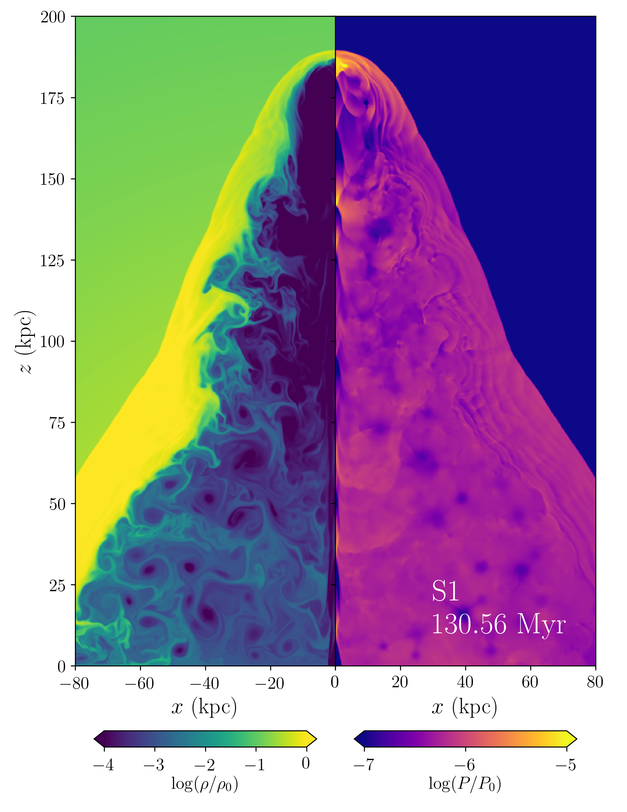
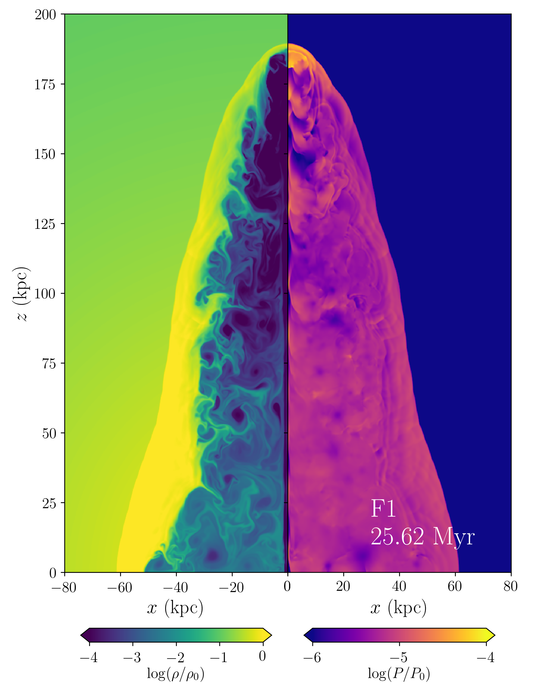
Figure 1: Logarithm of density and pressure for a snapshot of the 2D simulations, S1 (left) and F1 (right). The plots are normalised to the simulation unit density ($\rho_{0}=6\times 10^{-27}$ g cm^-3) and pressure ($P_{0}=5.393\times 10^{-6}$ dyne cm^-2). The jet creates a low-density cocoon which is separated from the shocked ambient medium by a contact discontinuity. Sharp shock structures can be seen in the pressure plot.

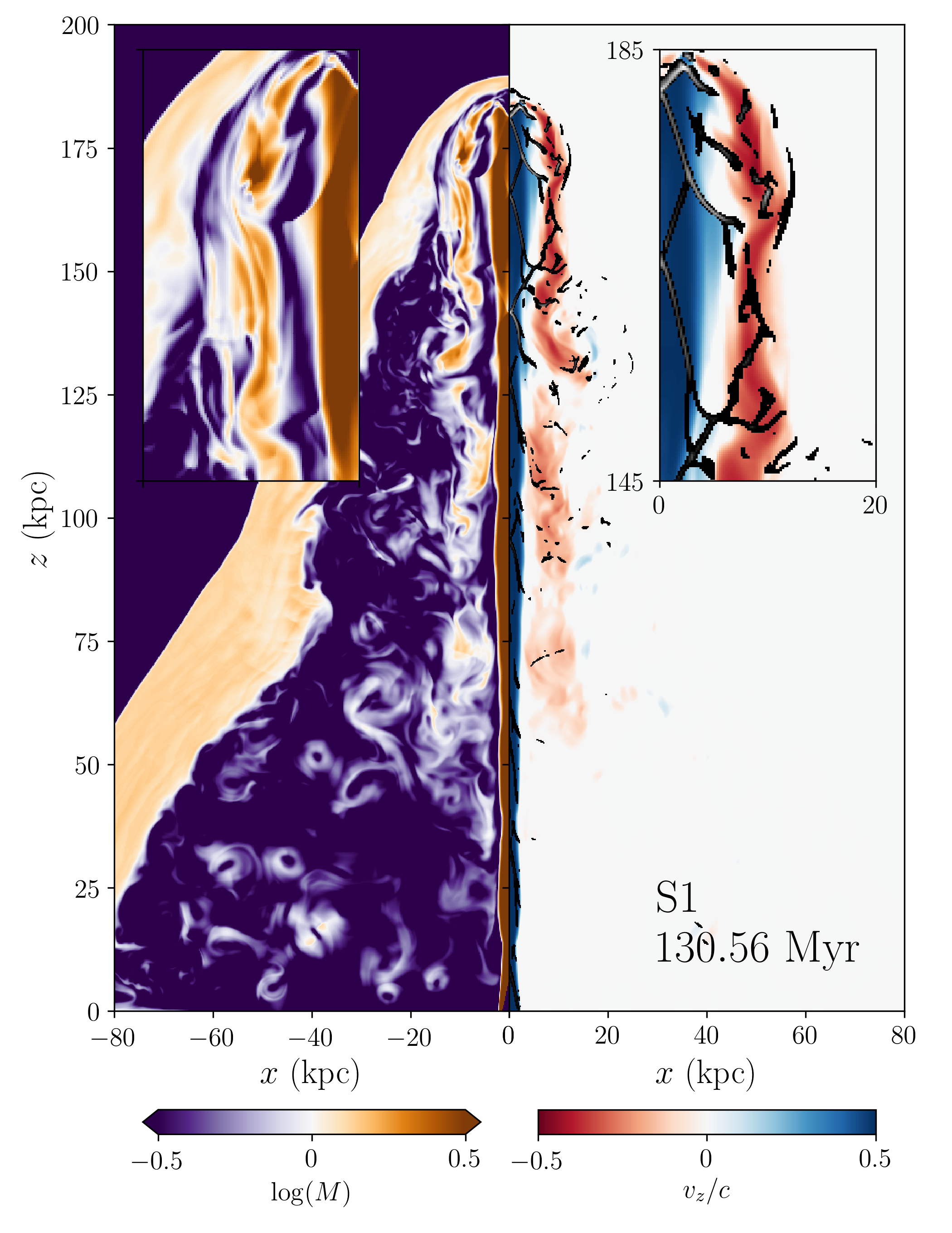
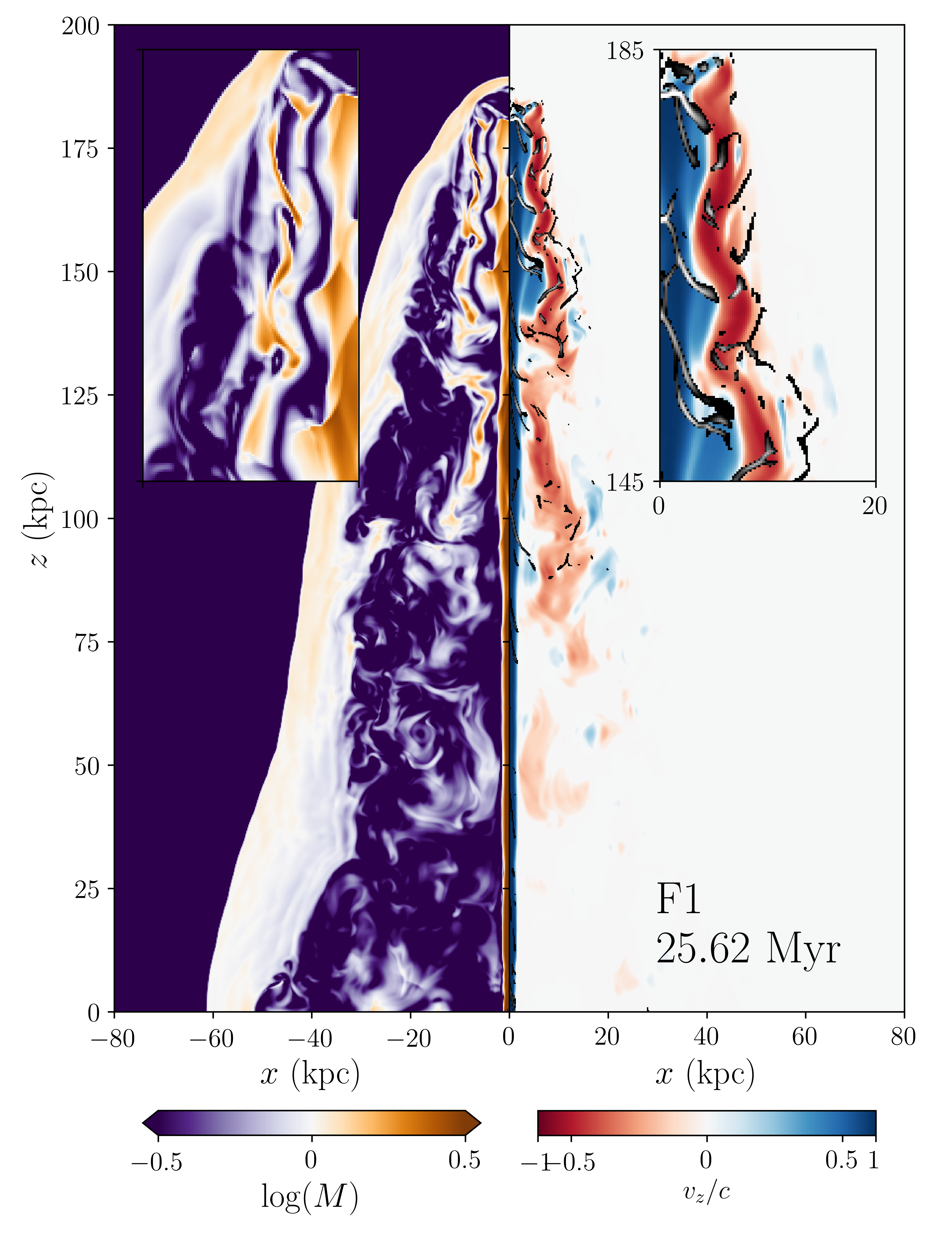
Figure 2: Logarithm of Mach number ($M$) and vertical velocity ($v_{z}$) for a snapshot of the 2D simulations, S1 (left) and F1 (right). In the $v_{z}$ plot, compression structures ($\nabla\cdot\boldsymbol{v}<0$) are coloured in grey to indicate shocks. Supersonic backflows form in both simulations and vortex shedding occurs from the jet head. Movies equivalent to these plots are included in the supplementary material as movS1Machvz.mp4 and movF1Machvz.mp4.

3.1 2D Simulations

Snapshots of the density and pressure for each of the 2D simulations are shown in Fig. 1. In each of the 2D plots we pick a time stamp at which the jet has travelled approximately $180$ kpc.The colourmaps are plotted logarithmically and normalised to the simulation unit density ($\rho_{0}=6\times 10^{-27}$g cm^-3) and pressure ($P_{0}=5.393\times 10^{-6}$dyne cm^-2). We show the S1 simulation at $130.56$ Myr and the F1 simulation at $25.62$ Myr. The jet is launched at high speed from the base of the grid ($z=0$) and encounters a series of reconfinement shocks as it propagates in the $z$ direction. This leads to the Mach number inside the jet dropping from its initial high value of $10^{10}$ to below $10$, although it still maintains a high speed close to its initial launch velocity. The jet deposits its mechanical energy at a termination shock, forming a hot spot. The jet material then inflates a low density cocoon. The cocoon and hotspot are significantly overpressured with respect to the surroundings and so the classic ‘double-shock’ structure is formed, with a bow shock propagating into the surrounding ambient medium. The shocked ambient material is separated from the shocked jet material by a contact discontinuity (CD), although mixing at this CD occurs via the Kelvin-Helmholtz instability as well as numerical viscosity on the grid scale ($0.2$ kpc in the 2D runs).

In Fig. 2 we show the Mach number, $M$, and $z$ (vertical) component of the velocity, $v_{z}$. In the velocity plot we also highlight compression structures in the flow; pixels are set to a greyscale if, in simulation units of $(c/\mathrm{kpc})$, $\nabla\cdot\boldsymbol{v}<-0.05$ (F1) or $\nabla\cdot\boldsymbol{v}<-0.02$ (S1), but otherwise are transparent so that the underlying velocity field can be seen. The compression structures help highlight the shocks in the simulation, which can also be seen to a lesser extent in the pressure plot in Fig. 1. Oblique reconfinement shocks can be seen clearly up the length of the jet, as well as a clear termination shock at the jet head. Although the flow is initially subsonic after the termination shock, it is funnelled sideways and backwards, where it becomes supersonic again, producing a number of moderately strong shocks. Although Fig. 2 is for a single snapshot, the movies in the supplementary material along with the 3D volume renderings (section 3.2) and tracer particle analysis (section 5.3) make clear that both the supersonic backflow and associated shock structures persist throughout the jet’s evolution.

3.2 3D Simulations

The 3D simulation (F3D) shows similar behaviour to the 2D simulations, but with some notable differences. To visualise the simulations, we show volume renderings of $v_{z}$ and $\log M$ in Figs. 3 and 4. The volume renderings are produced using composite ray-casting in Visit (Childs et al., 2005). In Fig. 3, the opacity is set linearly by $C_{j}$, whereas in Fig. 4 the opacity is set linearly by the kinetic energy flux, $\rho v^{3}/2$. We also show a visualisation of shock structures in Fig 5, where cells are opaque if they have a pressure gradient of $\tilde{\nabla}{P}/P>0.2$ and $\nabla\cdot\boldsymbol{v}<-0.05(c/\mathrm{kpc})$. The colour-coding discriminates between shocks in the jet (cyan) and shocks in the lobe or cocoon (orange). All our volume renderings are shown at four different times so the time evolution of the jet can be seen.

The 3D jets propagate more or less uninterrupted to the jet head, where they terminate in a similar manner to the 2D runs. The density perturbations ensure that the otherwise expected n=4 rotational symmetry is broken, leading to a complex flow structure in the lobe. Fast, supersonic backflows form. These backflowing streams mirror the 2D results in that their velocities can be a significant fraction (up to about half) of the jet velocity, and they persist when the jet has travelled far from the reflective/inflow boundary at $z=0$. However, the backflows can form streams of a helical shape, breaking cylindrical symmetry. This is important, as it means that the energy flux is focused into a smaller cross-sectional area, which can enhance the strength of any shock structures that form. The fraction of the jet power passing through the shock is important in determining the maximum CR energy (see section 7.1).

We can gain more insight into the geometry and strength of the backflow in 3D by taking slices in the $x-y$ plane at a few different values of $z$. Slices of $v_{z}$, $\log(M)$ and kinetic energy flux, $\rho v^{3}/2$, are shown in Fig. 6 for the F3D run at a time stamp of $26.11$ Myr. The plots show cylindrical symmetry to an extent, but a degree of focusing into asymmetric streams occurs. In reality, the exact degree of asymmetry may depend on the environment of the jet and the variation in launch direction, which highlights the importance of simulations that take into account more realistic cluster ‘weather’ (e.g. Mendygral et al., 2012). These plots make clear that, although a simplification, the 2D simulations in cylindrical symmetry offer a fairly good approximation to the 3D physics, so we just focus on the simpler 2D simulations for our Lagrangian shock analysis, particular as the focusing of the streams suggests that the cylindrically symmetric approximation is conservative if anything. However, a more detailed analysis of 3D simulations is potentially important and should be investigated. We do however analyse the shock sizes in our 3D simulation.

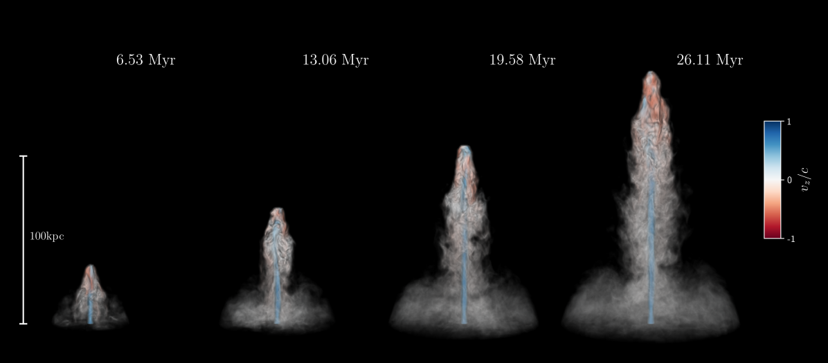
Figure 3: Volume rendering of the fiducial fast 3D simulation, F3D, showing $v_{z}$, the vertical component of velocity at four different times (labelled). The opacity is set linearly by the jet tracer, $C_{j}$. A movie equivalent to this plot is included in the supplementary material as movF3Dvz.mp4.

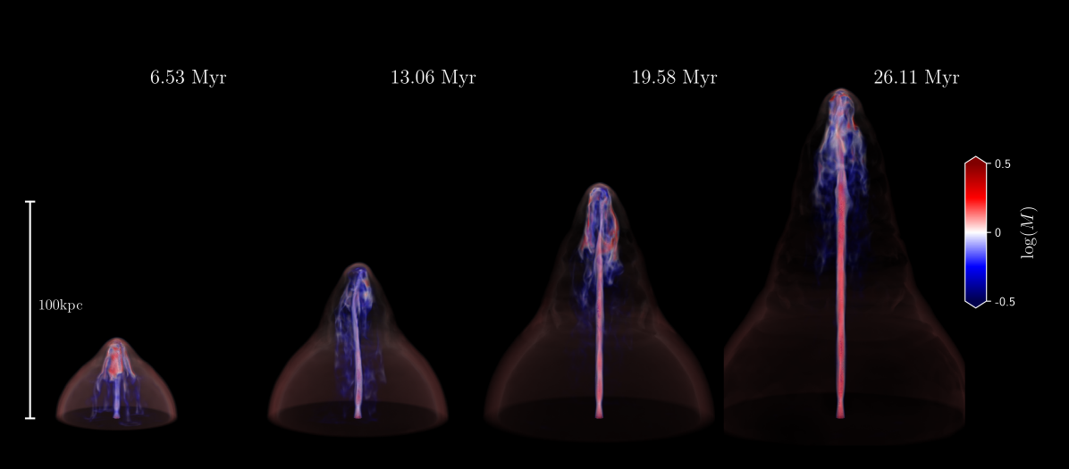
Figure 4: Volume rendering of the fiducial fast 3D simulation, F3D, showing $\log(M)$, the logarithm of the Mach number. Supersonic flow is coloured red. The opacity is set linearly by the kinetic energy flux, $1/2\rho v^{3}$, so that the areas in which the kinetic energy is focussed can be seen most clearly. A movie equivalent to this plot is included in the supplementary material as movF3DMach.mp4.

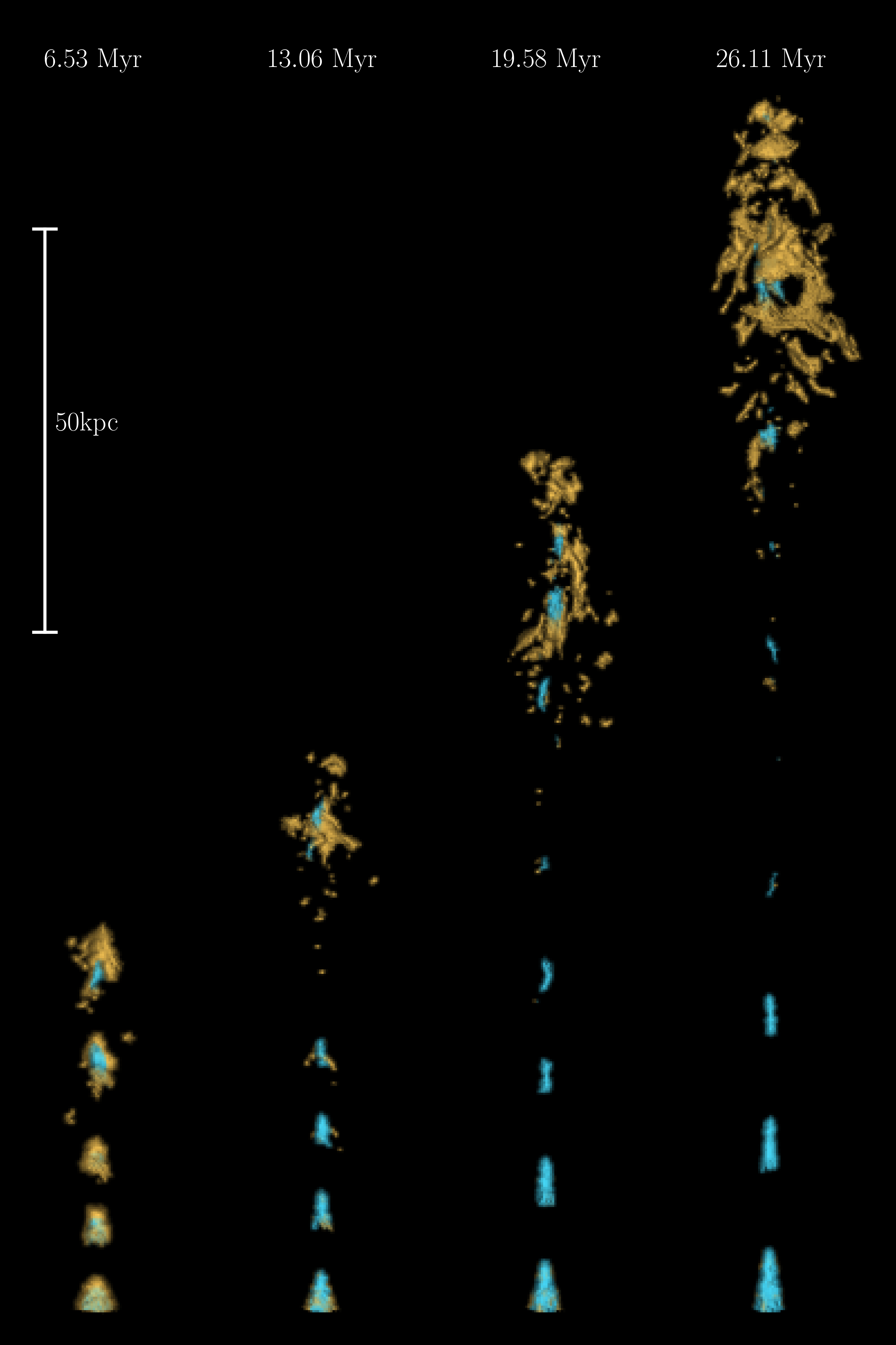
Figure 5: Volume rendering of the fiducial fast 3D simulation, F3D, showing shock regions. Regions are transparent against a black background unless they satisfy $\tilde{\nabla}{P}/P>0.2$ and $\nabla\cdot\boldsymbol{v}<-0.05(c/\mathrm{kpc})$, in which case they have an opacity of 1. Shocks are coloured cyan if they lie within the jet, and orange if they lie within the lobe or cocoon. The reconfinement shocks along the jet axes can be clearly seen, and there are a number of additional shocks in the lobe region, similarly to the 2D simulations (see Fig. 2).

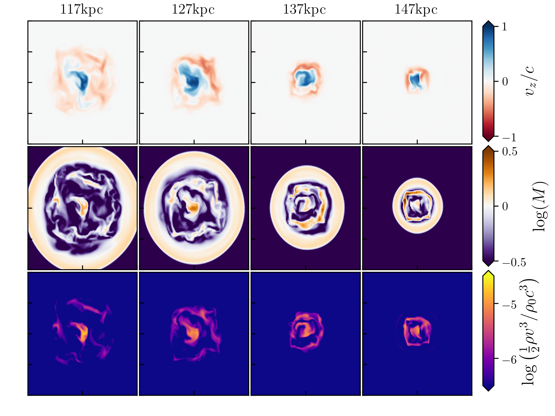
Figure 6: Slices in the $x-y$ plane of $z$ velocity component, Mach number and kinetic energy flux for the F3D simulation at a timestamp of $26.11$ Myr. The slices are $40\mathrm{kpc}\times 40\mathrm{kpc}$ and are taken at $10$ kpc intervals when the jet bow shock has advanced approximately $150$ kpc from the injection point. The kinetic energy flux is plotted in simulation units ($\rho_{0}c^{3}$).

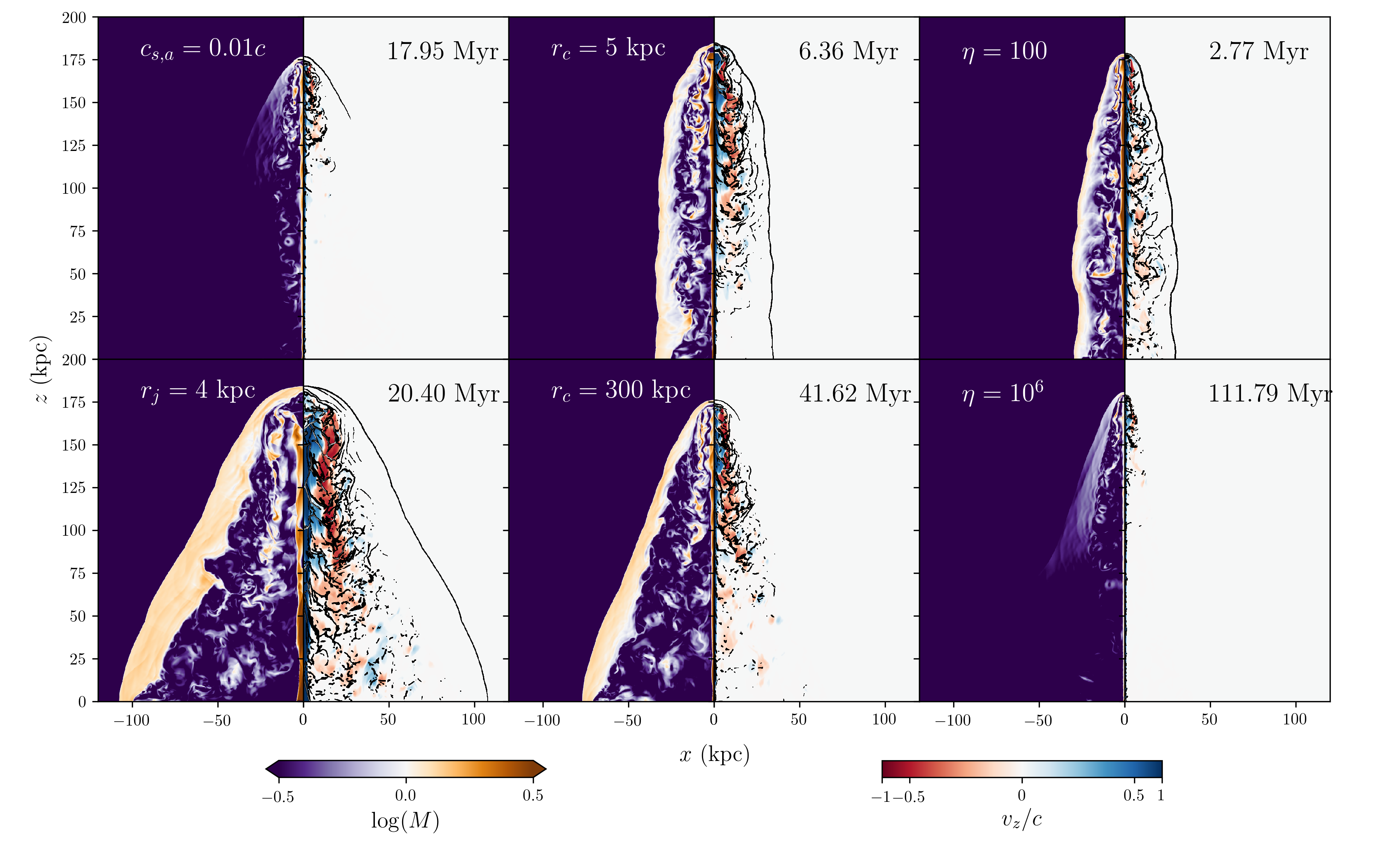
Figure 7: The effect of varying input parameters on the Mach number of the backflow. Analogues to Fig. 2 are shown for 6 separate runs where one parameter is varied with respect to the F1 simulation. The parameter in question and the simulation time is marked in each panel. Advance speeds and morphologies are varied, but while the details of the backflows change, they remain at least partially fast and supersonic in all cases.

3.3 Parameter sensitivity

It is important to know if the formation of fast, supersonic backflows is limited to our chosen region of parameter space. A comprehensive exploration of parameter space and the resultant backflow dynamics would make for interesting future work, but this is beyond the scope of the current study. However, to briefly highlight the impact of some important parameters on the jet dynamics and morphology, we explore the effect of varying $\eta_{r}$, $c_{s,a}$, $r_{c}$ and $r_{j}$. Taking the F1 simulation as our starting point, we vary each of these parameters in turn and show the Mach number and $v_{z}$ in Fig. 7. We choose the simulation time such that the jet has travelled approximately 150kpc in each case. The parameters chosen can change the aspect ratio and advance speeds, but in each case fast supersonic backflows form and we observe a similar qualitative behaviour to the F1 simulation. The length and width of the backflow is also affected by varying these parameters, but the prevalence of backflows is not limited to a specific case. In the next section, we will discuss the physical conditions under which we expect backflows to form, with further discussion of the advance speed and jet morphology.

4 Dynamics and morphology of the jet, backflow and lobe

Backflows in jet cocoons have been discussed in analytic and self-similar models (Falle, 1991; Scheuer, 1995) and observed in the earliest jet simulations (Norman et al., 1982). The strength of the backflows in the simulations of Norman et al. (1982) may be artificially enhanced by adopting outflow boundary conditions at $z=0$ outside the jet nozzle (Koessl & Mueller, 1988), but backflows nonetheless persist in a number of 3D HD and MHD simulations with more realistic boundary conditions (Saxton et al., 2002; Gaibler et al., 2009; Mathews & Guo, 2012; Mathews, 2014; Cielo et al., 2014; Tchekhovskoy & Bromberg, 2016). The presence of strong backflows in observations has also been inferred in a number of studies (Laing & Bridle, 2012; Mathews, 2014). Here, we examine the physical requirements for backflow and compare them to constraints from the jet morphology and dynamics.

4.1 When do backflows form?

We can gain some insight into the behaviour of the plasma in the backflowing region by considering Bernoulli’s principle, as applied to backflows from jets by Norman et al. (1982) and Williams (1991). Following Williams (1991), we consider a fluid parcel that has passed through the termination shock and has a velocity $v_{h}$, density, $\rho_{h}$, and a pressure, $P_{h}$, directly downstream of the shock, set by the shock jump conditions. The fluid parcel is funnelled sideways and backwards away from the hotspot. We now assume steady flow and consider the velocities in the frame of the termination shock (which is moving slowly in the observer frame if the density contrast is high). Neglecting gravity, we can use the non-relativistic steady-state momentum equation, $\boldsymbol{v}\cdot\nabla\boldsymbol{v}=-\nabla P/\rho$, and make use of the identity $\boldsymbol{v}\cdot\nabla\boldsymbol{v}=\nabla(v^{2}/2)-\boldsymbol{v}\times(\nabla\times\boldsymbol{v})$ and the adiabatic condition $P\rho^{-\gamma}=P_{h}\rho_{h}^{-\gamma}$ to write

$$\nabla\left(\frac{v^{2}}{2}+\frac{\gamma}{\gamma-1}\frac{P_{h}^{1/\gamma}P^{(\gamma-1)/\gamma}}{\rho_{h}}\right)-\boldsymbol{v}\times(\nabla\times\boldsymbol{v})=0.$$ (12)

We can now integrate along a streamline of steady flow to give a conserved, Bernoulli-like quantity

$$\chi=v^{2}+\frac{2\gamma}{\gamma-1}\frac{P_{h}^{1/\gamma}P^{(\gamma-1)/\gamma}}{\rho_{h}}=v_{h}^{2}+\frac{2\gamma}{\gamma-1}\frac{P_{h}}{\rho_{h}}.$$ (13)

Under these assumptions the velocity $v$ will be maximum at a point along the streamline where $P$ is minimum. Thus, the backflow is maximised when the pressure difference between the cocoon and hotspot is highest. The jet is confined by the pressure in the cocoon and so is in rough pressure equilibrium with the cocoon far from the hotspot. We can therefore write an equation for the characteristic velocity of the backflow, $v_{b}$, under the additional assumption that $P\approx P_{j}$,

$$v_{b}=\left[v_{h}^{2}+\frac{2\gamma}{\gamma-1}\frac{P_{h}}{\rho_{h}}-\frac{2\gamma}{\gamma-1}\frac{P_{h}^{1/\gamma}P_{j}^{(\gamma-1)/\gamma}}{\rho_{h}}\right]^{1/2}$$ (14)

since $P_{h}$ is set by the termination shock jump conditions and is proportional to $\rho_{j}v_{j}^{2}$, the backflow speed is maximised when the jet Mach number is high. If we now for simplicity assume non-relativistic jump conditions at the termination shock and set $\gamma=5/3$ we have $P_{h}=3\rho_{h}v_{h}^{2}$ and therefore the Mach number of the flow is given by

$$M^{2}=\frac{1}{5}+\frac{16}{5}\left[\left(\frac{P}{P_{h}}+1\right)^{-2/5}\right].$$ (15)

In this (illustrative) non-relativistic limit, the flow goes supersonic when $P\approx 0.57P_{h}$ and $v\rightarrow v_{j}$ if $P\rightarrow 0$.

The above analysis shows that as long as the pressure in the stream is allowed to drop below a critical value then the flow must go supersonic. The pressure in the backflowing stream is governed by the pressure variations in the turbulent lobe, so there is a complicated interaction between the collimation of this stream and the surrounding medium. The speed and Mach number of the backflow are both maximised when the jet Mach number is high and when the jet is light with respect to its surroundings, as shown by other authors (e.g. Norman et al., 1982; Williams, 1991). Once the backflow is supersonic, the only way it can slow down is via shocks; hence, shocks are an inevitable feature of backflows in astrophysical jets.

The backflows shown in the $x-y$ slices in Fig. 6 are supersonic, fast and radially thin compared to $r_{j}$. This behaviour is expected. Since much of the jet material is funneled along the backflow, conservation of mass in rough cylindrical symmetry gives $\pi r_{j}^{2}\rho_{j}v_{j}\sim 2\pi r_{b}w_{b}\rho_{b}v_{b}$, where $r_{b}$ is the radial distance of the backflow from the jet axis and $w_{b}$ is the radial width of the backflowing stream. Since $r_{b}>r_{j}$, as the pressure drops and $v_{b}$ increases the backflow becomes a thin, supersonic stream along which a large fraction of the jet’s kinetic energy flux can be focused.

4.2 Advance speed and aspect ratio

Two important empirical measurements that place constraints on jet physics are the advance speed of the jet head, $v_{\mathrm{head}}$, and the aspect ratio of the jet width to cocoon width, $A=R_{c}/R_{j}$. Advance speeds of FRII sources are generally much lower than the jet velocity, often on the order of $0.01c$ for relativistic jets (Scheuer, 1995; Carilli & Barthel, 1996; Blundell et al., 1999, e.g). The advance speed of the jet head, $v_{\mathrm{head}}$ is governed by the jet velocity $v_{j}$ and the relativistic jet density ratio, $\eta_{r}$, and from 1D ram pressure balance one obtains (Marti et al., 1997)

$$v_{\mathrm{head}}=\frac{\sqrt{\eta_{r}}}{\sqrt{\eta_{r}}+1}v_{j}.$$ (16)

The relativistic generalisation of the jet density ratio increases rapidly for high $\Gamma_{j}$ ($\eta_{r}\propto\Gamma_{j}^{2}$, see equation 7). Thus, it is quite difficult to arrange that a steady, light jet has high kinetic power but a relatively slow advance speed. In reality, the intermittency of the jet may be crucial in delivering power down the jet nozzle without the average advance speed increasing dramatically, but a study of this is beyond the scope of this paper.

We can also estimate the physical dependence of $A$, which will allow us to check if backflows should only occur in jets with certain morphologies. In FRII radio galaxies this ratio is generally quite large (Williams, 1991; Krause, 2005; English et al., 2016) – a ratio of $\sim 30$ can be inferred from radio images of Cygnus A (Perley et al., 1984). An approximate estimate of $A$ can be derived for a uniform ambient medium if we model the cocoon as a cylinder of radius $R_{c}$ expanding in length at a rate $v_{\mathrm{head}}$, then the rate of energy change in this cylinder is $\pi R_{c}^{2}v_{\mathrm{head}}U_{c}$, where we assume a constant internal energy density $U_{c}$. If we equate this to the jet power $Q_{j}$ from equation 8 and make the additional assumption that $P_{j}=P_{c}$ then we obtain

$$A=\frac{R_{c}}{R_{j}}=\left[\frac{\Gamma_{j}(\Gamma_{j}-1)\rho_{j}c^{2}+\frac{\gamma}{\gamma-1}\Gamma_{j}^{2}P_{j}}{2(\gamma-1)P_{j}}\frac{v_{j}}{v_{\mathrm{head}}}\right]^{1/2},$$ (17)

which makes it clear that wider cocoons compared to the jet width are preferentially produced by slow advance speeds and high Mach number jets, as shown by Williams (1991). Even if the assumption of $P_{j}=P_{c}$ is dropped, large values of $A$ still occur when the pressure in the jet hotspot is large compared to the average pressure in the cocoon. Intermittency, or “dentist-drill” variability (Scheuer, 1982), can also increase this aspect ratio, as has been shown in simulations of intermittent jets (e.g. Tchekhovskoy & Bromberg, 2016).

Overall, the empirical evidence points towards wide cocoons and slow advance speeds, which favours light, high Mach number jets (equations 16 and 17). These are also the conditions in which strong backflows are produced (equation 14), which, together with the ubiquity of backflows for all parameters explored in section 3.3, allows us to conclude that backflows are not unique to our particular parameter space but instead should exist in a large fraction of powerful extragalactic radio sources.

4.3 The effect of magnetic fields

Neither our HD simulations, nor the Bernoulli argument above, accounts for the effects of the magnetic field. The magnetic field helps determine the maximum CR energy (see section 6.1) but can also affect the jet confinement and the dynamics of the lobe. MHD simulations of AGN jets show various behaviours depending on the field topology and magnetization parameter $\sigma$, which is the ratio of the Poynting flux to kinetic energy flux in the jet frame. High $\sigma$ simulations can suppress backflow, instead forming a ‘nose cone’ of material being collected ahead of the termination shock (Clarke et al., 1986; Komissarov, 1999; Gaibler et al., 2009), although this does not occur for purely poloidal fields (Leismann et al., 2005). However, while the jet is expected to be Poynting flux dominated near the jet base (e.g. Beskin et al., 2011; Zdziarski et al., 2015), such jets will likely become kinetically dominated beyond kpc scales (Appl & Camenzind, 1988; Sikora et al., 2005). A transition to kinetic energy dominance can be caused by the magnetic kink instability (Appl et al., 2000), as shown by (e.g. Giannios & Spruit, 2006; Tchekhovskoy & Bromberg, 2016). Furthermore, observations of radio galaxies such as Cygnus A and Pictor A show extensive cocoons rather than a nose cone morphology (e.g. Perley et al., 1984; Hardcastle & Croston, 2005), suggesting backflows are present.

In lower $\sigma$ simulations, which produce a good match to observations (Hardcastle & Krause, 2014), the magnetic field can still affect the jet and lobe dynamics. Gaibler et al. (2009) find that helical magnetic fields in the jet can alter the advance speed (which could lead to lower values of $A$ than from equation 17), damp Kelvin-Helmholtz instabilities and widen the jet head. Keppens et al. (2008) find interesting behaviour in the backflow region, where a compressed magnetic field between the backflow and jet can suppress the interaction between the two. Magnetic confinement of the jet (Begelman et al., 1984) may also alter the Bernoulli argument above, and change the partitioning of energy densities in the lobe needed to confine the jet by a numerical factor depending on the field topology. Overall, the dynamic impact of the magnetic field on the backflow certainly warrants further attention (see also section 6.1), but is unlikely to change our general arguments.

5 Shock properties

To examine shock properties we use an Eulerian method to calculate the shock size and Lagrangian tracer particles to measure the distribution of shock Mach numbers and velocities that fluid elements pass through. We limit the range of times within which we analyse shocks so that the first time stamp analysed corresponds to when the jet has advanced approximately $50$ kpc. This results in time ranges of $35.9$-$122.4$ Myr, $6.2$-$40.8$ Myr and $6.2$-$32.64$ Myr for the S1, F1 and F3D simulations, respectively. All histograms relating to Lagrangian tracer particles are normalised to the number of tracer particles injected during these time ranges, which we denote $N_{\mathrm{p,tot}}$.

5.1 Eulerian shock statistics

To calculate shock size $r_{\rm s}$, we first flag grid cells as inside shocks if they satisfy the conditions $\tilde{\nabla}P/P>0.2$ and $\nabla\cdot\boldsymbol{v}<-0.05(c/\mathrm{kpc})$. We also impose the additional constraints of $C_{j}>0$ and $x>2$, in order to focus on the jet lobe and cocoon. We then make use the scikit-learn (Pedregosa et al., 2011) implementation of the Density-Based Spatial Clustering of Applications with Noise (DBSCAN) algorithm (Ester et al., 1996) to identify shock regions. We call the cluster.DBSCAN function in scikit-learn, setting min_samples=5 and eps=2. This means that the smallest number of grid cells that constitute a cluster is 5, while the shortest distance between two points in a cluster is twice the grid scale.

Once the shock clusters have been identified, we calculate the shock size by measuring the linear extent of each identified cluster and assuming (conservatively) a straight shock. A histogram of shock sizes is shown in Fig. 8. We find shock sizes ranging from just above the grid resolution up to nearly $10$kpc. For the 2D simulations, we only calculate the shock size in the $x-z$ plane rather than measuring the cylindrical extent of the shock, although in 3D the shock size is calculated in 3D and the slightly larger shock size is indicative of the partial ring shapes formed by the backflowing streams shown in Fig. 6. The mean shock sizes in the S1, F1, and F3D simulations are $2.01$ kpc, $1.85$ kpc and $4.61$ kpc, respectively; we therefore take $2$ kpc as a typical shock size.

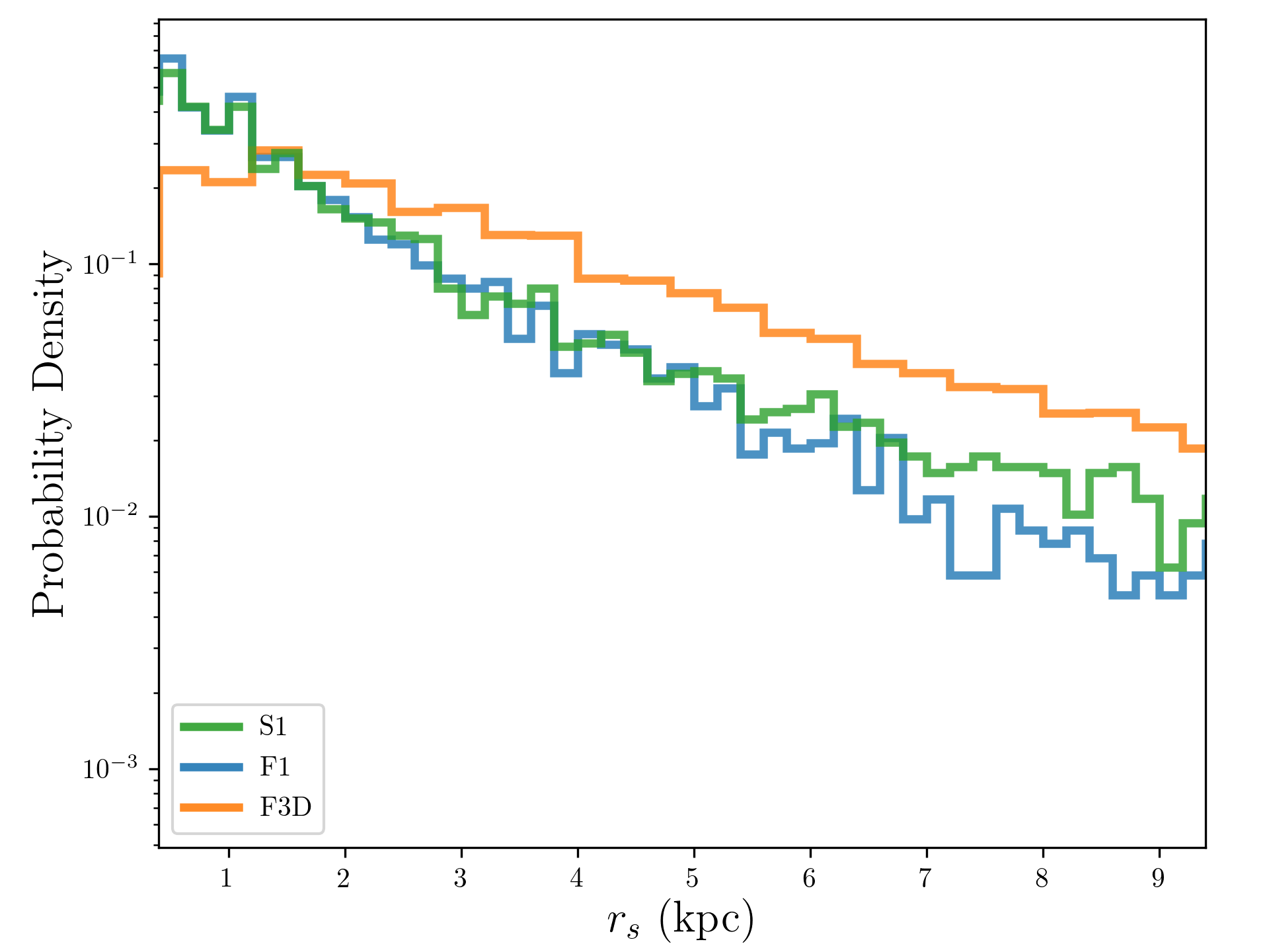
Figure 8: Histogram of shock sizes in kpc from the S1, F1 and F3D simulations, as described in section 5.1. The histogram is in units of probability density.

5.2 Tracer particle histories

Tracer particles are injected in the 2D simulations at the jet nozzle as described in section 2.3. We record the local fluid properties for each particle as it is advected with the flow, writing to file every $\Delta t=3,264$ yr (1 simulation time unit). The trajectories of 100 random tracer particles are shown in the left-hand panel of Fig. 9, colour-coded by launch time, showing that the tracer particles propagate along the jet before invariably being channeled along backflowing streams. The vorticity in the backflow and further into the cocoon manifests as loops and twisting patterns in the trajectories of the particles.

The right hand panel of Fig. 9 shows trajectories for 8 individual tracer particles, while profiles of some key quantities as a function of distance travelled by the same tracer particles are shown in Fig. 10. We show the logarithm of $M$ and linear profiles of $(\Delta P/P)_{L}$ and $v_{z}$, with distance travelled normalised to $r_{\mathrm{turn}}$, the distance at which the sign of $v_{z}$ first becomes negative. The particles travel along the jet and pass through a series of reconfinement shocks. These reconfinement shocks can be seen in the colormaps in section 3 and they show up as clear spikes in $(\Delta P/P)_{L}$ in the tracer profiles. This acts as a verification of this quantity as a shock diagnostic. The reconfinement shocks cause the internal Mach number to drop, as expected, although the fluid generally remains supersonic, with $v_{z}$ close to its initial value of $0.95c$, until the jet terminates. At this point, there is usually a clear drop in $v_{z}$ and $M$. Shortly after this point, the sign of $v_{z}$ can become negative showing that the tracer particle has entered a backflowing stream. The Mach number can increase again in the backflow, and subsequent shocks are often encountered. After a time, the material is advected deep into the cocoon and comes into rough pressure equilibrium with the larger-scale surroundings. Turbulence and vorticity persist throughout this cocoon, but far from the hotspot the flow is generally subsonic, although occasionally transonic (see also Fig. 2).

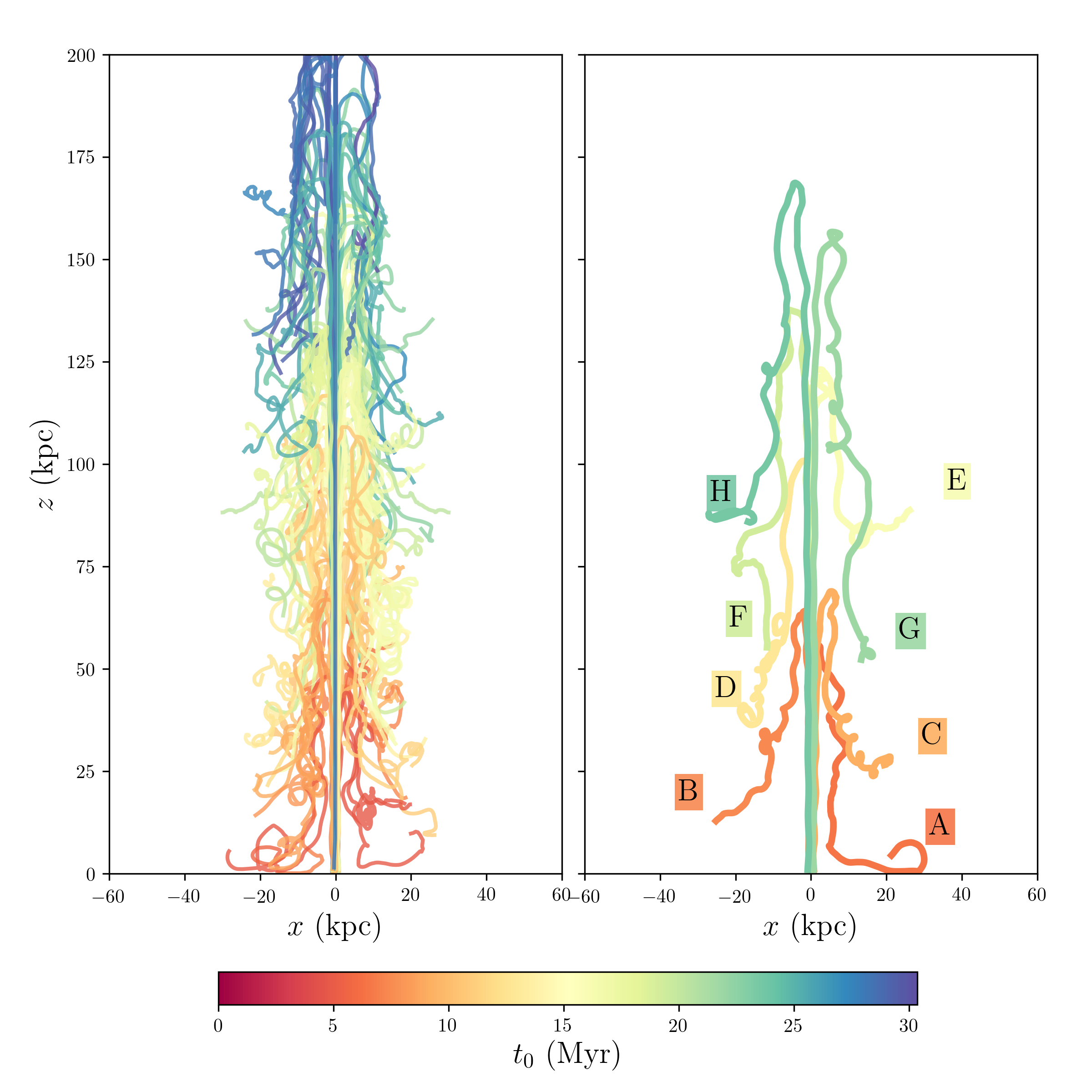
Figure 9: Left: Tracer particle trajectories from the F3d simulation for 100 random tracer particles, with the sign of the $x$-coordinate also chosen randomly. The colour corresponds to the launch time of the particle, $t_{0}$, in Myr. Right: Trajectories for 8 individual tracer particles whose histories are shown in Fig. 10. The colour scheme is identical to the left panel and the labeled letters match those in Fig. 10.

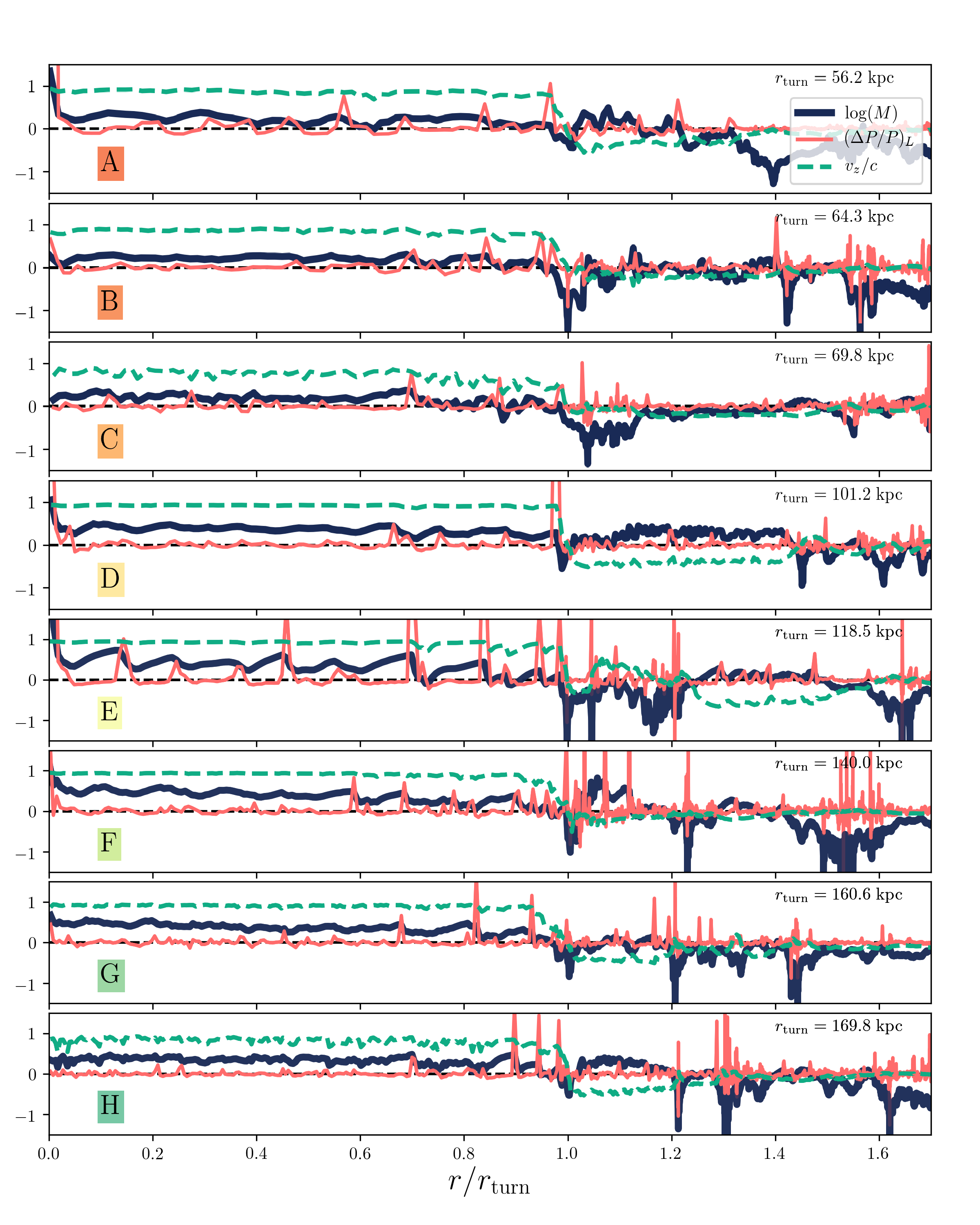
Figure 10: Profiles of $\log(M)$, $(\Delta P/P)_{L}$ and $v_{z}$ for eight Lagrangian tracer particles in the F1 (2D) simulation. The distances travelled by the particles, $r$, are normalised to the distance travelled at the first point when the $z$-component of the velocity of the local fluid has become negative ($r_{\mathrm{turn}}$) – the “turning point” after which the particle is then travelling along the backflow. While $v_{z}$ illustrates when the particle enters the backflow, $\log(M)$ and $(\Delta P/P)_{L}$ show supersonic flow and shocks. The labels in each panel match those in Fig. 9.

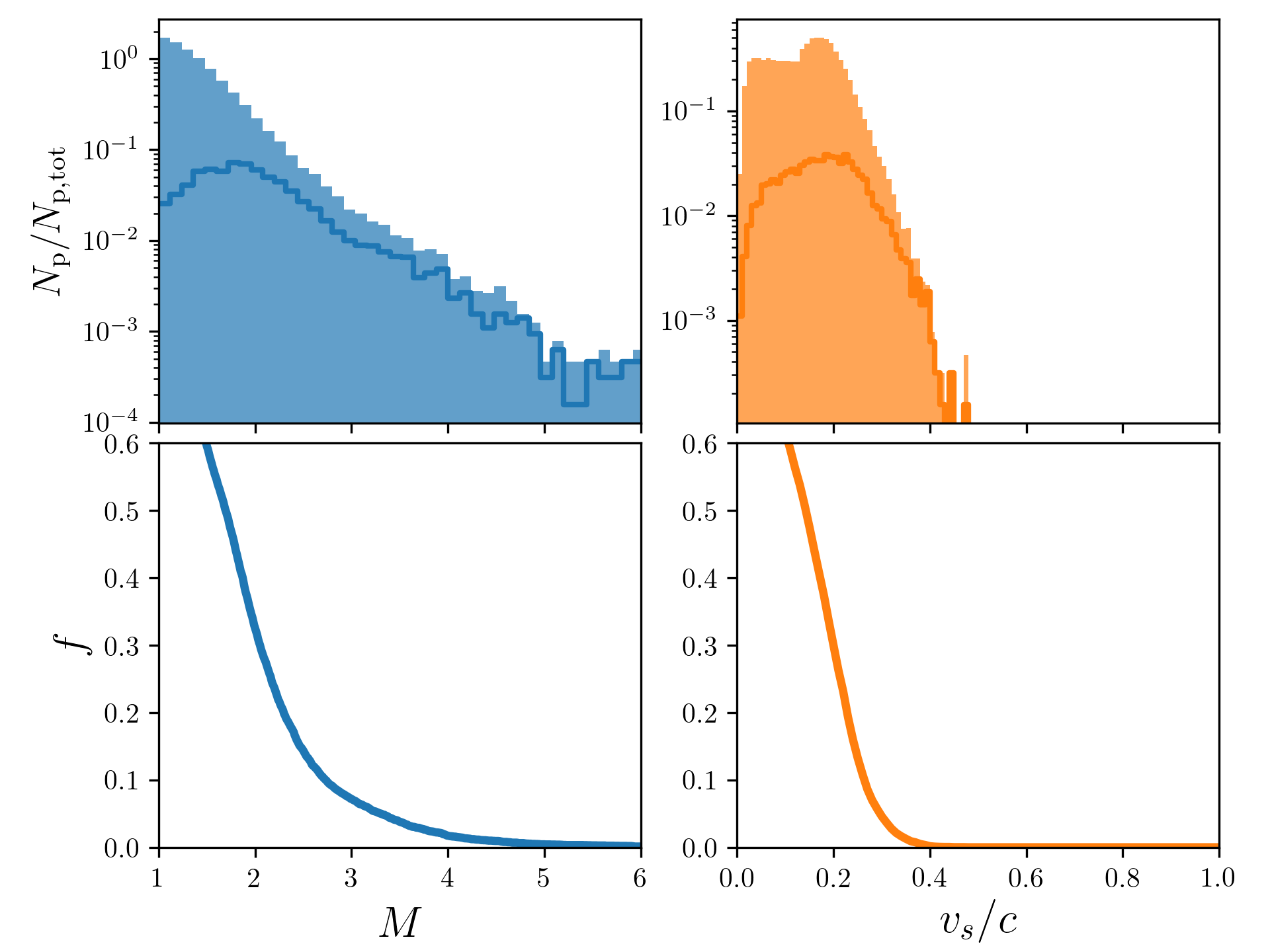
(a) Shock properties in run S1

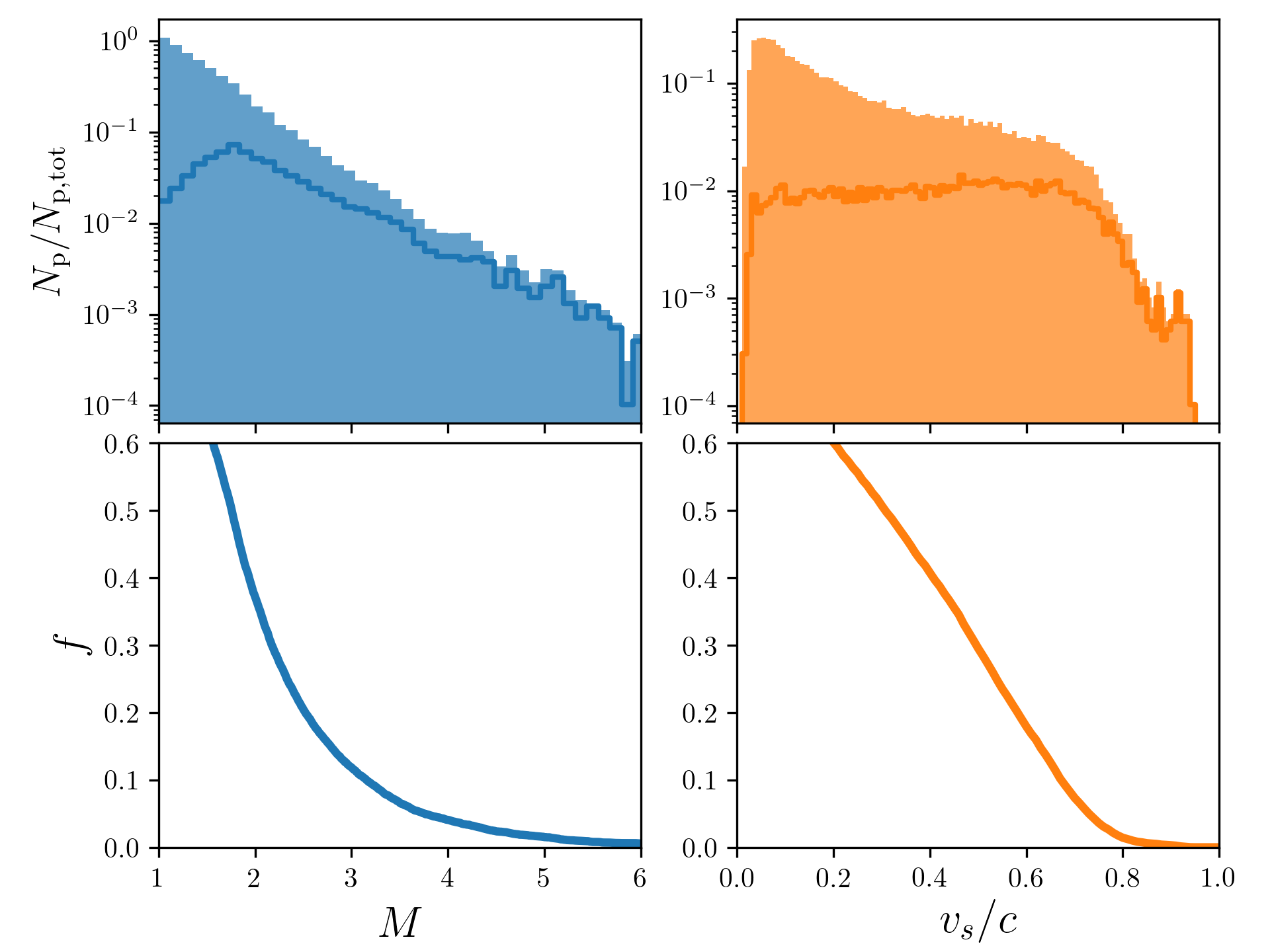
(b) Shock properties in run F1

Figure 11: Shock Mach numbers and velocities as recorded by the Lagrangian tracer particles for both of the 2D simulations (S1 and F1). Top two panels: histograms of $M$ (left) and $v_{s}/c$ (right) the shocks passed through by all tracer particles within the time range considered. The solid histogram shows all shocks, while the solid line shows only the strongest shock that each particle passes through. Bottom left: The fraction of particles passing through a shock with Mach number as least as high as $M$; this is equal to one minus the cumulative distribution function (CDF) of the solid line in the panel above. Bottom right: The fraction of particles whose strongest shock has a velocity of at least $v_{s}$.

5.3 Lagrangian shock statistics

The tracer particle histories shown in Figs. 9 and 10 give some idea of the shocks a fluid element might pass through in the backflow, but it is important to analyse this data statistically. Specifically, we are concerned with the percentage of tracer particles that pass through strong shocks with the right kind of shock velocities. We do this by identifying shocks as described previously by requiring $(\Delta P/P)_{L}<0.2$, $\nabla\cdot\boldsymbol{v}<-0.05(c/\mathrm{kpc})$, $C_{j}>0$ and $x>2$. We also only record the shocks that have occurred once the tracer particle has entered the backflow, i.e. after the $z$-component of the velocity of the local fluid has first become negative (see Fig. 10). We record the properties ($M,v_{s}$) of each shock that each tracer particle passes through. The most important shock is the strongest one, since that will tend to have the flattest spectrum (Blandford & Eichler, 1987) and will therefore dominate the UHECR contribution.

In Fig. 11 we show statistics for the Lagrangian tracer particles in both our 2D runs. We give the distributions of $M$ and $v_{s}$ for all shocks that the tracer particles pass through, as well as just the strongest shocks (highest $M$). We also show the fraction of particles that have passed through a shock at least as strong as $M$, which is equal to one minus the cumulative distribution function of the histograms in the top panel. These figures illustrate that in both cases approximately $10\%$ of particles pass through a shock of $M>3$. These shocks have a range of shock velocities and can be non-relativistic or mildly relativistic; we take $v_{s}=0.2c$ as a typical shock velocity.

5.3.1 Number of Shock Crossings by a fluid element

Multiple shocks occur along the backflow and throughout the cocoon, as can be seen in e.g. Figs 2. There is thus opportunity for fluid elements to cross multiple shocks. Fig. 12 shows a histogram of the number of shock crossings by the Lagrangian tracer particles in the F1 simulation, for two different Mach numbers. The histogram is normalised so that it shows the fraction of all tracer particles passing through $N_{\mathrm{s}}$ shocks. The tracer particles often pass through more than one additional shock downstream of the jet termination shock, as would be expected from the backflows seen in Figs 2 and 4. The percentage of particles passing through two or more $M>3$ shocks in the F1 simulation is $4.96\%$, compared to the $11.8\%$ of particles that pass through at least one $M>3$ shock.

A particle passing through a number of shocks can be further accelerated and the final CR-spectrum is harder than in a single shock acceleration (Bell, 1978b; Blandford & Ostriker, 1980; Achterberg, 1990; Pope & Melrose, 1994; Melrose & Crouch, 1997; Marcowith & Kirk, 1999; Gieseler & Jones, 2000). The situation in the backflow is therefore similar to that considered by Meli & Biermann (2013), except that their analysis concerns oblique reconfinement shocks in the jet. Multiple shock crossings make the overall conditions favourable for acceleration to high energy, as not only can existing CRs be further accelerated but the magnetic field has multiple opportunities for amplification. We discuss the latter further in section 6.1. Concerning the maximum energy of particles, the upper-limit is still set by the size of the shocks and the value of the magnetic field, as we describe in the next section, but $N_{s}$ shock crossings will make conditions more favourable and increase the maximum CR energy by a factor on the order $N_{s}$.

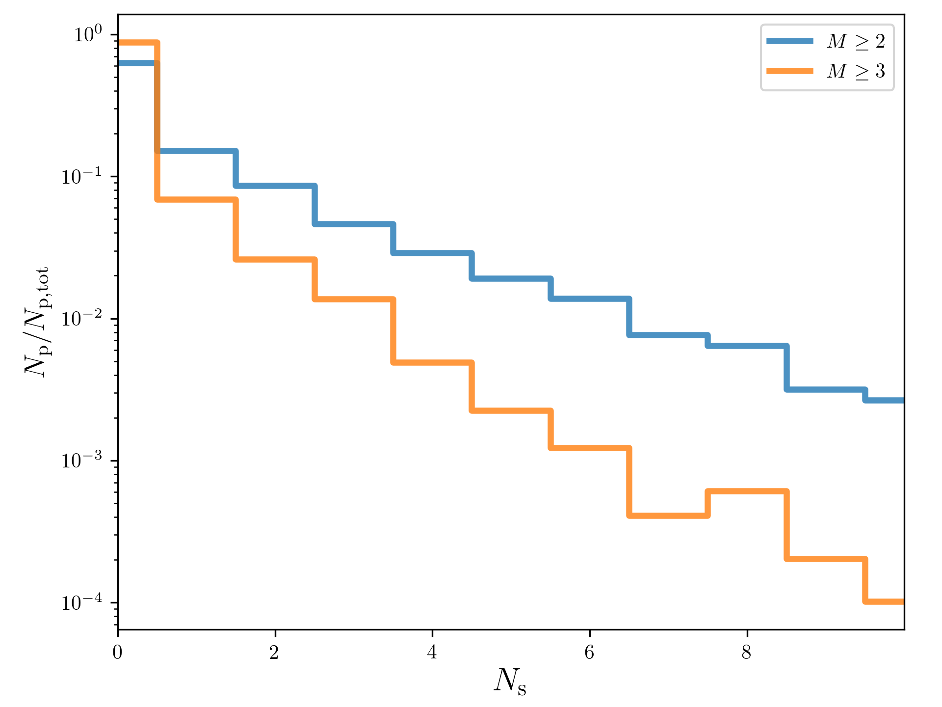
Figure 12: A histogram showing the number of shock crossings, $N_{\mathrm{s}}$ by a tracer particle in run F1, for two different shock Mach numbers. $N_{\mathrm{p}}$ is the number of particles passing through $N_{\mathrm{s}}$ shocks, while $N_{\mathrm{p,tot}}$ is the total number of tracer particles injected in the simulation.

6 Maximum Cosmic-Ray Energy

The Hillas energy, given by Eq. (1), sets the characteristic maximum energy achievable by a CR. To estimate $E_{H}$ we adopt values of $v_{\rm s}=0.2c$ and $r_{\rm s}=2$ kpc informed by the results of the previous section, but the appropriate value of the magnetic field $B$, as well as the composition of UHECRs (and therefore appropriate $Z$) is also crucial.

6.1 Magnetic Field

Our simulations are HD, rather than MHD, so we do not solve the induction equation. The reasoning for this is partly that the magnetic field that matters for accelerating CRs to high energy is the turbulent, amplified field at the shock, which is small-scale until it grows to the Larmor radii of the highest energy CRs. Furthermore, the amplification is driven by streaming or drifting CRs with a spectrum of energies, which grow the turbulence on a variety of scales. Instead of trying to resolve and self-consistently model the instabilities that amplify the field, we instead make some general arguments informed by plasma physics modelling and the acceleration of Galactic CRs by SNRs.

Turbulent magnetic field amplification is a general feature of any DSA theory (Bell, 1978a, b). Current-driven instabilities can amplify the field via a $\boldsymbol{j}_{\mathrm{ret}}\times\boldsymbol{B}$-force that stretches and distorts the field, where $\boldsymbol{j}_{\mathrm{ret}}$ is a return current produced in reaction to the CR current. At wavenumbers resonant with the Larmor radius of the CRs producing the current, this instability is known as the resonant or Alfvén instability (Lerche, 1967; Kulsrud & Pearce, 1969; Wentzel, 1974; Skilling, 1975a, c, b). The resonant instability can only amplify the field to $\delta B/B\sim 1$ (e.g. Amato & Blasi, 2009; Bell, 2014). The non-resonant hybrid (NRH) or Bell instability can amplify the magnetic field to many times its ambient value (Bell, 2004; Zirakashvili et al., 2008; Niemiec et al., 2008; Stroman et al., 2009; Riquelme & Spitkovsky, 2009; Bell et al., 2013) in the case of both parallel and perpendicular initial field orientations (Bell, 2005; Milosavljević & Nakar, 2006; Riquelme & Spitkovsky, 2010; Matthews et al., 2017).

Bell et al. (2018) showed that on small scales, within one UHECR Larmor radius of a highly relativistic (quasi-perpendicular) shock, the magnetic field is not amplified on a scale length large enough to scatter UHECRs. Similar arguments were applied to the hotspots of FRII radio galaxies, where the maximum energy of the electrons at the termination shock (hotspot) is set by the growth of turbulence on the scale of a Larmor radius in the perpendicular unperturbed magnetic field and not synchrotron cooling as was usually assumed (Araudo et al., 2016, 2018). The same constraint applies to protons and therefore the CR maximum energy is about 1 TeV, the same as the maximum electron energy inferred by the optical-IR synchrotron cutoff. In the particular case of the FRII radio galaxy Cygnus A, the magnetic field in the hotspot can be amplified to large values of $50-400~{}\mu$G, but not on the right scale for acceleration to EeV energies (Araudo et al., 2018).

Secondary shocks in the backflows of the jets have a number of advantages over the termination shock in terms of their prospects for UHECR production. These include:

1. they span a range of velocities and so they include non- and mildly relativistic shocks;

2. they occur after the termination shock and so can make use of the already amplified field as a small-scale seed field;

3. fluid elements can pass through multiple shocks providing multiple opportunities for acceleration and field amplification by CR streaming instabilities;

4. the magnetic field can be amplified by other mechanisms (e.g. vorticity) and not only CR-driven instabilities over Larmor radii scale lengths at the shock.

Point (i) is important in order to avoid the issues inherent to relativistic shocks described in detail by Bell et al. (2018). The final three points are crucial in terms of allowing the magnetic field to grow to the right scale and strength to accelerate UHECRs. In SNRs, the maximum CR energy is generally much lower than the Hillas energy, since one must take into account effects from the CR diffusion coefficient and system age (Lagage & Cesarsky, 1983) as well as the timescales and saturation fields associated with the amplification mechanism at the shock (Bell et al., 2013). If the magnetic field is amplified by the NRH instability then it saturates once the $\boldsymbol{j}\times\boldsymbol{B}$ force from the CR return current is balanced by magnetic tension, that is when $\mu_{0}\boldsymbol{j}\sim\nabla\times\boldsymbol{B}$. While this effect is not always restrictive (Bell et al., 2013), the effect of the magnetic energy density being spread over many decades in the scale size of the field can be. The result is that the fields measured in synchrotron observations of SNRs, typically $100$s of $\mu$G (Cassam-Chenaï et al., 2007; Uchiyama et al., 2007), cannot be naively substituted into the equation for the Hillas energy.

In jet backflows, the physical situation is fundamentally different to that in SNRs. Giacalone & Jokipii (2007) have shown that density perturbations, which are bound to exist in such a dynamic and variable environment, can cause the field to become amplified a long way downstream of the shock. This, along with the general vorticity expected in jet hotspots and their associated backflows (e.g. Norman et al., 1982; Falle, 1991) can stretch field lines, amplifying the field and allowing the scale length to grow to the Larmor radius of a UHECR. We therefore expect the maximum energy of particles accelerated in these backflow shocks – and any secondary shocks downstream of the termination shock – to be much closer to the Hillas energy than in SNRs. This is because there is more than one mechanism, and more than one opportunity, for the field to be amplified and stretched on the scale of an UHECR Larmor radius.

The qualitative picture we have outlined is physically motivated but requires further investigation. Much of the physics is “subgrid” level; a full treatment would require resolution spanning decades and is not feasible, although shock-tube style simulations designed to imitate a streamline might prove useful in terms of estimating the impact of vorticity and dynamo action on the turbulent field, as in e.g. Giacalone & Jokipii (2007). We note that De Young (2001, 2002) argues that field amplification must occur along a streamline from jet to lobe, as otherwise jet magnetic fields would need to be restrictively high if they were just passively advected into the lobe. For the purposes of our maximum energy estimate, we assume that the mechanisms described are sufficient to ensure that a relatively large fraction of the total available energy is transferred to the magnetic field in the vicinity of shocks. We therefore estimate a characteristic field strength in each shock region in our simulations using the formula

$$\bar{B}=\sqrt{2\mu_{0}\eta_{B}~{}(U+1/2\rho v^{2})}$$ (18)

where $\eta_{B}$ is an efficiency parameter that we set to $0.1$. We record this value for the strongest shock that each tracer particle passes through. This produces mean values for $\bar{B}$ of $15.18\mu$G and $26.95\mu$G for the S1 and F1 runs, respectively.

6.2 UHECR composition and charge

The composition distribution of UHECRs is still debated. Measurement of the distribution of $X_{\mathrm{max}}$, the depth at which CR-induced air-showers reach their maximum energy deposit, is the main composition diagnostic for observatories such as Telescope Array (TA) and PAO. TA results have suggested protonic composition at the highest energies (Abbasi et al., 2015). However, fitting the $X_{\mathrm{max}}$ distribution is model-dependent, and a recent comparison of the TA and PAO datasets which attempts to account for the differences in the detector chain and analysis finds that the results from the two observatories are consistent within systematic uncertainties (The Telescope Array Collaboration & The Pierre Auger Collaboration, 2018). These results are then compatible with the overall PAO results, which generally point towards a mixed composition of protons, intermediate nuclei and Fe (Pierre Auger Collaboration, 2014; de Souza, 2017), with the heavier elements becoming progressively more important at higher energy as would be expected. A heavier composition at higher energy is also observed in Galactic CRs beyond TeV energies (e.g. Mueller et al., 1991). Therefore, although we provide estimates of the Hillas energy from our simulations for a few different values of $Z$, we take acceleration of protons to $10^{19}$eV to be our criterion for success given the latest composition results. In terms of rigidity, ${\cal R}=E/(Ze)$, this is equivalent to ${\cal R}=10EV$.

6.3 Our estimate of the maximum CR energy

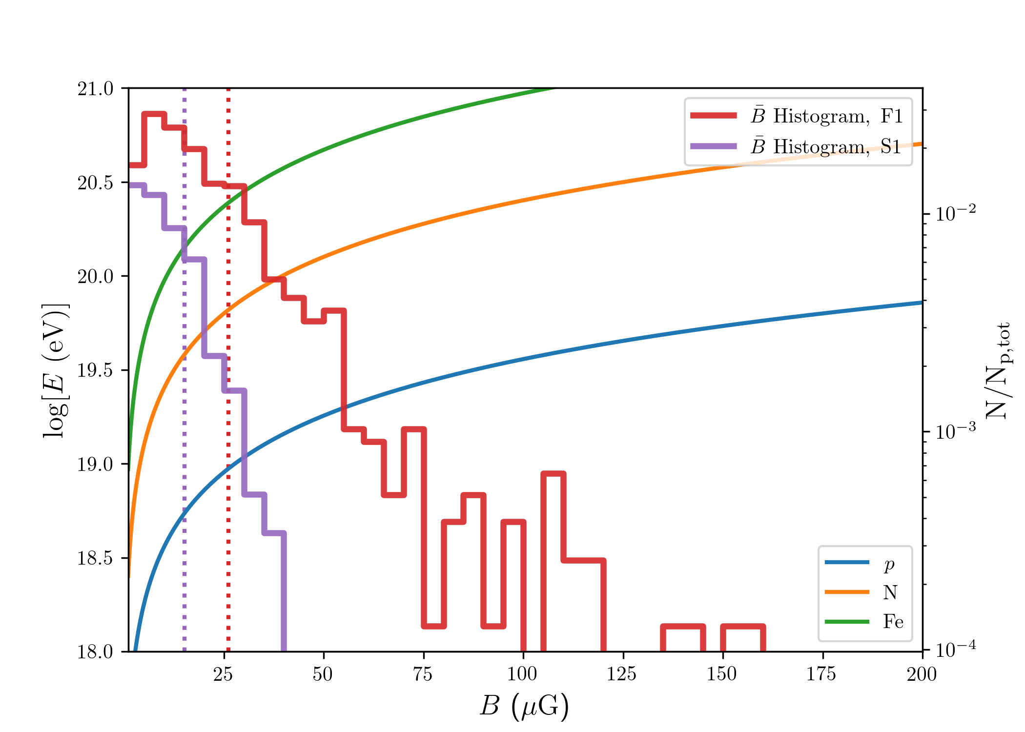
Figure 13: Maximum (Hillas) energy of protons, N and Fe for different values of $B$ (blue, orange and green curves) and for our chosen representative shock parameters of $v_{s}=0.2c$ and $r_{s}=2$ kpc. The red histogram shows the distribution of $\bar{B}$ from equation 18 for the strongest shocks that each tracer particle passes through in the F1 and S1 simulations, while the dotted lines show the mean values.

In Fig. 13 we show curves of the Hillas energy for $r_{s}=2$kpc, $v_{s}=0.2c$ for protons ($Z=1$, blue-solid line), He nuclei ($Z=2$, orange-solid line), and Fe nuclei ($Z=26$, green-solid line) as a function of the magnetic field. Overplotted is the distribution of $\bar{B}$ for the strongest shocks that each tracer particle passes through in the F1 and S1 simulations simulation, while the dotted lines show the mean values of these histograms ($15.18\mu$G and $26.95\mu$G). For $B=26.95\mu$G, $v_{s}=0.2c$ and $r_{s}=2$kpc, the Hillas energy is $9.70\times 10^{18}$eV, while for the strongest magnetic fields ($\approx 140\mu$G) the Hillas energy is $5.04\times 10^{19}$eV.

6.4 Scalability

The quoted values for $\bar{B}$ and $E_{H}$ are for a specific simulation, but will scale with the physical parameters. The magnetic field confining the CRs should be proportional to $\sqrt{\rho_{j}v_{j}^{2}}$ (Bell et al., 2013), while the characteristic sizes in the system will scale with jet width, $r_{j}$, provided that the value of $r_{c}$ is also scaled accordingly with $r_{j}$. If the most efficient acceleration to high energy always occurs at some critical shock velocity then we should expect $E_{\mathrm{max}}\propto\sqrt{\rho_{j}v_{j}^{2}}r_{j}$, that is, the maximum energy should be proportional to the square root of the jet power, although in reality the scaling is likely to be more complex. The jet powers we have adopted are in the FRII range but dramatically lower than estimates for the kinetic jet power in Cygnus A, for example ($\sim 10^{46}$ erg s^-1; Wilson et al., 2006; Ito et al., 2007; Kino & Kawakatu, 2005), implying that maximum CR energies can be higher in certain sources. If non- or mildly relativistic shocks in backflows are indeed ubiquitous then the limiting factor on the CR energy is probably the jet power. Given this expectation, we discuss some general jet power requirements with reference to both the observed radio galaxy luminosity function and the kinetic power to radiative luminosity relationship in the next section.

6.5 Other types of shock

In our analysis, we have focused on shocks in the lobes of radio galaxies, which are primarily produced in the supersonic backflows that form near the jet hotspot. It is interesting to consider whether the bow shock, reconfinement shocks, or termination shocks may prove to be good UHECR accelerators. The strongest shock in the jet-lobe system is typically the termination shock, but this is expected to be relativistic (e.g. Begelman et al., 1984) and thus a poor accelerator to EeV energies (Lemoine & Pelletier, 2010; Reville & Bell, 2014; Bell et al., 2018). It is possible that the termination shock velocity is not highly relativistic, in which case termination shocks may still be able to accelerate UHECRs, especially since the critical velocity below which acceleration to high energy becomes efficient is not yet clear. However, observations of radio galaxy hotspots suggest that jet termination shocks cannot accelerate particles to EeV energies (Araudo et al., 2016, 2018). Jet reconfinement shocks have similar difficulties, since they are also generally relativistic and their oblique geometry lowers the energy gain per shock crossing (e.g. Meli & Biermann, 2013). The complex interaction between the jet and the cocoon does produce some extended shock features, some of which will be included in the criteria for our shock detection as described in section 5. These structures merit future investigation but at face value appear less attractive UHECR accelerators than the shocks in backflows.

The bow shock may also accelerate particles, but the shock velocity is low – approximately equal to the jet advance speed ($\sim c/100$) at the tip of the bow shock and lower by a geometric factor away from the jet head. The bow shock smoothly transitions into a sound wave for the slowest advance speeds or high external pressures, as can be seen in Fig. 7. The magnetic field is also lower in the bow shock than in the jet or lobe as it is just a compressed version of the ambient field, while amplification is likely inefficient on UHECR Larmor radius scales. These factors may partly account for the absence of synchrotron emission from radio galaxy bow shocks (Carilli et al., 1988), although synchrotron X-ray emission can be detected in Centaurus A’s bow shock, where the maximum particle energy is thought to be well below the UHECR regime (Croston et al., 2009). The bow shock in radio galaxies is likely a poor accelerator of UHECRs.

7 Discussion

We have demonstrated that FRII-like jets produce the right kind of shocks to accelerate CRs to rigidities above $10$EV, but this is not the only requirement for a successful model for UHECR production. We therefore discuss constraints on the power, isotropy, proximity and composition requirements for UHECR sources, informed by results from UHECR detectors and radio surveys and our recent discussion of UHECR anisotropies (Matthews et al., 2018). In this discussion, attenuation due to the GZK effect (Greisen, 1966; Zatsepin & Kuz’min, 1966) and photodisintegration (Stecker & Salamon, 1999) is important as it sets the characteristic maximum distance a high-energy proton or nucleus can travel. The horizon distance is strongly energy and composition dependent, but is typically on the order of $100$Mpc (e.g. Alves Batista et al., 2016; Wykes et al., 2017). We adopt this as a canonical value but note the wide variation in attenuation lengths for different species and at different CR energies.

7.1 Are there enough powerful sources?

At least two basic energetic requirements must be satisfied by an UHECR source. The first is the minimum power constraint, described in various contexts by a number of authors (Lovelace, 1976; Waxman, 1995, 2001; Blandford, 2000; Massaglia, 2009). For acceleration to a given rigidity, this constraint requires that sufficient power passes through the shock for the magnetic field to reach ${\cal R}/(v_{s}r_{s})$. In the case of particle acceleration at shocks this can be computed by considering the magnetic energy density $U_{\mathrm{mag}}=B^{2}/(2\mu_{0})$ and the Hillas energy (equation 1). Since the maximum magnetic power delivered through a shock of size $r_{s}$ is approximately $U_{\mathrm{mag}}v_{s}r_{s}^{2}$, we can write an equation, independent of $B$, for the minimum power $Q_{\mathrm{min}}$, given by

$$Q_{\mathrm{min}}=f_{s}~{}\frac{{\cal R}^{2}}{2\mu_{0}v_{s}},$$ (19)

which is equivalent to

$$\left(\frac{Q_{\mathrm{min}}}{\rm erg\,s^{-1}}\right)\sim 10^{44}~{}\left(\frac{f_{s}}{0.1}\right)^{-1}~{}\left(\frac{v_{s}}{0.1c}\right)^{-1}~{}\left(\frac{{\cal R}}{10\,\rm EeV}\right)^{2}.$$ (20)

Here, $f_{s}$ is the fraction of the jet’s overall energy that is channeled through the right kind of shock for acceleration to high energy. We adopt $f_{s}=0.1$ based on the results from section 5.3.

The second energetic requirement for UHECR sources is that the observed number of UHECRs arriving at Earth can be produced. To calculate the luminosity in UHECRs that can be produced from a radio galaxy, we consider a jet of kinetic power $Q_{j}$, with some fraction $f_{s}$ of the jet power channelled through the right kind of shock for acceleration to high energy, and a further characteristic fraction, $\eta$ of each shock’s energy budget going into UHECRs above energy $E_{u}$. In reality, $f_{s}$ and $\eta$ take different values for different shocks and for different values of $E_{u}$; nonetheless, we can estimate characteristic values. The value of $\eta$ can be estimated by considering a differential particle number distribution proportional to $E^{-\beta}$ in the number of CRs such that the differential luminosity is $dL/dE\propto E^{1-\beta}$. If we adopt $E_{1}=1$ GeV ($\sim m_{p}c^{2}$) as the lower energy bound for the total CR luminosity and define $\eta_{0}=0.3$ as the fraction of the shock energy going into CRs at all energies then we obtain

$$\eta(E>E_{u})=\begin{cases}\eta_{0}\frac{\ln(E_{2}/E_{u})}{\ln(E_{2}/E_{1})}\approx 0.05,&\text{if}\ \beta=2,\\ \eta_{0}\frac{E_{2}^{-0.2}-E_{u}^{-0.2}}{E_{2}^{-0.2}-E_{1}^{-0.2}}\approx 0.003&\text{if}\ \beta=2.2,\\ \end{cases}$$ (21)

where $E_{2}=10^{20}$ eV is a maximum energy cutoff and for the spectral index we choose as representative examples $\beta=2.2$ as expected for the intrinsic Galactic CR spectrum (Gaisser et al., 1998; Hillas, 2005) and $\beta=2$ to match the theoretical expectation from DSA (Bell, 1978a). Clearly, the efficiency of UHECR production is strongly dependent on the CR spectral index and characteristics of the shock accelerating the CRs.

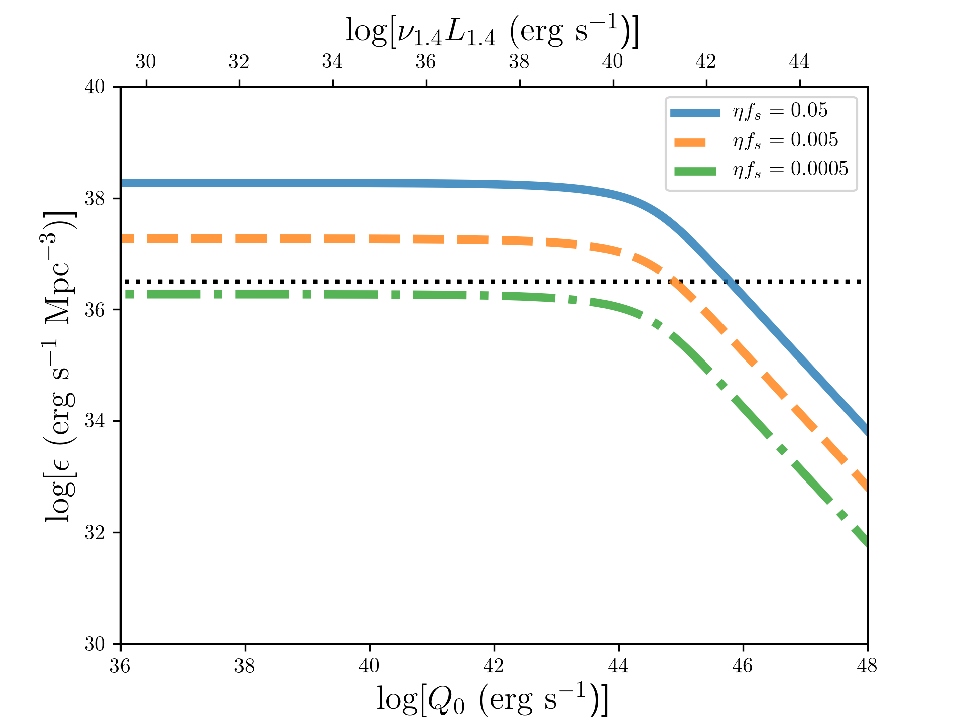
Figure 14: The UHECR luminosity density produced by a population of radio galaxies as a function of the lower limit on the integral over jet power in equation 23, $Q_{0}$. The horizontal line shows the approximate observed UHECR luminosity density above $10^{18}$ eV observed at Earth.

Jet power is related to the observed radio luminosity of a system; for the purposes of this estimate we adopt equation 1 from Cavagnolo et al. (2010), which can be written as

$$\left(\frac{Q_{j}(L_{1.4})}{\mathrm{erg~{}s^{-1}}}\right)=10^{0.75\log(\nu_{1.4}~{}L_{1.4})+13.91}$$ (22)

where $L_{1.4}$ is the monochromatic radio luminosity at $1.4$ GHz in erg s^-1 Hz^-1. For a given 1.4 GHz luminosity function $\phi$ in units of Mpc${}^{-3}\log(L_{1.4})^{-1}$, the luminosity density in UHECRs is

$$\left(\frac{\epsilon_{u}}{\mathrm{erg~{}s}^{-1}~{}\mathrm{Mpc}^{-3}}\right)=f_{s}\eta\int^{\infty}_{Q_{\mathrm{0}}}Q_{j}(L_{1.4})~{}\phi~{}d(\log L_{1.4})$$ (23)

We adopt the double power law luminosity function for radio galaxies given by Heckman & Best (2014, eq. 7) with a break at $10^{31.95}$ erg s^-1 Hz^-1 and plot $\epsilon_{u}$ as a function of $Q_{\mathrm{0}}$ in Fig. 14, for some representative values of $\eta~{}f_{s}$. Comparing to the dotted line, which shows the the UHECR luminosity density (luminosity per unit volume) above $10^{18}$eV reported by Nizamov & Pshirkov (2018) of $\epsilon_{18}=10^{44}$erg yr^-1 Mpc^-3, the figure makes it clear that, within the approximate spirit of the calculation, powerful radio galaxies are common enough to produce the observed UHECR fluxes at Earth. However, when we consider acceleration to $\sim 60$EeV and beyond the additional constraint of the GZK/photodistintegration horizon is important. As shown by a number of authors (e.g. Blandford, 2000; Massaglia, 2007a; Eichmann et al., 2018; Matthews et al., 2018), powerful radio galaxies within $\sim 100$ Mpc are scarce.

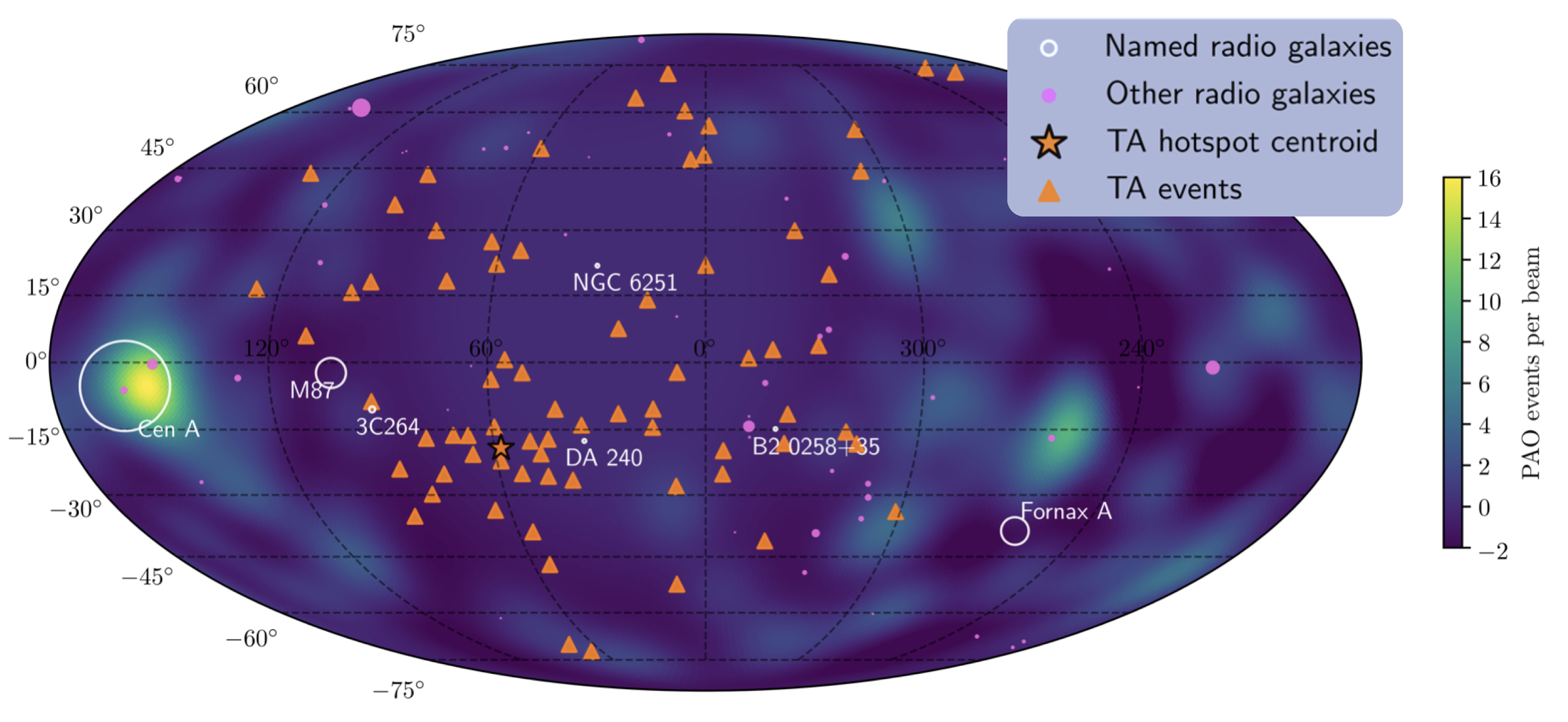
Figure 15: A Mollweide projection in supergalactic coordinates showing a colormap of the PAO events per beam above $60$EeV, with the TA event ($>57$EeV) arrival directions overlaid (orange triangles) and the TA hotspot centroid from Abbasi et al. (2014) marked with a star. The circles show all radio galaxies from the vV12 catalogue with distances $<150$ Mpc and with radio luminosities $\nu L_{\nu}>2\times 10^{40}$ erg s^-1 at 1.4 GHz, with the size of the circles proportional to the observed flux density. The white circles are specifically discussed in the text; otherwise the circles are colour pink.

7.2 UHECRs from dormant lobes inflated by powerful jets?

In Matthews et al. (2018), we showed that the excesses above isotropy in the PAO data (Pierre Auger Collaboration et al., 2018) may be explained by considering strong UHECR contributions from Centaurus A and Fornax A. Both these sources show giant lobes whose total energy contents are large compared to the energy input from the currently active jet in the system. There is also evidence of declining AGN activity in Fornax A (Iyomoto et al., 1998; Lanz et al., 2010) and of recent merger activity in both sources (Mackie & Fabbiano, 1998; Horellou et al., 2001). Together, these considerations led us to invoke a scenario in which Fornax A and Centaurus A had both had more powerful, possibly FRII-like, jet “outburst” in the past, during which UHECRs were accelerated, meaning that their giant lobes now act as (slowly leaking) UHECR reservoirs.

The observed UHECR excess map above $60$ EeV from Pierre Auger Collaboration et al. (2018) in supergalactic coordinates is shown as a Mollweide projection in Fig. 15. The two “hotspots” discussed by Matthews et al. (2018) can be seen close to Fornax A and Centaurus A. The TA events above $57$ EeV from Abbasi et al. (2014) are overlaid on the plot, together with the positions of all radio galaxies from the van Velzen et al. (2012) catalogue that are within 150 Mpc of Earth and have radio luminosities $\nu L_{\nu}>2\times 10^{40}$ erg s^-1 at 1.4 GHz. This luminosity cutoff corresponds to a minimum kinetic power of approximately $10^{44}$ erg s^-1 (see equation 22). The radio galaxies discussed in this paper are labelled.

The TA arrival directions have an excess just below the supergalactic plane, often referred to as the TA hotspot, with a characteristic spread of $\sim 20^{\circ}$ (Abbasi et al., 2014). It is possible that the TA events are dominated by a fairly diffuse component along the supergalactic plane, whereas the PAO events could instead be dominated by a few nearby radio galaxies in the southern sky. It might also be possible to explain the TA hotspot by an association with individual radio galaxies. The radio galaxy NGC 6251 is intriguingly similar to Centaurus A and Fornax A in that it has extremely large lobes (linear extent $2$ Mpc) with large total energy contents (Waggett et al., 1977) and is thought to be an extended $\gamma$-ray source (Takeuchi et al., 2012). Similarly, the restarted radio galaxy B2 0258$+$35 (hosted by NGC 1167 Shulevski et al., 2012; Brienza et al., 2018) has giant lobes $\sim 240$ kpc across, and shows evidence for past/ongoing merger activity (Emonts et al., 2010; Struve et al., 2010), which may have triggered a powerful past jet episode (Shulevski et al., 2012). The offsets from the TA hotspots for NGC 6251 and B2 0258$+$35 are $48.7^{\circ}$ and $73.8^{\circ}$, respectively. Thus, the required magnetic deflections are large, but $48.7^{\circ}$ is possible for an ${\cal R}\sim 10$EV CR from a source at NGC 6251’s position and distance in either the Galactic magnetic field (Farrar, 2016, see their figure 2) or an extragalactic field of $\sim 1$nG in accordance with results from (Bray & Scaife, 2018). Other sources such as DA 240 and 3C 264 are also interesting candidates. It is difficult to draw more robust conclusions about arrival directions without detailed modelling that takes into account attenuation losses and magnetic field deflections, which are both highly composition-dependent (e.g. alves_batista_cosmic_2016; Wykes et al., 2017); nevertheless, an association of UHECR arrival directions with giant-lobed radio galaxies is at least feasible.

While a “dormant source” scenario was invoked by Matthews et al. (2018) to explain UHECR arrival directions, it is also appealing in terms of source energetics. The minimum power requirement (equation 20) and minimum source densities (Fig. 14) provide quite strict limits for UHECR acceleration in steady sources. These limits initially appear problematic when we consider the relative scarcity of nearby (within a GZK radius) FRII/high-power sources (e.g. Massaglia, 2007a, b; van Velzen et al., 2012; Matthews et al., 2018). As pointed out by, e.g., Nizamov & Pshirkov (2018), the former constraint is alleviated by allowing for variable sources. In such a situation, the power requirement is no longer instantaneous and instead we require a powerful outburst satisfying $Q>Q_{\mathrm{min}}$ within the shorter of the GZK time ($\sim 300$ Myr) or UHECR escape time. The constraints from Fig. 14 are unchanged, as it is the active source density that matters; we do not necessarily require any sources to be currently active within a characteristic GZK radius, but we require that sources are on average active enough to produce the observed UHECR flux at Earth.

The arguments made so far in this section are not specific to exactly where the UHECRs are accelerated in the source, as they only require that there is sufficient power in the jet. If the UHECRs are accelerated in backflows then that imposes an additional limit, in that the physical conditions for backflow must have been met during an outburst phase. Backflows are not confined to FRIIs. The existence of backflows has been inferred in two lobed FRI sources with radio luminosities of $\approx 10^{41}$erg s^-1 (Laing & Bridle, 2012), while the FRI-FRII luminosity break is slightly higher, at approximately $4\times 10^{41}$erg s^-1 (Fanaroff & Riley, 1974). Neither of these thresholds should be thought of as a clearly delineated boundary, but they allow us to estimate if sources with strong backflows might be common enough to explain the observed UHECRs at Earth. Comparing the expected UHECR luminosity density from sources above these luminosities to the observed UHECR luminosity density (Fig. 14) suggests that a hypothesis in which UHECRs originate in FRII or high power, lobed-FRI radio galaxies is plausible.

8 Summary & Conclusions

We have used hydrodynamic simulations of AGN jets together with some general physical arguments to show that backflowing streams present in radio galaxy lobes should produce moderately strong shocks that can accelerate CRs to ultra-high energies. We summarise our work as follows:

• We have presented hydrodynamic simulations showing that strong backflows are expected in the lobes of radio galaxies and multiple shocks can occur along the backflow. A Bernoulli-like analysis applied to a streamline of steady flow helps elucidate many of the key physical effects, showing that the backflow should be thin and supersonic, with its velocity a significant fraction ($\sim 1/2$) of the jet velocity. The Mach number in the backflow increases as the pressure drops so as to equilibriate with the surrounding pressure in the cocoon. Backflows are generaly strongest for high density contrasts, wide lobes and powerful jets and are not confined to our fiducial parameter space.

• Our 3D simulations show similar overall behaviour to 2D cylindrical simulations in terms of backflow strength, but the breaking of azimuthal symmetry allows the kinetic energy to be focused into a stream of smaller cross-sectional area than when assuming a cylindrical geometry.

• We have used a combination of Lagrangian (tracer particles) and Eulerian (grid properties) techniques to analyse the shocks in our simulations. These methods reveal characteristic shock sizes of $r_{s}\sim 2$ kpc and shock velocities of $v_{s}\sim 0.2c$. Approximately $10\%$ of tracer particles pass through a shock of $M\gtrsim 3$. For a magnetic field of $140~{}\mu G$ this leads to a Hillas energy for protons of $5\times 10^{19}$eV (or equivalently, maximum rigidities of ${\cal R}\sim 50$EV).

• We have shown that the shocks that form in backflows have a number of key advantages over the relativistic jet termination shock for UHECR acceleration (see section 6.1). The shock velocities inevitably cover a range of values, meaning that many of the problems with DSA at relativistic shocks (e.g. Reville & Bell, 2014; Bell et al., 2018) can be avoided. Multiple shocks in the flow also allow for multiple opportunities for acceleration via DSA and magnetic field amplification at the shock. Perhaps even more importantly, multiple shocks along a flow mean that there is more than one way for the magnetic field to be amplified and, crucially, the amplification timescale at the shock is not necessarily the limiting factor for acceleration to high energy. As a result, the Hillas energy can be expected to act as a better estimate of the maximum CR energy in jet backflows than in the case of supernova remnants where the energy is lower than Hillas by a significant factor (e.g. Bell et al., 2013).

• We have used radio galaxy luminosity functions and empirical radio to jet power relationships to show that radio jets are, on average, common and powerful enough to produce the UHECR flux arriving at Earth. However, there are not enough steady powerful sources within a canonical GZK horizon to produce the observed UHECRs. We have therefore expanded on the ideas presented by Matthews et al. (2018), exploring the possibility that UHECRs are produced during powerful past jet episodes and are now slowly escaping from “dormant” giant radio sources, such as Fornax A, Centaurus A and NGC 6251. This class of dormant sources may be able to explain the observed anisotropies from the PAO and TA UHECR observatories.

While the scenario we have presented here offers good overall prospects as an UHECR production model, we note that many of the requirements for UHECR acceleration may be met in other situations other than backflows. Fundamentally, regardless of the class of astrophysical system considered, one has to engineer a “goldilocks” situation where a large amount of power ($\sim 10^{44}$ erg s^-1) is channeled through a strong shock meeting the Hillas criterion, without the shock velocity becoming too large. Shocks in the backflows of radio galaxies provide one way to do this.

References

- Abbasi et al. (2014) Abbasi R. U., et al., 2014, ApJ, 790, L21
- Abbasi et al. (2015) Abbasi R. U., et al., 2015, Astropart. Phys., 64, 49
- Abreu et al. (2010) Abreu P., et al., 2010, Astropart. Phys., 34, 314
- Abu-Zayyad et al. (2013) Abu-Zayyad T., et al., 2013, ApJ, 777, 88
- Achterberg (1990) Achterberg A., 1990, A&A, 231, 251
- Alves Batista et al. (2016) Alves Batista R., et al., 2016, J. Cosmology Astropart. Phys., 05, 038
- Amato & Blasi (2009) Amato E., Blasi P., 2009, MNRAS, 392, 1591
- Appl & Camenzind (1988) Appl S., Camenzind M., 1988, A&A, 206, 258
- Appl et al. (2000) Appl S., Lery T., Baty H., 2000, A&A, 355, 818
- Araudo et al. (2015) Araudo A. T., Bell A. R., Blundell K. M., 2015, ApJ, 806, 243
- Araudo et al. (2016) Araudo A. T., Bell A. R., Crilly A., Blundell K. M., 2016, MNRAS, 460, 3554
- Araudo et al. (2018) Araudo A. T., Bell A. R., Blundell K. M., Matthews J. H., 2018, MNRAS, 473, 3500
- Armstrong et al. (1985) Armstrong T. P., Pesses M. E., Decker R. B., 1985, Washington DC American Geophysical Union Geophysical Monograph Series, 35, 271
- Axford et al. (1977) Axford W. I., Leer E., Skadron G., 1977, International Cosmic Ray Conference, 11, 132
- Begelman et al. (1984) Begelman M. C., Blandford R. D., Rees M. J., 1984, Rev. Mod. Phys., 56, 255
- Bell (1978a) Bell A. R., 1978a, MNRAS, 182, 147
- Bell (1978b) Bell A. R., 1978b, MNRAS, 182, 443
- Bell (2004) Bell A. R., 2004, MNRAS, 353, 550
- Bell (2005) Bell A. R., 2005, MNRAS, 358, 181
- Bell (2014) Bell A. R., 2014, Brazilian Journal of Physics, 44, 415
- Bell et al. (2013) Bell A. R., Schure K. M., Reville B., Giacinti G., 2013, MNRAS, 431, 415
- Bell et al. (2018) Bell A. R., Araudo A. T., Matthews J. H., Blundell K. M., 2018, MNRAS, 473, 2364
- Beskin et al. (2011) Beskin V. S., Kovalev Y. Y., Nokhrina E. E., 2011, preprint, (arXiv:1107.0565)
- Blandford (2000) Blandford R. D., 2000, Phys. Scr., 85, 191
- Blandford & Eichler (1987) Blandford R., Eichler D., 1987, Physics Reports, 154, 1
- Blandford & Ostriker (1978) Blandford R. D., Ostriker J. P., 1978, ApJ, 221, L29
- Blandford & Ostriker (1980) Blandford R. D., Ostriker J. P., 1980, ApJ, 237, 793
- Blundell et al. (1999) Blundell K. M., Rawlings S., Willott C. J., 1999, AJ, 117, 677
- Bray & Scaife (2018) Bray J. D., Scaife A. M. M., 2018, ApJ, 861, 3
- Brienza et al. (2018) Brienza M., et al., 2018, preprint, 1807, arXiv:1807.07280
- Burgess (1987) Burgess D., 1987, J. Geophys. Res., 92, 1119
- Caprioli (2015) Caprioli D., 2015, ApJ, 811, L38
- Carilli & Barthel (1996) Carilli C. L., Barthel P. D., 1996, A&AReview, 7, 1
- Carilli et al. (1988) Carilli C. L., Perley R. A., Dreher J. H., 1988, ApJ, 334, L73
- Cassam-Chenaï et al. (2007) Cassam-Chenaï G., Hughes J. P., Ballet J., Decourchelle A., 2007, ApJ, 665, 315
- Cavagnolo et al. (2010) Cavagnolo K. W., McNamara B. R., Nulsen P. E. J., Carilli C. L., Jones C., Bîrzan L., 2010, ApJ, 720, 1066
- Childs et al. (2005) Childs H., Brugger E. S., Bonnell K. S., Meredith J. S., Miller M., Whitlock B. J., Max N., 2005, in Proceedings of IEEE Visualization 2005. pp 190–198
- Cielo et al. (2014) Cielo S., Antonuccio-Delogu V., Macciò A. V., Romeo A. D., Silk J., 2014, MNRAS, 439, 2903
- Clarke et al. (1986) Clarke D. A., Norman M. L., Burns J. O., 1986, ApJ, 311, L63
- Croston et al. (2009) Croston J. H., et al., 2009, MNRAS, 395, 1999
- De Young (2001) De Young D. S., 2001. p. 75, http://adsabs.harvard.edu/abs/2001ASPC..250...75D
- De Young (2002) De Young D. S., 2002, New Astronomy Reviews, 46, 393
- Decker (1988) Decker R. B., 1988, ApJ, 324, 566
- Eichmann et al. (2018) Eichmann B., Rachen J. P., Merten L., van Vliet A., Becker Tjus J., 2018, J. Cosmology Astropart. Phys., 02, 036
- Emonts et al. (2010) Emonts B. H. C., et al., 2010, MNRAS, 406, 987
- English et al. (2016) English W., Hardcastle M. J., Krause M. G. H., 2016, MNRAS, 461, 2025
- Ester et al. (1996) Ester M., Kriegel H.-P., Sander J., Xu X., 1996, in Proceedings of the Second International Conference on Knowledge Discovery and Data Mining. KDD’96. AAAI Press, Portland, Oregon, pp 226–231, http://dl.acm.org/citation.cfm?id=3001460.3001507
- Falle (1991) Falle S. A. E. G., 1991, MNRAS, 250, 581
- Fanaroff & Riley (1974) Fanaroff B. L., Riley J. M., 1974, MNRAS, 167, 31P
- Farrar (2016) Farrar G. R., 2016, IAU Focus Meeting, 29B, 723
- Fermi (1949) Fermi E., 1949, Physical Review, 75, 1169
- Gaibler et al. (2009) Gaibler V., Krause M., Camenzind M., 2009, MNRAS, 400, 1785
- Gaisser et al. (1998) Gaisser T. K., Protheroe R. J., Stanev T., 1998, ApJ, 492, 219
- Giacalone & Jokipii (2007) Giacalone J., Jokipii J. R., 2007, ApJ, 663, L41
- Giannios & Spruit (2006) Giannios D., Spruit H. C., 2006, A&A, 450, 887
- Gieseler & Jones (2000) Gieseler U. D. J., Jones T. W., 2000, A&A, 357, 1133
- Greisen (1966) Greisen K., 1966, Phys. Rev. Lett., 16, 748
- Hardcastle (2010) Hardcastle M. J., 2010, MNRAS, 405, 2810
- Hardcastle & Croston (2005) Hardcastle M. J., Croston J. H., 2005, MNRAS, 363, 649
- Hardcastle & Krause (2013) Hardcastle M. J., Krause M. G. H., 2013, MNRAS, 430, 174
- Hardcastle & Krause (2014) Hardcastle M. J., Krause M. G. H., 2014, MNRAS, 443, 1482
- Haswell et al. (1992) Haswell C. A., Tajima T., Sakai J.-I., 1992, ApJ, 401, 495
- Heckman & Best (2014) Heckman T. M., Best P. N., 2014, Annual Review of A&A, 52, 589
- Hillas (1984) Hillas A. M., 1984, ARA&A, 22, 425
- Hillas (2005) Hillas A. M., 2005, Journal of Physics G Nuclear Physics, 31, R95
- Horellou et al. (2001) Horellou C., Black J. H., van Gorkom J. H., Combes F., van der Hulst J. M., Charmandaris V., 2001, A&A, 376, 837
- Hunter (2007) Hunter J. D., 2007, Computing In Science & Engineering, 9, 90
- Ineson et al. (2013) Ineson J., Croston J. H., Hardcastle M. J., Kraft R. P., Evans D. A., Jarvis M., 2013, ApJ, 770, 136
- Ineson et al. (2015) Ineson J., Croston J. H., Hardcastle M. J., Kraft R. P., Evans D. A., Jarvis M., 2015, MNRAS, 453, 2682
- Ineson et al. (2017) Ineson J., Croston J. H., Hardcastle M. J., Mingo B., 2017, MNRAS, 467, 1586
- Ito et al. (2007) Ito H., Kino M., Kawakatu N., Isobe N., Yamada S., 2007, Astrophysics and Space Science, 311, 335
- Iyomoto et al. (1998) Iyomoto N., Makishima K., Tashiro M., Inoue S., Kaneda H., Matsumoto Y., Mizuno T., 1998, ApJ, 503, L31
- Kaiser & Alexander (1997) Kaiser C. R., Alexander P., 1997, MNRAS, 286, 215
- Keppens et al. (2008) Keppens R., Meliani Z., van der Holst B., Casse F., 2008, A&A, 486, 663
- King (1972) King I. R., 1972, ApJ, 174, L123
- Kino & Kawakatu (2005) Kino M., Kawakatu N., 2005, MNRAS, 364, 659
- Kirk & Reville (2010) Kirk J. G., Reville B., 2010, ApJ, 710, L16
- Koessl & Mueller (1988) Koessl D., Mueller E., 1988, A&A, 206, 204
- Komissarov (1999) Komissarov S. S., 1999, MNRAS, 308, 1069
- Koyama et al. (1995) Koyama K., Petre R., Gotthelf E. V., Hwang U., Matsuura M., Ozaki M., Holt S. S., 1995, Nature, 378, 255
- Krause (2005) Krause M., 2005, A&A, 431, 45
- Krymskii (1977) Krymskii G. F., 1977, Soviet Physics Doklady, 22, 327
- Kulsrud & Pearce (1969) Kulsrud R., Pearce W. P., 1969, ApJ, 156, 445
- Lagage & Cesarsky (1983) Lagage P. O., Cesarsky C. J., 1983, A&A, 118, 223
- Laing (1989) Laing R., 1989. pp 27–43, doi:10.1007/BFb0036010, http://adsabs.harvard.edu/abs/1989LNP...327...27L
- Laing & Bridle (2012) Laing R. A., Bridle A. H., 2012, MNRAS, 424, 1149
- Lanz et al. (2010) Lanz L., Jones C., Forman W. R., Ashby M. L. N., Kraft R., Hickox R. C., 2010, ApJ, 721, 1702
- Leismann et al. (2005) Leismann T., Antón L., Aloy M. A., Müller E., Martí J. M., Miralles J. A., Ibáñez J. M., 2005, A&A, 436, 503
- Lemoine & Pelletier (2010) Lemoine M., Pelletier G., 2010, MNRAS, 402, 321
- Lerche (1967) Lerche I., 1967, ApJ, 147, 689
- Litvinenko (1996) Litvinenko Y. E., 1996, ApJ, 462, 997
- Lovelace (1976) Lovelace R. V. E., 1976, Nature, 262, 649
- Mackie & Fabbiano (1998) Mackie G., Fabbiano G., 1998, AJ, 115, 514
- Marcowith & Kirk (1999) Marcowith A., Kirk J. G., 1999, A&A, 347, 391
- Marti et al. (1997) Marti J. M., Müller E., Font J. A., Ibáñez J. M. Z., Marquina A., 1997, ApJ, 479, 151
- Massaglia (2007a) Massaglia S., 2007a, Nuclear Physics B Proceedings Supplements, 165, 130
- Massaglia (2007b) Massaglia S., 2007b, Nuclear Physics B Proceedings Supplements, 168, 302
- Massaglia (2009) Massaglia S., 2009, Nuclear Physics B Proceedings Supplements, 190, 79
- Mathews (2014) Mathews W. G., 2014, ApJ, 783, 42
- Mathews & Guo (2012) Mathews W. G., Guo F., 2012, ApJ, 755, 13
- Matthews et al. (2017) Matthews J. H., Bell A. R., Blundell K. M., Araudo A. T., 2017, MNRAS, 469, 1849
- Matthews et al. (2018) Matthews J. H., Bell A. R., Blundell K. M., Araudo A. T., 2018, MNRAS, 479, L76
- Meli & Biermann (2013) Meli A., Biermann P. L., 2013, A&A, 556, A88
- Melrose & Crouch (1997) Melrose D., Crouch A., 1997, Publ. Astron. Soc. Australia, 14, 251
- Mendygral et al. (2012) Mendygral P. J., Jones T. W., Dolag K., 2012, ApJ, 750, 166
- Mignone et al. (2005) Mignone A., Plewa T., Bodo G., 2005, ApJS, 160, 199
- Mignone et al. (2007) Mignone A., Bodo G., Massaglia S., Matsakos T., Tesileanu O., Zanni C., Ferrari A., 2007, ApJS, 170, 228
- Milosavljević & Nakar (2006) Milosavljević M., Nakar E., 2006, ApJ, 651, 979
- Mueller et al. (1991) Mueller D., Swordy S. P., Meyer P., L’Heureux J., Grunsfeld J. M., 1991, ApJ, 374, 356
- Niemiec et al. (2008) Niemiec J., Pohl M., Stroman T., Nishikawa K.-I., 2008, ApJ, 684, 1174
- Nizamov & Pshirkov (2018) Nizamov B. A., Pshirkov M. S., 2018, preprint, (arXiv:1804.01064)
- Norman et al. (1982) Norman M. L., Winkler K.-H. A., Smarr L., Smith M. D., 1982, A&A, 113, 285
- Norman et al. (1995) Norman C. A., Melrose D. B., Achterberg A., 1995, ApJ, 454, 60
- O’Sullivan et al. (2009) O’Sullivan S., Reville B., Taylor A. M., 2009, MNRAS, 400, 248
- Pedregosa et al. (2011) Pedregosa F., et al., 2011, Journal of Machine Learning Research, 12, 2825
- Perley et al. (1984) Perley R. A., Dreher J. W., Cowan J. J., 1984, ApJ, 285, L35
- Pierre Auger Collaboration (2014) Pierre Auger Collaboration 2014, preprint, 1409, arXiv:1409.5083
- Pierre Auger Collaboration et al. (2007) Pierre Auger Collaboration et al., 2007, Science, 318, 938
- Pierre Auger Collaboration et al. (2008) Pierre Auger Collaboration et al., 2008, Astropart. Phys., 29, 188
- Pierre Auger Collaboration et al. (2017) Pierre Auger Collaboration et al., 2017, Science, 357, 1266
- Pierre Auger Collaboration et al. (2018) Pierre Auger Collaboration et al., 2018, preprint, 1801, arXiv:1801.06160
- Pope & Melrose (1994) Pope M. H., Melrose D. B., 1994, Proceedings of the Astronomical Society of Australia, 11, 175
- Reville & Bell (2014) Reville B., Bell A. R., 2014, MNRAS, 439, 2050
- Riquelme & Spitkovsky (2009) Riquelme M. A., Spitkovsky A., 2009, ApJ, 694, 626
- Riquelme & Spitkovsky (2010) Riquelme M. A., Spitkovsky A., 2010, ApJ, 717, 1054
- Saxton et al. (2002) Saxton C. J., Sutherland R. S., Bicknell G. V., Blanchet G. F., Wagner S. J., 2002, A&A, 393, 765
- Scheuer (1982) Scheuer P. A. G., 1982. pp 163–165, http://adsabs.harvard.edu/abs/1982IAUS...97..163S
- Scheuer (1995) Scheuer P. A. G., 1995, MNRAS, 277, 331
- Shulevski et al. (2012) Shulevski A., Morganti R., Oosterloo T., Struve C., 2012, A&A, 545, A91
- Sikora et al. (2005) Sikora M., Begelman M. C., Madejski G. M., Lasota J.-P., 2005, ApJ, 625, 72
- Skilling (1975a) Skilling J., 1975a, MNRAS, 172, 557
- Skilling (1975b) Skilling J., 1975b, MNRAS, 173, 245
- Skilling (1975c) Skilling J., 1975c, MNRAS, 173, 255
- Stecker & Salamon (1999) Stecker F. W., Salamon M. H., 1999, ApJ, 512, 521
- Stroman et al. (2009) Stroman T., Pohl M., Niemiec J., 2009, ApJ, 706, 38
- Struve et al. (2010) Struve C., Oosterloo T., Sancisi R., Morganti R., Emonts B. H. C., 2010, A&A, 523, A75
- Takeuchi et al. (2012) Takeuchi Y., et al., 2012, ApJ, 749, 66
- Tchekhovskoy & Bromberg (2016) Tchekhovskoy A., Bromberg O., 2016, MNRAS, 461, L46
- The Telescope Array Collaboration & The Pierre Auger Collaboration (2018) The Telescope Array Collaboration The Pierre Auger Collaboration 2018, preprint, (arXiv:1801.01018)
- Uchiyama et al. (2007) Uchiyama Y., Aharonian F. A., Tanaka T., Takahashi T., Maeda Y., 2007, Nature, 449, 576
- Völk et al. (2005) Völk H. J., Berezhko E. G., Ksenofontov L. T., 2005, A&A, 433, 229
- Waggett et al. (1977) Waggett P. C., Warner P. J., Baldwin J. E., 1977, MNRAS, 181, 465
- Waxman (1995) Waxman E., 1995, Phys. Rev. Lett., 75, 386
- Waxman (2001) Waxman E., 2001. eprint: arXiv:astro-ph/0103186, p. 122, http://adsabs.harvard.edu/abs/2001LNP...576..122W
- Wentzel (1974) Wentzel D. G., 1974, ARA&A, 12, 71
- Williams (1991) Williams A. G., 1991, in , Beams and Jets in Astrophysics. p. 342, http://adsabs.harvard.edu/abs/1991bja..book..342W
- Wilson et al. (2006) Wilson A. S., Smith D. A., Young A. J., 2006, ApJ, 644, L9
- Wykes et al. (2017) Wykes S., Taylor A. M., Bray J. D., Hardcastle M. J., Hillas M., 2017, preprint, 1706, arXiv:1706.08229
- Yang & Reynolds (2016) Yang H.-Y. K., Reynolds C. S., 2016, ApJ, 829, 90
- Zatsepin & Kuz’min (1966) Zatsepin G. T., Kuz’min V. A., 1966, Soviet Journal of Experimental and Theoretical Physics Letters, 4, 78
- Zdziarski et al. (2015) Zdziarski A. A., Sikora M., Pjanka P., Tchekhovskoy A., 2015, MNRAS, 451, 927
- Zirakashvili et al. (2008) Zirakashvili V. N., Ptuskin V. S., Völk H. J., 2008, ApJ, 678, 255
- de Souza (2017) de Souza V., 2017, preprint, (arXiv:1701.06812)
- van Velzen et al. (2012) van Velzen S., Falcke H., Schellart P., Nierstenhöfer N., Kampert K.-H., 2012, A&A, 544, A18