Analyzing Dynamic Ideological Communities in Congressional Voting Networks

Abstract

We here study the behavior of political party members aiming at identifying how ideological communities are created and evolve over time in diverse (fragmented and non-fragmented) party systems. Using public voting data of both Brazil and the US, we propose a methodology to identify and characterize ideological communities, their member polarization, and how such communities evolve over time, covering a 15-year period. Our results reveal very distinct patterns across the two case studies, in terms of both structural and dynamic properties.

1 Introduction

Party systems can be characterized based on their fragmentation and polarization [30]. Party fragmentation corresponds to the number of parties existing in a political system (e.g., a country) while polarization is related to the multiple opinions that lead to the division of members into groups with distinct political ideologies [30, 14]. In countries where the party system has a low fragmentation, the polarization of political parties can be seen more clearly since one party tends to occupy more seats supporting the government and the other opposes it [21]. On the other hand, in fragmented systems the multiple political parties often make use of coalitions, a type of inter-party alliance, to raise their relevance in the political system and reach a common end [2, 8]. Thus, a great amount of ideological similarity, as expressed by their voting decisions, is often observed across different parties.

Previous work has analyzed the behavior of political party members through the modeling of voting data in signed and weighted networks [3, 28, 25, 11, 10, 4, 19, 24]. These prior efforts tackled topics such as community detection, party cohesion and loyalty analysis, governance of a political party and member influence in such networks. However, the identification and characterization of ideological communities, particularly in fragmented party systems, require observing some issues, such as: (i) presidents define coalitions throughout government in order to strengthen the implementation of desired public policies, which may be ruptured after a period of time [20, 8]; (ii) political members have different levels of partisanship and loyalty, and their political preferences may change over time [5, 3]; and (iii) different political parties may have the same political ideology, being redundant under a party system [23].

In such context, we here study the behavior of political party members aiming at identifying how ideological communities are created and evolve over time. To that end, we consider two case studies, Brazil and US, which are representatives of distinct party systems: whereas the former is highly fragmented and redundant [23], the latter is not fragmented but rather polarized with two major parties, although some party members can be considered less polarized [25, 11]. Using public datasets of the voting records in the House of Representatives of both countries during a 15-year period, we characterize the emergence and evolution of communities of House members with similar political ideology (captured by their voting behavior) by using complex network concepts. Specifically, we tackle three research questions (RQs):

• RQ1: How do ideological communities are characterized in governments with different (i.e., fragmented and non-fragmented) party systems? We model the voting behavior of each House of Representatives during a given time period using a network, where nodes represent House members, and weighted edges are added if two members voted similarly. We use the Louvain algorithm [7] to detect communities in each network and characterize structural properties of such communities. Unlike prior community analysis in the political context, we compare the properties of these communities in fragmented and in non-fragmented party systems.

• RQ2: How can we identify polarization in the ideological communities? We use neighborhood overlap [13] to estimate the tie strength associated to each network edge, characterizing it as either strong or weak. This approach to estimate tie strength has been employed in several contexts [16, 18, 22, 37] and also in the political context [35]. However, these prior studies were not interested in analyzing and comparing distinct political systems, as we do here. We use strong ties to identify polarized communities in each analyzed network.

• RQ3: How do polarized communities evolve over time? We analyze how polarized communities evolve over the years of a government, characterizing how the membership of such communities change over time.

In sum, the key contributions of our work are: (i) a methodology to identify and analyze dynamic ideological communities and their polarization in party systems based on complex network concepts; and (ii) two case studies covering strikingly different party systems over a quite broad time period. Our study shows that in fragmented party systems, such as Brazil, although party redundancy exists, some ideological communities exist and may, indeed, be polarized. However, such polarized communities are highly dynamic, greatly changing their membership over consecutive years. In the US, on the other hand, despite the strong and temporally stable party polarization, there are members, within each party, that exhibit different levels of polarization.

The rest of this paper is organized as follows. Section 2 briefly discusses related work, whereas Section 3 describes our modeling methodology and case studies. We then present our main results, tackling RQ1-RQ3 in Sections 4-6. Conclusions and future work are offered in Section 7.

2 Related Work

Complex networks constitute a set of theoretical and analytical tools to describe and analyze phenomena related to interactions occurring in the real world [29]. Among the many properties of a network, the interactions between pairs of nodes can be used to define the strength of these links (or tie strength) [13]. Indeed, tie strength is a property that has been widely studied in several domains. For example, the tie strength between pairs of people was studied in the phone call and Short Message System (SMS) networks, where a higher frequency of SMS and longer call duration characterize stronger ties [37]. The different types of interactions between Facebook users have also been used to define tie strength on that system [18]. Similarly, tie strength was used to build geolocation models based on Twitter data and exploited in the prediction of user location [22].

In the political context, the study of political ideologies has been largely accomplished through the analysis of roll call votes networks. In a roll call votes network, the nodes represent people (e.g., congressmen), and two nodes are connected if they have voted similarly in one (or more) voting sessions. In [3], the authors studied the committee’s formation in the US House of Representatives using roll call votes networks, finding that there is a cooperation between the Democratic and Republican parties. Although the polarization in recent decades has been increasing, there are moderate members in both parties, who cooperate with each other. In the same direction, authors in [28] studied the committees and subcommittees of US House of Representatives exploiting the network connections that are built according to common membership. Analogously, the polarization in the US Senate was evaluated using a network defined by the similarity of Senators’ votes [25].

In [11], the authors studied the relations between members of the Italian parliament according to their voting behavior, analyzing the community structure with respect to political coalitions and government alliances over time. Similarly, the cohesiveness of members of the European Parliament was investigated through the analysis of network models combining roll call votes and Twitter data [10]. Other approaches study the behavior of political members modeling roll call votes using signed networks. However, this type of analysis is appropriate for modeling only polarized systems [4]. Signed networks have also been used to evaluate aspects related to political governance and political party behavior [19]. In addition, an algorithm was proposed to evaluate signed networks and a case study was conducted using a European Parliament network capturing voting similarities between members [24]. In [19], the roll call votes of the Brazilian House of Representative was modeled using signed networks. The results revealed inefficient coalitions with the government as parties that make such coalitions have members distributed in different ideological communities over time. Orthogonally, others have investigated the ideology of political members and users through profiles of social networks [1, 12, 34].

Unlike prior work, our focus here is on the characterization of ideological communities in diverse, i.e., both fragmented and non-fragmented, party systems. We also propose to use tie strength, computed based on neighborhood overlap, to identify polarized communities under the party systems diversities, evaluating their evolution over time, on both party systems.

3 Methodology

In this section, we describe the methodology used in our study. We start by presenting basic concepts (Section 3.1) followed by our case studies (Section 3.2), and then describe our modeling of voting behavior (Section 3.3).

3.1 Basic Concepts

The House of Representatives is composed of several members who occupy the seats during each government period. House members participate in a series of voting sessions, when bills, amendments, and propositions are discussed and voted. Thus, attending such sessions is the most direct way for members to express their ideologies and positioning. When these members are associated with a large number of political parties, the party system in question is regarded as fragmented. In this case, during a term of office, coalition governments are established, leading political parties to organize themselves into ideological communities, defending together common interests during voting sessions [20, 30].

One can evaluate the behavior of parties and their members in terms of how cohesive they are as an ideological community by analyzing voting data using widely disseminated metrics, such as Rice’s Index. However, the use of Rice Index has been shown to be problematic when there are more than two voting options (other than only yes and no) [17], as is the case, for example, in the European Parliament and in our study, as we will see later.

Instead, we here employ the Partisan Discipline and Party Discipline metrics [23]. The former captures the ideological alignment of a member to her party (estimated by the behavior of the majority), and the latter expresses the ideological cohesiveness of a party. Given a member $m$, belonging to party $p_{m}$, the Partisan Discipline of $m$, $pd_{m}$ is given by the fraction of all voting sessions to which $m$ attended and voted similarly to the majority of $p_{m}$’s members. That is, let $n$ be the number of voting sessions attended by member $m$ and $I(m,p_{m},i)$ be 1 if member $m$ voted similarly to the majority of members of $p_{m}$ in voting session $i$ ($i=1..n$) and 0 otherwise. Then:

$$pd_{m}=\frac{\sum_{i=1}^{n}I(m,p_{m},i)}{n}$$ (1)

The Partisan Discipline can be generalized to assess the discipline and ideological alignment of a member to any community (not only his original party).

The Party Discipline of a party $p$ is computed as the average Partisan Discipline of all of its members, that is, $PD(p)=\frac{\sum_{m=1}^{M}pd_{m}}{M}$, where $M$ is the number of members of $p$. Party Discipline captures how cohesive a party (or community) is in a set of votes. Both metrics range from 0 to 1, where 1 indicates that a member or party is totally disciplined (or cohesive) and 0 otherwise.

3.2 Case Studies

We consider two case studies: Brazil and US. In Brazil, the House of Representatives consists of 513 seats. A member vote can be either Yes, No, Obstruction or Absence in each voting session. A Yes or No vote expresses, respectively, an agreement or disagreement with the given proposition. Both Absence and Obstruction mean that the member did not participate in the voting, although an Obstruction expresses the intention of the member to cause the voting session to be cancelled due to insufficient quorum. Similarly, the US House of Representatives includes 435 seats, and a member vote can be Yes, No or Not Voting, whereas the last one indicates the member was not present in the voting session. In our study, we disregard Absence and Not Voting votes, as they do not reflect any particular inclination of the members with respect to the topic under consideration. However, we do include Obstructions as they reflect an intentional action of the members and a clear opposition to the topic. Thus, for Brazil, three different voting options were considered.

For both case studies, we collected voting data from public sources. The plenary roll call votes of Brazil’s House of Representatives are available through an application programming interface (API) maintained by the government. We collected roll call votes between the $52^{th}$ and $55^{th}$ legislatures, from 2003 to 2017. US voting data covering the same 15-year period (i.e., between the $108^{th}$ and $115^{th}$ congresses) was collected through the ProPublica API. Each dataset consists of a sequence of the voting session; for each session, the dataset includes date, time and voting option of each participating member.

Table 1: Overview of our datasets.

Brazil
Leg.	Year	President (Party)	# of Voting Sessions	# of Votes	# of Parties	# of Members	Avg. PD	SD PD
$52^{th}$	2003	Lula (PT)	150	106755	23	435	88.23%	0.08
	2004	Lula (PT)	118	71576	23	377	87.43%	0.08
	2005	Lula (PT)	81	50616	24	382	88.91%	0.07
	2006	Lula (PT)	87	62358	24	419	91.12%	0.05
$53^{th}$	2007	Lula (PT)	221	190424	31	478	92.45%	0.07
	2008	Lula (PT)	157	122482	31	452	92.34%	0.07
	2009	Lula (PT)	156	125759	30	465	91.87%	0.06
	2010	Lula (PT)	83	63255	29	452	92.46%	0.05
$54^{th}$	2011	Dilma (PT)	98	78662	29	481	89.34%	0.08
	2012	Dilma (PT)	79	60219	28	454	89.56%	0.05
	2013	Dilma (PT)	158	115751	29	451	88.70%	0.06
	2014	Dilma (PT)	87	66154	28	451	92.93%	0.04
$55^{th}$	2015	Dilma (PT)	273	231031	28	502	85.84%	0.06
	2016	Dilma (PT) Temer (PMDB)	218	156006	28	452	90.12%	0.05
	2017	Temer (PMDB)	230	159704	29	435	89.76%	0.08
United States
Cong.	Year	President (Party)	# of Voting Sessions	# of Votes	# of Parties	# of Members	Avg. PD	SD PD
$108^{th}$	2003	George W. Bush (R)	623	258867	3	432	95.76%	0.03
	2004	George W. Bush (R)	502	203557	3	427	95.11%	0.03
$109^{th}$	2005	George W. Bush (R)	637	264735	3	432	95.02%	0.03
	2006	George W. Bush (R)	511	210592	3	428	94.98%	0.04
$110^{th}$	2007	George W. Bush (R)	956	297957	2	414	92.23%	0.04
	2008	George W. Bush (R)	605	244734	2	426	92.73%	0.04
$111^{th}$	2009	Barack Obama (D)	929	385344	3	431	93.78%	0.02
	2010	Barack Obama (D)	631	253296	3	422	95.34%	0.01
$112^{th}$	2011	Barack Obama (D)	908	377601	2	428	91.98%	0.01
	2012	Barack Obama (D)	621	253812	2	425	91.50%	0.01
$113^{th}$	2013	Barack Obama (D)	594	245430	2	427	93.04%	0.01
	2014	Barack Obama (D)	531	217822	2	426	93.24%	0.01
$114^{th}$	2015	Barack Obama (D)	662	277732	2	432	94.87%	0.01
	2016	Barack Obama (D)	588	241263	2	427	95.11%	0.01
$115^{th}$	2017	Donald Trump (R)	708	292503	2	427	95.99%	0.00

In a preliminary analysis of the datasets, we noted that some members had little attendance to the voting sessions, especially in Brazil. Thus, we chose to filter our datasets to remove members with low attendance as they introduce noise to our analyses. Specifically, we removed members that had not attended (thus had not associated vote) to more than 33% of the voting sessions during each year. On average, 19% and 1.98% members were removed from the Brazilian and US datasets for each year, respectively.

Table 1 shows an overview of both (filtered) datasets, with Brazil on the top part of the table and the US on the bottom. The table presents each year covered, the acting president and his/her party, total number of voting sessions, total number of member votes, as well as numbers of parties and members occupying seats in the House of Representatives during the year. The two rightmost columns, Avg. PD and SD PD, present the average and standard deviation of the Party Discipline computed across all parties.

Starting with the Brazilian dataset, we can see that the number of parties occupying seats has somewhat grown in recent years, characterizing an increasingly fragmented party system. However, in general, average PD values are very high (ranging from 85% to 92%), with small variation across parties, indicating that, despite the fragmentation, most party members have high partisan discipline. Regarding the American dataset, Table 1 shows that the number of voting sessions is much larger than in Brazil. This is because the API of the Brazilian House of Representative provides only data related to votes in plenary, while the US dataset covers all votes. Moreover, although the numbers of members are comparable to those in the Brazilian dataset, the number of parties occupying seats in each year is much smaller. Indeed, only two parties, namely Republican (R) and Democrat (D), fill all seats in the House of Representatives since the $112^{th}$ Congress. Thus, unlike the Brazilian case, party fragmentation is not an issue in the US. Moreover, just like in Brazil, parties have a high party discipline.

3.3 Network Model

We model the dynamics of ideological communities in voting sessions in each country using graphs as follows. We discretize time into non-overlapping windows of fixed duration. For each time window $w$ analyzed, we create a weighted and undirected graph $G^{w}(V,A)$ in which $V$=$\{v_{1},v_{2},...v_{n}\}$ is a set of vertices representing House members and each edge ($v_{i}$, $v_{j}$) is weighted by the similarity of voting positions of members $v_{i}$ and $v_{j}$. Specifically, the weight of edge ($v_{i}$, $v_{j}$) is given by the ratio of the number of sessions in which both members voted similarly to the total number of sessions to which both members attended, during window $w$. Since in Brazil, government coalitions are usually made every year, we choose one year as the time window for analyzing community dynamics.

After building each graph, we noted that all pairs of members voted similarly at least once in all years analyzed and in both countries and, therefore, all graphs built are complete. This reflects the fact that some voting sessions are not discriminative of ideology or opinion, as most members (regardless of party) voted similarly. Thereby, it is necessary to filter out edges that do not contribute to the detection of ideological communities. To that end, we analyzed the distributions of edge similarity for all networks. Representative distributions for specific years, for both Brazil and US, are shown in Figures 1a and 1b, respectively. We note that while the distributions for US exhibit clear concentrations around very small (roughly 0.3) and very large (around 0.85) similarity values, the similarity distributions for Brazil exhibit greater variability, which is consistent with the greater fragmentation of the party system.

We argue that, for the sake of removing edges from the graphs, a similarity threshold should not be much smaller than the average partisan discipline of individual members. That is, two members that have similarity much lower than their partisan disciplines should not be considered as part of the same ideological community. On the other hand, the higher the similarity threshold chosen, the larger the number of edges removed and the more sparse the resulting graph is. After experimenting with different thresholds, we chose to remove all edges with weights below the $90^{th}$ percentile of the similarity distribution for the Brazilian graphs. For the US, we removed edges with weights below the $55^{th}$ percentile of the similarity distribution. Both percentiles correspond roughly to a similarity value of 80%, which is not much smaller than the average partisan disciplines in both countries (see Table 1). We removed nodes that become isolated after the edge filtering, that is, single-node communities are not included in our analyses.

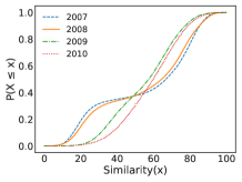
(a) Brazil

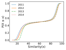
(b) United States

Figure 1: Cumulative Distribution Function of Edge Similarity.

In sum, we model the voting sessions in each country using two sets of networks, one network per year. Then, we use the Louvain Method [7] to identify ideological communities in each network. This method has been extensively used to detect network communities in various domains [15, 27, 9]. It is based on the optimization of modularity [26], a metric to evaluate the structure of clusters in a network. Modularity is large when the clustering is good and it can reach a maximum value of 1. In this study, we use modularity and party discipline as main metrics to assess the cohesiveness of the communities found. The former captures the quality of the result with respect to the topological structure of the communities in the network, whereas the latter, computed for the communities (rather than for individual parties), captures quality in terms of context semantics. In the next sections, we discuss the results of our analyses.

4 Identifying Ideological Communities

We start our discussion by tackling our first research question (RQ1) and characterizing the ideological communities discovered in both Brazilian and US networks. Table 2 shows an overview of all networks for both countries, presenting some topological properties [13], i.e., numbers of nodes (# of nodes) and edges (# of edges), number of connected components (# of CC), average shortest path length (SPL), average degree, clustering coefficient and density. Note the difference between the number of nodes in this table and the number of members in Table 1, corresponding to nodes that were removed after the edge filtering.

Table 2 also summarizes the characteristics of the ideological communities identified using the Louvain algorithm. In the four rightmost columns, it presents the number of communities identified, their modularity (Mod.) as well as average and standard deviation of the party discipline (Avg PD and SD PD), computed with respect to the ideological communities.

Starting with the Brazilian networks (top part of Table 2), we can observe great fluctuation in most topological metrics over the years, but, overall, the networks are sparse: the average shortest path length is short, the average clustering coefficient is moderate and the network density is low. Also, the number of communities identified is much smaller than the total number of parties (see Table 1) confirming the fragmentation and ideological overlap of multiple parties. Yet, the party discipline of these communities is, on average, very close to, and, in some cases, slightly larger than the values computed for the individual parties, despite a somewhat greater standard deviation observed across communities. Thus, these communities are indeed very cohesive in their voting patterns.

Table 2: Characterization of Networks and Ideological Communities

Brazil
Year	# of Nodes	# of Edges	# of CC	Avg. SPL	Avg. Degree	Avg. Clustering	Density	# of Comm.	Mod.	Avg. PD	SD PD
2003	342	9329	5	1.83	55.01	0.65	0.16	8	0.11	95.48%	2.22
2004	326	7079	2	1.90	43.43	0.62	0.13	4	0.14	92.68%	3.36
2005	359	7211	1	3.18	40.17	0.59	0.11	5	0.21	88.32%	3.64
2006	419	8613	1	2.47	41.11	0.61	0.09	4	0.36	90.50%	2.36
2007	427	11394	3	1.77	53.37	0.67	0.12	6	0.14	95.97%	1.26
2008	400	10180	2	1.62	50.90	0.70	0.12	5	0.08	95.78%	1.94
2009	434	10784	2	1.92	49.70	0.66	0.11	4	0.18	91.45%	3.49
2010	446	10151	1	2.42	45.52	0.64	0.10	4	0.19	92.01%	1.29
2011	408	11519	2	1.89	56.47	0.60	0.13	6	0.12	93.69%	3.76
2012	345	6527	3	2.47	46.11	0.48	0.11	4	0.33	87.00%	4.25
2013	449	10094	1	2.21	44.96	0.61	0.10	4	0.38	86.51%	4.18
2014	450	10036	1	2.18	44.60	0.58	0.09	3	0.43	91.14%	1.79
2015	490	12563	1	2.90	51.28	0.69	0.10	5	0.60	85.90%	3.11
2016	425	10159	2	1.44	47.81	0.66	0.11	4	0.38	92.62%	1.83
2017	396	9434	4	1.64	47.65	0.72	0.12	6	0.24	90.25%	3.16
United States
Year	# of Nodes	# of Edges	# of CC	Avg. SPL	Avg. Degree	Avg. Clustering	Density	# of Comm.	Mod.	Avg. PD	SD PD
2003	431	41892	2	1.11	194.39	0.95	0.45	2	0.48	93.60%	1.03
2004	426	40928	2	1.10	192.15	0.95	0.45	2	0.48	92.97%	0.55
2005	431	41892	2	1.10	194.39	0.95	0.45	2	0.48	92.60%	0.79
2006	426	41112	2	1.10	193.01	0.95	0.45	2	0.49	91.45%	0.33
2007	414	38471	2	1.12	185.85	0.94	0.45	2	0.44	91.55%	3.78
2008	424	40729	2	1.11	192.12	0.94	0.45	2	0.46	95.45%	1.97
2009	429	41698	2	1.15	194.40	0.94	0.45	2	0.40	93.86%	2.42
2010	420	39969	1	3.06	190.33	0.95	0.45	3	0.43	94.92%	1.86
2011	426	41119	2	1.18	193.05	0.96	0.45	3	0.44	90.31%	1.91
2012	417	40545	3	1.17	194.46	0.96	0.46	3	0.44	91.63%	1.86
2013	423	40921	2	1.11	193.48	0.96	0.45	2	0.47	93.23%	1.03
2014	418	40735	2	1.08	194.90	0.96	0.46	2	0.48	94.37%	0.34
2015	427	41890	2	1.09	196.21	0.95	0.46	2	0.47	94.40%	1.36
2016	423	40927	2	1.11	193.51	0.95	0.45	2	0.48	94.70%	1.36
2017	423	40928	2	1.09	193.51	0.95	0.45	2	0.46	96.02%	0.44

In contrast, the topological structure of the identified communities, as expressed by the modularity metric, is very weak, especially in the former years. That is, there is still a lot of similarity across members of different ideological communities. We note that in the former years the government had greater support from most parties, voting similarly in most sessions. Such approval dropped during a period of political turmoil that started in 2012, when the distinction of ideologies and opinions become more clear [33, 6]. This may explain why the modularity starts low and increases in the most recent years, when there is greater distinction between different communities. Note that this happens despite the large average party discipline maintained by the communities. That is, these two metrics provide complementary interpretations of the political scenario.

Turning our attention to the US (bottom part of Table 2), we note that, unlike in Brazil, most metrics remain roughly stable throughout the years. The networks are much more dense, with higher average clustering coefficient and density and shortest path length. The number of identified communities coincides with the number of connected components as well as with the number of political parties (see Table 1) in most years. These communities are more strongly structured, despite some ideological overlap, as expressed by moderate-to-large modularity value. Moreover, these communities are consistent in their ideologies, as expressed by large party disciplines, comparable to the original (party-level) ones. These metrics reflect the political behavior of a non-fragmented and stronger two-party system, quite unlike the Brazilian scenario.

In sum, in Brazil, the several parties can be grouped into just a few ideological communities, with strong disciplined members, although the separation between communities is not very clear. In the US, on the other hand, ideological communities are more clearly defined, both structurally and ideologically, though some inter-community similarity still remains.

5 Identifying Polarized Communities

As mentioned, the ideological communities identified in the previous section still share some similarity, particularly for the Brazilian case. In this section, we address our second research question (RQ2), with the aim of identifying polarized communities, i.e., communities that have a more clear distinction from the others in terms of voting behavior. To that end, we take a step further and consider that members of the same polarized community should not only be neighbors (i.e., similar to each other) but should also share most of their neighbors. Thus two members that, despite voting similar to each other, have mostly distinct sets of neighbors should not be in the same group.

To identify polarized communities, we start with the networks used to identify the ideological communities and compute the neighborhood overlap for each edge. The neighborhood overlap of an edge ($v_{i}$, $v_{j}$) is the ratio of the number of nodes that are neighbors of both $v_{i}$ and $v_{j}$ to the number of neighbors of at least one of $v_{i}$ or $v_{j}$ [13]. The neighborhood overlap of $v_{i}$ and $v_{j}$ is taken as an estimate of the strength of the tie between the two nodes. Edges with tie strength below (above) a given threshold are classified as weak (strong) ties. We consider that weak ties come from overlapping communities, and strong ties are edges within a polarized community. Thus, edges representing weak ties are removed. As before, all nodes that become isolated after this second filtering are also removed.

Once again the selection of the best neighborhood overlap threshold was not clear as it involves a complex tradeoff: larger thresholds lead to more closely connected communities and higher modularity, which is the goal, but also produce more sparse graphs, resulting in a larger number of isolated nodes which are disregarded. Thus, for each network, we selected a threshold that produced a good compromise between the two metrics. Figure 2 shows an example of this trade-off for one specific year (2017) in Brazil, with the selected threshold value shown in green. For Brazil, the selected threshold fell between 0.40 and 0.55, while for the United States this range was from 0.1 to 0.28. We then re-executed the Louvain algorithm to detect (polarized) communities in the new networks.

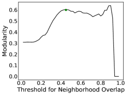
(a) Modularity

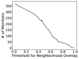
(b) Number of Members

Figure 2: Impact of Neighborhood Overlap Threshold for Brazil, 2017 (Selected threshold in green.).

Table 3 presents the topological properties of the networks as well as the structural and ideological properties of the identified polarized communities, for both Brazil and US. Focusing first on the Brazilian networks (top part of the table), we see that the number of nodes with strong ties decreases drastically (by up to 66%) as compared to the networks analyzed in Section 4. This indicates the large presence of House members that, despite great similarity with other members, are not strongly tied (as defined above) to them, and thus do not belong to any polarized community. The number of connected components dropped for some years and increased for others, suggesting that some components in the first set of networks were composed of structurally weaker communities or of multiple smaller communities. Network density, average shortest path length, and clustering coefficient also dropped, indicating more sparse networks, as expected.

Table 3: Characterization of Strongly Tied Networks and Polarized Communities

Brazil
Year	# of Nodes	# of Edges	# of CC	Avg. SPL	Avg. Degree	Avg. Clustering	Density	# of Comm.	Mod.	Avg. PD	SD PD
2003	186	1436	1	1.48	15.44	0.38	0.08	4	0.35	97.78%	0.86
2004	154	866	1	1.52	11.25	0.33	0.07	5	0.36	97.11%	0.57
2005	119	1210	2	1.19	20.34	0.59	0.17	4	0.37	95.40%	0.93
2006	136	590	10	1.37	8.68	0.52	0.06	12	0.57	96.62%	2.16
2007	175	977	3	1.68	11.17	0.32	0.06	6	0.44	97.31%	1.36
2008	216	1019	2	1.94	9.44	0.23	0.04	5	0.42	97.11%	0.46
2009	209	1217	1	1.30	11.65	0.41	0.05	5	0.56	94.57%	1.67
2010	225	726	6	1.45	6.45	0.22	0.02	11	0.51	94.31%	1.80
2011	250	1891	1	1.78	15.13	0.31	0.06	4	0.40	96.56%	0.86
2012	145	1151	3	1.84	29.82	0.48	0.11	6	0.37	94.42%	1.98
2013	318	4437	5	1.77	27.91	0.58	0.08	9	0.47	91.30%	2.17
2014	287	1672	3	1.37	11.65	0.41	0.04	5	0.63	94.04%	1.28
2015	372	6290	6	1.41	33.82	0.64	0.09	9	0.64	93.93%	1.70
2016	269	1726	3	1.43	12.83	0.44	0.04	8	0.63	95.08%	1.21
2017	227	1631	5	1.58	14.37	0.44	0.06	6	0.60	95.25%	2.01
United States
Year	# of Nodes	# of Edges	# of CC	Avg. SPL	Avg. Degree	Avg. Clustering	Density	# of Comm.	Mod.	Avg. PD	SD PD
2003	431	41872	2	1.11	194.30	0.95	0.45	2	0.47	93.60%	1.03
2004	426	40741	2	1.12	191.27	0.95	0.45	2	0.48	92.97%	0.55
2005	431	41886	2	1.11	194.37	0.95	0.45	2	0.47	92.60%	0.79
2006	426	41073	2	1.10	192.83	0.95	0.45	2	0.48	91.45%	0.33
2007	414	38462	2	1.12	185.81	0.94	0.44	2	0.42	91.55%	3.78
2008	423	40708	2	1.11	192.47	0.95	0.45	2	0.43	95.49%	1.93
2009	428	41690	2	1.15	194.81	0.94	0.45	2	0.40	93.89%	2.45
2010	418	39958	2	1.13	191.19	0.95	0.45	3	0.43	94.86%	1.97
2011	422	41112	2	1.15	194.84	0.97	0.46	3	0.45	90.01%	3.16
2012	413	40529	2	1.07	196.27	0.97	0.47	3	0.44	91.70%	2.17
2013	421	40910	2	1.10	194.35	0.96	0.46	2	0.46	93.32%	0.94
2014	417	40717	2	1.08	195.29	0.96	0.46	2	0.48	94.40%	0.38
2015	424	41759	2	1.08	196.98	0.95	0.46	2	0.47	94.53%	1.41
2016	418	40890	2	1.08	195.65	0.96	0.46	3	0.46	95.67%	0.80
2017	421	40923	2	1.08	194.41	0.95	0.46	2	0.48	95.37%	0.11

The number of polarized communities somewhat differs from the number of communities obtained when all (strong and weak) ties are considered, increasing in most years. This suggests that some ideological communities identified in Section 4 may be indeed formed by multiple more closely connected subgroups. Yet, those numbers are still smaller than the number of parties in each year (Table 1). Moreover, compared to the ideological communities first analyzed, the polarized communities are stronger both structurally and ideologically, as expressed by larger values of modularity and average party discipline.

For the US case, the numbers in Table 3 are very similar to those in Table 2. Less than 2% of the nodes have only weak ties and were removed from the networks in all years. Thus, almost all members have strong ties to each other, building ideological communities that are, in general, very polarized.

In sum, despite the fragmented party system, polarization can be observed in Brazil, to some degree, in a number of smaller strongly tied communities. In the US, on the other hand, almost all members and communities are very polarized.

6 Temporal Analysis

We finally turn to RQ3 and investigate how the polarized communities evolve over time. To that end, we compute two complementary metrics, namely persistence and normalized mutual information [32, 36], for each pair of consecutive years. We define the persistence from year $x$ to $x$+$1$ as the fraction of all members of polarized communities in $x$ who remained in some polarized community in $x$+$1$. A persistence equal to 100% implies that all members of polarized communities in $x$ remained in some polarized community in $x+1$. Yet, the membership of individual communities may have changed as members may have moved to different communities. To assess the extent of change in community membership over consecutive years, we compute the normalized mutual information (NMI) over the communities, taking only members who persisted over the two years.

NMI is based on Shannon entropy of information theory [31]. Given two sets of partitions $X$ and $Y$, defining community assignments for nodes, the mutual information of $X$ and $Y$ can be thought as the informational “overlap” between $X$ and $Y$, or how much we learn about $Y$ from $X$ (and about $X$ from $Y$). Let $P(x)$ be the probability that a node picked at random is assigned to community $x$, $P(x,y)$ be the probability that a node picked at random is assigned to both $x$ in $X$ and $y$ in $Y$. Also, let $H(X)$ be the Shannon entropy for $X$ defined as $H(X)=-\sum_{x}P(x)logP(x)$. The NMI of $X$ and $Y$ is defined as:

$$NMI(X,Y)=\frac{\sum_{x}\sum_{y}P(x,y)log\frac{P(x,y)}{P(x)P(y)}}{\sqrt{H(X)H(Y)}}$$ (2)

NMI ranges from 0 (all members changed their communities) to 1 (all members remained in the same communities).

Table 4 shows persistence (Pers) and NMI results for all pairs of consecutive years and both countries. For Brazil (BR), the values of persistence varied over the years, ranging from 46% to 80%. Thus, a significant number of new nodes join polarized communities every year. Indeed, in most years, roughly half of the members of polarized communities are newcomers. Moreover, the values of NMI are small, especially in the earlier years, reflecting great change also in terms of nodes switching communities. This is consistent with a period of less clear distinction between the communities and weaker polarization, as discussed in the previous sections. Since 2012, the values of NMI fall around 0.6, reflecting greater stability in community membership. For the US, on the other hand, both persistence and NMI are very large, approaching the maximum (1). Almost all members persist in their polarized communities over the years.

Table 4: Temporal Evolution of Polarized Ideological Communities.

Sequential Years		2003 2004	2004 2005	2005 2006	2007 2008	2008 2009	2009 2010	2011 2012	2012 2013	2013 2014	2015 2016	2016 2017
BR	Pers.	58.24%	46.30%	53.04%	68.26%	63.80%	61.38%	80.08%	67.87%	61.23%	57.85%	57.47%
	NMI	0.14	0.16	0.20	0.22	0.18	0.26	0.14	0.59	0.56	0.65	0.58
US	Pers.	98.13%	90.80%	98.36%	97.57%	86.74%	96.24%	96.18%	96.76%	97.85%	97.63%	86.26%
	NMI	0.97	0.97	1.00	1.00	1.00	0.94	0.96	0.80	1.00	0.97	0.98

A visualization of some of these results is shown in Figure 3 which presents the flow of nodes across polarized communities over the years of 2015 to 2017 in Brazil and in the US. Each vertical line represents a community, and its length represents the number of members belonging to that community who persisted in some polarized community in the following year. Thus, communities for which all members did not persist in any polarized community in the following year are not represented in the figure. Recall that, according to Table 3, the number of polarized communities in Brazil in 2015, 2016 and 2017 was 9, 8 and 6, respectively. A cross-analysis of these results with Figure 3a indicates that members of only 4 out of 9 polarized communities in 2015 persisted polarized in the following year. Moreover, two polarized communities in 2016 were composed of only newcomers and both communities disappeared in 2017 (as they do not appear in the figure). Similarly, one polarized community in 2017 was composed of only newcomers. The figure also shows a great amount of switching, merging and splitting across communities over the years. Figure 3b, on the other hand, illustrates the greater stability of community membership in the US.

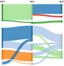
(a) Brazil

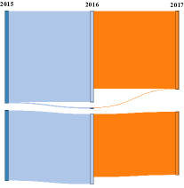
(b) United States

Figure 3: Dynamics of Polarized Communities over 2015-2017.

7 Conclusions and Future Work

We have proposed a methodology to analyze the formation and evolution of ideological and polarized communities in party systems, applying it to two strikingly different political contexts, namely Brazil and the US. Our analyses showed that the large number of political parties in Brazil can be reduced to only a few ideological communities, maintaining their original ideological properties, that is well disciplined communities, with a certain degree of redundancy. These communities have distinguished themselves both structurally and ideologically in the recent years, a reflection of the transformation that Brazilian politics has been experiencing since 2012. For the US, the country’s strong and non-fragmented party system leads to the identification of ideological communities in the two main parties throughout the analyzed period. However, there are still some highly similar links crossing the community boundaries. Moreover, for some years, a third community emerged, without however affecting the strong discipline, ideology and community structure of the American party system.

We then took a step further and focused on polarized communities by considering only tightly connected groups of nodes. We found that in Brazil, despite the party fragmentation and the existence of some degree of similarity even across the identified ideological communities, it is still possible to find a subset of members that organize themselves into strongly polarized ideological communities. However, these communities are highly dynamic, changing a large portion of their membership over consecutive years. In the US, on the other hand, most ideological communities identified are indeed highly polarized and their membership remain mostly unchanged over the years.

As future work, we intend to further analyze ideological communities in our datasets by characterizing members in terms of their centrality as well as proposing new metrics of tie strength for this particular domain. We also intend to extend our study to other party systems.

Acknowledgments

This work was partially supported by the FAPEMIG-PRONEX-MASWeb project – Models, Algorithms and Systems for the Web, process number APQ-01400-14, as well as by the National Institute of Science and Technology for the Web (INWEB), CNPq and FAPEMIG.

References

[1]
Agathangelou, P., Katakis, I., Rori, L., Gunopulos, D., Richards, B.:
Understanding online political networks: The case of the far-right and
far-left in greece. In: International Conference on Social Informatics. pp.
162–177. Springer (2017)
[2]
Ames, B.: The deadlock of democracy in Brazil. University of Michigan Press
(2009)
[3]
Andris, C., Lee, D., Hamilton, M.J., Martino, M., Gunning, C.E., Selden, J.A.:
The rise of partisanship and super-cooperators in the u.s. house of
representatives. PLOS ONE 10(4), 1–14 (04 2015)
[4]
Arinik, N., Figueiredo, R., Labatut, V.: Signed graph analysis for the
interpretation of voting behavior. International Workshop on Social Network
Analysis and Digital Humanities (2017)
[5]
Baldassarri, D., Gelman, A.: Partisans without constraint: Political
polarization and trends in american public opinion. American Journal of
Sociology 114(2), 408–446 (2008)
[6]
BBC: Brazil profile - timeline (2018),
http://www.bbc.com/news/world-latin-america-19359111
[7]
Blondel, V.D., Guillaume, J.L., Lambiotte, R., Lefebvre, E.: Fast unfolding of
communities in large networks. Journal of statistical mechanics: theory and
experiment 2008(10) (2008)
[8]
Budge, I., Laver, M.J.: Party policy and government coalitions. Springer (2016)
[9]
Cai, Q., Ma, L., Gong, M., Tian, D.: A survey on network community detection
based on evolutionary computation. Int. J. Bio-Inspired Comput. 8(2),
84–98 (May 2016)
[10]
Cherepnalkoski, D., Karpf, A., Mozetič, I., Grčar, M.: Cohesion and coalition
formation in the european parliament: Roll-call votes and twitter activities.
PLOS ONE 11(11), 1–27 (11 2016)
[11]
Dal Maso, C., Pompa, G., Puliga, M., Riotta, G., Chessa, A.: Voting behavior,
coalitions and government strength through a complex network analysis. PLOS
ONE 9, 1–13 (12 2015)
[12]
Darwish, K., Magdy, W., Zanouda, T.: Trump vs. hillary: What went viral during
the 2016 us presidential election. In: International Conference on Social
Informatics. pp. 143–161. Springer (2017)
[13]
Easley, D., Kleinberg, J.: Networks, crowds, and markets: Reasoning about a
highly connected world. Cambridge University Press (2010)
[14]
Fiorina, M.P., Abrams, S.J.: Political polarization in the american public.
Annual Review of Political Science 11(1), 563–588 (2008)
[15]
Fortunato, S.: Community detection in graphs. Physics Reports 486(3), 75 –
174 (2010)
[16]
Granovetter, M.S.: The strength of weak ties. In: Social networks, pp.
347–367. Elsevier (1977)
[17]
Hix, S., Noury, A., Roland, G.: Power to the parties: cohesion and competition
in the european parliament, 1979–2001. British Journal of Political Science
35(2), 209–234 (2005)
[18]
Jones, J.J., Settle, J.E., Bond, R.M., Fariss, C.J., Marlow, C., Fowler, J.H.:
Inferring tie strength from online directed behavior. PLOS ONE 8(1), 1–6
(01 2013)
[19]
Levorato, M., Frota, Y.: Brazilian Congress structural balance analysis.
Journal of Interdisciplinary Methodologies and Issues in Science Graphs
and social systems (Mar 2017)
[20]
Mainwaring, S., Shugart, M.S.: Presidentialism and democracy in Latin America.
Cambridge University Press (1997)
[21]
Mann, T.E., Ornstein, N.J.: It’s even worse than it looks: How the American
constitutional system collided with the new politics of extremism. Basic
Books (2016)
[22]
McGee, J., Caverlee, J., Cheng, Z.: Location prediction in social media based
on tie strength. In: Proceedings of the 22Nd ACM International Conference on
Information & Knowledge Management. pp. 459–468. CIKM ’13, ACM, New York,
NY, USA (2013)
[23]
Vaz de Melo, P.O.S.: How many political parties should brazil have? a
data-driven method to assess and reduce fragmentation in multi-party
political systems. PLOS ONE 10(10), 1–24 (10 2015)
[24]
Mendonça, I., Trouve, A., Fukuda, A.: Exploring the importance of negative
links through the european parliament social graph. In: Proceedings of the
2017 International Conference on E-Society, E-Education and E-Technology. pp.
1–7. ICSET 2017, ACM, New York, NY, USA (2017)
[25]
Moody, J., Mucha, P.J.: Portrait of political party polarization. Network
Science 1(1), 119–121 (2013)
[26]
Newman, M.E.J.: Modularity and community structure in networks. Proceedings of
the National Academy of Sciences 103(23), 8577–8582 (2006)
[27]
Plantié, M., Crampes, M.: Survey on social community detection. In: Social
media retrieval, pp. 65–85. Springer (2013)
[28]
Porter, M.A., Mucha, P.J., Newman, M.E.J., Warmbrand, C.M.: A network analysis
of committees in the u.s. house of representatives. Proceedings of the
National Academy of Sciences 102(20), 7057–7062 (2005)
[29]
Rossetti, G., Cazabet, R.: Community discovery in dynamic networks: A survey.
ACM Comput. Surv. 51(2), 35:1–35:37 (Feb 2018)
[30]
Sartori, G.: Parties and party systems: A framework for analysis. ECPR press
(2005)
[31]
Shannon, C.E.: A mathematical theory of communication. ACM SIGMOBILE Mobile
Computing and Communications Review 5(1), 3–55 (2001)
[32]
Vinh, N.X., Epps, J., Bailey, J.: Information theoretic measures for
clusterings comparison: Variants, properties, normalization and correction
for chance. Journal of Machine Learning Research 11(Oct), 2837–2854 (2010)
[33]
Vox: Brazil’s political crisis, explained (2016),
https://www.vox.com/2016/4/21/11451210/dilma-rousseff-impeachment
[34]
Wang, Y., Feng, Y., Hong, Z., Berger, R., Luo, J.: How polarized have we
become? a multimodal classification of trump followers and clinton followers.
In: International Conference on Social Informatics. pp. 440–456. Springer
(2017)
[35]
Waugh, A.S., Pei, L., Fowler, J.H., Mucha, P.J., Porter, M.A.: Party
polarization in congress: A social networks approach. arXiv preprint
arXiv:0907.3509 (2009)
[36]
Wei, W., Carley, K.M.: Measuring temporal patterns in dynamic social networks.
ACM Trans. Knowl. Discov. Data 10(1), 9:1–9:27 (Jul 2015)
[37]
Wiese, J., Min, J.K., Hong, J.I., Zimmerman, J.: ”you never call, you never
write”: Call and sms logs do not always indicate tie strength. In:
Proceedings of the 18th ACM Conference on Computer Supported Cooperative Work
and Social Computing. pp. 765–774. CSCW ’15, ACM, New York, NY, USA (2015)