The Impact of Photometric Redshift Errors on Lensing Statistics in Ray-Tracing Simulations

Abstract

Weak lensing surveys are reaching sensitivities at which uncertainties in the galaxy redshift distributions $n(z)$ from photo-$z$ errors degrade cosmological constraints. We use ray-tracing simulations and a simple treatment of photo-$z$ errors to assess cosmological parameter biases from uncertainties in $n(z)$ in an LSST-like survey. We use the power spectrum and the abundance of lensing peaks to infer cosmological parameters, and find that the former is somewhat more resilient to photo-$z$ errors. We place conservative lower limits on the survey size at which different types of photo-$z$ errors degrade $\Lambda$CDM ($w$CDM) parameter constraints by $50\%$. A residual constant photo-$z$ bias of $|\delta z|<0.003(1+z)$, satisfying the current LSST requirement, does not significantly degrade constraints for surveys smaller than $\approx$$1300$ ($\approx$$490$) deg² using lensing peaks and $\approx$$6500$ ($\approx$$4900$) deg² using the power spectrum. Adopting a recent prediction for LSST’s full photo-$z$ probability distribution function (PDF), we find that simply approximating $n(z)$ with the photo-$z$ galaxy distribution directly computed from this PDF would degrade surveys as small as $\approx$$60$ ($\approx$$65$) deg² using lensing peaks or the power spectrum. Assuming that the centroid bias in each tomographic redshift bin can be removed from the photo-$z$ galaxy distribution, using lensing peaks or the power spectrum still degrades surveys larger than $\approx$200 ($\approx$255) or $\approx$248 ($\approx$315) deg². These results imply that the expected broad photo-$z$ PDF significantly biases parameters, which needs to be further mitigated using more sophisticated photo-$z$ treatments.

1 Introduction

Upcoming weak lensing (WL) surveys hold great promise for probing the nature of dark energy and constraining cosmological parameters to unprecedented precision. They draw their constraining power from measuring cosmic shear – small distortions in the shapes of distant galaxies caused by gravitational lensing by foreground structures – which is sensitive to the histories of both the expansion rate and the growth of structure.

Current WL surveys are reaching sizes where the constraints on $\Omega_{m}$ and $\sigma_{8}$ are becoming competitive with other cosmology probes. Measurements of the shear 2-point correlation function (2PCF) for the recently completed Canada-France-Hawaii-Telescope Legacy Survey (CFHTLenS) used 4.2 million galaxies distributed over 154 ${\rm deg}^{2}$ (Kilbinger et al., 2013). Constraints have also been measured in ongoing surveys such as the Kilo Degree Survey (KiDS) (de Jong et al., 2013), the Dark Energy Survey (DES) (DES Collaboration, 2005), and Subaru Hyper Suprime-Cam (HSC) (Aihara et al., 2018). Current measurements of two-point statistics in each survey have used 15 million galaxies distributed over 450 ${\rm deg}^{2}$ (Hildebrandt et al., 2017), 26 million galaxies distributed across 1321 ${\rm deg}^{2}$ (Troxel et al., 2017), and 9 million galaxies distributed over 137 ${\rm deg}^{2}$ (Hikage et al., 2018). Upon completion these surveys will span 1500 ${\rm deg}^{2}$, 5000 ${\rm deg}^{2}$, and 1400 ${\rm deg}^{2}$, respectively.

Moreover, when combined with other cosmological probes, such as the cosmic microwave background or galaxy clustering, current WL surveys are beginning to provide useful constraints on $w$ (e.g. DES Collaboration et al., 2017). Data from current surveys has also been used compute non-Gaussian summary statistics, such as lensing peaks (e.g Liu et al., 2015a, b; Kacprzak et al., 2016; Martinet et al., 2018), higher-order mixed moments (e.g. Petri et al., 2015), higher-order correlation functions (e.g. Fu et al., 2014), and Minkowski functionals (e.g Petri et al., 2015). These summary statistics provide the opportunity to increase the amount of cosmological information extracted from cosmic shear. More recently, studies have explored possible additional features residing in simulated lensing maps, using convolutional neural networks (e.g. Schmelzle et al., 2017; Gupta et al., 2018; Ribli et al., 2018).

Upcoming WL surveys such as the full DES, Euclid (Laureijs et al., 2011), LSST (Ivezić et al., 2008; LSST Science Collaboration et al., 2009), and WFIRST (Spergel et al., 2015), are expected to measure cosmic shear using $\sim 10^{8}-10^{9}$ galaxies. Cosmological constraints from these surveys are likely to be limited by systematic errors (Albrecht et al., 2006). One example is the systematic error arising from uncertainties and biases in the photometric redshift (photo-$z$) measurements.

Due to the prohibitive cost of acquiring spectroscopic redshifts for every galaxy, weak lensing surveys rely on photo-$z$’s to estimate the underlying true galaxy redshift distribution $n_{\rm true}(z)$. Because photo-$z$’s are estimated with a finite set of photometric filters, their errors vary as functions of $z$, brightness, and morphological type. Typically these errors are divided into bias (the offset between the median/mean photo-$z$ and the true $z$), the scatter of photo-$z$ measurements about the median photo-$z$ at a given $z$, and the catastrophic photo-$z$ errors (outlier photo-$z$’s that can arise from multimodal photo-$z$ distributions). On the observational side, WL surveys perform complex analyses to reduce errors in estimates of $n_{\rm true}(z)$. However, theoretical work is required to understand how small errors in these estimates propagate into cosmology parameter errors.

Extensive work has been done to study the impact of photo-$z$ errors on constraints from WL surveys and techniques to mitigate it (e.g. Ma et al., 2006; Huterer et al., 2006; Bridle & King, 2007; Jain et al., 2007; Abdalla et al., 2008; Ma & Bernstein, 2008; Kitching et al., 2008; Bernstein & Huterer, 2010; Hearin et al., 2010; Hearin et al., 2012; Cunha et al., 2012, 2014; de Putter et al., 2014; Shirasaki & Yoshida, 2014; Petri et al., 2016; Rau et al., 2017). The vast majority of works used a Fisher analysis to study the impact of photo-$z$ errors on either the lensing 2PCF or the power spectrum, and on the cosmological parameters inferred from these observables. Notable exceptions include Huterer et al. (2006) who studied the impact on the convergence bispectrum, Kitching et al. (2008) who exclusively studied the impact on constraints obtained with the shear-ratio method and 3D cosmic shear, Shirasaki & Yoshida (2014) who employed ray-tracing simulations to assess the impact on Minkowski Functionals and Petri et al. (2016) who used ray-tracing simulations to study the impact on both peak counts and higher-order mixed moments of the convergence field. Because they have different dependence on the underlying galaxy distributions, non-Gaussian summary statistics are impacted in different ways by photo-$z$ errors and offer the possibility of self-calibration (Huterer et al., 2006; Petri et al., 2016).

Ray-tracing simulations have also been used to assess the effects of other kinds of systematics on cosmological constraints of non-Gaussian Statistics (e.g. Shirasaki et al., 2013; Liu et al., 2014; Petri et al., 2014).

In this paper, we use ray-tracing simulations, without assuming a linear dependence of summary statistics on cosmology, to study the impact of both a constant uncalibrated photo-$z$ bias and of a more realistic full photo-$z$ probability distribution function (PDF; adapted from Rhodes et al. 2017, based on a simulated spectroscopic calibration sample for LSST). Our approach is to use our simulations to produce a mock lensing dataset; we then produce an independent set of simulations, over a large grid of cosmologies, which all have the “wrong” redshifts, and which we use to fit the mock data. We quantify the resulting degradation in the cosmological parameter constrains inferred from the tomographic convergence peak counts in an LSST-like survey. We also present a side-by-side analysis of the tomographic convergence power spectrum, to compare the susceptibility of these two observables to photo-$z$ errors.

We organise this paper as follows: In § 2 we describe our simulations, the construction of the convergence maps, the calculation of the summary statistics, our model of the photo-$z$ errors, and scaling up our forecast degradations to large LSST-like surveys. We then describe and discuss our results in § 3 and § 4, respectively. Finally, in § 5 we summarise our main conclusions and the implications of this work.

Our analysis is the first step towards a full assessment, based on simulations, to identify photo-$z$ requirements for peak counts, and to design the best strategy to mitigate the impact of photo-$z$ errors.

Table 1: This table summarises details of the Single-$z$ dataset and Tomographic dataset. We define $\hat{\kappa}_{\rm obs}({\boldsymbol{\theta}}_{p})$, $\hat{\kappa}_{r}^{\rm fid}({\boldsymbol{\theta}}_{p})$ and $\hat{\kappa}_{r}({\boldsymbol{\theta}}_{p};{\bf p})$ as the as the convergence maps used as mock observations, to construct the covariance matrix, and as theoretical predictions for inference, respectively. The first two are evaluated in the fiducial cosmology, while the last are evaluated for different combinations of cosmological parameters ${\bf p}$. Corresponding shear catalogues are denoted by $\hat{{\boldsymbol{\gamma}}}_{\rm obs}({\boldsymbol{\theta}}_{g},z_{g})$, $\hat{{\boldsymbol{\gamma}}}_{r}^{fid}({\boldsymbol{\theta}}_{g},z_{g})$ and $\hat{{\boldsymbol{\gamma}}}_{r}({\boldsymbol{\theta}}_{g},z_{g};{\bf p})$. Note that ${\boldsymbol{\theta}}_{p}$ indicates the location of a pixel on a two-dimensional convergence map, while ${\boldsymbol{\theta}}_{g}$ and $z_{g}$ indicate the apparent angular position and redshift of a galaxy in a shape catalogue.

	Single-$z$ dataset	Tomographic dataset
Gadget-2 comoving volume	$(240\ h^{-1}{\rm Mpc})^{3}$	$(260\ h^{-1}{\rm Mpc})^{3}$
Comoving lens plane spacing	$80\ h^{-1}{\rm Mpc}$	$120\ {\rm Mpc}$
Simulationsa: $\hat{\kappa}_{\rm obs}({\boldsymbol{\theta}}_{p})$ & $\hat{{\boldsymbol{\gamma}}}_{\rm obs}({\boldsymbol{\theta}}_{g},z_{g})$	Z17	Simulations were run for this work
Simulationsa: $\hat{\kappa}_{r}^{\rm fid}({\boldsymbol{\theta}}_{p})$ & $\hat{{\boldsymbol{\gamma}}}_{r}^{fid}({\boldsymbol{\theta}}_{g},z_{g})$	Same simulation used for $\hat{\kappa}_{\rm obs}({\boldsymbol{\theta}}_{p})$	P16
Simulationsa: $\hat{\kappa}_{r}({\boldsymbol{\theta}}_{p};{\bf p})$ & $\hat{{\boldsymbol{\gamma}}}_{r}({\boldsymbol{\theta}}_{g},z_{g};{\bf p})$	161 of the sampled cosmologies from Z16 & simulation for $\hat{\kappa}_{\rm obs}({\boldsymbol{\theta}}_{p})$	All 100 cosmologies from P16 [does not include simulation for $\hat{{\boldsymbol{\gamma}}}_{r}^{fid}({\boldsymbol{\theta}}_{g},z_{g})$]
photo-$z$ galaxy distribution	$n_{\rm ph}(z)=25\,{\rm arcmin}^{-2}\delta(z-1)$	Equation 1
Number of realisations ($N_{r}$)	500	16000 [for $\hat{{\boldsymbol{\gamma}}}_{r}({\boldsymbol{\theta}}_{g},z_{g};{\bf p})$ & $\hat{{\boldsymbol{\gamma}}}_{r}^{fid}({\boldsymbol{\theta}}_{g},z_{g})$] and 1000 [for $\hat{{\boldsymbol{\gamma}}}_{\rm obs}({\boldsymbol{\theta}}_{g},z_{g})$]
Tomography	No	Yes - see Fig. 1 and Table 2
$\kappa$ map Gaussian smoothing scale	$\sqrt{0.5}$ arcmin	1 arcmin
$\kappa$ map resolution	$1024^{2}$	$492^{2}$
$\kappa$ map Field of View	$(3.5{\rm deg})^{2}$	$(3.36{\rm deg})^{2}$
Summary statistics	$n_{\rm pk}$	$n_{\rm pk}$ and $P^{\kappa\kappa}$
PCA	No	Only for $P^{\kappa\kappa}$
Role of interpolator	Interpolate the $\chi^{2}$ between the observation and each sampled cosmology	Interpolate the summary statistics between each sampled cosmology
Inferred Cosmological Models	$\Lambda$CDM	$\Lambda$CDM and $w$CDM
Uniform Prior Range	$\Omega_{m}\in[0.16,0.6]$, $\sigma_{8}\in[0.15,1.25]$	$\Omega_{m}\in[0.2,0.5]$, $w\in[-1.5,-0.5]$ (for $w$CDM inference), $\sigma_{8}\in[0.5,1.2]$
Sampling of Inference Grid	$\Delta p=0.001$ in each parameter (Z16)	See Table 3

^a Indicate the works from which the simulations used to construct different convergence and shear maps are adopted.

2 Methodology

In our analysis, we use ray-tracing simulations coupled with N-body DM-only simulations to construct pixelized convergence ($\kappa$) maps. The convergence is proportional to the distance-weighted over-density along the light’s path. The $\kappa$ maps are then used to compute weak lensing summary statistics ${\bf d}$. Our basic approach is to produce these statistics in a fiducial cosmology ${\bf p}_{0}$, representing a mock observation. ${\bf p}_{0}$ is a $\Lambda$CDM cosmology consistent with WMAP results (Hinshaw et al., 2013), with the parameter values $(h,\Omega_{m},\Omega_{\Lambda},\Omega_{b},w,\sigma_{8},n_{s})=(0.72,$ $0.26,$ $0.74,$ $0.0046,$ $-1,$ $0.8,$ $0.96)$. We then separately produce a different set of the maps and statistics, over a large grid of spatially flat cosmological models, $\{{\bf p_{i}}\}$; these represent the theoretical predictions used to fit the mock observation and to infer cosmological parameters ${\bf p}\equiv(\Omega_{m},w,\sigma_{8})$. The mock observation and the theoretical predictions have different redshift-distributions, which results in biases in the best-fit parameters.

Our analysis involves the construction of $N_{r}$ realisations of three types of pixelized convergence maps: $\hat{\kappa}_{\rm obs}({\boldsymbol{\theta}}_{p},\bar{z}_{b})$, $\hat{\kappa}_{r}^{\rm fid}({\boldsymbol{\theta}}_{p},\bar{z}_{b})$ and $\hat{\kappa}_{r}({\boldsymbol{\theta}}_{p},\bar{z}_{b};{\bf p})$. To be consistent with the notation of Petri et al. (2016), $\hat{\kappa}$ denotes convergence maps with shape noise added while ${\boldsymbol{\theta}}_{p}$ and $\bar{z}_{b}$ indicate the coordinates of a pixel and the tomographic redshift bin, respectively. $\hat{\kappa}_{\rm obs}({\boldsymbol{\theta}}_{p},\bar{z}_{b})$ refers to the maps constructed from ${\bf p}_{0}$ which we use to produce summary statistics for our the mock observation. $\hat{\kappa}_{r}^{\rm fid}({\boldsymbol{\theta}}_{p},\bar{z}_{b})$ is also constructed for ${\bf p}_{0}$, however we use the calculated ${\bf d}$ to compute a covariance matrix over its $N_{r}$ realisations. This is necessary to evaluate parameter likelihoods. Finally, we construct $\hat{\kappa}_{r}({\boldsymbol{\theta}}_{p},\bar{z}_{b};{\bf p})$ for each cosmology in $\{{\bf p_{i}}\}$ and use it compute the expectation value of the summary statistics ${\bf d}({\bf p})$ (again over $N_{r}$ realisations). We use them as a theoretical prediction tool that interpolates either the ${\bf d}$ themselves or the goodness of fit of a mock observation as a function of cosmology.

To assess the impact of photo-$z$ errors, we use a single galaxy distribution $n(z)$ to produce the covariance matrix and interpolator, and examine the biases in the constraints for mock observations computed with different galaxy distributions. These distributions represent different types of photo-$z$ errors, including a residual photo-$z$ bias, and a more realistic full photo-$z$ PDF simulated for LSST. We quantify the degradation in the cosmological parameter constrains inferred from the tomographic $\kappa$ peak counts in an LSST-like survey. We also present a side-by-side analysis of the tomographic $\kappa$ power spectrum, to compare the susceptibility of these two observables to photo-$z$ errors.

In § 2.1 and § 2.2, we review the steps to simulate cosmic shear for an arbitrary galaxy distribution in an arbitrary cosmology ${\bf p}$, and to prepare convergence ($\kappa$) maps suitable for computing summary statistics. We describe the steps to calculate summary statistics in § 2.3. In § 2.4, we describe how we model photo-$z$ errors, and finally, in § 2.5 we describe cosmological parameter inference.

Our analysis makes use of two separate datasets, summarised in Table 1, mostly consisting of simulation data we adopt from prior studies. Each dataset has an independent $\{{\bf p_{i}}\}$. Our first dataset includes data from Zorrilla Matilla et al. (2016, hereafter Z16) and Zorrilla Matilla et al. (2017, Z17). Z16 studied the accuracy of using lensing peak predictions made with camelus (Lin & Kilbinger, 2015) to infer cosmology, while Z17 studied the individual and combined dependence of weak lensing on the growth of structure and on the universe’s expansion history. Both of these studies used source galaxies at a single redshift ($z=1$), and did not include redshift tomography. We will hereafter refer to the combined dataset as the “Single-$z$” dataset. We also remove the redshift-bin dependence from the notation in this dataset, and denote $\hat{\kappa}_{r}({\boldsymbol{\theta}}_{p},\bar{z}_{b};{\bf p})$, $\hat{\kappa}_{r}^{\rm fid}({\boldsymbol{\theta}}_{p},\bar{z}_{b})$, and $\hat{\kappa}_{\rm obs}({\boldsymbol{\theta}}_{p},\bar{z}_{b})$ as $\hat{\kappa}_{r}({\boldsymbol{\theta}}_{p};{\bf p})$, $\hat{\kappa}_{r}^{\rm fid}({\boldsymbol{\theta}}_{p})$, and $\hat{\kappa}_{\rm obs}({\boldsymbol{\theta}}_{p})$.

For the Single-$z$ dataset, we directly take the ${\bf d}$ computed for 161 of our 162 cosmologies in $\{{\bf p_{i}}\}$ for $\hat{\kappa}_{r}({\boldsymbol{\theta}}_{p},\bar{z}_{b};{\bf p})$ from Z16. The remaining cosmology in $\{{\bf p_{i}}\}$ is ${\bf p}_{0}$. We reuse the single set of lens planes for ${\bf p}_{0}$ from Z17 to construct $\hat{\kappa}_{r}({\boldsymbol{\theta}}_{p};{\bf p}_{0})$, $\hat{\kappa}_{r}^{\rm fid}({\boldsymbol{\theta}}_{p})$, and $\hat{\kappa}_{\rm obs}({\boldsymbol{\theta}}_{p})$. This is because the lens planes in the fiducial model of Z16 were no longer available, and we need access to these lens planes in order to perform new ray-tracing calculations in the same model to slightly different redshifts, in the presence of photo-$z$ errors (see below).

The second, hereafter the “Tomography”, dataset almost entirely consists of data from Petri et al. (2016, P16). P16 forecasted cosmology constraints for a survey with an LSST-like galaxy distribution using the tomographic convergence power spectrum, tomographic peak counts and nine mixed moments for each of the tomographic convergence maps. Additionally, they made use of Principal Component analysis and briefly assessed the impact of uncorrected photo-$z$ errors on cosmological constraints. Our use of redshift tomography in this case necessitates the intermediate step of producing shape catalogues $\hat{{\boldsymbol{\gamma}}}_{r}({\boldsymbol{\theta}}_{g},z_{g};{\bf p})$, $\hat{{\boldsymbol{\gamma}}}_{r}^{fid}({\boldsymbol{\theta}}_{g},z_{g})$, and $\hat{{\boldsymbol{\gamma}}}_{\rm obs}({\boldsymbol{\theta}}_{g},z_{g})$ from which we ultimately construct $\hat{\kappa}_{r}({\boldsymbol{\theta}}_{p},\bar{z}_{b};{\bf p})$, $\hat{\kappa}_{r}^{\rm fid}({\boldsymbol{\theta}}_{p},\bar{z}_{b})$, and $\hat{\kappa}_{\rm obs}({\boldsymbol{\theta}}_{p},\bar{z}_{b})$. We call a noiseless catalogue a “Shear Catalogue” but adopt the convention of “Shape Catalog” in the presence of shape noise. For this dataset, we reuse the shear catalogues from P16 to generate $\hat{\kappa}_{r}({\boldsymbol{\theta}}_{p},\bar{z}_{b};{\bf p})$ and $\hat{\kappa}_{r}^{\rm fid}({\boldsymbol{\theta}}_{p},\bar{z}_{b})$. To generate $\hat{\kappa}_{\rm obs}({\boldsymbol{\theta}}_{p},\bar{z}_{b})$, we use new simulation data specifically generated for this work.

For completeness and convenience, we summarise the numerous small differences between the datasets in Table 1.

Figure 1: Illustrates the photo-$z$ distribution and the tomographic bins. The 10 bins are chosen to cover the range $0\leq z_{\rm ph}\leq 3$, and to each contain $10^{5}$ galaxies per simulated (3.5 deg)² field.

2.1 Cosmic shear simulations

In this subsection, we review how to simulate cosmic shear.

For a specific cosmology, ${\bf p}$, we start by running a Gadget-2 (Springel, 2005) dark matter-only N-body simulation. For the Single-$z$ (Tomographic) Dataset we use a box of comoving side length $L_{b}=240\ (260)\ h^{-1}{\rm Mpc}$ that contains $512^{3}$ DM particles with mass resolution of $\approx 10^{10}{\rm M}_{\sun}$ per particle. We slice each snapshot and apply random shifts and rotations to construct two-dimensional lens planes with comoving thickness $80\ h^{-1}{\rm Mpc}$ ($120$ Mpc). Next, we line up the planes perpendicular to the observer’s line of sight and calculate the induced $\kappa$ or shear ${\boldsymbol{\gamma}}$ for a source at redshift $z_{s}$, arising from deflections to the light rays by the sequence of lenses. We employ a multi-plane ray-tracing algorithm (Jain et al., 2000; Hilbert et al., 2009) to trace the path of light rays between the angular position at $z_{s}$ and its apparent angular position on the sky ${\boldsymbol{\theta}}$ at $z=0$. In practice, we use the LensTools package (Petri, 2016) to carry out all of these calculations for collections of sources distributed in angular position ${\boldsymbol{\theta}}$ and redshift $z_{s}$.

Throughout our analysis, we hold the distribution of the apparent galaxy sky positions constant and redo ray-tracing with varied galaxy redshift distributions. For the Single-$z$ (Tomographic) dataset, we assume that the galaxies are uniformly distributed across a $(3.5{\rm deg})^{2}$ region with an average number density $n_{g}$=25 ${\rm arcmin}^{-2}$ (22 ${\rm arcmin}^{-2}$). Due to computational limitations, we use a constant photo-$z$ galaxy distribution $n_{\rm ph}(z)$ for each simulation dataset and use it to act as the distribution of source redshifts for the majority of our ray-tracing simulations. This choice allows for the reuse of the summary statistic measurements from Z16 and the shear catalogues from P16. We defer further discussion of the interpretation of the fixed $n_{\rm ph}(z)$ to § 2.4.

In the Single-$z$ dataset, we assume a galaxy surface density redshift distribution, $d^{2}N_{tot}/(d\Omega dz_{\rm ph})$, referred to as $n_{\rm ph}(z)$ for simplicity, given by $n_{\rm ph}(z)=25{\rm arcmin}^{-2}\delta(z-1)$. In contrast, the analysis of the Tomographic dataset assumes a discrete distribution of $N_{tot}=10^{6}$ galaxies with photo-$z$’s restricted to $z_{\rm ph}$$\leq 3$ and otherwise drawn from

$$n_{\rm ph}(z)=n_{0}\left(\frac{z}{z_{0}}\right)^{2}{\rm exp}\left(-\frac{z}{z_{0}}\right).$$ (1)

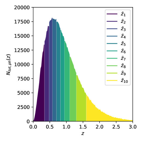
In this equation, $z_{0}=0.3$ was chosen to match the expected spectroscopic distribution for LSST and $n_{0}$ is chosen such that $N_{tot,ph}(z)=(3.5{\rm deg})^{2}\times n_{\rm ph}(z)$ integrates to $N_{tot}$. Figure 1 illustrates $N_{tot,ph}(z)$ for the Tomographic dataset and the 10 tomographic bins we employ in our analysis; each bin contains $10^{5}$ galaxies. Each of these distributions are identical to the spectroscopic redshift distributions $n_{\rm true}(z)$ used for ray-tracing in Z16 and P16.

Because the Single-$z$ dataset employs a simple distribution of galaxies, we are able to directly produce a $\kappa$ map covering a $(3.5{\rm deg})^{2}$ field with a resolution of $1024^{2}$ pixels from ray-tracing. To model the impact of shape noise, we follow van Waerbeke (2000) and Z16, and add a 2D array of values drawn from a zero-mean Gaussian distribution with standard deviation

$$\sigma=\sqrt{\frac{\sigma_{\epsilon}^{2}}{2n_{g}A_{pix}}}.$$ (2)

In this equation, $\sigma_{\epsilon}=0.4$ corresponds to the r.m.s intrinsic ellipticity, $n_{g}=25\,{\rm arcmin}^{-2}$ is the galaxy surface density and $A_{pix}=(0.042\,{\rm arcmin})^{2}$ is the solid angle enclosed by a pixel in the convergence map.

Ray-tracing for the Tomographic dataset produces a shear catalogue $\{{\boldsymbol{\gamma}}_{g}\}$ which includes the induced shear on each galaxy. We model the impact of shape noise as in P16. In a real survey we measure galaxy ellipticity ${\boldsymbol{\gamma}}_{m}={\boldsymbol{\gamma}}+{\boldsymbol{\epsilon}}_{\rm intrinsic}$, where ${\boldsymbol{\gamma}}$ is the true cosmic shear and ${\boldsymbol{\epsilon}}_{\rm intrinsic}$ is the intrinsic ellipticity of the galaxy (Schneider, 2005). Consequently, we transform our shear catalogue into a shape catalogue, which lists the measured ellipticity of each galaxy, by modelling ${\boldsymbol{\epsilon}}_{\rm intrinsic}$ with randomly drawn values from a zero-mean Gaussian with standard deviation $\sigma(z)=0.15+0.035z_{s}$ (Song & Knox, 2004).

By randomising the slices, shifts, and rotations used to create the lens planes and changing the random seed used for modelling shape noise, we can generate pseudo-random realisations of convergence maps and shape catalogues.

For the Single-$z$ dataset, we reuse lensing peaks for all cosmologies in $\{{\bf p_{i}}\}$ other than ${\bf p}_{0}$ from Z16. These lensing peaks were computed from $\hat{\kappa}_{r}({\boldsymbol{\theta}}_{p};{\bf p})$ which had been constructed using the above procedure. Because we want our mock observations, in the absence of photo-$z$ errors, to have $\chi^{2}=0$ when compared to the model-predicted lensing peaks, the lensing peaks computed from $\hat{\kappa}_{r}({\boldsymbol{\theta}}_{p};{\bf p}_{0})$, we need to use the same initial conditions and random seed to produce realisation $r$ of $\hat{\kappa}_{r}({\boldsymbol{\theta}}_{p};{\bf p}_{0})$ and $\hat{\kappa}_{\rm obs}({\boldsymbol{\theta}}_{p})$. Additionally, to produce the $\hat{\kappa}_{\rm obs}({\boldsymbol{\theta}}_{p})$ for different sets of photo-$z$ errors, we need access to the lens planes and random seed information. Since neither are available from Z16, we use the lens planes for ${\bf p}_{0}$ from Z17 and a different seed from Z16 to produce realisation $r$ $\hat{\kappa}_{r}({\boldsymbol{\theta}}_{p};{\bf p}_{0})$, $\hat{\kappa}_{r}^{\rm fid}({\boldsymbol{\theta}}_{p})$, and $\hat{\kappa}_{\rm obs}({\boldsymbol{\theta}}_{p})$. Our analysis of this dataset uses the summary statistics computed from $N_{r}=500$ realisations of each type of convergence map.

Our analysis using the Tomographic Dataset employs the suite of $N_{r}=16000$ realisations of $\hat{{\boldsymbol{\gamma}}}_{r}({\boldsymbol{\theta}}_{g},z_{g};{\bf p})$ and $\hat{{\boldsymbol{\gamma}}}_{r}^{fid}({\boldsymbol{\theta}}_{g},z_{g})$ directly produced, without shape noise, by P16. For this dataset, $\{{\bf p_{i}}\}$ includes $P=100$ different cosmologies and does not include ${\bf p}_{0}$. The generation of $\hat{{\boldsymbol{\gamma}}}_{r}^{fid}({\boldsymbol{\theta}}_{g},z_{g})$ made use of 5 independent N-body simulations with initial conditions independent from the $P=100$ other simulations. For more details, we refer the reader to P16. To produce $\hat{{\boldsymbol{\gamma}}}_{\rm obs}({\boldsymbol{\theta}}_{g},z_{g})$, we perform ray-tracing using lensing planes mixed from 2 independent N-body simulations newly run for the present work. We only ever produce $N_{r}=1000$ realisations of $\hat{{\boldsymbol{\gamma}}}_{\rm obs}({\boldsymbol{\theta}}_{g},z_{g})$, and note that realisation $r$ of $\hat{{\boldsymbol{\gamma}}}_{r}({\boldsymbol{\theta}}_{g},z_{g};{\bf p})$, $\hat{{\boldsymbol{\gamma}}}_{r}^{fid}({\boldsymbol{\theta}}_{g},z_{g})$, and $\hat{{\boldsymbol{\gamma}}}_{\rm obs}({\boldsymbol{\theta}}_{g},z_{g})$ all use the same random seed for modelling shape noise.

2.2 Convergence Map Preparation

We next discuss the steps required to transform the ray-tracing products into convergence maps appropriate for the calculation of summary statistics.

For the Tomographic dataset, we follow the procedure described by P16, to construct square shear maps, for each tomographic bin, with 512 pixels per side and covering an angular area of $(3.5{\rm deg})^{2}$ from a shear catalogue ${\boldsymbol{\gamma}}({\boldsymbol{\theta}}_{g},z_{g})$. Recall that ${\boldsymbol{\theta}}_{g}$ and $z_{g}$ indicate the location and redshift of galaxy $g$. The value of the resulting shear map, ${\boldsymbol{\gamma}}({\boldsymbol{\theta}}_{p},\bar{z}_{b})$, at pixel ${\boldsymbol{\theta}}_{p}$ of tomographic bin $\bar{z}_{b}$ is given by

$${\boldsymbol{\gamma}}({\boldsymbol{\theta}}_{p},\bar{z}_{b})=\frac{\sum_{g=1}^{N_{g}}{\boldsymbol{\gamma}}({\boldsymbol{\theta}}_{g},z_{g})W({\boldsymbol{\theta}}_{g},{\boldsymbol{\theta}}_{p};z_{g},\bar{z}_{b})}{\sum_{g=1}^{N_{g}}W({\boldsymbol{\theta}}_{g},{\boldsymbol{\theta}}_{p};z_{g},\bar{z}_{b})}$$ (3)

$$W({\boldsymbol{\theta}}_{g},{\boldsymbol{\theta}}_{p};z_{g},\bar{z}_{b})=\begin{cases}1&\text{if ${\boldsymbol{\theta}}_{g}\in{\boldsymbol{\theta}}_{p},z_{g}\in\bar{z}_{b}$}\\ 0&\text{otherwise}\end{cases}.$$ (4)

Like P16, we set all pixels of the ${\boldsymbol{\gamma}}({\boldsymbol{\theta}}_{p},\bar{z}_{b})$ without any galaxies to 0; there are $\sim 0.38$ galaxies for every pixel.

Following Kaiser & Squires (1993), the Fourier transform of the convergence map, $\widetilde{\kappa}({\boldsymbol{\ell}},\bar{z}_{b})$, is given by the E-mode of the shear map

$$\widetilde{\kappa}({\boldsymbol{\ell}},\bar{z}_{b})=\frac{(\ell_{x}^{2}-\ell_{y}^{2})\widetilde{\gamma}_{1}({\boldsymbol{\ell}},\bar{z}_{b})+2\ell_{x}\ell_{y}\widetilde{\gamma}_{2}({\boldsymbol{\ell}},\bar{z}_{b})}{\ell_{x}^{2}+\ell_{y}^{2}}.$$ (5)

The inverse Fourier transform of Equation 5 yields the convergence map $\kappa({\boldsymbol{\theta}}_{p},\bar{z}_{b})$. For both datasets, the final step is to smooth the convergence with a Gaussian Filter. For the Single-$z$ and Tomographic datasets, the filters have standard deviations of $\sqrt{0.5}$ and $1$ arcmin. The former is the same scale used by Z16 while the latter is twice the scale used by P16.

The Kaiser-Squires transform and smoothing are both convolution operations that require assumptions about boundary conditions. We refer the reader to Appendix A for a brief analysis of this issue. We conclude that the boundary condition is insignificant for the Kaiser-Squire transform and clip the 10 outermost pixels of all $\kappa$ maps, produced for the Tomographic dataset, to completely eliminate the edge effects from smoothing. However, for the Single-$z$ dataset, we do not discard any pixels.

We apply the relevant preparatory steps, as discussed above, during the generation of $\hat{\kappa}_{r}({\boldsymbol{\theta}}_{p};{\bf p})$, $\hat{\kappa}_{r}^{\rm fid}({\boldsymbol{\theta}}_{p})$ and $\hat{\kappa}_{\rm obs}({\boldsymbol{\theta}}_{p})$ of the Single-$z$ dataset, and to convert $\hat{{\boldsymbol{\gamma}}}_{r}({\boldsymbol{\theta}}_{g},z_{g};{\bf p})$, $\hat{{\boldsymbol{\gamma}}}_{r}^{fid}({\boldsymbol{\theta}}_{g},z_{g})$ and $\hat{{\boldsymbol{\gamma}}}_{\rm obs}({\boldsymbol{\theta}}_{g},z_{g})$ of the Tomographic dataset into $\hat{\kappa}_{r}({\boldsymbol{\theta}}_{p},\bar{z}_{b};{\bf p})$, $\hat{\kappa}_{r}^{\rm fid}({\boldsymbol{\theta}}_{p},\bar{z}_{b})$, and $\hat{\kappa}_{\rm obs}({\boldsymbol{\theta}}_{p},\bar{z}_{b})$. The final maps of the Single-$z$ (Tomographic) dataset have 1024 (492) pixels per side and enclose 12.25 (11.29) deg².

2.3 Summary Statistics

Table 2: Tomographic redshift bin details and the $\nu$ ranges used for the peak counts. These ranges are chosen to allow for up to 30 equally sized $\nu$ bins while ensuring that the covariance matrix has non-zero diagonal terms.

bin	$z$ Range	$\nu$ Range
$\bar{z}_{1}$	$[0,0.332)$	$[-3,6.5)$
$\bar{z}_{2}$	$[0.332,0.464)$	$[-3,8.5)$
$\bar{z}_{3}$	$[0.464,0.577)$	$[-3,10.5)$
$\bar{z}_{4}$	$[0.577,0.689)$	$[-3,10.25)$
$\bar{z}_{5}$	$[0.689,0.806)$	$[-3,10.5)$
$\bar{z}_{6}$	$[0.806,0.936)$	$[-3,11)$
$\bar{z}_{7}$	$[0.936,1.089)$	$[-3,10.5)$
$\bar{z}_{8}$	$[1.089,1.287)$	$[-3,11.25)$
$\bar{z}_{9}$	$[1.287,1.596)$	$[-3,10.25)$
$\bar{z}_{10}$	$[1.596,3]$	$[-3,9.5)$

From the $\kappa$ maps of the Single-$z$ dataset, we compute the peak counts $n_{\rm pk}(\nu)$. For the Tomographic dataset, we compute two summary statistics: (1) tomographic peak counts $n_{\rm pk}(\nu,\bar{z}_{b})$ and (2) the tomographic power spectrum $P^{\kappa\kappa}(\ell,\bar{z}_{b},\bar{z}_{b^{\prime}})$. We follow the notation in P16 and define ${\bf d}({\bf p})$ as the expectation value of a summary statistic in cosmology ${\bf p}$. We can calculate it by averaging the summary statistics computed from $\hat{\kappa}_{r}({\boldsymbol{\theta}}_{p};{\bf p})$ or $\hat{\kappa}_{r}({\boldsymbol{\theta}}_{p},\bar{z}_{b};{\bf p})$ over all realisations $r=1,...,N_{r}$. Additionally, we define the observed summary statistic $\hat{{\bf d}}_{\rm obs}$ as the average of this statistic in all realisations of $\hat{\kappa}_{\rm obs}({\boldsymbol{\theta}}_{p})$ or $\hat{\kappa}_{\rm obs}({\boldsymbol{\theta}}_{p},\bar{z}_{b})$.

Tomographic peak counts $n_{\rm pk}(\nu,\bar{z}_{b})$ are defined as the histogram of $\nu$, the signal-to-noise, of all of the local maxima in a $\kappa$ map constructed from observed galaxies in tomographic bin $\bar{z}_{b}$. We define the $\nu$ of a given peak in a $\kappa$ map of bin $\bar{z}_{b}$ as $\kappa_{\rm peak}/\bar{\sigma}_{b}$ where $\kappa_{\rm peak}$ is the convergence in the peak pixel, and $\bar{\sigma}_{b}$ is the standard deviation (measured over all realisations or in individual maps; see below). Note that $\bar{\sigma}_{b}$ is constant for the calculation of all peak counts in a given bin $\bar{z}_{b}$ of a given dataset. The definition of $n_{\rm pk}(\nu)$ is identical to $n_{\rm pk}(\nu,\bar{z}_{b})$ using a single tomographic bin.

The preceding definition describes “unscaled” peak counts. Scaled tomographic peak counts, which are used by P16, are the same in all respects, except that instead of defining $\nu$ with a constant $\bar{\sigma}_{b}$, $\kappa_{\rm peak}$ is divided by the standard deviation of the $\kappa$ map for which you are computing the peak counts (Yang et al., 2011). Doing this “scales out” the cosmological information carried in the standard deviation of the convergence map, which is already measured by the power spectrum.

As in Z16, we use 100 equally-sized $\nu$ bins distributed over $-2.0\leq\nu\leq 6.0$ for the Single-$z$ dataset. For the Tomographic dataset, we use 10 equally spaced $\nu$ per $\bar{z}_{b}$, spanning ranges of $\nu$ listed in Table 2. We find negligible improvements in our constraints if we use 30 $\nu$ bins per $\bar{z}_{b}$, over the same ranges.

We adopt the same definition for the tomographic power spectrum $P^{\kappa\kappa}(\ell,\bar{z}_{b},\bar{z}_{b^{\prime}})$ as P16:

$$\left<\widetilde{\kappa}({\boldsymbol{\ell}},\bar{z}_{b})\widetilde{\kappa}({\boldsymbol{\ell}}^{\prime},\bar{z}_{b^{\prime}})\right>\equiv(2\pi)^{2}\delta_{D}({\boldsymbol{\ell}}-{\boldsymbol{\ell}}^{\prime})P^{\kappa\kappa}(\ell,\bar{z}_{b},\bar{z}_{b^{\prime}}),$$ (6)

where the angular brackets indicate the average over all orientations of the wavenumber of length $\ell=\ell^{\prime}$. Similar to P16, we use 15 uniformly sized multipole bands spanning $200<\ell<2000$, compute all auto-correlation spectra, and compute cross-spectra between all unique combinations of tomographic bins.

We measure $100$ components of the $n_{\rm pk}(\nu)$ For the Single-$z$ dataset. For the Tomographic dataset, the $n_{\rm pk}(\nu,\bar{z}_{b})$ has $10\,(\rm{tomographic\ bins})\times 10\,(\nu\ {\rm bins})=100$ components while the $P^{\kappa\kappa}(\ell,\bar{z}_{b},\bar{z}_{b^{\prime}})$ consists of $45\,({\rm unique\ cross})+10\,({\rm auto\ correlated})=55$ spectra and a total of $15\,({\rm multipoles})\times 55\,({\rm spectra})=825$ multipole bands.

2.4 Modelling photo-$z$ errors

In this section, we describe how we model the impact of photo-$z$ errors. In short, our approach is to simulate a mock observation [$\hat{\kappa}_{\rm obs}({\boldsymbol{\theta}}_{p})$ or $\hat{\kappa}_{\rm obs}({\boldsymbol{\theta}}_{p},\bar{z}_{b})$], in which we ray-trace to redshifts $z^{\prime}\neq z$, slightly offset from the original redshifts $z$ used in our suites on which the predictions ${\bf d}({\bf p})$ are based [$\hat{\kappa}_{r}({\boldsymbol{\theta}}_{p};{\bf p})$ and $\hat{\kappa}_{r}({\boldsymbol{\theta}}_{p},\bar{z}_{b};{\bf p})$]. This mock observation represents the true universe. We then fit this observation with ${\bf d}({\bf p})$ created with the original redshifts $z$. In this approach, $z^{\prime}$ plays the role of the true redshift, and $z$ plays the role of the redshifts assigned to galaxies in the observation, based on photo-$z$’s (either directly the photometric redshift, or a calibrated/corrected version). In general, this yields a best-fit cosmology $\hat{\bf p}$ that is biased and also modifies the shape of the inferred confidence contours (see below).

This approach – switching the role of the true and the observationally estimated redshifts – has a shortcoming: it allows only one fixed set of redshifts to be assigned to galaxies, i.e. fixing $\hat{n}(z)$. The major advantage is that this requires only one ray-tracing calculation for a given photo-$z$ distribution. In interpreting a real observation, one would simultaneously fit for the unknown cosmological parameters and the unknown true redshift distribution $n_{\rm true}(z)$. This would require repeated ray-tracing, and re-computing the predictions for the observables ${\bf d}$ for each hypothesised $n(z)$ in each test cosmology. This is beyond the capability of our current emulator, and will need to be addressed in future work.

Typically, photo-$z$ calculation techniques are trained using large spectroscopic calibration samples, and when applied to galaxies in a survey they yield either a point estimate of redshift, $z_{\rm ph}$, or a full redshift posterior $p(z)$ (e.g. Leistedt et al., 2016). These point estimates are used to divide galaxies into tomographic bins. We define $n_{\rm ph}(z)$ as the distribution of photo-$z$ point-estimates.

In principle surveys can use the calibration sample to parameterise $p(z_{\rm ph}|z;p_{\mu})$, the probability distribution of measuring $z_{\rm ph}$ for a galaxy at true (spectroscopic) redshift $z$; $p_{\mu}$ are parameters describing the distribution. Using $p(z_{\rm ph}|z;p_{\mu})$ and $n_{\rm ph}(z)$, one can obtain the underlying true galaxy distribution $n_{\rm true}(z)$ from

$$n_{\rm ph}(z_{\rm ph})=\int n_{\rm true}(z)p(z_{\rm ph}|z;p_{\mu})dz$$ (7)

(Ma & Bernstein, 2008). Using this information, one can also infer the true redshift distribution in the $i$th tomographic bin, $n^{i}_{\rm true}(z)$. We define $\hat{n}(z)$ and $\hat{n}^{i}(z)$ as estimators for $n_{\rm true}(z)$ and $n^{i}_{\rm true}(z)$.

In practice, surveys only use photo-$z$ point estimates to assign galaxies to tomographic bins using various methods. For example, some surveys compute $\hat{n}^{i}(z)$ by stacking the redshift posteriors $p(z)$ of all galaxies in a given bin (Kilbinger et al., 2013; Troxel et al., 2017). Others have computed $\hat{n}^{i}(z)$ by dividing samples of galaxies with known redshifts into tomographic bins and weighting the resulting redshift distributions based on the photometric properties of the surveyed galaxies (Hildebrandt et al., 2017; Hikage et al., 2018). Different methods of estimating $n_{\rm true}(z)$ can bias constraints (e.g. Hikage et al., 2018). For simplicity, in our simulated survey, we estimate $n^{i}_{\rm true}(z)$ with $n^{i}_{\rm ph}(z)$, the distribution of photo-$z$ point-estimates in a given bin.

An estimator $\hat{\bf p}$ of the true cosmological parameters is then obtained via a comparison of the expectation values of a summary statistic ${\bf d}({\bf p})$ and its observed values $\hat{{\bf d}}_{\rm obs}$. Because ${\bf d}({\bf p})$ and $\hat{{\bf d}}_{\rm obs}$  respectively depend on $\hat{n}(z)$ and $n_{\rm true}(z)$, inaccuracies in $\hat{n}(z)$ will bias $\hat{\bf p}$. Our analysis focuses on quantifying the effects of such inaccuracies arising from two classes of photo-$z$ errors: (1) residual photo-$z$ bias and (2) directly approximating $n_{\rm true}(z)$ with some variation of $n_{\rm ph}(z)$.

We note that instead of using $z_{\rm ph}$ for ray-tracing, a real survey might instead randomly draw a galaxy’s redshift for each realisation from its $p(z)$ (Liu et al., 2015a), or from the estimated true galaxy redshift distribution in its tomographic bin (analogous to the procedure in Kacprzak et al., 2016). Both alternatives mitigate the impact of inaccuracies in $\hat{n}(z)$ on $\hat{\bf p}$ at the cost of slightly weaker constraints.

2.4.1 Residual photo-$z$ Biases

Uncalibrated photo-$z$ error refers to the errors that propagate to the inferred $\hat{\bf p}$ from the uncertainties in the parameters $p_{\mu}$ in $p(z_{\rm ph}|z;p_{\mu})$. Such uncertainties can occur, for example, due to the finite size of the spectroscopic calibration sample (Huterer et al., 2006; Ma & Bernstein, 2008). Because photo-$z$ bias $b_{\rm ph}=z_{\rm ph}-z$ has the leading order effect on biases in $\hat{\bf p}$ for $P^{\kappa\kappa}$ (Ma et al., 2006; Huterer et al., 2006), we only account for the impact of bias in our assessment of uncalibrated errors; we assume that there is no scatter and catastrophic error. The photo-$z$ requirements listed in the LSST science book (LSST Science Collaboration et al., 2009) demand $|b_{\rm ph}|<0.003(1+z)$.

Under the assumptions of no scatter and catastrophic error, the impact of calibrated component of $b_{\rm ph}$, $b_{ph,cal}$, on $\hat{\bf p}$ can be entirely removed by setting $\hat{n}(z)$ equal to $n_{\rm ph}(z+b_{\rm ph,cal})$. Therefore, we further assume that the uncalibrated $b_{\rm ph}$ (i.e., a residual bias left after some calibration procedure is performed) is the only source of error in our assessment. Hereafter, we refer to this as residual photo-$z$ bias. Consequently, $n_{\rm true}(z)=\hat{n}(z+b_{\rm ph})$ and its best available estimate after a hypothetical calibration procedure is performed is $\hat{n}(z)=n_{\rm ph}(z)$. To assess the impact of different levels of residual bias, we vary $n_{\rm true}(z)$.

We further subdivide our analysis of $b_{\rm ph}$ into two subcases. To build our intuition, we first employ the Single-$z$ dataset to treat the simple case where all of the galaxies are distributed across the sky at a single $z$ (and so do not include tomography). For the second case, we use the Tomographic dataset to address the impact of residual $b_{\rm ph}(z)$ for more realistic galaxy distributions. In this case, we parameterise $b_{\rm ph}$ with $b_{\rm ph}(z)=b(1+z)$ where $b$ is a constant; a more realistic analysis would allow $b$ to vary with $z$. Unlike P16 who effectively assumed $b=0.003$, we investigate the biases in $\hat{\bf p}$ arising from different values of $b$.

2.4.2 Realistic photo-$z$ errors

Figure 2: 2D histogram illustrating the simulated photo-$z$ performance for LSST adopted from Rhodes et al. (2017). The photo-$z$ values are the expectation values of the redshift PDFs $p(z)$ calculated for each galaxy in the COSMOS catalogue (Laigle et al., 2016), using spectral templates and photometry for filters that LSST will use. We refer to the PDF of measuring a photo-$z$ point estimate of a galaxy at $z$, $p(z_{\rm ph}|z)$, as the photo-$z$ PDF. To generate this figure, we omit all galaxies with $z>4$ or $z_{\rm ph}>4$, define bins with $\Delta z=\Delta z_{\rm ph}\sim 0.15$ and colour the bins by the fraction of galaxies that lie within the bin. The black dotted line indicates the 1-to-1 line along which photo-$z$ measurements have no errors.

The second class of errors we explore are motivated by simplified techniques to compute $\hat{n}(z)$. The simplest approximation of $n_{\rm true}(z)$ is setting $\hat{n}(z)=n_{\rm ph}(z)$, without making any modifications to $n_{\rm ph}(z)$ to account for calibrated photo-$z$ errors. We will refer to errors from this approximation as unmodelled realistic errors since the analysis folds in the realistic $p(z)$, but does not attempt to reduce the error.

As surveys become more sensitive, better approximations of $n_{\rm true}(z)$ become necessary. Recent analyses of the DES Science Verification data (SV; Abbott et al., 2016), the DES Year 1 data (Y1; Troxel et al., 2017), and the HSC first-year data (Hikage et al., 2018) made leading order corrections to their respective estimates of $n_{\rm true}(z)$; they remove the centroid biases $\delta z^{i}$ from their estimates of $n^{i}_{\rm true}(z)$. We define centroid bias as $\delta z^{i}=\langle z_{\rm est}^{i}\rangle-\langle z^{i}\rangle$, i.e. the difference between the means of $\hat{n}^{i}(z)$ and $n^{i}_{\rm true}(z)$. They then approximate $n^{i}_{\rm true}(z)$ by a shifted version $n^{i}_{\rm true}(z)\approx\hat{n}^{i}(z-\delta z^{i})$. After the centroid shift, the remaining errors include residual errors for $\delta z^{i}$ (Huterer et al., 2006) and errors in the shape of $\hat{n}^{i}(z)$. Though the latter effect does not significantly bias the DES Y1 results (Troxel et al., 2017), it is more important for the HSC first-year results (Hikage et al., 2018).

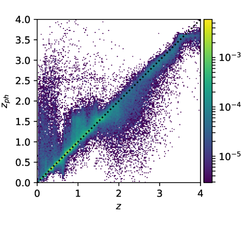
For realistic LSST photo-$z$ performance, we assess the impact of unmodelled realistic photo-$z$ errors and the uncertainties in the shape of $\hat{n}^{i}(z)$ on inferred cosmological parameters. For the latter case, we approximate $n^{i}_{\rm true}(z)$ with $n^{i}_{\rm ph}(z)$ after removing centroid bias. We use the Tomographic dataset and model photo-$z$ performance with a recently simulated spectroscopic calibration sample, employed by Rhodes et al. (2017). Figure 2 illustrates this dataset. To capture the photo-$z$ performance of the LSST filter set, the dataset was constructed by applying a basic template-based method to the COSMOS catalogue (Laigle et al., 2016). However, a variety of factors are not modelled, such as the dependence on depth, data, quality, or selection function (Rhodes et al., 2017).

As we discuss in detail in Appendix B, these photometric redshifts do not meet the LSST photo-$z$ requirements. Despite these drawbacks, it gives an estimate of LSST’s photo-$z$ PDF (i.e. $p(z_{\rm ph}|z)$, the probability density function for measuring a photo-$z$ value at a given spectroscopic redshift), and will suffice for assessing the relative resilience of $n_{\rm pk}$ and $P^{\kappa\kappa}$ to these types of photo-$z$ errors.

To simulate photo-$z$ errors, we divide the simulated spectroscopic calibration sample into 40 uniform bins spanning $0<z_{\rm ph}<3$; each bin contains at least 987 galaxies. Within each photo-$z$ bin, we compute normalised histograms of $e_{z}\equiv\frac{z_{\rm ph}-z}{1+z}$ with the number of bins given by the Freedman–Diaconis Estimator (Freedman & Diaconis, 1981). For simplicity, we assume that these histograms perfectly describe the distribution of photo-$z$ errors and that $p\left(e_{z}|z_{\rm ph}\right)$ is the same for both the simulated calibration set and our simulated survey.

To assess the impact of unmodelled realistic errors we randomly draw the true source redshift $z$ for each galaxy in $\hat{{\boldsymbol{\gamma}}}_{\rm obs}({\boldsymbol{\theta}}_{g},z_{g})$ from $p\left(e_{z}|z_{\rm ph}\right)$ when we set $z_{\rm ph}$ to $z_{g}$. We then perform ray-tracing simulations to produce new $\hat{{\boldsymbol{\gamma}}}_{\rm obs}({\boldsymbol{\theta}}_{g},z_{g})$. Each realisation of $\hat{{\boldsymbol{\gamma}}}_{\rm obs}({\boldsymbol{\theta}}_{g},z_{g})$ uses a different random seed to draw true source redshifts. All randomly drawn values falling outside of $0\leq z\leq 4.1925$ are set to the closest value in the range; $z=4.1925$ is slightly smaller than the redshift of the furthest lens plane in our Tomographic dataset. Figure 11 below shows a comparison between $n_{\rm ph}(z)$ and the average $n_{\rm true}(z)$.

To assess the impact of errors in the shape of $\hat{n}^{i}(z)$, we follow the same procedure outlined in the preceding paragraph with a modification. After producing the source redshifts for a given realisation, we remove the centroid bias between $n^{i}_{\rm true}(z)$ and $n^{i}_{\rm ph}(z)$ from the source redshifts of the galaxies in bin $i$ before performing ray-tracing. In other words, we modify $n^{i}_{\rm true}(z)$ to be equal to $n^{i}_{\rm true}(z+\delta z^{i})$. This approach is equivalent to assuming that a calibration process was able to obtain the correct centroid of the redshift-distribution in each tomographic bin. We believe this is a reasonable approximation for setting $\hat{n}^{i}(z)=n^{i}_{\rm ph}(z-\delta z^{i})$; in any case it allows us to isolate errors arising purely from differences in the shapes of $n^{i}_{\rm true}(z)$ and $\hat{n}^{i}(z)$.

Figure 3: Illustration of the calculation of the figure-of-merit for the parameter bias, $\mathcal{B}/\mathcal{U}$. The black star and contour indicate the most likely $\Lambda$CDM cosmology ($\hat{\bf p}_{unbiased}$) and $68\%$ confidence contour inferred from the tomographic $n_{\rm pk}(\nu)$ without photo-$z$ errors. The red star indicates the most-likely value inferred with photo-$z$ bias, given by $b_{\rm ph}(z)=b(1+z)$ with $b=-0.009$. $\mathcal{B}/\mathcal{U}$ is the ratio between the lengths of the solid red line (the magnitude of parameter bias and the blue dotted line (the distance from $\hat{\bf p}_{unbiased}$ to the unbiased $68\%$ confidence contour along the direction of parameter bias).

2.5 Cosmological Parameter Inference

Table 3: Brief summary of cosmological models and the maximum survey size (above which we can no longer reliably measure the parameter biases $\mathcal{B}/\mathcal{U}$; see § 2.5.1) for the two summary statistics we employ: peak counts ($n_{\rm pk}$) and tomographic power spectrum ($P^{\kappa\kappa}$). For the latter, we employ a principal component analysis (PCA) and keep $N_{c}=30$ components (see § 2.5.3).

model	${\bf p}$	Points in $\chi^{2}$ grid	$\Omega_{max}$ ($\rm{deg}^{2}$)
			$n_{\rm pk}$	$P^{\kappa\kappa}(N_{c}=30)$
$\Lambda$CDM	$(\Omega_{m},\sigma_{8})$	$1000^{2}$	984	15033
$w$CDM	$(\Omega_{m},w,\sigma_{8})$	$100^{3}$	2002	24930

Bayes’ theorem allows us to synthesise the posterior probability distribution of $\hat{\bf p}$, assuming some model $M$, from an observed summary statistic vector $\hat{\bf d}^{obs}$ and prior knowledge $p({\bf p}|M)$ using

$$p({\bf p}|\hat{\bf d}^{obs},M)=\frac{p(\hat{\bf d}^{obs}|{\bf p},M)p({\bf p}|M)}{p(\hat{\bf d}^{obs}|M)}.$$ (8)

In this equation, $p(\hat{\bf d}^{obs}|M)$ gives the probability of observing $\hat{\bf d}^{obs}$ for any cosmology while $p(\hat{\bf d}^{obs}|{\bf p},M)$ is the likelihood function for observing $\hat{\bf d}^{obs}$ in cosmology ${\bf p}$. We infer the posterior of $\hat{\bf p}$ using two separate cosmological models: $\Lambda$CDM and $w$CDM. Tables 1 and 3 list details about inference in each model.

For our analysis, we treat $p({\bf p}|M)$/$p(\hat{\bf d}^{obs}|M)$ as a normalisation constant within the region sampled by $\{{\bf p_{i}}\}$ and zero elsewhere. We assume that our summary statistics follow a multivariate Gaussian distribution with covariance matrix ${\bf{C}}$. Thus, ${\rm log}\ p({\bf p}|\hat{\bf d}^{obs},M)\propto-\chi^{2}(\hat{\bf d}^{obs}|{\bf d}({\bf p}),{\bf C})$, where

$$\chi^{2}(\hat{\bf d}^{obs}|{\bf d}({\bf p}),{{\bf C}})=(\hat{\bf d}^{obs}-{\bf d}({\bf p}))^{T}{{\bf C}^{-1}}(\hat{\bf d}^{obs}-{\bf d}({\bf p})).$$ (9)

We assume that ${\bf C}$ is independent of cosmology, and estimate it using the $N_{r}$ realisations of the summary statistics $\hat{\bf d}_{r}$ computed for ${\bf p_{0}}$ with $\hat{\kappa}_{r}^{\rm fid}({\boldsymbol{\theta}}_{p})$ or $\hat{\kappa}_{r}^{\rm fid}({\boldsymbol{\theta}}_{p},\bar{z}_{b})$. The formula for the unbiased estimate of ${\bf C}$ is

$$\hat{\bf C}=\frac{1}{N_{r}-1}\sum_{r=1}^{N_{r}}(\hat{\bf d}_{r}-{\bf d}({\bf p}_{0}))(\hat{\bf d}_{r}-{\bf d}({\bf p}_{0}))^{T}.$$ (10)

To make the inverse of $\hat{\bf C}$ an unbiased estimator of ${\bf C}^{-1}$, we rescale it with

$$\hat{{\bf C}^{-1}}=\frac{N_{r}-N_{b}-2}{N_{r}-1}{\bf C}^{-1},$$ (11)

where $N_{b}$ is the number of components of the summary statistic (Hartlap et al., 2007).

To evaluate the likelihood function for a ${\bf p}$ not included in $\{{\bf p_{i}}\}$, we make use of cosmology interpolators. We follow Z16 for the Single-$z$ dataset and interpolate $\chi^{2}(\hat{\bf d}^{obs}|{\bf d}({\bf p}),\hat{{\bf C}})$ at an arbitrary cosmology ${\bf p}$ using the values at each cosmology in $\{{\bf p_{i}}\}$. However, unlike Z16, we use cubic interpolation rather than linear interpolation, as the latter will always identify a cosmology in $\{{\bf p_{i}}\}$ as the most-likely cosmology $\hat{\bf p}$. For the Tomographic dataset, we instead employ an emulator which interpolates ${\bf d}({\bf p})$ between each cosmology in $\{{\bf p_{i}}\}$ using augmented RBF interpolation with a cubic basis function (Petri, 2016). Our choice of interpolation differs from that of P16 and we refer the reader to Appendix C for a comparison of various interpolation schemes.

Since we only infer $2-3$ cosmological parameters, we perform inference by sampling a grid using the interpolator. Hereafter we refer to that grid as the sampled $\chi^{2}$ grid. Tables 1 and 3 provides details about the sampling of these grids.

Our assessment of the impact of unmodelled photo-$z$ errors and of the errors in the shape of $n^{i}(z)$ requires a different approach. In both cases, $n_{\rm true}(z)$ is randomly drawn for each realisation, yielding different values of ${\bf d}$. Consequently, we adopt the basic procedure of constructing separate grids of $\chi^{2}$ values for each realisation. Then for each point on the grid, we average the $\chi^{2}$ values over all $N_{r}$ realisations.

2.5.1 Quantifying Inferred Parameter Biases

Any discrepancies between $\hat{n}(z)$ and $n_{\rm true}(z)$ will lead to biases on $\hat{\bf p}$. We can debias the results by propagating the uncertainties in $\hat{n}(z)$ to $\hat{\bf p}$ (e.g. Huterer et al., 2006; Abbott et al., 2016). Unfortunately, this is computationally prohibitive for non-analytic statistics, like peak counts because it requires rebuilding the interpolator (and all of the ray-tracing simulations) for every sampled $\hat{n}(z)$. To circumvent this cost in their analysis of DES SV data using scaled peaks counts, Kacprzak et al. (2016) parameterised the linear impact that the centroid bias of the entire galaxy distribution (they didn’t use tomography) had on the heights of the scaled peaks. For our analysis, we choose not to directly propagate the uncertainty.

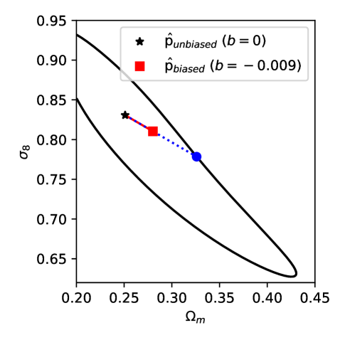
Instead, we define a bias-to-uncertainty ratio $\mathcal{B}/\mathcal{U}$, as the ratio of the magnitude of the bias $|\Delta{\bf p}|\equiv|\hat{\bf p}_{biased}-\hat{\bf p}_{unbiased}|$ and the distance between the unbiased most-likely $\hat{\bf p}$ and the unbiased $68\%$ confidence contour along the direction of the bias $|\Delta{\bf p}|$. Figure 3 presents a graphical illustration of $\mathcal{B}/\mathcal{U}$ for tomographic $n_{\rm pk}(\nu)$ in a case with uncorrected photo-$z$ bias. The above definition is necessary, because the posteriors can change their shapes due to discrepancies between $\hat{n}(z)$ and $n_{\rm true}(z)$. $\mathcal{B}/\mathcal{U}$ is defined such that its value is independent of the relative normalisation of the different components of ${\bf p}$.

We employ $\mathcal{B}/\mathcal{U}$ as a proxy for the degradation in the constraints since the degraded posterior needs to include both the biased and unbiased most likely values of $\hat{\bf p}$. As we scale our survey to larger sizes, and the posterior more closely resembles a symmetric Gaussian, $\mathcal{B}/\mathcal{U}$ becomes a better proxy for posterior degradation. We identify the case where $\mathcal{B}/\mathcal{U}=1.5$ as the benchmark for when photo-$z$ errors contribute considerable uncertainty to the inferred $\hat{\bf p}$. This value corresponds to an error degradation of $\sim 50\%$, which is analogous to the benchmark employed by Huterer et al. (2006) while measuring degradations in marginalised uncertainties.

2.5.2 Scaling Survey Size

To directly compare our results from the Tomographic dataset to a large survey such as LSST, we need to scale our $\chi^{2}$ values to be consistent with a survey subdivided into $N$ $(3.36{\rm deg})^{2}$ subfields. To do this we assume that our subfield is an average subfield in the survey, and we multiply all of the $\chi^{2}$ values in the sampled grid by a factor of $N$.

The finite number of cosmologies in $\{{\bf p_{i}}\}$ introduces error to the interpolated ${\bf d}({\bf p})$ that will propagate to errors in the computed $\chi^{2}$ value. For each summary statistic, we compute the average magnitude of this propagated interpolation error, by identifying the 10 closest values in $\{{\bf p_{i}}\}$ to the most likely $\hat{\bf p}$ and employing

$$\frac{1}{10}\sum_{j=1}^{10}\left|\frac{\chi^{2}(\hat{\bf d}^{obs}|{\bf d}({\bf p}_{j}),\hat{{\bf C}})-\chi^{2}(\hat{\bf d}^{obs}|\hat{\bf d}({\bf p}_{j}),\hat{{\bf C}})}{\chi^{2}(\hat{\bf d}^{obs}|{\bf d}({\bf p}_{j}),\hat{{\bf C}})}\right|,$$ (12)

where $\hat{\bf d}({\bf p}_{j})$ is emulated from $\{{\bf p_{i}}\}$ excluding ${\bf p}_{j}$.

This interpolation error corresponds to a maximum survey size for which we can reliably compute $\mathcal{B}/\mathcal{U}$. This is because as the survey is scaled up, the $\chi^{2}$ values increase, the $68\%$ confidence contour shrinks, and it eventually corresponds to a small region that is buried in the numerical noise in the $\chi^{2}$ surface. Unless the difference between $\chi^{2}_{\rm min}$ and the $\chi^{2}$ value corresponding to the $68\%$ confidence contour is larger than the numerical interpolation error, we can not reliably measure the distance between the most-likely $\hat{\bf p}$ and the contour. Table 3 lists this maximum survey size for each cosmological model and summary statistic.

In addition to numerical limits on computing the bias $\mathcal{B}/\mathcal{U}$, the original $\chi^{2}$ grid can also become too poorly sampled to reliably infer the posterior for large $N$ in the $w$CDM cosmology. These cases are identified when the marginalised standard deviation of a component $\hat{\bf p}$ is smaller than the sampling resolution in that component. When these cases arise, we simply resample the grid with $101^{3}$ grid points centred on the original most-likely $\hat{\bf p}$ and spaced with resolutions at least half the size of the marginalised standard deviations. Because of the slightly higher resolution grid, the most likely-value $\hat{\bf p}$ may shift. For consistency, we always compute the $\mathcal{B}/\mathcal{U}$ for a given statistic in a $w$CDM cosmology with respect to the $\hat{\bf p}$ with the lowest unscaled $\chi^{2}$ value encountered on any grid.

Our assessment of biases in $\hat{\bf p}$ that arise from errors in the shapes of $n^{i}(z)$ involves a slightly modified procedure. To construct a survey of $N$ subfields, we group the $N_{r}=1000$ realisations into as many independent groups of $N$ realisations as possible without having any realisations repeat groups and discard all remaining realisations not assigned to a group. Then when adjusting the randomly drawn values of $n^{i}_{\rm true}(z)$ before ray-tracing, we use a single correction value for all realisations in a given group that removes the centroid bias between the group’s combined $n^{i}_{\rm ph}(z)$ and $n^{i}_{\rm true}(z)$. For a survey of $N>1$ subfields, this allows the $n^{i}_{\rm ph}(z)$ in individual subfields to still have centroid bias, which then cancel out when these individual subfields are aggregated. Consequently, our assessment of the impact of errors in the shape of $n^{i}(z)$ in surveys of size $N$ effectively includes ${\rm floor}(1000/N)$ unique realisations of the survey produced from ${\rm floor}(1000/N)\times N$ realisations of $\hat{{\boldsymbol{\gamma}}}_{\rm obs}({\boldsymbol{\theta}}_{g},z_{g})$.

2.5.3 Principal Component Analysis

As in P16, we attempt to apply Principal Component Analysis (PCA) to reduce the dimensionality of the summary statistics in the Tomographic dataset. This is necessary because, as mentioned above, the full power spectrum has 825 components, which is $\sim 5\%$ of the $N_{r}=16,000$ realisations used to construct the emulator and covariance matrix. As a first step, we compute the mean $\langle{\bf d}\rangle$ and the variance $\sigma_{\bf d}$ of each statistic, over all cosmologies in $\{{\bf p_{i}}\}$. We then follow the procedure in P16, except for one difference. While the PCA in P16 is performed on the normalised components $[d_{i}-\langle{\bf d}_{i}\rangle]/\langle{\bf d}_{i}\rangle$, we instead use the whitened components $[d_{i}-\langle{\bf d}_{i}\rangle]/\sigma({\bf d_{i}})$. Consequently, in our case, each component has unit variance before applying PCA (Ivezić et al., 2014), although they still have co-variance.

We refer the reader to Appendix D for a detailed explanation for our choices of the number of principal components $N_{c}$ for each statistic. We ultimately choose not to use PCA for the $n_{\rm pk}$ (equivalent to $N_{c}=100$) and to use $N_{c}=30$ for $P^{\kappa\kappa}$. Table 3 lists the maximum survey sizes for which we can compute $\mathcal{B}/\mathcal{U}$ using $P^{\kappa\kappa}$ with $N_{c}=30$ components and the peak counts using the full set of components.

Figure 4: Comparisons between the average peak count histograms in the fiducial cosmology with and without a constant photo-$z$ bias $b_{\rm ph}$ (left panel), and of a different cosmology $(\Omega_{m},\sigma_{8})=(0.259,0.875)$ with $b_{\rm ph}=0$ (right panel). The cosmology in the right comparison was selected because it has a similar $\Sigma_{8}$ value to the most likely $\Sigma_{8}$ from the average peak histogram in the fiducial cosmology with a bias of $b_{\rm ph}=-0.086$. This side-by-side comparison qualitatively illustrates how $b_{\rm ph}$, in our simple case, creates deformations in the peak count histogram that can be mimicked by cosmologies with a higher $\Sigma_{8}$. (Note that we use 50 bins in this figure for clarify of presentation; in the calculations we use a finer binning with 100 bins.)

Table 4: The table shows the biased inferred best-fit $\Sigma_{8}$ values for source planes at various biased redshifts. We also list the reduced $\chi^{2}$ value for the best-fit cosmology using the average peak histogram.

$b_{\rm ph}$	$\Sigma_{8}^{(a)}$	reduced $\chi^{2}{}^{(b)}$	$\left<\Sigma_{8}^{r}\right>$	median$\{\Sigma_{8}^{r}\}$	std$\{\Sigma_{8}^{r}\}$
$-0.233$	0.946	$+0.00352$	0.929	0.926	0.0421
$-0.183$	0.912	$+0.00282$	0.906	0.905	0.0402
$-0.134$	0.893	$+0.00221$	0.880	0.880	0.0397
$-0.086$	0.866	$+0.00279$	0.856	0.857	0.0397
$-0.040$	0.832	$-0.00006$	0.831	0.829	0.0362
0	0.8	0	0.809	0.799	0.0296
$+0.005$	0.797	$-0.00385$	0.808	0.798	0.0306
$+0.049$	0.787	$+0.00263$	0.787	0.787	0.0334
$+0.092$	0.766	$-0.00092$	0.764	0.767	0.0371
$+0.135$	0.756	$+0.00026$	0.740	0.745	0.0399
$+0.176$	0.706	$-0.00303$	0.715	0.714	0.0413
$+0.216$	0.683	$-0.00443$	0.686	0.693	0.0454

^a The most likely $\Sigma_{8}$ for the average peak histogram
^b Negative values are an artifact of the interpolation of $\chi^{2}$ values.

Figure 5: $95.5\%$ parameter confidence contours inferred for the fiducial cosmology when the source plane is placed at redshifts $z$ biased by various constant values of $b_{\rm ph}$. The black star indicates the true cosmology. As this plot illustrates, the impact of a constant photo-$z$ bias is to shift the contours perpendicular to the degenerate direction.

Figure 6: The parameter bias ($\delta\Sigma_{8}$) as a function of constant photo-$z$ bias ($b_{\rm ph}$). We compute $\delta\Sigma_{8}$ using the median($\Sigma_{8}^{r}$) of the best fits over all realisations of the mock observations. The error-bars, obtained from std$(\Sigma_{8}^{r})$, are smaller than the markers. The red dashed line illustrates the least squares error-weighted best fit line, given by $\delta\Sigma_{8}=(0.5211\pm 0.0002)b_{\rm ph}+(0.01020\pm 3\times 10^{-5})$

Figure 7: The $95.5\%$ confidence contours for the tomographic $n_{\rm pk}(\nu)$ (left column) and $P^{\kappa\kappa}(l)$ (right column) for different small biases parameterised by $b$ in a $w$CDM cosmology. Each panel in the top (bottom) row shows the contours for the posteriors marginalised over $w$ ($\sigma_{8}$). The black star shows the fiducial cosmology used to generate the observations.

Figure 8: Same as Fig. 7, except that we have scaled the likelihood values to those of a survey made up of $N=177$ subfields ($\sim 2000~{}{\rm deg}^{2}$). In this figure, stars mark the most-likely values inferred either from peak counts or from the power spectrum.

Figure 9: Figure of merit $\mathcal{B}/\mathcal{U}$ for the bias resulting from photo-$z$ errors parameterised by constant values of bias parameter $b$. $\mathcal{B}/\mathcal{U}$ is the size of the bias in the inferred cosmological parameters, relative to the distance between the unbiased most likely value to the $68\%$ confidence contour, along the direction of the bias. The horizontal dashed line indicates where this ratio has a value of 1.5 (our proxy for degrading the constraints by $~{}50\%$). The top (bottom) row shows $\mathcal{B}/\mathcal{U}$ in a $\Lambda$CDM ($w$CDM) cosmology, and the left (right columns) are for peaks (power spectrum). The colors and shapes of the markers correspond to different bias parameters $b$ as labelled. The vertical gray line marks the maximum scaled up survey size for which our results can be trusted (points to the right of this line may have significant interpolation errors).

Figure 10: Maximum survey size for which photo-$z$ biases parameterised with constant parameter $b$ produce tolerable error degradations. The lines on this plot roughly trace out the survey sizes for which the parameter bias is $50\%$ larger than the distance to the $68\%$ confidence contour from the most-likely value along the direction of the bias. The four curves correspond to $\Lambda$CDM and $w$CDM parameter inferences from $n_{\rm pk}$ and $P^{\kappa\kappa}$, as labelled.

3 Results

3.1 Residual photo-$z$ Bias

This work primarily focuses on the impact of residual photo-$z$ bias on $\hat{\bf p}$. For discussions of our motivation and how we model residual $b_{\rm ph}$, we refer to the reader back to § 2.4.1. However, we remind the reader that each galaxy’s spectroscopic redshift is given by its photo-$z$ subtracted by $b_{\rm ph}$. We divide our assessment of $b_{\rm ph}$ into two parts. First, we study a single source redshift and a simple constant $b_{\rm ph}$ to build our intuition. We then analyse a more realistic case involving tomography and an LSST-like $n_{\rm ph}(z)$.

3.1.1 Single-$z$ dataset: photo-$z$ Biases

We begin with the Single-$z$ dataset. The true distribution of galaxies and estimate are given by $n_{\rm true}(z)=25~{}{\rm arcmin}^{-2}\delta(z-1+b_{\rm ph})$ and $\hat{n}(z)=25~{}{\rm arcmin}^{-2}\delta(z-1)$. Table 4 lists the values of $b_{\rm ph}$ we used. All values, other than $b_{\rm ph}=0$, were selected such that each source plane lies just behind a lens plane.

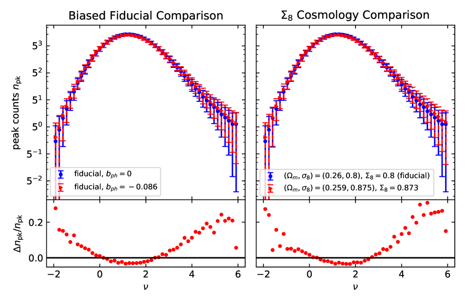
The left column of Figure 4 illustrates the impact of a bias $b_{\rm ph}\neq 0$ on the peak counts in the fiducial model. The top panel shows $n_{\rm pk}$ in the unbiased ($b_{\rm ph}=0$; blue dots), and a biased ($b_{\rm ph}=-0.086$; red triangles) case. The bottom panel shows the fractional difference $[n_{\rm pk}(b_{\rm ph}=-0.086)-n_{\rm pk}(b_{\rm ph}=0)]/n_{\rm pk}(b_{\rm ph}=0)$.

The lower left panel of Figure 4 shows that outside of $0\la\nu\la 2.5$, the fractional bias in the number of peaks is proportional to $|\nu|$. For $2.5\la\nu\leq 4.1$, this finding is in qualitative agreement with that of Kacprzak et al. (2016) for shear peaks. Although our respective findings differ for the number of peaks with $0\leq\nu\la 2.5$, we attribute this to the fact that Kacprzak et al. (2016) examined relative differences in the numbers of peaks after correcting for peaks contributed by noise (which dominate at lower $\nu$), and that we each use different $n_{\rm true}(z)$ and filter scales.

We next contrast these changes in the peak counts with those introduced by changes in cosmology. To this end, we define a quantity often used to parameterise the degeneracy between $\Omega_{m}$ and $\sigma_{8}$,

$$\Sigma_{8}\equiv\sigma_{8}\left(\frac{\Omega_{m}}{0.26}\right)^{\alpha}.$$ (13)

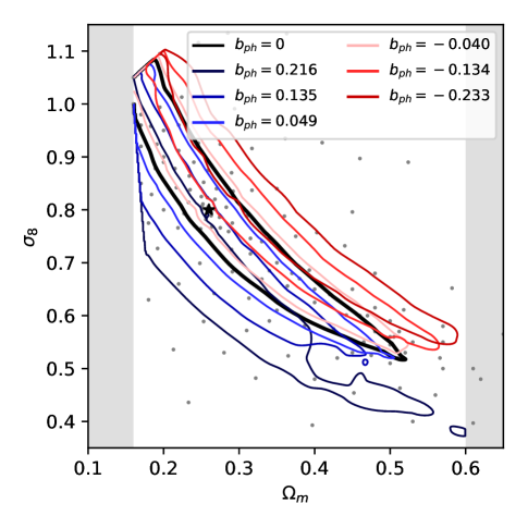
We set $\alpha=0.59$ because it yields the most tightly constrained combination (for $b_{\rm ph}=0$) using the procedure outlined in Petri et al. (2015). The right panel in Figure 4 shows how $n_{\rm pk}$ is modified in a cosmology with a higher $\Sigma_{8}$. This cosmology was selected because it is among the $\{{\bf p_{i}}\}$ with the three closest $\Sigma_{8}$ values to the best-fit value of the biased fiducial case (shown in the left panel), and it has the most similar $(\Omega_{m},\sigma_{8})$ to the fiducial values. The side-by-side comparison of the left vs. right panels illustrates that a negative $b_{\rm ph}$ causes changes in $n_{\rm pk}$ that closely resemble the changes arising from modifying $\Sigma_{8}$. This means that a negative $b_{\rm ph}$ induces changes to $n_{\rm pk}$ similar to seeing a universe with more evolved structure.

Figure 5 displays the $95.5\%$ confidence contours of the inferred posteriors of $\hat{\bf p}$ for a subset of $b_{\rm ph}$ values. The figure illustrates that a positive (negative) $b_{\rm ph}$ shifts the posterior to the lower left (upper right) corner of the figure, perpendicular to the direction of degeneracy, as expected from Figure 4.

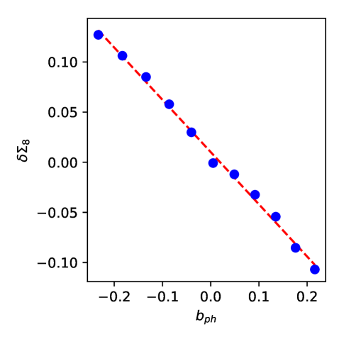
Because the contours largely retain their shape and only shift perpendicular to the direction of degeneracy, we can quantify the impact of $b_{\rm ph}$ on $\hat{\bf p}$ by measuring the displacement of the curve running along the direction of degeneracy, in the direction perpendicular to the curves with $\Sigma_{8}=$constant. For each value of $b_{\rm ph}$, we compute the biased value of $\Sigma_{8}$ by plugging the most-likely $\Omega_{m}$ and $\sigma_{8}$ into Equation 13.

For each $b_{\rm ph}$, Table 4 lists the $\Sigma_{8}$ and corresponding $\chi^{2}$ values inferred from the $n_{\rm pk}(\nu)$, averaged over all 500 realisations of $\hat{\kappa}_{\rm obs}({\boldsymbol{\theta}}_{p})$. Note that the negative $\chi^{2}$ arise from our use of cubic interpolation. We also list the corresponding averages, medians, and standard deviations ($\langle\Sigma_{8}^{r}\rangle$, median$\{\Sigma_{8}^{r}\}$, std$\{\Sigma_{8}^{r}\}$) of the $\Sigma_{8}$ values fit in each individual realisation of $\hat{\kappa}_{\rm obs}({\boldsymbol{\theta}}_{p})$.

Figure 6 displays the linear relationship between $\delta\Sigma_{8}$, the bias in the posterior, and $b_{\rm ph}$. We find the best-fit, when the $\delta\Sigma_{8}$ is defined as the median$(\Sigma_{8}^{r})$ over all realisations. The best-fit line is given by $\delta\Sigma_{8}=(0.5211\pm 0.0002)b_{\rm ph}+(0.01020\pm 3\times 10^{-5})$. The non-zero $y$-intercept is artificial, and we believe that it can be explained by the limitations of our experiment. With more finely sampled cosmologies $\{{\bf p_{i}}\}$, lens planes, and $b_{\rm ph}$’s, the $y$-intercept should approach zero.

The above results can be interpreted intuitively as follows. If we incorrectly assign lower redshifts to galaxies, we will be measuring stronger lensing for this apparent redshift than we should be (since the galaxies are farther away than we think). As a result, we will be misled into thinking that our universe has a higher $\Sigma_{8}$ – because in that case, the universe would have more evolved structure today, causing a stronger lensing.

3.1.2 Tomographic dataset: residual photo-$z$ biases

Having built up basic intuition, we next assess the impact of $b_{\rm ph}$ on parameters inferred using tomography for a mock survey with an LSST-like $n_{\rm ph}(z)$ using the Tomographic dataset.

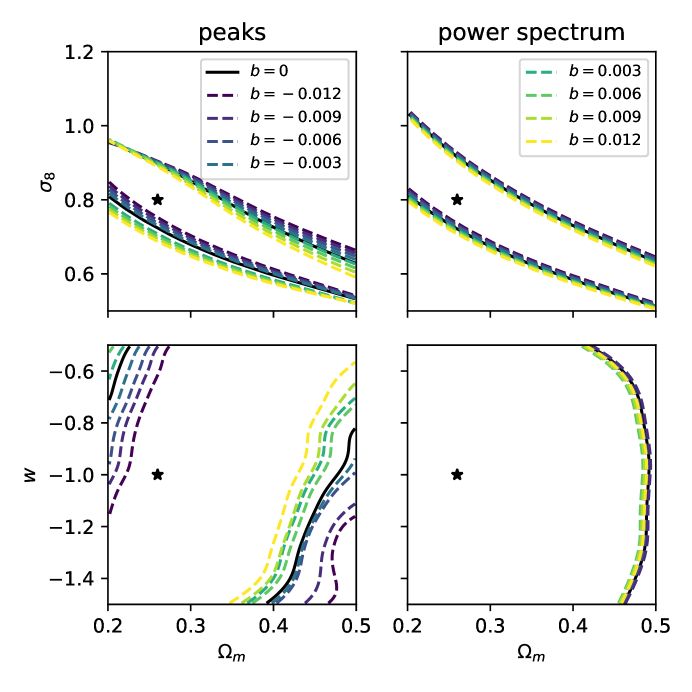
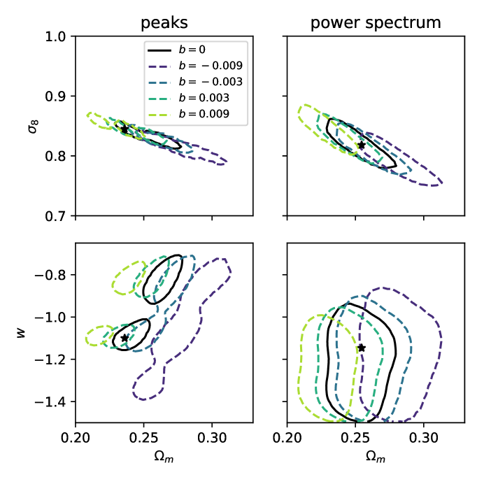
Figure 7 shows the $95.5\%$ confidence contours inferred for a $w$CDM cosmology from $n_{\rm pk}$ (left column) and from $P^{\kappa\kappa}$ (right column) from mock observations of a single subfield with bias parameter $b$ values of $\pm 0.003$, $\pm 0.006$, $\pm 0.009$, and $\pm 0.012$. Figure 8 is identical except that the contours are shown for a subset of the $b$ values for a scaled survey including $N=177$ subfields ($\sim 2000~{}{\rm deg}^{2}$). The confidence contours for the scaled posteriors are equivalent to high likelihood regions of the unscaled posteriors. In both figures, the confidence contours in the top (bottom) row are drawn for posteriors marginalised over $w$ ($\sigma_{8}$), and are clipped due the finite extent of our non-zero uniform prior.

The shifts in the unscaled $95\%$ confidence contours in both the ($\Omega_{m},\sigma_{8}$) and ($\Omega_{m},w$) planes are smaller for $P^{\kappa\kappa}$ than for $n_{\rm pk}$. While the changes in the unscaled ($\Omega_{m},\sigma_{8}$) contours inferred with $P^{\kappa\kappa}$ are similar to the shifts discussed in § 3.1.1 for the Single-$z$ dataset, the changes in the contours inferred from $n_{\rm pk}$ are more complex and include noticeable deformations in the overall shape. We believe that this more complex behavior can be explained by the tomographic information breaking the degeneracy between $b_{\rm ph}$ and $\Sigma_{8}$. Such an explanation only works for redshift-dependent $b_{\rm ph}$.

At the same time, the ($\Omega_{m},\sigma_{8}$) contours in Figure 8 from both statistics shift along the direction of degeneracy. Positive (negative) $b_{\rm ph}$ shifts these contours towards more negative (positive) $\Omega_{m}$ and slightly decreases (increases) the enclosed area. The shifts in the ($\Omega_{m},w$) contours due to small, positive (negative) $b_{\rm ph}$ for each statistic in Figures 7 and 8 are consistent with the entire unscaled posterior shifting coherently toward negative (positive) $\Omega_{m}$; they also cause the scaled up contour to contract (expand).

We also briefly discuss the effects of $b_{\rm ph}$ on the unscaled $95.5\%$ confidence contour in the ($\Omega_{m},\sigma_{8}$) plane when $b=\pm 0.025,$ $\pm 0.05$, and $+0.1$. These contours have been omitted from Figure 7 but are shown in Figure 20 of Appendix E. For galaxies with $z_{\rm ph}=1$, these $b_{\rm ph}$ are of similar magnitudes to those assessed in § 3.1.1. At these larger $|b_{\rm ph}|$, we find a sharp departure in the behavior of the $n_{\rm pk}$ contours. These contours display larger shifts in the $\Omega_{m}$ direction, more significant shape deformation, and less smooth overall dependence on $b$. In contrast, the shifts in the $P^{\kappa\kappa}$ contours are consistent with proportionally larger magnitude shifts along the direction of degeneracy that the shifts illustrated in Figure 7.

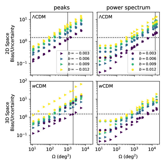
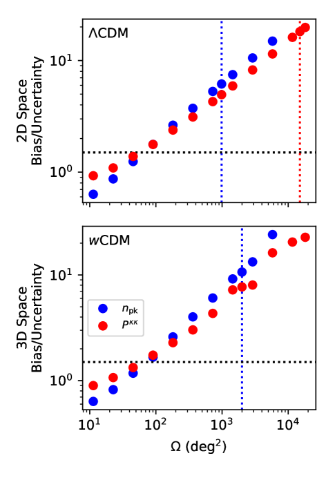
Figure 9 shows the dependence of the relative bias figure of merit $\mathcal{B}/\mathcal{U}$ (defined in the previous section) on $\Omega$, the number of subfields in a scaled up survey, and the bias parameter $b$. Because of the weak sensitivity of either statistic to $w$, we primarily focus on $\mathcal{B}/\mathcal{U}$ for inference in $\Lambda$CDM cosmologies (top row). For completeness, Figure 9 also includes the $\mathcal{B}/\mathcal{U}$ for $w$CDM cosmologies (bottom row). Data for $n_{\rm pk}$ ($P^{\kappa\kappa}$) are displayed in the left (right) column. The vertical gray lines indicate $\Omega_{\rm max}$, the largest $\Omega$ for which we can reliably forecast $\mathcal{B}/\mathcal{U}$ (see § 2.5.2), and the horizontal dashed lines mark our 50% benchmark for significant posterior degradation (see § 2.5.1). Any error in the estimation of the most-likely $\hat{\bf p}$ due to the finite sampling of the inference grid is small and only relevant to $\mathcal{B}/\mathcal{U}$ for $|b|\sim 0.003$ due to the small absolute size of the bias in $\hat{\bf p}$.

There are two salient points revealed by Figure 9. First, for large $\Omega$, the $\mathcal{B}/\mathcal{U}$ of each summary statistic roughly follows a power-law $\mathcal{B}/\mathcal{U}\propto\Omega^{1/2}$. Such behavior is expected at large $\Omega$ because the posterior should resemble a Gaussian. Although such resemblance is not apparent in Figure 8 for a $w$CDM cosmology with $\Omega=2002~{}{\rm deg}^{2}$, it is evident for the contours of $\Lambda$CDM with $\Omega=984~{}{\rm deg}^{2}$. The other takeaway is that the uncertainty in $\hat{\bf p}$ is degraded by $\ga 50\%$ at smaller survey sizes for $n_{\rm peak}$ than for $P^{\kappa\kappa}$.

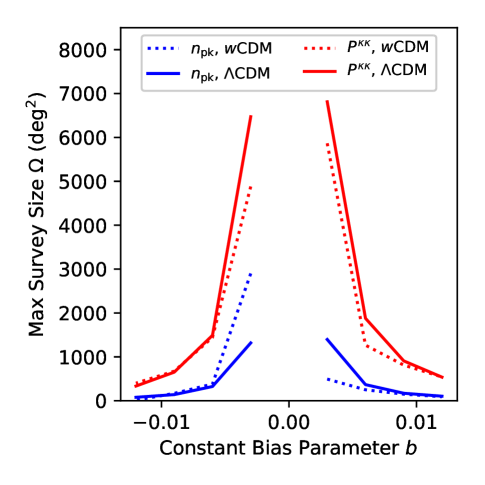
Figure 10 summarises the survey area $\Omega$ at which a given $b$ degrades the uncertainty in $\hat{\bf p}$ by $\sim 50\%$. To construct the figure, we use linear interpolation and extrapolation, in log-log space, using the points from Figure 9 to determine the survey sizes for which $\mathcal{B}/\mathcal{U}=1.5$. With the exception of the inference of a $w$CDM cosmology with $n_{\rm peak}$ when $b=-0.003$, we exclusively use data satisfying $\Omega\leq\Omega_{\rm max}$. For that particular case, we use the interpolated value between $\Omega=2002~{}{\rm deg}^{2}$ and $\Omega=2896~{}{\rm deg}^{2}$ because it yields a more conservative and realistic result.

The main conclusion from this last figure is that a residual bias $b_{\rm ph}$ with $|b|=0.003$ degrades $\Lambda$CDM parameter estimates for surveys with $\Omega\ga 1300\ {\rm deg}^{2}$ ($\ga 6500\ {\rm deg}^{2}$) when using $n_{\rm peak}$ ($P^{\kappa\kappa}$). For $w$CDM, the corresponding limits are $\Omega\ga 490\ {\rm deg}^{2}$ ($\ga 4900\ {\rm deg}^{2}$). It is worth noting that this effectively corresponds to a pessimistic “worst case scenario”: It is highly unlikely that the residual $b_{\rm ph}$ would match the upper limit of the LSST photo-$z$ requirements and have the same sign at all $z$.

Finally, one may ask if the presence of bias can be discovered from poor goodness-of-fit values. We find that the reduced $\chi^{2}$ values are much smaller than unity in all cases discussed in this section, except for peak counts at the largest bias ($b=0.1$, yielding reduced $\chi^{2}=0.66$), indicating that the biased best-fit models remain good fits to the mock data.

3.2 Realistic photo-$z$ Errors

In this subsection, we shift our focus to assessing the biases in $\hat{\bf p}$ induced by directly approximating $n_{\rm true}(z)$ with some variation of $n_{\rm ph}(z)$. We begin by investigating the impact of unmodelled photo-$z$ errors, the errors from simply setting $\hat{n}(z)=n_{\rm ph}(z)$. We then examine the impact of errors in the shape of $n^{i}_{\rm ph}(z)$ relative to the shape of $n^{i}_{\rm true}(z)$ in the absence of centroid bias. The latter case assumes that in each tomographic bin, a calibration process successfully. adds a constant to $n^{i}_{\rm ph}(z)$ to make its centroid match that of $n^{i}_{\rm true}(z)$. We remind the reader that for these assessments, we adopt the photo-$z$ PDF from a simulated calibration set taken from Rhodes et al. (2017). This simulated dataset accounts for LSST’s photometric filters and uses a basic spectral template to obtain photo-$z$’s, but does not meet the LSST science requirements (see Appendix B).

The un-optimised performance of the simulated photo-$z$ PDFs we adopted and our heavy reliance on photo-$z$ point estimates make the results conservative. Setting $\hat{n}(z)$ equal to the distribution of point estimates, rather than computing it like a real surveys (e.g. stacking redshift posteriors), makes our $\hat{n}(z)$ worse estimates of $n_{\rm true}(z)$ than those in real surveys. Furthermore, performing ray-tracing with these point estimates, instead of randomly drawing redshifts based on $\hat{n}^{i}(z)$, contrasts with how real surveys constrain cosmology with two-point statistics. This choice makes our results more sensitive to errors: even if $\hat{n}(z)$ were identical to the $n^{i}_{\rm true}(z)$, our results remain biased, since we do not assign the correct redshift to each galaxy. Consequently, our estimates in this subsection for the maximum survey sizes that avoid parameter degradation are conservative lower limits.

Figure 11: Illustrates the difference between the true galaxy redshift distribution (blue solid line) and the galaxy photo-$z$ distribution (dashed black line) entering our analysis. The true galaxy redshift distribution assumes that the spectroscopic calibration sample follows the same distribution as the surveyed galaxies.

Figure 12: $95.5\%$ confidence contours from lensing peaks (blue) and from the convergence power spectrum (red). The left column shows the unscaled contours while the right column shows the contours scaled to $N=177$ subfields ($\sim 2000~{}{\rm deg}^{2}$). The solid lines correspond to the unbiased case, and the dashed lines to the case where $n_{\rm true}(z)$ is approximated with $n_{\rm ph}(z)$ (i.e. ignoring photo-$z$ errors), computed with the photo-$z$ PDF estimated for LSST. The blue (red) points indicate the most likely cosmology inferred from $n_{\rm pk}$ ($P^{\kappa\kappa}$) in the absence of photo-$z$ errors.

Figure 13: Biases in the inferred parameters relative to the distance to the $68\%$ confidence contour along the direction of bias ($\mathcal{B}/\mathcal{U}$) as a function of scaled up survey size ($\Omega$). These biases are induced by approximating $n_{\rm true}(z)$ with $n_{\rm ph}(z)$ for simulated LSST photo-$z$ performance. The top (bottom) panel shows results for a $\Lambda$CDM ($w$CDM) cosmology, and the blue (red) markers for $n_{\rm pk}$ ($P^{\kappa\kappa}$). The horizontal black dotted line corresponds to significant degradation ($\mathcal{B}/\mathcal{U}$=1.5). The vertical blue (red) dotted lines indicate the maximum survey sizes above which numerical interpolation errors for $n_{\rm pk}$ ($P^{\kappa\kappa}$) invalidate our results.

Table 5: Summary of inferred cosmological parameter biases arising from taking photo-$z$ point estimates at face value and assuming $\hat{n}(z)$=$n_{\rm ph}(z)$. We list the reduced $\chi^{2}$ in each biased best-fit model, and the survey area $\Omega$ above which parameter estimates are degraded by $\geq 50\%$. The corresponding minimum average reduced $\chi^{2}$ value of the unbiased $\Lambda$CDM constraints from $n_{\rm peaks}$ ($P^{\kappa\kappa}$) is 1.53 (1.14). These values were computed by averaging the sampled $\chi^{2}$ grids over $N_{r}$ realisations.

model	$n_{\rm peaks}$		$P^{\kappa\kappa}(N_{c}=30)$
	reduced $\chi^{2}$	$\Omega$	reduced $\chi^{2}$	$\Omega$
$\Lambda$CDM	1.15226	$65.2\ {\rm deg}^{2}$	1.07622	$56.9\ {\rm deg}^{2}$
$w$CDM	1.16367	$73.2\ {\rm deg}^{2}$	1.11603	$61.6\ {\rm deg}^{2}$

3.2.1 Unmodelled photo-$z$ Errors

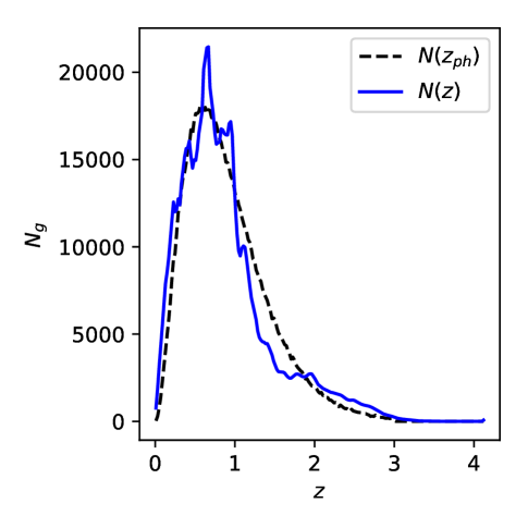
A simple way to frame the exercise in this subsection is that we are examining the cosmological-parameter degradation arising from entirely ignoring the photo-$z$ errors. Figure 11 illustrates both $n_{\rm ph}(z)$ (black dashed line) and the average true galaxy-redshift distribution $n_{\rm true}(z)$ (blue solid line).

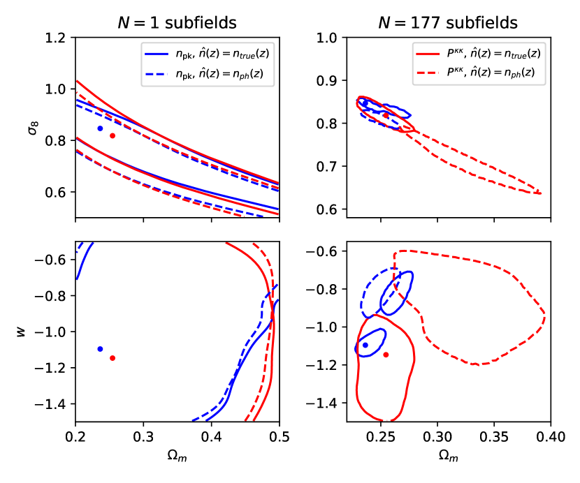
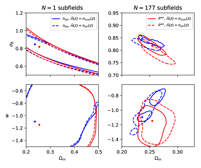
Figure 12 qualitatively shows the shifts in the $95.5\%$ confidence contours for a single subfield (left column) and a $\Omega=2002~{}{\rm deg}^{2}$ survey (right column), for $w$CDM parameters. We remind the reader that the right column equivalently shows very high likelihood regions of the unscaled subfield. The figure shows sets of contours assuming $\hat{n}(z)=n_{\rm ph}(z)$ (dashed lines) and $\hat{n}(z)=n_{\rm true}(z)$ (solid lines). The top (bottom) rows shows the $\Omega_{m}-\sigma_{8}$ ($\Omega_{m}-w$) contours marginalised over $w$ ($\sigma_{8}$). The blue (red) lines illustrate the confidence contours inferred from $n_{\rm pk}$ ($P^{\kappa\kappa}$).

Joint examination of the columns of Figure 12 indicate that the photo-$z$ errors induce a changes to the $\Omega_{m}-\sigma_{8}$ posterior, inferred with $n_{\rm pk}$ and marginalised over $w$, consistent with a coherent shift of the posterior towards negative $\sigma_{8}$. The change to the $\Omega_{m}-\sigma_{8}$ posterior for $P^{\kappa\kappa}$ is different; the unscaled contour shifts towards negative $\Sigma_{8}$ while the high likelihood contour shifts and expands along $\Sigma_{8}$. We also find that the $\Omega_{m}-w$ contour inferred with $n_{\rm pk}$ ($P^{\kappa\kappa}$), from a $\Omega=2002~{}{\rm deg}^{2}$ survey, shifts toward negative $\Omega_{m}$ (positive $\Omega_{m}$ and $w$). However, the changes to all $\Omega_{m}-w$ contours inferred from a single subfield, are ambiguous due to the large size of the contours compared to the prior.

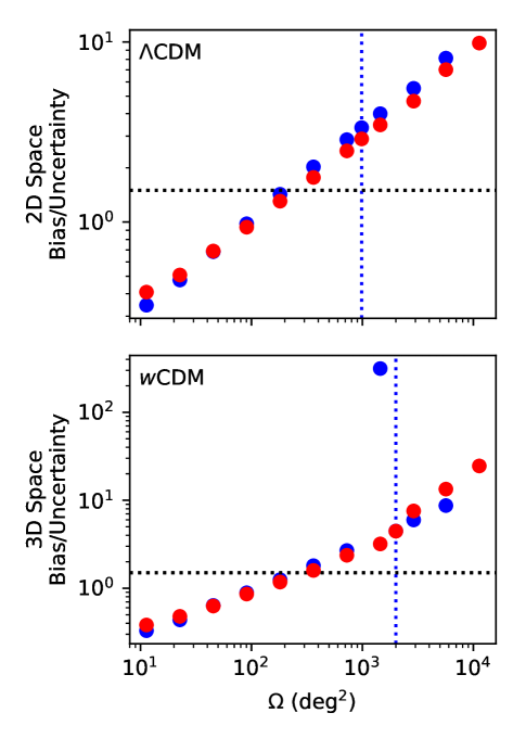
In Figure 13 we illustrate $\mathcal{B}/\mathcal{U}$ as a function of $\Omega$. Results from $n_{\rm pk}$ ($P^{\kappa\kappa}$) are shown using blue (red) markers and lines, and for $\Lambda$CDM ($w$CDM) cosmologies in the top (bottom) panel. The solid vertical lines mark the largest numerically reliable $\Omega$ and the horizontal black dashed lines mark our benchmark for significant error degradation. As in § 3.1.2, we focus on the $\Lambda$CDM case since the $w$ constraints are overall very weak. Figure 13 indicates that at large $\Omega$, $\mathcal{B}/\mathcal{U}$ has a rough power-law dependence on $\Omega$ for both summary statistics. The logarithmic slope of this relation for $n_{\rm pk}$ is $\sim 0.5$, while for $P^{\kappa\kappa}$ it is slightly shallower.

Table 5 summarises the survey sizes $\Omega$ at which the uncertainties in $\hat{\bf p}$ are degraded by $\approx 50\%$. This degradation occurs for both summary statistics and in both $\Lambda$CDM and $w$CDM cosmologies when $\Omega\sim 60~{}{\rm deg}^{2}$. As one might expect, the large, complex photo-$z$ errors studied in this subsection degrade the posteriors considerably more than small residual $b_{\rm ph}$.

Table 5 also includes the unscaled reduced $\chi^{2}$ values of the most likely biased values. Note that these values are not directly comparable to those mentioned in § 3.1.2, since they were not calculated by averaging the sampled $\chi^{2}$ grid computed for each realisation When we construct the unbiased realisation-averaged $\Lambda$CDM posteriors in this way we find that the peak counts and power spectrum have minimum reduced $\chi^{2}$ values of 1.53 and 1.14. We note that this difference in methodology does not alter the location of the unbiased most-likely values and has no noticeable effect on the actual shape of the contours.

Figure 14: Same as Fig. 12 except that the the photometric redshift estimates (in each individual tomographic bin) have been modified by an additive constant, to remove the bias in their centroid in that bin. Consequently, the biases illustrated in this figure arise mostly from differences between the shapes of the redshift distributions $n^{i}_{\rm true}(z)$ and $n^{i}_{\rm ph}(z)$ in each bin $i$.

Figure 15: Same as Fig. 13, except that the biases arise from differences in the shapes of each the redshift distributions $n^{i}_{\rm true}(z)$ and $n^{i}_{\rm ph}(z)$ in each tomographic bin $i$.

Table 6: Summary of cosmological parameter biases arising after the centroid bias of photo-$z$’s in each tomographic bin has been removed. We list the average reduced $\chi^{2}$ values of the most likely values for a single subfield and the survey area $\Omega$ at which parameter estimates are degraded by $\approx 50\%$. For reference, the corresponding average reduced $\chi^{2}$ values of the unbiased best-fit models in a $\Lambda$CDM cosmology from $n_{\rm peaks}$ ($P^{\kappa\kappa}$) are 1.523 (1.14).

model	$n_{\rm peaks}$		$P^{\kappa\kappa}(N_{c}=30)$
	reduced $\chi^{2}$	$\Omega$	reduced $\chi^{2}$	$\Omega$
$\Lambda$CDM	1.21	$200\ {\rm deg}^{2}$	1.09	$248\ {\rm deg}^{2}$
$w$CDM	1.22	$255\ {\rm deg}^{2}$	1.13	$315\ {\rm deg}^{2}$

3.2.2 $n^{i}(z)$ Shape Errors

Finally, we examine the biases in $\hat{\bf p}$ that arise from discrepancies in the shapes of $n^{i}_{\rm true}(z)$ and $n^{i}_{\rm ph}(z)$, assuming perfect removal of centroid bias. As explained above, this approach is equivalent to assuming that a calibration process was able to obtain the correct centroid of the redshift-distribution in each tomographic bin. In practice, we consider each tomographic redshift bin, and shift the $n^{i}_{\rm true}(z)$ by a constant, such that the centroid of the photometric and spectroscopic redshifts coincide. Figures 14 and 15 illustrate the same information as Figures 12 and 13, but they now pertain to errors in the shape of $n^{i}(z)$ (i.e. after the removal of centroid bias). We note that in scaled-up surveys, there is a choice to remove centroid biases either from individual subfields, or from the aggregate of the $N=177$ subfields ($\Omega=2002~{}{\rm deg}^{2}$). In practice we find that this choice makes no discernible difference to the confidence contours.

The left column in Figure 14 shows that the biases in the $95\%$ confidence contours in a single subfield due to shape errors in $n^{i}(z)$ are roughly consistent with being smaller magnitude versions of the shifts that arise from directly approximating $n_{\rm true}(z)$ with $n_{\rm ph}(z)$ (also for a single subfield). However, Figure 14 shows that these trends do not continue for the biases in the highest likelihood regions Instead, we find that the $\Omega_{m}-\sigma_{8}$ contours inferred from $n_{\rm pk}$ shift perpendicular to their direction of degeneracy, toward negative $\Sigma_{8}$, but with some additional shift in the negative $\Omega_{m}$ direction. In contrast, the $\Omega_{m}-\sigma_{8}$ contours from $P^{\kappa\kappa}$ slightly stretch along their direction of degeneracy and shift toward negative $\sigma_{8}$ and positive $\Omega_{m}$. Additionally, we find that the ($\Omega_{m},w$) contours from $n_{\rm pk}$ ($P^{\kappa\kappa}$) slightly shift in the negative (positive) directions of both $\Omega_{m}$ and $w$. While the ($\Omega_{m},w$) contours from $n_{\rm pk}$ expand in the direction of their degeneracy, the $P^{\kappa\kappa}$ contours expand in all directions.

Figure 15 indicates that $\approx 50\%$ degradations occur for $\Lambda$CDM ($w$CDM) constraints inferred from $n_{\rm pk}$ and $P^{\kappa\kappa}$ at survey sizes of 200 (255) deg² and 248 (315) deg². The reduced $\chi^{2}$ values are summarised in Table 6. We remind the reader that the corresponding reduced $\chi^{2}$ values for unbiased cases in $\Lambda$CDM from $n_{\rm pk}$ and $P^{\kappa\kappa}$ are 1.53 and 1.14, respectively.

4 Discussion

We begin this section by first discussing the biases of $\Sigma_{8}$ induced by $b_{\rm ph}$ for the Single-$z$ dataset. A simplistic toy model, assuming that $\kappa$ peaks are entirely explained by lensing from dark matter halos, illustrates why $b_{\rm ph}$ and $\delta\Sigma_{8}$ are anti-correlated. If there is a negative (positive) $b_{\rm ph}$, an observer will mistakenly believe that observed source galaxies are closer to (further from) them than the galaxies are in reality. To produce a given magnitude $\kappa$ value over a shorter (longer) distance, an observer will infer that on average halos must be more (less) massive. This is achieved in cosmologies with larger (smaller) values of $\Sigma_{8}$. The same basic logic applies of course to other over-densities (not just halos), and it also explains the direction of shifts arising from residual $b_{\rm ph}$ in the $\Omega_{m}-\sigma_{8}$ confidence contours in the Tomographic dataset, inferred from either $n_{\rm pk}$ or $P^{\kappa\kappa}$. However, it does not explain the shifts in the most likely values.

A comparison of the shifts in the $\Omega_{m}-\sigma_{8}$ confidence contours from $n_{\rm pk}$ between Figures 5 and 7 illustrates that the combined effects of tomography and $|b_{\rm ph}|\propto z$ induce more complex changes in the posteriors of $\hat{\bf p}$. At the same time, comparisons of the shifts in the contours of Figure 7 inferred by $n_{\rm pk}$ and $P^{\kappa\kappa}$ suggest that $P^{\kappa\kappa}$ is more resilient to $b_{\rm ph}$ than $n_{\rm pk}$.

To assess the validity of $\mathcal{B}/\mathcal{U}$ as our proxy for error degradation, we compare our findings, regarding the impact of $b_{\rm ph}$ on the inference of a $w$CDM cosmology using $P^{\kappa\kappa}$, with those of Huterer et al. (2006). Their analysis employs a Fisher Matrix formalism to model degradations in the marginalised error of $\Omega_{m}$, $\sigma_{8}$, and $w$ induced by residual centroid biases $\delta z$. Huterer et al. (2006) define 10 tomographic bins, of equal widths spanning $0<z_{\rm ph}<3.0$, and model the priors on $\delta z$ as independent zero-mean Gaussians with identical variances $\Delta^{2}$.

The choices of tomographic bins, higher shape noise, and higher total galaxy surface density made by Huterer et al. (2006) cause their 2 (4) tomographic bins at $z>2.4$ ($z<0.3$ and $1.5<z<2.4$) to have values of $(\sigma_{\gamma}^{2}/n^{i}_{g})$ that are factors of $\sim 7-13$ ($\sim 1.3-4$) larger than the corresponding value averaged over all of our tomographic bins. Note that $n^{i}_{g}$ indicates the galaxy number density for tomographic bin $\bar{z}_{b}$. Because the covariance of $P^{\kappa\kappa}(\ell,\bar{z}_{b},\bar{z}_{b}^{\prime})$ and $P^{\kappa\kappa}(\ell,\bar{z}_{b},\bar{z}_{b}^{\prime\prime})$ is correlated with $(\sigma_{\gamma}^{2}/n^{i}_{g})$, these choices lead Huterer et al. (2006) to infer slightly weaker undegraded constraints and sensitivity of $P^{\kappa\kappa}$ to $\delta z$. Our use of each galaxy’s photo-$z$ point estimate for ray-tracing (rather than drawing from redshifts $\hat{n}^{i}(z)$) also augments this effect. At the same time, both their use of an LSST-like $n_{\rm true}(z)$ peaking at $z=0.7$ (rather than 0.6) and their calculation of $P^{\kappa\kappa}$ over a $\sim 60\%$ larger multipole range ($50<\ell<3000$) has the opposite effect.

For 4900 and 6300 square degree surveys, Huterer et al. (2006) finds $50\%$ marginalised error degradations when the priors on $\delta z$ have $\Delta$ $\sim 0.0019-0.0026$ and $\sim 0.0017-0.0023$. For simple comparison to our results, we assume that the error degradations occur when $|\delta z|\sim\Delta$. At the same survey sizes, we find $\approx 50\%$ degradation in the posterior when $b$ is $-0.003$ and $0.003$, respectively. In our analysis, $|b|=0.003$ corresponds to $|\delta z|\sim 0.0037-0.0089$, with larger magnitudes at larger $\bar{z}_{b}$. At the $\bar{z}_{b}$ where the results of Huterer et al. (2006) are most relevant ($z\sim 0.5-1$), we predict $50\%$ degradations for effective centroid biases, $|\delta z|\sim 0.0046-0.0060$. These values are reassuringly close Huterer et al. (2006)’s; i.e. factors of $\sim 1.8-3.5$ larger than their results.

We next turn our attention to Figure 10, which shows the maximum survey size at which error degradation from $b_{\rm ph}$ is tolerable, as a function of $b$. For the most pessimistic cases of $b_{\rm ph}$ that satisfy the LSST photo-$z$ requirements ($|b|=0.003$), we find $\sim 50\%$ error degradations can occur in the inferred posteriors of a $\Lambda$CDM cosmology using $n_{\rm pk}$ ($P^{\kappa\kappa}$) in surveys as small as $\Omega\sim 1300\ {\rm deg}^{2}$ ($\sim 6500\ {\rm deg}^{2}$). Figure 10 also reinforces the idea that $P^{\kappa\kappa}$ is less sensitive than $n_{\rm pk}$ to $b_{\rm ph}$, independent of our model cosmology type.

We next compare our results for uncalibrated photo-$z$ errors with those of P16. Their analysis quantified the joint impact of both $b_{\rm ph}=0.003(1+z)$ and scatter in $z_{\rm ph}$ on $\hat{\bf p}$ using the power spectrum and scaled peak counts with 5 tomographic bins. Their assessment assumed linear dependence of the (mean) summary statistic ${\bf d}({\bf p})$ on cosmology ${\bf p}$. Additionally, they held $\hat{n}(z)$ across tomographic bins equal to $n_{\rm true}(z)$ and only allowed photo-$z$ errors to reshuffle redshifts between tomographic bins (modifying $\hat{n}^{i}(z)$). Keeping these difference in mind, we compare the shifts in the ($\Omega_{m},w$) contours of Figure 8 arising from $b=0.003$ with the distribution of biased most likely ($\Omega_{m},w$) values reported by P16 inferred from 20 semi-independent mock observations of an LSST-sized survey area. Although our results basically agree on the directions of the biases, P16 finds that $P^{\kappa\kappa}$ is more sensitive to $b_{\rm ph}$ than $n_{\rm pk}$ and that unbiased cosmology is included within the $68\%$ confidence contour of the distribution of the biased values inferred with $n_{\rm pk}$.

Though many of the differences in our analyses may contribute to this discrepancy, one compelling explanation is our choice of tomographic bins. P16 attributes their finding of extra resilience of $n_{\rm pk}$ to photo-$z$ errors to the absence of spatial correlation in photo-$z$ errors coupled with the fact that peak locations are determined by the shapes of several neighboring source galaxies. Our choice of tomographic bins reduces our average surface density of galaxies per bin ($\sim 0.4$ galaxies per pixel) to half that of P16. Because we have fewer galaxies around each peak, our $n_{\rm pk}$ may be more sensitive to photo-$z$ errors. The sensitivity of $P^{\kappa\kappa}$ to $b_{\rm ph}$ probably has weaker dependence on our choice of bins because we compute cross-spectra for each combination of bins. If we were to repeat our analysis only using 5 tomographic bins, we expect $n_{\rm pk}$ to be have resilience to photo-$z$ errors better than or comparable to that of $P^{\kappa\kappa}$. We defer exploration of this to future work.

The shifts of the $95\%$ contours in Figure 12 suggests that the lower sensitivity of $P^{\kappa\kappa}$ to $b_{\rm ph}$ does not extend to arbitrary photo-$z$ errors. Joint examination of the biases induced by different classes of photo-$z$ errors, in Figure 8 and in the right columns of Figures 12 and 14, hints at the utility of employing $n_{\rm pk}$ alongside $P^{\kappa\kappa}$ for large surveys ($\Omega\ga 2002~{}{\rm deg}^{2}$). Figure 8 shows that the $\Omega_{m}-w$ contours inferred from the two statistics have slightly different dependences on $b_{\rm ph}$ while the other figures show that the biases on $\hat{\bf p}$ are very different for each statistic for more complex photo-$z$ errors. This suggests that the using $n_{\rm pk}$ alongside $P^{\kappa\kappa}$ might allow for self-calibration of photo-$z$ errors.

We next turn to the main results of § 3.2.1: for surveys as small as $\Omega\sim 60\ {\rm deg}^{2}$, with LSST-like $n_{\rm ph}(z)$ and photo-$z$ error, the approximation of $n_{\rm true}(z)$ with $n_{\rm ph}(z)$ degrades the posterior of $\hat{\bf p}$ by $\sim 50\%$. This implies a very strong bias, as the existing surveys already cover areas that exceed $60\ {\rm deg}^{2}$. However, our result has no direct implication for current surveys with comparable or better sensitivity, such as DES Y1 (Troxel et al., 2017), because these surveys already employ better estimates of $n_{\rm true}(z)$. E.g. the estimation of $n_{\rm true}(z)$ by stacking the individual redshift posteriors for each galaxy (rather than using the photo-$z$ point estimates) and by trying to remove centroid biases. To remove the centroid bias, these surveys use calibration techniques to place relatively tight priors on these biases which they then use when simultaneously inferring the cosmological parameters, the sizes of the centroid biases, and other nuisance parameters.

In § 3.2.2, we assess the impact of errors in the shape of $n^{i}(z)$ assuming that centroid biases have been perfectly removed during the estimation of $n^{i}_{\rm true}(z)$ with $n^{i}_{\rm ph}(z)$. This is analogous to how current surveys remove centroid biases from their $\hat{n}^{i}(z)$. We find $\approx 50\%$ error degradations to $\Lambda$CDM ($w$CDM) constraints using $n_{\rm pk}$ and $P^{\kappa\kappa}$ for surveys with $\Omega=200$ (250) ${\rm deg}^{2}$ and $\Omega=248$ (315) ${\rm deg}^{2}$. These results still do not apply directly to current surveys, as our unbiased case at 200 square degrees provides tighter constraints than DES Y1 (Troxel et al., 2017) and the first year of HSC (Hikage et al., 2018), the current surveys with the strongest constraints. The tighter undegraded constraints make our relative biases larger. Moreover, the fact that our $\hat{n}^{i}(z)$ is based on the distribution of photo-$z$ point-estimates means that the errors in our final $\hat{n}^{i}(z)$ are larger than those of either survey.

As explained in the beginning of § 3.2, the results of § 3.2.1 are  3.2.2 are each pessimistic. In reality, a survey with an LSST-like photo-$z$ distribution and galaxy distribution would not encounter considerable degradations until survey sizes somewhat larger than we quote.

Finally, we emphasise that this work made a number of simplifying assumptions. Throughout our analysis involving the Tomographic dataset, we assumed that $\mathcal{B}/\mathcal{U}$ is a good proxy for error degradation, rather than propagating the uncertainties in the inferred $\hat{n}(z)$ distributions allowed by the photo-$z$ errors. We also assumed that using the predicted LSST spectroscopic galaxy distribution as the estimate for the photo-$z$ distribution would incur negligible errors. In § 3.2.1, we did not attempt to infer the MLE of $n_{\rm true}(z)$. Additionally, we assumed that the $p(e_{z}|z_{\rm ph})$ of the simulated survey and calibration set were equivalent and that $p(e_{z}|z_{\rm ph})$ is well described by a histogram. Future work needs to improve on our results by addressing these assumptions. Furthermore, it is worth assessing how the inclusion of Euclid photometry improves our survey limits; Rhodes et al. (2017) showed using Euclid can improve the scatter and outlier fraction of the photo-$z$ PDF by a factor of 2 for $1.5<z<3$ and improved the scatter by $\sim 30\%$ at other $z$.

5 Conclusions

Photo-$z$ errors are expected to be one of the leading systematic errors in future WL surveys. In this paper, we have assessed the impact of two classes of photo-$z$ errors on cosmological parameters inferred from tomographic peak counts and the tomographic power spectrum. Other sources of systematics not addressed in this work include intrinsic alignment, measurement errors (correlated PSF residuals; de-blending; shape measurements), and other theoretical errors (simulation accuracy, finite number of realisations, baryonic effects).

To assess the implications of these errors, we use ray-tracing simulations with a simple approach of modelling photo-$z$ errors to produce mock shape catalogues in $\sim 10$ deg² subfields of an LSST-like survey. We focus primarily on quantifying the degradation of constraints for a $\Lambda$CDM cosmology (but also consider a $w$CDM cosmology). We address the degradations from residual photo-$z$ biases and from a (mis)estimation of the true galaxy distribution $n_{\rm true}(z)$ with various $n_{\rm ph}(z)$, distributions of photo-$z$ point estimates, using LSST-like photometric measurements.

Our main findings can be enumerated as follows.

1. The power spectrum is more resilient than peak counts to residual photo-$z$ biases. However, both summary statistics appear to be similarly sensitive to more complex alterations to the inferred galaxy redshift distribution.

2. Pessimistic cases of residual photo-$z$ biases that satisfy the LSST photo-$z$ requirements can significantly degrade constraints. They can degrade constraints from surveys with an LSST-like galaxy redshift distribution, utilising lensing peak counts (the convergence power spectrum), as small as $\Omega\sim 1200\ {\rm deg}^{2}$ ($\sim 6300\ {\rm deg}^{2}$) by $\approx 50\%$.

3. Generally, surveys with LSST-like galaxy redshift distributions and LSST-like photo-$z$ only as small as $\Omega\sim 60\ {\rm deg}^{2}$ can directly approximate $n_{\rm true}(z)$ with $n_{\rm ph}(z)$ without degrading their constraints by $\ga 50\%$.

4. If such surveys successfully remove the biases in the centroid of the photo-$z$ distribution in each tomographic bin, these critical survey sizes, corresponding to $\approx 50\%$ parameter degradation, increase to $\Omega\sim 200\ {\rm deg}^{2}$ for lensing peaks, and to $\sim 250\ {\rm deg}^{2}$ for the power spectrum.

5. The last result implies that even without centroid biases, the width and large tails of the unoptimised predicted photo-$z$ PDF can significantly bias parameters. This needs to be further mitigated with more sophisticated approaches of estimating $n_{\rm true}(z)$ (such as stacking redshift posteriors).

Future work is needed to more fully understand the impact of photo-$z$ errors on non-Gaussian summary statistics in an LSST-like survey. Such work should include the simultaneous inference of cosmological parameters and the underlying galaxy redshift distribution in order to propagate uncertainties in the true underlying galaxy distribution to the final constraints. It should also employ realistic photo-$z$ errors and include the impact of uncalibrated photo-$z$ errors. Other related necessary work includes assessing the impact of photo-$z$ errors on the inference of more complex dark energy equations of state with non-Gaussian statistics and assessing the efficacy of employing multiple summary statistics for self-calibration of photo-$z$ errors.

Appendix A Boundary Conditions

In this appendix we briefly discuss the impact of the boundary conditions during the Kaiser-Squire Transform and Gaussian smoothing. Per the discrete convolution theorem (Press et al., 1992), the straight-forward application of the Kaiser-Squire Transform effectively assumes a periodic boundary condition. Lanusse et al. (2016) points out that the equivalent real-space convolution kernel falls off as the angular transverse distance squared and by zero padding the shear map, we can mitigate the effects of the periodic boundary condition. Upon comparing the peak count histograms (see the end of this section) with and without zero-padding (the Fourier transforms were performed on an array with 4 times as many pixels in the zero-padded case), we conclude that the error introduced by assuming a periodic boundary condition is negligible.

For the Gaussian smoothing, we compare the variability in the relative differences between outlying $\kappa$ values arising from different choices of boundary condition and the global variability of $\kappa$ in a smoothed map. To measure variability, we use the median absolution deviation ($MAD$). The relative differences are computed for a periodic boundary condition with respect to a boundary condition in which the values are mirrored across the center of the last pixel (the first repeated value is the second pixel from the edge). We find that $MAD$s are comparable when considering a square annulus of $\kappa$ values 8 pixels away from the edge.

Appendix B Simulated Realistic photo-$z$ Performance

Figure 16: Performance of realistic photo-$z$’s as a function of spectroscopic $z$ for bins with a width $\Delta z=0.05$. For each $z$ bin, we show the bias $b_{\rm ph}/(1+z)$, which is the median of $e_{z}=(z_{\rm ph}-z)/(1+z)$ (top), the scatter $\sigma_{F}$ about $b_{\rm ph}/(1+z)$ (middle), and the catastrophic outlier rate, defined here as the percentage of galaxies more than $3\sigma_{F}$ from bin. Specifically, the blue (red) lines indicate measurements when we define $\sigma_{F}$ as the interquartile range of $e_{z}$ divided by 1.38 (median absolute deviation of $e_{z}$ times 1.48). In each panel, the gray lines indicate the LSST photo-$z$ requirements (LSST Science Collaboration et al., 2009). Due to the large magnitudes of $b_{\rm ph}/(1+z)$, the gray dashed lines shown indicate the joint weak lensing and galaxy clustering analysis requirement, $|b_{\rm ph}|<0.01(1+z)$, rather than the more strict requirement for weak lensing alone. The dashed lines in the middle panel indicate the strict requirement that $\sigma_{z}/(1+z)$ is less than 0.05 and illustrate the target value of 0.02.

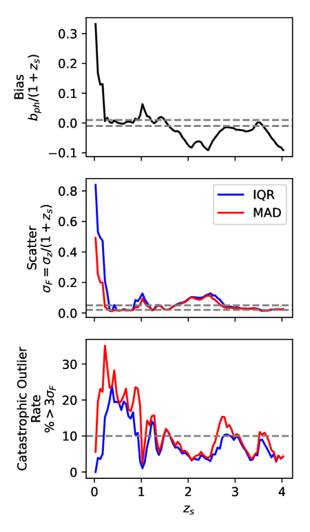
In this appendix, we quantify the performance of the simulated LSST-like photo-$z$ measurements discussed in § 2.4.2. Figure 16 shows the bias, scatter, and catastrophic error rate as a function of the true spectroscopic rate. The figure clearly shows that for each of these metrics, the realistic photo-$z$ measurements do not meet the LSST photo-$z$ requirements outlined in LSST Science Collaboration et al. (2009).

Additionally, we compare our simulated photo-$z$ performance to that of the DES Y1 analysis, which currently provides one of the tightest sets of weak lensing (Troxel et al., 2017). To do this, we measure metrics of the distributions of $R$, the difference between the photo-$z$ point estimate and its true spectroscopic redshift, for each tomographic bin. Specifically, we measure $\sigma_{68}(R)$, which is the half-width of the span of $68\%$ of values spanning the median of $R$, and the outlier fraction, which measures the fraction of $R$ values that deviate by more than $2\times\sigma_{68}(R)$ from the median of $R$. In Table 7 we list each of these metrics computed for a single subfield averaged over the 1000 realisations of $\hat{{\boldsymbol{\gamma}}}_{\rm obs}({\boldsymbol{\theta}}_{g},z_{g})$ used to asses the impact of unmodelled photo-$z$ error.

The measurements listed in Table 7 are directly comparable to those listed in Table 3 of Hoyle et al. (2018) for the BPZ ${\sc metacalibration}$, the same photo-$z$ distribution used to infer DES Y1 cosmology constraints (Troxel et al., 2017). Our 8 lowest redshift bins each have a smaller $\sigma_{68}(R)$ than any of the bins employed for DES Y1, which are each about $\sim$0.14. However, all of our bins have outlier percentages that are larger by a factor of $\sim$2$-$6. We note that our definition of $R$ slightly deviates from that of Hoyle et al. (2018) due to our knowledge of the true spectroscopic redshift of each galaxy in our mock survey. We also note that the DES Y1 analysis only used these point estimates for identifying each galaxy’s tomographic bin. The $\hat{n}^{i}(z)$ they use for cosmological inference was actually constructed by stacking the full the redshift posteriors produced for each galaxy by their photo-$z$ method (Hoyle et al., 2018). Consequently, their estimates of $n^{i}_{\rm true}(z)$ are likely better than ours.

Table 7: Performance metrics for the simulated realistic photo-$z$ bin measurements from (Rhodes et al., 2017), averaged over 1000 realisations. Each metric is computed for the distribution of residuals $R=z_{\rm ph}-z$ in a given tomographic bin. We include $\sigma_{68}(R)$, which is half of the span of $68\%$ of the $R$ values centered on the median of $R$, and Outlier Percentage, which is the percentage of values more than $2\sigma_{68}(R)$ from the median residual.

$z_{\rm ph}$ range	$\sigma_{68}(R)$	Outlier Percentage
$[0,0.332)$	$0.02171\pm 0.00017$	$20.11\pm 0.09$
$[0.332,0.464)$	$0.0348\pm 0.0003$	$22.36\pm 0.08$
$[0.464,0.577)$	$0.0438\pm 0.0004$	$18.90\pm 0.09$
$[0.577,0.689)$	$0.0359\pm 0.0004$	$19.33\pm 0.08$
$[0.689,0.806)$	$0.0409\pm 0.0003$	$16.63\pm 0.08$
$[0.806,0.936)$	$0.0616\pm 0.0005$	$17.24\pm 0.08$
$[0.936,1.089)$	$0.1031\pm 0.0007$	$18.65\pm 0.08$
$[1.089,1.287)$	$0.1395\pm 0.0007$	$17.67\pm 0.09$
$[1.287,1.596)$	$0.2772\pm 0.0014$	$12.82\pm 0.11$
$[1.596,3]$	$0.310\pm 0.003$	$14.91\pm 0.13$

Appendix C Interpolation Comparison

Figure 17: Accuracy of different methods for interpolating summary statistics between cosmologies. Each panel shows the distribution of the $95\%$ lowest magnitude differences between predicted and true values relative to the standard deviation of each component of a summary statistic, with $\sigma\neq 0$, for all 100 sampled cosmologies of the Shape Catalog Dataset. The summary statistic used to generate this figure is $n_{\rm pk}$ with 30 $\nu$ bins per tomographic peak. Every panel other than the lower right shows the performance of RBF interpolation (blue) and augmented RBF interpolation (green) using the unaltered components of $n_{\rm pk}$ with a different a basis function. In those panels we also show the performance of RBF interpolation for the components of $n_{\rm pk}$ subtracted by their cosmology averaged values (orange). The lower right panel shows the performance of Gaussian Process interpolation. Specifically, the panel shows the histograms for unaltered components using interpolation that accounts (does not account) for the variance in black (red) and for components rescaled such that the collection of a given component for all sampled cosmologies has unit standard deviation.

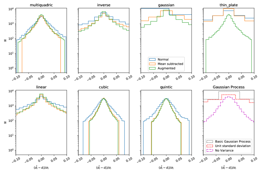
Here we describe the accuracies of different schemes to interpolate a summary statistic ${\bf d}$ as a function of cosmology. The emulator interpolates $d_{k}$, the $k^{\rm th}$ component of a summary statistic, at an arbitrary cosmology using the expectation values $\{d_{k,1},d_{k,2},...,d_{k,P}\}$ in $P$ nearby sampled cosmologies $\{{\bf p}_{1},{\bf p}_{2},...{\bf p}_{P}\}$. The interpolation of each component is performed independently.

By default, the emulator framework provided by LensTools use Radial Basis Function (RBF) interpolation. For some basis function basis function $\phi(r)$, where $r=\sqrt{{\bf p}^{2}-{\bf p^{\prime}}^{2}}$ is the distance between two cosmologies in parameter space, the emulator predicts the $k$th component as

$$\hat{d}_{k}({\bf p})=\sum_{i}^{P}\lambda_{i}\phi(\sqrt{{\bf p}^{2}-{\bf p}_{i}^{2}}).$$ (14)

The values of $\{\lambda_{1},\lambda_{2},...,\lambda_{P}\}$ are the solutions to the system of equations obtained by plugging $\{{\bf p}_{1},{\bf p}_{2},...{\bf p}_{P}\}$ and $\{d_{k,1},d_{k,2},...,d_{k,P}\}$ into Equation 14.

Liu et al. (2015a) found that using a “multi-quadric” basis function, $\phi(r)=\sqrt{(r/\epsilon)^{2}+1}$ ($\epsilon$ is a constant typically set to the average distance between every pair of sampled cosmologies) gave the most accurate results. However, our use of PCA to reduce dimensionality complicates our choice of interpolation method. The whitening step of PCA involves the subtraction of a constant value $C$, the average value of $\{d_{k,1},d_{k,2},...,d_{k,P}\}$, from the $d_{k}$ of every sampled cosmology. We define $d_{k,\ell}^{\prime}=(d_{k,\ell}-C)$. Assuming that $d_{k}$ is not constant for every sampled cosmology and that $C$ is non-zero, $(d_{k,\ell}-C)/d_{k,\ell}$ is not constant for all $\ell$. Consequently, RBF interpolation can predict different values for $d_{k,\ell}^{\prime}+C$ and $d_{k,\ell}$ at a cosmology that was not sampled. To help address this issue, we introduce another interpolation technique called augmented RBF interpolation (Wright, 2003). This method involves simultaneously performing RBF and linear interpolations. The addition of a constant by the linear interpolation makes this technique’s predictions invariant to constant offsets of $d_{k}$.

At this point we turn our attention to comparing the relative accuracy of different interpolation methods. To do this, we select a cosmology ${\bf p}_{j}$ of the Tomographic dataset from the $\{{\bf p_{i}}\}$ and predict $\hat{d}_{k}$ in this cosmology with an emulator constructed from $\{{\bf p_{i}}\}$ but excluding ${\bf p}_{j}$. For this exercise, we choose to use the tomographic peak count histogram, constructed with 30 equally sized $\nu$ bins in each tomographic bin spanning the ranges given in Table 2. We then compute $(\hat{d}_{k}-d_{k})/\sigma_{k}$ where $\sigma_{k}^{2}$ is the variance of $d_{k}$, computed from all $N_{r}=16000$ realisations of $\hat{\kappa}_{r}({\boldsymbol{\theta}}_{p},\bar{z}_{b};{\bf p}_{j})$. We repeat this process for all $N_{b}=300$ components of ${\bf d}$ and each ${\bf p}_{j}$ in $\{{\bf p_{i}}\}$.

Figure 17 shows histograms of the $95\%$ lowest magnitude values of all $(\hat{d}_{k}-d_{k})/\sigma_{k}$ with non-zero $\sigma_{k}$ for different interpolation methods. Each panel, other than the bottom right, shows histograms for a given radial basis function, offered by scipy (Jones et al., 2001). In these panels, the green (blue/orange) line indicates the histogram using augmented RBF interpolation (normal RBF interpolation on $d_{k}$ / on $d_{k}-C$). The bottom right corner shows the performance for a naive application of the Gaussian Process interpolation implemented by scikit-learn (Pedregosa et al., 2011), with and without including the $\sigma_{k}^{2}$ in the interpolation. It also shows the performance of Gaussian Process interpolation applied such that the collection of values of a given component of the summary statistic for all sampled cosmologies has a standard deviation of 1.

Based on these results, we chose to use augmented RBF interpolation with cubic basis functions ($r^{3}$), which gives the second-best results in Figure 17. While quintic basis functions ($r^{5}$) yields marginally more accurate results (i.e. a somewhat narrower distribution than the cubic case), we chose cubic basis functions because they are simpler and the difference is barely perceptible. Future work on this topic should assess the impact of the relative scaling of different cosmological parameters in distance calculations and assess the performance of more carefully tuned Gaussian Process interpolation.

Appendix D PCA Application

Figure 18: The top row illustrates the marginalised posteriors for $\Omega_{m}$ (left), $w$ (center), $\sigma_{8}$ (right) achieved with different numbers of principal components ($N_{c}$) of the peak count histogram. Panels in the bottom row show the evolution of the standard deviations of the relevant marginalised posteriors as a function of $N_{c}$. The dotted black line shows the standard deviation of the full peak count histogram without any PCA. The data illustrated in this plot has been scaled up to a survey with $N=123$ fields.

Figure 19: Same as Figure 18 except for the power spectrum.

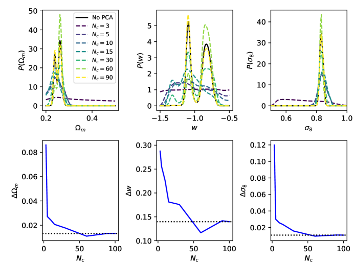
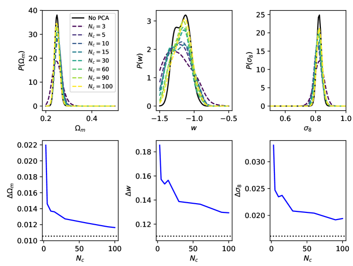
In this appendix we describe the process to identify the number of principal components, $N_{c}$ used to represent each summary statistic. To do this, we examined the change in the marginalised standard deviations of each of the parameters in $w$CDM for a survey scaled up to $N=123$ subfields (the maximum size allowed for the full power spectrum). The top row of Figure 18 (Figure 19) illustrates the marginalised posteriors for different numbers of principal components of the tomographic peak count histograms (tomographic power spectrum) while the bottom row illustrates the change in the marginalised standard deviation as functions of $N_{c}$. We found negligible difference in employing the standard deviation from using the size of the $68\%$ confidence interval.

Because of the dip in the marginalised standard deviations for the peak counts when using $N_{c}=60$ below the marginalised standard deviations using the entire feature set we elect to use the full peak count histogram histogram in our analysis to avoid misleading results. (This is equivalent to using $N_{c}=100$). Since the rate at which the marginalised standard deviation decreases, largely levels off at $N_{c}=30$, we elect to use $N_{c}=30$ principal components for the power spectrum.

Appendix E Larger Residual Bias

Figure 20: Same as Figure 7, except that the residual biases have much larger magnitudes.

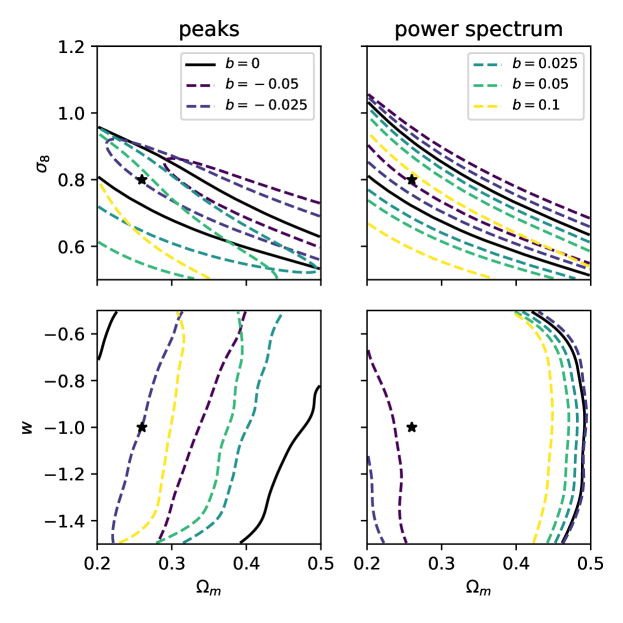
This appendix includes Figure 20 which illustrates the $95\%$ confidence contours which arise from larger residual biases than considered in the main text. These residual biases are also considerably larger than those allowed by the LSST science requirements and are shown here for completeness.

References

- Abbott et al. (2016) Abbott T., et al., 2016, Phys. Rev. D, 94, 022001
- Abdalla et al. (2008) Abdalla F. B., Amara A., Capak P., Cypriano E. S., Lahav O., Rhodes J., 2008, MNRAS, 387, 969
- Aihara et al. (2018) Aihara H., et al., 2018, PASJ, 70, S4
- Albrecht et al. (2006) Albrecht A., et al., 2006, ArXiv Astrophysics e-prints,
- Bernstein & Huterer (2010) Bernstein G., Huterer D., 2010, MNRAS, 401, 1399
- Bridle & King (2007) Bridle S., King L., 2007, New Journal of Physics, 9, 444
- Cunha et al. (2012) Cunha C. E., Huterer D., Busha M. T., Wechsler R. H., 2012, MNRAS, 423, 909
- Cunha et al. (2014) Cunha C. E., Huterer D., Lin H., Busha M. T., Wechsler R. H., 2014, MNRAS, 444, 129
- DES Collaboration (2005) DES Collaboration 2005, ArXiv Astrophysics e-prints,
- DES Collaboration et al. (2017) DES Collaboration et al., 2017, preprint, (arXiv:1708.01530)
- Freedman & Diaconis (1981) Freedman D., Diaconis P., 1981, Zeitschrift für Wahrscheinlichkeitstheorie und Verwandte Gebiete, 57, 453
- Fu et al. (2014) Fu L., et al., 2014, MNRAS, 441, 2725
- Gupta et al. (2018) Gupta A., Matilla J. M. Z., Hsu D., Haiman Z., 2018, Phys. Rev. D, 97, 103515
- Hartlap et al. (2007) Hartlap J., Simon P., Schneider P., 2007, A&A, 464, 399
- Hearin et al. (2010) Hearin A. P., Zentner A. R., Ma Z., Huterer D., 2010, ApJ, 720, 1351
- Hearin et al. (2012) Hearin A. P., Zentner A. R., Ma Z., 2012, J. Cosmology Astropart. Phys., 4, 034
- Hikage et al. (2018) Hikage C., et al., 2018, preprint, (arXiv:1809.09148)
- Hilbert et al. (2009) Hilbert S., Hartlap J., White S. D. M., Schneider P., 2009, A&A, 499, 31
- Hildebrandt et al. (2017) Hildebrandt H., et al., 2017, MNRAS, 465, 1454
- Hinshaw et al. (2013) Hinshaw G., et al., 2013, ApJS, 208, 19
- Hoyle et al. (2018) Hoyle B., et al., 2018, MNRAS, 478, 592
- Hunter (2007) Hunter J. D., 2007, Computing in Science & Engineering, 9, 90
- Huterer et al. (2006) Huterer D., Takada M., Bernstein G., Jain B., 2006, MNRAS, 366, 101
- Ivezić et al. (2008) Ivezić Ž., et al., 2008, preprint, (arXiv:0805.2366)
- Ivezić et al. (2014) Ivezić Ž., Connolly A. J., VanderPlas J. T., Gray A., 2014, Statistics, Data Mining, and Machine Learning in Astronomy. Princeton University Press
- Jain et al. (2000) Jain B., Seljak U., White S., 2000, ApJ, 530, 547
- Jain et al. (2007) Jain B., Connolly A., Takada M., 2007, J. Cosmology Astropart. Phys., 3, 013
- Jones et al. (2001) Jones E., Oliphant P., Peterson P., et al., 2001, SciPy: Open source scientific tools for Python, http://www.scipy.org/
- Kacprzak et al. (2016) Kacprzak T., et al., 2016, MNRAS, 463, 3653
- Kaiser & Squires (1993) Kaiser N., Squires G., 1993, ApJ, 404, 441
- Kilbinger et al. (2013) Kilbinger M., et al., 2013, MNRAS, 430, 2200
- Kitching et al. (2008) Kitching T. D., Taylor A. N., Heavens A. F., 2008, MNRAS, 389, 173
- LSST Science Collaboration et al. (2009) LSST Science Collaboration et al., 2009, preprint, (arXiv:0912.0201)
- Laigle et al. (2016) Laigle C., et al., 2016, ApJS, 224, 24
- Lanusse et al. (2016) Lanusse F., Starck J.-L., Leonard A., Pires S., 2016, A&A, 591, A2
- Laureijs et al. (2011) Laureijs R., et al., 2011, preprint, (arXiv:1110.3193)
- Leistedt et al. (2016) Leistedt B., Mortlock D. J., Peiris H. V., 2016, MNRAS, 460, 4258
- Lin & Kilbinger (2015) Lin C.-A., Kilbinger M., 2015, A&A, 576, A24
- Liu et al. (2014) Liu J., Haiman Z., Hui L., Kratochvil J. M., May M., 2014, Phys. Rev. D, 89, 023515
- Liu et al. (2015a) Liu J., Petri A., Haiman Z., Hui L., Kratochvil J. M., May M., 2015a, Phys. Rev. D, 91, 063507
- Liu et al. (2015b) Liu X., et al., 2015b, MNRAS, 450, 2888
- Ma & Bernstein (2008) Ma Z., Bernstein G., 2008, ApJ, 682, 39
- Ma et al. (2006) Ma Z., Hu W., Huterer D., 2006, ApJ, 636, 21
- Martinet et al. (2018) Martinet N., et al., 2018, MNRAS, 474, 712
- McKinney (2010) McKinney W., 2010, in van der Walt S., Millman J., eds, Proceedings of the 9th Python in Science Conference. pp 51–56
- Pedregosa et al. (2011) Pedregosa F., et al., 2011, Journal of Machine Learning Research, 12, 2825
- Petri (2016) Petri A., 2016, Astronomy and Computing, 17, 73
- Petri et al. (2014) Petri A., May M., Haiman Z., Kratochvil J. M., 2014, Phys. Rev. D, 90, 123015
- Petri et al. (2015) Petri A., Liu J., Haiman Z., May M., Hui L., Kratochvil J. M., 2015, Phys. Rev. D, 91, 103511
- Petri et al. (2016) Petri A., May M., Haiman Z., 2016, Phys. Rev. D, 94, 063534
- Press et al. (1992) Press W. H., Teukolsky S. A., Vetterling W. T., Flannery B. P., 1992, Numerical Recipes in C (2Nd Ed.): The Art of Scientific Computing. Cambridge University Press, New York, NY, USA
- Rau et al. (2017) Rau M. M., Hoyle B., Paech K., Seitz S., 2017, MNRAS, 466, 2927
- Rhodes et al. (2017) Rhodes J., et al., 2017, ApJS, 233, 21
- Ribli et al. (2018) Ribli D., Ármin Pataki B., Csabai I., 2018, preprint, (arXiv:1806.05995)
- Robitaille et al. (2013) Robitaille T. P., et al., 2013, A&A, 558, A33
- Schmelzle et al. (2017) Schmelzle J., Lucchi A., Kacprzak T., Amara A., Sgier R., Réfrégier A., Hofmann T., 2017, preprint, (arXiv:1707.05167)
- Schneider (2005) Schneider P., 2005, ArXiv Astrophysics e-prints,
- Shirasaki & Yoshida (2014) Shirasaki M., Yoshida N., 2014, ApJ, 786, 43
- Shirasaki et al. (2013) Shirasaki M., Yoshida N., Hamana T., 2013, ApJ, 774, 111
- Song & Knox (2004) Song Y.-S., Knox L., 2004, Phys. Rev. D, 70, 063510
- Spergel et al. (2015) Spergel D., et al., 2015, preprint, (arXiv:1503.03757)
- Springel (2005) Springel V., 2005, MNRAS, 364, 1105
- Troxel et al. (2017) Troxel M. A., et al., 2017, preprint, (arXiv:1708.01538)
- Wilson & Fonner (2014) Wilson L. A., Fonner J. M., 2014, in Proceedings of the 2014 Annual Conference on Extreme Science and Engineering Discovery Environment. XSEDE ’14. ACM, New York, NY, USA, pp 40:1–40:8, doi:10.1145/2616498.2616534, http://doi.acm.org/10.1145/2616498.2616534
- Wright (2003) Wright G. B., 2003, Phd thesis, University of Colorado, Boulder, http://math.boisestate.edu/~wright/research/GradyWrightThesis.pdf
- Yang et al. (2011) Yang X., Kratochvil J. M., Wang S., Lim E. A., Haiman Z., May M., 2011, Phys. Rev. D, 84, 043529
- Zorrilla Matilla et al. (2016) Zorrilla Matilla J. M., Haiman Z., Hsu D., Gupta A., Petri A., 2016, Phys. Rev. D, 94, 083506
- Zorrilla Matilla et al. (2017) Zorrilla Matilla J. M., Haiman Z., Petri A., Namikawa T., 2017, Phys. Rev. D, 96, 023513
- de Jong et al. (2013) de Jong J. T. A., Verdoes Kleijn G. A., Kuijken K. H., Valentijn E. A., 2013, Experimental Astronomy, 35, 25
- de Putter et al. (2014) de Putter R., Doré O., Das S., 2014, ApJ, 780, 185
- van Waerbeke (2000) van Waerbeke L., 2000, MNRAS, 313, 524
- van der Walt et al. (2011) van der Walt S., Colbert S. C., Varoquaux G., 2011, Computing in Science & Engineering, 13, 22