Kalman Gradient Descent: Adaptive Variance Reduction in Stochastic Optimization

James Vuckovic (james@jamesvuckovic.com)
Abstract

We introduce Kalman Gradient Descent, a stochastic optimization algorithm that uses Kalman filtering to adaptively reduce gradient variance in stochastic gradient descent by filtering the gradient estimates. We present both a theoretical analysis of convergence in a non-convex setting and experimental results which demonstrate improved performance on a variety of machine learning areas including neural networks and black box variational inference. We also present a distributed version of our algorithm that enables large-dimensional optimization, and we extend our algorithm to SGD with momentum and RMSProp.

1 Introduction

Stochastic optimization is an essential component of most state-of-the-art the machine learning techniques. Sources of stochasticity in machine learning optimization include handling large datasets, approximating expectations, and modelling uncertain dynamic environments. The seminal work of Robbins \BBA Monro (\APACyear1985) showed that, under certain conditions, it is possible to use gradient-based optimization in the presence of randomness. However, it is well-known that gradient randomness has an adverse effect on the performance of stochastic gradient descent (SGD) Wang \BOthers. (\APACyear2013). As a result, the construction of methods to reduce gradient noise is an active field of research Wang \BOthers. (\APACyear2013); Mandt \BBA Blei (\APACyear2014); Grathwohl \BOthers. (\APACyear2017); Roeder \BOthers. (\APACyear2017).

Below, we propose a method using the celebrated Kalman filter Kalman (\APACyear1960) to reduce gradient variance in stochastic optimization in a way that is independent of the application area. Moreover, our method can be combined with existing (possibly application-specific) gradient variance-reduction methods. The specific contributions of this paper are:

  • A novel framework for performing linear filtering of stochastic gradient estimates in SGD;

  • Analysis of the asymptotic properties of the filter and a proof of convergence for the resulting optimization algorithm;

  • Extensions of the proposed framework to modern optimization algorithms, and analysis of asymptotic filter properties in these cases;

  • A novel, distributed variant of these algorithms to deal with high-dimensional optimization;

  • Experiments comparing our algorithm to traditional methods across different areas of machine learning, demonstrating improved performance.

The remainder of this paper is organized as follows: In Section 2, we set up the stochastic gradient descent algorithm as a linear system and construct the Kalman filter for this setup. In Section 3 we provide a theoretical analysis of the filter and the proposed optimization algorithm. In Section 4 we show how to extend this work and analysis to SGD with momentum and RMSProp, and propose a distributed variant of the algorithm suitable for large-scale optimization. In Section 5 we connect our method to other areas of the machine learning literature, and in Section 6 we apply these techniques to a variety of problems in machine learning. Finally, we discuss our conclusions in Section 7.

2 Problem Setup

We consider the problem

minxnf(x),subscript𝑥superscript𝑛𝑓𝑥\min_{x\in\mathds{R}^{n}}f(x),

where f:n:𝑓superscript𝑛f:\mathds{R}^{n}\to\mathds{R} is assumed to be at least differentiable, using stochastic gradient methods. Following the notation in Bottou \BOthers. (\APACyear2018), we will assume that we cannot directly observe f(x)𝑓𝑥\nabla f(x), but instead we can evaluate a function g:n×kn:𝑔superscript𝑛superscript𝑘superscript𝑛g:\mathds{R}^{n}\times\mathds{R}^{k}\to\mathds{R}^{n} with x,ξg(x;ξ)maps-to𝑥𝜉𝑔𝑥𝜉{x,\xi\mapsto g(x;\xi)} where ξ𝜉\xi is a ksuperscript𝑘\mathds{R}^{k}-valued random variable and g𝑔g satisfies

Eξ[g(x,ξ)]=f(x).subscript𝐸𝜉delimited-[]𝑔𝑥𝜉𝑓𝑥E_{\xi}[g(x,\xi)]=\nabla f(x).

In other words, in our setup we cannot compute the gradient directly, but we can obtain a stochastic, unbiased estimate of the gradient.

Define a discrete-time stochastic process {xt}subscript𝑥𝑡\{x_{t}\} by

xt+1=xtαtg(xt,ξt)subscript𝑥𝑡1subscript𝑥𝑡subscript𝛼𝑡𝑔subscript𝑥𝑡subscript𝜉𝑡x_{t+1}=x_{t}-\alpha_{t}g(x_{t},\xi_{t}) (1)

where {ξt}subscript𝜉𝑡\{\xi_{t}\} is a sequence of i.i.d. realizations of ξ𝜉\xi, {αt}subscript𝛼𝑡\{\alpha_{t}\} is a sequence of non-negative scalar stepsizes, and x0subscript𝑥0x_{0} is arbitrary. This is a stochastic approximation of the true gradient descent dynamics xt+1=xtαtf(xt)subscript𝑥𝑡1subscript𝑥𝑡subscript𝛼𝑡𝑓subscript𝑥𝑡x_{t+1}=x_{t}-\alpha_{t}\nabla f(x_{t}). We will investigate how to set up this equation as a discrete-time, stochastic, linear dynamical system, and then apply linear optimal filtering to (1).

2.1 Linear Dynamics

The update (1) is a linear equation in variables xtsubscript𝑥𝑡x_{t} and g(xt,ξt)𝑔subscript𝑥𝑡subscript𝜉𝑡g(x_{t},\xi_{t}). We will set up this equation in such a way that it can be filtered with linear filtering methods. Hence consider the discrete-time, stochastic, linear time-varying (LTV) system

[xt+1gt+1]=[Iαt0I][xtgt]+wtmatrixsubscript𝑥𝑡1subscript𝑔𝑡1matrix𝐼subscript𝛼𝑡0𝐼matrixsubscript𝑥𝑡subscript𝑔𝑡subscript𝑤𝑡\begin{bmatrix}x_{t+1}\\ g_{t+1}\end{bmatrix}=\begin{bmatrix}I&-\alpha_{t}\\ 0&I\end{bmatrix}\begin{bmatrix}x_{t}\\ g_{t}\end{bmatrix}+w_{t} (2)

where wt𝒩(0,Qt)similar-tosubscript𝑤𝑡𝒩0subscript𝑄𝑡w_{t}\sim\mathcal{N}(0,Q_{t}) with Qt=σQI2n×2n,σQ>0formulae-sequencesubscript𝑄𝑡subscript𝜎𝑄subscript𝐼2𝑛2𝑛subscript𝜎𝑄0Q_{t}=\sigma_{Q}I_{2n\times 2n}~{},\sigma_{Q}>0. When working with block matrices as above, we use the convention aI=a𝑎𝐼𝑎aI=a here and henceforth. Here, gtsubscript𝑔𝑡g_{t} represents a hidden estimate of f(xt)𝑓subscript𝑥𝑡\nabla f(x_{t}), not necessarily g(xt,ξt)𝑔subscript𝑥𝑡subscript𝜉𝑡g(x_{t},\xi_{t}) as above. This state-space setup is commonly called the “local linear model” in time-series filtering Särkkä (\APACyear2013).

For the purposes of filtering, we must include a set of measurement equations for (2). We propose

yt=[0I][xtgt]+vtsubscript𝑦𝑡matrix0𝐼matrixsubscript𝑥𝑡subscript𝑔𝑡subscript𝑣𝑡y_{t}=\begin{bmatrix}0&I\end{bmatrix}\begin{bmatrix}x_{t}\\ g_{t}\end{bmatrix}+v_{t} (3)

with vt𝒩(0,Rt)similar-tosubscript𝑣𝑡𝒩0subscript𝑅𝑡v_{t}\sim\mathcal{N}(0,R_{t}) where Rt=σRIn×n,σR>0formulae-sequencesubscript𝑅𝑡subscript𝜎𝑅subscript𝐼𝑛𝑛subscript𝜎𝑅0R_{t}=\sigma_{R}I_{n\times n},~{}\sigma_{R}>0. We will use this measurement equation to model g(xt;ξt)𝑔subscript𝑥𝑡subscript𝜉𝑡g(x_{t};\xi_{t}) by

g(xt;ξt)=yt=gt+vt𝑔subscript𝑥𝑡subscript𝜉𝑡subscript𝑦𝑡subscript𝑔𝑡subscript𝑣𝑡g(x_{t};\xi_{t})=y_{t}=g_{t}+v_{t} (4)

where gtsubscript𝑔𝑡g_{t} will be estimated by the Kalman filter. In this way, g(xt;ξt)𝑔subscript𝑥𝑡subscript𝜉𝑡g(x_{t};\xi_{t}) is implicitly modelled as g(xt;ξt)f(xt)+vt𝑔subscript𝑥𝑡subscript𝜉𝑡𝑓subscript𝑥𝑡subscript𝑣𝑡g(x_{t};\xi_{t})\approx\nabla f(x_{t})+v_{t}.

By making the following identifications

zt:=[xtgt],At:=[Iαt0I],Ct:=[0I]formulae-sequenceassignsubscript𝑧𝑡matrixsubscript𝑥𝑡subscript𝑔𝑡formulae-sequenceassignsubscript𝐴𝑡matrix𝐼subscript𝛼𝑡0𝐼assignsubscript𝐶𝑡matrix0𝐼z_{t}:=\begin{bmatrix}x_{t}\\ g_{t}\end{bmatrix},~{}~{}~{}A_{t}:=\begin{bmatrix}I&-\alpha_{t}\\ 0&I\end{bmatrix},~{}~{}~{}C_{t}:=\begin{bmatrix}0&I\end{bmatrix} (5)

we will often abbreviate the system (2),(3) to

{zt+1=Atzt+wtyt=Ctzt+vt.casessubscript𝑧𝑡1absentsubscript𝐴𝑡subscript𝑧𝑡subscript𝑤𝑡subscript𝑦𝑡absentsubscript𝐶𝑡subscript𝑧𝑡subscript𝑣𝑡\left\{\begin{array}[]{r l}z_{t+1}&=A_{t}z_{t}+w_{t}\\ y_{t}&=C_{t}z_{t}+v_{t}\end{array}\right.. (6)

It is important to note that the trajectories in (6) are not uniquely determined given y0subscript𝑦0y_{0}. This is due to the absence of the initial value x0subscript𝑥0x_{0} in our measurement equation. In reality, we will always know x0subscript𝑥0x_{0} (it is required by the algorithm) so we must simply modify Ctsubscript𝐶𝑡C_{t} to reflect this by setting C0=I2n×2nsubscript𝐶0subscript𝐼2𝑛2𝑛C_{0}=I_{2n\times 2n} and Ct=[0I]subscript𝐶𝑡delimited-[]0𝐼C_{t}=[0~{}~{}I] for t>0𝑡0t>0, and R0=I2n×2nsubscript𝑅0subscript𝐼2𝑛2𝑛R_{0}=I_{2n\times 2n} and Rt=Rsubscript𝑅𝑡𝑅R_{t}=R otherwise.

2.2 Kalman Filtering

We will now develop the Kalman filter for the LTV stochastic dynamical system (6). We would like to compute z^t|t:=E[zt|y1,,yt]assignsubscript^𝑧conditional𝑡𝑡𝐸delimited-[]conditionalsubscript𝑧𝑡subscript𝑦1subscript𝑦𝑡\widehat{z}_{t|t}:=E[z_{t}|y_{1},\dots,y_{t}] at every timestep t𝑡t. The Kalman filter is a deterministic LTV system for computing z^t|tsubscript^𝑧conditional𝑡𝑡\widehat{z}_{t|t} in terms of z^t|t1=E[zt|y1,,yt1]subscript^𝑧conditional𝑡𝑡1𝐸delimited-[]conditionalsubscript𝑧𝑡subscript𝑦1subscript𝑦𝑡1\widehat{z}_{t|t-1}=E[z_{t}|y_{1},\dots,y_{t-1}] and the observation ytsubscript𝑦𝑡y_{t}. The filter also propagates the covariance matrix of the error measurement Pt|t=E[(ztz^t|t)(ztz^t|t)T]subscript𝑃conditional𝑡𝑡𝐸delimited-[]subscript𝑧𝑡subscript^𝑧conditional𝑡𝑡superscriptsubscript𝑧𝑡subscript^𝑧conditional𝑡𝑡𝑇P_{t|t}=E[(z_{t}-\widehat{z}_{t|t})(z_{t}-\widehat{z}_{t|t})^{T}] and similarly for Pt|t1subscript𝑃conditional𝑡𝑡1P_{t|t-1}.

The Kalman filter consists of a set of auxiliary (deterministic) LTV dynamics for t>0𝑡0t>0 Jazwinski (\APACyear2007)

z^t|t1subscript^𝑧conditional𝑡𝑡1\displaystyle\widehat{z}_{t|t-1} =At1z^t1|t1absentsubscript𝐴𝑡1subscript^𝑧𝑡conditional1𝑡1\displaystyle=A_{t-1}\widehat{z}_{t-1|t-1} (7)
Pt|t1subscript𝑃conditional𝑡𝑡1\displaystyle P_{t|t-1} =At1Pt1|t1At1T+Qtabsentsubscript𝐴𝑡1subscript𝑃𝑡conditional1𝑡1superscriptsubscript𝐴𝑡1𝑇subscript𝑄𝑡\displaystyle=A_{t-1}P_{t-1|t-1}A_{t-1}^{T}+Q_{t} (8)
y^tsubscript^𝑦𝑡\displaystyle\widehat{y}_{t} =ytCtz^t|t1absentsubscript𝑦𝑡subscript𝐶𝑡subscript^𝑧conditional𝑡𝑡1\displaystyle=y_{t}-C_{t}\widehat{z}_{t|t-1} (9)
Ktsubscript𝐾𝑡\displaystyle K_{t} =Pt|t1CtT(Rt+CtPt|t1CtT)1absentsubscript𝑃conditional𝑡𝑡1superscriptsubscript𝐶𝑡𝑇superscriptsubscript𝑅𝑡subscript𝐶𝑡subscript𝑃conditional𝑡𝑡1superscriptsubscript𝐶𝑡𝑇1\displaystyle=P_{t|t-1}C_{t}^{T}(R_{t}+C_{t}P_{t|t-1}C_{t}^{T})^{-1} (10)
z^t|tsubscript^𝑧conditional𝑡𝑡\displaystyle\widehat{z}_{t|t} =z^t|t1+Kty^tabsentsubscript^𝑧conditional𝑡𝑡1subscript𝐾𝑡subscript^𝑦𝑡\displaystyle=\widehat{z}_{t|t-1}+K_{t}\widehat{y}_{t} (11)
Pt|tsubscript𝑃conditional𝑡𝑡\displaystyle P_{t|t} =(IKtCt)Pt|t1absent𝐼subscript𝐾𝑡subscript𝐶𝑡subscript𝑃conditional𝑡𝑡1\displaystyle=(I-K_{t}C_{t})P_{t|t-1} (12)

with initial values z^0|0=z^0subscript^𝑧conditional00subscript^𝑧0\widehat{z}_{0|0}=\widehat{z}_{0} and P0|0P0subscript𝑃conditional00subscript𝑃0P_{0|0}\equiv P_{0}. It is well-known that the Kalman filter dynamics produce the optimal (i.e. minimum variance) linear estimate of ztsubscript𝑧𝑡z_{t} Jazwinski (\APACyear2007).

Writing z^t|t=[x^t|tT,g^t|tT]Tsubscript^𝑧conditional𝑡𝑡superscriptsuperscriptsubscript^𝑥conditional𝑡𝑡𝑇superscriptsubscript^𝑔conditional𝑡𝑡𝑇𝑇\widehat{z}_{t|t}=[\widehat{x}_{t|t}^{T},~{}\widehat{g}_{t|t}^{T}]^{T}; g^t|tsubscript^𝑔conditional𝑡𝑡\widehat{g}_{t|t} is then the optimal linear estimate of gtsubscript𝑔𝑡g_{t} given the observations y1,,ytsubscript𝑦1subscript𝑦𝑡y_{1},\dots,y_{t}. Let us rewrite g^t|tsubscript^𝑔conditional𝑡𝑡\widehat{g}_{t|t} using equations (7)-(12), noting that

z^t|t1=At1z^t1|t1=At1[x^t1|t1g^t1|t1]=[x^t|t1g^t1|t1],subscript^𝑧conditional𝑡𝑡1subscript𝐴𝑡1subscript^𝑧𝑡conditional1𝑡1subscript𝐴𝑡1matrixsubscript^𝑥𝑡conditional1𝑡1subscript^𝑔𝑡conditional1𝑡1matrixsubscript^𝑥conditional𝑡𝑡1subscript^𝑔𝑡conditional1𝑡1\widehat{z}_{t|t-1}=A_{t-1}\widehat{z}_{t-1|t-1}=A_{t-1}\begin{bmatrix}\widehat{x}_{t-1|t-1}\\ \widehat{g}_{t-1|t-1}\end{bmatrix}=\begin{bmatrix}\widehat{x}_{t|t-1}\\ \widehat{g}_{t-1|t-1}\end{bmatrix}, (13)

by multiplying z^t|tsubscript^𝑧conditional𝑡𝑡\widehat{z}_{t|t} by Ctsubscript𝐶𝑡C_{t} to obtain

g^t|tsubscript^𝑔conditional𝑡𝑡\displaystyle\widehat{g}_{t|t} =Ctz^t|t=CtAt1z^t1|t1+CtKt(ytCtAt1z^t1|t1)absentsubscript𝐶𝑡subscript^𝑧conditional𝑡𝑡subscript𝐶𝑡subscript𝐴𝑡1subscript^𝑧𝑡conditional1𝑡1subscript𝐶𝑡subscript𝐾𝑡subscript𝑦𝑡subscript𝐶𝑡subscript𝐴𝑡1subscript^𝑧𝑡conditional1𝑡1\displaystyle=C_{t}\widehat{z}_{t|t}=C_{t}A_{t-1}\widehat{z}_{t-1|t-1}+C_{t}K_{t}(y_{t}-C_{t}A_{t-1}\widehat{z}_{t-1|t-1}) (14)
=g^t1|t1+CtKt(ytg^t1|t1)absentsubscript^𝑔𝑡conditional1𝑡1subscript𝐶𝑡subscript𝐾𝑡subscript𝑦𝑡subscript^𝑔𝑡conditional1𝑡1\displaystyle=\widehat{g}_{t-1|t-1}+C_{t}K_{t}(y_{t}-\widehat{g}_{t-1|t-1}) (15)
=(ICtKt)g^t1|t1+CtKtytabsent𝐼subscript𝐶𝑡subscript𝐾𝑡subscript^𝑔𝑡conditional1𝑡1subscript𝐶𝑡subscript𝐾𝑡subscript𝑦𝑡\displaystyle=(I-C_{t}K_{t})\widehat{g}_{t-1|t-1}+C_{t}K_{t}y_{t} (16)
=(IK~t)g^t1|t1+K~tytabsent𝐼subscript~𝐾𝑡subscript^𝑔𝑡conditional1𝑡1subscript~𝐾𝑡subscript𝑦𝑡\displaystyle=(I-\widetilde{K}_{t})\widehat{g}_{t-1|t-1}+\widetilde{K}_{t}y_{t} (17)

where

K~t=CtKt=CtPt|t1CtT(Rt+CtPt|t1CtT)1.subscript~𝐾𝑡subscript𝐶𝑡subscript𝐾𝑡subscript𝐶𝑡subscript𝑃conditional𝑡𝑡1superscriptsubscript𝐶𝑡𝑇superscriptsubscript𝑅𝑡subscript𝐶𝑡subscript𝑃conditional𝑡𝑡1superscriptsubscript𝐶𝑡𝑇1\widetilde{K}_{t}=C_{t}K_{t}=C_{t}P_{t|t-1}C_{t}^{T}(R_{t}+C_{t}P_{t|t-1}C_{t}^{T})^{-1}. (18)

If Pt|t1subscript𝑃conditional𝑡𝑡1P_{t|t-1} is a uniformly bounded, positive definite matrix, it is easy to see that K~tsubscript~𝐾𝑡\widetilde{K}_{t} is a bounded positive definite matrix s.t. a,b>0𝑎𝑏0\exists a,b>0 s.t. 0<aI<K~t<bI<It00𝑎𝐼subscript~𝐾𝑡𝑏𝐼𝐼for-all𝑡00<aI<\widetilde{K}_{t}<bI<I~{}\forall t\geq 0. Intuitively, Ktsubscript𝐾𝑡K_{t} adapts depending on the uncertainty of the estimate z^t|t1subscript^𝑧conditional𝑡𝑡1\widehat{z}_{t|t-1} relative to the measurement uncertainty Rtsubscript𝑅𝑡R_{t}.

Hence we see that g^t|tsubscript^𝑔conditional𝑡𝑡\widehat{g}_{t|t} is an exponentially smoothed version of g(xt;ξt)𝑔subscript𝑥𝑡subscript𝜉𝑡g(x_{t};\xi_{t}) where K~tsubscript~𝐾𝑡\widetilde{K}_{t} is an adaptive smoothing matrix. We will use this estimate g^t|tsubscript^𝑔conditional𝑡𝑡\widehat{g}_{t|t} as a “better” approximation for f(xt)𝑓subscript𝑥𝑡\nabla f(x_{t}) than g(xt,ξt)𝑔subscript𝑥𝑡subscript𝜉𝑡g(x_{t},\xi_{t}) in (1). Writing vt+1:=g^t|tassignsubscript𝑣𝑡1subscript^𝑔conditional𝑡𝑡v_{t+1}:=\widehat{g}_{t|t} (not to be confused with the measurement noise term from before), we will study the properties of the update

{vt+1=(IK~t)vt+K~tg(xt;ξt)xt+1=xtαtvt+1casessubscript𝑣𝑡1absent𝐼subscript~𝐾𝑡subscript𝑣𝑡subscript~𝐾𝑡𝑔subscript𝑥𝑡subscript𝜉𝑡subscript𝑥𝑡1absentsubscript𝑥𝑡subscript𝛼𝑡subscript𝑣𝑡1\left\{\begin{array}[]{r l}v_{t+1}&=(I-\widetilde{K}_{t})v_{t}+\widetilde{K}_{t}g(x_{t};\xi_{t})\\ x_{t+1}&=x_{t}-\alpha_{t}v_{t+1}\end{array}\right. (19)

which we call the Kalman gradient descent (KGD) dynamics.

Algorithm 1 Kalman Gradient Descent
0:  x0,z0,P0,g(,),T,σQ,σR,{αt}subscript𝑥0subscript𝑧0subscript𝑃0𝑔𝑇subscript𝜎𝑄subscript𝜎𝑅subscript𝛼𝑡x_{0},~{}z_{0},~{}P_{0},~{}g(\cdot,\cdot),~{}T,~{}\sigma_{Q},~{}\sigma_{R},~{}\{\alpha_{t}\}
  Initialize the Kalman Filter KF𝐾𝐹KF with z0,P0,Q=σQI,R=σRI,Cformulae-sequencesubscript𝑧0subscript𝑃0𝑄subscript𝜎𝑄𝐼𝑅subscript𝜎𝑅𝐼𝐶z_{0},P_{0},~{}Q=\sigma_{Q}I,~{}R=\sigma_{R}I,~{}C
  for t=0,,T1𝑡0𝑇1t=0,\dots,T-1 do
     dxg(xt,ξt)𝑑𝑥𝑔subscript𝑥𝑡subscript𝜉𝑡dx\leftarrow g(x_{t},\xi_{t}).
     Assemble Atsubscript𝐴𝑡A_{t}.
     Increment Kalman Filter z^t|tKF(dx,At)subscript^𝑧conditional𝑡𝑡𝐾𝐹𝑑𝑥subscript𝐴𝑡\widehat{z}_{t|t}\leftarrow KF(dx,A_{t}).
     Extract vt+1g^t|tsubscript𝑣𝑡1subscript^𝑔conditional𝑡𝑡v_{t+1}\leftarrow\widehat{g}_{t|t} from z^t|tsubscript^𝑧conditional𝑡𝑡\widehat{z}_{t|t}.
     xt+1xtαtvt+1subscript𝑥𝑡1subscript𝑥𝑡subscript𝛼𝑡subscript𝑣𝑡1x_{t+1}\leftarrow x_{t}-\alpha_{t}v_{t+1}.
  end for
  return  xTsubscript𝑥𝑇x_{T}

It is important to note that this setup is not equivalent to the “heavy-ball” momentum method, even in the case that K~tβsubscript~𝐾𝑡𝛽\widetilde{K}_{t}\equiv\beta is a constant scalar. See the remarks in Appendix A.3 for a calculation that shows that the two methods cannot be made equivalent by a change of parameters.

3 Analysis

The analysis of the trajectories defined by (19) is broken into two components: first, we study of the filter asymptotics (stability, convergence, and robustness); and second, we study the the convergence of (19) to a stationary point of f𝑓f.

3.1 Filtering

By using the Kalman filter estimate g^t|tsubscript^𝑔conditional𝑡𝑡\widehat{g}_{t|t} instead of g(xt,ξt)𝑔subscript𝑥𝑡subscript𝜉𝑡g(x_{t},\xi_{t}) or indeed f(xt)𝑓subscript𝑥𝑡\nabla f(x_{t}), we lose any a priori guarantees on the behaviour of the gradient estimate (e.g. boundedness). Since these guarantees are usually required for subsequent analysis, we must show that the filtered estimate is, in-fact, well-behaved. More precisely, we will show that the linear dynamics z^t|tsubscript^𝑧conditional𝑡𝑡\widehat{z}_{t|t} are stable, have bounded error (in the L2superscript𝐿2L^{2}-sense), and are insensitive to mis-specified initial conditions.

The general conditions under which these good properties hold are well-studied in LTV filtering. We defer the majority of these domain-specific details to the Appendix A.1 and Jazwinski (\APACyear2007) while stating the results in-terms of our stochastic optimization setup below. We will need the following definition.

Definition 1 (Stability).

Let mt+1=Ftmt+Btutsubscript𝑚𝑡1subscript𝐹𝑡subscript𝑚𝑡subscript𝐵𝑡subscript𝑢𝑡m_{t+1}=F_{t}m_{t}+B_{t}u_{t} be an arbitrary controlled LTV system in nsuperscript𝑛\mathds{R}^{n}. Let Φ(t,s)Φ𝑡𝑠\Phi(t,s) be the solution operator for the homogeneous equation mt+1=Ftmtsubscript𝑚𝑡1subscript𝐹𝑡subscript𝑚𝑡m_{t+1}=F_{t}m_{t}. Such a system is called internally asymptotically stable if c0,c10subscript𝑐0subscript𝑐10\exists c_{0},c_{1}\geq 0 s.t.

Φ(t,0)m0c1exp(c2t)m0normΦ𝑡0subscript𝑚0subscript𝑐1subscript𝑐2𝑡normsubscript𝑚0\|\Phi(t,0)m_{0}\|\leq c_{1}\exp(-c_{2}t)\|m_{0}\|

for any m0nsubscript𝑚0superscript𝑛m_{0}\in\mathds{R}^{n}. A system which is internally asymptotically stable is also BIBO stable (bounded-input bounded-output stable), in the sense that a sequence of bounded inputs u1,,utsubscript𝑢1subscript𝑢𝑡u_{1},\dots,u_{t} will produce a sequence of bounded states.

We can rewrite the state estimate z^t|tsubscript^𝑧conditional𝑡𝑡\widehat{z}_{t|t} dynamics as

z^t|t=Pt|tPt|t11At1z^t1|t1+Pt|tCtTRt1ytsubscript^𝑧conditional𝑡𝑡subscript𝑃conditional𝑡𝑡superscriptsubscript𝑃conditional𝑡𝑡11subscript𝐴𝑡1subscript^𝑧𝑡conditional1𝑡1subscript𝑃conditional𝑡𝑡superscriptsubscript𝐶𝑡𝑇superscriptsubscript𝑅𝑡1subscript𝑦𝑡\widehat{z}_{t|t}=P_{t|t}P_{t|t-1}^{-1}A_{t-1}\widehat{z}_{t-1|t-1}+P_{t|t}C_{t}^{T}R_{t}^{-1}y_{t} (20)

which is a controlled linear system with inputs ytsubscript𝑦𝑡y_{t}. Hence, when we refer to BIBO stability of the Kalman filter, we are saying that (20) is BIBO stable.

We will use a partial ordering on n×n𝑛𝑛n\times n real matrices by saying that A<B𝐴𝐵A<B iff BA𝐵𝐴B-A is positive definite, and AB𝐴𝐵A\leq B iff BA𝐵𝐴B-A is positive semidefinite. In the sequel, we will also maintain the following assumption on αtsubscript𝛼𝑡\alpha_{t} which is the same as in Robbins \BBA Monro (\APACyear1985).

Assumption 1.

{αt}t=0superscriptsubscriptsubscript𝛼𝑡𝑡0\{\alpha_{t}\}_{t=0}^{\infty}\subset\mathds{R} is non-increasing, αt>0tsubscript𝛼𝑡0for-all𝑡\alpha_{t}>0~{}\forall t, αt=,αt2<formulae-sequencesubscript𝛼𝑡superscriptsubscript𝛼𝑡2\sum\alpha_{t}=\infty,~{}\sum\alpha_{t}^{2}<\infty.

Theorem 1 (Filter Asymptotics).

Suppose Assumption 1 holds and that z^t|tsubscript^𝑧conditional𝑡𝑡\widehat{z}_{t|t} and Pt|tsubscript𝑃conditional𝑡𝑡P_{t|t} are governed by the Kalman filter equations (7)-(12). Then:

  1. (a)

    (Stability) The filtered dynamics (20) are internally asymptotically stable, hence BIBO stable;

  2. (b)

    (Bounded Error Variance) If P0>0subscript𝑃00P_{0}>0 there exists ρ>0𝜌subscriptabsent0\rho\in\mathds{R}_{>0} and N>0𝑁subscriptabsent0N\in\mathds{Z}_{>0} s.t.

    1ρIPt|tρItN;1𝜌𝐼subscript𝑃conditional𝑡𝑡𝜌𝐼for-all𝑡𝑁\frac{1}{\rho}I\leq P_{t|t}\leq\rho I~{}~{}~{}\forall t\geq N;
  3. (c)

    (Robustness) Let Pt|t1,Pt|t2subscriptsuperscript𝑃1conditional𝑡𝑡subscriptsuperscript𝑃2conditional𝑡𝑡P^{1}_{t|t},P^{2}_{t|t} be two solutions to the Kalman filter dynamics with initial conditions P01,P020subscriptsuperscript𝑃10subscriptsuperscript𝑃200P^{1}_{0},P^{2}_{0}\geq 0 resp. Then k1,k20subscript𝑘1subscript𝑘2subscriptabsent0\exists k_{1},k_{2}\in\mathds{R}_{\geq 0} s.t.

    Pt|t1Pt|t2k1ek2tP01P020normsubscriptsuperscript𝑃1conditional𝑡𝑡subscriptsuperscript𝑃2conditional𝑡𝑡subscript𝑘1superscript𝑒subscript𝑘2𝑡normsubscriptsuperscript𝑃10subscriptsuperscript𝑃200\|P^{1}_{t|t}-P^{2}_{t|t}\|\leq k_{1}e^{-k_{2}t}\|P^{1}_{0}-P^{2}_{0}\|\to 0

    as t𝑡t\to\infty.

Proof.

Using Lemma 3 in Appendix A.1, apply Theorems 34, and 5 respectively. ∎

3.2 Optimization

We now study the convergence properties of the KGD dynamics (19). We first assume some conditions on f𝑓f, then prove convergence. In the sequel, E[]𝐸delimited-[]E[\cdot] will denote expectation w.r.t the joint distribution of all ξssubscript𝜉𝑠\xi_{s} that appear in the expectation.

Assumption 2.

The objective function f:n:𝑓superscript𝑛f:\mathds{R}^{n}\to\mathds{R} is C3superscript𝐶3C^{3}, with uniformly bounded 1st, 2nd, and 3rd derivatives. In particular f𝑓\nabla f is Lipschitz with constant L𝐿L.

Assumption 3 (Bottou \BOthers. (\APACyear2018)).

The random variables g(xt;ξt)𝑔subscript𝑥𝑡subscript𝜉𝑡g(x_{t};\xi_{t}) satisfy the following properties:

  1. (a)

    E[f(xt)Tg(xt;ξt)]μE[f(xt)2]𝐸delimited-[]𝑓superscriptsubscript𝑥𝑡𝑇𝑔subscript𝑥𝑡subscript𝜉𝑡𝜇𝐸delimited-[]superscriptnorm𝑓subscript𝑥𝑡2E[\nabla f(x_{t})^{T}g(x_{t};\xi_{t})]\geq\mu E[\|\nabla f(x_{t})\|^{2}] for some constant μ>0𝜇0\mu>0 and tfor-all𝑡\forall t;

  2. (b)

    E[g(xt;ξt)2]M+MGE[f(xt)2]𝐸delimited-[]superscriptnorm𝑔subscript𝑥𝑡subscript𝜉𝑡2𝑀subscript𝑀𝐺𝐸delimited-[]superscriptnorm𝑓subscript𝑥𝑡2E[\|g(x_{t};\xi_{t})\|^{2}]\leq M+M_{G}E[\|\nabla f(x_{t})\|^{2}] for constants M,MG>0𝑀subscript𝑀𝐺0M,~{}M_{G}>0 tfor-all𝑡\forall t.

Theorem 2 (Convergence of KGD).

Assume that Assumptions 12, and 3 hold. Then

lim inftE[f(xt)2]=0subscriptlimit-infimum𝑡𝐸delimited-[]superscriptnorm𝑓subscript𝑥𝑡20\liminf_{t\to\infty}E[\|\nabla f(x_{t})\|^{2}]=0

where xtsubscript𝑥𝑡x_{t} evolves according to (19).

Proof.

This follows from Corollary 1 and Proposition 2 in Appendix A.2. ∎

The proof of this result follows the same steps as in Bottou \BOthers. (\APACyear2018) Theorem 4.10, but in our case we must account for the fact that the smoothed estimate vt+1subscript𝑣𝑡1v_{t+1} is not a true “descent direction”. However, if f𝑓\nabla f varies “slowly enough” then the smoothing error grows sufficiently slowly to allow for convergence. In practice, we see that the benefits of reduced variance greatly outweigh the drawbacks of using an approximate direction of descent.

3.3 Scalability

The main drawback of this algorithm is that the Kalman filter requires a series of matrix multiplications and inversions. In most implementations, these are 𝒪(d2.807)𝒪superscript𝑑2.807\mathcal{O}(d^{2.807}) for a d×d𝑑𝑑d\times d matrix Cormen \BOthers. (\APACyear2009). Moreover, we require 𝒪(d2)𝒪superscript𝑑2\mathcal{O}(d^{2}) extra space to store these matrices. Fortunately, there are GPU-accelerated Kalman filtering algorithms available Huang \BOthers. (\APACyear2011) which improve this bottleneck. Also, in Section 4, we will introduce a distributed version of Algorithm 1 that specifically deals with the issue of high-dimensionality and enables horizontal scaling of the KGD algorithm in addition to the vertical scaling described here.

4 Extensions

We consider two types of extensions to the KGD algorithm: extending the setup to momentum and RMSProp, and a distributed version of KGD that addresses the scalability concerns of high-dimensional matrix operations.

4.1 Momentum & RMSProp

We study extensions of the KGD filtering setup to two modern optimization algorithms: SGD with momentum Qian (\APACyear1999) and RMSProp Tieleman \BBA Hinton (\APACyear2012).

Consider the momentum update Qian (\APACyear1999)

{xt+1=xt+αtut+1ut+1=μtut(1μt)f(xt){xt+1=xt+αtμtutαt(1μt)f(xt)ut+1=μtut(1μt)f(xt)iffcasessubscript𝑥𝑡1absentsubscript𝑥𝑡subscript𝛼𝑡subscript𝑢𝑡1subscript𝑢𝑡1absentsubscript𝜇𝑡subscript𝑢𝑡1subscript𝜇𝑡𝑓subscript𝑥𝑡casessubscript𝑥𝑡1absentsubscript𝑥𝑡subscript𝛼𝑡subscript𝜇𝑡subscript𝑢𝑡subscript𝛼𝑡1subscript𝜇𝑡𝑓subscript𝑥𝑡subscript𝑢𝑡1absentsubscript𝜇𝑡subscript𝑢𝑡1subscript𝜇𝑡𝑓subscript𝑥𝑡\left\{\begin{array}[]{r l}x_{t+1}&=x_{t}+\alpha_{t}u_{t+1}\\ u_{t+1}&=\mu_{t}u_{t}-(1-\mu_{t})\nabla f(x_{t})\end{array}\right.\iff\left\{\begin{array}[]{r l}x_{t+1}&=x_{t}+\alpha_{t}\mu_{t}u_{t}-\alpha_{t}(1-\mu_{t})\nabla f(x_{t})\\ u_{t+1}&=\mu_{t}u_{t}-(1-\mu_{t})\nabla f(x_{t})\end{array}\right. (21)

with 0<μt<10subscript𝜇𝑡10<\mu_{t}<1 and αt>0subscript𝛼𝑡0\alpha_{t}>0. Rewriting these dynamics in the style of (2)-(3) (and including the additive noise terms as before) we have a LTV representation of the momentum update which can be filtered:

[xt+1ut+1gt+1]matrixsubscript𝑥𝑡1subscript𝑢𝑡1subscript𝑔𝑡1\displaystyle\begin{bmatrix}x_{t+1}\\ u_{t+1}\\ g_{t+1}\end{bmatrix} =[Iαtμtαt(1μt)0μt(1μt)00I][xtutgt]+wtabsentmatrix𝐼subscript𝛼𝑡subscript𝜇𝑡subscript𝛼𝑡1subscript𝜇𝑡0subscript𝜇𝑡1subscript𝜇𝑡00𝐼matrixsubscript𝑥𝑡subscript𝑢𝑡subscript𝑔𝑡subscript𝑤𝑡\displaystyle=\begin{bmatrix}I&\alpha_{t}\mu_{t}&-\alpha_{t}(1-\mu_{t})\\ 0&\mu_{t}&-(1-\mu_{t})\\ 0&0&I\end{bmatrix}\begin{bmatrix}x_{t}\\ u_{t}\\ g_{t}\end{bmatrix}+w_{t} (22)
ytsubscript𝑦𝑡\displaystyle y_{t} =[00I][xtutgt]+vt.absentmatrix00𝐼matrixsubscript𝑥𝑡subscript𝑢𝑡subscript𝑔𝑡subscript𝑣𝑡\displaystyle=\begin{bmatrix}0&0&I\end{bmatrix}\begin{bmatrix}x_{t}\\ u_{t}\\ g_{t}\end{bmatrix}+v_{t}. (23)

In a similar fashion to momentum, consider the RMSProp update Tieleman \BBA Hinton (\APACyear2012)

{xt+1=xtαtdiag(βt)f(xt)rt+1=γtrt+(1γt)diag(f(xt))f(xt)casessubscript𝑥𝑡1absentsubscript𝑥𝑡subscript𝛼𝑡diagsubscript𝛽𝑡𝑓subscript𝑥𝑡subscript𝑟𝑡1absentsubscript𝛾𝑡subscript𝑟𝑡1subscript𝛾𝑡diag𝑓subscript𝑥𝑡𝑓subscript𝑥𝑡\left\{\begin{array}[]{r l}x_{t+1}&=x_{t}-\alpha_{t}\mathrm{diag}(\beta_{t})\nabla f(x_{t})\\ r_{t+1}&=\gamma_{t}r_{t}+(1-\gamma_{t})\mathrm{diag}(\nabla f(x_{t}))\nabla f(x_{t})\end{array}\right. (24)

with βt=(rt+1+ε)1=((γtrt+(1γt)diag(f(xt))f(xt))1/2+ε)subscript𝛽𝑡superscriptsubscript𝑟𝑡1𝜀1superscriptsubscript𝛾𝑡subscript𝑟𝑡1subscript𝛾𝑡diag𝑓subscript𝑥𝑡𝑓subscript𝑥𝑡12𝜀\beta_{t}=(\sqrt{r_{t+1}}+\varepsilon)^{-1}=((\gamma_{t}r_{t}+(1-\gamma_{t})\mathrm{diag}(\nabla f(x_{t}))\nabla f(x_{t}))^{-1/2}+\varepsilon) which we rewrite as

[xt+1rt+1gt+1]matrixsubscript𝑥𝑡1subscript𝑟𝑡1subscript𝑔𝑡1\displaystyle\begin{bmatrix}x_{t+1}\\ r_{t+1}\\ g_{t+1}\end{bmatrix} =[I0αtdiag(βt)0γt(1γt)diag(f(xt))00I][xtrtgt]+wtabsentmatrix𝐼0subscript𝛼𝑡diagsubscript𝛽𝑡0subscript𝛾𝑡1subscript𝛾𝑡diag𝑓subscript𝑥𝑡00𝐼matrixsubscript𝑥𝑡subscript𝑟𝑡subscript𝑔𝑡subscript𝑤𝑡\displaystyle=\begin{bmatrix}I&0&-\alpha_{t}\mathrm{diag}(\beta_{t})\\ 0&\gamma_{t}&(1-\gamma_{t})\mathrm{diag}(\nabla f(x_{t}))\\ 0&0&I\end{bmatrix}\begin{bmatrix}x_{t}\\ r_{t}\\ g_{t}\end{bmatrix}+w_{t} (25)
ytsubscript𝑦𝑡\displaystyle y_{t} =[00I][xtrtgt]+vtabsentmatrix00𝐼matrixsubscript𝑥𝑡subscript𝑟𝑡subscript𝑔𝑡subscript𝑣𝑡\displaystyle=\begin{bmatrix}0&0&I\end{bmatrix}\begin{bmatrix}x_{t}\\ r_{t}\\ g_{t}\end{bmatrix}+v_{t} (26)

It is important to note that (25) does not correspond exactly to a realistic setup because we assume f(xt)𝑓subscript𝑥𝑡\nabla f(x_{t}) is used to construct the transition matrix, whereas in practice we will only have access to stochastic estimates of these quantities via g(xt;ξt)𝑔subscript𝑥𝑡subscript𝜉𝑡g(x_{t};\xi_{t}). Dealing in-detail with random transition matrices is beyond the scope of this investigation. In the experiments below, we have always used whichever gradient estimate was provided to the optimization algorithm (i.e. g(xt;ξt)𝑔subscript𝑥𝑡subscript𝜉𝑡g(x_{t};\xi_{t})) to construct the transition matrix.

Proposition 1.

Assume that Assumptions 1 and 3 hold. If μt=μsubscript𝜇𝑡𝜇\mu_{t}=\mu in (22) and γt=γsubscript𝛾𝑡𝛾\gamma_{t}=\gamma in (25) are constant, then the Kalman filter dynamics for (22)-(23) and (25)-(26) are stable, have bounded error, and are robust in the sense of Theorem 1.

Proof.

Use Lemma 4 in Appendix A.1 to apply Theorem 345 respectively. ∎

We see that the KGD algorithm can be easily adapted to include these more sophisticated updates, with the filtering step being adjusted according to the linear state-space model being used. In fact, the principle of pre-filtering gradients before using them in optimization is applicable to most optimization algorithms, such as AdaGrad Duchi \BOthers. (\APACyear2011) or Adam Kingma \BBA Ba (\APACyear2014).

4.2 Distributed KGD

In this section, we present a distributed version of KGD that specifically targets issues with high-dimensional matrix operations. Indeed, as pointed out in Section 3, the Kalman filter uses matrix multiplications and inversions which have a cost of 𝒪(d2.807)𝒪superscript𝑑2.807\mathcal{O}(d^{2.807}) d×d𝑑𝑑d\times d-matrices Cormen \BOthers. (\APACyear2009). This makes dimensionality a very real concern, since machine learning applications may use hundreds of thousands or millions of parameters.

To combat this, we propose a “divide and conquer” variant of KGD (which applies mutatis mutandis to the variations developed above) that splits the parameter vectors of dimension d𝑑d into NDsubscript𝑁𝐷N_{D} sub-vectors of dimension Ddmuch-less-than𝐷𝑑D\ll d and runs separate synchronous optimizers on each sub-vector. This technique enables KGD to scale horizontally on a single machine or to several machines. See Algorithm 2 for a precise description.

Algorithm 2 Distributed Kalman Gradient Descent
0:  x0,z0,P0(i),g(,),T,σQ,σR,αt,Dsubscript𝑥0subscript𝑧0subscriptsuperscript𝑃𝑖0𝑔𝑇subscript𝜎𝑄subscript𝜎𝑅subscript𝛼𝑡𝐷x_{0},~{}z_{0},~{}P^{(i)}_{0},~{}g(\cdot,\cdot),~{}T,~{}\sigma_{Q},~{}\sigma_{R},~{}\alpha_{t},~{}D
  Compute ND=n/Dsubscript𝑁𝐷𝑛𝐷N_{D}=\lceil n/D\rceil and split z0subscript𝑧0z_{0} into z0(i),i=1,,NDformulae-sequencesubscriptsuperscript𝑧𝑖0𝑖1subscript𝑁𝐷z^{(i)}_{0},~{}i=1,\dots,N_{D}.
  Initialize NDsubscript𝑁𝐷N_{D} Kalman Filters KF(i)𝐾superscript𝐹𝑖KF^{(i)} with z0(i),P0(i),Q=σQI,R=σRI,Cformulae-sequencesubscriptsuperscript𝑧𝑖0subscriptsuperscript𝑃𝑖0𝑄subscript𝜎𝑄𝐼𝑅subscript𝜎𝑅𝐼𝐶z^{(i)}_{0},P^{(i)}_{0},~{}Q=\sigma_{Q}I,~{}R=\sigma_{R}I,~{}C.
  for t=0,,T1𝑡0𝑇1t=0,\dots,T-1 do
     dxg(xt,ξt)𝑑𝑥𝑔subscript𝑥𝑡subscript𝜉𝑡dx\leftarrow g(x_{t},\xi_{t}).
     Split dx𝑑𝑥dx into dx(i),i=1,,NDformulae-sequence𝑑superscript𝑥𝑖𝑖1subscript𝑁𝐷dx^{(i)},~{}i=1,\dots,N_{D}.
     for i=1,,ND𝑖1subscript𝑁𝐷i=1,\dots,N_{D} do
        Assemble At(i)subscriptsuperscript𝐴𝑖𝑡A^{(i)}_{t}.
        Increment Kalman Filter z^t|t(i)KF(i)(dx(i),At(i))subscriptsuperscript^𝑧𝑖conditional𝑡𝑡𝐾superscript𝐹𝑖𝑑superscript𝑥𝑖subscriptsuperscript𝐴𝑖𝑡\widehat{z}^{(i)}_{t|t}\leftarrow KF^{(i)}(dx^{(i)},A^{(i)}_{t}).
        Extract vt+1(i)g^t|t(i)subscriptsuperscript𝑣𝑖𝑡1subscriptsuperscript^𝑔𝑖conditional𝑡𝑡v^{(i)}_{t+1}\leftarrow\widehat{g}^{(i)}_{t|t} from z^t|t(i)subscriptsuperscript^𝑧𝑖conditional𝑡𝑡\widehat{z}^{(i)}_{t|t}.
        xt+1(i)xt(i)αtvt+1(i)subscriptsuperscript𝑥𝑖𝑡1subscriptsuperscript𝑥𝑖𝑡subscript𝛼𝑡subscriptsuperscript𝑣𝑖𝑡1x^{(i)}_{t+1}\leftarrow x^{(i)}_{t}-\alpha_{t}v^{(i)}_{t+1}.
     end for
     Combine xt+1(i),i=1,,NDformulae-sequencesubscriptsuperscript𝑥𝑖𝑡1𝑖1subscript𝑁𝐷x^{(i)}_{t+1},~{}i=1,\dots,N_{D} into xt+1subscript𝑥𝑡1x_{t+1}.
  end for
  return  xTsubscript𝑥𝑇x_{T}

Assuming d𝑑d is divisible by D𝐷D for simplicity, we write d=NDD𝑑subscript𝑁𝐷𝐷d=N_{D}\cdot D. In the ordinary case we have 𝒪((NDD)γ)𝒪superscriptsubscript𝑁𝐷𝐷𝛾\mathcal{O}((N_{D}\cdot D)^{\gamma}) cost and in the distributed case we have 𝒪(NDDγ)𝒪subscript𝑁𝐷superscript𝐷𝛾\mathcal{O}(N_{D}\cdot D^{\gamma}). This is a speedup of 𝒪(NDγ1)𝒪superscriptsubscript𝑁𝐷𝛾1\mathcal{O}(N_{D}^{\gamma-1}), where γ𝛾\gamma is usually log272.807subscript272.807\log_{2}7\approx 2.807.

This speedup is balanced by the facts that 1. in practice, the quality of the gradient filter is decreased by the sub-vector approximation, and 2. by the constant factors involved with the operation of NDsubscript𝑁𝐷N_{D} independent filtering optimizers. Hence, a good strategy is to find the largest D𝐷D which produces acceptable runtime for the matrix operations, and then implement the Algorithm 2 above.

While considerable speedups are available from this technique when used on a single machine due to the reduced dimension (e.g. the experiment in Section 6.4), it is also clear that Distributed KGD is amenable to a synchronous implementation on multiple cores or machines. Combined with GPU-accelerated Kalman filter implementations as described in Section 3, this distributed KGD framework is a potential candidate for large-scale optimization.

5 Related Work

The modern gradient-based stochastic optimization landscape has several key developments beyond pure gradient descent. These include momentum methods Qian (\APACyear1999); Nesterov (\APACyear1983); Tseng (\APACyear1998), AdaGrad Duchi \BOthers. (\APACyear2011), RMSProp Tieleman \BBA Hinton (\APACyear2012), and Adam Kingma \BBA Ba (\APACyear2014). In particular, exponential moving averages are used by both KGD and Adam, though we use an adaptive scaling matrix in KGD instead of a constant factor (as in Adam) to control the averaging. Recently, a general framework for adaptive methods using exponential moving averages (which includes Adam) was presented in Reddi \BOthers. (\APACyear2018); KGD fits into this framework as well.

There have been a few previous examples of Kalman filters being applied to stochastic gradient descent Bittner \BBA Pronzato (\APACyear2004); Patel (\APACyear2016); Akyildiz \BOthers. (\APACyear2018). In Bittner \BBA Pronzato (\APACyear2004), the authors instead develop dynamics for the gradient and an approximation of the Hessian, omitting the state variable. In Patel (\APACyear2016), the authors specialize to the case of large-scale linear regression. Stopping rules for optimization algorithms using Kalman filters are derived in these cases. In Akyildiz \BOthers. (\APACyear2018), the incremental proximal method (IPM) is linked to the Kalman filter.

There is an important connection between KGD and meta-learning and adaptive optimization Schraudolph (\APACyear1999); Andrychowicz \BOthers. (\APACyear2016). In Schraudolph (\APACyear1999), the authors propose a set of auxiliary dynamics for the stepsize αtsubscript𝛼𝑡\alpha_{t}, which is treated as a vector of n𝑛n individual parameters. More recently, in Andrychowicz \BOthers. (\APACyear2016), the authors propose the update xt+1=xt+gt(f(xt),ϕ)subscript𝑥𝑡1subscript𝑥𝑡subscript𝑔𝑡𝑓subscript𝑥𝑡italic-ϕx_{t+1}=x_{t}+g_{t}(\nabla f(x_{t}),\phi) where the function gt(f(θt),ϕ)subscript𝑔𝑡𝑓subscript𝜃𝑡italic-ϕg_{t}(\nabla f(\theta_{t}),\phi) is represented by a recurrent neural network and is learned during the optimization.

Our method can be considered a type of meta-learning similar to Schraudolph (\APACyear1999) in which the meta-learning dynamics are those of the Kalman filter. Our setup also relates to Andrychowicz \BOthers. (\APACyear2016) by restricting the function gt(f(θt),ϕ)subscript𝑔𝑡𝑓subscript𝜃𝑡italic-ϕg_{t}(\nabla f(\theta_{t}),\phi) to be linear (albeit with a different loss function that promotes approximation rather than direct optimization). In this context, the KGD algorithm learns an optimizer in a recursive, closed form that is gradient-free.

Lastly, we note that variance reduction techniques in SGD are an active domain of research, see Wang \BOthers. (\APACyear2013). Techniques such as control-variates Wang \BOthers. (\APACyear2013); Grathwohl \BOthers. (\APACyear2017) and domain-specific reduced-variance gradient estimators Roeder \BOthers. (\APACyear2017) could be layered on top of our techniques for enhanced performance.

6 Experiments

To study the various properties of the family of KGD algorithms proposed thus far, we conducted several experiments. The first is a simple optimization problem to study in detail the behaviour of the KGD dynamics, the second is a Bayesian parameter inference problem using Black Box Variational Inference (BBVI), the third is a small-scale neural network regression problem, and the last is larger-scale distributed KGD training of a MLP MNIST classifier. Experiments 2-4 are based on some excellent examples of use-cases for Autograd Maclaurin \BOthers. (\APACyear2018). All experiments use σQ=0.01,σR=2.0,P0=0.01Iformulae-sequencesubscript𝜎𝑄0.01formulae-sequencesubscript𝜎𝑅2.0subscript𝑃00.01𝐼\sigma_{Q}=0.01,~{}\sigma_{R}=2.0,~{}P_{0}=0.01I.111Software implementations of all variations of KGD as well as these experiments can be found at https://github.com/jamesvuc/KGD.

6.1 2D Stochastic Optimization

We tested our filtered optimization technique on a two-dimensional optimization problem. Specifically, we minimized

f(x1,x2)=0.1((x1)2+(x2)2)+sin(x1+2x2)𝑓superscript𝑥1superscript𝑥20.1superscriptsuperscript𝑥12superscriptsuperscript𝑥22superscript𝑥12superscript𝑥2f(x^{1},x^{2})=0.1\left(\left(x^{1}\right)^{2}+\left(x^{2}\right)^{2}\right)+\sin\left(x^{1}+2x^{2}\right) (27)

with gradient descent (1), gradient descent with momentum (21), and RMSProp (24) using:

  1. 1.

    The true gradient f(xt)𝑓subscript𝑥𝑡\nabla f(x_{t});

  2. 2.

    A noisy gradient of the form g(xt,ξt)=f(xt)+ξt,ξt𝒩(0,I2×2)formulae-sequence𝑔subscript𝑥𝑡subscript𝜉𝑡𝑓subscript𝑥𝑡subscript𝜉𝑡similar-tosubscript𝜉𝑡𝒩0subscript𝐼22g(x_{t},\xi_{t})=\nabla f(x_{t})+\xi_{t},~{}\xi_{t}\sim\mathcal{N}(0,I_{2\times 2}); and

  3. 3.

    The Kalman filtered noisy gradient g^t|tsubscript^𝑔conditional𝑡𝑡\widehat{g}_{t|t}.

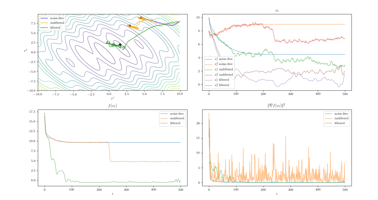
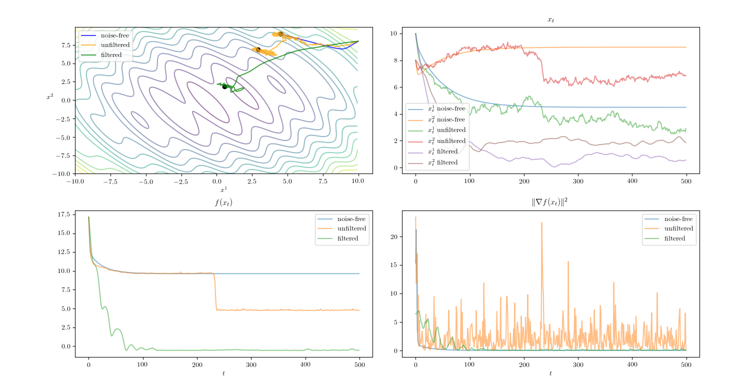
The function f𝑓f is approximately “bowl-shaped” and has many suboptimal local minima which can trap the optimization dynamics. The results for the SGD dynamics are in Figure 1, with the momentum and RMSProp results in Figure 5 of Appendix B.

In Figure 1, we see that the noiseless dynamics did indeed get trapped in a local minimum. For the noisy gradient, the gradient noise actually had a “hill-climbing” effect, but ultimately this too was trapped by a local minimum. We see that the filtered dynamics were able to avoid the “bad” local minima of the first two versions and overall performed much better in terms of minimization and stability.
Refer to caption
Figure 1: Optimization of the function f(x1,x2)𝑓superscript𝑥1superscript𝑥2f(x^{1},x^{2}) in (27) via the dynamics ordinary SGD algorithm. The stepsize was held constant at αt=0.1subscript𝛼𝑡0.1\alpha_{t}=0.1 and the algorithm was run for T=500𝑇500T=500 iterations.

6.2 Parameter Fitting with Black Box Variational Inference

In this experiment, we approximated a two-dimensional target distribution with a two-dimensional Gaussian which has a diagonal covariance. Specifically we approximated

p(z)exp(ϕ(y1.35)+ϕ(xey)),proportional-to𝑝𝑧italic-ϕ𝑦1.35italic-ϕ𝑥superscript𝑒𝑦p(z)\propto\exp\left(\phi\left(\frac{y}{1.35}\right)+\phi\left(\frac{x}{e^{y}}\right)\right),

with z=[x,y]𝑧𝑥𝑦z=[x,y] where ϕitalic-ϕ\phi is the log-normal p.d.f., by the variational family

q(z|λ)=𝒩(z|μ,Σ),λ=(μ,Σ)formulae-sequence𝑞conditional𝑧𝜆𝒩conditional𝑧𝜇Σ𝜆𝜇Σq(z|\lambda)=\mathcal{N}\left(z|\mu,\Sigma\right),~{}~{}~{}\lambda=(\mu,\Sigma)

where μ2,Σ2×2()formulae-sequence𝜇superscript2Σsubscript22\mu\in\mathds{R}^{2},~{}\Sigma\in\mathcal{M}_{2\times 2}(\mathds{R}) and ΣΣ\Sigma is restricted to be diagonal.

We used Black Box Variational Inference (BBVI) Ranganath \BOthers. (\APACyear2013) to optimize a stochastic estimate of the evidence lower bound (ELBO)

(λ)=Eq(|λ)[logp(x,z)logq(z|λ)]1Si=1S[logp(x,zi)logq(zi|λ)];ziq(|λ)\mathcal{L}(\lambda)=E_{q(\cdot|\lambda)}[\log p(x,z)-\log q(z|\lambda)]\approx\frac{1}{S}\sum_{i=1}^{S}[\log p(x,z_{i})-\log q(z_{i}|\lambda)];~{}~{}~{}z_{i}\sim q(\cdot|\lambda)

This objective function was maximized over λ𝜆\lambda using with the gradients coming from backpropagation via the reparameterization trick Kingma \BOthers. (\APACyear2015). The gradient λsubscript𝜆\nabla_{\lambda}\mathcal{L} is necessarily stochastic since it is a Monte Carlo approximation of an expectation. In our experiment, we used the extreme case of a single sample from q(|λ)q(\cdot|\lambda) (i.e. S=1𝑆1S=1) to approximate the expectation.

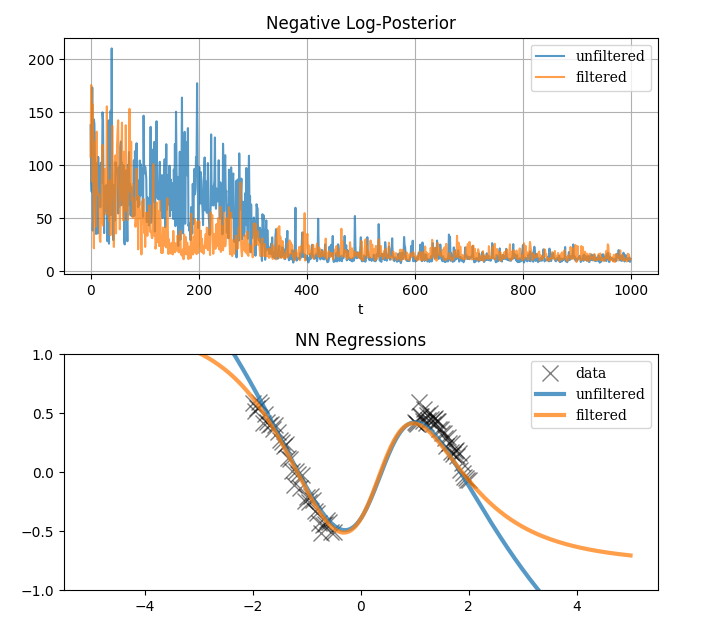
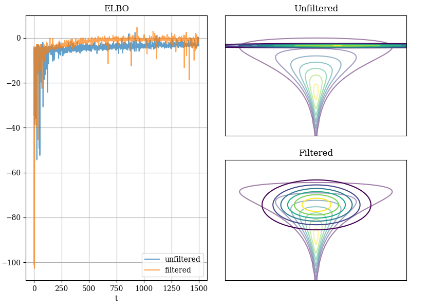
In Figure 2, we see a comparison between unfiltered and filtered results for the BBVI problem above. We used the RMSProp dynamics (24) to maximize (λ)𝜆\mathcal{L}(\lambda). The results illustrate the negative effect that high gradient variance can have on optimization performance.

Of course, one could improve the variance of the unfiltered dynamics by using more samples to estimate the objective; in this case, the performance of the filtered and unfiltered algorithms is similar. However, when a large number of samples is unavailable or impractical, filtering is a good way to improve performance.
Refer to caption
Figure 2: Using BBVI to fit a multivariate normal approximation to a non-Gaussian target. The algorithm uses the reparameterization trick Kingma \BOthers. (\APACyear2015) and the automatic differentiation Python package Autograd Maclaurin \BOthers. (\APACyear2018) to maximize the evidence lower-bound (ELBO) of the variational objective. The ELBO is estimated using a single sample from the variational approximation. The algorithm is run for T=1500𝑇1500T=1500 steps using RMSProp.

6.3 Minibatch Neural Network Training

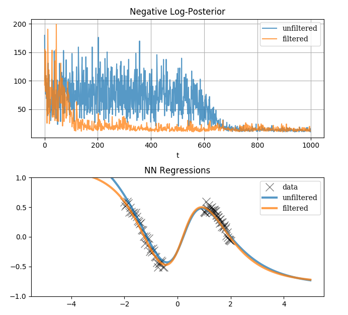
In this experiment, we trained a simple multi-layer perceptron (MLP) to perform a 1-d regression task using minibatches to approximate the loss function. In particular, we used samples from 0.5cos(x)0.5𝑥0.5\cos(x) which were corrupted by additive Gaussian noise and unequally sampled, and whose inputs were scaled and shifted. We used N=80𝑁80N=80 data points, and a batch-size of 8, with randomly sampled batches from the whole data set. We also tested two architectures, layer sizes (1,4,4,1) and (1,20,20,1), to study the effect of dimensionality on the performance of the algorithm. The former is a 33-dimensional problem, and the latter is 481-dimensional.

In Figure 3, we see the improvement that filtering contributes to the optimization performance. In both cases, the filtered algorithm reached a local minimum in significantly fewer algorithm iterations (approx 7x for the small network and 2x for the large network). Both algorithms did converge to similar log-posteriors, and exhibited stability in their minima.
Refer to caption Refer to caption
(a) (b)
Figure 3: Comparison of MLP regression performance. All examples use 1000 iterations, a batch-size of 8 from a sample size of 80, and a stepsize αt=0.011.001tsubscript𝛼𝑡0.01superscript1.001𝑡\alpha_{t}=0.01\cdot 1.001^{-t}. (a): Using layer sizes (1,4,4,1). (b): Using layer sizes (1,20,20,1).

6.4 MNIST Classifier

We studied the use of the Distributed KGD algorithm from Section 4 to classify MNIST digits LeCun (\APACyear1998) using the full-size dataset. We used a vanilla MLP classifier with layer sizes (748, 10, 10, 10). These small sizes were chosen to fit the computational limitations of the testing environment. Even with this relatively small network, training represents a 7,980-dimensional problem, over 10x the size of the problem in Section 6.3. Hence, the Distributed KGD algorithm (Algorithm 2) was required for this task to be completed in reasonable time.

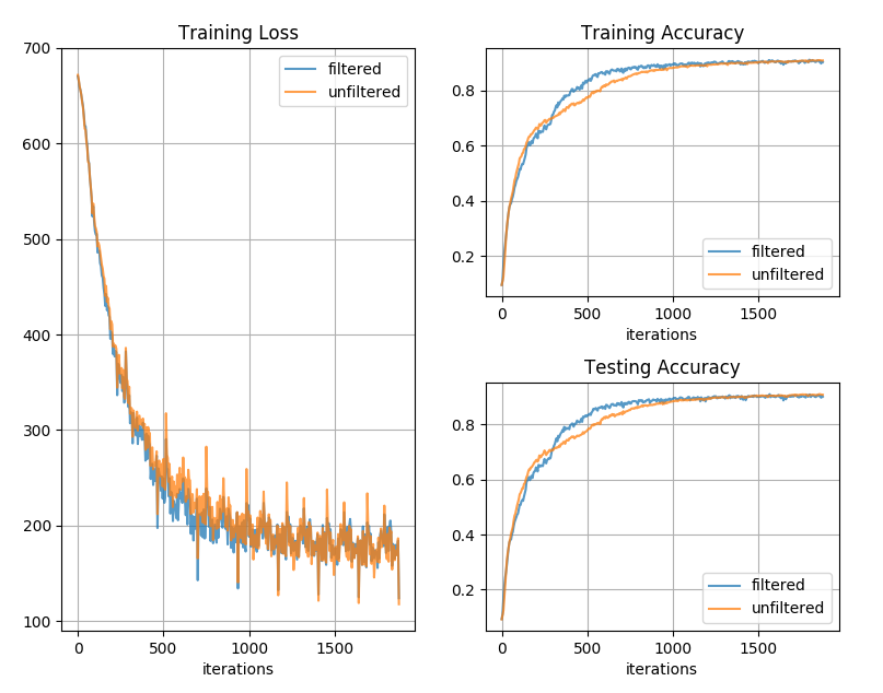
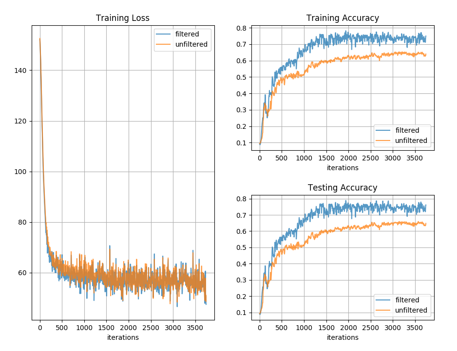
We compared the regular and filtered Distributed RMSProp in two different regimes: small-batch (batch-size 32) and large-batch (batch-size 256). This allowed us to compare the performance of these algorithms in the presence of high- and low-noise gradients respectively. See Figure 4 for the results.

We see that the Distributed KGD algorithm has equal optimization performance in the presence of low gradient variance, but significantly outperforms in the high-variance regime. In the former case, both algorithms achieve approx. 0.9 out-of-sample accuracy, which is reasonable considering the small size of the network. In the high-variance regime, the filtered optimization’s accuracy plateaus significantly higher (approx 0.75) than the unfiltered version (approx 0.65) for the same number of steps. This suggests that the high variance in the gradient estimate caused the unfiltered optimization to converge to a worse local minimum in terms of accuracy. This behaviour can also be seen in Figure 1.
Refer to caption Refer to caption
(a) (b)
Figure 4: Comparison of MNIST classification performance. Both tests use a stepsize of 0.001, and γ=0.9𝛾0.9\gamma=0.9 to train a (784, 10, 10, 10) network. The filtered version uses a sub-vector size of D=50𝐷50D=50. (a): Batch-size 32 with 2 epochs (3,800 steps). (b): Batch-size 256 with 8 epochs (1880 steps).

7 Conclusions

In this work, we have shown how to achieve superior performance in a variety of stochastic optimization problems through the application of Kalman filters to stochastic gradient descent. We provided a theoretical justification for the properties of these new stochastic optimization algorithms, and proposed methods for dealing with high-dimensional problems. We also demonstrated this algorithm’s superior per-iteration efficiency on a variety of optimization and machine learning tasks.

Acknowledgments

We would like to thank Serdar Yüksel and Graeme Baker for their time and insightful feedback during the development this paper.

References

  • Akyildiz \BOthers. (\APACyear2018) \APACinsertmetastarakyildiz2018incremental{APACrefauthors}Akyildiz, Ö\BPBID., Elvira, V.\BCBL \BBA Míguez, J.  \APACrefYearMonthDay2018. \BBOQ\APACrefatitleThe incremental proximal method: A probabilistic perspective The incremental proximal method: A probabilistic perspective.\BBCQ \BIn \APACrefbtitle2018 IEEE International Conference on Acoustics, Speech and Signal Processing (ICASSP) 2018 ieee international conference on acoustics, speech and signal processing (icassp) (\BPGS 4279–4283). \PrintBackRefs\CurrentBib
  • Andrychowicz \BOthers. (\APACyear2016) \APACinsertmetastarandrychowicz2016learning{APACrefauthors}Andrychowicz, M., Denil, M., Gomez, S., Hoffman, M\BPBIW., Pfau, D., Schaul, T.\BDBLDe Freitas, N.  \APACrefYearMonthDay2016. \BBOQ\APACrefatitleLearning to learn by gradient descent by gradient descent Learning to learn by gradient descent by gradient descent.\BBCQ \BIn \APACrefbtitleAdvances in Neural Information Processing Systems Advances in neural information processing systems (\BPGS 3981–3989). \PrintBackRefs\CurrentBib
  • Bertsekas \BBA Tsitsiklis (\APACyear2000) \APACinsertmetastarbertsekas2000gradient{APACrefauthors}Bertsekas, D\BPBIP.\BCBT \BBA Tsitsiklis, J\BPBIN.  \APACrefYearMonthDay2000. \BBOQ\APACrefatitleGradient convergence in gradient methods with errors Gradient convergence in gradient methods with errors.\BBCQ \APACjournalVolNumPagesSIAM Journal on Optimization103627–642. \PrintBackRefs\CurrentBib
  • Bittner \BBA Pronzato (\APACyear2004) \APACinsertmetastarbittner2004kalman{APACrefauthors}Bittner, B.\BCBT \BBA Pronzato, L.  \APACrefYearMonthDay2004. \BBOQ\APACrefatitleKalman filtering in stochastic gradient algorithms: construction of a stopping rule Kalman filtering in stochastic gradient algorithms: construction of a stopping rule.\BBCQ \BIn \APACrefbtitle2004 IEEE International Conference on Acoustics, Speech, and Signal Processing 2004 ieee international conference on acoustics, speech, and signal processing (\BPGS ii–709). \PrintBackRefs\CurrentBib
  • Bottou \BOthers. (\APACyear2018) \APACinsertmetastarbottou2018optimization{APACrefauthors}Bottou, L., Curtis, F\BPBIE.\BCBL \BBA Nocedal, J.  \APACrefYearMonthDay2018. \BBOQ\APACrefatitleOptimization methods for large-scale machine learning Optimization methods for large-scale machine learning.\BBCQ \APACjournalVolNumPagesSIAM Review602223–311. \PrintBackRefs\CurrentBib
  • Cormen \BOthers. (\APACyear2009) \APACinsertmetastarCLRS{APACrefauthors}Cormen, T\BPBIH., Leiserson, C\BPBIE., Rivest, R\BPBIL.\BCBL \BBA Stein, C.  \APACrefYear2009. \APACrefbtitleIntroduction to Algorithms, Third Edition Introduction to algorithms, third edition (\PrintOrdinal3rd \BEd). \APACaddressPublisherThe MIT Press. \PrintBackRefs\CurrentBib
  • Driver (\APACyear2004) \APACinsertmetastardriver2004analysis{APACrefauthors}Driver, B\BPBIK.  \APACrefYearMonthDay2004. \BBOQ\APACrefatitleAnalysis tools with examples Analysis tools with examples.\BBCQ \PrintBackRefs\CurrentBib
  • Duchi \BOthers. (\APACyear2011) \APACinsertmetastarduchi2011adaptive{APACrefauthors}Duchi, J., Hazan, E.\BCBL \BBA Singer, Y.  \APACrefYearMonthDay2011. \BBOQ\APACrefatitleAdaptive subgradient methods for online learning and stochastic optimization Adaptive subgradient methods for online learning and stochastic optimization.\BBCQ \APACjournalVolNumPagesJournal of Machine Learning Research12Jul2121–2159. \PrintBackRefs\CurrentBib
  • Grathwohl \BOthers. (\APACyear2017) \APACinsertmetastargrathwohl2017backpropagation{APACrefauthors}Grathwohl, W., Choi, D., Wu, Y., Roeder, G.\BCBL \BBA Duvenaud, D.  \APACrefYearMonthDay2017. \BBOQ\APACrefatitleBackpropagation through the void: Optimizing control variates for black-box gradient estimation Backpropagation through the void: Optimizing control variates for black-box gradient estimation.\BBCQ \APACjournalVolNumPagesarXiv preprint arXiv:1711.00123. \PrintBackRefs\CurrentBib
  • Huang \BOthers. (\APACyear2011) \APACinsertmetastarhuang2011accelerating{APACrefauthors}Huang, M\BHBIY., Wei, S\BHBIC., Huang, B.\BCBL \BBA Chang, Y\BHBIL.  \APACrefYearMonthDay2011. \BBOQ\APACrefatitleAccelerating the Kalman Filter on a GPU Accelerating the kalman filter on a gpu.\BBCQ \BIn \APACrefbtitle2011 IEEE 17th International Conference on Parallel and Distributed Systems 2011 ieee 17th international conference on parallel and distributed systems (\BPGS 1016–1020). \PrintBackRefs\CurrentBib
  • Jazwinski (\APACyear2007) \APACinsertmetastarjazwinski2007stochastic{APACrefauthors}Jazwinski, A.  \APACrefYear2007. \APACrefbtitleStochastic Processes and Filtering Theory Stochastic processes and filtering theory. \APACaddressPublisherDover Publications, Incorporated. {APACrefURL} https://books.google.ca/books?id=cZzKswEACAAJ \PrintBackRefs\CurrentBib
  • Kalman (\APACyear1960) \APACinsertmetastarKalman1960{APACrefauthors}Kalman, R\BPBIE.  \APACrefYearMonthDay1960. \BBOQ\APACrefatitleA New Approach to Linear Filtering and Prediction Problems A new approach to linear filtering and prediction problems.\BBCQ \APACjournalVolNumPagesTransactions of the ASME–Journal of Basic Engineering82Series D35–45. \PrintBackRefs\CurrentBib
  • Kingma \BBA Ba (\APACyear2014) \APACinsertmetastarkingma2014adam{APACrefauthors}Kingma, D\BPBIP.\BCBT \BBA Ba, J.  \APACrefYearMonthDay2014. \BBOQ\APACrefatitleAdam: A method for stochastic optimization Adam: A method for stochastic optimization.\BBCQ \APACjournalVolNumPagesarXiv preprint arXiv:1412.6980. \PrintBackRefs\CurrentBib
  • Kingma \BOthers. (\APACyear2015) \APACinsertmetastarkingma2015variational{APACrefauthors}Kingma, D\BPBIP., Salimans, T.\BCBL \BBA Welling, M.  \APACrefYearMonthDay2015. \BBOQ\APACrefatitleVariational dropout and the local reparameterization trick Variational dropout and the local reparameterization trick.\BBCQ \BIn \APACrefbtitleAdvances in Neural Information Processing Systems Advances in neural information processing systems (\BPGS 2575–2583). \PrintBackRefs\CurrentBib
  • Lax (\APACyear2014) \APACinsertmetastarlax2014linear{APACrefauthors}Lax, P.  \APACrefYear2014. \APACrefbtitleLinear algebra and its applications Linear algebra and its applications. \APACaddressPublisherWiley. {APACrefURL} https://books.google.ca/books?id=RzJZAQAACAAJ \PrintBackRefs\CurrentBib
  • LeCun (\APACyear1998) \APACinsertmetastarlecun1998mnist{APACrefauthors}LeCun, Y.  \APACrefYearMonthDay1998. \BBOQ\APACrefatitleThe MNIST database of handwritten digits The mnist database of handwritten digits.\BBCQ \APACjournalVolNumPageshttp://yann. lecun. com/exdb/mnist/. \PrintBackRefs\CurrentBib
  • Maclaurin \BOthers. (\APACyear2018) \APACinsertmetastarautograd{APACrefauthors}Maclaurin, D., Duvenaud, D., Johnson, M.\BCBL \BBA Townsend, J.  \APACrefYearMonthDay2018. \APACrefbtitleAutograd. Autograd. \APAChowpublishedhttps://github.com/HIPS/autograd/. \PrintBackRefs\CurrentBib
  • Mandt \BBA Blei (\APACyear2014) \APACinsertmetastarNIPS2014_5557{APACrefauthors}Mandt, S.\BCBT \BBA Blei, D.  \APACrefYearMonthDay2014. \BBOQ\APACrefatitleSmoothed Gradients for Stochastic Variational Inference Smoothed gradients for stochastic variational inference.\BBCQ \BIn Z. Ghahramani, M. Welling, C. Cortes, N\BPBID. Lawrence\BCBL \BBA K\BPBIQ. Weinberger (\BEDS), \APACrefbtitleAdvances in Neural Information Processing Systems 27 Advances in neural information processing systems 27 (\BPGS 2438–2446). \APACaddressPublisherCurran Associates, Inc. {APACrefURL} http://papers.nips.cc/paper/5557-smoothed-gradients-for-stochastic-variational-inference.pdf \PrintBackRefs\CurrentBib
  • Nesterov (\APACyear1983) \APACinsertmetastarnesterov1983method{APACrefauthors}Nesterov, Y\BPBIE.  \APACrefYearMonthDay1983. \BBOQ\APACrefatitleA method for solving the convex programming problem with convergence rate O (1/k^ 2) A method for solving the convex programming problem with convergence rate o (1/k^ 2).\BBCQ \BIn \APACrefbtitleDokl. Akad. Nauk SSSR Dokl. akad. nauk sssr (\BVOL 269, \BPGS 543–547). \PrintBackRefs\CurrentBib
  • Patel (\APACyear2016) \APACinsertmetastarpatel2016kalman{APACrefauthors}Patel, V.  \APACrefYearMonthDay2016. \BBOQ\APACrefatitleKalman-based stochastic gradient method with stop condition and insensitivity to conditioning Kalman-based stochastic gradient method with stop condition and insensitivity to conditioning.\BBCQ \APACjournalVolNumPagesSIAM Journal on Optimization2642620–2648. \PrintBackRefs\CurrentBib
  • Qian (\APACyear1999) \APACinsertmetastarqian1999momentum{APACrefauthors}Qian, N.  \APACrefYearMonthDay1999. \BBOQ\APACrefatitleOn the momentum term in gradient descent learning algorithms On the momentum term in gradient descent learning algorithms.\BBCQ \APACjournalVolNumPagesNeural networks121145–151. \PrintBackRefs\CurrentBib
  • Ranganath \BOthers. (\APACyear2013) \APACinsertmetastarranganath2013black{APACrefauthors}Ranganath, R., Gerrish, S.\BCBL \BBA Blei, D\BPBIM.  \APACrefYearMonthDay2013. \BBOQ\APACrefatitleBlack box variational inference Black box variational inference.\BBCQ \APACjournalVolNumPagesarXiv preprint arXiv:1401.0118. \PrintBackRefs\CurrentBib
  • Reddi \BOthers. (\APACyear2018) \APACinsertmetastarreddi2018convergence{APACrefauthors}Reddi, S\BPBIJ., Kale, S.\BCBL \BBA Kumar, S.  \APACrefYearMonthDay2018. \BBOQ\APACrefatitleOn the convergence of adam and beyond On the convergence of adam and beyond.\BBCQ \PrintBackRefs\CurrentBib
  • Robbins \BBA Monro (\APACyear1985) \APACinsertmetastarrobbins1985stochastic{APACrefauthors}Robbins, H.\BCBT \BBA Monro, S.  \APACrefYearMonthDay1985. \BBOQ\APACrefatitleA stochastic approximation method A stochastic approximation method.\BBCQ \BIn \APACrefbtitleHerbert Robbins Selected Papers Herbert robbins selected papers (\BPGS 102–109). \APACaddressPublisherSpringer. \PrintBackRefs\CurrentBib
  • Roeder \BOthers. (\APACyear2017) \APACinsertmetastarroeder2017sticking{APACrefauthors}Roeder, G., Wu, Y.\BCBL \BBA Duvenaud, D\BPBIK.  \APACrefYearMonthDay2017. \BBOQ\APACrefatitleSticking the landing: Simple, lower-variance gradient estimators for variational inference Sticking the landing: Simple, lower-variance gradient estimators for variational inference.\BBCQ \BIn \APACrefbtitleAdvances in Neural Information Processing Systems Advances in neural information processing systems (\BPGS 6925–6934). \PrintBackRefs\CurrentBib
  • Särkkä (\APACyear2013) \APACinsertmetastarsarkka2013bayesian{APACrefauthors}Särkkä, S.  \APACrefYear2013. \APACrefbtitleBayesian filtering and smoothing Bayesian filtering and smoothing (\BVOL 3). \APACaddressPublisherCambridge University Press. \PrintBackRefs\CurrentBib
  • Schraudolph (\APACyear1999) \APACinsertmetastarschraudolph1999local{APACrefauthors}Schraudolph, N\BPBIN.  \APACrefYearMonthDay1999. \BBOQ\APACrefatitleLocal gain adaptation in stochastic gradient descent Local gain adaptation in stochastic gradient descent.\BBCQ \PrintBackRefs\CurrentBib
  • Tieleman \BBA Hinton (\APACyear2012) \APACinsertmetastarTieleman2012{APACrefauthors}Tieleman, T.\BCBT \BBA Hinton, G.  \APACrefYearMonthDay2012. \APACrefbtitleLecture 6.5—RmsProp: Divide the gradient by a running average of its recent magnitude. Lecture 6.5—RmsProp: Divide the gradient by a running average of its recent magnitude. \APAChowpublishedCOURSERA: Neural Networks for Machine Learning. \PrintBackRefs\CurrentBib
  • Tseng (\APACyear1998) \APACinsertmetastartseng1998incremental{APACrefauthors}Tseng, P.  \APACrefYearMonthDay1998. \BBOQ\APACrefatitleAn incremental gradient (-projection) method with momentum term and adaptive stepsize rule An incremental gradient (-projection) method with momentum term and adaptive stepsize rule.\BBCQ \APACjournalVolNumPagesSIAM Journal on Optimization82506–531. \PrintBackRefs\CurrentBib
  • van Handel (\APACyear2010) \APACinsertmetastarvan2010nonlinear{APACrefauthors}van Handel, R.  \APACrefYearMonthDay2010. \BBOQ\APACrefatitleNonlinear filtering and systems theory Nonlinear filtering and systems theory.\BBCQ \BIn \APACrefbtitleProceedings of the 19th International Symposium on Mathematical Theory of Networks and Systems (MTNS semi-plenary paper). Proceedings of the 19th international symposium on mathematical theory of networks and systems (mtns semi-plenary paper). \PrintBackRefs\CurrentBib
  • Wang \BOthers. (\APACyear2013) \APACinsertmetastarwang2013variance{APACrefauthors}Wang, C., Chen, X., Smola, A\BPBIJ.\BCBL \BBA Xing, E\BPBIP.  \APACrefYearMonthDay2013. \BBOQ\APACrefatitleVariance reduction for stochastic gradient optimization Variance reduction for stochastic gradient optimization.\BBCQ \BIn \APACrefbtitleAdvances in Neural Information Processing Systems Advances in neural information processing systems (\BPGS 181–189). \PrintBackRefs\CurrentBib

Appendix A Proofs

A.1 Filtering Proofs

The Kalman filtering dynamics (7)(12)italic-(7italic-)italic-(12italic-)\eqref{eq:kal1}-\eqref{eq:kal6} form a discrete-time LTV dynamical system, hence to study this system we will use the language and tools of LTV systems theory. In particular, the results below establish the asymptotic properties of the Kalman filter for general discrete-time LTV dynamical system

{xt+1=Atxt+Γtwtyt=Ctxt+vt;xtm,wtm,ytp.formulae-sequencecasessubscript𝑥𝑡1absentsubscript𝐴𝑡subscript𝑥𝑡subscriptΓ𝑡subscript𝑤𝑡subscript𝑦𝑡absentsubscript𝐶𝑡subscript𝑥𝑡subscript𝑣𝑡subscript𝑥𝑡superscript𝑚formulae-sequencesubscript𝑤𝑡superscript𝑚subscript𝑦𝑡superscript𝑝\left\{\begin{array}[]{r l}x_{t+1}&=A_{t}x_{t}+\Gamma_{t}w_{t}\\ y_{t}&=C_{t}x_{t}+v_{t}\end{array}\right.;~{}~{}~{}x_{t}\in\mathds{R}^{m},~{}w_{t}\in\mathds{R}^{m},~{}y_{t}\in\mathds{R}^{p}. (28)

where wt𝒩(0,Qt)similar-tosubscript𝑤𝑡𝒩0subscript𝑄𝑡w_{t}\sim\mathcal{N}(0,Q_{t}) and vt𝒩(0,Rt)similar-tosubscript𝑣𝑡𝒩0subscript𝑅𝑡v_{t}\sim\mathcal{N}(0,R_{t}) with Qt,Rtsubscript𝑄𝑡subscript𝑅𝑡Q_{t},R_{t} positive definite matrices.

Definition 2.

The for (28), observability matrix is

𝒪(t,1)=i=1tΦT(i,t)CiTRi1CiΦ(i,t)𝒪𝑡1superscriptsubscript𝑖1𝑡superscriptΦ𝑇𝑖𝑡superscriptsubscript𝐶𝑖𝑇superscriptsubscript𝑅𝑖1subscript𝐶𝑖Φ𝑖𝑡\mathcal{O}(t,1)=\sum_{i=1}^{t}\Phi^{T}(i,t)C_{i}^{T}R_{i}^{-1}C_{i}\Phi(i,t)

and the controllability matrix is

𝒞(t,0)=i=0t1Φ(t,i+1)ΓiQiΓiTΦT(t,i+1)𝒞𝑡0superscriptsubscript𝑖0𝑡1Φ𝑡𝑖1subscriptΓ𝑖subscript𝑄𝑖superscriptsubscriptΓ𝑖𝑇superscriptΦ𝑇𝑡𝑖1\mathcal{C}(t,0)=\sum_{i=0}^{t-1}\Phi(t,i+1)\Gamma_{i}Q_{i}\Gamma_{i}^{T}\Phi^{T}(t,i+1)

where Φ(t,s)Φ𝑡𝑠\Phi(t,s) is the state transition matrix of (28), i.e. the solution to the homogeneous state equation.

Definition 3.

The Kalman filtered dynamics of (28) are uniformly completely observable if No>0subscript𝑁𝑜subscriptabsent0\exists N_{o}\in\mathds{Z}_{>0} and α,β>0𝛼𝛽subscriptabsent0\alpha,\beta\in\mathds{R}_{>0} s.t.

0<αI𝒪(t,tNo)βItNo0𝛼𝐼𝒪𝑡𝑡subscript𝑁𝑜𝛽𝐼for-all𝑡subscript𝑁𝑜0<\alpha I\leq\mathcal{O}(t,t-N_{o})\leq\beta I~{}~{}~{}\forall t\geq N_{o}

and uniformly completely controllable if Nc>0subscript𝑁𝑐subscriptabsent0\exists N_{c}\in\mathds{Z}_{>0} and α,β>0superscript𝛼superscript𝛽subscriptabsent0\alpha^{\prime},\beta^{\prime}\in\mathds{R}_{>0} s.t.

0<αI𝒞(t,tNc)βItNc.0superscript𝛼𝐼𝒞𝑡𝑡subscript𝑁𝑐superscript𝛽𝐼for-all𝑡subscript𝑁𝑐0<\alpha^{\prime}I\leq\mathcal{C}(t,t-N_{c})\leq\beta^{\prime}I~{}~{}~{}\forall t\geq N_{c}.

Note that stability of the system’s internal dynamics does not necessarily imply stability of the filter van Handel (\APACyear2010). The below theorems, which are from Jazwinski (\APACyear2007), will be used to establish Theorem 1 in terms of uniform complete observability and controllability.

Theorem 3 (Kalman Filter Stability).

If (28) is uniformly completely observable and uniformly completely controllable, then the discrete-time Kalman filter is uniformly asymptotically stable.

Proof.

See Jazwinski (\APACyear2007) Theorem 7.4 p.240. ∎

Theorem 4 (Kalman Filter Error Boundedness).

If (28) is is uniformly completely observable and uniformly completely controllable, and if P0>0subscript𝑃00P_{0}>0 there exist α,β>0𝛼𝛽subscriptabsent0\alpha,\beta\in\mathds{R}_{>0} and N>0𝑁subscriptabsent0N\in\mathds{Z}_{>0} s.t.

α1+αβIPt|t1+αβαItN.𝛼1𝛼𝛽𝐼subscript𝑃conditional𝑡𝑡1𝛼𝛽𝛼𝐼for-all𝑡𝑁\frac{\alpha}{1+\alpha\beta}I\leq P_{t|t}\leq\frac{1+\alpha\beta}{\alpha}I~{}~{}~{}\forall t\geq N.
Proof.

See Jazwinski (\APACyear2007) Lemmas 7.1 & 7.2 p.234. ∎

Theorem 5 (Kalman Filter Robustness).

Suppose (28) is uniformly completely observable and uniformly completely controllable, and let Pt|t1,Pt|t2subscriptsuperscript𝑃1conditional𝑡𝑡subscriptsuperscript𝑃2conditional𝑡𝑡P^{1}_{t|t},P^{2}_{t|t} be two solutions to the Kalman filter dynamics with initial conditions P01,P020subscriptsuperscript𝑃10subscriptsuperscript𝑃200P^{1}_{0},P^{2}_{0}\geq 0 resp. Then k1,k20subscript𝑘1subscript𝑘2subscriptabsent0\exists k_{1},k_{2}\in\mathds{R}_{\geq 0} s.t.

Pt|t1Pt|t2k1ek2tP01P020normsubscriptsuperscript𝑃1conditional𝑡𝑡subscriptsuperscript𝑃2conditional𝑡𝑡subscript𝑘1superscript𝑒subscript𝑘2𝑡normsubscriptsuperscript𝑃10subscriptsuperscript𝑃200\|P^{1}_{t|t}-P^{2}_{t|t}\|\leq k_{1}e^{-k_{2}t}\|P^{1}_{0}-P^{2}_{0}\|\to 0

as t𝑡t\to\infty.

Proof.

See Jazwinski (\APACyear2007) Theorem 7.5 p.242. ∎

With the conditions for the stability of the Kalman filter above, we will show that Assumption 1 implies uniform complete observability and controllability for (6), and this implies Theorem 1.

Lemma 1.

Let tMtmaps-to𝑡subscript𝑀𝑡t\mapsto M_{t} be a n×n𝑛𝑛n\times n, real, positive-definite matrix-valued function. Suppose that det(Mt)=Ktsubscript𝑀𝑡𝐾for-all𝑡\det(M_{t})=K~{}\forall t, and suppose that λ>0superscript𝜆subscriptabsent0\exists\lambda^{*}\in\mathds{R}_{>0} such that λtiλtsubscriptsuperscript𝜆𝑖𝑡superscript𝜆for-all𝑡\lambda^{i}_{t}\leq\lambda^{*}~{}\forall t and every i𝑖i, where λtisubscriptsuperscript𝜆𝑖𝑡\lambda^{i}_{t} are the eigenvalues of Mtsubscript𝑀𝑡M_{t}. Then λλtitsubscript𝜆subscriptsuperscript𝜆𝑖𝑡for-all𝑡\exists\lambda_{*}\leq\lambda^{i}_{t}~{}\forall t and every i𝑖i.

Proof.

Assume WLOG that det(Mt)=1tsubscript𝑀𝑡1for-all𝑡\det(M_{t})=1~{}\forall t. Note that each λti>0subscriptsuperscript𝜆𝑖𝑡0\lambda^{i}_{t}>0 and also that det(Mt)=i=1nλtisubscript𝑀𝑡superscriptsubscriptproduct𝑖1𝑛subscriptsuperscript𝜆𝑖𝑡\det(M_{t})=\prod_{i=1}^{n}\lambda^{i}_{t}. Then consider making λtnsubscriptsuperscript𝜆𝑛𝑡\lambda^{n}_{t} the smallest possible for any choice of λt1,,λtn1subscriptsuperscript𝜆1𝑡subscriptsuperscript𝜆𝑛1𝑡\lambda^{1}_{t},\dots,\lambda^{n-1}_{t} under the constraint that det(Mt)=1subscript𝑀𝑡1\det(M_{t})=1. This obviously occurs when λt1==λtn1=λsubscriptsuperscript𝜆1𝑡subscriptsuperscript𝜆𝑛1𝑡superscript𝜆\lambda^{1}_{t}=\cdots=\lambda^{n-1}_{t}=\lambda^{*}. In this case,

λtn=1λt1λtn1=1(λ)d1.subscriptsuperscript𝜆𝑛𝑡1subscriptsuperscript𝜆1𝑡subscriptsuperscript𝜆𝑛1𝑡1superscriptsuperscript𝜆𝑑1\lambda^{n}_{t}=\frac{1}{\lambda^{1}_{t}\cdots\lambda^{n-1}_{t}}=\frac{1}{(\lambda^{*})^{d-1}}.

Hence λti(λ)(d1)=λsubscriptsuperscript𝜆𝑖𝑡superscriptsuperscript𝜆𝑑1subscript𝜆\lambda^{i}_{t}\geq(\lambda^{*})^{-(d-1)}=\lambda_{*}. ∎

Lemma 2.
  1. (a)

    For an invertible n×n𝑛𝑛n\times n matrix M𝑀M which satisfies MTM<αIsuperscript𝑀𝑇𝑀𝛼𝐼M^{T}M<\alpha I we have

    (Mn)T(Mn)<αnIsuperscriptsuperscript𝑀𝑛𝑇superscript𝑀𝑛superscript𝛼𝑛𝐼(M^{n})^{T}(M^{n})<\alpha^{n}I
  2. (b)

    Suppose that U,V𝑈𝑉U,V are two n×n𝑛𝑛n\times n positive definite matrices s.t. 0<U<V0𝑈𝑉0<U<V. Then we have

    U1>V1.superscript𝑈1superscript𝑉1U^{-1}>V^{-1}.
  3. (c)

    For a square, invertible matrix M𝑀M, (MMT)1=(M1)TM1superscript𝑀superscript𝑀𝑇1superscriptsuperscript𝑀1𝑇superscript𝑀1(MM^{T})^{-1}=(M^{-1})^{T}M^{-1}.

Proof.
  1. (a)

    Lax (\APACyear2014) Ch 10.1 p.146.

  2. (b)

    Lax (\APACyear2014) Theorem 2, Ch 10.1 p.146

  3. (c)

    Easy to directly verify.

Lemma 3 (KGD Observability and Controllability).

Under Assumption 1, the KGD dynamics (6) are uniformly completely observable and controllable.

Proof.

This proof is organized into three steps: First, we prove uniform complete controllability, then extend the machinery of complete controllability, and finally apply this extended machinery to prove uniform complete observability.

  1. 1.

    We will take Nc=2subscript𝑁𝑐2N_{c}=2. Then ΓtIsubscriptΓ𝑡𝐼\Gamma_{t}\equiv I, Qt=σQI>0tsubscript𝑄𝑡subscript𝜎𝑄𝐼0for-all𝑡Q_{t}=\sigma_{Q}I>0~{}\forall t in the definition above, hence we have

    𝒞(t,t2)=σQI+σQΦ(t,t1)ΦT(t,t1)=σQI+σQAt1At1T.𝒞𝑡𝑡2subscript𝜎𝑄𝐼subscript𝜎𝑄Φ𝑡𝑡1superscriptΦ𝑇𝑡𝑡1subscript𝜎𝑄𝐼subscript𝜎𝑄subscript𝐴𝑡1superscriptsubscript𝐴𝑡1𝑇\mathcal{C}(t,t-2)=\sigma_{Q}I+\sigma_{Q}\Phi(t,t-1)\Phi^{T}(t,t-1)=\sigma_{Q}I+\sigma_{Q}A_{t-1}A_{t-1}^{T}.

    It suffices to prove the case when σQ=1subscript𝜎𝑄1\sigma_{Q}=1, and to prove the uniform boundedness of the second term. We will first show that vTAt1At1Tv=At1Tv2superscript𝑣𝑇subscript𝐴𝑡1superscriptsubscript𝐴𝑡1𝑇𝑣superscriptnormsuperscriptsubscript𝐴𝑡1𝑇𝑣2v^{T}A_{t-1}A_{t-1}^{T}v=\|A_{t-1}^{T}v\|^{2} has upper bound which does not depend on t𝑡t for an arbitrary v2n𝑣superscript2𝑛v\in\mathds{R}^{2n}. We have that

    At1T=[I0αt1I]superscriptsubscript𝐴𝑡1𝑇matrix𝐼0subscript𝛼𝑡1𝐼A_{t-1}^{T}=\begin{bmatrix}I&0\\ -\alpha_{t-1}&I\end{bmatrix}

    hence writing v=[v1T,v2T]T𝑣superscriptsuperscriptsubscript𝑣1𝑇superscriptsubscript𝑣2𝑇𝑇v=[v_{1}^{T},v_{2}^{T}]^{T} and using x+y22x2+2y2superscriptnorm𝑥𝑦22superscriptnorm𝑥22superscriptnorm𝑦2\|x+y\|^{2}\leq 2\|x\|^{2}+2\|y\|^{2}, we have that

    At1Tv2superscriptnormsuperscriptsubscript𝐴𝑡1𝑇𝑣2\displaystyle\|A_{t-1}^{T}v\|^{2} =v12+v2αt1v12absentsuperscriptnormsubscript𝑣12superscriptnormsubscript𝑣2subscript𝛼𝑡1subscript𝑣12\displaystyle=\|v_{1}\|^{2}+\|v_{2}-\alpha_{t-1}v_{1}\|^{2}
    v12+2v22+2(αt1)2v12absentsuperscriptnormsubscript𝑣122superscriptnormsubscript𝑣222superscriptsubscript𝛼𝑡12superscriptnormsubscript𝑣12\displaystyle\leq\|v_{1}\|^{2}+2\|v_{2}\|^{2}+2(\alpha_{t-1})^{2}\|v_{1}\|^{2}
    =(1+2αt12)v12+2v22absent12superscriptsubscript𝛼𝑡12superscriptnormsubscript𝑣122superscriptnormsubscript𝑣22\displaystyle=(1+2\alpha_{t-1}^{2})\|v_{1}\|^{2}+2\|v_{2}\|^{2}
    (1+2α)v12+2v22.absent12superscript𝛼superscriptnormsubscript𝑣122superscriptnormsubscript𝑣22\displaystyle\leq(1+2\alpha^{*})\|v_{1}\|^{2}+2\|v_{2}\|^{2}.

    where α=maxtαt<superscript𝛼subscript𝑡subscript𝛼𝑡\alpha^{*}=\max_{t}\alpha_{t}<\infty by assumption. To show the existence of a uniform lower bound, we will appeal to Lemma 1 to show that the spectrum of Φ(t,t1)Φ(t,t1)TΦ𝑡𝑡1Φsuperscript𝑡𝑡1𝑇\Phi(t,t-1)\Phi(t,t-1)^{T} is uniformly lower-bounded, and this implies the required matrix inequality. Indeed, det(At1)=1subscript𝐴𝑡11\det(A_{t-1})=1 so that

    det(Φ(t,t1)Φ(t,t1)T)=det(At1At1T)=1Φ𝑡𝑡1Φsuperscript𝑡𝑡1𝑇subscript𝐴𝑡1superscriptsubscript𝐴𝑡1𝑇1\det(\Phi(t,t-1)\Phi(t,t-1)^{T})=\det(A_{t-1}A_{t-1}^{T})=1 (29)

    and since we have just shown an uniform upper matrix bound (which implies a uniformly upper-bounded spectrum), Lemma 1 implies there is a uniform lower matrix bound which is >0absent0>0.

  2. 2.

    Using the multiplicative property from Lemma 2(a), we can iterate the result for the controllability matrix by conjugating AtTsubscript𝐴𝑡𝑇A_{t-T} with AtT+1,,At1subscript𝐴𝑡𝑇1subscript𝐴𝑡1A_{t-T+1},\dots,A_{t-1} to see that Φ(t,tT)Φ(t,tT)TΦ𝑡𝑡𝑇Φsuperscript𝑡𝑡𝑇𝑇\Phi(t,t-T)\Phi(t,t-T)^{T} is also uniformly bounded above for a fixed T>0𝑇0T>0. The fact that we are conjugating by matrices whose determinants are all 1 allows us to use Lemma 1 again to conclude the existence of a uniform lower bound on Φ(t,tT)Φ(t,tT)TΦ𝑡𝑡𝑇Φsuperscript𝑡𝑡𝑇𝑇\Phi(t,t-T)\Phi(t,t-T)^{T}. Now,

    Φ(tT,t)TΦ(tT,t)=(Φ(t,tT)1)T(Φ(t,tT)1)=(Φ(t,tT)Φ(t,tT)T)1Φsuperscript𝑡𝑇𝑡𝑇Φ𝑡𝑇𝑡superscriptΦsuperscript𝑡𝑡𝑇1𝑇Φsuperscript𝑡𝑡𝑇1superscriptΦ𝑡𝑡𝑇Φsuperscript𝑡𝑡𝑇𝑇1\Phi(t-T,t)^{T}\Phi(t-T,t)=(\Phi(t,t-T)^{-1})^{T}(\Phi(t,t-T)^{-1})=\left(\Phi(t,t-T)\Phi(t,t-T)^{T}\right)^{-1} (30)

    by Lemma 2(c). Then Lemma 2(b) implies the existence of uniform bounds on Φ(tT,t)TΦ(tT,t)Φsuperscript𝑡𝑇𝑡𝑇Φ𝑡𝑇𝑡\Phi(t-T,t)^{T}\Phi(t-T,t).

  3. 3.

    Now, for the observability matrix, consider for a fixed No>0subscript𝑁𝑜0N_{o}>0

    𝒪(t,tNo)=σR1i=tNotΦT(i,t)CiTCiΦ(i,t).𝒪𝑡𝑡subscript𝑁𝑜superscriptsubscript𝜎𝑅1superscriptsubscript𝑖𝑡subscript𝑁𝑜𝑡superscriptΦ𝑇𝑖𝑡superscriptsubscript𝐶𝑖𝑇subscript𝐶𝑖Φ𝑖𝑡\mathcal{O}(t,t-N_{o})=\sigma_{R}^{-1}\sum_{i=t-N_{o}}^{t}\Phi^{T}(i,t)C_{i}^{T}C_{i}\Phi(i,t).

    We will also assume that σR=1subscript𝜎𝑅1\sigma_{R}=1. Thus, by ensuring that Ci=I2n×2nsubscript𝐶𝑖subscript𝐼2𝑛2𝑛C_{i}=I_{2n\times 2n} at least once every Nosubscript𝑁𝑜N_{o} timesteps, one of the matrices in the sum 𝒪(t,tNo)𝒪𝑡𝑡subscript𝑁𝑜\mathcal{O}(t,t-N_{o}) of the form (30) and hence is uniformly bounded above and below. The other terms in the sum are not definite since Cisubscript𝐶𝑖C_{i} is rank-deficient at those times, but they are positive and uniformly bounded, hence the system is uniformly completely observable.

Note that since Nosubscript𝑁𝑜N_{o} is arbitrary, we can make it can be very large. In practice, Nosubscript𝑁𝑜N_{o} can be larger than the total number of timesteps of a run of the algorithm. This is why we have omitted this technical detail from the setup in Section 2.

Lemma 4 (Extended KGD Observability and Controllability).

Under Assumptions 1 and 2, if μt=μsubscript𝜇𝑡𝜇\mu_{t}=\mu in (22) and γt=γsubscript𝛾𝑡𝛾\gamma_{t}=\gamma in (25) updates are constant, then the dynamics for (22)-(23) and (25)-(26) are uniformly completely controllable and observable.

Proof.

We need to prove a version of Lemma 3. This lemma uses the facts that AtAtT<αIsubscript𝐴𝑡superscriptsubscript𝐴𝑡𝑇𝛼𝐼A_{t}A_{t}^{T}<\alpha I for some α𝛼\alpha uniformly in t𝑡t, and that the determinant of Atsubscript𝐴𝑡A_{t} is constant. The latter follows immediately by inspection since Atsubscript𝐴𝑡A_{t} is upper triangular. For the uniform upper-bound, consider first momentum: for v=[v1T,v2T,v3T]T3n𝑣superscriptsuperscriptsubscript𝑣1𝑇superscriptsubscript𝑣2𝑇superscriptsubscript𝑣3𝑇𝑇superscript3𝑛v=[v_{1}^{T},v_{2}^{T},v_{3}^{T}]^{T}\in\mathds{R}^{3n} we have

At1Tv2superscriptnormsuperscriptsubscript𝐴𝑡1𝑇𝑣2\displaystyle\|A_{t-1}^{T}v\|^{2} =v12+αt1μv1+μv22+αt1(1μ)v1(1μ)v2+v32absentsuperscriptnormsubscript𝑣12superscriptnormsubscript𝛼𝑡1𝜇subscript𝑣1𝜇subscript𝑣22superscriptnormsubscript𝛼𝑡11𝜇subscript𝑣11𝜇subscript𝑣2subscript𝑣32\displaystyle=\|v_{1}\|^{2}+\|\alpha_{t-1}\mu v_{1}+\mu v_{2}\|^{2}+\|-\alpha_{t-1}(1-\mu)v_{1}-(1-\mu)v_{2}+v_{3}\|^{2}
v12+2(αt1μ)2v12+2μ2v22+3(αt1(1μ))2v12+3(1μ)2v22+3v32absentsuperscriptnormsubscript𝑣122superscriptsubscript𝛼𝑡1𝜇2superscriptnormsubscript𝑣122superscript𝜇2superscriptnormsubscript𝑣223superscriptsubscript𝛼𝑡11𝜇2superscriptnormsubscript𝑣123superscript1𝜇2superscriptnormsubscript𝑣223superscriptnormsubscript𝑣32\displaystyle\leq\|v_{1}\|^{2}+2(\alpha_{t-1}\mu)^{2}\|v_{1}\|^{2}+2\mu^{2}\|v_{2}\|^{2}+3(\alpha_{t-1}(1-\mu))^{2}\|v_{1}\|^{2}+3(1-\mu)^{2}\|v_{2}\|^{2}+3\|v_{3}\|^{2}
=[1+2(αt1μ)2+3(αt1(1μ))2]v12+[2μ2+3(1μ)2]v22+3v32absentdelimited-[]12superscriptsubscript𝛼𝑡1𝜇23superscriptsubscript𝛼𝑡11𝜇2superscriptnormsubscript𝑣12delimited-[]2superscript𝜇23superscript1𝜇2superscriptnormsubscript𝑣223superscriptnormsubscript𝑣32\displaystyle=[1+2(\alpha_{t-1}\mu)^{2}+3(\alpha_{t-1}(1-\mu))^{2}]\|v_{1}\|^{2}+[2\mu^{2}+3(1-\mu)^{2}]\|v_{2}\|^{2}+3\|v_{3}\|^{2}
[1+2(αμ)2+3(α(1μ))2]v12+[2μ2+3(1μ)2]v22+3v32absentdelimited-[]12superscriptsuperscript𝛼𝜇23superscriptsuperscript𝛼1𝜇2superscriptnormsubscript𝑣12delimited-[]2superscript𝜇23superscript1𝜇2superscriptnormsubscript𝑣223superscriptnormsubscript𝑣32\displaystyle\leq[1+2(\alpha^{*}\mu)^{2}+3(\alpha^{*}(1-\mu))^{2}]\|v_{1}\|^{2}+[2\mu^{2}+3(1-\mu)^{2}]\|v_{2}\|^{2}+3\|v_{3}\|^{2}

with α=maxtαt<superscript𝛼subscript𝑡subscript𝛼𝑡\alpha^{*}=\max_{t}\alpha_{t}<\infty.

For RMSProp, we proceed similarly:

At1Tv2superscriptnormsuperscriptsubscript𝐴𝑡1𝑇𝑣2\displaystyle\|A_{t-1}^{T}v\|^{2} =v12+γv22+αt1diag(βt1)v1+(1γ)diag(f(xt1))v2+v32absentsuperscriptnormsubscript𝑣12superscriptnorm𝛾subscript𝑣22superscriptnormsubscript𝛼𝑡1diagsubscript𝛽𝑡1subscript𝑣11𝛾diag𝑓subscript𝑥𝑡1subscript𝑣2subscript𝑣32\displaystyle=\|v_{1}\|^{2}+\|\gamma v_{2}\|^{2}+\|-\alpha_{t-1}\mathrm{diag}(\beta_{t-1})v_{1}+(1-\gamma)\mathrm{diag}(\nabla f(x_{t-1}))v_{2}+v_{3}\|^{2}
v12+γ2v22+3αt12diag(βt1)v12()+3(1γ)2diag(f(xt1))v22()+3v32absentsuperscriptnormsubscript𝑣12superscript𝛾2superscriptnormsubscript𝑣223superscriptsubscript𝛼𝑡12subscriptsuperscriptnormdiagsubscript𝛽𝑡1subscript𝑣123superscript1𝛾2subscriptsuperscriptnormdiag𝑓subscript𝑥𝑡1subscript𝑣22absent3superscriptnormsubscript𝑣32\displaystyle\leq\|v_{1}\|^{2}+\gamma^{2}\|v_{2}\|^{2}+3\alpha_{t-1}^{2}\underbrace{\|\mathrm{diag}(\beta_{t-1})v_{1}\|^{2}}_{(*)}+3(1-\gamma)^{2}\underbrace{\|\mathrm{diag}(\nabla f(x_{t-1}))v_{2}\|^{2}}_{(**)}+3\|v_{3}\|^{2}

It remains to show that the terms ()(*) and ()(**) are uniformly bounded above. In the former case, this is true since βt=(rt+1+ε)1subscript𝛽𝑡superscriptsubscript𝑟𝑡1𝜀1\beta_{t}=(\sqrt{r_{t+1}}+\varepsilon)^{-1} and rt+10subscript𝑟𝑡10\sqrt{r_{t+1}}\geq 0. In the latter case, using the Frobenius norm on the matrix diag(f(xt1))diag𝑓subscript𝑥𝑡1\mathrm{diag}(\nabla f(x_{t-1})) we have

diag(f(xt1))v3diag(f(xt1))v3=f(xt1)v3Gv3normdiag𝑓subscript𝑥𝑡1subscript𝑣3normdiag𝑓subscript𝑥𝑡1normsubscript𝑣3norm𝑓subscript𝑥𝑡1normsubscript𝑣3𝐺normsubscript𝑣3\|\mathrm{diag}(\nabla f(x_{t-1}))v_{3}\|\leq\|\mathrm{diag}(\nabla f(x_{t-1}))\|\|v_{3}\|=\|\nabla f(x_{t-1})\|\|v_{3}\|\leq G\|v_{3}\|

where G𝐺G is the uniform bound on f𝑓\nabla f. Hence the rest of the proof of Lemma 3 can be applied to the momentum and RMSProp cases respectively. ∎

A.2 Stochastic Optimization Proofs

For simplicity, to prove the convergence of (19) we prove convergence of the system

{vt+1=(1β)vt+βg(xt;ξt)xt+1=xtαtvt+1casessubscript𝑣𝑡1absent1𝛽subscript𝑣𝑡𝛽𝑔subscript𝑥𝑡subscript𝜉𝑡subscript𝑥𝑡1absentsubscript𝑥𝑡subscript𝛼𝑡subscript𝑣𝑡1\left\{\begin{array}[]{r l}v_{t+1}&=(1-\beta)v_{t}+\beta g(x_{t};\xi_{t})\\ x_{t+1}&=x_{t}-\alpha_{t}v_{t+1}\end{array}\right. (31)

with xn𝑥superscript𝑛x\in\mathds{R}^{n}, β]0,1[\beta\in]0,1[ and appeal to Proposition 2 which implies that we do not lose any generality in doing so.

Proposition 2.
  1. (a)

    If β𝛽\beta from (31) is allowed to vary with time s.t. 0<β<βt<β<10subscript𝛽subscript𝛽𝑡superscript𝛽10<\beta_{*}<\beta_{t}<\beta^{*}<1 then the results of this section hold with βsubscript𝛽\beta_{*} and βsuperscript𝛽\beta^{*} replacing β𝛽\beta appropriately.

  2. (b)

    We can replace β𝛽\beta from (31) by a positive-definite matrix B𝐵B with 0<βI<B<βI<I0subscript𝛽𝐼𝐵superscript𝛽𝐼𝐼0<\beta_{*}I<B<\beta^{*}I<I without materially affecting the results of this section.

Proof.
  1. (a)

    Since we never used the property (1β)+β=11𝛽𝛽1(1-\beta)+\beta=1, we can replace each instance of β𝛽\beta by the appropriate bound βsuperscript𝛽\beta^{*} or βsubscript𝛽\beta_{*} depending on the sign of β𝛽\beta to preserve any inequality, and all finite sums/ products can be bounded by appropriate upper/lower bounds.

  2. (b)

    The matrix B𝐵B (or possibly IB𝐼𝐵I-B as the case may be) defines a new inner product which is re-weighted by B𝐵B. By the equivalence of norms (hence inner products) on nsuperscript𝑛\mathds{R}^{n}, the claim holds.

In the sequel, E[]𝐸delimited-[]E[\cdot] will denote the expectation w.r.t. the joint distribution of the ξs,stsubscript𝜉𝑠𝑠𝑡\xi_{s},~{}s\leq t where t𝑡t is the latest time in the expectation. For convenience, we will restate the necessary assumptions from Section 3 as needed.

Assumption 4 (Same as Assumption 2).

The objective function f:n:𝑓superscript𝑛f:\mathds{R}^{n}\to\mathds{R} is C3superscript𝐶3C^{3}, with uniformly bounded 1st, 2nd, and 3rd derivatives. In particular f𝑓\nabla f is Lipschitz with constant L𝐿L.

Assumption 5 (Same as Assumption 3).

The random variables g(xt,;ξt)g(x_{t},;\xi_{t}) satisfy the following properties

  1. (a)

    E[f(xt)Tg(xt;ξt)]μE[f(xt)2]𝐸delimited-[]𝑓superscriptsubscript𝑥𝑡𝑇𝑔subscript𝑥𝑡subscript𝜉𝑡𝜇𝐸delimited-[]superscriptnorm𝑓subscript𝑥𝑡2E[\nabla f(x_{t})^{T}g(x_{t};\xi_{t})]\geq\mu E[\|\nabla f(x_{t})\|^{2}] for some constant μ>0𝜇0\mu>0 and tfor-all𝑡\forall t;

  2. (b)

    E[g(xt;ξt)2]M+MGE[f(xt)2]𝐸delimited-[]superscriptnorm𝑔subscript𝑥𝑡subscript𝜉𝑡2𝑀subscript𝑀𝐺𝐸delimited-[]superscriptnorm𝑓subscript𝑥𝑡2E[\|g(x_{t};\xi_{t})\|^{2}]\leq M+M_{G}E[\|\nabla f(x_{t})\|^{2}] for constants M,MG>0𝑀subscript𝑀𝐺0M,~{}M_{G}>0 tfor-all𝑡\forall t.

Lemma 5.

Under Assumption 4,

  1. (a)

    The there is H>0superscript𝐻0H^{*}>0 s.t. H(x)<HI𝐻𝑥superscript𝐻𝐼H(x)<H^{*}I for every x𝑥x; and

  2. (b)

    f𝑓\nabla f has the Taylor expansion about an𝑎superscript𝑛a\in\mathds{R}^{n}

    f(x)=f(a)+H(a)(xa)+εa(x)𝑓𝑥𝑓𝑎𝐻𝑎𝑥𝑎subscript𝜀𝑎𝑥\nabla f(x)=\nabla f(a)+H(a)\cdot(x-a)+\varepsilon_{a}(x)

    with εa(x)nsubscript𝜀𝑎𝑥superscript𝑛\varepsilon_{a}(x)\in\mathds{R}^{n} and moreover, εa(x)T(xa)Cxa3subscript𝜀𝑎superscript𝑥𝑇𝑥𝑎𝐶superscriptnorm𝑥𝑎3\varepsilon_{a}(x)^{T}(x-a)\leq C\|x-a\|^{3} for some C>0𝐶0C>0.

Proof.
  1. (a)

    The entries of H(x)𝐻𝑥H(x) are uniformly bounded, hence so are its eigenvalues, which implies the result.

  2. (b)

    Let g(x):=f(x)assign𝑔𝑥𝑓𝑥g(x):=\nabla f(x) and denote its components g=[g1,,gn]T𝑔superscriptsuperscript𝑔1superscript𝑔𝑛𝑇g=[g^{1},\dots,g^{n}]^{T}. Each gk:n,k=1,,n:superscript𝑔𝑘formulae-sequencesuperscript𝑛𝑘1𝑛g^{k}:\mathds{R}^{n}\to\mathds{R},~{}k=1,\dots,n and is C2superscript𝐶2C^{2}. The first-degree Taylor expansion for a component function gksuperscript𝑔𝑘g^{k} about a point an𝑎superscript𝑛a\in\mathds{R}^{n} is Driver (\APACyear2004)

    gk(x)=|α|1Dαgk(a)α!(xa)α+|β|=2Rβ(x)(xa)β;Dαgk(a)=|α|gkx1α1xnαn(a)formulae-sequencesuperscript𝑔𝑘𝑥subscript𝛼1superscript𝐷𝛼superscript𝑔𝑘𝑎𝛼superscript𝑥𝑎𝛼subscript𝛽2subscript𝑅𝛽𝑥superscript𝑥𝑎𝛽superscript𝐷𝛼superscript𝑔𝑘𝑎superscript𝛼superscript𝑔𝑘superscriptsubscript𝑥1subscript𝛼1superscriptsubscript𝑥𝑛subscript𝛼𝑛𝑎g^{k}(x)=\sum_{|\alpha|\leq 1}\frac{D^{\alpha}g^{k}(a)}{\alpha!}(x-a)^{\alpha}+\sum_{|\beta|=2}R_{\beta}(x)(x-a)^{\beta};~{}~{}~{}D^{\alpha}g^{k}(a)=\frac{\partial^{|\alpha|}g^{k}}{\partial x_{1}^{\alpha_{1}}\cdots\partial x_{n}^{\alpha_{n}}}(a) (32)

    with the multiindex conventions α=(α1,,αn)𝛼subscript𝛼1subscript𝛼𝑛\alpha=(\alpha_{1},\dots,\alpha_{n}), |α|=α1++αn𝛼subscript𝛼1subscript𝛼𝑛|\alpha|=\alpha_{1}+\cdots+\alpha_{n}, α!=α1!αn!𝛼subscript𝛼1subscript𝛼𝑛\alpha!=\alpha_{1}!\cdots\alpha_{n}!, and xα=x1α1xnαnsuperscript𝑥𝛼superscriptsubscript𝑥1subscript𝛼1superscriptsubscript𝑥𝑛subscript𝛼𝑛x^{\alpha}=x_{1}^{\alpha_{1}}\cdots x_{n}^{\alpha_{n}}; and with

    Rβ(x)=|β|β!01(1t)|β|1Dβgk(a+t(xa))dt.subscript𝑅𝛽𝑥𝛽𝛽superscriptsubscript01superscript1𝑡𝛽1superscript𝐷𝛽superscript𝑔𝑘𝑎𝑡𝑥𝑎differential-d𝑡R_{\beta}(x)=\frac{|\beta|}{\beta!}\int_{0}^{1}(1-t)^{|\beta|-1}D^{\beta}g^{k}(a+t(x-a))\mathrm{d}t.

    Note that

    {Dαgk(a)||α|=1}={igk(a)|i=1,,n}and{Dβgk(x)||β|=2}={ij2gk(a)|i,j=1,,n}conditional-setsuperscript𝐷𝛼superscript𝑔𝑘𝑎𝛼1conditional-setsubscript𝑖superscript𝑔𝑘𝑎𝑖1𝑛andconditional-setsuperscript𝐷𝛽superscript𝑔𝑘𝑥𝛽2conditional-setsubscriptsuperscript2𝑖𝑗superscript𝑔𝑘𝑎formulae-sequence𝑖𝑗1𝑛\{D^{\alpha}g^{k}(a)~{}|~{}|\alpha|=1\}=\{\partial_{i}g^{k}(a)~{}|~{}i=1,\dots,n\}~{}~{}\text{and}~{}~{}\{D^{\beta}g^{k}(x)~{}|~{}|\beta|=2\}=\{\partial^{2}_{ij}g^{k}(a)~{}|~{}i,j=1,\dots,n\}

    so for β𝛽\beta having nonzero components i,j𝑖𝑗i,j we can write

    Rijk(x):=Rβk(x)=|β|β!01(1t)|β|1ij2gk(a+t(xa))dt.assignsubscriptsuperscript𝑅𝑘𝑖𝑗𝑥subscriptsuperscript𝑅𝑘𝛽𝑥𝛽𝛽superscriptsubscript01superscript1𝑡𝛽1subscriptsuperscript2𝑖𝑗superscript𝑔𝑘𝑎𝑡𝑥𝑎d𝑡R^{k}_{ij}(x):=R^{k}_{\beta}(x)=\frac{|\beta|}{\beta!}\int_{0}^{1}(1-t)^{|\beta|-1}\partial^{2}_{ij}g^{k}(a+t(x-a))\mathrm{d}t.

    Hence we may re-write Taylor expansion in vector form as

    gk(x)=gk(a)+gk(a)T(xa)+(xa)TRk(x)(xa)εak(x).superscript𝑔𝑘𝑥superscript𝑔𝑘𝑎superscript𝑔𝑘superscript𝑎𝑇𝑥𝑎subscriptsuperscript𝑥𝑎𝑇superscript𝑅𝑘𝑥𝑥𝑎subscriptsuperscript𝜀𝑘𝑎𝑥g^{k}(x)=g^{k}(a)+\nabla g^{k}(a)^{T}(x-a)+\underbrace{(x-a)^{T}R^{k}(x)(x-a)}_{\varepsilon^{k}_{a}(x)}.

    where Rk(x)=[Rijk(x)]ijsuperscript𝑅𝑘𝑥subscriptdelimited-[]subscriptsuperscript𝑅𝑘𝑖𝑗𝑥𝑖𝑗R^{k}(x)=[R^{k}_{ij}(x)]_{ij} . Hence we can write the vector-valued version of Taylor’s expansion by stacking the expressions above component-wise to get

    g(x)=g(a)+Jg(x)(xa)+εa(x)𝑔𝑥𝑔𝑎subscript𝐽𝑔𝑥𝑥𝑎subscript𝜀𝑎𝑥g(x)=g(a)+J_{g}(x)(x-a)+\varepsilon_{a}(x)

    where εa(x)nsubscript𝜀𝑎𝑥superscript𝑛\varepsilon_{a}(x)\in\mathds{R}^{n} and Jgsubscript𝐽𝑔J_{g} is the Jacobian matrix of g𝑔g. Since g(x)f(x)𝑔𝑥𝑓𝑥g(x)\equiv\nabla f(x), it is clear that Jg(x)=H(x)subscript𝐽𝑔𝑥𝐻𝑥J_{g}(x)=H(x). We need to show that εa(x)T(xa)Cxa3subscript𝜀𝑎superscript𝑥𝑇𝑥𝑎𝐶superscriptnorm𝑥𝑎3\varepsilon_{a}(x)^{T}(x-a)\leq C\|x-a\|^{3}. To see this, note that

    ij2gk(x)=ijk3f(x)<c0subscriptsuperscript2𝑖𝑗superscript𝑔𝑘𝑥subscriptsuperscript3𝑖𝑗𝑘𝑓𝑥subscript𝑐0\partial^{2}_{ij}g^{k}(x)=\partial^{3}_{ijk}f(x)<c_{0}

    for some c0>0subscript𝑐00c_{0}>0 and for every xRk(x)<c1I𝑥superscript𝑅𝑘𝑥subscript𝑐1𝐼x\implies R^{k}(x)<c_{1}I for some c1>0subscript𝑐10c_{1}>0. Hence consider

    εa(x)T(xa)subscript𝜀𝑎superscript𝑥𝑇𝑥𝑎\displaystyle\varepsilon_{a}(x)^{T}(x-a) =k=1nεak(x)(xa)kabsentsuperscriptsubscript𝑘1𝑛subscriptsuperscript𝜀𝑘𝑎𝑥subscript𝑥𝑎𝑘\displaystyle=\sum_{k=1}^{n}\varepsilon^{k}_{a}(x)(x-a)_{k}
    =k=1n(xa)TRk(x)(xa)(xa)kabsentsuperscriptsubscript𝑘1𝑛superscript𝑥𝑎𝑇superscript𝑅𝑘𝑥𝑥𝑎subscript𝑥𝑎𝑘\displaystyle=\sum_{k=1}^{n}(x-a)^{T}R^{k}(x)(x-a)\cdot(x-a)_{k}
    k=1nc1(xa)T(xa)(xa)kabsentsuperscriptsubscript𝑘1𝑛subscript𝑐1superscript𝑥𝑎𝑇𝑥𝑎subscript𝑥𝑎𝑘\displaystyle\leq\sum_{k=1}^{n}c_{1}(x-a)^{T}(x-a)\cdot(x-a)_{k}
    =c1xa2k=1n(xa)kabsentsubscript𝑐1superscriptnorm𝑥𝑎2superscriptsubscript𝑘1𝑛subscript𝑥𝑎𝑘\displaystyle=c_{1}\|x-a\|^{2}\sum_{k=1}^{n}(x-a)_{k}
    c1xa2xa1c1xa2c2xa2=c1c2xa3absentsubscript𝑐1superscriptnorm𝑥𝑎2subscriptnorm𝑥𝑎1subscript𝑐1superscriptnorm𝑥𝑎2subscript𝑐2subscriptnorm𝑥𝑎2subscript𝑐1subscript𝑐2superscriptnorm𝑥𝑎3\displaystyle\leq c_{1}\|x-a\|^{2}\|x-a\|_{1}\leq c_{1}\|x-a\|^{2}\cdot c_{2}\|x-a\|_{2}=c_{1}c_{2}\|x-a\|^{3}

    since 1c22\|\cdot\|_{1}\leq c_{2}\|\cdot\|_{2} for some c2>0subscript𝑐20c_{2}>0 by the equivalence of norms in nsuperscript𝑛\mathds{R}^{n}.

Lemma 6.

If E[g(xt;ξt)3]G3𝐸delimited-[]superscriptnorm𝑔subscript𝑥𝑡subscript𝜉𝑡3superscript𝐺3E[\|g(x_{t};\xi_{t})\|^{3}]\leq G^{3} for G>0𝐺0G>0 then there is a V>0𝑉0V>0 s.t. E[vt3]V3𝐸delimited-[]superscriptnormsubscript𝑣𝑡3superscript𝑉3E[\|v_{t}\|^{3}]\leq V^{3} tfor-all𝑡\forall t; moreover E[vt2]V2𝐸delimited-[]superscriptnormsubscript𝑣𝑡2superscript𝑉2E[\|v_{t}\|^{2}]\leq V^{2}.

Proof.

Note first that vt+1subscript𝑣𝑡1v_{t+1} is a dynamical system with state transition vsvt+1subscript𝑣𝑠subscript𝑣𝑡1v_{s}\to v_{t+1} given by

vt+1=(1β)ts+1vs+βr=st(1β)trg(xr,ξr).subscript𝑣𝑡1superscript1𝛽𝑡𝑠1subscript𝑣𝑠𝛽superscriptsubscript𝑟𝑠𝑡superscript1𝛽𝑡𝑟𝑔subscript𝑥𝑟subscript𝜉𝑟v_{t+1}=(1-\beta)^{t-s+1}v_{s}+\beta\sum_{r=s}^{t}(1-\beta)^{t-r}g(x_{r},\xi_{r}).

Using the triangle inequality and Young’s inequality, we can derive x+y3(x+y)34x3+4y3superscriptnorm𝑥𝑦3superscriptnorm𝑥norm𝑦34superscriptnorm𝑥34superscriptnorm𝑦3\|x+y\|^{3}\leq(\|x\|+\|y\|)^{3}\leq 4\|x\|^{3}+4\|y\|^{3} and applying this to the transition formula above for s=0𝑠0s=0, we get

vt+13superscriptnormsubscript𝑣𝑡13\displaystyle\|v_{t+1}\|^{3} 4(1β)3(t+1)v03+4β3r=0t(1β)trg(xr;ξr)3().absent4superscript1𝛽3𝑡1superscriptnormsubscript𝑣034superscript𝛽3subscriptsuperscriptnormsuperscriptsubscript𝑟0𝑡superscript1𝛽𝑡𝑟𝑔subscript𝑥𝑟subscript𝜉𝑟3\displaystyle\leq 4(1-\beta)^{3(t+1)}\|v_{0}\|^{3}+4\beta^{3}\underbrace{\left\|\sum_{r=0}^{t}(1-\beta)^{t-r}g(x_{r};\xi_{r})\right\|^{3}}_{(*)}.

v0subscript𝑣0v_{0} is fixed and deterministic, so the first term has bounded expectation. We analyze ()(*) as follows: let St=r=0t(1β)rsubscript𝑆𝑡superscriptsubscript𝑟0𝑡superscript1𝛽𝑟S_{t}=\sum_{r=0}^{t}(1-\beta)^{r} for t>0𝑡0t>0 and S0:=1assignsubscript𝑆01S_{0}:=1. Note that StS<subscript𝑆𝑡subscript𝑆S_{t}\to S_{\infty}<\infty since (1β)<11𝛽1(1-\beta)<1. We then have

r=0t(1β)trg(xr;ξr)3superscriptnormsuperscriptsubscript𝑟0𝑡superscript1𝛽𝑡𝑟𝑔subscript𝑥𝑟subscript𝜉𝑟3\displaystyle\left\|\sum_{r=0}^{t}(1-\beta)^{t-r}g(x_{r};\xi_{r})\right\|^{3} =r=0t(1β)rg(xtr;ξtr)3absentsuperscriptnormsuperscriptsubscript𝑟0𝑡superscript1𝛽𝑟𝑔subscript𝑥𝑡𝑟subscript𝜉𝑡𝑟3\displaystyle=\left\|\sum_{r=0}^{t}(1-\beta)^{r}g(x_{t-r};\xi_{t-r})\right\|^{3}
=St1Str=0t(1β)rg(xtr;ξtr)3absentsuperscriptnormsubscript𝑆𝑡1subscript𝑆𝑡superscriptsubscript𝑟0𝑡superscript1𝛽𝑟𝑔subscript𝑥𝑡𝑟subscript𝜉𝑡𝑟3\displaystyle=\left\|S_{t}\cdot\frac{1}{S_{t}}\sum_{r=0}^{t}(1-\beta)^{r}g(x_{t-r};\xi_{t-r})\right\|^{3}
=(St)3r=0t(1β)rStg(xtr;ξtr)3.absentsuperscriptsubscript𝑆𝑡3superscriptnormsuperscriptsubscript𝑟0𝑡superscript1𝛽𝑟subscript𝑆𝑡𝑔subscript𝑥𝑡𝑟subscript𝜉𝑡𝑟3\displaystyle=(S_{t})^{3}\left\|\sum_{r=0}^{t}\frac{(1-\beta)^{r}}{S_{t}}g(x_{t-r};\xi_{t-r})\right\|^{3}.

The terms {(1β)r/St}r=0tsuperscriptsubscriptsuperscript1𝛽𝑟subscript𝑆𝑡𝑟0𝑡\{(1-\beta)^{r}/S_{t}\}_{r=0}^{t} sum to 1 and 3\|\cdot\|^{3} is convex so we may apply Jensen’s inequality to obtain

()=r=0t(1β)trg(xr;ξr)3superscriptnormsuperscriptsubscript𝑟0𝑡superscript1𝛽𝑡𝑟𝑔subscript𝑥𝑟subscript𝜉𝑟3\displaystyle(*)=\left\|\sum_{r=0}^{t}(1-\beta)^{t-r}g(x_{r};\xi_{r})\right\|^{3} (St)3r=0t(1β)rStg(xtr;ξtr)3absentsuperscriptsubscript𝑆𝑡3superscriptsubscript𝑟0𝑡superscript1𝛽𝑟subscript𝑆𝑡superscriptnorm𝑔subscript𝑥𝑡𝑟subscript𝜉𝑡𝑟3\displaystyle\leq(S_{t})^{3}\sum_{r=0}^{t}\frac{(1-\beta)^{r}}{S_{t}}\left\|g(x_{t-r};\xi_{t-r})\right\|^{3}
=(St)2r=0t(1β)rg(xtr;ξtr)3.absentsuperscriptsubscript𝑆𝑡2superscriptsubscript𝑟0𝑡superscript1𝛽𝑟superscriptnorm𝑔subscript𝑥𝑡𝑟subscript𝜉𝑡𝑟3\displaystyle=(S_{t})^{2}\sum_{r=0}^{t}(1-\beta)^{r}\left\|g(x_{t-r};\xi_{t-r})\right\|^{3}.

Hence taking expectations and using the assumption that E[g(xs;ξs)3]G3s0𝐸delimited-[]superscriptnorm𝑔subscript𝑥𝑠subscript𝜉𝑠3superscript𝐺3for-all𝑠0E[\|g(x_{s};\xi_{s})\|^{3}]\leq G^{3}~{}\forall s\geq 0 we have

E[()]𝐸delimited-[]\displaystyle E[(*)] (St)2r=0t(1β)rE[g(xtr;ξtr)3]absentsuperscriptsubscript𝑆𝑡2superscriptsubscript𝑟0𝑡superscript1𝛽𝑟𝐸delimited-[]superscriptnorm𝑔subscript𝑥𝑡𝑟subscript𝜉𝑡𝑟3\displaystyle\leq(S_{t})^{2}\sum_{r=0}^{t}(1-\beta)^{r}E[\|g(x_{t-r};\xi_{t-r})\|^{3}]
(St)2G3r=0t(1β)rabsentsuperscriptsubscript𝑆𝑡2superscript𝐺3superscriptsubscript𝑟0𝑡superscript1𝛽𝑟\displaystyle\leq(S_{t})^{2}\cdot G^{3}\cdot\sum_{r=0}^{t}(1-\beta)^{r}
(S)3G3<.absentsuperscriptsubscript𝑆3superscript𝐺3\displaystyle\leq(S_{\infty})^{3}\cdot G^{3}<\infty.

The fact that this bound is independent of t𝑡t implies that this bound is uniform tfor-all𝑡\forall t. To conclude, using Hölder’s inequality we have that E[vt2]E[vt3]2/3(V3)2/3=V2𝐸delimited-[]superscriptnormsubscript𝑣𝑡2𝐸superscriptdelimited-[]superscriptnormsubscript𝑣𝑡323superscriptsuperscript𝑉323superscript𝑉2E[\|v_{t}\|^{2}]\leq E[\|v_{t}\|^{3}]^{2/3}\leq(V^{3})^{2/3}=V^{2}. ∎

Proposition 3.

Assume that Assumption 4 and Assumption 5 hold, and that E[f(x0)Tv0]0𝐸delimited-[]𝑓superscriptsubscript𝑥0𝑇subscript𝑣00{E[\nabla f(x_{0})^{T}v_{0}]\geq 0}. Then t0for-all𝑡0\forall t\geq 0

E[f(xt)Tvt+1]βμE[f(xt)2]s=0t1(1β)ts[αsHV2+αs2CV3].𝐸delimited-[]𝑓superscriptsubscript𝑥𝑡𝑇subscript𝑣𝑡1𝛽𝜇𝐸delimited-[]superscriptnorm𝑓subscript𝑥𝑡2superscriptsubscript𝑠0𝑡1superscript1𝛽𝑡𝑠delimited-[]subscript𝛼𝑠superscript𝐻superscript𝑉2superscriptsubscript𝛼𝑠2𝐶superscript𝑉3E[\nabla f(x_{t})^{T}v_{t+1}]\geq\beta\mu E[\|\nabla f(x_{t})\|^{2}]-\sum_{s=0}^{t-1}(1-\beta)^{t-s}\left[\alpha_{s}H^{*}V^{2}+\alpha_{s}^{2}CV^{3}\right].
Proof.

We proceed by induction on t𝑡t. For t=0𝑡0t=0:

E[f(x0)Tv1]𝐸delimited-[]𝑓superscriptsubscript𝑥0𝑇subscript𝑣1\displaystyle E[\nabla f(x_{0})^{T}v_{1}] =E[f(x0)T((1β)v0+βg(x0;ξ0))]absent𝐸delimited-[]𝑓superscriptsubscript𝑥0𝑇1𝛽subscript𝑣0𝛽𝑔subscript𝑥0subscript𝜉0\displaystyle=E[\nabla f(x_{0})^{T}((1-\beta)v_{0}+\beta g(x_{0};\xi_{0}))]
=(1β)E[f(x0)Tv0]+βE[f(x0)Tg(x0;ξ0)]absent1𝛽𝐸delimited-[]𝑓superscriptsubscript𝑥0𝑇subscript𝑣0𝛽𝐸delimited-[]𝑓superscriptsubscript𝑥0𝑇𝑔subscript𝑥0subscript𝜉0\displaystyle=(1-\beta)E[\nabla f(x_{0})^{T}v_{0}]+\beta E[\nabla f(x_{0})^{T}g(x_{0};\xi_{0})]
βE[f(x0)Tg(x0;ξ0)]absent𝛽𝐸delimited-[]𝑓superscriptsubscript𝑥0𝑇𝑔subscript𝑥0subscript𝜉0\displaystyle\geq\beta E[\nabla f(x_{0})^{T}g(x_{0};\xi_{0})]
βμE[f(x0)2]absent𝛽𝜇𝐸delimited-[]superscriptnorm𝑓subscript𝑥02\displaystyle\geq\beta\mu E[\|\nabla f(x_{0})\|^{2}]

and the claim holds for t=0𝑡0t=0. Hence assume that the result holds for t1𝑡1t-1, i.e. that

E[f(xt1)Tvt]βμE[f(xt1)2]s=0t2(1β)t1s[αsHV2+αs2CV3].𝐸delimited-[]𝑓superscriptsubscript𝑥𝑡1𝑇subscript𝑣𝑡𝛽𝜇𝐸delimited-[]superscriptnorm𝑓subscript𝑥𝑡12superscriptsubscript𝑠0𝑡2superscript1𝛽𝑡1𝑠delimited-[]subscript𝛼𝑠superscript𝐻superscript𝑉2superscriptsubscript𝛼𝑠2𝐶superscript𝑉3E[\nabla f(x_{t-1})^{T}v_{t}]\geq\beta\mu E[\|\nabla f(x_{t-1})\|^{2}]-\sum_{s=0}^{t-2}(1-\beta)^{t-1-s}\left[\alpha_{s}H^{*}V^{2}+\alpha_{s}^{2}CV^{3}\right].

Then for t𝑡t we have that

E[f(xt)Tvt+1]𝐸delimited-[]𝑓superscriptsubscript𝑥𝑡𝑇subscript𝑣𝑡1\displaystyle E[\nabla f(x_{t})^{T}v_{t+1}] =E[f(xt)T((1β)vt+βg(xt;ξt))]absent𝐸delimited-[]𝑓superscriptsubscript𝑥𝑡𝑇1𝛽subscript𝑣𝑡𝛽𝑔subscript𝑥𝑡subscript𝜉𝑡\displaystyle=E[\nabla f(x_{t})^{T}((1-\beta)v_{t}+\beta g(x_{t};\xi_{t}))]
=(1β)E[f(xt)Tvt](1)+βE[f(xt)Tg(xt,ξt)](2).absentsubscript1𝛽𝐸delimited-[]𝑓superscriptsubscript𝑥𝑡𝑇subscript𝑣𝑡1subscript𝛽𝐸delimited-[]𝑓superscriptsubscript𝑥𝑡𝑇𝑔subscript𝑥𝑡subscript𝜉𝑡2\displaystyle=\underbrace{(1-\beta)E[\nabla f(x_{t})^{T}v_{t}]}_{(1)}+\underbrace{\beta E[\nabla f(x_{t})^{T}g(x_{t},\xi_{t})]}_{(2)}.

Working with (1)1(1) and using the Taylor expansion for f𝑓\nabla f from Lemma 5 (with Ht:=H(xt)assignsubscript𝐻𝑡𝐻subscript𝑥𝑡H_{t}:=H(x_{t})) we have

(1)1\displaystyle(1) =(1β)E[(f(xt1)+Ht1(xtxt1)+εxt1(xt))Tvt]absent1𝛽𝐸delimited-[]superscript𝑓subscript𝑥𝑡1subscript𝐻𝑡1subscript𝑥𝑡subscript𝑥𝑡1subscript𝜀subscript𝑥𝑡1subscript𝑥𝑡𝑇subscript𝑣𝑡\displaystyle=(1-\beta)E[(\nabla f(x_{t-1})+H_{t-1}(x_{t}-x_{t-1})+\varepsilon_{x_{t-1}}(x_{t}))^{T}v_{t}]
=(1β)E[(f(xt1)Tvt+(xtxt1)THt1Tvt+εxt1(xt)Tvt]\displaystyle=(1-\beta)E[(\nabla f(x_{t-1})^{T}v_{t}+(x_{t}-x_{t-1})^{T}H_{t-1}^{T}v_{t}+\varepsilon_{x_{t-1}}(x_{t})^{T}v_{t}]
=(1β){E[f(xt1)Tvt]αt1E[vtTHt1Tvt]+αt12E[εxt1(xt)Tvt]}absent1𝛽𝐸delimited-[]𝑓superscriptsubscript𝑥𝑡1𝑇subscript𝑣𝑡subscript𝛼𝑡1𝐸delimited-[]superscriptsubscript𝑣𝑡𝑇superscriptsubscript𝐻𝑡1𝑇subscript𝑣𝑡superscriptsubscript𝛼𝑡12𝐸delimited-[]subscript𝜀subscript𝑥𝑡1superscriptsubscript𝑥𝑡𝑇subscript𝑣𝑡\displaystyle=(1-\beta)\left\{E[\nabla f(x_{t-1})^{T}v_{t}]-\alpha_{t-1}E[v_{t}^{T}H_{t-1}^{T}v_{t}]+\alpha_{t-1}^{2}E[\varepsilon_{x_{t-1}}(x_{t})^{T}v_{t}]\right\}
(1β){E[f(xt1)Tvt]αt1E[vtTHt1Tvt]αt12|E[εxt1(xt)Tvt]|}absent1𝛽𝐸delimited-[]𝑓superscriptsubscript𝑥𝑡1𝑇subscript𝑣𝑡subscript𝛼𝑡1𝐸delimited-[]superscriptsubscript𝑣𝑡𝑇superscriptsubscript𝐻𝑡1𝑇subscript𝑣𝑡superscriptsubscript𝛼𝑡12𝐸delimited-[]subscript𝜀subscript𝑥𝑡1superscriptsubscript𝑥𝑡𝑇subscript𝑣𝑡\displaystyle\geq(1-\beta)\left\{E[\nabla f(x_{t-1})^{T}v_{t}]-\alpha_{t-1}E[v_{t}^{T}H_{t-1}^{T}v_{t}]-\alpha_{t-1}^{2}|E[\varepsilon_{x_{t-1}}(x_{t})^{T}v_{t}]|\right\}

Lemma 5 implies that εxt1(xt)TvtCvt3subscript𝜀subscript𝑥𝑡1superscriptsubscript𝑥𝑡𝑇subscript𝑣𝑡𝐶superscriptnormsubscript𝑣𝑡3\varepsilon_{x_{t-1}}(x_{t})^{T}v_{t}\leq C\|v_{t}\|^{3}, and Lemma 6 implies that E[vt3]V3𝐸delimited-[]superscriptnormsubscript𝑣𝑡3superscript𝑉3E[\|v_{t}\|^{3}]\leq V^{3}. Then using Assumption 5(a) on (2)2(2) and combining with the previous inequality we have

E[f(xt)Tvt+1]𝐸delimited-[]𝑓superscriptsubscript𝑥𝑡𝑇subscript𝑣𝑡1\displaystyle E[\nabla f(x_{t})^{T}v_{t+1}] βμE[f(xt)2]+(1β){E[f(xt1)Tvt]αt1HE[vt2]αt12CE[vt3]}absent𝛽𝜇𝐸delimited-[]superscriptnorm𝑓subscript𝑥𝑡21𝛽𝐸delimited-[]𝑓superscriptsubscript𝑥𝑡1𝑇subscript𝑣𝑡subscript𝛼𝑡1superscript𝐻𝐸delimited-[]superscriptnormsubscript𝑣𝑡2superscriptsubscript𝛼𝑡12𝐶𝐸delimited-[]superscriptnormsubscript𝑣𝑡3\displaystyle\geq\beta\mu E[\|\nabla f(x_{t})\|^{2}]+(1-\beta)\left\{E[\nabla f(x_{t-1})^{T}v_{t}]-\alpha_{t-1}H^{*}E[\|v_{t}\|^{2}]-\alpha_{t-1}^{2}CE[\|v_{t}\|^{3}]\right\}
βμE[f(xt)2]+(1β){E[f(xt1)Tvt]αt1HV2αt12CV3}.absent𝛽𝜇𝐸delimited-[]superscriptnorm𝑓subscript𝑥𝑡21𝛽𝐸delimited-[]𝑓superscriptsubscript𝑥𝑡1𝑇subscript𝑣𝑡subscript𝛼𝑡1superscript𝐻superscript𝑉2superscriptsubscript𝛼𝑡12𝐶superscript𝑉3\displaystyle\geq\beta\mu E[\|\nabla f(x_{t})\|^{2}]+(1-\beta)\left\{E[\nabla f(x_{t-1})^{T}v_{t}]-\alpha_{t-1}H^{*}V^{2}-\alpha_{t-1}^{2}CV^{3}\right\}.

Substituting the inductive hypothesis, we have

E[f(xt)Tvt+1]𝐸delimited-[]𝑓superscriptsubscript𝑥𝑡𝑇subscript𝑣𝑡1\displaystyle E[\nabla f(x_{t})^{T}v_{t+1}] βμE[f(xt)2]+(1β){βμE[f(xt1)2]s=0t2(1β)t1s[αsHV2+αs2CV3]\displaystyle\geq\beta\mu E[\|\nabla f(x_{t})\|^{2}]+(1-\beta)\left\{\beta\mu E[\|\nabla f(x_{t-1})\|^{2}]-\sum_{s=0}^{t-2}(1-\beta)^{t-1-s}\left[\alpha_{s}H^{*}V^{2}+\alpha_{s}^{2}CV^{3}\right]\cdots\right.
αt1HV2αt12CV3}\displaystyle\left.\cdots-\alpha_{t-1}H^{*}V^{2}-\alpha_{t-1}^{2}CV^{3}\right\}
=βμE[f(xt)2]+(1β)βμE[f(xt1)2]absent𝛽𝜇𝐸delimited-[]superscriptnorm𝑓subscript𝑥𝑡21𝛽𝛽𝜇𝐸delimited-[]superscriptnorm𝑓subscript𝑥𝑡12\displaystyle=\beta\mu E[\|\nabla f(x_{t})\|^{2}]+(1-\beta)\beta\mu E[\|\nabla f(x_{t-1})\|^{2}]\cdots
(1β)s=0t2(1β)t1s[αsHV2+αs2CV3](1β)[αt1HV2+αt12CV3]1𝛽superscriptsubscript𝑠0𝑡2superscript1𝛽𝑡1𝑠delimited-[]subscript𝛼𝑠superscript𝐻superscript𝑉2superscriptsubscript𝛼𝑠2𝐶superscript𝑉31𝛽delimited-[]subscript𝛼𝑡1superscript𝐻superscript𝑉2superscriptsubscript𝛼𝑡12𝐶superscript𝑉3\displaystyle\cdots-(1-\beta)\sum_{s=0}^{t-2}(1-\beta)^{t-1-s}\left[\alpha_{s}H^{*}V^{2}+\alpha_{s}^{2}CV^{3}\right]-(1-\beta)[\alpha_{t-1}H^{*}V^{2}+\alpha_{t-1}^{2}CV^{3}]
βμE[f(xt)2](1β)s=0t2(1β)t1s[αsHV2+αs2CV3]absent𝛽𝜇𝐸delimited-[]superscriptnorm𝑓subscript𝑥𝑡21𝛽superscriptsubscript𝑠0𝑡2superscript1𝛽𝑡1𝑠delimited-[]subscript𝛼𝑠superscript𝐻superscript𝑉2superscriptsubscript𝛼𝑠2𝐶superscript𝑉3\displaystyle\geq\beta\mu E[\|\nabla f(x_{t})\|^{2}]-(1-\beta)\sum_{s=0}^{t-2}(1-\beta)^{t-1-s}\left[\alpha_{s}H^{*}V^{2}+\alpha_{s}^{2}CV^{3}\right]\cdots
(1β)[αt1HV2+αt12CV3]1𝛽delimited-[]subscript𝛼𝑡1superscript𝐻superscript𝑉2superscriptsubscript𝛼𝑡12𝐶superscript𝑉3\displaystyle\cdots-(1-\beta)[\alpha_{t-1}H^{*}V^{2}+\alpha_{t-1}^{2}CV^{3}]
=βμE[f(xt)2]s=0t2(1β)ts[αsHV2+αs2CV3](1β)[αt1HV2+αt12CV3]absent𝛽𝜇𝐸delimited-[]superscriptnorm𝑓subscript𝑥𝑡2superscriptsubscript𝑠0𝑡2superscript1𝛽𝑡𝑠delimited-[]subscript𝛼𝑠superscript𝐻superscript𝑉2superscriptsubscript𝛼𝑠2𝐶superscript𝑉31𝛽delimited-[]subscript𝛼𝑡1superscript𝐻superscript𝑉2superscriptsubscript𝛼𝑡12𝐶superscript𝑉3\displaystyle=\beta\mu E[\|\nabla f(x_{t})\|^{2}]-\sum_{s=0}^{t-2}(1-\beta)^{t-s}\left[\alpha_{s}H^{*}V^{2}+\alpha_{s}^{2}CV^{3}\right]-(1-\beta)[\alpha_{t-1}H^{*}V^{2}+\alpha_{t-1}^{2}CV^{3}]
=βμE[f(xt)2]s=0t1(1β)ts[αsHV2+αs2CV3]absent𝛽𝜇𝐸delimited-[]superscriptnorm𝑓subscript𝑥𝑡2superscriptsubscript𝑠0𝑡1superscript1𝛽𝑡𝑠delimited-[]subscript𝛼𝑠superscript𝐻superscript𝑉2superscriptsubscript𝛼𝑠2𝐶superscript𝑉3\displaystyle=\beta\mu E[\|\nabla f(x_{t})\|^{2}]-\sum_{s=0}^{t-1}(1-\beta)^{t-s}\left[\alpha_{s}H^{*}V^{2}+\alpha_{s}^{2}CV^{3}\right]

where we have used first that (1β)βμE[f(xt1)2]01𝛽𝛽𝜇𝐸delimited-[]superscriptnorm𝑓subscript𝑥𝑡120(1-\beta)\beta\mu E[\|\nabla f(x_{t-1})\|^{2}]\geq 0 to neglect it from the RHS, and then also the fact that (1β)[αt1HV2+αt12CV3]1𝛽delimited-[]subscript𝛼𝑡1superscript𝐻superscript𝑉2superscriptsubscript𝛼𝑡12𝐶superscript𝑉3(1-\beta)[\alpha_{t-1}H^{*}V^{2}+\alpha_{t-1}^{2}CV^{3}] is the s=t1𝑠𝑡1s=t-1 term in the sum. Hence by induction the claim holds t0for-all𝑡0\forall t\geq 0. ∎

Proposition 4.

Under Assumptions 4 and 5, we have

E[vt+12]M~+MG~Ef(xt)2]E[\|v_{t+1}\|^{2}]\leq\widetilde{M}+\widetilde{M_{G}}E\|\nabla f(x_{t})\|^{2}]

for constants M~,M~G>0~𝑀subscript~𝑀𝐺0\widetilde{M},~{}\widetilde{M}_{G}>0.

Proof.
E[vt+12]𝐸delimited-[]superscriptnormsubscript𝑣𝑡12\displaystyle E[\|v_{t+1}\|^{2}] =E[(1β)vt+βg(xt,ξt)2]absent𝐸delimited-[]superscriptnorm1𝛽subscript𝑣𝑡𝛽𝑔subscript𝑥𝑡subscript𝜉𝑡2\displaystyle=E[\|(1-\beta)v_{t}+\beta g(x_{t},\xi_{t})\|^{2}]
2(1β)2E[vt2]+2β2E[g(xt,ξt)2]absent2superscript1𝛽2𝐸delimited-[]superscriptnormsubscript𝑣𝑡22superscript𝛽2𝐸delimited-[]superscriptnorm𝑔subscript𝑥𝑡subscript𝜉𝑡2\displaystyle\leq 2(1-\beta)^{2}E[\|v_{t}\|^{2}]+2\beta^{2}E[\|g(x_{t},\xi_{t})\|^{2}]
2(1β)2V2+2β2(M+MGE[f(xt)2]).absent2superscript1𝛽2superscript𝑉22superscript𝛽2𝑀subscript𝑀𝐺𝐸delimited-[]superscriptnorm𝑓subscript𝑥𝑡2\displaystyle\leq 2(1-\beta)^{2}V^{2}+2\beta^{2}(M+M_{G}E[\|\nabla f(x_{t})\|^{2}]).

Lemma 7.

Under Assumptions 4 and 5, we have that

E[f(xt+1)f(xt)]𝐸delimited-[]𝑓subscript𝑥𝑡1𝑓subscript𝑥𝑡\displaystyle E[f(x_{t+1})-f(x_{t})] (μ~12αtLM~G)αtf(xt)2+12αt2LM~+αts=0t1(1β)ts[αsHV2+αs2CV3]absent~𝜇12subscript𝛼𝑡𝐿subscript~𝑀𝐺subscript𝛼𝑡superscriptnorm𝑓subscript𝑥𝑡212superscriptsubscript𝛼𝑡2𝐿~𝑀subscript𝛼𝑡superscriptsubscript𝑠0𝑡1superscript1𝛽𝑡𝑠delimited-[]subscript𝛼𝑠superscript𝐻superscript𝑉2superscriptsubscript𝛼𝑠2𝐶superscript𝑉3\displaystyle\leq-(\widetilde{\mu}-\frac{1}{2}\alpha_{t}L\widetilde{M}_{G})\alpha_{t}\|\nabla f(x_{t})\|^{2}+\frac{1}{2}\alpha_{t}^{2}L\widetilde{M}+\alpha_{t}\sum_{s=0}^{t-1}(1-\beta)^{t-s}\left[\alpha_{s}H^{*}V^{2}+\alpha_{s}^{2}CV^{3}\right]

where μ~=βμ~𝜇𝛽𝜇\widetilde{\mu}=\beta\mu, and L𝐿L is the Lipschitz constant of f𝑓\nabla f.

Proof.

First, the Lipschitz property of f𝑓\nabla f implies

f(x)f(x)+f(y)T(xy)+L2xy2x,yn.formulae-sequence𝑓𝑥𝑓𝑥𝑓superscript𝑦𝑇𝑥𝑦𝐿2superscriptnorm𝑥𝑦2for-all𝑥𝑦superscript𝑛f(x)\leq f(x)+\nabla f(y)^{T}(x-y)+\frac{L}{2}\|x-y\|^{2}~{}\forall x,y\in\mathds{R}^{n}.

Then using this, we have

f(xt+1)f(xt)𝑓subscript𝑥𝑡1𝑓subscript𝑥𝑡\displaystyle f(x_{t+1})-f(x_{t}) f(xt)T(xt+1xt)+12Lxt+1xt2absent𝑓superscriptsubscript𝑥𝑡𝑇subscript𝑥𝑡1subscript𝑥𝑡12𝐿superscriptnormsubscript𝑥𝑡1subscript𝑥𝑡2\displaystyle\leq\nabla f(x_{t})^{T}(x_{t+1}-x_{t})+\frac{1}{2}L\|x_{t+1}-x_{t}\|^{2}
=αtf(xt)Tvt+1+12Lαt2vt+12.absentsubscript𝛼𝑡𝑓superscriptsubscript𝑥𝑡𝑇subscript𝑣𝑡112𝐿superscriptsubscript𝛼𝑡2superscriptnormsubscript𝑣𝑡12\displaystyle=-\alpha_{t}\nabla f(x_{t})^{T}v_{t+1}+\frac{1}{2}L\alpha_{t}^{2}\|v_{t+1}\|^{2}.

Then taking expectations of both sides and using Propositions 3 and 4 we have

E[f(xt+1)f(xt)]𝐸delimited-[]𝑓subscript𝑥𝑡1𝑓subscript𝑥𝑡\displaystyle E[f(x_{t+1})-f(x_{t})] αtE[f(xt)Tvt+1]+12αt2E[vt+12]absentsubscript𝛼𝑡𝐸delimited-[]𝑓superscriptsubscript𝑥𝑡𝑇subscript𝑣𝑡112superscriptsubscript𝛼𝑡2𝐸delimited-[]superscriptnormsubscript𝑣𝑡12\displaystyle\leq-\alpha_{t}E[\nabla f(x_{t})^{T}v_{t+1}]+\frac{1}{2}\alpha_{t}^{2}E[\|v_{t+1}\|^{2}]
μ~αtE[f(xt)2]+αts=0t1(1β)ts[αsHV2+αs2CV3]+12αt2L(M~+MG~E[f(xt)2])absent~𝜇subscript𝛼𝑡𝐸delimited-[]superscriptnorm𝑓subscript𝑥𝑡2subscript𝛼𝑡superscriptsubscript𝑠0𝑡1superscript1𝛽𝑡𝑠delimited-[]subscript𝛼𝑠superscript𝐻superscript𝑉2superscriptsubscript𝛼𝑠2𝐶superscript𝑉312superscriptsubscript𝛼𝑡2𝐿~𝑀~subscript𝑀𝐺𝐸delimited-[]superscriptnorm𝑓subscript𝑥𝑡2\displaystyle\leq-\widetilde{\mu}\alpha_{t}E[\|\nabla f(x_{t})\|^{2}]+\alpha_{t}\sum_{s=0}^{t-1}(1-\beta)^{t-s}\left[\alpha_{s}H^{*}V^{2}+\alpha_{s}^{2}CV^{3}\right]+\frac{1}{2}\alpha_{t}^{2}L(\widetilde{M}+\widetilde{M_{G}}E[\|\nabla f(x_{t})\|^{2}])
=(μ~12αtLM~G)αtE[f(xt)2]+12αt2LM~+αts=0t1(1β)ts[αsHV2+αs2CV3]absent~𝜇12subscript𝛼𝑡𝐿subscript~𝑀𝐺subscript𝛼𝑡𝐸delimited-[]superscriptnorm𝑓subscript𝑥𝑡212superscriptsubscript𝛼𝑡2𝐿~𝑀subscript𝛼𝑡superscriptsubscript𝑠0𝑡1superscript1𝛽𝑡𝑠delimited-[]subscript𝛼𝑠superscript𝐻superscript𝑉2superscriptsubscript𝛼𝑠2𝐶superscript𝑉3\displaystyle=-(\widetilde{\mu}-\frac{1}{2}\alpha_{t}L\widetilde{M}_{G})\alpha_{t}E[\|\nabla f(x_{t})\|^{2}]+\frac{1}{2}\alpha_{t}^{2}L\widetilde{M}+\alpha_{t}\sum_{s=0}^{t-1}(1-\beta)^{t-s}\left[\alpha_{s}H^{*}V^{2}+\alpha_{s}^{2}CV^{3}\right]

Assumption 6 (Same as Assumption 1).

{αt}t=0superscriptsubscriptsubscript𝛼𝑡𝑡0\{\alpha_{t}\}_{t=0}^{\infty}\subset\mathds{R} is non-increasing, αt>0tsubscript𝛼𝑡0for-all𝑡\alpha_{t}>0~{}\forall t, αt=,αt2<formulae-sequencesubscript𝛼𝑡superscriptsubscript𝛼𝑡2{\sum\alpha_{t}=\infty,~{}\sum\alpha_{t}^{2}<\infty}.

Theorem 6.

Suppose Assumptions 45, and 6 hold, and that f=minxnf(x)subscript𝑓subscript𝑥superscript𝑛𝑓𝑥f_{*}=\min_{x\in\mathds{R}^{n}}f(x) exists. Then

limTE[t=0Tf(xt)2]<.subscript𝑇𝐸delimited-[]superscriptsubscript𝑡0𝑇superscriptnorm𝑓subscript𝑥𝑡2\lim_{T\to\infty}E\left[\sum_{t=0}^{T}\|\nabla f(x_{t})\|^{2}\right]<\infty.
Proof.

Assume WLOG that α0LM~Gμ~subscript𝛼0𝐿subscript~𝑀𝐺~𝜇\alpha_{0}L\widetilde{M}_{G}\leq\widetilde{\mu}. Then using Lemma 7

fE[f(x0)]E[f(xT+1)]E[f(x0)]=t=0T(E[f(xt+1)]E[f(xt)])subscript𝑓𝐸delimited-[]𝑓subscript𝑥0𝐸delimited-[]𝑓subscript𝑥𝑇1𝐸delimited-[]𝑓subscript𝑥0superscriptsubscript𝑡0𝑇𝐸delimited-[]𝑓subscript𝑥𝑡1𝐸delimited-[]𝑓subscript𝑥𝑡\displaystyle f_{*}-E[f(x_{0})]\leq E[f(x_{T+1})]-E[f(x_{0})]=\sum_{t=0}^{T}(E[f(x_{t+1})]-E[f(x_{t})])
t=0T{(μ~12αtLM~G)αtf(xt)2+12αt2LM~+αts=0t1(1β)ts[αsHV2+αs2CV3]}absentsuperscriptsubscript𝑡0𝑇~𝜇12subscript𝛼𝑡𝐿subscript~𝑀𝐺subscript𝛼𝑡superscriptnorm𝑓subscript𝑥𝑡212superscriptsubscript𝛼𝑡2𝐿~𝑀subscript𝛼𝑡superscriptsubscript𝑠0𝑡1superscript1𝛽𝑡𝑠delimited-[]subscript𝛼𝑠superscript𝐻superscript𝑉2superscriptsubscript𝛼𝑠2𝐶superscript𝑉3\displaystyle\leq\sum_{t=0}^{T}\left\{-(\widetilde{\mu}-\frac{1}{2}\alpha_{t}L\widetilde{M}_{G})\alpha_{t}\|\nabla f(x_{t})\|^{2}+\frac{1}{2}\alpha_{t}^{2}L\widetilde{M}+\alpha_{t}\sum_{s=0}^{t-1}(1-\beta)^{t-s}\left[\alpha_{s}H^{*}V^{2}+\alpha_{s}^{2}CV^{3}\right]\right\}
t=0T{12μ~αtE[f(xt)2]+12αt2LM~+αts=0t1(1β)ts[αsHV2+αs2CV3]}absentsuperscriptsubscript𝑡0𝑇12~𝜇subscript𝛼𝑡𝐸delimited-[]superscriptnorm𝑓subscript𝑥𝑡212superscriptsubscript𝛼𝑡2𝐿~𝑀subscript𝛼𝑡superscriptsubscript𝑠0𝑡1superscript1𝛽𝑡𝑠delimited-[]subscript𝛼𝑠superscript𝐻superscript𝑉2superscriptsubscript𝛼𝑠2𝐶superscript𝑉3\displaystyle\leq\sum_{t=0}^{T}\left\{-\frac{1}{2}\widetilde{\mu}\alpha_{t}E[\|\nabla f(x_{t})\|^{2}]+\frac{1}{2}\alpha_{t}^{2}L\widetilde{M}+\alpha_{t}\sum_{s=0}^{t-1}(1-\beta)^{t-s}\left[\alpha_{s}H^{*}V^{2}+\alpha_{s}^{2}CV^{3}\right]\right\}

hence

t=0TαtE[f(xt)2]2(E[f(x0)]f)μ~+LM~μ~t=0Tαt2+2μ~t=0Tαts=0t1(1β)ts[αsHV2+αs2CV3].superscriptsubscript𝑡0𝑇subscript𝛼𝑡𝐸delimited-[]superscriptnorm𝑓subscript𝑥𝑡22𝐸delimited-[]𝑓subscript𝑥0subscript𝑓~𝜇𝐿~𝑀~𝜇superscriptsubscript𝑡0𝑇superscriptsubscript𝛼𝑡22~𝜇superscriptsubscript𝑡0𝑇subscript𝛼𝑡superscriptsubscript𝑠0𝑡1superscript1𝛽𝑡𝑠delimited-[]subscript𝛼𝑠superscript𝐻superscript𝑉2superscriptsubscript𝛼𝑠2𝐶superscript𝑉3\sum_{t=0}^{T}\alpha_{t}E[\|\nabla f(x_{t})\|^{2}]\leq\frac{2(E[f(x_{0})]-f_{*})}{\widetilde{\mu}}+\frac{L\widetilde{M}}{\widetilde{\mu}}\sum_{t=0}^{T}\alpha_{t}^{2}+\frac{2}{\widetilde{\mu}}\sum_{t=0}^{T}\alpha_{t}\sum_{s=0}^{t-1}(1-\beta)^{t-s}\left[\alpha_{s}H^{*}V^{2}+\alpha_{s}^{2}CV^{3}\right].

Hence we need to show that the last term is summable as T𝑇T\to\infty. Since αs20superscriptsubscript𝛼𝑠20\alpha_{s}^{2}\to 0 faster than αssubscript𝛼𝑠\alpha_{s}, it is sufficient to show that the term containing αssubscript𝛼𝑠\alpha_{s} is summable. Hence we show that

limTt=1Ts=0t1αtαs(1β)ts<subscript𝑇superscriptsubscript𝑡1𝑇superscriptsubscript𝑠0𝑡1subscript𝛼𝑡subscript𝛼𝑠superscript1𝛽𝑡𝑠\lim_{T\to\infty}\sum_{t=1}^{T}\sum_{s=0}^{t-1}\alpha_{t}\alpha_{s}(1-\beta)^{t-s}<\infty

where the t=0𝑡0t=0 term is zero since it is the empty sum. Let us exchange the order of summation

t=1Ts=0t1αtαs(1β)ts=s=0T1t=s+1Tαsαt(1β)ts.superscriptsubscript𝑡1𝑇superscriptsubscript𝑠0𝑡1subscript𝛼𝑡subscript𝛼𝑠superscript1𝛽𝑡𝑠superscriptsubscript𝑠0𝑇1superscriptsubscript𝑡𝑠1𝑇subscript𝛼𝑠subscript𝛼𝑡superscript1𝛽𝑡𝑠\sum_{t=1}^{T}\sum_{s=0}^{t-1}\alpha_{t}\alpha_{s}(1-\beta)^{t-s}=\sum_{s=0}^{T-1}\sum_{t=s+1}^{T}\alpha_{s}\alpha_{t}(1-\beta)^{t-s}.

Then using the fact that αtsubscript𝛼𝑡\alpha_{t} is decreasing αsαtabsentsubscript𝛼𝑠subscript𝛼𝑡\implies\alpha_{s}\geq\alpha_{t} for st𝑠𝑡s\leq t, we have

s=0T1t=s+1Tαsαt(1β)tssuperscriptsubscript𝑠0𝑇1superscriptsubscript𝑡𝑠1𝑇subscript𝛼𝑠subscript𝛼𝑡superscript1𝛽𝑡𝑠\displaystyle\sum_{s=0}^{T-1}\sum_{t=s+1}^{T}\alpha_{s}\alpha_{t}(1-\beta)^{t-s} s=0T1αs2t=s+1T(1β)tsabsentsuperscriptsubscript𝑠0𝑇1superscriptsubscript𝛼𝑠2superscriptsubscript𝑡𝑠1𝑇superscript1𝛽𝑡𝑠\displaystyle\leq\sum_{s=0}^{T-1}\alpha_{s}^{2}\sum_{t=s+1}^{T}(1-\beta)^{t-s}
=s=0T1αs2t=0Ts1(1β)t+1absentsuperscriptsubscript𝑠0𝑇1superscriptsubscript𝛼𝑠2superscriptsubscript𝑡0𝑇𝑠1superscript1𝛽𝑡1\displaystyle=\sum_{s=0}^{T-1}\alpha_{s}^{2}\sum_{t=0}^{T-s-1}(1-\beta)^{t+1}
=1ββs=0T1αs2[1(1β)Ts1]absent1𝛽𝛽superscriptsubscript𝑠0𝑇1superscriptsubscript𝛼𝑠2delimited-[]1superscript1𝛽𝑇𝑠1\displaystyle=\frac{1-\beta}{\beta}\sum_{s=0}^{T-1}\alpha_{s}^{2}\cdot[1-(1-\beta)^{T-s-1}]
1ββCs=0T1αs2< as T.absent1𝛽𝛽𝐶superscriptsubscript𝑠0𝑇1superscriptsubscript𝛼𝑠2 as 𝑇\displaystyle\leq\frac{1-\beta}{\beta}\cdot C\sum_{s=0}^{T-1}\alpha_{s}^{2}<\infty\text{ as }T\to\infty.

Corollary 1.

Under Assumptions 45, and 6, we have

lim inftE[f(xt)2]=0.subscriptlimit-infimum𝑡𝐸delimited-[]superscriptnorm𝑓subscript𝑥𝑡20\liminf_{t\to\infty}E[\|\nabla f(x_{t})\|^{2}]=0.
Proof.

Following Bertsekas \BBA Tsitsiklis (\APACyear2000), if not, then ϵ>0italic-ϵ0\exists\epsilon>0 s.t. E[f(xt)2]>ϵ𝐸delimited-[]superscriptnorm𝑓subscript𝑥𝑡2italic-ϵE[\|\nabla f(x_{t})\|^{2}]>\epsilon t0for-all𝑡0\forall t\geq 0. But then

t=0tαtE[f(xt)2]ϵt=0Tαt=,superscriptsubscript𝑡0𝑡subscript𝛼𝑡𝐸delimited-[]superscriptnorm𝑓subscript𝑥𝑡2italic-ϵsuperscriptsubscript𝑡0𝑇subscript𝛼𝑡\sum_{t=0}^{t}\alpha_{t}E[\|\nabla f(x_{t})\|^{2}]\geq\epsilon\sum_{t=0}^{T}\alpha_{t}=\infty,

contradicting the preceding Theorem. ∎

A.3 Miscellaneous Proofs

Consider the “heavy ball” momentum update Qian (\APACyear1999)

{ut+1=βutαf(xt)xt+1=xt+ut+1casessubscript𝑢𝑡1absent𝛽subscript𝑢𝑡𝛼𝑓subscript𝑥𝑡subscript𝑥𝑡1absentsubscript𝑥𝑡subscript𝑢𝑡1\left\{\begin{array}[]{r l}u_{t+1}&=\beta u_{t}-\alpha\nabla f(x_{t})\\ x_{t+1}&=x_{t}+u_{t+1}\end{array}\right. (33)

and the exponentially smoothed gradient descent update which is a simplified version of KGD

{vt+1=(1β)vt+βf(xt)xt+1=xtαvt+1.casessubscript𝑣𝑡1absent1𝛽subscript𝑣𝑡𝛽𝑓subscript𝑥𝑡subscript𝑥𝑡1absentsubscript𝑥𝑡𝛼subscript𝑣𝑡1\left\{\begin{array}[]{r l}v_{t+1}&=(1-\beta)v_{t}+\beta\nabla f(x_{t})\\ x_{t+1}&=x_{t}-\alpha v_{t+1}.\end{array}\right. (34)

where 0<β<10𝛽10<\beta<1α>0𝛼0\alpha>0. We claim that these two methods are not via a change of parameters.

Proposition 5.

There is are no parameters α~>0,0<β~<1formulae-sequence~𝛼00~𝛽1\widetilde{\alpha}>0,~{}0<\widetilde{\beta}<1 for (34) which will transform (34) into (33).

Proof.

Suppose the contrary. Then we would have

{xt+1=xt+βutαf(xt)xt+1=xtα~((1β~)vt+β~f(xt)){β=α~(1β~)α=α~β~casessubscript𝑥𝑡1absentsubscript𝑥𝑡𝛽subscript𝑢𝑡𝛼𝑓subscript𝑥𝑡subscript𝑥𝑡1absentsubscript𝑥𝑡~𝛼1~𝛽subscript𝑣𝑡~𝛽𝑓subscript𝑥𝑡cases𝛽absent~𝛼1~𝛽𝛼absent~𝛼~𝛽\left\{\begin{array}[]{r l}x_{t+1}&=x_{t}+\beta u_{t}-\alpha\nabla f(x_{t})\\ x_{t+1}&=x_{t}-\widetilde{\alpha}((1-\widetilde{\beta})v_{t}+\widetilde{\beta}\nabla f(x_{t}))\end{array}\right.\implies\left\{\begin{array}[]{r l}\beta&=-\widetilde{\alpha}(1-\widetilde{\beta})\\ \alpha&=\widetilde{\alpha}\widetilde{\beta}\end{array}\right.

by comparing like terms. The condition on β𝛽\beta is clearly impossible, hence we have a contradiction. ∎

Appendix B Additional Imagery
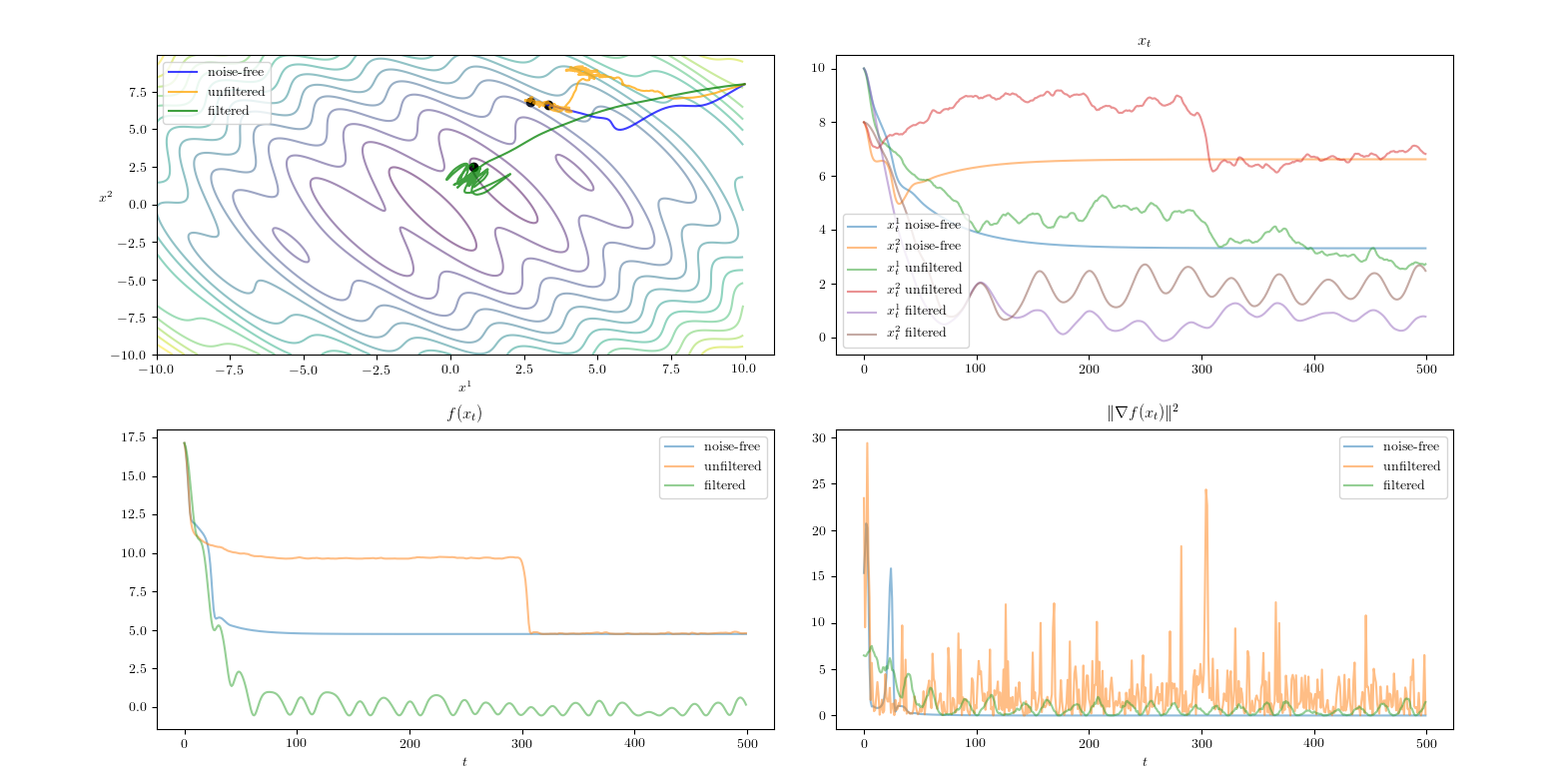
Refer to caption
Refer to caption
Figure 5: Additional tests for filtered stochastic minimization from Section 6.1.