DESY 18–053

DO–TH 18/09

TIF-UNIMI-2018-8

Automated Solution of First Order Factorizable

Systems of Differential Equations

in One Variable

J. Ablingera, J. Blümleinb, P. Marquardb, N. Ranab,c and C. Schneidera

a Research Institute for Symbolic Computation (RISC),
Johannes Kepler University, Altenbergerstraße 69, A–4040, Linz, Austria

b Deutsches Elektronen–Synchrotron, DESY,
Platanenallee 6, D–15738 Zeuthen, Germany

c INFN, Sezione di Milano, Via Celoria 16, I–20133 Milano, Italy

Abstract

We present an algorithm which allows to solve analytically linear systems of differential equations which factorize to first order. The solution is given in terms of iterated integrals over an alphabet where its structure is implied by the coefficient matrix of the differential equations. These systems appear in a large variety of higher order calculations in perturbative Quantum Field Theories. We apply this method to calculate the master integrals of the three–loop massive form factors for different currents, as an illustration, and present the results for the vector form factors in detail. Here the solution space emerging is given by the cyclotomic harmonic polylogarithms and their associated special constants. No special basis representation of the master integrals is needed. The algorithm can be applied as well to more general cases factorizing at first order, which are based on more general alphabets, iterated integrals and associated constants.

1 Introduction

The fundamental objects in any gauge theory are the scattering amplitudes or correlation functions, as they allow to compute the scattering cross sections for collider experiments at large facilities like the Large Hadron Collider (LHC) at CERN. Computations of such objects are mostly using the diagrammatic approach. Especially, in the case of perturbative Quantum Chromodynamics (QCD), one calculates these objects by obtaining all Feynman diagrams at each order in the expansion coefficient, the strong coupling constant αssubscript𝛼𝑠\alpha_{s}. Decades of dedicated work have made it possible to partially automate this procedure, from generating Feynman diagrams to the momentum-integral structure. The main remaining step consists in the computation of the integrals over loop momenta and to perform the associated Feynman parameter integrals.

Through the reduction of the whole problem by integration-by-parts (IBP) techniques [1, 2, 3, 4, 5, 6, 7, 8] one obtains master integrals (MIs). One method to solve these integrals is the method of differential equations [9, 10, 11, 12]. Differentiating with respect to a parameter in the system one obtains coupled systems of ordinary differential equations of master integrals in the uni-variate case, with which we deal with in the following.111For a recent survey on the calculation methods for multi-loop integrals, see Ref. [13]. In the case where these systems factorize at first order, the complete solution can be constructed algorithmically. This has been done before in Ref. [12] mapping to systems of difference equations, which also factorize to first order. The solution has then been performed using difference ring and field technologies [14, 15, 16, 17, 18, 19, 20, 21, 22, 23, 24, 25, 26], implemented in the package Sigma [27, 28].

In the present paper, we present an algorithm operating on uni-variate systems of differential equations, which are factorizing at first order, directly. In the case where the factorization of the system leads to higher order sub-systems, elliptic and even more involved structures will appear, cf. e.g. [29, 30, 31, 32, 33, 34, 35, 36, 37]. Here still iterative solutions can be found. However, the corresponding integrals contain also letters, which are given by non-iterative integrals and therefore these solutions are given by iterative non-iterative integrals [38].

The solution in the first-order factorizing case is given by iterative integrals over a certain alphabet 𝔄={f1(x),fm(x)}𝔄subscript𝑓1𝑥subscript𝑓𝑚𝑥{\mathfrak{A}}=\{f_{1}(x),\dots f_{m}(x)\} together with special constants. We will present the algorithm for solving these systems, which does not require a special choice of a basis for the MIs, like the case in [11].

As an illustration, we employ this method of integration for computing the set of MIs which contribute to both the color–planar and complete light quark non–singlet three-loop contributions to the heavy-quark form factors for different currents, namely the vector, axial-vector, scalar and pseudo-scalar currents. The massive form factors for vector and axial-vector currents play an important role in the forward-backward asymmetry of bottom or top quark pair production at electron-positron and hadron colliders. The scalar and pseudo-scalar ones contribute to the decay of a Higgs boson to a pair of heavy quarks. They are also of importance to scrutinize the properties of the top quark [39, 40] during the high luminosity phase of the LHC [41] and experimental precision studies at future high energy e+esuperscript𝑒superscript𝑒e^{+}e^{-} colliders [42]. The perturbative QCD contributions to these massive form factors at two loops were first computed in [43, 44, 45, 46]. Later an independent computation was performed in [47] for the vector form factors, additionally including 𝒪(ε)𝒪𝜀{\mathcal{O}}(\varepsilon) terms in the dimensional parameter ε=(4D)/2𝜀4𝐷2\varepsilon=(4-D)/2. Recently, the two-loop contributions up to 𝒪(ε2)𝒪superscript𝜀2{\mathcal{O}}(\varepsilon^{2}) for all the massive form factors were obtained in [48]. At three-loop level, the color–planar contributions to the vector form factors have been computed in [50, 49] and the complete light quark contributions in [51]. Using the method described in this paper, we have obtained both the color–planar and complete light quark contributions to the three-loop form factors for the other three currents, namely axial-vector, scalar and pseudo-scalar currents in [52]. In a parallel and independent computation in [53] the same results have been obtained. The asymptotic behaviour of the heavy quark form factors has been studied in [54, 55] recently, see also Refs. [47]. The large β0subscript𝛽0\beta_{0} limit for massive form factors has been considered in [56] and in [57], where the three-loop scalar and pseudo-scalar form factors were computed in the static limit.

The paper is organized as follows. In Section 2 we describe the algorithm to solve first-order factorizing single-variate differential equation systems and present an illustrative example. In Section 3 we consider the massive three-loop vector form factors in an arbitrary basis and present the corresponding analytic results in Section 4. In Section 5 a numerical representation for the cyclotomic harmonic polylogarithms (HPLs) up to weight w = 6 is given, to allow the numerical evaluation of the massive three-loop form factors. Section 6 contains the conclusions. The complete expressions for the vector form factors, which are very large, are given in ancillary files together with the code CPOLY.f for the cyclotomic harmonic polylogarithms and other material, attached to this paper.

2 Description of the method

We consider n𝑛n master integrals (MIs) =(I1,,In)subscript𝐼1subscript𝐼𝑛{\cal I}=(I_{1},\ldots,I_{n}) which belong to the same topology and are functions of the dimensional parameter d=(42ε)𝑑42𝜀d=(4-2\varepsilon) and the variable x𝑥x

s=q2m2=(1x)2x.𝑠superscript𝑞2superscript𝑚2superscript1𝑥2𝑥s=\frac{q^{2}}{m^{2}}=-\frac{(1-x)^{2}}{x}. (1)

Here q2superscript𝑞2q^{2} denotes the virtuality of the current and m𝑚m is the heavy quark mass. One obtains an n×n𝑛𝑛n\times n system of coupled linear differential equations by taking the derivative for x𝑥x of each of the MIs followed by the IBP reduction,

ddx=+.𝑑𝑑𝑥\frac{d}{dx}{\cal I}={\cal M\leavevmode\nobreak\ I+R}. (2)

Here the n×n𝑛𝑛n\times n matrix {\cal M} consists of entries from the rational function field 𝕂(d,x)𝕂𝑑𝑥\mathbb{K}(d,x) (or equivalently from 𝕂(ε,x)𝕂𝜀𝑥\mathbb{K}(\varepsilon,x)) where 𝕂𝕂\mathbb{K} is a field of characteristic 00; in the examples below the entries are even from (d,x)𝑑𝑥\mathbb{Q}(d,x) (or equivalently from (ε,x)𝜀𝑥\mathbb{Q}(\varepsilon,x)). Furthermore, the inhomogeneous part =(1,,n)subscript1subscript𝑛{\cal R}=({\cal R}_{1},\dots,{\cal R}_{n}) is composed by simpler master integrals whose evaluations are immediate or can be carried out by other methods, like symbolic summation and integration; see [12] for details and references therein. In simpler situations {\cal R} turns out to be just the 00-vector. For more involved applications we will assume that each entry isubscript𝑖{\cal R}_{i} is expanded into a Laurent series222In the following f(k)superscript𝑓𝑘f^{(k)} does not denote the k𝑘kth derivative of f𝑓f. in ε𝜀\varepsilon

i=j=kεji(j)subscript𝑖superscriptsubscript𝑗𝑘superscript𝜀𝑗superscriptsubscript𝑖𝑗{\cal R}_{i}=\sum_{j=-k}^{\infty}\varepsilon^{j}{\cal R}_{i}^{(j)}

up to a certain order in terms of special functions. More precisely, we assume that the first coefficients i(j)superscriptsubscript𝑖𝑗{\cal R}_{i}^{(j)} are given as polynomial expressions with coefficients from 𝕂𝕂\mathbb{K} in terms hyperexponential functions and iterative integrals over such functions; for a detailed definition see below. Furthermore, we assume that the unknown integrals isubscript𝑖{\cal I}_{i} can be expanded in an ε𝜀\varepsilon-expansion

i=j=kεji(j).subscript𝑖superscriptsubscript𝑗𝑘superscript𝜀𝑗superscriptsubscript𝑖𝑗{\cal I}_{i}=\sum_{j=-k}^{\infty}\varepsilon^{j}{\cal I}_{i}^{(j)}. (3)

This applies to the case that {\cal M} has no poles in ε𝜀\varepsilon. If this is not the case, according index-shifts have to be performed. Here it may happen that part of the equations which have to be solved, are no differential equations but are algebraic. Given such a coupled system, we seek for the first coefficients i(j)superscriptsubscript𝑖𝑗{\cal I}_{i}^{(j)} in the form of polynomial expressions in terms of hyperexponential functions and iterative integrals over such functions.

Definition. A function f(x)𝑓𝑥f(x) is called hyperexponential if ddxf(x)f(x)=r(x)𝑑𝑑𝑥𝑓𝑥𝑓𝑥𝑟𝑥\frac{\frac{d}{dx}f(x)}{f(x)}=r(x) is a rational function in 𝕂(x)𝕂𝑥\mathbb{K}(x). Such a function may be given in the form

f(x)=elx𝑑yr(y)𝑓𝑥superscript𝑒superscriptsubscript𝑙𝑥differential-d𝑦𝑟𝑦f(x)=e^{\int_{l}^{x}\!\!dy\,r(y)}

for some properly chosen l𝕂𝑙𝕂l\in\mathbb{K}. An iterative integral over hyperexponential functions is an integral of the form

l0x𝑑x1f1(x1)l1x1𝑑x2f2(x2)lλ1xλ1𝑑xλfλ(xλ)superscriptsubscriptsubscript𝑙0𝑥differential-dsubscript𝑥1subscript𝑓1subscript𝑥1superscriptsubscriptsubscript𝑙1subscript𝑥1differential-dsubscript𝑥2subscript𝑓2subscript𝑥2superscriptsubscriptsubscript𝑙𝜆1subscript𝑥𝜆1differential-dsubscript𝑥𝜆subscript𝑓𝜆subscript𝑥𝜆\int_{l_{0}}^{x}\!\!\!dx_{1}\,f_{1}(x_{1})\int_{l_{1}}^{x_{1}}\!\!\!dx_{2}\,f_{2}(x_{2})\dots\int_{l_{\lambda-1}}^{x_{\lambda-1}}\!\!\!dx_{\lambda}\,f_{\lambda}(x_{\lambda}) (4)

where f1(x),,fλ(x)subscript𝑓1𝑥subscript𝑓𝜆𝑥f_{1}(x),\dots,f_{\lambda}(x) are hyperexponential functions and the lower bounds l0,,lλ1𝕂subscript𝑙0subscript𝑙𝜆1𝕂l_{0},\dots,l_{\lambda-1}\in\mathbb{K} are appropriately chosen.

The class of hyperexponential functions covers functions of the form q(x)μ𝑞superscript𝑥𝜇q(x)^{\mu} where q(x)𝕂(x)𝑞𝑥𝕂𝑥q(x)\in\mathbb{K}(x) and μ𝕂𝜇𝕂\mu\in\mathbb{K}. Note that in all our calculations that arose so far, we only dealt with the special case μ𝜇\mu\in\mathbb{Q}. In the following we will use the property that f(x)g(x)𝑓𝑥𝑔𝑥f(x)\,g(x), 1f(x)1𝑓𝑥\frac{1}{f(x)} with f0𝑓0f\neq 0 and ddxf(x)𝑑𝑑𝑥𝑓𝑥\frac{d}{dx}f(x) are hyperexponential functions provided that f(x)𝑓𝑥f(x) and g(x)𝑔𝑥g(x) are hyperexponential functions. In addition, ddx𝑑𝑑𝑥\frac{d}{dx} acting on the iterative integral (4) simply removes the outermost integral. As a consequence, applying the derivative to a polynomial expression in terms of hyperexponential functions and iterative integrals over such functions will lead again to a polynomial expression in terms of such functions. Furthermore, the multiplication of two iterative integrals over hyperexponential functions can be written as a linear combination of iterative integrals over hyperexponential functions due to its shuffle algebra [58]. Consequently also a polynomial expression in terms of hyperexponential functions and iterative integrals over hyperexponential functions can be always written as a linear combination of the form h1(x)I1(x)+hλ(x)Iλ(x)subscript1𝑥subscript𝐼1𝑥subscript𝜆𝑥subscript𝐼𝜆𝑥h_{1}(x)I_{1}(x)+\dots h_{\lambda}(x)I_{\lambda}(x) where the Ii(x)subscript𝐼𝑖𝑥I_{i}(x) are iterative integrals over hyperexponential functions and the hi(x)subscript𝑖𝑥h_{i}(x) are hyperexponential functions.

A general assumption of our method will be that the degree of uncoupling will be of first order. More precisely, we will apply internally Zürcher’s algorithm [59, 61, 60] implemented in the package OreSys [62] in order to decompose the system into one scalar linear differential equation (sometimes also several such equations) determining all unknown functions. In the case that the scalar equations (evaluated at ε=0𝜀0\varepsilon=0) are first-order factorizable, we proceed.

In general, the dimension n𝑛n of the system (2) is rather high (e.g., n=100𝑛100n=100). In this matter we note that the MIs can be distinguished sector-wise. A sector is defined by a set of maximum number of non-vanishing propagators in a single Feynman graph. Correspondingly, the absence of some propagators defines sub-sectors. The differential equation of a MI hence only contains integrals from the same sector or its sub-sectors. Thus, organizing the integrals in a way such that integrals with a minimum number of propagators are kept at the end of the list, provides an upper-block-triangular form of {\cal M}, i.e. the diagonal elements of {\cal M} are square matrices of not only rank one but higher. Each such square matrix represents a completely coupled set of integrals and we call them sub-systems of {\cal M}. The advantage of arranging the system in this way is that now we can solve the system in a bottom-up approach, i.e. we first solve for the last set of coupled integrals in the list which depend on themselves only (plus inhomogeneous parts from {\cal R} that are already expanded in terms of special functions), and then solve the second last set of coupled integrals, which depends on themselves and the last integrals and thus going up in the list.

We will now elaborate the different steps of our proposed algorithm. Similar ideas have been utilized already in Refs. [63, 12, 64, 65] in order to find solutions in terms of iterative sums over hypergeometric products.

1. Let us consider m𝑚m integrals ~=(I~1,,I~m)~subscript~𝐼1subscript~𝐼𝑚{\cal\tilde{I}}=(\tilde{I}_{1},\ldots,\tilde{I}_{m}) which constitute a coupled sub-system,

ddx~=~~+~,𝑑𝑑𝑥~~~~\frac{d}{dx}{\cal\tilde{I}}={\cal\tilde{M}\leavevmode\nobreak\ \tilde{I}+\tilde{R}}, (5)

where the non-diagonal elements of ~~{\cal\tilde{M}} are mostly non-zero and are rational functions from 𝕂(d,x)𝕂𝑑𝑥\mathbb{K}(d,x), or equivalently from 𝕂(ε,x)𝕂𝜀𝑥\mathbb{K}(\varepsilon,x). In particular, we may assume that ~~{\cal\tilde{M}} is an invertible matrix; if not, one can derive an alternative system by simple row operations with this property (the new system consists of less unknown integrals and the redundant integrals, that are removed from the system, can be expressed trivially by the integrals that arise in the new system). The inhomogeneity ~~{\cal\tilde{R}} is formed by contributions from integrals belonging to sub-sectors and the components of {\cal R}. By construction we succeeded already in calculating the first coefficients of the ε𝜀\varepsilon-expansions of these integrals in terms of iterative integrals over hyperexponential functions. Consequently, plugging these results into {\cal R} yields the ε𝜀\varepsilon-expansions

~i=j=kεj~i(j)subscript~𝑖superscriptsubscript𝑗𝑘superscript𝜀𝑗superscriptsubscript~𝑖𝑗{\cal\tilde{R}}_{i}=\sum_{j=-k}^{\infty}\varepsilon^{j}{\cal\tilde{R}}_{i}^{(j)}

for 1im1𝑖𝑚1\leq i\leq m where the first coefficients ~i(j)superscriptsubscript~𝑖𝑗{\cal\tilde{R}}_{i}^{(j)} are given explicitly in terms of iterative integrals over hyperexponential functions.
Now we exploit the fact that for a certain topology and kinematics, the order k𝑘k of highest pole of an integral in ~~{\cal\tilde{I}} is well-defined, as e.g. the integrals arising in three-loop massive form factors can have at most a pole of 1/ε31superscript𝜀31/\varepsilon^{3}. Hence, one has the following Laurent expansions

~i=j=kεj~i(j).subscript~𝑖superscriptsubscript𝑗𝑘superscript𝜀𝑗superscriptsubscript~𝑖𝑗{\cal\tilde{I}}_{i}=\sum_{j=-k}^{\infty}\varepsilon^{j}{\cal\tilde{I}}_{i}^{(j)}. (6)

In order to determine the first coefficients ~isubscript~𝑖{\cal\tilde{I}}_{i} in terms of iterative integrals, we proceed as follows. We plug in (3) with undetermined coefficients ~isubscript~𝑖{\cal\tilde{I}}_{i} into (5), perform the series expansion in ε𝜀\varepsilon and consider the coefficient of εksuperscript𝜀𝑘\varepsilon^{k} :

ddx~(k)=~M(0)~I(k)+(~M(1)~I(k1)+~M(2)~I(k2)++~M(k+l)~I(l))+~(k),𝑑𝑑𝑥superscript~𝑘~absentsuperscript𝑀0~absentsuperscript𝐼𝑘~absentsuperscript𝑀1~absentsuperscript𝐼𝑘1~absentsuperscript𝑀2~absentsuperscript𝐼𝑘2~absentsuperscript𝑀𝑘𝑙~absentsuperscript𝐼𝑙superscript~𝑘\frac{d}{dx}{\cal\tilde{I}}^{(k)}={\tilde{\cal}M^{(0)}\leavevmode\nobreak\ \tilde{\cal}I^{(k)}+\Big{(}\tilde{\cal}M^{(1)}\leavevmode\nobreak\ \tilde{\cal}I^{(k-1)}+\tilde{\cal}M^{(2)}\leavevmode\nobreak\ \tilde{\cal}I^{(k-2)}+\cdots+\tilde{\cal}M^{(k+l)}\leavevmode\nobreak\ \tilde{\cal}I^{(-l)}\Big{)}+\tilde{\cal R}^{(k)}}, (7)

for k=l,l+1,etc.𝑘𝑙𝑙1𝑒𝑡𝑐k=-l,-l+1,etc.

2. At each order in the ε𝜀\varepsilon-expansion we have now functions of a single variable x𝑥x only. Solving order by order, one obtains ~~{\cal\tilde{I}} as a Laurent series expansion in ε𝜀\varepsilon. To accomplish that we start with the coefficient of the leading pole εlsuperscript𝜀𝑙\varepsilon^{-l}. The corresponding sub-system is

ddx~(l)=~M(0)~I(l)+~(l).𝑑𝑑𝑥superscript~𝑙~absentsuperscript𝑀0~absentsuperscript𝐼𝑙superscript~𝑙\frac{d}{dx}{\cal\tilde{I}}^{(-l)}={\tilde{\cal}M^{(0)}\leavevmode\nobreak\ \tilde{\cal}I^{(-l)}+\tilde{\cal R}^{(-l)}}\,. (8)

To solve Eq. (8), a natural first step is to reduce this m×m𝑚𝑚m\times m system to a higher order differential equation for a single integral. We will refer to this procedure as ‘uncoupling’ from now on. By using the package OreSys one obtains

k=0mpk(x)dkdxk~1(l)(x)=r(x).superscriptsubscript𝑘0𝑚subscript𝑝𝑘𝑥superscript𝑑𝑘𝑑superscript𝑥𝑘subscriptsuperscript~𝑙1𝑥𝑟𝑥\sum_{k=0}^{m}p_{k}(x)\frac{d^{k}}{dx^{k}}{\cal\tilde{I}}^{(-l)}_{1}(x)=r(x). (9)

Here pl(x)subscript𝑝𝑙𝑥p_{l}(x) are rational functions in 𝕂(x)𝕂𝑥\mathbb{K}(x) and

r(x)=i=0λj=1mri,j(x)didxi~j(l)(x)𝑟𝑥superscriptsubscript𝑖0𝜆superscriptsubscript𝑗1𝑚subscript𝑟𝑖𝑗𝑥superscript𝑑𝑖𝑑superscript𝑥𝑖subscriptsuperscript~𝑙𝑗𝑥r(x)=\sum_{i=0}^{\lambda}\sum_{j=1}^{m}r_{i,j}(x)\,\frac{d^{i}}{dx^{i}}{\cal\tilde{R}}^{(-l)}_{j}(x) (10)

for some integer λ𝜆\lambda. Since the differentiation of iterative integrals over hyperexponential functions yields again iterative integrals over hyperexponential functions, the inhomogeneous part r(x)𝑟𝑥r(x) can be given explicitly in terms of iterative integrals over hyperexponential functions. Besides this scalar differential equation, the package OreSys provides in addition the solutions ~k(l)(x)|k=2mevaluated-atsubscriptsuperscript~𝑙𝑘𝑥𝑘2𝑚\left.{\cal\tilde{I}}^{(-l)}_{k}(x)\right|_{k=2}^{m} in terms of linear combinations of ~1(l)(x)subscriptsuperscript~𝑙1𝑥{\cal\tilde{I}}^{(-l)}_{1}(x) and its derivatives:

~k(l)(x)=i=0m1ak,i(x)didxi~k(l)(x)+ρk(x)subscriptsuperscript~𝑙𝑘𝑥superscriptsubscript𝑖0𝑚1subscript𝑎𝑘𝑖𝑥superscript𝑑𝑖𝑑superscript𝑥𝑖subscriptsuperscript~𝑙𝑘𝑥subscript𝜌𝑘𝑥{\cal\tilde{I}}^{(-l)}_{k}(x)=\sum_{i=0}^{m-1}a_{k,i}(x)\,\frac{d^{i}}{dx^{i}}{\cal\tilde{I}}^{(-l)}_{k}(x)+\rho_{k}(x) (11)

with ak,i𝕂(x)subscript𝑎𝑘𝑖𝕂𝑥a_{k,i}\in\mathbb{K}(x). Like the r(x)𝑟𝑥r(x) in (10) the ρk(x)subscript𝜌𝑘𝑥\rho_{k}(x) can be given in such a form. Consequently, also the ρk(x)subscript𝜌𝑘𝑥\rho_{k}(x) can be expressed explicitly in terms of iterative integrals over hyperexponential functions. In other words, if one succeeds in solving the linear differential equations (9) and obtains the solution for ~1(l)(x)subscriptsuperscript~𝑙1𝑥{\cal\tilde{I}}^{(-l)}_{1}(x) in terms of iterative integrals over hyperexponential functions, one can plug this closed form into (11) and can extract such an integral representation of the remaining functions ~k(l)(x)|k=2mevaluated-atsubscriptsuperscript~𝑙𝑘𝑥𝑘2𝑚\left.{\cal\tilde{I}}^{(-l)}_{k}(x)\right|_{k=2}^{m}. Concerning the uncoupling we remark that it is not advised using the classical cyclic vector algorithm to achieve the uncoupling, since generally this method provides uncoupled equations with large coefficients. Moreover, it is beneficial that Zürcher’s algorithm may find several linear differential equations for several of the unknown functions: they have usually smaller orders than the cyclic vector algorithm (which always finds only one differential equation). The solving tools are now applied to each of the found equations. For simplicity we assume in the following that only one scalar differential equation for ~1(l)(x)subscriptsuperscript~𝑙1𝑥{\cal\tilde{I}}^{(-l)}_{1}(x) is produced.

3. From Eq. (7) it is evident that the homogeneous solutions are always the same for any order in ε𝜀\varepsilon. The inhomogeneous solutions are different, however, by action of the inhomogeneities. We first consider the homogeneous solutions of Eq. (9). First we check if the differential equation can be factorized into first-order factors of the form

(ddxp^1(x))(ddxp^2(x))(ddxp^m(x))y1(x)=0,𝑑𝑑𝑥subscript^𝑝1𝑥𝑑𝑑𝑥subscript^𝑝2𝑥𝑑𝑑𝑥subscript^𝑝𝑚𝑥subscript𝑦1𝑥0\left(\frac{d}{dx}-\hat{p}_{1}(x)\right)\left(\frac{d}{dx}-\hat{p}_{2}(x)\right){\dots}\left(\frac{d}{dx}-\hat{p}_{m}(x)\right)y_{1}(x)=0, (12)

with p^ksubscript^𝑝𝑘\hat{p}_{k} being rational functions in 𝕂(x)𝕂𝑥\mathbb{K}(x) by using algorithms from [66, 67, 68]; for more details see [69, Chapter 4]. If this is possible, we proceed as follows. Define for 1km1𝑘𝑚1\leq k\leq m the hyperexponential functions

hk(x)=elkx𝑑yp^k(y)subscript𝑘𝑥superscript𝑒superscriptsubscriptsubscriptsuperscript𝑙𝑘𝑥differential-d𝑦subscript^𝑝𝑘𝑦h_{k}(x)=e^{\int_{l^{\prime}_{k}}^{x}\!\!dy\,\hat{p}_{k}(y)} (13)

for some appropriate lower bounds lk𝕂subscriptsuperscript𝑙𝑘𝕂l^{\prime}_{k}\in\mathbb{K}, that are solutions of the k𝑘kth first-order factor, i.e.,

(ddxp^k(x))hk(x)=0ddxhk(x)hk(x)=p^k(x).formulae-sequence𝑑𝑑𝑥subscript^𝑝𝑘𝑥subscript𝑘𝑥0𝑑𝑑𝑥subscript𝑘𝑥subscript𝑘𝑥subscript^𝑝𝑘𝑥\left(\frac{d}{dx}-\hat{p}_{k}(x)\right)h_{k}(x)=0\quad\Longleftrightarrow\quad\frac{\frac{d}{dx}h_{k}(x)}{h_{k}(x)}=\hat{p}_{k}(x). (14)

Finally, one can read off from the factorization (12) the m𝑚m solutions

y1(x)=h1(x),y2(x)=h1(x)l0x𝑑x1h2(x1)h1(x1),ym(x)=h1(x)l0x𝑑x1h2(x1)h1(x1)l1x1𝑑x2h3(x2)h2(x2)lm2xm2𝑑xm1hm(xm1)hm1(xm1),formulae-sequencesubscript𝑦1𝑥subscript1𝑥formulae-sequencesubscript𝑦2𝑥subscript1𝑥superscriptsubscriptsubscript𝑙0𝑥differential-dsubscript𝑥1subscript2subscript𝑥1subscript1subscript𝑥1subscript𝑦𝑚𝑥subscript1𝑥superscriptsubscriptsubscript𝑙0𝑥differential-dsubscript𝑥1subscript2subscript𝑥1subscript1subscript𝑥1superscriptsubscriptsubscript𝑙1subscript𝑥1differential-dsubscript𝑥2subscript3subscript𝑥2subscript2subscript𝑥2superscriptsubscriptsubscript𝑙𝑚2subscript𝑥𝑚2differential-dsubscript𝑥𝑚1subscript𝑚subscript𝑥𝑚1subscript𝑚1subscript𝑥𝑚1\begin{split}y_{1}(x)=&h_{1}(x),\\ y_{2}(x)=&h_{1}(x)\int_{l_{0}}^{x}\!\!\!dx_{1}\,\frac{h_{2}(x_{1})}{h_{1}(x_{1})},\\ \vdots&\\ y_{m}(x)=&h_{1}(x)\int_{l_{0}}^{x}\!\!\!dx_{1}\,\frac{h_{2}(x_{1})}{h_{1}(x_{1})}\int_{l_{1}}^{x_{1}}\!\!\!dx_{2}\,\frac{h_{3}(x_{2})}{h_{2}(x_{2})}\dots\int_{l_{m-2}}^{x_{m-2}}\!\!\!dx_{m-1}\,\frac{h_{m}(x_{m-1})}{h_{m-1}(x_{m-1})},\end{split} (15)

where the lower bounds l0,,lm2subscript𝑙0subscript𝑙𝑚2l_{0},\dots,l_{m-2} are chosen accordingly. These solutions, also called d’Alembertian solutions [70], form iterative integrals over hyperexponential functions hk(x)hk1(x)subscript𝑘𝑥subscript𝑘1𝑥\frac{h_{k}(x)}{h_{k-1}(x)}. Since they are linearly independent over 𝕂𝕂\mathbb{K}, see [70, Thm. 5],

{C1y1(x)++Cmym(x)C1,,Cm𝕂}conditional-setsubscript𝐶1subscript𝑦1𝑥subscript𝐶𝑚subscript𝑦𝑚𝑥subscript𝐶1subscript𝐶𝑚𝕂\{C_{1}\,y_{1}(x)+\dots+C_{m}\,y_{m}(x)\,\mid\,C_{1},\dots,C_{m}\in\mathbb{K}\}

yield the full solution space of the homogeneous recurrence (12). In the calculations presented below the hyperexponential functions hk(x)subscript𝑘𝑥h_{k}(x) can be simplified all to rational functions in 𝕂𝕂\mathbb{K}. Even more is true after further simplifications: The integrands can be decomposed into the form

hk(x)hk1(x)=qk+lqk,lϕl(x),qk,qk,l𝕂formulae-sequencesubscript𝑘𝑥subscript𝑘1𝑥subscript𝑞𝑘subscript𝑙subscript𝑞𝑘𝑙subscriptitalic-ϕ𝑙𝑥subscript𝑞𝑘subscript𝑞𝑘𝑙𝕂\frac{h_{k}(x)}{h_{k-1}(x)}=q_{k}+\sum_{l}q_{k,l}\phi_{l}(x),\leavevmode\nobreak\ \leavevmode\nobreak\ \leavevmode\nobreak\ \leavevmode\nobreak\ q_{k},q_{k,l}\in\mathbb{K} (16)

by partial fractioning with ϕl(x)=αl(x)βl(x)elsubscriptitalic-ϕ𝑙𝑥subscript𝛼𝑙𝑥subscript𝛽𝑙superscript𝑥subscript𝑒𝑙\phi_{l}(x)=\frac{\alpha_{l}(x)}{\beta_{l}(x)^{e_{l}}} where the βl(x)subscript𝛽𝑙𝑥\beta_{l}(x) are irreducible polynomials in 𝕂[x]𝕂delimited-[]𝑥\mathbb{K}[x] and αl(x)subscript𝛼𝑙𝑥\alpha_{l}(x) are polynomials in 𝕂[x]𝕂delimited-[]𝑥\mathbb{K}[x] with deg(αl(x))<deg(βl(x))degreesubscript𝛼𝑙𝑥degreesubscript𝛽𝑙𝑥\deg(\alpha_{l}(x))<\deg(\beta_{l}(x)) and el\{0}subscript𝑒𝑙\0e_{l}\in\mathbb{N}\backslash\{0\}.

Let us consider a typical example. Usually the functions p^k(x)subscript^𝑝𝑘𝑥\hat{p}_{k}(x) in Eq. (12) are rational functions, which factor into the letters fl(x)subscript𝑓𝑙𝑥f_{l}(x) of an alphabet 𝔄superscript𝔄{\mathfrak{A}}^{\prime}. If these letters are the ones of the Kummer-Poincaré type [71] the ratios hm/hm1subscript𝑚subscript𝑚1h_{m}/h_{m-1} in Eqs. (15) are again Kummer-Poincaré letters after partial fractioning. This representation holds as well for cyclotomic harmonic polylogarithms, since these have complex representations by Kummer-Poincaré letters.

By linearity one can now apply the integration sign to each of the summands in (16) and eliminate algebraic relations among the arising integrals utilizing their shuffle relations; these ideas have been elaborated in detail for the sum case [58, 72]. In particular, the multiplicity elsubscript𝑒𝑙e_{l} can be reduced upon noting

𝑑x1xk=1(k1)1xk1,𝑑x1(1±x)k=1(k1)1(1±x)k1.formulae-sequencedifferential-d𝑥1superscript𝑥𝑘1𝑘11superscript𝑥𝑘1differential-d𝑥1superscriptplus-or-minus1𝑥𝑘minus-or-plus1𝑘11superscriptplus-or-minus1𝑥𝑘1\int dx\frac{1}{x^{k}}=\frac{-1}{(k-1)}\frac{1}{x^{k-1}},\leavevmode\nobreak\ \leavevmode\nobreak\ \int dx\frac{1}{(1\pm x)^{k}}=\frac{\mp 1}{(k-1)}\frac{1}{(1\pm x)^{k-1}}. (17)

Likewise, the cyclotomic letters integrate to structures like

𝑑x1(1x+x2)3differential-d𝑥1superscript1𝑥superscript𝑥23\displaystyle\int dx\frac{1}{(1-x+x^{2})^{3}} =\displaystyle= 2x16(1x+x2)2+2x13(1x+x2)+23𝑑x11x+x22𝑥16superscript1𝑥superscript𝑥222𝑥131𝑥superscript𝑥223differential-d𝑥11𝑥superscript𝑥2\displaystyle\frac{2x-1}{6(1-x+x^{2})^{2}}+\frac{2x-1}{3(1-x+x^{2})}+\frac{2}{3}\int dx\,\frac{1}{1-x+x^{2}} (18)
𝑑xx(1+x+x2)2differential-d𝑥𝑥superscript1𝑥superscript𝑥22\displaystyle\int dx\frac{x}{(1+x+x^{2})^{2}} =\displaystyle= x+23(1+x+x2)13𝑑x11+x+x2,etc.𝑥231𝑥superscript𝑥213differential-d𝑥11𝑥superscript𝑥2etc\displaystyle-\frac{x+2}{3(1+x+x^{2})}-\frac{1}{3}\int dx\,\frac{1}{1+x+x^{2}},\leavevmode\nobreak\ \leavevmode\nobreak\ {\rm etc.} (19)

In the course of these simplifications also products of these functions and corresponding harmonic polylogarithms arise that can be joined using shuffle relations [58]. In addition to the cyclotomic harmonic polylogarithms also their corresponding values at x=1𝑥1x=1 contribute through partial integration. In the case of the harmonic polylogarithms these are the multiple zeta values (MZVs) [73]. In the cyclotomic case they are given by the cyclotomic constants [74, 75, 77, 76]. In [78] relations beyond those known from [74, 75, 77, 76] already have been conjectured using PSLQ [79]. More generally, this tactic can be applied in combination with the Almkvist–Zeilberger algorithm [80] if in addition hyperexponential functions arise that cannot be handled by the simplifications described above. In summary, a homogeneous linear differential equation stored in the variable de in terms of the unknown function f(x)𝑓𝑥f(x) can be solved in terms of d’Alembertian solutions by executing the HarmonicSums command

SolveDE[de,f[x],x].SolveDE[de,f[x],x]\texttt{SolveDE[de,f[x],x]}.

In particular, if a factorization of the form (12) exists for the given differential operator, it will be computed and the full set of solutions (15) will be produced where all the simplifications described above are applied.
In all our applications so far, the homogeneous solutions yi(x),i=1,,mformulae-sequencesubscript𝑦𝑖𝑥𝑖1𝑚y_{i}(x),i=1,\ldots,m could be expressed in terms of iterative integrals

b,a(x)=0x𝑑yfb(y)b,a(y),=1,formulae-sequencesubscript𝑏𝑎𝑥superscriptsubscript0𝑥differential-d𝑦subscript𝑓𝑏𝑦subscript𝑏𝑎𝑦subscript1{\cal H}_{b,\vec{a}}(x)=\int_{0}^{x}dyf_{b}(y){\cal H}_{b,\vec{a}}(y),\leavevmode\nobreak\ \leavevmode\nobreak\ \leavevmode\nobreak\ {\cal H}_{\emptyset}=1, (20)

where fb(y)𝔄subscript𝑓𝑏𝑦𝔄f_{b}(y)\in\mathfrak{A} are rational functions (or roots of rational functions) taken from a finite alphabet 𝔄𝔄\mathfrak{A}. For instance, for the massive three-loop form factor discussed below, the alphabet can be chosen by

𝔄={1x,11x,11+x,11+x2,x1+x2,11+x+x2,x1+x+x2,11x+x2,x1x+x2},𝔄1𝑥11𝑥11𝑥11superscript𝑥2𝑥1superscript𝑥211𝑥superscript𝑥2𝑥1𝑥superscript𝑥211𝑥superscript𝑥2𝑥1𝑥superscript𝑥2\mathfrak{A}=\left\{\tfrac{1}{x},\leavevmode\nobreak\ \tfrac{1}{1-x},\leavevmode\nobreak\ \tfrac{1}{1+x},\leavevmode\nobreak\ \tfrac{1}{1+x^{2}},\leavevmode\nobreak\ \tfrac{x}{1+x^{2}},\leavevmode\nobreak\ \tfrac{1}{1+x+x^{2}},\leavevmode\nobreak\ \tfrac{x}{1+x+x^{2}},\leavevmode\nobreak\ \tfrac{1}{1-x+x^{2}},\leavevmode\nobreak\ \tfrac{x}{1-x+x^{2}}\right\}, (21)

where fb(x)subscript𝑓𝑏𝑥f_{b}(x) corresponds to the b𝑏bth entry. Summarizing, in our concrete application below the arising d’Alembertian solutions (15) will be simplified to expressions in terms of the class of harmonic polylogarithms [81] and the cyclotomic harmonic polylogarithms [77].

4. The solution of the inhomogeneous differential equation (9) can be given explicitly by the following iterative integral [70]

g(x)=h1(x)l0x𝑑x1h2(x1)h1(x1)l1x1𝑑x2h3(x2)h2(x2)lm2xm2𝑑xm1hm(xm1)hm1(xm1)lm1xm1𝑑xmr(xm)hm(xm).𝑔𝑥subscript1𝑥superscriptsubscriptsubscript𝑙0𝑥differential-dsubscript𝑥1subscript2subscript𝑥1subscript1subscript𝑥1superscriptsubscriptsubscript𝑙1subscript𝑥1differential-dsubscript𝑥2subscript3subscript𝑥2subscript2subscript𝑥2superscriptsubscriptsubscript𝑙𝑚2subscript𝑥𝑚2differential-dsubscript𝑥𝑚1subscript𝑚subscript𝑥𝑚1subscript𝑚1subscript𝑥𝑚1superscriptsubscriptsubscript𝑙𝑚1subscript𝑥𝑚1differential-dsubscript𝑥𝑚𝑟subscript𝑥𝑚subscript𝑚subscript𝑥𝑚g(x)=h_{1}(x)\int_{l_{0}}^{x}\!\!\!dx_{1}\,\frac{h_{2}(x_{1})}{h_{1}(x_{1})}\int_{l_{1}}^{x_{1}}\!\!\!dx_{2}\,\frac{h_{3}(x_{2})}{h_{2}(x_{2})}\dots\int_{l_{m-2}}^{x_{m-2}}\!\!\!dx_{m-1}\,\frac{h_{m}(x_{m-1})}{h_{m-1}(x_{m-1})}\int_{l_{m-1}}^{x_{m-1}}\!\!\!dx_{m}\,\frac{r(x_{m})}{h_{m}(x_{m})}. (22)

Consequently,

~1(l)(x)=g(x)+C1y1(x)++Cmym(x)subscriptsuperscript~𝑙1𝑥𝑔𝑥subscript𝐶1subscript𝑦1𝑥subscript𝐶𝑚subscript𝑦𝑚𝑥{\cal\tilde{I}}^{(-l)}_{1}(x)=g(x)+C_{1}\,y_{1}(x)+\dots+C_{m}\,y_{m}(x) (23)

where the constants Cisubscript𝐶𝑖C_{i} are implied by (physical) boundary conditions and they are usually determined by separate calculations. Since the inhomogeneous part r(x)𝑟𝑥r(x) can be given in terms of iterative integrals over hyperexponential functions, also g(x)𝑔𝑥g(x) and thus ~1(l)(x)subscriptsuperscript~𝑙1𝑥{\cal\tilde{I}}^{(-l)}_{1}(x) can be expressed in terms of iterative integral over hyperexponential functions. Furthermore, using our simplification tools from above, these integrals can be simplified further. E.g., within all our calculations we end up at alphabets of the form (21) or variants involving also rooted letters.
We want to emphasize an alternative approach to find a particular solution g(x)𝑔𝑥g(x) of (9). If

W(x)=|y1ymddxy1(1)ddxymdm1dxm1y1dm1dxm1ym|𝑊𝑥subscript𝑦1subscript𝑦𝑚𝑑𝑑𝑥superscriptsubscript𝑦11𝑑𝑑𝑥subscript𝑦𝑚missing-subexpressionsuperscript𝑑𝑚1𝑑superscript𝑥𝑚1subscript𝑦1missing-subexpressionsuperscript𝑑𝑚1𝑑superscript𝑥𝑚1subscript𝑦𝑚W(x)=\left|\begin{array}[]{ccc}y_{1}&\ldots&y_{m}\\ \frac{d}{dx}y_{1}^{(1)}&\ldots&\frac{d}{dx}y_{m}\\ \vdots&&\vdots\\ \frac{d^{m-1}}{dx^{m-1}}y_{1}&&\frac{d^{m-1}}{dx^{m-1}}y_{m}\\ \end{array}\right| (24)

is the Wronskian of the linear differential equation (9) and

Wi(x)=(1)i+m|y1yi1yi+1ymddxy1ddxyi1ddxyi+1ddxymdm2dxm2y1dm2dxm2yi1dm2dxm2yi+1dm2dxm2ym|,subscript𝑊𝑖𝑥superscript1𝑖𝑚subscript𝑦1subscript𝑦𝑖1subscript𝑦𝑖1subscript𝑦𝑚𝑑𝑑𝑥subscript𝑦1𝑑𝑑𝑥subscript𝑦𝑖1𝑑𝑑𝑥subscript𝑦𝑖1𝑑𝑑𝑥subscript𝑦𝑚missing-subexpressionmissing-subexpressionsuperscript𝑑𝑚2𝑑superscript𝑥𝑚2subscript𝑦1superscript𝑑𝑚2𝑑superscript𝑥𝑚2subscript𝑦𝑖1superscript𝑑𝑚2𝑑superscript𝑥𝑚2subscript𝑦𝑖1superscript𝑑𝑚2𝑑superscript𝑥𝑚2subscript𝑦𝑚W_{i}(x)=(-1)^{i+m}\left|\begin{array}[]{cccccc}y_{1}&\ldots&y_{i-1}&y_{i+1}&\ldots&y_{m}\\ \frac{d}{dx}y_{1}&\ldots&\frac{d}{dx}y_{i-1}&\frac{d}{dx}y_{i+1}&\ldots&\frac{d}{dx}y_{m}\\ \vdots&&\vdots&\vdots&&\vdots\\ \frac{d^{m-2}}{dx^{m-2}}y_{1}&\ldots&\frac{d^{m-2}}{dx^{m-2}}y_{i-1}&\frac{d^{m-2}}{dx^{m-2}}y_{i+1}&\ldots&\frac{d^{m-2}}{dx^{m-2}}y_{m}\\ \end{array}\right|, (25)

then

g(x)=i=1myi(x)lx𝑑x~r(x~)Wi(x~)W(x~)𝑔𝑥superscriptsubscript𝑖1𝑚subscript𝑦𝑖𝑥superscriptsubscript𝑙𝑥differential-d~𝑥𝑟~𝑥subscript𝑊𝑖~𝑥𝑊~𝑥g(x)=\sum_{i=1}^{m}y_{i}(x)\int_{l}^{x}d\tilde{x}\frac{r(\tilde{x})W_{i}(\tilde{x})}{W(\tilde{x})} (26)

for some appropriately chosen l𝕂𝑙𝕂l\in\mathbb{K} yields another particular solution. Note that by (a mild generalization) of Abel’s theorem we have that W(x)𝑊𝑥W(x) itself can be written as a hyperexponential function

W(x)=celx𝑑ypm1(y)pm(y)𝑊𝑥𝑐superscript𝑒superscriptsubscript𝑙𝑥differential-d𝑦subscript𝑝𝑚1𝑦subscript𝑝𝑚𝑦W(x)=c\,e^{-\int_{l}^{x}\!\!dy\frac{p_{m-1}(y)}{p_{m}(y)}}

for some constant c𝕂𝑐𝕂c\in\mathbb{K} and an appropriately chosen lower bound l𝕂𝑙𝕂l\in\mathbb{K}; the polynomials pm(x),pm1(x)𝕂[x]subscript𝑝𝑚𝑥subscript𝑝𝑚1𝑥𝕂delimited-[]𝑥p_{m}(x),p_{m-1}(x)\in\mathbb{K}[x] come from the linear differential equation (9). Furthermore, the Wi(x)subscript𝑊𝑖𝑥W_{i}(x) are given by polynomial expressions in terms of the homogeneous solutions yi(x)subscript𝑦𝑖𝑥y_{i}(x). As a consequence r(x~)Wi(x~)W(x~)𝑟~𝑥subscript𝑊𝑖~𝑥𝑊~𝑥\frac{r(\tilde{x})W_{i}(\tilde{x})}{W(\tilde{x})} in (26) forms a polynomial expression in terms of hyperexponential functions and iterative integrals over such functions. In particular, g(x)𝑔𝑥g(x) yields such a representation.
The following extra bonus often makes the formula (26) superior to (4): By reusing the simplified homogeneous solutions y1(x),,ym(x)subscript𝑦1𝑥subscript𝑦𝑚𝑥y_{1}(x),\dots,y_{m}(x) for (26), it is much easier to obtain a simplification of (26) than of (4) in terms of iterative integrals of the form (20) with alphabets like (21).

5. Now we plug this representation of ~1(l)(x)subscriptsuperscript~𝑙1𝑥{\cal\tilde{I}}^{(-l)}_{1}(x) in terms of iterative integrals into (11) for k=2,,m𝑘2𝑚k=2,\dots,m. Since the derivation of iterative integrals over hyperexponential functions yields again iterative integrals over hyperexponential functions, all entries in the vector ~1(l)(x)subscriptsuperscript~𝑙1𝑥{\cal\tilde{I}}^{(-l)}_{1}(x) can be given within the class of iterative integrals over hyperexponential functions.

6. Finally, we plug this representation of ~(l)(x)superscript~𝑙𝑥{\cal\tilde{I}}^{(-l)}(x) in terms of iterative integrals into (7) for k=l+1𝑘𝑙1k=-l+1 and obtain a new system of the form (8) for the εl+1superscript𝜀𝑙1\varepsilon^{-l+1}-coefficient ~(l+1)=(~1(l+1)(x),,~m(l+1)(x))superscript~𝑙1superscriptsubscript~1𝑙1𝑥superscriptsubscript~𝑚𝑙1𝑥{\cal\tilde{I}}^{(-l+1)}=({\cal\tilde{I}}_{1}^{(-l+1)}(x),\dots,{\cal\tilde{I}}_{m}^{(-l+1)}(x)). Thus we repeat the game for εl+1superscript𝜀𝑙1\varepsilon^{-l+1} and the remaining coefficients in (3) by induction/recursion. We note once more that the formula (23) remains the same, except that in (26) the function r(x)𝑟𝑥r(x) changes. As a consequence one can again reuse the already simplified homogeneous solutions y1(x),,ym(x)subscript𝑦1𝑥subscript𝑦𝑚𝑥y_{1}(x),\dots,y_{m}(x) and just needs to simplify g(x)𝑔𝑥g(x) in (26) with the updated function r(x)𝑟𝑥r(x).

Let us illustrate the above algorithm by an example, which concerns the solution of a sub-system in the calculation of the three loop massive form factors in the color planar limit.

Example.
We consider the following system of differential equations for the integrals {J1,J2,J3}subscript𝐽1subscript𝐽2subscript𝐽3\{J_{1},J_{2},J_{3}\}\in{\cal I}:

ddx(J1J2J3)=[c11c12c13c21c22c23c31c32c33](J1J2J3)+(R1(ϵ,x)R2(ϵ,x)R3(ϵ,x)),𝑑𝑑𝑥subscript𝐽1subscript𝐽2subscript𝐽3delimited-[]subscript𝑐11subscript𝑐12subscript𝑐13subscript𝑐21subscript𝑐22subscript𝑐23subscript𝑐31subscript𝑐32subscript𝑐33subscript𝐽1subscript𝐽2subscript𝐽3subscript𝑅1italic-ϵ𝑥subscript𝑅2italic-ϵ𝑥subscript𝑅3italic-ϵ𝑥\displaystyle\begin{split}\frac{d}{dx}\left(\begin{array}[]{l}J_{1}\\ J_{2}\\ J_{3}\end{array}\right)&=\left[\begin{array}[]{ccc}c_{11}&c_{12}&c_{13}\\ c_{21}&c_{22}&c_{23}\\ c_{31}&c_{32}&c_{33}\\ \end{array}\right]\left(\begin{array}[]{l}J_{1}\\ J_{2}\\ J_{3}\end{array}\right)+\left(\begin{array}[]{l}R_{1}(\epsilon,x)\\ R_{2}(\epsilon,x)\\ R_{3}(\epsilon,x)\end{array}\right),\end{split} (27)

where cijsubscript𝑐𝑖𝑗c_{ij}’s are rational functions in d𝑑d, resp. ε𝜀\varepsilon, and x𝑥x as given by

c11subscript𝑐11\displaystyle c_{11} =(7+6x+7x22d(1+x+x2))x(1x2),c12=(4+d)(10+3d)2(3+d)2(1x2),formulae-sequenceabsent76𝑥7superscript𝑥22𝑑1𝑥superscript𝑥2𝑥1superscript𝑥2subscript𝑐124𝑑103𝑑2superscript3𝑑21superscript𝑥2\displaystyle=\frac{\big{(}7+6x+7x^{2}-2d\big{(}1+x+x^{2}\big{)}\big{)}}{x(1-x^{2})}\,,c_{12}=\frac{(-4+d)(-10+3d)}{2(-3+d)^{2}(1-x^{2})}\,,
c13subscript𝑐13\displaystyle c_{13} =(d2(15+8x+15x2)+8(20+9x+20x2)2d(49+24x+49x2))4(3+d)2x(1x2),absentsuperscript𝑑2158𝑥15superscript𝑥28209𝑥20superscript𝑥22𝑑4924𝑥49superscript𝑥24superscript3𝑑2𝑥1superscript𝑥2\displaystyle=\frac{\big{(}d^{2}\big{(}15+8x+15x^{2}\big{)}+8\big{(}20+9x+20x^{2}\big{)}-2d\big{(}49+24x+49x^{2}\big{)}\big{)}}{4(-3+d)^{2}x(1-x^{2})}\,,
c21subscript𝑐21\displaystyle c_{21} =(3+d)2(d(3+x)(1+3x)2(518x+5x2))(10+3d)x(1x2),c22=(7+2d)(1+x2)x(1x2),formulae-sequenceabsentsuperscript3𝑑2𝑑3𝑥13𝑥2518𝑥5superscript𝑥2103𝑑𝑥1superscript𝑥2subscript𝑐2272𝑑1superscript𝑥2𝑥1superscript𝑥2\displaystyle=\frac{(-3+d)^{2}\big{(}d(-3+x)(-1+3x)-2\big{(}5-18x+5x^{2}\big{)}\big{)}}{(-10+3d)x(1-x^{2})}\,,c_{22}=\frac{(-7+2d)\big{(}1+x^{2}\big{)}}{x(1-x^{2})}\,,
c23subscript𝑐23\displaystyle c_{23} =(30+188x30x2+d2(3+16x3x2)+d(19110x+19x2))(10+3d)x(1x2),absent30188𝑥30superscript𝑥2superscript𝑑2316𝑥3superscript𝑥2𝑑19110𝑥19superscript𝑥2103𝑑𝑥1superscript𝑥2\displaystyle=\frac{\big{(}-30+188x-30x^{2}+d^{2}\big{(}-3+16x-3x^{2}\big{)}+d\big{(}19-110x+19x^{2}\big{)}\big{)}}{(-10+3d)x(1-x^{2})}\,,
c31subscript𝑐31\displaystyle c_{31} =(3+d)2(1+x)x(1x),c32=0,c33=2(3+d)(1+x+x2)x(1x2).formulae-sequenceabsentsuperscript3𝑑21𝑥𝑥1𝑥formulae-sequencesubscript𝑐320subscript𝑐3323𝑑1𝑥superscript𝑥2𝑥1superscript𝑥2\displaystyle=-\frac{(-3+d)^{2}(1+x)}{x(1-x)}\,,c_{32}=0\,,c_{33}=\frac{2(-3+d)\big{(}1+x+x^{2}\big{)}}{x(1-x^{2})}\,. (28)

The functions Ri(ε,x)subscript𝑅𝑖𝜀𝑥R_{i}(\varepsilon,x) contain the inhomogeneous contributions from sub-sectors. They can be expanded into a Laurent series expansion in ε𝜀\varepsilon up to the required order and read

R1(ε,x)subscript𝑅1𝜀𝑥\displaystyle R_{1}(\varepsilon,x) =13(1x2)1ε31x6x(1+x)1ε2[2+11x+2x23x(1x2)9ζ22(1x2)]1εabsent131superscript𝑥21superscript𝜀31𝑥6𝑥1𝑥1superscript𝜀2delimited-[]211𝑥2superscript𝑥23𝑥1superscript𝑥29subscript𝜁221superscript𝑥21𝜀\displaystyle=\frac{1}{3(1-x^{2})}\frac{1}{\varepsilon^{3}}-\frac{1-x}{6x(1+x)}\frac{1}{\varepsilon^{2}}-\left[\frac{2+11x+2x^{2}}{3x(1-x^{2})}-\frac{9\zeta_{2}}{2(1-x^{2})}\right]\frac{1}{\varepsilon}
14x+188x24x3+x46x2(1x2)(134x+x2)ζ24x(1x2)+31ζ33(1x2)+2xH0+1x2x(1+x)H0214𝑥188superscript𝑥24superscript𝑥3superscript𝑥46superscript𝑥21superscript𝑥2134𝑥superscript𝑥2subscript𝜁24𝑥1superscript𝑥231subscript𝜁331superscript𝑥22𝑥subscriptH01𝑥2𝑥1𝑥superscriptsubscriptH02\displaystyle-\frac{1-4x+188x^{2}-4x^{3}+x^{4}}{6x^{2}(1-x^{2})}-\frac{(1-34x+x^{2})\zeta_{2}}{4x(1-x^{2})}+\frac{31\zeta_{3}}{3(1-x^{2})}+\frac{2}{x}{\rm H}_{0}+\frac{1-x}{2x(1+x)}{\rm H}_{0}^{2}
23(1x2)H038(12H02H1H0H0,1+H0,0,1)1x2+O(ε)231superscript𝑥2superscriptsubscriptH03812superscriptsubscriptH02subscriptH1subscriptH0subscriptH01subscriptH0011superscript𝑥2𝑂𝜀\displaystyle-\frac{2}{3(1-x^{2})}{\rm H}_{0}^{3}-\frac{8\left(\tfrac{1}{2}{\rm H}_{0}^{2}{\rm H}_{1}-{\rm H}_{0}{\rm H}_{0,1}+{\rm H}_{0,0,1}\right)}{1-x^{2}}+O(\varepsilon) (29)
R2(ε,x)subscript𝑅2𝜀𝑥\displaystyle R_{2}(\varepsilon,x) =1+x6x(1x)1ε3+3+2x+3x26x(1x2)1ε2+[115x+16x215x3+x46x2(1x2)+(1+x)ζ24x(1x)+H0x\displaystyle=\frac{1+x}{6x(1-x)}\frac{1}{\varepsilon^{3}}+\frac{3+2x+3x^{2}}{6x(1-x^{2})}\frac{1}{\varepsilon^{2}}+\Biggl{[}-\frac{1-15x+16x^{2}-15x^{3}+x^{4}}{6x^{2}(1-x^{2})}+\frac{(1+x)\zeta_{2}}{4x(1-x)}+\frac{{\rm H}_{0}}{x}
(1+4x+x2)2x(1x2)H02]1ε(1x)(959x+9x2)6x2(1+x)(12x7x2)ζ24x(1x2)\displaystyle-\frac{(1+4x+x^{2})}{2x(1-x^{2})}{\rm H}_{0}^{2}\Biggr{]}\frac{1}{\varepsilon}-\frac{(1-x)(9-59x+9x^{2})}{6x^{2}(1+x)}-\frac{(1-2x-7x^{2})\zeta_{2}}{4x(1-x^{2})}
+(25+110x+25x2)ζ36x(1x2)+(114x+x22x2+(1+4x+x2)ζ2x(1x2))H025110𝑥25superscript𝑥2subscript𝜁36𝑥1superscript𝑥2114𝑥superscript𝑥22superscript𝑥214𝑥superscript𝑥2subscript𝜁2𝑥1superscript𝑥2subscriptH0\displaystyle+\frac{(25+110x+25x^{2})\zeta_{3}}{6x(1-x^{2})}+\left(-\frac{1-14x+x^{2}}{2x^{2}}+\frac{(1+4x+x^{2})\zeta_{2}}{x(1-x^{2})}\right){\rm H}_{0}
+13x6x2x(1x2)H025+22x+5x26x(1x2)H0310xH1,0+4x(H0H1H0,1)+10+40x+10x2x(1x2)13𝑥6superscript𝑥2𝑥1superscript𝑥2superscriptsubscriptH02522𝑥5superscript𝑥26𝑥1superscript𝑥2superscriptsubscriptH0310𝑥subscriptH104𝑥subscriptH0subscriptH1subscriptH011040𝑥10superscript𝑥2𝑥1superscript𝑥2\displaystyle+\frac{1-3x-6x^{2}}{x(1-x^{2})}{\rm H}_{0}^{2}-\frac{5+22x+5x^{2}}{6x(1-x^{2})}{\rm H}_{0}^{3}-\frac{10}{x}{\rm H}_{-1,0}+\frac{4}{x}\left({\rm H}_{0}{\rm H}_{1}-{\rm H}_{0,1}\right)+\frac{10+40x+10x^{2}}{x(1-x^{2})}
×(H0H1,02H1,0,0)4(1+4x+x2)x(1x2)(H0H0,12H0,0,1)+4(1+3x+x2x(1x2)(12H02H1\displaystyle\times\left({\rm H}_{0}{\rm H}_{-1,0}-2{\rm H}_{-1,0,0}\right)-\frac{4(1+4x+x^{2})}{x(1-x^{2})}\left({\rm H}_{0}{\rm H}_{0,1}-2{\rm H}_{0,0,1}\right)+\frac{4(1+3x+x^{2}}{x(1-x^{2})}\Bigl{(}\frac{1}{2}{\rm H}_{0}^{2}{\rm H}_{1}
H0H0,1+H0,0,1)+O(ε)\displaystyle-{\rm H}_{0}{\rm H}_{0,1}+{\rm H}_{0,0,1}\Bigr{)}+O(\varepsilon) (30)
R3(ε,x)subscript𝑅3𝜀𝑥\displaystyle R_{3}(\varepsilon,x) =13(1x2)1ε3+13(1x2)1ε2+[1+2x8x2+2x3+x46x2(1x2)+9ζ22(1x2)]1εabsent131superscript𝑥21superscript𝜀3131superscript𝑥21superscript𝜀2delimited-[]12𝑥8superscript𝑥22superscript𝑥3superscript𝑥46superscript𝑥21superscript𝑥29subscript𝜁221superscript𝑥21𝜀\displaystyle=\frac{1}{3(1-x^{2})}\frac{1}{\varepsilon^{3}}+\frac{1}{3(1-x^{2})}\frac{1}{\varepsilon^{2}}+\left[\frac{1+2x-8x^{2}+2x^{3}+x^{4}}{6x^{2}(1-x^{2})}+\frac{9\zeta_{2}}{2(1-x^{2})}\right]\frac{1}{\varepsilon}
+9+18x76x2+18x3+9x46x2(1x2)+9ζ22(1x2)+31ζ33(1x2)+1+4x+x22x2H011x2H02918𝑥76superscript𝑥218superscript𝑥39superscript𝑥46superscript𝑥21superscript𝑥29subscript𝜁221superscript𝑥231subscript𝜁331superscript𝑥214𝑥superscript𝑥22superscript𝑥2subscriptH011superscript𝑥2superscriptsubscriptH02\displaystyle+\frac{9+18x-76x^{2}+18x^{3}+9x^{4}}{6x^{2}(1-x^{2})}+\frac{9\zeta_{2}}{2(1-x^{2})}+\frac{31\zeta_{3}}{3(1-x^{2})}+\frac{1+4x+x^{2}}{2x^{2}}{\rm H}_{0}-\frac{1}{1-x^{2}}{\rm H}_{0}^{2}
23(1x2)H0381x2[12H02H1H0H0,1+H0,0,1]+O(ε).231superscript𝑥2superscriptsubscriptH0381superscript𝑥2delimited-[]12superscriptsubscriptH02subscriptH1subscriptH0subscriptH01subscriptH001𝑂𝜀\displaystyle-\frac{2}{3(1-x^{2})}{\rm H}_{0}^{3}-\frac{8}{1-x^{2}}\left[\frac{1}{2}{\rm H}_{0}^{2}{\rm H}_{1}-{\rm H}_{0}{\rm H}_{0,1}+{\rm H}_{0,0,1}\right]+O(\varepsilon). (31)

Here we use the convention Ha(x)HasubscriptH𝑎𝑥subscriptH𝑎{\rm H}_{\vec{a}}(x)\equiv{\rm H}_{\vec{a}} and ζl=k=11/kl,l,l2formulae-sequencesubscript𝜁𝑙superscriptsubscript𝑘11superscript𝑘𝑙formulae-sequence𝑙𝑙2\zeta_{l}=\sum_{k=1}^{\infty}1/k^{l},\leavevmode\nobreak\ \leavevmode\nobreak\ l\in\mathbb{N},l\geq 2 denote the values of Riemann’s ζ𝜁\zeta-function. The harmonic polylogarithms [81] are defined by

Hb,a(x)=0x𝑑yfb(y)Ha(y),H=1,b,ai{1,0,1},formulae-sequencesubscriptH𝑏𝑎𝑥superscriptsubscript0𝑥differential-d𝑦subscript𝑓𝑏𝑦subscriptH𝑎𝑦formulae-sequencesubscriptH1𝑏subscript𝑎𝑖101{\rm H}_{b,\vec{a}}(x)=\int_{0}^{x}dyf_{b}(y){\rm H}_{\vec{a}}(y),\leavevmode\nobreak\ \leavevmode\nobreak\ {\rm H}_{\emptyset}=1,\leavevmode\nobreak\ \leavevmode\nobreak\ b,a_{i}\in\{-1,0,1\}, (32)

and the letters fcsubscript𝑓𝑐f_{c} are

f0(x)=1x,f1(x)=11x,f1(x)=11+x.formulae-sequencesubscript𝑓0𝑥1𝑥formulae-sequencesubscript𝑓1𝑥11𝑥subscript𝑓1𝑥11𝑥f_{0}(x)=\frac{1}{x},\leavevmode\nobreak\ \leavevmode\nobreak\ \leavevmode\nobreak\ \leavevmode\nobreak\ f_{1}(x)=\frac{1}{1-x},\leavevmode\nobreak\ \leavevmode\nobreak\ \leavevmode\nobreak\ \leavevmode\nobreak\ f_{-1}(x)=\frac{1}{1+x}. (33)

The HPLs are dual, by the Mellin transform, to the harmonic sums [82, 83].

The solutions Jisubscript𝐽𝑖J_{i} are calculated in terms of the following expansion in ε𝜀\varepsilon

Ji(x,ε)=1ε3Ji(3)+1ε2Ji(2)+1εJi(1)+Ji(0)+O(ε).subscript𝐽𝑖𝑥𝜀1superscript𝜀3superscriptsubscript𝐽𝑖31superscript𝜀2superscriptsubscript𝐽𝑖21𝜀superscriptsubscript𝐽𝑖1superscriptsubscript𝐽𝑖0𝑂𝜀J_{i}(x,\varepsilon)=\frac{1}{\varepsilon^{3}}J_{i}^{(-3)}+\frac{1}{\varepsilon^{2}}J_{i}^{(-2)}+\frac{1}{\varepsilon}J_{i}^{(-1)}+J_{i}^{(0)}+O(\varepsilon). (34)

First, one obtains the determining equation for the leading pole O(1/ε3)𝑂1superscript𝜀3O(1/\varepsilon^{3}):

ddx(J13J23J33)=[1x+21x011+x2x31x1x+21+x11+x1x11x1x21+x1x+21x011+x2x31x](J13J23J33)+(R13(x)R23(x)R33(x)).𝑑𝑑𝑥superscriptsubscript𝐽13superscriptsubscript𝐽23superscriptsubscript𝐽33delimited-[]1𝑥21𝑥011𝑥2𝑥31𝑥1𝑥21𝑥11𝑥1𝑥11𝑥1𝑥21𝑥1𝑥21𝑥011𝑥2𝑥31𝑥superscriptsubscript𝐽13superscriptsubscript𝐽23superscriptsubscript𝐽33superscriptsubscript𝑅13𝑥superscriptsubscript𝑅23𝑥superscriptsubscript𝑅33𝑥\displaystyle\begin{split}\frac{d}{dx}\left(\begin{array}[]{l}J_{1}^{-3}\\ J_{2}^{-3}\\ J_{3}^{-3}\end{array}\right)&=-\left[\begin{array}[]{ccc}\frac{1}{x}+\frac{2}{1-x}&0&\frac{1}{1+x}-\frac{2}{x}-\frac{3}{1-x}\\ -\frac{1}{x}+\frac{2}{1+x}&\frac{1}{1+x}-\frac{1}{x}-\frac{1}{1-x}&\frac{1}{x}-\frac{2}{1+x}\\ \frac{1}{x}+\frac{2}{1-x}&0&\frac{1}{1+x}-\frac{2}{x}-\frac{3}{1-x}\\ \end{array}\right]\left(\begin{array}[]{l}J_{1}^{-3}\\ J_{2}^{-3}\\ J_{3}^{-3}\end{array}\right)+\left(\begin{array}[]{l}R_{1}^{-3}(x)\\ R_{2}^{-3}(x)\\ R_{3}^{-3}(x)\end{array}\right).\end{split} (35)

Using the incomplete Zürcher algorithm, one of four algorithms implemented in OreSys, we obtain for Eq. (35) two uncoupled differential equations, one of order two for J3(x)subscript𝐽3𝑥J_{3}(x) and another of first order for J2(x)subscript𝐽2𝑥J_{2}(x). J1(x)subscript𝐽1𝑥J_{1}(x) can directly be obtained from the solution for J3(x)subscript𝐽3𝑥J_{3}(x).

The second order differential equation for J3(x)subscript𝐽3𝑥J_{3}(x)

[d2dx221xddx+(2x21+x2(1+x)2)]J33(x)delimited-[]superscript𝑑2𝑑superscript𝑥221𝑥𝑑𝑑𝑥2𝑥21𝑥2superscript1𝑥2superscriptsubscript𝐽33𝑥\displaystyle\bigg{[}\frac{d^{2}}{dx^{2}}-\frac{2}{1-x}\frac{d}{dx}+\Big{(}\frac{2}{x}-\frac{2}{1+x}-\frac{2}{(1+x)^{2}}\Big{)}\bigg{]}J_{3}^{-3}(x) =r33(x)absentsuperscriptsubscript𝑟33𝑥\displaystyle=r_{3}^{-3}(x) (36)

with the inhomogeneous part

r33(x)=13x13(1+x)13(1+x)2superscriptsubscript𝑟33𝑥13𝑥131𝑥13superscript1𝑥2\displaystyle r_{3}^{-3}(x)=\frac{1}{3x}-\frac{1}{3(1+x)}-\frac{1}{3(1+x)^{2}} (37)

needs to be solved first. The differential operator in Eq. (36) can be written in factorized form

D𝐷\displaystyle D =\displaystyle= (ddxp1(x))(ddxp2(x)),𝑑𝑑𝑥subscript𝑝1𝑥𝑑𝑑𝑥subscript𝑝2𝑥\displaystyle\left(\frac{d}{dx}-p_{1}(x)\right)\circ\left(\frac{d}{dx}-p_{2}(x)\right), (38)
p1(x)subscript𝑝1𝑥\displaystyle p_{1}(x) =\displaystyle= 11x1x+11+x,11𝑥1𝑥11𝑥\displaystyle\frac{1}{1-x}-\frac{1}{x}+\frac{1}{1+x}, (39)
p2(x)subscript𝑝2𝑥\displaystyle p_{2}(x) =\displaystyle= 11x+1x11+x.11𝑥1𝑥11𝑥\displaystyle\frac{1}{1-x}+\frac{1}{x}-\frac{1}{1+x}. (40)

In this case the rational functions p^i(x)subscript^𝑝𝑖𝑥\hat{p}_{i}(x) are linear combinations of the letters spanning the HPLs. One now uses the method of the variation of the constants to obtain the solutions for the differential equation. The homogeneous solutions y1(x),y2(x)subscript𝑦1𝑥subscript𝑦2𝑥y_{1}(x),y_{2}(x) are given by

y1(x)=x1x2,y2(x)=12x1x2H0,formulae-sequencesubscript𝑦1𝑥𝑥1superscript𝑥2subscript𝑦2𝑥12𝑥1superscript𝑥2subscriptH0y_{1}(x)=\frac{x}{1-x^{2}}\,,\quad y_{2}(x)=1-\frac{2x}{1-x^{2}}{\rm H}_{0}\,, (41)

and we obtain the solution

J33(x)=y1(x)[C1𝑑xr33(x)y2(x)W(y1,y2)]+y2(x)[C2+𝑑xr33(x)y1(x)W(y1,y2)].superscriptsubscript𝐽33𝑥subscript𝑦1𝑥delimited-[]subscript𝐶1differential-d𝑥superscriptsubscript𝑟33𝑥subscript𝑦2𝑥𝑊subscript𝑦1subscript𝑦2subscript𝑦2𝑥delimited-[]subscript𝐶2differential-d𝑥superscriptsubscript𝑟33𝑥subscript𝑦1𝑥𝑊subscript𝑦1subscript𝑦2\displaystyle J_{3}^{-3}(x)=y_{1}(x)\bigg{[}C_{1}-\int dx\frac{r_{3}^{-3}(x)y_{2}(x)}{W(y_{1},y_{2})}\bigg{]}+y_{2}(x)\bigg{[}C_{2}+\int dx\frac{r_{3}^{-3}(x)y_{1}(x)}{W(y_{1},y_{2})}\bigg{]}\,. (42)

where the constants Cisubscript𝐶𝑖C_{i} can be determined from the physical boundary conditions and are known from a separate calculation. With the Wronskian W𝑊W given by

W(y1,y2)=1(1x)2,𝑊subscript𝑦1subscript𝑦21superscript1𝑥2W(y_{1},y_{2})=-\frac{1}{(1-x)^{2}}\,, (43)

the integrals in (42) are easily evaluated

𝑑xr33(x)y2(x)W(y1,y2)differential-d𝑥superscriptsubscript𝑟33𝑥subscript𝑦2𝑥𝑊subscript𝑦1subscript𝑦2\displaystyle\int dx\frac{r_{3}^{-3}(x)y_{2}(x)}{W(y_{1},y_{2})} =\displaystyle= 23(1+x)1+x23(1+x)2H0,231𝑥1superscript𝑥23superscript1𝑥2subscriptH0\displaystyle-\frac{2}{3(1+x)}-\frac{1+x^{2}}{3(1+x)^{2}}{\rm H}_{0}, (44)
𝑑xr33(x)y1(x)W(y1,y2)differential-d𝑥superscriptsubscript𝑟33𝑥subscript𝑦1𝑥𝑊subscript𝑦1subscript𝑦2\displaystyle\int dx\frac{r_{3}^{-3}(x)y_{1}(x)}{W(y_{1},y_{2})} =\displaystyle= x3(1+x)2.𝑥3superscript1𝑥2\displaystyle-\frac{x}{3(1+x)^{2}}\,. (45)

For the remaining constants we find

C1=13,C2=16,formulae-sequencesubscript𝐶113subscript𝐶216C_{1}=-\frac{1}{3}\,,\leavevmode\nobreak\ \leavevmode\nobreak\ \leavevmode\nobreak\ C_{2}=\frac{1}{6}\,, (46)

and thus

J33(x)superscriptsubscript𝐽33𝑥\displaystyle J_{3}^{-3}(x) =16.absent16\displaystyle=\hskip 8.53581pt\frac{1}{6}\,. (47)

The solution for integral J13(x)superscriptsubscript𝐽13𝑥J_{1}^{-3}(x) can directly be obtained from this result

J13(x)=x3(1+x)2+2(1+x+x2)(1+x)2J33(x)(1x)xx+1ddxJ33(x)=13.superscriptsubscript𝐽13𝑥𝑥3superscript1𝑥221𝑥superscript𝑥2superscript1𝑥2superscriptsubscript𝐽33𝑥1𝑥𝑥𝑥1𝑑𝑑𝑥superscriptsubscript𝐽33𝑥13\displaystyle J_{1}^{-3}(x)=\frac{x}{3(1+x)^{2}}+\frac{2\left(1+x+x^{2}\right)}{(1+x)^{2}}J_{3}^{-3}(x)-\frac{(1-x)x}{x+1}\frac{d}{dx}J_{3}^{-3}(x)=\frac{1}{3}\,. (48)

With these results at hand we can obtain the first order differential equation for J23(x)superscriptsubscript𝐽23𝑥J_{2}^{-3}(x)

[ddx(11x+1x11+x)]J23(x)delimited-[]𝑑𝑑𝑥11𝑥1𝑥11𝑥superscriptsubscript𝐽23𝑥\displaystyle\bigg{[}\frac{d}{dx}-\Big{(}\frac{1}{1-x}+\frac{1}{x}-\frac{1}{1+x}\Big{)}\bigg{]}J_{2}^{-3}(x) =r23(x),absentsuperscriptsubscript𝑟23𝑥\displaystyle=r_{2}^{-3}(x), (49)

where the inhomogeneous part is given by

r23(x)=13x13(1+x)+13(1x).superscriptsubscript𝑟23𝑥13𝑥131𝑥131𝑥\displaystyle r_{2}^{-3}(x)=\frac{1}{3x}-\frac{1}{3(1+x)}+\frac{1}{3(1-x)}. (50)

The homogenous solution is given by

y3(x)=x1x2subscript𝑦3𝑥𝑥1superscript𝑥2y_{3}(x)=\frac{x}{1-x^{2}}

and thus we can obtain the full solution by evaluating

J23(x)=y3(x)(C3+𝑑xr23(x)y3(x)).superscriptsubscript𝐽23𝑥subscript𝑦3𝑥subscript𝐶3differential-d𝑥superscriptsubscript𝑟23𝑥subscript𝑦3𝑥\displaystyle J_{2}^{-3}(x)=y_{3}(x)\bigg{(}C_{3}+\int dx\frac{r_{2}^{-3}(x)}{y_{3}(x)}\bigg{)}\,. (51)

The integral is easily evaluated

𝑑xr23(x)y3(x)differential-d𝑥superscriptsubscript𝑟23𝑥subscript𝑦3𝑥\displaystyle\int dx\frac{r_{2}^{-3}(x)}{y_{3}(x)} =\displaystyle= 1x23x,1superscript𝑥23𝑥\displaystyle-\frac{1-x^{2}}{3x}\,, (52)

and after fixing the constant of integration

C3=0subscript𝐶30C_{3}=0 (53)

we obtain the final result

J23(x)superscriptsubscript𝐽23𝑥\displaystyle J_{2}^{-3}(x) =13.absent13\displaystyle=-\frac{1}{3}\,. (54)

To summarize, the results obtained so far, the solutions J1(3),J2(3),J3(3)superscriptsubscript𝐽13superscriptsubscript𝐽23superscriptsubscript𝐽33J_{1}^{(-3)},J_{2}^{(-3)},J_{3}^{(-3)} are given by the numbers:

J13(x)superscriptsubscript𝐽13𝑥\displaystyle J_{1}^{-3}(x) =13,absent13\displaystyle=\hskip 8.53581pt\frac{1}{3}, (55)
J23(x)superscriptsubscript𝐽23𝑥\displaystyle J_{2}^{-3}(x) =13,absent13\displaystyle=-\frac{1}{3}, (56)
J33(x)superscriptsubscript𝐽33𝑥\displaystyle J_{3}^{-3}(x) =16.absent16\displaystyle=\hskip 8.53581pt\frac{1}{6}\leavevmode\nobreak\ . (57)

Now, once the sub-system is solved for the highest pole, we consider the next order in ε𝜀\varepsilon. By construction, the homogeneous structure of the sub-system remains the same for any order in ε𝜀\varepsilon and hence the uncoupling procedure. The only change that takes place for different orders in ε𝜀\varepsilon is in the inhomogeneous parts which also constitute the contributions from the already-known previous orders in ε𝜀\varepsilon-expansion. Thus, for higher orders in ε𝜀\varepsilon, the only step is to iterate Eqs. (42) and (51). In this way we obtain the following solutions for the functions J1,J2,J3subscript𝐽1subscript𝐽2subscript𝐽3J_{1},J_{2},J_{3} up to O(ε0)𝑂superscript𝜀0O(\varepsilon^{0}). Here we use the basis for the harmonic polylogarithms defined in [84].

J12(x)superscriptsubscript𝐽12𝑥\displaystyle J_{1}^{-2}(x) =53absent53\displaystyle=\frac{5}{3} (58)
J22(x)superscriptsubscript𝐽22𝑥\displaystyle J_{2}^{-2}(x) =2absent2\displaystyle=-2 (59)
J32(x)superscriptsubscript𝐽32𝑥\displaystyle J_{3}^{-2}(x) =12absent12\displaystyle=\frac{1}{2} (60)
J11(x)superscriptsubscript𝐽11𝑥\displaystyle J_{1}^{-1}(x) =1+22x+x26x+92ζ2absent122𝑥superscript𝑥26𝑥92subscript𝜁2\displaystyle=\frac{1+22x+x^{2}}{6x}+\frac{9}{2}\zeta_{2} (61)
J21(x)superscriptsubscript𝐽21𝑥\displaystyle J_{2}^{-1}(x) =283+12H022x3(1x2)H0352ζ24xζ21x2H0absent28312superscriptsubscriptH022𝑥31superscript𝑥2superscriptsubscriptH0352subscript𝜁24𝑥subscript𝜁21superscript𝑥2subscriptH0\displaystyle=-\frac{28}{3}+\frac{1}{2}{\rm H}_{0}^{2}-\frac{2x}{3(1-x^{2})}{\rm H}_{0}^{3}-\frac{5}{2}\zeta_{2}-\frac{4x\zeta_{2}}{1-x^{2}}{\rm H}_{0} (62)
J31(x)superscriptsubscript𝐽31𝑥\displaystyle J_{3}^{-1}(x) =16+94ζ2absent1694subscript𝜁2\displaystyle=\frac{1}{6}+\frac{9}{4}\zeta_{2} (63)
J1(0)(x)superscriptsubscript𝐽10𝑥\displaystyle J_{1}^{(0)}(x) =1346x+13x26x+1x22xH0+12H02+1+3x23(1x2)H03x4(1x2)H04absent1346𝑥13superscript𝑥26𝑥1superscript𝑥22𝑥subscriptH012superscriptsubscriptH0213superscript𝑥231superscript𝑥2superscriptsubscriptH03𝑥41superscript𝑥2superscriptsubscriptH04\displaystyle=\frac{13-46x+13x^{2}}{6x}+\frac{1-x^{2}}{2x}{\rm H}_{0}+\frac{1}{2}{\rm H}_{0}^{2}+\frac{1+3x^{2}}{3(1-x^{2})}{\rm H}_{0}^{3}-\frac{x}{4(1-x^{2})}{\rm H}_{0}^{4}
+(2H024xH033(1x2))H1+(4H0+2x1x2H02)H0,14H0,0,14x1x2H0,0,0,12superscriptsubscriptH024𝑥superscriptsubscriptH0331superscript𝑥2subscriptH14subscriptH02𝑥1superscript𝑥2superscriptsubscriptH02subscriptH014subscriptH0014𝑥1superscript𝑥2subscriptH0001\displaystyle+\left(-2{\rm H}_{0}^{2}-\frac{4x{\rm H}_{0}^{3}}{3(1-x^{2})}\right){\rm H}_{1}+\left(4{\rm H}_{0}+\frac{2x}{1-x^{2}}{\rm H}_{0}^{2}\right){\rm H}_{0,1}-4{\rm H}_{0,0,1}-\frac{4x}{1-x^{2}}{\rm H}_{0,0,0,1}
+(492+4(1+x2)1x2H02x1x2H028x1x2H0H1+8x1x2H0,1)ζ232xζ225(1x2)+313ζ349241superscript𝑥21superscript𝑥2subscriptH02𝑥1superscript𝑥2superscriptsubscriptH028𝑥1superscript𝑥2subscriptH0subscriptH18𝑥1superscript𝑥2subscriptH01subscript𝜁232𝑥superscriptsubscript𝜁2251superscript𝑥2313subscript𝜁3\displaystyle+\left(\frac{49}{2}+\frac{4\big{(}1+x^{2}\big{)}}{1-x^{2}}{\rm H}_{0}-\frac{2x}{1-x^{2}}{\rm H}_{0}^{2}-\frac{8x}{1-x^{2}}{\rm H}_{0}{\rm H}_{1}+\frac{8x}{1-x^{2}}{\rm H}_{0,1}\right)\zeta_{2}-\frac{32x\zeta_{2}^{2}}{5(1-x^{2})}+\frac{31}{3}\zeta_{3} (64)
J2(0)(x)superscriptsubscript𝐽20𝑥\displaystyle J_{2}^{(0)}(x) =4016x1x2(H0H0,0,13H0,0,0,1)+16x1x2[16(H0H1H0,1)H0213H02H0,1+H0H0,0,1\displaystyle=-40-\frac{16x}{1-x^{2}}\big{(}{\rm H}_{0}{\rm H}_{0,0,1}-3{\rm H}_{0,0,0,1}\big{)}+\frac{16x}{1-x^{2}}\Biggl{[}\frac{1}{6}\big{(}{\rm H}_{0}{\rm H}_{1}-{\rm H}_{0,1}\big{)}{\rm H}_{0}^{2}-\frac{1}{3}{\rm H}_{0}^{2}{\rm H}_{0,1}+{\rm H}_{0}{\rm H}_{0,0,1}
H0,0,0,1]+16x1x2[12H02H0,12H0H0,0,1+3H0,0,0,1]+40x1x2[12H02H1,02H0H1,0,0\displaystyle-{\rm H}_{0,0,0,1}\Biggr{]}+\frac{16x}{1-x^{2}}\Biggl{[}\frac{1}{2}{\rm H}_{0}^{2}{\rm H}_{0,1}-2{\rm H}_{0}{\rm H}_{0,0,1}+3{\rm H}_{0,0,0,1}\Biggr{]}+\frac{40x}{1-x^{2}}\Biggl{[}\frac{1}{2}{\rm H}_{0}^{2}{\rm H}_{-1,0}-2{\rm H}_{0}{\rm H}_{-1,0,0}
+3H1,0,0,0]+4(H0H0,12H0,0,1)10(H0H1,02H1,0,0)2[12H02H1H0H0,1\displaystyle+3{\rm H}_{-1,0,0,0}\Biggr{]}+4\big{(}{\rm H}_{0}{\rm H}_{0,1}-2{\rm H}_{0,0,1}\big{)}-10\big{(}{\rm H}_{0}{\rm H}_{-1,0}-2{\rm H}_{-1,0,0}\big{)}-2\Biggl{[}\frac{1}{2}{\rm H}_{0}^{2}{\rm H}_{1}-{\rm H}_{0}{\rm H}_{0,1}
+H0,0,1][(3+x)ζ21x8xζ31x2]H0+[3+8xζ21x2]H02+2(12x)3(1x)H03x3(1x2)H04\displaystyle+{\rm H}_{0,0,1}\Biggr{]}-\Biggl{[}\frac{(3+x)\zeta_{2}}{1-x}-\frac{8x\zeta_{3}}{1-x^{2}}\Biggr{]}{\rm H}_{0}+\Biggl{[}3+\frac{8x\zeta_{2}}{1-x^{2}}\Biggr{]}{\rm H}_{0}^{2}+\frac{2(1-2x)}{3(1-x)}{\rm H}_{0}^{3}-\frac{x}{3(1-x^{2})}{\rm H}_{0}^{4}
8x1x2H1,0,0,015ζ2+16x1x2(H0H1H0,1)ζ28xζ21x2H1,0+96xζ225(1x2)283ζ38𝑥1superscript𝑥2subscriptH100015subscript𝜁216𝑥1superscript𝑥2subscriptH0subscriptH1subscriptH01subscript𝜁28𝑥subscript𝜁21superscript𝑥2subscriptH1096𝑥superscriptsubscript𝜁2251superscript𝑥2283subscript𝜁3\displaystyle-\frac{8x}{1-x^{2}}{\rm H}_{-1,0,0,0}-15\zeta_{2}+\frac{16x}{1-x^{2}}\big{(}{\rm H}_{0}{\rm H}_{1}-{\rm H}_{0,1}\big{)}\zeta_{2}-\frac{8x\zeta_{2}}{1-x^{2}}{\rm H}_{-1,0}+\frac{96x\zeta_{2}^{2}}{5(1-x^{2})}-\frac{28}{3}\zeta_{3} (65)
J3(0)(x)superscriptsubscript𝐽30𝑥\displaystyle J_{3}^{(0)}(x) =1528x1x2[16(H0H1H0,1)H0213H02H0,1+H0H0,0,1H0,0,0,1]4x1x2[12H02H0,1\displaystyle=-\frac{15}{2}-\frac{8x}{1-x^{2}}\Biggl{[}\frac{1}{6}\big{(}{\rm H}_{0}{\rm H}_{1}-{\rm H}_{0,1}\big{)}{\rm H}_{0}^{2}-\frac{1}{3}{\rm H}_{0}^{2}{\rm H}_{0,1}+{\rm H}_{0}{\rm H}_{0,0,1}-{\rm H}_{0,0,0,1}\Biggr{]}-\frac{4x}{1-x^{2}}\Biggl{[}\frac{1}{2}{\rm H}_{0}^{2}{\rm H}_{0,1}
2H0H0,0,1+3H0,0,0,1]2[12H02H1H0H0,1+H0,0,1]+12[14xζ21x2]H02\displaystyle-2{\rm H}_{0}{\rm H}_{0,0,1}+3{\rm H}_{0,0,0,1}\Biggr{]}-2\Biggl{[}\frac{1}{2}{\rm H}_{0}^{2}{\rm H}_{1}-{\rm H}_{0}{\rm H}_{0,1}+{\rm H}_{0,0,1}\Biggr{]}+\frac{1}{2}\Biggl{[}1-\frac{4x\zeta_{2}}{1-x^{2}}\Biggr{]}{\rm H}_{0}^{2}
+1+3x26(1x2)H03x4(1x2)H04+354ζ28x1x2(H0H1H0,1)ζ2+2(1+x2)ζ21x2H013superscript𝑥261superscript𝑥2superscriptsubscriptH03𝑥41superscript𝑥2superscriptsubscriptH04354subscript𝜁28𝑥1superscript𝑥2subscriptH0subscriptH1subscriptH01subscript𝜁221superscript𝑥2subscript𝜁21superscript𝑥2subscriptH0\displaystyle+\frac{1+3x^{2}}{6(1-x^{2})}{\rm H}_{0}^{3}-\frac{x}{4(1-x^{2})}{\rm H}_{0}^{4}+\frac{35}{4}\zeta_{2}-\frac{8x}{1-x^{2}}\big{(}{\rm H}_{0}{\rm H}_{1}-{\rm H}_{0,1}\big{)}\zeta_{2}+\frac{2(1+x^{2})\zeta_{2}}{1-x^{2}}{\rm H}_{0}
32xζ225(1x2)+316ζ3.32𝑥superscriptsubscript𝜁2251superscript𝑥2316subscript𝜁3\displaystyle-\frac{32x\zeta_{2}^{2}}{5(1-x^{2})}+\frac{31}{6}\zeta_{3}\leavevmode\nobreak\ . (66)

In total the solution of Eq. (27) has to be expanded to O(ε4)𝑂superscript𝜀4O(\varepsilon^{4}). Here harmonic polylogarithms to weight w = 8 are contributing. The result is attached in the file exampleIntegral.m to this paper. The Mathematica notebook CheckExample.nb allows to verify the solution exampleIntegral.m. It needs HarmonicSums.m, which can be obtained from [85]. After the reduction to the algebraic basis, 796 to 833 different harmonic polylogarithms contribute. In the present example no cyclotomic harmonic polylogarithms occur, which are, however, present in the solution of other sub-systems. The pole terms do not contain the latter functions. In assembling the form factors, harmonic and cyclotomic harmonic polylogarithms of up to weight w=6 contribute.

3 Application to the heavy quark form factors

We consider the decay of a virtual massive vector boson of momentum q𝑞q into a pair of heavy quarks of mass m𝑚m, momenta q1subscript𝑞1q_{1} and q2subscript𝑞2q_{2} and color c𝑐c and d𝑑d, through the vertex ΓV,cdμsubscriptsuperscriptΓ𝜇𝑉𝑐𝑑\Gamma^{\mu}_{V,cd}. We follow the notation used in Ref. [48]. Here q2=(q1+q2)2superscript𝑞2superscriptsubscript𝑞1subscript𝑞22q^{2}=(q_{1}+q_{2})^{2} is the center of mass energy squared. The general form of the amplitude is given by

u¯c(q1)ΓV,cdμvd(q2)iu¯c(q1)[δcdvQ(γμFV,1+i2mσμνqνFV,2)]vd(q2),subscript¯𝑢𝑐subscript𝑞1superscriptsubscriptΓ𝑉𝑐𝑑𝜇subscript𝑣𝑑subscript𝑞2𝑖subscript¯𝑢𝑐subscript𝑞1delimited-[]subscript𝛿𝑐𝑑subscript𝑣𝑄superscript𝛾𝜇subscript𝐹𝑉1𝑖2𝑚superscript𝜎𝜇𝜈subscript𝑞𝜈subscript𝐹𝑉2subscript𝑣𝑑subscript𝑞2\displaystyle\bar{u}_{c}(q_{1})\Gamma_{V,cd}^{\mu}v_{d}(q_{2})\equiv-i\bar{u}_{c}(q_{1})\Big{[}\delta_{cd}v_{Q}\Big{(}\gamma^{\mu}\leavevmode\nobreak\ F_{V,1}+\frac{i}{2m}\sigma^{\mu\nu}q_{\nu}\leavevmode\nobreak\ F_{V,2}\Big{)}\Big{]}v_{d}(q_{2}), (67)

where u¯c(q1)subscript¯𝑢𝑐subscript𝑞1\bar{u}_{c}(q_{1}) and vd(q2)subscript𝑣𝑑subscript𝑞2v_{d}(q_{2}) are the bi-spinors of the quark and the anti-quark, respectively, σμν=i2[γμ,γν]superscript𝜎𝜇𝜈𝑖2superscript𝛾𝜇superscript𝛾𝜈\sigma^{\mu\nu}=\frac{i}{2}[\gamma^{\mu},\gamma^{\nu}] and vQsubscript𝑣𝑄v_{Q} is the Standard Model (SM) vector coupling constant. FV,1subscript𝐹𝑉1F_{V,1} and FV,2subscript𝐹𝑉2F_{V,2} are the corresponding ultraviolet (UV) renormalized form factors, also called the electric and magnetic form factors. They are expanded in the strong coupling constant αs=gs2/(4π)subscript𝛼𝑠superscriptsubscript𝑔𝑠24𝜋\alpha_{s}=g_{s}^{2}/(4\pi) as follows

FV,i=n=0(αs4π)nFV,i(n).subscript𝐹𝑉𝑖superscriptsubscript𝑛0superscriptsubscript𝛼𝑠4𝜋𝑛superscriptsubscript𝐹𝑉𝑖𝑛F_{V,i}=\sum_{n=0}^{\infty}\left(\frac{\alpha_{s}}{4\pi}\right)^{n}F_{V,i}^{(n)}\,. (68)

The form factors are obtained from the amplitudes by multiplying appropriate projectors as provided in [48] and performing the trace over the color and spinor indices. nlsubscript𝑛𝑙n_{l} and nhsubscript𝑛n_{h} are the numbers of light and heavy quarks. For convenience, we use the Landau variable [86]

x=q24m2q2q24m2+q2,𝑥superscript𝑞24superscript𝑚2superscript𝑞2superscript𝑞24superscript𝑚2superscript𝑞2x=\frac{\sqrt{q^{2}-4m^{2}}-\sqrt{q^{2}}}{\sqrt{q^{2}-4m^{2}}+\sqrt{q^{2}}}, (69)

see also Eq. (1). Particularly, we focus on the Euclidean region, q2<0superscript𝑞20q^{2}<0, corresponding to x[0,1[x\in[0,1[. The expressions for the other kinematic regions are obtained by the analytic continuation of the final result, given by HPLs [81] and cyclotomic HPLs [77].

3.1 Details of the calculation

The calculation of the three-loop massive vector form factors proceeds in a similar way as has been outlined in Refs. [48, 52]. As usual the packages QGRAF [87], Color [88], Q2e/Exp [89, 90] and FORM [91, 92] have been used to generate the Feynman diagrams, calculate their color and Dirac-structure, and to determine moments for comparisons. The reduction to master integrals has been performed using Crusher [8]. Finally, we have obtained 109 MIs, out of which 96 appear in the color–planar case, as indicated in [52].
Refer to caption
Refer to caption
Refer to caption
Refer to caption
Refer to caption
Refer to caption
Refer to caption
Refer to caption
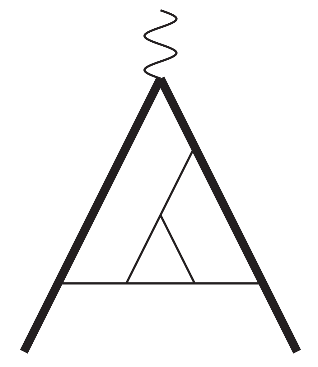
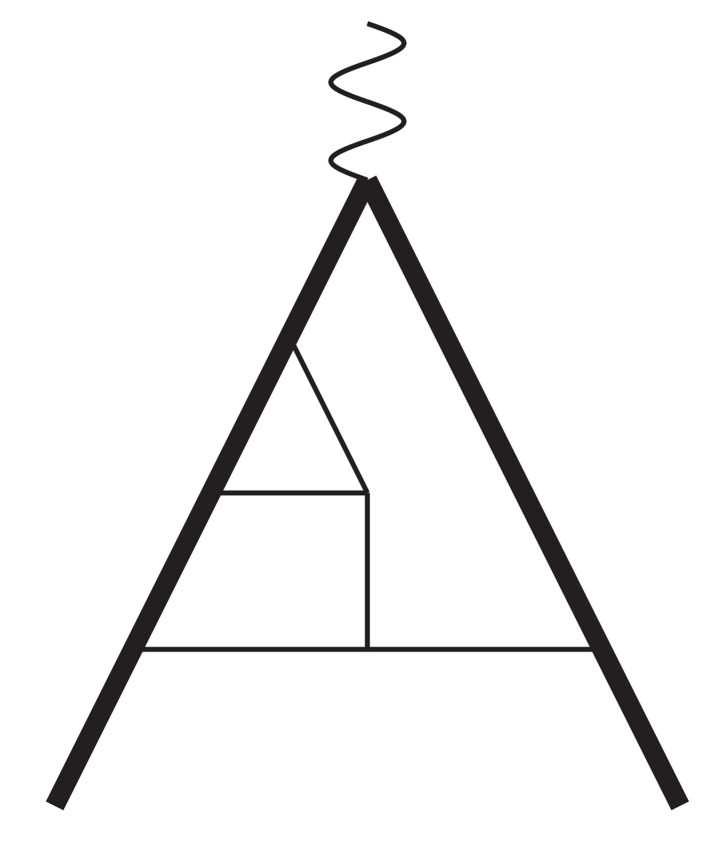
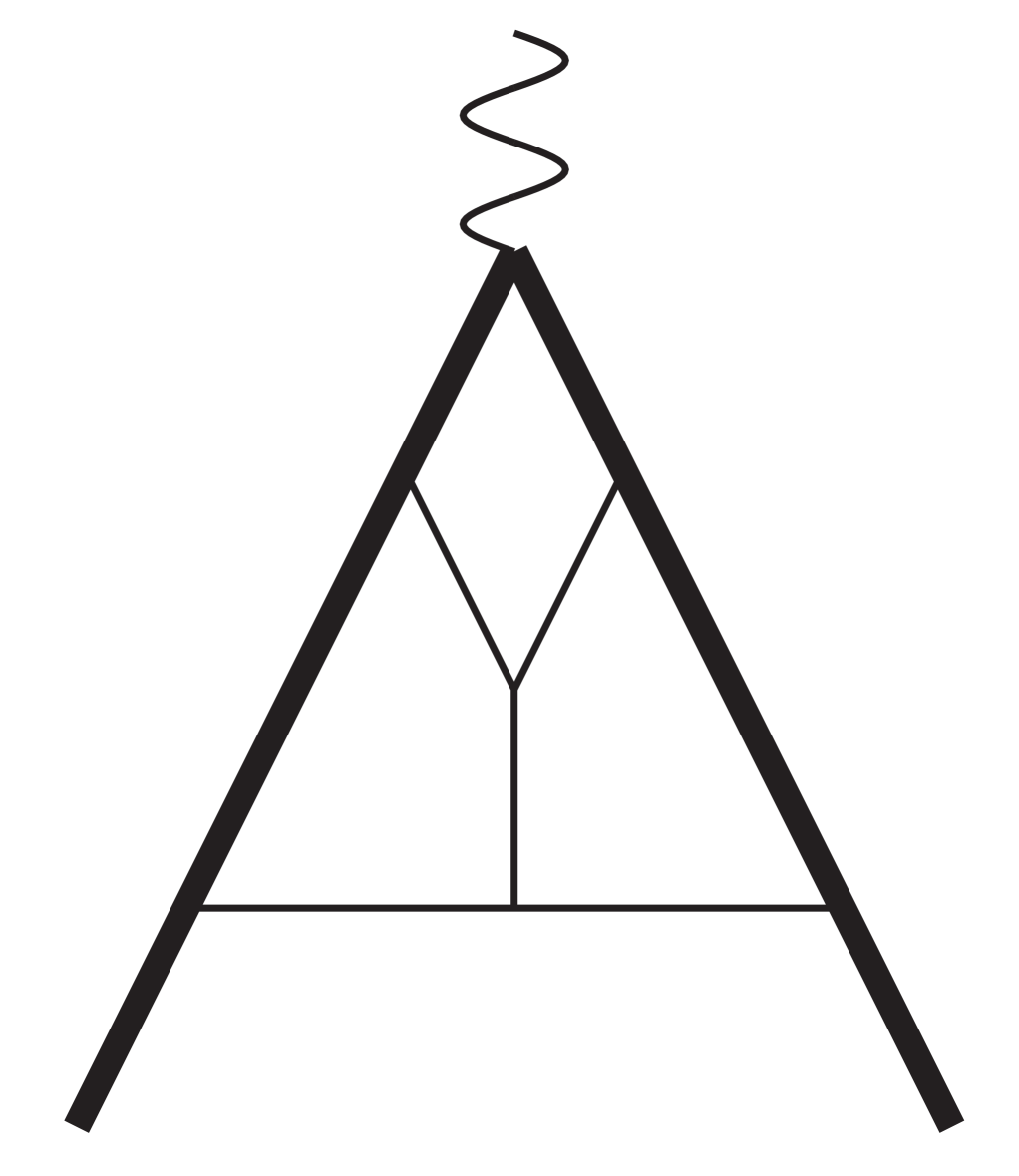
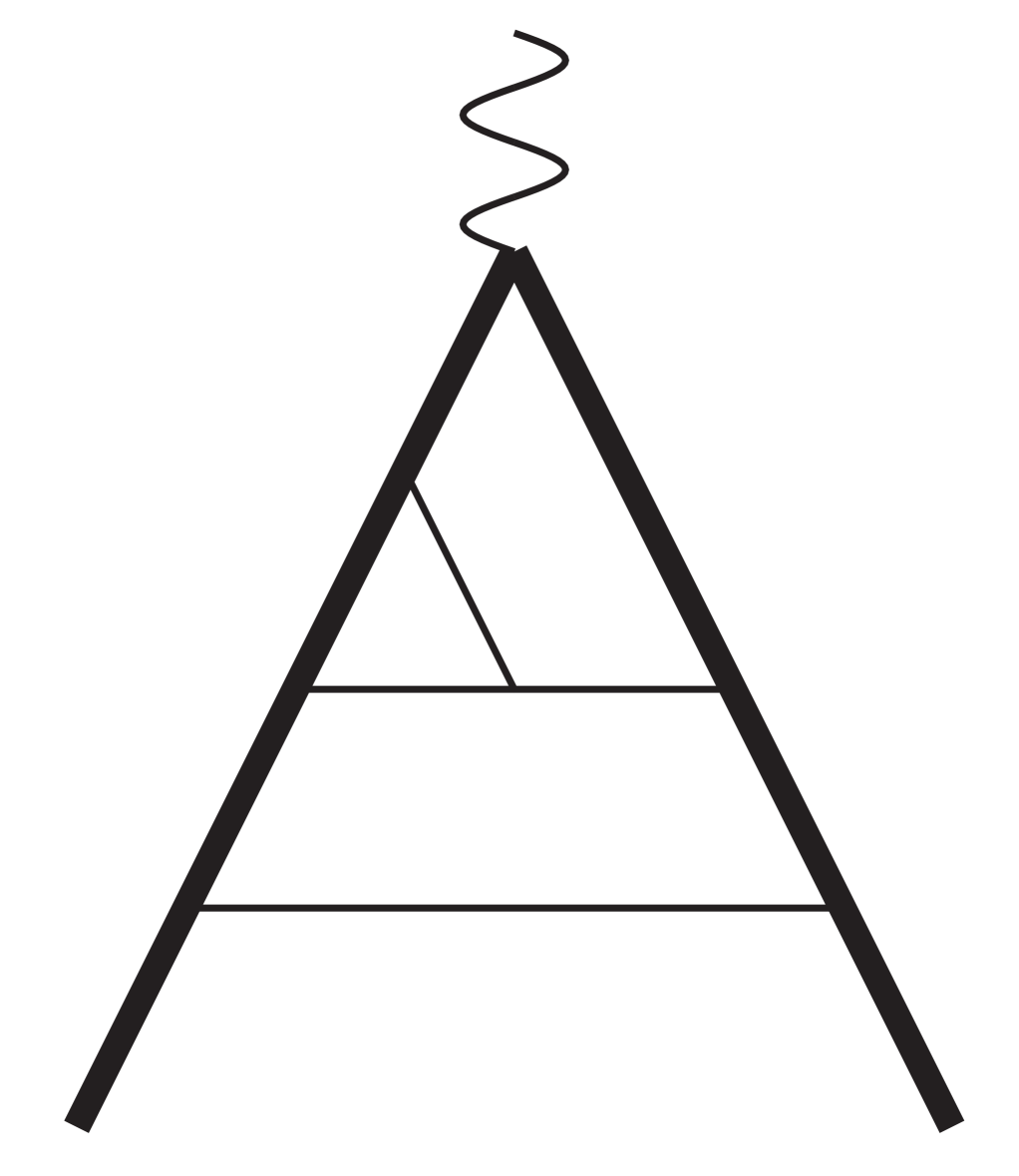
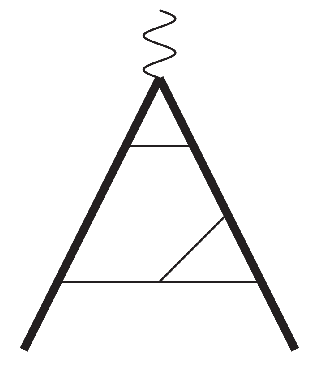
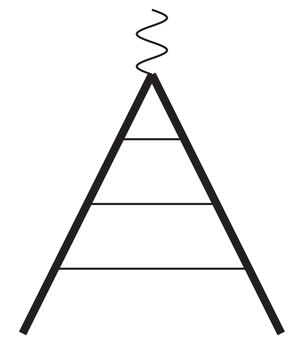
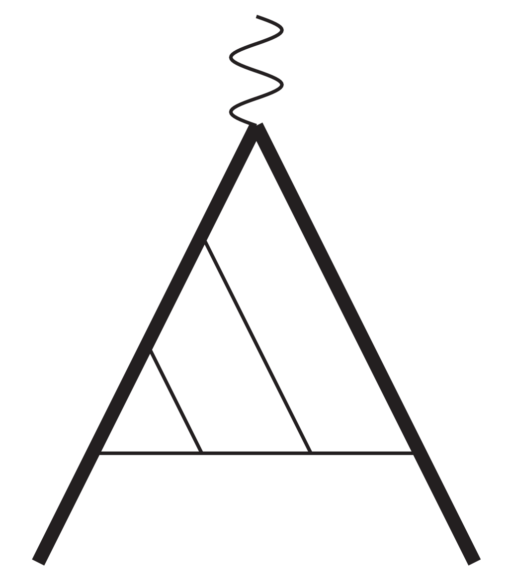
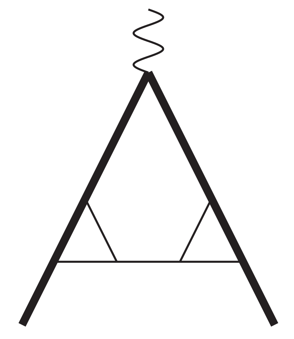
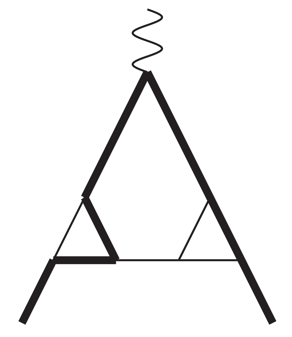
Figure 1: The color–planar topologies

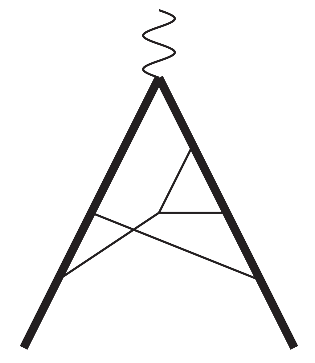
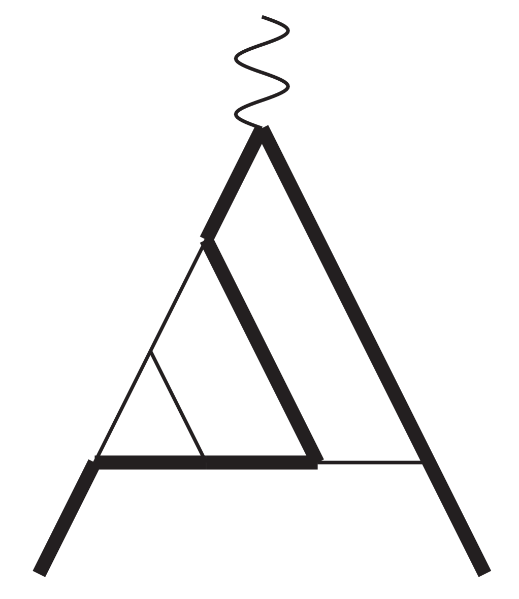
In the color–planar limit, the families of integrals can be represented by eight topologies, shown in Figure 1, whereas for the complete light quark contributions, three more topologies are required, cf. Figure 2. Note that, only sub-topologies with a maximum of eight propagators contribute in the latter scenario.
Refer to caption
Refer to caption
Refer to caption
Figure 2: The nlsubscript𝑛𝑙n_{l} topologies

Finally, to compute the master integrals, we implemented the algorithm described in the previous section, applying it to all occurring systems of differential equations. This calculation is performed by intense use of HarmonicSums [93, 95, 96, 77, 94, 97], which uses the package Sigma [27, 28]. Finally we have checked all MIs numerically using FIESTA [98, 99, 100].

3.2 Ultraviolet renormalization and infrared structure

The UV renormalization of the form factors has been performed in a mixed scheme. The heavy quark mass and wave function have been renormalized in the on-shell (OS) renormalization scheme, while the strong coupling constant is renormalized in the MS¯¯MS\overline{\rm MS} scheme, where we set the universal factor Sε=exp(ε(γEln(4π))S_{\varepsilon}=\exp(-\varepsilon(\gamma_{E}-\ln(4\pi)) for each loop order to one at the end of the calculation. The required renormalization constants are available and are denoted by Zm,OSsubscript𝑍𝑚OSZ_{m,{\rm OS}} [101, 102, 103, 104, 105], Z2,OSsubscript𝑍2OSZ_{2,{\rm OS}} [101, 102, 103, 106] and Zassubscript𝑍subscript𝑎𝑠Z_{a_{s}} [107, 108, 109, 110, 111, 112, 113] for the heavy quark mass, wave function and strong coupling constant, respectively. The renormalization of the heavy-quark wave function and the strong coupling constant are multiplicative, while the renormalization of massive fermion lines has been taken care of by properly considering the counter terms.

Considering the high energy limit, the universal behavior of infrared (IR) singularities of the massive form factors was first investigated in [114]. Later in [115], a general argument was provided to factorize the IR singularities as a multiplicative renormalization constant. Its structure is constrained by the renormalization group equation (RGE), as follows,

FI=Z(μ)FIfin(μ),subscript𝐹𝐼𝑍𝜇superscriptsubscript𝐹𝐼fin𝜇F_{I}=Z(\mu)F_{I}^{\mathrm{fin}}(\mu)\,, (70)

where FIfinsuperscriptsubscript𝐹𝐼finF_{I}^{\mathrm{fin}} is finite as ε0𝜀0\varepsilon\rightarrow 0. The RGE for Z(μ)𝑍𝜇Z(\mu) reads

ddlnμlnZ(ε,x,m,μ)=Γ(x,m,μ).𝑑𝑑𝜇𝑍𝜀𝑥𝑚𝜇Γ𝑥𝑚𝜇\frac{d}{d\ln\mu}\ln Z(\varepsilon,x,m,\mu)=-\Gamma(x,m,\mu). (71)

Here ΓΓ\Gamma is the corresponding cusp anomalous dimension, which is by now available up to three–loop order [116, 117]. Note that Z𝑍Z is independent of the current. Both Z𝑍Z and ΓΓ\Gamma can be expanded in a perturbative series in αssubscript𝛼𝑠\alpha_{s} as follows

Z=n=0(αs4π)nZ(n),Γ=n=0(αs4π)n+1Γn,formulae-sequence𝑍superscriptsubscript𝑛0superscriptsubscript𝛼𝑠4𝜋𝑛superscript𝑍𝑛Γsuperscriptsubscript𝑛0superscriptsubscript𝛼𝑠4𝜋𝑛1subscriptΓ𝑛Z=\sum_{n=0}^{\infty}\left(\frac{\alpha_{s}}{4\pi}\right)^{n}Z^{(n)}\,,\qquad\Gamma=\sum_{n=0}^{\infty}\left(\frac{\alpha_{s}}{4\pi}\right)^{n+1}\Gamma_{n}, (72)

and the solution for Eq. (71) up to 𝒪(αs3)𝒪superscriptsubscript𝛼𝑠3{\cal O}(\alpha_{s}^{3}) is

Z𝑍\displaystyle Z =1+(αs4π)[Γ02ε]+(αs4π)2[1ε2(Γ028β0Γ04)+Γ14ε]absent1subscript𝛼𝑠4𝜋delimited-[]subscriptΓ02𝜀superscriptsubscript𝛼𝑠4𝜋2delimited-[]1superscript𝜀2superscriptsubscriptΓ028subscript𝛽0subscriptΓ04subscriptΓ14𝜀\displaystyle=1+\left(\frac{\alpha_{s}}{4\pi}\right)\Bigg{[}\frac{\Gamma_{0}}{2\varepsilon}\Bigg{]}+\left(\frac{\alpha_{s}}{4\pi}\right)^{2}\Bigg{[}\frac{1}{\varepsilon^{2}}\Big{(}\frac{\Gamma_{0}^{2}}{8}-\frac{\beta_{0}\Gamma_{0}}{4}\Big{)}+\frac{\Gamma_{1}}{4\varepsilon}\Bigg{]}
+(αs4π)3[1ε3(Γ0348β0Γ028+β02Γ06)+1ε2(Γ0Γ18β1Γ06)+1ε(Γ26)]+𝒪(αs4).superscriptsubscript𝛼𝑠4𝜋3delimited-[]1superscript𝜀3superscriptsubscriptΓ0348subscript𝛽0superscriptsubscriptΓ028superscriptsubscript𝛽02subscriptΓ061superscript𝜀2subscriptΓ0subscriptΓ18subscript𝛽1subscriptΓ061𝜀subscriptΓ26𝒪superscriptsubscript𝛼𝑠4\displaystyle+\left(\frac{\alpha_{s}}{4\pi}\right)^{3}\bigg{[}\frac{1}{\varepsilon^{3}}\left(\frac{\Gamma_{0}^{3}}{48}-\frac{\beta_{0}\Gamma_{0}^{2}}{8}+\frac{\beta_{0}^{2}\Gamma_{0}}{6}\right)+\frac{1}{\varepsilon^{2}}\left(\frac{\Gamma_{0}\Gamma_{1}}{8}-\frac{\beta_{1}\Gamma_{0}}{6}\right)+\frac{1}{\varepsilon}\left(\frac{\Gamma_{2}}{6}\right)\bigg{]}+{\cal O}(\alpha_{s}^{4})\,. (73)

4 The Three-Loop Vector Form Factors

We apply our algorithm to the single scale and first order factorizable system of differential equations which are relevant for the color–planar and the complete light quark contributions to the heavy quark form factors. One obtains the solutions for all contributing integrals in Laurent series expansion up to the required order in ε𝜀\varepsilon .

Finally, using the results for the integrals, we obtain the color–planar and complete light quark (nlsubscript𝑛𝑙n_{l}) non–singlet contributions of the three-loop massive form factors for the vector current. Due to the substantial length of the expressions, we provide them as supplemental material along with this publication. In the following we only present expansions of the form factors in different kinematic limits and give numerical results for the whole kinematic region. Here the following abbreviation is used

c1=12ζ2ln2(2)+ln4(2)+24Li4(12),subscript𝑐112subscript𝜁2superscript22superscript4224Lsubscripti412c_{1}=12\zeta_{2}\ln^{2}(2)+\ln^{4}(2)+24{\rm Li}_{4}\left(\frac{1}{2}\right), (74)

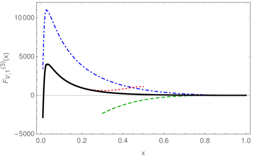
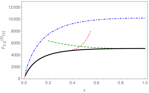
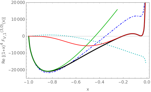
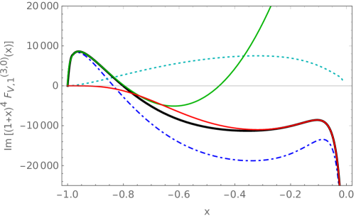
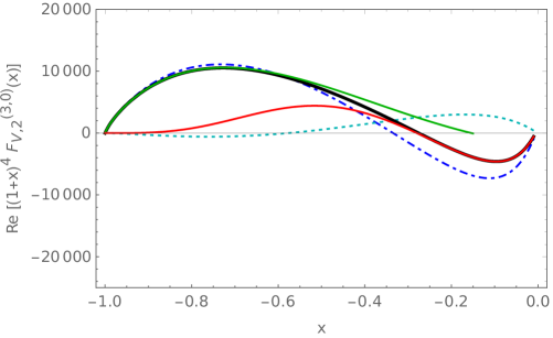
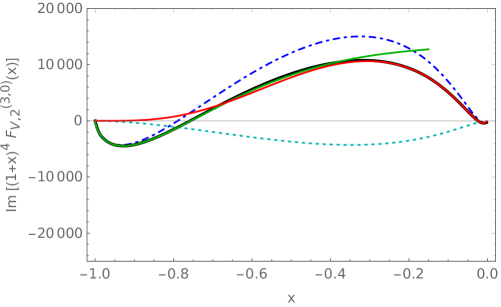
as mentioned in [48] and Lik(x)subscriptLi𝑘𝑥{\rm Li}_{k}(x) denotes the polylogarithm [119, 118]. In Figures 3 we illustrate the behavior of the O(ε0)𝑂superscript𝜀0O(\varepsilon^{0}) parts of the vector form factors as a function of x[0,1]𝑥01x\in[0,1]. We also show their small- and large-x𝑥x expansions. The latter representations are obtained using HarmonicSums. For the numerical evaluation of the HPLs and the cyclotomic HPLs we use the GiNaC package [120, 121] and the FORTRAN-codes HPOLY.f [84] and CPOLY.f.

We present now the expansion of the form factors in different kinematic regions.

4.1 The low energy region 𝒙𝟏bold-→𝒙1x\rightarrow 1

In the static limit, i.e. q20superscript𝑞20q^{2}\rightarrow 0, we define y=1x𝑦1𝑥y=1-x and expand the form factors around y=0𝑦0y=0. In this region, the electric component of the vector form factor vanishes. The 𝒪(y2)𝒪superscript𝑦2{\cal O}(y^{2}) contribution of the electric component of the three loop vector form factor (FV,1(3)superscriptsubscript𝐹𝑉13F_{V,1}^{(3)}) is given by

FV,1(3)y2similar-to-or-equalssuperscriptsubscript𝐹𝑉13superscript𝑦2\displaystyle{F}_{V,1}^{(3)}\simeq y^{2} [NC3{1ε312181+1ε2(1340243+4427ζ2)+1ε(4735468081ζ2+83ζ22+1027ζ3)\displaystyle\Bigg{[}N_{C}^{3}\bigg{\{}\frac{1}{\varepsilon^{3}}\frac{121}{81}+\frac{1}{\varepsilon^{2}}\bigg{(}-\frac{1340}{243}+\frac{44}{27}\zeta_{2}\bigg{)}+\frac{1}{\varepsilon}\bigg{(}\frac{473}{54}-\frac{680}{81}\zeta_{2}+\frac{8}{3}\zeta_{2}^{2}+\frac{10}{27}\zeta_{3}\bigg{)}
+(496156369984+8977486ζ22809ζ227127324ζ3+923ζ2ζ3+5ζ5)}+CF2nlTF{1ε289\displaystyle+\bigg{(}\frac{4961563}{69984}+\frac{8977}{486}\zeta_{2}-\frac{280}{9}\zeta_{2}^{2}-\frac{7127}{324}\zeta_{3}+\frac{92}{3}\zeta_{2}\zeta_{3}+5\zeta_{5}\bigg{)}\bigg{\}}+C_{F}^{2}n_{l}T_{F}\bigg{\{}\frac{1}{\varepsilon^{2}}\ \frac{8}{9}
1ε(11027329ζ3)+(310716264c191967681ζ2+35369ln(2)ζ2+179215ζ2211009ζ3)}\displaystyle-\frac{1}{\varepsilon}\bigg{(}\frac{110}{27}-\frac{32}{9}\zeta_{3}\bigg{)}+\bigg{(}\frac{3107}{162}-\frac{64c_{1}}{9}-\frac{19676}{81}\zeta_{2}+\frac{3536}{9}\ln(2)\zeta_{2}+\frac{1792}{15}\zeta_{2}^{2}-\frac{1100}{9}\zeta_{3}\bigg{)}\bigg{\}}
+CACFnlTF{1ε317681+1ε2(15522433227ζ2)+1ε(1556243+32081ζ211227ζ3)\displaystyle+C_{A}C_{F}n_{l}T_{F}\bigg{\{}-\frac{1}{\varepsilon^{3}}\frac{176}{81}+\frac{1}{\varepsilon^{2}}\bigg{(}\frac{1552}{243}-\frac{32}{27}\zeta_{2}\bigg{)}+\frac{1}{\varepsilon}\bigg{(}-\frac{1556}{243}+\frac{320}{81}\zeta_{2}-\frac{112}{27}\zeta_{3}\bigg{)}
+(2606442187+32c19+10474243ζ217689ln(2)ζ2140845ζ22+162227ζ3)}\displaystyle+\bigg{(}-\frac{260644}{2187}+\frac{32c_{1}}{9}+\frac{10474}{243}\zeta_{2}-\frac{1768}{9}\ln(2)\zeta_{2}-\frac{1408}{45}\zeta_{2}^{2}+\frac{1622}{27}\zeta_{3}\bigg{)}\bigg{\}}
+CFnl2TF2{1ε332811ε21602431ε32243+(295242187+92881ζ2+44881ζ3)}subscript𝐶𝐹superscriptsubscript𝑛𝑙2superscriptsubscript𝑇𝐹21superscript𝜀332811superscript𝜀21602431𝜀3224329524218792881subscript𝜁244881subscript𝜁3\displaystyle+C_{F}n_{l}^{2}T_{F}^{2}\bigg{\{}\frac{1}{\varepsilon^{3}}\frac{32}{81}-\frac{1}{\varepsilon^{2}}-\frac{160}{243}-\frac{1}{\varepsilon}-\frac{32}{243}+\bigg{(}\frac{29524}{2187}+\frac{928}{81}\zeta_{2}+\frac{448}{81}\zeta_{3}\bigg{)}\bigg{\}}
+CFnhnlTF2{1ε1627ζ2+(10088243+178481ζ2+16ln(2)ζ272481ζ3)}].\displaystyle+C_{F}n_{h}n_{l}T_{F}^{2}\bigg{\{}-\frac{1}{\varepsilon}\frac{16}{27}\zeta_{2}+\bigg{(}-\frac{10088}{243}+\frac{1784}{81}\zeta_{2}+16\ln(2)\zeta_{2}-\frac{724}{81}\zeta_{3}\bigg{)}\bigg{\}}\Bigg{]}\,. (75)

Here CA=NC,CF=(NC21)/(2NC),TF=1/2formulae-sequencesubscript𝐶𝐴subscript𝑁𝐶formulae-sequencesubscript𝐶𝐹superscriptsubscript𝑁𝐶212subscript𝑁𝐶subscript𝑇𝐹12C_{A}=N_{C},C_{F}=(N_{C}^{2}-1)/(2N_{C}),T_{F}=1/2 and NCsubscript𝑁𝐶N_{C} denotes the number of colors for SU(NC)𝑆𝑈subscript𝑁𝐶SU(N_{C}) with NC=3subscript𝑁𝐶3N_{C}=3 in case of QCD. The magnetic component of the vector form factor (FV,2)subscript𝐹𝑉2(F_{V,2}) is the anomalous magnetic moment of a heavy quark in this limit allowing for a cross-check of our computation with Ref. [122]. The form factor FV,2(3)superscriptsubscript𝐹𝑉23F_{V,2}^{(3)} up to order y2superscript𝑦2y^{2} reads

FV,2(3)similar-to-or-equalssuperscriptsubscript𝐹𝑉23absent\displaystyle{F}_{V,2}^{(3)}\simeq [NC3{104147648+9629ζ224ζ22+803ζ3+48ζ2ζ320ζ5}\displaystyle\Bigg{[}N_{C}^{3}\bigg{\{}\frac{104147}{648}+\frac{962}{9}\zeta_{2}-24\zeta_{2}^{2}+\frac{80}{3}\zeta_{3}+48\zeta_{2}\zeta_{3}-20\zeta_{5}\bigg{\}}
+CF2nlTF{25064c1950569ζ2+640ln(2)ζ2+3523ζ22192ζ3}superscriptsubscript𝐶𝐹2subscript𝑛𝑙subscript𝑇𝐹25064subscript𝑐1950569subscript𝜁26402subscript𝜁23523superscriptsubscript𝜁22192subscript𝜁3\displaystyle+C_{F}^{2}n_{l}T_{F}\bigg{\{}250-\frac{64c_{1}}{9}-\frac{5056}{9}\zeta_{2}+640\ln(2)\zeta_{2}+\frac{352}{3}\zeta_{2}^{2}-192\zeta_{3}\bigg{\}}
+CACFnlTF{3857681+32c19+12329ζ2320ln(2)ζ21763ζ22+3043ζ3}subscript𝐶𝐴subscript𝐶𝐹subscript𝑛𝑙subscript𝑇𝐹385768132subscript𝑐1912329subscript𝜁23202subscript𝜁21763superscriptsubscript𝜁223043subscript𝜁3\displaystyle+C_{A}C_{F}n_{l}T_{F}\bigg{\{}-\frac{38576}{81}+\frac{32c_{1}}{9}+\frac{1232}{9}\zeta_{2}-320\ln(2)\zeta_{2}-\frac{176}{3}\zeta_{2}^{2}+\frac{304}{3}\zeta_{3}\bigg{\}}
+CFnl2TF2{507281+1289ζ2}+CFnhnlTF2{195281+1289ζ2}]\displaystyle+C_{F}n_{l}^{2}T_{F}^{2}\bigg{\{}\frac{5072}{81}+\frac{128}{9}\zeta_{2}\bigg{\}}+C_{F}n_{h}n_{l}T_{F}^{2}\bigg{\{}-\frac{1952}{81}+\frac{128}{9}\zeta_{2}\bigg{\}}\Bigg{]}
+y2superscript𝑦2\displaystyle+y^{2} [1ε2(1118NC3+89CF2nlTF)+1ε(NC3{3112+23ζ2}163CF2nlTF)\displaystyle\Bigg{[}\frac{1}{\varepsilon^{2}}\Bigg{(}-\frac{11}{18}N_{C}^{3}+\frac{8}{9}C_{F}^{2}n_{l}T_{F}\Bigg{)}+\frac{1}{\varepsilon}\Bigg{(}N_{C}^{3}\bigg{\{}\frac{31}{12}+\frac{2}{3}\zeta_{2}\bigg{\}}-\frac{16}{3}C_{F}^{2}n_{l}T_{F}\Bigg{)}
+NC3{323646115552022849720ζ2+465ζ2240736ζ3725ζ2ζ3+6ζ5}superscriptsubscript𝑁𝐶3323646115552022849720subscript𝜁2465superscriptsubscript𝜁2240736subscript𝜁3725subscript𝜁2subscript𝜁36subscript𝜁5\displaystyle+N_{C}^{3}\bigg{\{}\frac{3236461}{155520}-\frac{22849}{720}\zeta_{2}+\frac{46}{5}\zeta_{2}^{2}-\frac{407}{36}\zeta_{3}-\frac{72}{5}\zeta_{2}\zeta_{3}+6\zeta_{5}\bigg{\}}
+CF2nlTF{1265390+736c1135+1218445ζ21609645ln(2)ζ2404845ζ22+6645ζ3}superscriptsubscript𝐶𝐹2subscript𝑛𝑙subscript𝑇𝐹1265390736subscript𝑐11351218445subscript𝜁216096452subscript𝜁2404845superscriptsubscript𝜁226645subscript𝜁3\displaystyle+C_{F}^{2}n_{l}T_{F}\bigg{\{}-\frac{12653}{90}+\frac{736c_{1}}{135}+\frac{12184}{45}\zeta_{2}-\frac{16096}{45}\ln(2)\zeta_{2}-\frac{4048}{45}\zeta_{2}^{2}+\frac{664}{5}\zeta_{3}\bigg{\}}
+CACFnlTF{26626243368c11359169ζ2+804845ln(2)ζ2+202445ζ223485ζ3}subscript𝐶𝐴subscript𝐶𝐹subscript𝑛𝑙subscript𝑇𝐹26626243368subscript𝑐11359169subscript𝜁28048452subscript𝜁2202445superscriptsubscript𝜁223485subscript𝜁3\displaystyle+C_{A}C_{F}n_{l}T_{F}\bigg{\{}\frac{26626}{243}-\frac{368c_{1}}{135}-\frac{916}{9}\zeta_{2}+\frac{8048}{45}\ln(2)\zeta_{2}+\frac{2024}{45}\zeta_{2}^{2}-\frac{348}{5}\zeta_{3}\bigg{\}}
CFnl2TF2{3736243+6427ζ2}+CFnhnlTF2{11824243803ζ2323ln(2)ζ2+569ζ3}].\displaystyle-C_{F}n_{l}^{2}T_{F}^{2}\bigg{\{}\frac{3736}{243}+\frac{64}{27}\zeta_{2}\bigg{\}}+C_{F}n_{h}n_{l}T_{F}^{2}\bigg{\{}\frac{11824}{243}-\frac{80}{3}\zeta_{2}-\frac{32}{3}\ln(2)\zeta_{2}+\frac{56}{9}\zeta_{3}\bigg{\}}\Bigg{]}\,. (76)

4.2 High energy region 𝒙𝟎bold-→𝒙0x\rightarrow 0

Here we present the expansion of the form factors FV,1(3)superscriptsubscript𝐹𝑉13F_{V,1}^{(3)} and FV,2(3)superscriptsubscript𝐹𝑉23F_{V,2}^{(3)} in the asymptotic limit i.e. for x0+𝑥superscript0x\rightarrow 0^{+} up to 𝒪(x2)𝒪superscript𝑥2{\cal O}(x^{2}). The abbreviation L𝐿L has been used to indicate ln(x)𝑥\ln(x).

FV,1(3)superscriptsubscript𝐹𝑉13\displaystyle{F}_{V,1}^{(3)} 1ε3[NC3{17527467L547L23L36}+CF2nlTF{83+16L3+8L23}\displaystyle\simeq\frac{1}{\varepsilon^{3}}\bigg{[}N_{C}^{3}\bigg{\{}-\frac{175}{27}-\frac{467L}{54}-\frac{7L^{2}}{3}-\frac{L^{3}}{6}\bigg{\}}+C_{F}^{2}n_{l}T_{F}\bigg{\{}\frac{8}{3}+\frac{16L}{3}+\frac{8L^{2}}{3}\bigg{\}}
+CACFnlTF{17627+176L27}+CFnl2TF2{322732L27}+x2(NC3{467L2728L23L3}\displaystyle+C_{A}C_{F}n_{l}T_{F}\bigg{\{}\frac{176}{27}+\frac{176L}{27}\bigg{\}}+C_{F}n_{l}^{2}T_{F}^{2}\bigg{\{}-\frac{32}{27}-\frac{32L}{27}\bigg{\}}+x^{2}\bigg{(}N_{C}^{3}\bigg{\{}-\frac{467L}{27}-\frac{28L^{2}}{3}-L^{3}\bigg{\}}
+CF2nlTF323L(1+L)+CACFnlTF352L27CFnl2TF264L27)]\displaystyle+C_{F}^{2}n_{l}T_{F}\frac{32}{3}L(1+L)+C_{A}C_{F}n_{l}T_{F}\frac{352L}{27}-C_{F}n_{l}^{2}T_{F}^{2}\frac{64L}{27}\bigg{)}\bigg{]}
+1ε2[NC3{1375162109ζ2+319ζ3+L(164516229ζ218+ζ3)+L2(9736ζ22)13L36L44}\displaystyle+\frac{1}{\varepsilon^{2}}\bigg{[}N_{C}^{3}\bigg{\{}\frac{1375}{162}-\frac{10}{9}\zeta_{2}+\frac{31}{9}\zeta_{3}+L\bigg{(}\frac{1645}{162}-\frac{29\zeta_{2}}{18}+\zeta_{3}\bigg{)}+L^{2}\bigg{(}-\frac{97}{36}-\frac{\zeta_{2}}{2}\bigg{)}-\frac{13L^{3}}{6}-\frac{L^{4}}{4}\bigg{\}}
+CF2nlTF{16983ζ2+L(2098ζ23)+8L29+4L33}+CACFnlTF{119281+169ζ2\displaystyle+C_{F}^{2}n_{l}T_{F}\bigg{\{}-\frac{16}{9}-\frac{8}{3}\zeta_{2}+L\bigg{(}-\frac{20}{9}-\frac{8\zeta_{2}}{3}\bigg{)}+\frac{8L^{2}}{9}+\frac{4L^{3}}{3}\bigg{\}}+C_{A}C_{F}n_{l}T_{F}\bigg{\{}-\frac{1192}{81}+\frac{16}{9}\zeta_{2}
169ζ3+L(133681+16ζ29)}+CFnl2TF2{16081+160L81}+x(NC3{14310L3+11L26\displaystyle-\frac{16}{9}\zeta_{3}+L\bigg{(}-\frac{1336}{81}+\frac{16\zeta_{2}}{9}\bigg{)}\bigg{\}}+C_{F}n_{l}^{2}T_{F}^{2}\bigg{\{}\frac{160}{81}+\frac{160L}{81}\bigg{\}}+x\bigg{(}N_{C}^{3}\bigg{\{}-\frac{14}{3}-\frac{10L}{3}+\frac{11L^{2}}{6}
+L32}+CF2nlTF{83(2+L)(1+L)})+x2(NC3{10318172L3275L46+L(8983324\displaystyle+\frac{L^{3}}{2}\bigg{\}}+C_{F}^{2}n_{l}T_{F}\bigg{\{}-\frac{8}{3}(-2+L)(1+L)\bigg{\}}\bigg{)}+x^{2}\bigg{(}N_{C}^{3}\bigg{\{}-\frac{103}{18}-\frac{172L^{3}}{27}-\frac{5L^{4}}{6}+L\bigg{(}\frac{8983}{324}
+34ζ23+6ζ3)+L2(4136+ζ2)+1049ζ2+1249ζ3}+CF2nlTF{43+32L29+16L33\displaystyle+\frac{34\zeta_{2}}{3}+6\zeta_{3}\bigg{)}+L^{2}\bigg{(}-\frac{41}{36}+\zeta_{2}\bigg{)}+\frac{104}{9}\zeta_{2}+\frac{124}{9}\zeta_{3}\bigg{\}}+C_{F}^{2}n_{l}T_{F}\bigg{\{}-\frac{4}{3}+\frac{32L^{2}}{9}+\frac{16L^{3}}{3}
+L(28932ζ23)163ζ2}+CACFnlTF{329329ζ2649ζ33104L8132L2932L327}\displaystyle+L\bigg{(}-\frac{28}{9}-\frac{32\zeta_{2}}{3}\bigg{)}-\frac{16}{3}\zeta_{2}\bigg{\}}+C_{A}C_{F}n_{l}T_{F}\bigg{\{}\frac{32}{9}-\frac{32}{9}\zeta_{2}-\frac{64}{9}\zeta_{3}-\frac{3104L}{81}-\frac{32L^{2}}{9}-\frac{32L^{3}}{27}\bigg{\}}
+CFnl2TF2{320L81})]+1ε[NC3{63754161108ζ2+6415ζ2255027ζ373ζ2ζ3+6ζ5+L(4369216\displaystyle+C_{F}n_{l}^{2}T_{F}^{2}\bigg{\{}\frac{320L}{81}\bigg{\}}\bigg{)}\bigg{]}+\frac{1}{\varepsilon}\bigg{[}N_{C}^{3}\bigg{\{}\frac{637}{54}-\frac{161}{108}\zeta_{2}+\frac{64}{15}\zeta_{2}^{2}-\frac{550}{27}\zeta_{3}-\frac{7}{3}\zeta_{2}\zeta_{3}+6\zeta_{5}+L\bigg{(}\frac{4369}{216}
161108ζ2+6415ζ2228118ζ3)+L2(46327+19ζ21211ζ32)+L3(1493ζ24)10L495L524}\displaystyle-\frac{161}{108}\zeta_{2}+\frac{64}{15}\zeta_{2}^{2}-\frac{281}{18}\zeta_{3}\bigg{)}+L^{2}\bigg{(}\frac{463}{27}+\frac{19\zeta_{2}}{12}-\frac{11\zeta_{3}}{2}\bigg{)}+L^{3}\bigg{(}\frac{14}{9}-\frac{3\zeta_{2}}{4}\bigg{)}-\frac{10L^{4}}{9}-\frac{5L^{5}}{24}\bigg{\}}
+CF2nlTF{47027+8ζ2163ζ3+L(119827+4ζ2316ζ33)+L2(9622720ζ23)\displaystyle+C_{F}^{2}n_{l}T_{F}\bigg{\{}-\frac{470}{27}+8\zeta_{2}-\frac{16}{3}\zeta_{3}+L\bigg{(}-\frac{1198}{27}+\frac{4\zeta_{2}}{3}-\frac{16\zeta_{3}}{3}\bigg{)}+L^{2}\bigg{(}-\frac{962}{27}-\frac{20\zeta_{2}}{3}\bigg{)}
82L394L49}+CACFnlTF{3568116027ζ2+49627ζ3+L(83681160ζ227+112ζ39)}\displaystyle-\frac{82L^{3}}{9}-\frac{4L^{4}}{9}\bigg{\}}+C_{A}C_{F}n_{l}T_{F}\bigg{\{}\frac{356}{81}-\frac{160}{27}\zeta_{2}+\frac{496}{27}\zeta_{3}+L\Bigl{(}\frac{836}{81}-\frac{160\zeta_{2}}{27}+\frac{112\zeta_{3}}{9}\Bigr{)}\bigg{\}}
+CFnl2TF2{3281+32L81}+CFnhnlTF2{169ζ2+169Lζ2}+x(NC3{10924696ζ21025ζ22\displaystyle+C_{F}n_{l}^{2}T_{F}^{2}\bigg{\{}\frac{32}{81}+\frac{32L}{81}\bigg{\}}+C_{F}n_{h}n_{l}T_{F}^{2}\bigg{\{}\frac{16}{9}\zeta_{2}+\frac{16}{9}L\zeta_{2}\bigg{\}}+x\bigg{(}N_{C}^{3}\bigg{\{}\frac{109}{2}-\frac{469}{6}\zeta_{2}-\frac{102}{5}\zeta_{2}^{2}
+124ζ3+L(457123233ζ21025ζ22+169ζ3)+L2(41671ζ22+48ζ3)+L3(4036ζ2)124subscript𝜁3𝐿457123233subscript𝜁21025superscriptsubscript𝜁22169subscript𝜁3superscript𝐿241671subscript𝜁2248subscript𝜁3superscript𝐿34036subscript𝜁2\displaystyle+124\zeta_{3}+L\bigg{(}\frac{457}{12}-\frac{323}{3}\zeta_{2}-\frac{102}{5}\zeta_{2}^{2}+169\zeta_{3}\bigg{)}+L^{2}\bigg{(}-\frac{41}{6}-\frac{71\zeta_{2}}{2}+48\zeta_{3}\bigg{)}+L^{3}\bigg{(}\frac{40}{3}-6\zeta_{2}\bigg{)}
+3L44}+CF2nlTF{4083ζ2+L(3238ζ23)+92L23+4L33})+x2(NC3{84209216\displaystyle+\frac{3L^{4}}{4}\bigg{\}}+C_{F}^{2}n_{l}T_{F}\bigg{\{}-40-\frac{8}{3}\zeta_{2}+L\bigg{(}-\frac{32}{3}-\frac{8\zeta_{2}}{3}\bigg{)}+\frac{92L^{2}}{3}+\frac{4L^{3}}{3}\bigg{\}}\bigg{)}+x^{2}\bigg{(}N_{C}^{3}\bigg{\{}-\frac{84209}{216}
+3297554ζ2+350915ζ225962754ζ314ζ2ζ3+20ζ5+L(33271216+25723ζ2+366115ζ22\displaystyle+\frac{32975}{54}\zeta_{2}+\frac{3509}{15}\zeta_{2}^{2}-\frac{59627}{54}\zeta_{3}-14\zeta_{2}\zeta_{3}+20\zeta_{5}+L\bigg{(}-\frac{33271}{216}+\frac{2572}{3}\zeta_{2}+\frac{3661}{15}\zeta_{2}^{2}
144509ζ3)+L2(19889108+988ζ231631ζ33)+L3(31061324+1001ζ218)17L46151L5180}\displaystyle-\frac{14450}{9}\zeta_{3}\bigg{)}+L^{2}\bigg{(}\frac{19889}{108}+\frac{988\zeta_{2}}{3}-\frac{1631\zeta_{3}}{3}\bigg{)}+L^{3}\bigg{(}-\frac{31061}{324}+\frac{1001\zeta_{2}}{18}\bigg{)}-\frac{17L^{4}}{6}-\frac{151L^{5}}{180}\bigg{\}}
+CF2nlTF{12+1123ζ2+323ζ3+L(254027+40ζ2)+L2(38842780ζ23)332L39\displaystyle+C_{F}^{2}n_{l}T_{F}\bigg{\{}12+\frac{112}{3}\zeta_{2}+\frac{32}{3}\zeta_{3}+L\bigg{(}-\frac{2540}{27}+40\zeta_{2}\bigg{)}+L^{2}\bigg{(}-\frac{3884}{27}-\frac{80\zeta_{2}}{3}\bigg{)}-\frac{332L^{3}}{9}
16L49}+CACFnlTF{32027+32027ζ2+64027ζ3+L(311281+224ζ39)+320L227+320L381}\displaystyle-\frac{16L^{4}}{9}\bigg{\}}+C_{A}C_{F}n_{l}T_{F}\bigg{\{}-\frac{320}{27}+\frac{320}{27}\zeta_{2}+\frac{640}{27}\zeta_{3}+L\bigg{(}\frac{3112}{81}+\frac{224\zeta_{3}}{9}\bigg{)}+\frac{320L^{2}}{27}+\frac{320L^{3}}{81}\bigg{\}}
+CFnl2TF2{64L81}+CFnhnlTF2{329Lζ2})]+[NC3{5542672916+23773216ζ2172730ζ22\displaystyle+C_{F}n_{l}^{2}T_{F}^{2}\bigg{\{}\frac{64L}{81}\bigg{\}}+C_{F}n_{h}n_{l}T_{F}^{2}\bigg{\{}\frac{32}{9}L\zeta_{2}\bigg{\}}\bigg{)}\bigg{]}+\bigg{[}N_{C}^{3}\bigg{\{}-\frac{554267}{2916}+\frac{23773}{216}\zeta_{2}-\frac{1727}{30}\zeta_{2}^{2}
+8156315ζ23+33197162ζ3+1133ζ2ζ3163ζ328753ζ5+L(669127583231609324ζ27110ζ22\displaystyle+\frac{8156}{315}\zeta_{2}^{3}+\frac{33197}{162}\zeta_{3}+\frac{113}{3}\zeta_{2}\zeta_{3}-\frac{16}{3}\zeta_{3}^{2}-\frac{875}{3}\zeta_{5}+L\bigg{(}-\frac{669127}{5832}-\frac{31609}{324}\zeta_{2}-\frac{71}{10}\zeta_{2}^{2}
+429754ζ3136ζ2ζ3+15ζ5)+L2(153536+59372ζ24ζ2262936ζ3)+L3(6373324+37ζ212\displaystyle+\frac{4297}{54}\zeta_{3}-\frac{13}{6}\zeta_{2}\zeta_{3}+15\zeta_{5}\bigg{)}+L^{2}\bigg{(}\frac{1535}{36}+\frac{593}{72}\zeta_{2}-4\zeta_{2}^{2}-\frac{629}{36}\zeta_{3}\bigg{)}+L^{3}\bigg{(}\frac{6373}{324}+\frac{37\zeta_{2}}{12}
49ζ36)+L4(11414322ζ23)3L58L68}+CF2nlTF{20118164c199623ζ2\displaystyle-\frac{49\zeta_{3}}{6}\bigg{)}+L^{4}\bigg{(}\frac{1141}{432}-\frac{2\zeta_{2}}{3}\bigg{)}-\frac{3L^{5}}{8}-\frac{L^{6}}{8}\bigg{\}}+C_{F}^{2}n_{l}T_{F}\bigg{\{}-\frac{2011}{81}-\frac{64c_{1}}{9}-\frac{962}{3}\zeta_{2}
+4483ln(2)ζ2+1223245ζ22+27529ζ348ζ2ζ3+40ζ5+L(18812816829ζ2+39215ζ22\displaystyle+\frac{448}{3}\ln(2)\zeta_{2}+\frac{12232}{45}\zeta_{2}^{2}+\frac{2752}{9}\zeta_{3}-48\zeta_{2}\zeta_{3}+40\zeta_{5}+L\bigg{(}-\frac{18812}{81}-\frac{682}{9}\zeta_{2}+\frac{392}{15}\zeta_{2}^{2}
+19769ζ3)+L2(1881781100ζ23+232ζ39)+L3(20322758ζ29)355L427L5}\displaystyle+\frac{1976}{9}\zeta_{3}\bigg{)}+L^{2}\bigg{(}-\frac{18817}{81}-\frac{100\zeta_{2}}{3}+\frac{232\zeta_{3}}{9}\bigg{)}+L^{3}\bigg{(}-\frac{2032}{27}-\frac{58\zeta_{2}}{9}\bigg{)}-\frac{355L^{4}}{27}-L^{5}\bigg{\}}
+CACFnlTF{259150729+32c19+300881ζ22243ln(2)ζ2728845ζ223112081ζ3+83ζ2ζ3\displaystyle+C_{A}C_{F}n_{l}T_{F}\bigg{\{}\frac{259150}{729}+\frac{32c_{1}}{9}+\frac{3008}{81}\zeta_{2}-\frac{224}{3}\ln(2)\zeta_{2}-\frac{7288}{45}\zeta_{2}^{2}-\frac{31120}{81}\zeta_{3}+\frac{8}{3}\zeta_{2}\zeta_{3}
+5963ζ5+L(309838729+1172881ζ28815ζ2214489ζ3)+L2(1175281+32ζ2316ζ3)5963subscript𝜁5𝐿3098387291172881subscript𝜁28815superscriptsubscript𝜁2214489subscript𝜁3superscript𝐿2117528132subscript𝜁2316subscript𝜁3\displaystyle+\frac{596}{3}\zeta_{5}+L\bigg{(}\frac{309838}{729}+\frac{11728}{81}\zeta_{2}-\frac{88}{15}\zeta_{2}^{2}-\frac{1448}{9}\zeta_{3}\bigg{)}+L^{2}\bigg{(}\frac{11752}{81}+\frac{32\zeta_{2}}{3}-16\zeta_{3}\bigg{)}
+L3(19488116ζ29)+44L427}+CFnl2TF2{2934472997681ζ2+92845ζ22+2569ζ3\displaystyle+L^{3}\bigg{(}\frac{1948}{81}-\frac{16\zeta_{2}}{9}\bigg{)}+\frac{44L^{4}}{27}\bigg{\}}+C_{F}n_{l}^{2}T_{F}^{2}\bigg{\{}-\frac{29344}{729}-\frac{976}{81}\zeta_{2}+\frac{928}{45}\zeta_{2}^{2}+\frac{256}{9}\zeta_{3}
+L(39352729608ζ22764ζ327)+L2(16248132ζ29)304L3818L427}\displaystyle+L\bigg{(}-\frac{39352}{729}-\frac{608\zeta_{2}}{27}-\frac{64\zeta_{3}}{27}\bigg{)}+L^{2}\bigg{(}-\frac{1624}{81}-\frac{32\zeta_{2}}{9}\bigg{)}-\frac{304L^{3}}{81}-\frac{8L^{4}}{27}\bigg{\}}
+CFnhnlTF2{507227+155281ζ2643ζ224169ζ3+L(74088148ζ2416ζ327)\displaystyle+C_{F}n_{h}n_{l}T_{F}^{2}\bigg{\{}-\frac{5072}{27}+\frac{1552}{81}\zeta_{2}-\frac{64}{3}\zeta_{2}^{2}-\frac{416}{9}\zeta_{3}+L\bigg{(}-\frac{7408}{81}-48\zeta_{2}-\frac{416\zeta_{3}}{27}\bigg{)}
+L2(32488164ζ29)608L38116L427}+x(NC3{149093324+122195108ζ2+529160ζ22\displaystyle+L^{2}\bigg{(}-\frac{3248}{81}-\frac{64\zeta_{2}}{9}\bigg{)}-\frac{608L^{3}}{81}-\frac{16L^{4}}{27}\bigg{\}}+x\bigg{(}N_{C}^{3}\bigg{\{}-\frac{149093}{324}+\frac{122195}{108}\zeta_{2}+\frac{5291}{60}\zeta_{2}^{2}
479435ζ23246479ζ3278ζ2ζ3+18ζ32+2154ζ5+L(145181+822112ζ2+4012ζ2233913ζ3\displaystyle-\frac{4794}{35}\zeta_{2}^{3}-\frac{24647}{9}\zeta_{3}-278\zeta_{2}\zeta_{3}+18\zeta_{3}^{2}+2154\zeta_{5}+L\bigg{(}-\frac{1451}{81}+\frac{8221}{12}\zeta_{2}+\frac{401}{2}\zeta_{2}^{2}-\frac{3391}{3}\zeta_{3}
+12ζ2ζ3+96ζ5)+L2(13525108+223ζ2+3065ζ22130ζ3)+L3(3095108197ζ212+40ζ3)\displaystyle+12\zeta_{2}\zeta_{3}+96\zeta_{5}\bigg{)}+L^{2}\bigg{(}-\frac{13525}{108}+\frac{22}{3}\zeta_{2}+\frac{306}{5}\zeta_{2}^{2}-130\zeta_{3}\bigg{)}+L^{3}\bigg{(}-\frac{3095}{108}-\frac{197\zeta_{2}}{12}+40\zeta_{3}\bigg{)}
+L4(1319729ζ2)+5L58}+CF2nlTF{16769+128c13+68009ζ23328ln(2)ζ2209645ζ22\displaystyle+L^{4}\bigg{(}\frac{1319}{72}-9\zeta_{2}\bigg{)}+\frac{5L^{5}}{8}\bigg{\}}+C_{F}^{2}n_{l}T_{F}\bigg{\{}-\frac{1676}{9}+\frac{128c_{1}}{3}+\frac{6800}{9}\zeta_{2}-3328\ln(2)\zeta_{2}-\frac{2096}{45}\zeta_{2}^{2}
+45289ζ3+128ζ2ζ313123ζ5+L(790958369ζ2+137615ζ22+2243ζ3)+L2(34169356ζ29\displaystyle+\frac{4528}{9}\zeta_{3}+128\zeta_{2}\zeta_{3}-\frac{1312}{3}\zeta_{5}+L\bigg{(}\frac{790}{9}-\frac{5836}{9}\zeta_{2}+\frac{1376}{15}\zeta_{2}^{2}+\frac{224}{3}\zeta_{3}\bigg{)}+L^{2}\bigg{(}\frac{3416}{9}-\frac{356\zeta_{2}}{9}
+16ζ33)+L3(34362716ζ2)+352L427+4L59}+CACFnlTF{973848164c133397627ζ2\displaystyle+\frac{16\zeta_{3}}{3}\bigg{)}+L^{3}\bigg{(}\frac{3436}{27}-16\zeta_{2}\bigg{)}+\frac{352L^{4}}{27}+\frac{4L^{5}}{9}\bigg{\}}+C_{A}C_{F}n_{l}T_{F}\bigg{\{}\frac{97384}{81}-\frac{64c_{1}}{3}-\frac{33976}{27}\zeta_{2}
+1664ln(2)ζ2+347245ζ22+144409ζ364ζ2ζ318403ζ5+L(346648115763ζ2+94415ζ22\displaystyle+1664\ln(2)\zeta_{2}+\frac{3472}{45}\zeta_{2}^{2}+\frac{14440}{9}\zeta_{3}-64\zeta_{2}\zeta_{3}-\frac{1840}{3}\zeta_{5}+L\bigg{(}-\frac{34664}{81}-\frac{1576}{3}\zeta_{2}+\frac{944}{15}\zeta_{2}^{2}
+560ζ3)+L2(104271040ζ29+232ζ33)+L3(160278ζ2)116L4272L59}\displaystyle+560\zeta_{3}\bigg{)}+L^{2}\bigg{(}\frac{104}{27}-\frac{1040\zeta_{2}}{9}+\frac{232\zeta_{3}}{3}\bigg{)}+L^{3}\bigg{(}-\frac{160}{27}-8\zeta_{2}\bigg{)}-\frac{116L^{4}}{27}-\frac{2L^{5}}{9}\bigg{\}}
+CFnl2TF2{1129681195227ζ21289ζ3+L(872081+64ζ29)+592L227+32L327}subscript𝐶𝐹superscriptsubscript𝑛𝑙2superscriptsubscript𝑇𝐹21129681195227subscript𝜁21289subscript𝜁3𝐿87208164subscript𝜁29592superscript𝐿22732superscript𝐿327\displaystyle+C_{F}n_{l}^{2}T_{F}^{2}\bigg{\{}-\frac{11296}{81}-\frac{1952}{27}\zeta_{2}-\frac{128}{9}\zeta_{3}+L\bigg{(}\frac{8720}{81}+\frac{64\zeta_{2}}{9}\bigg{)}+\frac{592L^{2}}{27}+\frac{32L^{3}}{27}\bigg{\}}
+CFnhnlTF2{540881+1139227ζ2+16649ζ3+L(1513681+896ζ29)+3104L227+448L327})\displaystyle+C_{F}n_{h}n_{l}T_{F}^{2}\bigg{\{}-\frac{5408}{81}+\frac{11392}{27}\zeta_{2}+\frac{1664}{9}\zeta_{3}+L\bigg{(}\frac{15136}{81}+\frac{896\zeta_{2}}{9}\bigg{)}+\frac{3104L^{2}}{27}+\frac{448L^{3}}{27}\bigg{\}}\bigg{)}
+x2(NC3{5219472166272521648ζ212090790ζ22+516347315ζ23+165509281ζ3+245029ζ2ζ3\displaystyle+x^{2}\bigg{(}N_{C}^{3}\bigg{\{}\frac{521947}{216}-\frac{6272521}{648}\zeta_{2}-\frac{120907}{90}\zeta_{2}^{2}+\frac{516347}{315}\zeta_{2}^{3}+\frac{1655092}{81}\zeta_{3}+\frac{24502}{9}\zeta_{2}\zeta_{3}
+93ζ3218684ζ5+L(72409129161172257216ζ2123765ζ22+35265427ζ3+2233ζ2ζ359983ζ5)93superscriptsubscript𝜁3218684subscript𝜁5𝐿72409129161172257216subscript𝜁2123765superscriptsubscript𝜁2235265427subscript𝜁32233subscript𝜁2subscript𝜁359983subscript𝜁5\displaystyle+93\zeta_{3}^{2}-18684\zeta_{5}+L\Bigl{(}\frac{724091}{2916}-\frac{1172257}{216}\zeta_{2}-\frac{12376}{5}\zeta_{2}^{2}+\frac{352654}{27}\zeta_{3}+\frac{223}{3}\zeta_{2}\zeta_{3}-\frac{5998}{3}\zeta_{5}\bigg{)}
+L2(24851723531172ζ2857915ζ22+3835318ζ3)+L3(1165405194443ζ2544373ζ39)superscript𝐿224851723531172subscript𝜁2857915superscriptsubscript𝜁223835318subscript𝜁3superscript𝐿31165405194443subscript𝜁2544373subscript𝜁39\displaystyle+L^{2}\bigg{(}\frac{24851}{72}-\frac{35311}{72}\zeta_{2}-\frac{8579}{15}\zeta_{2}^{2}+\frac{38353}{18}\zeta_{3}\bigg{)}+L^{3}\bigg{(}\frac{1165405}{1944}-\frac{43\zeta_{2}}{54}-\frac{4373\zeta_{3}}{9}\bigg{)}
+L4(61187432+1711ζ218)541L554071L6180}+CF2nlTF{259519256c13+527149ζ2\displaystyle+L^{4}\bigg{(}-\frac{61187}{432}+\frac{1711\zeta_{2}}{18}\bigg{)}-\frac{541L^{5}}{540}-\frac{71L^{6}}{180}\bigg{\}}+C_{F}^{2}n_{l}T_{F}\bigg{\{}-\frac{25951}{9}-\frac{256c_{1}}{3}+\frac{52714}{9}\zeta_{2}
+7680ln(2)ζ2382445ζ22171523ζ330083ζ2ζ3+169283ζ5+L(11642081+432349ζ2\displaystyle+7680\ln(2)\zeta_{2}-\frac{3824}{45}\zeta_{2}^{2}-\frac{17152}{3}\zeta_{3}-\frac{3008}{3}\zeta_{2}\zeta_{3}+\frac{16928}{3}\zeta_{5}+L\bigg{(}\frac{116420}{81}+\frac{43234}{9}\zeta_{2}
1020815ζ221520ζ3)+L2(12741481+4160ζ29848ζ39)+L3(1378627+440ζ23)\displaystyle-\frac{10208}{15}\zeta_{2}^{2}-1520\zeta_{3}\bigg{)}+L^{2}\bigg{(}-\frac{127414}{81}+\frac{4160\zeta_{2}}{9}-\frac{848\zeta_{3}}{9}\bigg{)}+L^{3}\bigg{(}-\frac{13786}{27}+\frac{440\zeta_{2}}{3}\bigg{)}
2398L427124L515}+CACFnlTF{29957681+128c13+16361227ζ23840ln(2)ζ2\displaystyle-\frac{2398L^{4}}{27}-\frac{124L^{5}}{15}\bigg{\}}+C_{A}C_{F}n_{l}T_{F}\bigg{\{}-\frac{299576}{81}+\frac{128c_{1}}{3}+\frac{163612}{27}\zeta_{2}-3840\ln(2)\zeta_{2}
2058445ζ22114836881ζ3+45449ζ2ζ3+202243ζ5+L(1311029729+10980427ζ2552ζ22\displaystyle-\frac{20584}{45}\zeta_{2}^{2}-\frac{1148368}{81}\zeta_{3}+\frac{4544}{9}\zeta_{2}\zeta_{3}+\frac{20224}{3}\zeta_{5}+L\bigg{(}\frac{1311029}{729}+\frac{109804}{27}\zeta_{2}-552\zeta_{2}^{2}
187043ζ3)+L2(51829+1080ζ27792ζ39)+L3(22322243+2456ζ227)+232L49\displaystyle-\frac{18704}{3}\zeta_{3}\bigg{)}+L^{2}\bigg{(}-\frac{5182}{9}+1080\zeta_{2}-\frac{7792\zeta_{3}}{9}\bigg{)}+L^{3}\bigg{(}-\frac{22322}{243}+\frac{2456\zeta_{2}}{27}\bigg{)}+\frac{232L^{4}}{9}
+364L5135}+CFnl2TF2{829681+889681ζ2+185645ζ22+281627ζ3+L(1390407291408ζ227\displaystyle+\frac{364L^{5}}{135}\bigg{\}}+C_{F}n_{l}^{2}T_{F}^{2}\bigg{\{}\frac{8296}{81}+\frac{8896}{81}\zeta_{2}+\frac{1856}{45}\zeta_{2}^{2}+\frac{2816}{27}\zeta_{3}+L\bigg{(}-\frac{139040}{729}-\frac{1408\zeta_{2}}{27}
128ζ327)+L2(41608164ζ29)704L38116L427}+CFnhnlTF2{250408114665681ζ2\displaystyle-\frac{128\zeta_{3}}{27}\bigg{)}+L^{2}\bigg{(}-\frac{4160}{81}-\frac{64\zeta_{2}}{9}\bigg{)}-\frac{704L^{3}}{81}-\frac{16L^{4}}{27}\bigg{\}}+C_{F}n_{h}n_{l}T_{F}^{2}\bigg{\{}\frac{25040}{81}-\frac{146656}{81}\zeta_{2}
+2563ζ222585627ζ3+L(444834768ζ29+1472ζ327)+L2(5396881+256ζ29)2563superscriptsubscript𝜁222585627subscript𝜁3𝐿444834768subscript𝜁291472subscript𝜁327superscript𝐿25396881256subscript𝜁29\displaystyle+\frac{256}{3}\zeta_{2}^{2}-\frac{25856}{27}\zeta_{3}+L\bigg{(}-\frac{4448}{3}-\frac{4768\zeta_{2}}{9}+\frac{1472\zeta_{3}}{27}\bigg{)}+L^{2}\bigg{(}-\frac{53968}{81}+\frac{256\zeta_{2}}{9}\bigg{)}
7072L381+64L427})].\displaystyle-\frac{7072L^{3}}{81}+\frac{64L^{4}}{27}\bigg{\}}\bigg{)}\bigg{]}\,. (77)

In this limit, the electric component of the vector form factor i.e. FV,1subscript𝐹𝑉1F_{V,1} satisfies the Sudakov evolution equation. This behavior has been studied in detail in [54, 114, 55] accounting for the components known. The complete three-loop result has been given in [54] and partial four–loop results in [54, 55].

FV,2(3)superscriptsubscript𝐹𝑉23\displaystyle{F}_{V,2}^{(3)} 1ε2[x(NC3{14L317L23L3}+CF2nlTF163L(1+L))]+1ε[x(NC3{6+853ζ2\displaystyle\simeq\frac{1}{\varepsilon^{2}}\bigg{[}x\bigg{(}N_{C}^{3}\bigg{\{}-\frac{14L}{3}-\frac{17L^{2}}{3}-L^{3}\bigg{\}}+C_{F}^{2}n_{l}T_{F}\frac{16}{3}L(1+L)\bigg{)}\bigg{]}+\frac{1}{\varepsilon}\bigg{[}x\bigg{(}N_{C}^{3}\bigg{\{}-6+\frac{85}{3}\zeta_{2}
44ζ3+L(152+112ζ2342ζ3)+L2(173+9ζ2)23L333L42}+CF2nlTF{163ζ2\displaystyle-44\zeta_{3}+L\bigg{(}-\frac{15}{2}+\frac{112\zeta_{2}}{3}-42\zeta_{3}\bigg{)}+L^{2}\bigg{(}-\frac{17}{3}+9\zeta_{2}\bigg{)}-\frac{23L^{3}}{3}-\frac{3L^{4}}{2}\bigg{\}}+C_{F}^{2}n_{l}T_{F}\bigg{\{}\frac{16}{3}\zeta_{2}
+L(32+16ζ23)104L238L33})+x2(NC3{4663516ζ28165ζ22+944ζ3\displaystyle+L\bigg{(}-32+\frac{16\zeta_{2}}{3}\bigg{)}-\frac{104L^{2}}{3}-\frac{8L^{3}}{3}\bigg{\}}\bigg{)}+x^{2}\bigg{(}N_{C}^{3}\bigg{\{}\frac{466}{3}-516\zeta_{2}-\frac{816}{5}\zeta_{2}^{2}+944\zeta_{3}
+L(66752ζ28165ζ22+1328ζ3)+L2(163284ζ2+384ζ3)+L3(8448ζ2)}\displaystyle+L\bigg{(}66-752\zeta_{2}-\frac{816}{5}\zeta_{2}^{2}+1328\zeta_{3}\bigg{)}+L^{2}\bigg{(}-\frac{16}{3}-284\zeta_{2}+384\zeta_{3}\bigg{)}+L^{3}\bigg{(}84-48\zeta_{2}\bigg{)}\bigg{\}}
+CF2nlTF{323(1+L)(1+L)})]+[x(NC3{54833900554ζ2+32915ζ22+46973ζ3+154ζ2ζ3\displaystyle+C_{F}^{2}n_{l}T_{F}\bigg{\{}\frac{32}{3}(-1+L)(1+L)\bigg{\}}\bigg{)}\bigg{]}+\bigg{[}x\bigg{(}N_{C}^{3}\bigg{\{}\frac{548}{3}-\frac{39005}{54}\zeta_{2}+\frac{329}{15}\zeta_{2}^{2}+\frac{4697}{3}\zeta_{3}+154\zeta_{2}\zeta_{3}
732ζ5+L(225516241009ζ22465ζ22+7543ζ3)+L2(720154+133ζ2613ζ3)732subscript𝜁5𝐿225516241009subscript𝜁22465superscriptsubscript𝜁227543subscript𝜁3superscript𝐿2720154133subscript𝜁2613subscript𝜁3\displaystyle-732\zeta_{5}+L\bigg{(}\frac{2255}{162}-\frac{4100}{9}\zeta_{2}-\frac{246}{5}\zeta_{2}^{2}+\frac{754}{3}\zeta_{3}\bigg{)}+L^{2}\bigg{(}\frac{7201}{54}+\frac{133\zeta_{2}}{6}-13\zeta_{3}\bigg{)}
+L3(27727+19ζ22)227L4365L54}+CF2nlTF{163256c1954409ζ2+56323ln(2)ζ2\displaystyle+L^{3}\bigg{(}\frac{277}{27}+\frac{19\zeta_{2}}{2}\bigg{)}-\frac{227L^{4}}{36}-\frac{5L^{5}}{4}\bigg{\}}+C_{F}^{2}n_{l}T_{F}\bigg{\{}\frac{16}{3}-\frac{256c_{1}}{9}-\frac{5440}{9}\zeta_{2}+\frac{5632}{3}\ln(2)\zeta_{2}
+262415ζ2233289ζ3+L(41729+3176ζ29+416ζ33)+L2(2936956ζ23)832L39262415superscriptsubscript𝜁2233289subscript𝜁3𝐿417293176subscript𝜁29416subscript𝜁33superscript𝐿22936956subscript𝜁23832superscript𝐿39\displaystyle+\frac{2624}{15}\zeta_{2}^{2}-\frac{3328}{9}\zeta_{3}+L\Bigl{(}-\frac{4172}{9}+\frac{3176\zeta_{2}}{9}+\frac{416\zeta_{3}}{3}\Bigr{)}+L^{2}\Bigl{(}-\frac{2936}{9}-\frac{56\zeta_{2}}{3}\Bigr{)}-\frac{832L^{3}}{9}
80L49}+CACFnlTF{4963+128c19+1616027ζ228163ln(2)ζ296ζ2221923ζ3\displaystyle-\frac{80L^{4}}{9}\bigg{\}}+C_{A}C_{F}n_{l}T_{F}\bigg{\{}-\frac{496}{3}+\frac{128c_{1}}{9}+\frac{16160}{27}\zeta_{2}-\frac{2816}{3}\ln(2)\zeta_{2}-96\zeta_{2}^{2}-\frac{2192}{3}\zeta_{3}
+L(4432081+2336ζ29512ζ33)+L2(125627+80ζ23)+64L327}+CFnl2TF2{160027ζ2+2569ζ3\displaystyle+L\bigg{(}\frac{44320}{81}+\frac{2336\zeta_{2}}{9}-\frac{512\zeta_{3}}{3}\bigg{)}+L^{2}\bigg{(}\frac{1256}{27}+\frac{80\zeta_{2}}{3}\bigg{)}+\frac{64L^{3}}{27}\bigg{\}}+C_{F}n_{l}^{2}T_{F}^{2}\bigg{\{}\frac{1600}{27}\zeta_{2}+\frac{256}{9}\zeta_{3}
+L(1014481128ζ29)800L22764L327}+CFnlnhTF2{224027742427ζ22569ζ3\displaystyle+L\bigg{(}-\frac{10144}{81}-\frac{128\zeta_{2}}{9}\bigg{)}-\frac{800L^{2}}{27}-\frac{64L^{3}}{27}\bigg{\}}+C_{F}n_{l}n_{h}T_{F}^{2}\bigg{\{}-\frac{2240}{27}-\frac{7424}{27}\zeta_{2}-\frac{256}{9}\zeta_{3}
+L(2028881256ζ29)1600L227128L327})+x2(NC3{7169527+731089ζ2+1353715ζ22\displaystyle+L\bigg{(}-\frac{20288}{81}-\frac{256\zeta_{2}}{9}\bigg{)}-\frac{1600L^{2}}{27}-\frac{128L^{3}}{27}\bigg{\}}\bigg{)}+x^{2}\bigg{(}N_{C}^{3}\bigg{\{}-\frac{71695}{27}+\frac{73108}{9}\zeta_{2}+\frac{13537}{15}\zeta_{2}^{2}
4178835ζ231564969ζ31956ζ2ζ3168ζ32+16112ζ5+L(1966927+368899ζ2+83445ζ22\displaystyle-\frac{41788}{35}\zeta_{2}^{3}-\frac{156496}{9}\zeta_{3}-1956\zeta_{2}\zeta_{3}-168\zeta_{3}^{2}+16112\zeta_{5}+L\bigg{(}\frac{19669}{27}+\frac{36889}{9}\zeta_{2}+\frac{8344}{5}\zeta_{2}^{2}
327683ζ3+48ζ2ζ3+1656ζ5)+L2(109079+733ζ2+21425ζ221130ζ3)+L3(5933\displaystyle-\frac{32768}{3}\zeta_{3}+48\zeta_{2}\zeta_{3}+1656\zeta_{5}\bigg{)}+L^{2}\bigg{(}-\frac{10907}{9}+733\zeta_{2}+\frac{2142}{5}\zeta_{2}^{2}-1130\zeta_{3}\bigg{)}+L^{3}\bigg{(}-\frac{593}{3}
126ζ2+332ζ3)+L4(12672ζ2)}+CF2nlTF{61123+512c19516809ζ2174083ln(2)ζ2\displaystyle-126\zeta_{2}+332\zeta_{3}\bigg{)}+L^{4}\bigg{(}126-72\zeta_{2}\bigg{)}\bigg{\}}+C_{F}^{2}n_{l}T_{F}\bigg{\{}\frac{6112}{3}+\frac{512c_{1}}{9}-\frac{51680}{9}\zeta_{2}-\frac{17408}{3}\ln(2)\zeta_{2}
+22403ζ22+112643ζ3+512ζ2ζ33968ζ5+L(150409311689ζ2+985615ζ22+188809ζ3)22403superscriptsubscript𝜁22112643subscript𝜁3512subscript𝜁2subscript𝜁33968subscript𝜁5𝐿150409311689subscript𝜁2985615superscriptsubscript𝜁22188809subscript𝜁3\displaystyle+\frac{2240}{3}\zeta_{2}^{2}+\frac{11264}{3}\zeta_{3}+512\zeta_{2}\zeta_{3}-3968\zeta_{5}+L\bigg{(}-\frac{15040}{9}-\frac{31168}{9}\zeta_{2}+\frac{9856}{15}\zeta_{2}^{2}+\frac{18880}{9}\zeta_{3}\bigg{)}
+L2(443236496ζ29+704ζ33)+L3(1134427320ζ23)+928L427+16L59}\displaystyle+L^{2}\bigg{(}\frac{4432}{3}-\frac{6496\zeta_{2}}{9}+\frac{704\zeta_{3}}{3}\bigg{)}+L^{3}\bigg{(}\frac{11344}{27}-\frac{320\zeta_{2}}{3}\bigg{)}+\frac{928L^{4}}{27}+\frac{16L^{5}}{9}\bigg{\}}
+CACFnlTF{6300827256c19484489ζ2+87043ln(2)ζ2+19365ζ22+1028809ζ3256ζ2ζ3\displaystyle+C_{A}C_{F}n_{l}T_{F}\bigg{\{}\frac{63008}{27}-\frac{256c_{1}}{9}-\frac{48448}{9}\zeta_{2}+\frac{8704}{3}\ln(2)\zeta_{2}+\frac{1936}{5}\zeta_{2}^{2}+\frac{102880}{9}\zeta_{3}-256\zeta_{2}\zeta_{3}
4672ζ5+L(1520027320969ζ2+812815ζ22+419209ζ3)+L2(664098272ζ29+1568ζ33)4672subscript𝜁5𝐿1520027320969subscript𝜁2812815superscriptsubscript𝜁22419209subscript𝜁3superscript𝐿2664098272subscript𝜁291568subscript𝜁33\displaystyle-4672\zeta_{5}+L\bigg{(}-\frac{15200}{27}-\frac{32096}{9}\zeta_{2}+\frac{8128}{15}\zeta_{2}^{2}+\frac{41920}{9}\zeta_{3}\bigg{)}+L^{2}\bigg{(}\frac{6640}{9}-\frac{8272\zeta_{2}}{9}+\frac{1568\zeta_{3}}{3}\bigg{)}
+L3(73627224ζ23)464L4278L59}+CFnl2TF2{3968272569ζ2+3200L27+128L29}\displaystyle+L^{3}\bigg{(}\frac{736}{27}-\frac{224\zeta_{2}}{3}\bigg{)}-\frac{464L^{4}}{27}-\frac{8L^{5}}{9}\bigg{\}}+C_{F}n_{l}^{2}T_{F}^{2}\bigg{\{}-\frac{3968}{27}-\frac{256}{9}\zeta_{2}+\frac{3200L}{27}+\frac{128L^{2}}{9}\bigg{\}}
+CFnlnhTF2{51227+117769ζ2+20483ζ3+L(3097627+1024ζ23)+5120L29+512L39})].\displaystyle+C_{F}n_{l}n_{h}T_{F}^{2}\bigg{\{}\frac{512}{27}+\frac{11776}{9}\zeta_{2}+\frac{2048}{3}\zeta_{3}+L\bigg{(}\frac{30976}{27}+\frac{1024\zeta_{2}}{3}\bigg{)}+\frac{5120L^{2}}{9}+\frac{512L^{3}}{9}\bigg{\}}\bigg{)}\bigg{]}. (78)

4.3 Threshold region 𝒙𝟏bold-→𝒙1x\rightarrow-1

We consider the parameter

β=14m2q2𝛽14superscript𝑚2superscript𝑞2\beta=\sqrt{1-\frac{4m^{2}}{q^{2}}} (79)

to perform the expansion of the form factors in the threshold region q24m2similar-tosuperscript𝑞24superscript𝑚2q^{2}\sim 4m^{2} or x1𝑥1x\rightarrow-1. In β𝛽\beta, the limit translates to β0𝛽0\beta\rightarrow 0 and we expand the form factors up to 𝒪(β4)𝒪superscript𝛽4{\cal O}(\beta^{4}). Here the physical quantities like the decay rates and production cross sections, get contributions only from the form factors, as the contributions from real radiation are suppressed. One obtains

FV,1(3)superscriptsubscript𝐹𝑉13\displaystyle{F}_{V,1}^{(3)} 1ε3[NC3{11ζ24β2+92ζ2+iπ(ζ28β3+1β(12154+3ζ28))}+CF2nlTF{4ζ2β28ζ2}\displaystyle\simeq\frac{1}{\varepsilon^{3}}\bigg{[}N_{C}^{3}\bigg{\{}\frac{11\zeta_{2}}{4\beta^{2}}+\frac{9}{2}\zeta_{2}+i\pi\bigg{(}\frac{\zeta_{2}}{8\beta^{3}}+\frac{1}{\beta}\left(-\frac{121}{54}+\frac{3\zeta_{2}}{8}\right)\bigg{)}\bigg{\}}+C_{F}^{2}n_{l}T_{F}\bigg{\{}-\frac{4\zeta_{2}}{\beta^{2}}-8\zeta_{2}\bigg{\}}
+CACFnlTF{iπ(8827β)}+CFnl2TF2{iπ(1627β)}]\displaystyle+C_{A}C_{F}n_{l}T_{F}\bigg{\{}i\pi\bigg{(}\frac{88}{27\beta}\bigg{)}\bigg{\}}+C_{F}n_{l}^{2}T_{F}^{2}\bigg{\{}i\pi\bigg{(}-\frac{16}{27\beta}\bigg{)}\bigg{\}}\bigg{]}
+1ε2[NC3{9ζ224β3+1β2(2912ζ2112ζ2ln(2)112ζ2ln(β))27ζ224β+3112ζ215ζ2ln(2)\displaystyle+\frac{1}{\varepsilon^{2}}\bigg{[}N_{C}^{3}\bigg{\{}-\frac{9\zeta_{2}^{2}}{4\beta^{3}}+\frac{1}{\beta^{2}}\left(\frac{29}{12}\zeta_{2}-\frac{11}{2}\zeta_{2}\ln(2)-\frac{11}{2}\zeta_{2}\ln(\beta)\right)-\frac{27\zeta_{2}^{2}}{4\beta}+\frac{31}{12}\zeta_{2}-15\zeta_{2}\ln(2)
11ζ2ln(β)+iπ(1β3(38ζ234ζ2ln(2)34ζ2ln(β))+11ζ24β2+1β(403324+98ζ294ζ2ln(2)\displaystyle-11\zeta_{2}\ln(\beta)+i\pi\bigg{(}\frac{1}{\beta^{3}}\left(\frac{3}{8}\zeta_{2}-\frac{3}{4}\zeta_{2}\ln(2)-\frac{3}{4}\zeta_{2}\ln(\beta)\right)+\frac{11\zeta_{2}}{4\beta^{2}}+\frac{1}{\beta}\Bigl{(}\frac{403}{324}+\frac{9}{8}\zeta_{2}-\frac{9}{4}\zeta_{2}\ln(2)
94ζ2ln(β))+112ζ2)}+CF2nlTF{1β2(83ζ2+8ζ2ln(2)+8ζ2ln(β))+163ζ2+16ζ2ln(2)\displaystyle-\frac{9}{4}\zeta_{2}\ln(\beta)\Bigr{)}+\frac{11}{2}\zeta_{2}\bigg{)}\bigg{\}}+C_{F}^{2}n_{l}T_{F}\bigg{\{}\frac{1}{\beta^{2}}\left(\frac{8}{3}\zeta_{2}+8\zeta_{2}\ln(2)+8\zeta_{2}\ln(\beta)\right)+\frac{16}{3}\zeta_{2}+16\zeta_{2}\ln(2)
+16ζ2ln(β)4iπ(ζ2β223β+2ζ2)}iCACFnlTF524π81β\displaystyle+16\zeta_{2}\ln(\beta)-4i\pi\bigg{(}\frac{\zeta_{2}}{\beta^{2}}-\frac{2}{3\beta}+2\zeta_{2}\bigg{)}\bigg{\}}-iC_{A}C_{F}n_{l}T_{F}\frac{524\pi}{81\beta}
+iCFnl2TF280π81β]+1ε[NC3{1β3(274ζ22+272ζ22ln(2)+272ζ22ln(β))+1β2(43136ζ2\displaystyle+iC_{F}n_{l}^{2}T_{F}^{2}\frac{80\pi}{81\beta}\bigg{]}+\frac{1}{\varepsilon}\bigg{[}N_{C}^{3}\bigg{\{}\frac{1}{\beta^{3}}\left(-\frac{27}{4}\zeta_{2}^{2}+\frac{27}{2}\zeta_{2}^{2}\ln(2)+\frac{27}{2}\zeta_{2}^{2}\ln(\beta)\right)+\frac{1}{\beta^{2}}\Bigl{(}-\frac{431}{36}\zeta_{2}
338ζ22+15ζ2ln(2)112ζ2ln2(2)+(15ζ211ln(2)ζ2)ln(β)112ζ2ln2(β))+1β(30320ζ22\displaystyle-\frac{33}{8}\zeta_{2}^{2}+15\zeta_{2}\ln(2)-\frac{11}{2}\zeta_{2}\ln^{2}(2)+\Bigl{(}15\zeta_{2}-11\ln(2)\zeta_{2}\Bigr{)}\ln(\beta)-\frac{11}{2}\zeta_{2}\ln^{2}(\beta)\Bigr{)}+\frac{1}{\beta}\Bigl{(}\frac{303}{20}\zeta_{2}^{2}
+812ζ22ln(2)+812ζ22ln(β))110312ζ236512ζ22+24ζ2ln(2)+45ζ2ln2(2)+(104ζ23\displaystyle+\frac{81}{2}\zeta_{2}^{2}\ln(2)+\frac{81}{2}\zeta_{2}^{2}\ln(\beta)\Bigr{)}-\frac{1103}{12}\zeta_{2}-\frac{365}{12}\zeta_{2}^{2}+24\zeta_{2}\ln(2)+45\zeta_{2}\ln^{2}(2)+\Bigl{(}\frac{104\zeta_{2}}{3}
+50ln(2)ζ2)ln(β)+9ζ2ln2(β)+iπ(1β3((9ζ24+92ln(2)ζ2)ln(β)+2ζ22116ζ22\displaystyle+50\ln(2)\zeta_{2}\Bigr{)}\ln(\beta)+9\zeta_{2}\ln^{2}(\beta)+i\pi\bigg{(}\frac{1}{\beta^{3}}\Bigl{(}\Bigl{(}-\frac{9\zeta_{2}}{4}+\frac{9}{2}\ln(2)\zeta_{2}\Bigr{)}\ln(\beta)+2\zeta_{2}-\frac{21}{16}\zeta_{2}^{2}
94ζ2ln(2)+94ζ2ln2(2)+94ζ2ln2(β))+1β2(152ζ2+112ζ2ln(2)+112ζ2ln(β))\displaystyle-\frac{9}{4}\zeta_{2}\ln(2)+\frac{9}{4}\zeta_{2}\ln^{2}(2)+\frac{9}{4}\zeta_{2}\ln^{2}(\beta)\Bigr{)}+\frac{1}{\beta^{2}}\left(-\frac{15}{2}\zeta_{2}+\frac{11}{2}\zeta_{2}\ln(2)+\frac{11}{2}\zeta_{2}\ln(\beta)\right)
+1β(75731080+(101ζ220+272ln(2)ζ2)ln(β)7961600ζ23916ζ22+3277360ζ3\displaystyle+\frac{1}{\beta}\Bigl{(}\frac{7573}{1080}+\Bigl{(}\frac{101\zeta_{2}}{20}+\frac{27}{2}\ln(2)\zeta_{2}\Bigr{)}\ln(\beta)-\frac{7961}{600}\zeta_{2}-\frac{39}{16}\zeta_{2}^{2}+\frac{3277}{360}\zeta_{3}
+21920ζ2ln(2)+274ζ2ln2(2)+274ζ2ln2(β))523ζ225ζ2ln(2)9ζ2ln(β))}\displaystyle+\frac{219}{20}\zeta_{2}\ln(2)+\frac{27}{4}\zeta_{2}\ln^{2}(2)+\frac{27}{4}\zeta_{2}\ln^{2}(\beta)\Bigr{)}-\frac{52}{3}\zeta_{2}-25\zeta_{2}\ln(2)-9\zeta_{2}\ln(\beta)\bigg{)}\bigg{\}}
+CF2nlTF{1β2(3289ζ2+6ζ2248ζ2ln(2)+8ζ2ln2(2)+(48ζ2+16ln(2)ζ2)ln(β)\displaystyle+C_{F}^{2}n_{l}T_{F}\bigg{\{}\frac{1}{\beta^{2}}\Bigl{(}\frac{328}{9}\zeta_{2}+6\zeta_{2}^{2}-48\zeta_{2}\ln(2)+8\zeta_{2}\ln^{2}(2)+\left(-48\zeta_{2}+16\ln(2)\zeta_{2}\right)\ln(\beta)
+8ζ2ln2(β))+5129ζ2+12ζ2296ζ2ln(2)+16ζ2ln2(2)+(96ζ2+32ln(2)ζ2)ln(β)\displaystyle+8\zeta_{2}\ln^{2}(\beta)\Bigr{)}+\frac{512}{9}\zeta_{2}+12\zeta_{2}^{2}-96\zeta_{2}\ln(2)+16\zeta_{2}\ln^{2}(2)+\left(-96\zeta_{2}+32\ln(2)\zeta_{2}\right)\ln(\beta)
+16ζ2ln2(β)+iπ(1β2(24ζ28ζ2ln(2)8ζ2ln(β))+1β(65916ζ33)+48ζ2\displaystyle+16\zeta_{2}\ln^{2}(\beta)+i\pi\bigg{(}\frac{1}{\beta^{2}}\left(24\zeta_{2}-8\zeta_{2}\ln(2)-8\zeta_{2}\ln(\beta)\right)+\frac{1}{\beta}\left(-\frac{65}{9}-\frac{16\zeta_{3}}{3}\right)+48\zeta_{2}
16ζ2ln(2)16ζ2ln(β))}+CACFnlTF{iπ(1β(6281+56ζ39))}\displaystyle-16\zeta_{2}\ln(2)-16\zeta_{2}\ln(\beta)\bigg{)}\bigg{\}}+C_{A}C_{F}n_{l}T_{F}\bigg{\{}i\pi\bigg{(}\frac{1}{\beta}\Bigl{(}-\frac{62}{81}+\frac{56\zeta_{3}}{9}\Bigr{)}\bigg{)}\bigg{\}}
+CFnl2TF2{iπ(1681β)}+CFnlnhTF2{iπ(8ζ29β)}]\displaystyle+C_{F}n_{l}^{2}T_{F}^{2}\bigg{\{}i\pi\bigg{(}\frac{16}{81\beta}\bigg{)}\bigg{\}}+C_{F}n_{l}n_{h}T_{F}^{2}\bigg{\{}i\pi\bigg{(}\frac{8\zeta_{2}}{9\beta}\bigg{)}\bigg{\}}\bigg{]}
+[NC3{1β3(36ζ221358ζ23+812ζ22ln(2)812ζ22ln2(2)+(812ζ2281ζ22ln(2))ln(β)\displaystyle+\bigg{[}N_{C}^{3}\bigg{\{}\frac{1}{\beta^{3}}\Bigl{(}-36\zeta_{2}^{2}-\frac{135}{8}\zeta_{2}^{3}+\frac{81}{2}\zeta_{2}^{2}\ln(2)-\frac{81}{2}\zeta_{2}^{2}\ln^{2}(2)+\left(\frac{81}{2}\zeta_{2}^{2}-81\zeta_{2}^{2}\ln(2)\right)\ln(\beta)
812ζ22ln2(β))+1β2((104ζ2+121ln(2)ζ2)ln2(β)6625108ζ2+79124ζ22100112ζ2ζ3\displaystyle-\frac{81}{2}\zeta_{2}^{2}\ln^{2}(\beta)\Bigr{)}+\frac{1}{\beta^{2}}\Bigl{(}\Bigl{(}-104\zeta_{2}+121\ln(2)\zeta_{2}\Bigr{)}\ln^{2}(\beta)-\frac{6625}{108}\zeta_{2}+\frac{791}{24}\zeta_{2}^{2}-\frac{1001}{12}\zeta_{2}\zeta_{3}
+3652ζ2ln(2)1214ζ22ln(2)104ζ2ln2(2)+1213ζ2ln3(2)+(3652ζ21214ζ22208ζ2ln(2)\displaystyle+\frac{365}{2}\zeta_{2}\ln(2)-\frac{121}{4}\zeta_{2}^{2}\ln(2)-104\zeta_{2}\ln^{2}(2)+\frac{121}{3}\zeta_{2}\ln^{3}(2)+\Bigl{(}\frac{365}{2}\zeta_{2}-\frac{121}{4}\zeta_{2}^{2}-208\zeta_{2}\ln(2)
+121ζ2ln2(2))ln(β)+1213ζ2ln3(β))+1β((484ζ23243ζ222)ln2(β)+178301540ζ2\displaystyle+121\zeta_{2}\ln^{2}(2)\Bigr{)}\ln(\beta)+\frac{121}{3}\zeta_{2}\ln^{3}(\beta)\Bigr{)}+\frac{1}{\beta}\Bigl{(}\Bigl{(}\frac{484\zeta_{2}}{3}-\frac{243\zeta_{2}^{2}}{2}\Bigr{)}\ln^{2}(\beta)+\frac{178301}{540}\zeta_{2}
+161437300ζ226218ζ2379920ζ2ζ333209ζ2ln(2)197110ζ22ln(2)+4843ζ2ln2(2)2432ζ22ln2(2)161437300superscriptsubscript𝜁226218superscriptsubscript𝜁2379920subscript𝜁2subscript𝜁333209subscript𝜁22197110superscriptsubscript𝜁2224843subscript𝜁2superscript222432superscriptsubscript𝜁22superscript22\displaystyle+\frac{161437}{300}\zeta_{2}^{2}-\frac{621}{8}\zeta_{2}^{3}-\frac{799}{20}\zeta_{2}\zeta_{3}-\frac{3320}{9}\zeta_{2}\ln(2)-\frac{1971}{10}\zeta_{2}^{2}\ln(2)+\frac{484}{3}\zeta_{2}\ln^{2}(2)-\frac{243}{2}\zeta_{2}^{2}\ln^{2}(2)
+(33209ζ2161710ζ22+9683ζ2ln(2)243ζ22ln(2))ln(β))102923360\displaystyle+\Bigl{(}-\frac{3320}{9}\zeta_{2}-\frac{1617}{10}\zeta_{2}^{2}+\frac{968}{3}\zeta_{2}\ln(2)-243\zeta_{2}^{2}\ln(2)\Bigr{)}\ln(\beta)\Bigr{)}-\frac{102923}{360}
4954H0,0,{3,0},1(1)4952H0,0,{3,1},1(1)+4325H0,0,{6,0},1,1(1)8645H0,0,{6,1},1,1(1)4954subscriptH0030114952subscriptH0031114325subscriptH00601118645subscriptH0061111\displaystyle-\frac{495}{4}{\rm H}_{0,0,\{3,0\},1}(1)-\frac{495}{2}{\rm H}_{0,0,\{3,1\},1}(1)+\frac{432}{5}{\rm H}_{0,0,\{6,0\},1,-1}(1)-\frac{864}{5}{\rm H}_{0,0,\{6,1\},1,-1}(1)
557351ζ21125+64πH0,{6,0}(1)ζ23+55H{6,0},1(1)ζ2110H{6,1},1(1)ζ2+1445H{6,0},1,1(1)ζ2557351subscript𝜁2112564𝜋subscriptH0601subscript𝜁2355subscriptH6011subscript𝜁2110subscriptH6111subscript𝜁21445subscriptH60111subscript𝜁2\displaystyle-\frac{557351\zeta_{2}}{1125}+64\pi\frac{{\rm H}_{0,\{6,0\}}(1)\zeta_{2}}{\sqrt{3}}+55{\rm H}_{\{6,0\},-1}(1)\zeta_{2}-110{\rm H}_{\{6,1\},-1}(1)\zeta_{2}+\frac{144}{5}{\rm H}_{\{6,0\},1,-1}(1)\zeta_{2}
2885H{6,1},1,1(1)ζ2104039400ζ221473169ζ321601748548ζ2ζ3277337960ζ5+2215108ζ2ln(2)2885subscriptH61111subscript𝜁2104039400superscriptsubscript𝜁221473169subscript𝜁321601748548subscript𝜁2subscript𝜁3277337960subscript𝜁52215108subscript𝜁22\displaystyle-\frac{288}{5}{\rm H}_{\{6,1\},1,-1}(1)\zeta_{2}-\frac{104039}{400}\zeta_{2}^{2}-\frac{1473169\zeta_{3}}{2160}-\frac{17485}{48}\zeta_{2}\zeta_{3}-\frac{277337}{960}\zeta_{5}+\frac{2215}{108}\zeta_{2}\ln(2)
+49509200ζ22ln(2)39865ζ2ln2(2)7043ζ2ln3(2)+17459c11080+325ln(2)c1+571c230049509200superscriptsubscript𝜁22239865subscript𝜁2superscript227043subscript𝜁2superscript3217459subscript𝑐110803252subscript𝑐1571subscript𝑐2300\displaystyle+\frac{49509}{200}\zeta_{2}^{2}\ln(2)-\frac{3986}{5}\zeta_{2}\ln^{2}(2)-\frac{704}{3}\zeta_{2}\ln^{3}(2)+\frac{17459c_{1}}{1080}+\frac{32}{5}\ln(2)c_{1}+\frac{571c_{2}}{300}
+(41777450ζ2+10136ζ2217383ζ2ln(2)310ζ2ln2(2))ln(β)+(2681ζ215\displaystyle+\Bigl{(}\frac{41777}{450}\zeta_{2}+\frac{1013}{6}\zeta_{2}^{2}-\frac{1738}{3}\zeta_{2}\ln(2)-310\zeta_{2}\ln^{2}(2)\Bigr{)}\ln(\beta)+\Bigl{(}-\frac{2681\zeta_{2}}{15}
150ln(2)ζ2)ln2(β)223ζ2ln3(β)+iπ(1β3((27ζ24272ln(2)ζ2)ln2(β)+12ζ26316ζ22\displaystyle-150\ln(2)\zeta_{2}\Bigr{)}\ln^{2}(\beta)-\frac{22}{3}\zeta_{2}\ln^{3}(\beta)+i\pi\bigg{(}\frac{1}{\beta^{3}}\Bigl{(}\Bigl{(}\frac{27\zeta_{2}}{4}-\frac{27}{2}\ln(2)\zeta_{2}\Bigr{)}\ln^{2}(\beta)+\frac{1}{2}\zeta_{2}-\frac{63}{16}\zeta_{2}^{2}
+978ζ2ζ312ζ2ln(2)+638ζ22ln(2)+274ζ2ln2(2)92ζ2ln3(2)+(12ζ2+638ζ22\displaystyle+\frac{97}{8}\zeta_{2}\zeta_{3}-12\zeta_{2}\ln(2)+\frac{63}{8}\zeta_{2}^{2}\ln(2)+\frac{27}{4}\zeta_{2}\ln^{2}(2)-\frac{9}{2}\zeta_{2}\ln^{3}(2)+\Bigl{(}-12\zeta_{2}+\frac{63}{8}\zeta_{2}^{2}
+272ζ2ln(2)272ζ2ln2(2))ln(β)92ζ2ln3(β))+1β2(3654ζ23638ζ22+104ζ2ln(2)\displaystyle+\frac{27}{2}\zeta_{2}\ln(2)-\frac{27}{2}\zeta_{2}\ln^{2}(2)\Bigr{)}\ln(\beta)-\frac{9}{2}\zeta_{2}\ln^{3}(\beta)\Bigr{)}+\frac{1}{\beta^{2}}\Bigl{(}-\frac{365}{4}\zeta_{2}-\frac{363}{8}\zeta_{2}^{2}+104\zeta_{2}\ln(2)
1212ζ2ln2(2)+(104ζ2121ln(2)ζ2)ln(β)1212ζ2ln2(β))+1β(5285431291600\displaystyle-\frac{121}{2}\zeta_{2}\ln^{2}(2)+\Bigl{(}104\zeta_{2}-121\ln(2)\zeta_{2}\Bigr{)}\ln(\beta)-\frac{121}{2}\zeta_{2}\ln^{2}(\beta)\Bigr{)}+\frac{1}{\beta}\Bigl{(}-\frac{5285431}{291600}
983849ζ29000+50287400ζ22+228767ζ35400+2918ζ2ζ3+178301ln(2)1620+15819100ζ2ln(2)983849subscript𝜁2900050287400superscriptsubscript𝜁22228767subscript𝜁354002918subscript𝜁2subscript𝜁31783012162015819100subscript𝜁22\displaystyle-\frac{983849\zeta_{2}}{9000}+\frac{50287}{400}\zeta_{2}^{2}+\frac{228767\zeta_{3}}{5400}+\frac{291}{8}\zeta_{2}\zeta_{3}+\frac{178301\ln(2)}{1620}+\frac{15819}{100}\zeta_{2}\ln(2)
+1658ζ22ln(2)79960ζ3ln(2)166027ln2(2)30320ζ2ln2(2)+484ln3(2)27272ζ2ln3(2)1658superscriptsubscript𝜁22279960subscript𝜁32166027superscript2230320subscript𝜁2superscript22484superscript3227272subscript𝜁2superscript32\displaystyle+\frac{165}{8}\zeta_{2}^{2}\ln(2)-\frac{799}{60}\zeta_{3}\ln(2)-\frac{1660}{27}\ln^{2}(2)-\frac{303}{20}\zeta_{2}\ln^{2}(2)+\frac{484\ln^{3}(2)}{27}-\frac{27}{2}\zeta_{2}\ln^{3}(2)
+(1783011620+37679300ζ2+1178ζ2279960ζ33320ln(2)2765710ζ2ln(2)+484ln2(2)9\displaystyle+\Bigl{(}\frac{178301}{1620}+\frac{37679}{300}\zeta_{2}+\frac{117}{8}\zeta_{2}^{2}-\frac{799}{60}\zeta_{3}-\frac{3320\ln(2)}{27}-\frac{657}{10}\zeta_{2}\ln(2)+\frac{484\ln^{2}(2)}{9}
812ζ2ln2(2))ln(β)+(16602753920ζ2+484ln(2)9812ζ2ln(2))ln2(β)+(48427\displaystyle-\frac{81}{2}\zeta_{2}\ln^{2}(2)\Bigr{)}\ln(\beta)+\Bigl{(}-\frac{1660}{27}-\frac{539}{20}\zeta_{2}+\frac{484\ln(2)}{9}-\frac{81}{2}\zeta_{2}\ln(2)\Bigr{)}\ln^{2}(\beta)+\Bigl{(}\frac{484}{27}
27ζ22)ln3(β)59c160)41777900ζ288112ζ22+8693ζ2ln(2)+155ζ2ln2(2)+(2681ζ215\displaystyle-\frac{27\zeta_{2}}{2}\Bigr{)}\ln^{3}(\beta)-\frac{59c_{1}}{60}\Bigr{)}-\frac{41777}{900}\zeta_{2}-\frac{881}{12}\zeta_{2}^{2}+\frac{869}{3}\zeta_{2}\ln(2)+155\zeta_{2}\ln^{2}(2)+\Bigl{(}\frac{2681\zeta_{2}}{15}
+150ln(2)ζ2)ln(β)+11ζ2ln2(β))}+CF2nlTF{1β2((208ζ2176ln(2)ζ2)ln2(β)\displaystyle+150\ln(2)\zeta_{2}\Bigr{)}\ln(\beta)+11\zeta_{2}\ln^{2}(\beta)\bigg{)}\bigg{\}}+C_{F}^{2}n_{l}T_{F}\bigg{\{}\frac{1}{\beta^{2}}\Bigl{(}\Bigl{(}208\zeta_{2}-176\ln(2)\zeta_{2}\Bigr{)}\ln^{2}(\beta)
+606227ζ22363ζ22+3643ζ2ζ3368ζ2ln(2)+44ζ22ln(2)+208ζ2ln2(2)1763ζ2ln3(2)606227subscript𝜁22363superscriptsubscript𝜁223643subscript𝜁2subscript𝜁3368subscript𝜁2244superscriptsubscript𝜁222208subscript𝜁2superscript221763subscript𝜁2superscript32\displaystyle+\frac{6062}{27}\zeta_{2}-\frac{236}{3}\zeta_{2}^{2}+\frac{364}{3}\zeta_{2}\zeta_{3}-368\zeta_{2}\ln(2)+44\zeta_{2}^{2}\ln(2)+208\zeta_{2}\ln^{2}(2)-\frac{176}{3}\zeta_{2}\ln^{3}(2)
+(368ζ2+44ζ22+416ζ2ln(2)176ζ2ln2(2))ln(β)1763ζ2ln3(β))+1β(2ζ2+96ζ2ζ3\displaystyle+\Bigl{(}-368\zeta_{2}+44\zeta_{2}^{2}+416\zeta_{2}\ln(2)-176\zeta_{2}\ln^{2}(2)\Bigr{)}\ln(\beta)-\frac{176}{3}\zeta_{2}\ln^{3}(\beta)\Bigr{)}+\frac{1}{\beta}\Bigl{(}2\zeta_{2}+96\zeta_{2}\zeta_{3}
48ζ2ln(2)48ζ2ln(β))+12902135424586ζ2337521418225ζ22+3846845ζ3+7283ζ2ζ3\displaystyle-48\zeta_{2}\ln(2)-48\zeta_{2}\ln(\beta)\Bigr{)}+\frac{12902}{135}-\frac{424586\zeta_{2}}{3375}-\frac{21418}{225}\zeta_{2}^{2}+\frac{38468}{45}\zeta_{3}+\frac{728}{3}\zeta_{2}\zeta_{3}
+107072225ζ2ln(2)+88ζ22ln(2)+214415ζ2ln2(2)3523ζ2ln3(2)+764c1135+(48112225ζ2+88ζ22\displaystyle+\frac{107072}{225}\zeta_{2}\ln(2)+88\zeta_{2}^{2}\ln(2)+\frac{2144}{15}\zeta_{2}\ln^{2}(2)-\frac{352}{3}\zeta_{2}\ln^{3}(2)+\frac{764c_{1}}{135}+\Bigl{(}\frac{48112}{225}\zeta_{2}+88\zeta_{2}^{2}
+953615ζ2ln(2)352ζ2ln2(2))ln(β)+(4768ζ215352ln(2)ζ2)ln2(β)3523ζ2ln3(β)\displaystyle+\frac{9536}{15}\zeta_{2}\ln(2)-352\zeta_{2}\ln^{2}(2)\Bigr{)}\ln(\beta)+\Bigl{(}\frac{4768\zeta_{2}}{15}-352\ln(2)\zeta_{2}\Bigr{)}\ln^{2}(\beta)-\frac{352}{3}\zeta_{2}\ln^{3}(\beta)
+iπ(1β2(184ζ2+66ζ22208ζ2ln(2)+88ζ2ln2(2)+(208ζ2+176ln(2)ζ2)ln(β)\displaystyle+i\pi\bigg{(}\frac{1}{\beta^{2}}\Bigl{(}184\zeta_{2}+66\zeta_{2}^{2}-208\zeta_{2}\ln(2)+88\zeta_{2}\ln^{2}(2)+\Bigl{(}-208\zeta_{2}+176\ln(2)\zeta_{2}\Bigr{)}\ln(\beta)
+88ζ2ln2(β))+1β(116354+(2316ln(2)+32ζ3)ln(β)34ζ2165ζ222969ζ3\displaystyle+88\zeta_{2}\ln^{2}(\beta)\Bigr{)}+\frac{1}{\beta}\Bigl{(}-\frac{1163}{54}+\Bigl{(}\frac{2}{3}-16\ln(2)+32\zeta_{3}\Bigr{)}\ln(\beta)-34\zeta_{2}-\frac{16}{5}\zeta_{2}^{2}-\frac{296}{9}\zeta_{3}
+2ln(2)3+32ζ3ln(2)8ln2(2)8ln2(β))24056225ζ2+132ζ22476815ζ2ln(2)\displaystyle+\frac{2\ln(2)}{3}+32\zeta_{3}\ln(2)-8\ln^{2}(2)-8\ln^{2}(\beta)\Bigr{)}-\frac{24056}{225}\zeta_{2}+132\zeta_{2}^{2}-\frac{4768}{15}\zeta_{2}\ln(2)
+176ζ2ln2(2)+(4768ζ215+352ln(2)ζ2)ln(β)+176ζ2ln2(β))}\displaystyle+176\zeta_{2}\ln^{2}(2)+\Bigl{(}-\frac{4768\zeta_{2}}{15}+352\ln(2)\zeta_{2}\Bigr{)}\ln(\beta)+176\zeta_{2}\ln^{2}(\beta)\bigg{)}\bigg{\}}
+CACFnlTF{1β(1722827ζ27043ζ22112ζ2ζ3+60169ζ2ln(2)7043ζ2ln2(2)+(6016ζ29\displaystyle+C_{A}C_{F}n_{l}T_{F}\bigg{\{}\frac{1}{\beta}\Bigl{(}-\frac{17228}{27}\zeta_{2}-\frac{704}{3}\zeta_{2}^{2}-112\zeta_{2}\zeta_{3}+\frac{6016}{9}\zeta_{2}\ln(2)-\frac{704}{3}\zeta_{2}\ln^{2}(2)+\Bigl{(}\frac{6016\zeta_{2}}{9}
14083ln(2)ζ2)ln(β)7043ζ2ln2(β))+1282445938876ζ23375+76516225ζ22+333845ζ3\displaystyle-\frac{1408}{3}\ln(2)\zeta_{2}\Bigr{)}\ln(\beta)-\frac{704}{3}\zeta_{2}\ln^{2}(\beta)\Bigr{)}+\frac{12824}{45}-\frac{938876\zeta_{2}}{3375}+\frac{76516}{225}\zeta_{2}^{2}+\frac{3338}{45}\zeta_{3}
+1328825ζ2ln(2)+204815ζ2ln2(2)1208c1135+(26864ζ2757685ln(2)ζ2)ln(β)1328825subscript𝜁22204815subscript𝜁2superscript221208subscript𝑐113526864subscript𝜁27576852subscript𝜁2𝛽\displaystyle+\frac{13288}{25}\zeta_{2}\ln(2)+\frac{2048}{15}\zeta_{2}\ln^{2}(2)-\frac{1208c_{1}}{135}+\Bigl{(}\frac{26864\zeta_{2}}{75}-\frac{768}{5}\ln(2)\zeta_{2}\Bigr{)}\ln(\beta)
3845ζ2ln2(β)+iπ(1β(11130572983ζ2+8ζ22+763ζ317228ln(2)811123ζ3ln(2)\displaystyle-\frac{384}{5}\zeta_{2}\ln^{2}(\beta)+i\pi\bigg{(}\frac{1}{\beta}\Bigl{(}\frac{111305}{729}-\frac{8}{3}\zeta_{2}+8\zeta_{2}^{2}+\frac{76}{3}\zeta_{3}-\frac{17228\ln(2)}{81}-\frac{112}{3}\zeta_{3}\ln(2)
+3008ln2(2)2770427ln3(2)+(17228811123ζ3+6016ln(2)277049ln2(2))ln(β)3008superscript222770427superscript3217228811123subscript𝜁360162277049superscript22𝛽\displaystyle+\frac{3008\ln^{2}(2)}{27}-\frac{704}{27}\ln^{3}(2)+\Bigl{(}-\frac{17228}{81}-\frac{112}{3}\zeta_{3}+\frac{6016\ln(2)}{27}-\frac{704}{9}\ln^{2}(2)\Bigr{)}\ln(\beta)
+(300827704ln(2)9)ln2(β)70427ln3(β))1343275ζ2+3845ζ2ln(2)+3845ζ2ln(β))}\displaystyle+\Bigl{(}\frac{3008}{27}-\frac{704\ln(2)}{9}\Bigr{)}\ln^{2}(\beta)-\frac{704}{27}\ln^{3}(\beta)\Bigr{)}-\frac{13432}{75}\zeta_{2}+\frac{384}{5}\zeta_{2}\ln(2)+\frac{384}{5}\zeta_{2}\ln(\beta)\bigg{)}\bigg{\}}
+CFnl2TF2{1β((1024ζ29+2563ln(2)ζ2)ln(β)+320027ζ2+1283ζ2210249ζ2ln(2)\displaystyle+C_{F}n_{l}^{2}T_{F}^{2}\bigg{\{}\frac{1}{\beta}\Bigl{(}\Bigl{(}-\frac{1024\zeta_{2}}{9}+\frac{256}{3}\ln(2)\zeta_{2}\Bigr{)}\ln(\beta)+\frac{3200}{27}\zeta_{2}+\frac{128}{3}\zeta_{2}^{2}-\frac{1024}{9}\zeta_{2}\ln(2)
+1283ζ2ln2(2)+1283ζ2ln2(β))880271283ζ2+iπ(1β(246807293227ζ3+3200ln(2)81\displaystyle+\frac{128}{3}\zeta_{2}\ln^{2}(2)+\frac{128}{3}\zeta_{2}\ln^{2}(\beta)\Bigr{)}-\frac{880}{27}-\frac{128}{3}\zeta_{2}+i\pi\bigg{(}\frac{1}{\beta}\Bigl{(}-\frac{24680}{729}-\frac{32}{27}\zeta_{3}+\frac{3200\ln(2)}{81}
51227ln2(2)+128ln3(2)27+(3200811024ln(2)27+128ln2(2)9)ln(β)+(51227\displaystyle-\frac{512}{27}\ln^{2}(2)+\frac{128\ln^{3}(2)}{27}+\Bigl{(}\frac{3200}{81}-\frac{1024\ln(2)}{27}+\frac{128\ln^{2}(2)}{9}\Bigr{)}\ln(\beta)+\Bigl{(}-\frac{512}{27}
+128ln(2)9)ln2(β)+128ln3(β)27))}+CFnlnhTF2{16649+13952135ζ2\displaystyle+\frac{128\ln(2)}{9}\Bigr{)}\ln^{2}(\beta)+\frac{128\ln^{3}(\beta)}{27}\Bigr{)}\bigg{)}\bigg{\}}+C_{F}n_{l}n_{h}T_{F}^{2}\bigg{\{}-\frac{1664}{9}+\frac{13952}{135}\zeta_{2}
+iπ(1β(40ζ22716ζ327))}].\displaystyle+i\pi\bigg{(}\frac{1}{\beta}\Bigl{(}-\frac{40\zeta_{2}}{27}-\frac{16\zeta_{3}}{27}\Bigr{)}\bigg{)}\bigg{\}}\bigg{]}. (80)

The corresponding expansion for FV,2(3)superscriptsubscript𝐹𝑉23F_{V,2}^{(3)} reads

FV,2(3)superscriptsubscript𝐹𝑉23\displaystyle{F}_{V,2}^{(3)} 1ε2[NC3{2ζ2β2+3ζ2+iπ(3ζ28β3+1β(11123ζ28))}+CF2nlTF{4ζ2β2+iπ(43β)}]similar-to-or-equalsabsent1superscript𝜀2delimited-[]superscriptsubscript𝑁𝐶32subscript𝜁2superscript𝛽23subscript𝜁2𝑖𝜋3subscript𝜁28superscript𝛽31𝛽11123subscript𝜁28superscriptsubscript𝐶𝐹2subscript𝑛𝑙subscript𝑇𝐹4subscript𝜁2superscript𝛽2𝑖𝜋43𝛽\displaystyle\simeq\frac{1}{\varepsilon^{2}}\bigg{[}N_{C}^{3}\bigg{\{}-\frac{2\zeta_{2}}{\beta^{2}}+3\zeta_{2}+i\pi\bigg{(}-\frac{3\zeta_{2}}{8\beta^{3}}+\frac{1}{\beta}\Bigl{(}-\frac{11}{12}-\frac{3\zeta_{2}}{8}\Bigr{)}\bigg{)}\bigg{\}}+C_{F}^{2}n_{l}T_{F}\bigg{\{}\frac{4\zeta_{2}}{\beta^{2}}+i\pi\bigg{(}\frac{4}{3\beta}\bigg{)}\bigg{\}}\bigg{]}
+1ε[NC3{+27ζ224β3+1β2(274ζ2232ζ2ln(2)232ζ2ln(β))+387ζ2220β694ζ2+10ζ2ln(2)\displaystyle+\frac{1}{\varepsilon}\bigg{[}N_{C}^{3}\bigg{\{}+\frac{27\zeta_{2}^{2}}{4\beta^{3}}+\frac{1}{\beta^{2}}\Bigl{(}\frac{27}{4}\zeta_{2}-\frac{23}{2}\zeta_{2}\ln(2)-\frac{23}{2}\zeta_{2}\ln(\beta)\Bigr{)}+\frac{387\zeta_{2}^{2}}{20\beta}-\frac{69}{4}\zeta_{2}+10\zeta_{2}\ln(2)
2ζ2ln(β)+iπ(1β3(2ζ2+94ζ2ln(2)+94ζ2ln(β))+2341β2ζ2+1β(1371203439600ζ2\displaystyle-2\zeta_{2}\ln(\beta)+i\pi\bigg{(}\frac{1}{\beta^{3}}\Bigl{(}-2\zeta_{2}+\frac{9}{4}\zeta_{2}\ln(2)+\frac{9}{4}\zeta_{2}\ln(\beta)\Bigr{)}+\frac{23}{4}\frac{1}{\beta^{2}}\zeta_{2}+\frac{1}{\beta}\Bigl{(}-\frac{137}{120}-\frac{3439}{600}\zeta_{2}
+14740ζ3+17120ζ2ln(2)+12920ζ2ln(β))+ζ2)}+CF2nlTF{1β2(24ζ2+8ζ2ln(2)\displaystyle+\frac{147}{40}\zeta_{3}+\frac{171}{20}\zeta_{2}\ln(2)+\frac{129}{20}\zeta_{2}\ln(\beta)\Bigr{)}+\zeta_{2}\bigg{)}\bigg{\}}+C_{F}^{2}n_{l}T_{F}\bigg{\{}\frac{1}{\beta^{2}}\Bigl{(}-24\zeta_{2}+8\zeta_{2}\ln(2)
+8ζ2ln(β))+4ζ2+iπ(4ζ2β2163β)}]+[NC3{1β3(36ζ22812ζ22ln(2)812ζ22ln(β))\displaystyle+8\zeta_{2}\ln(\beta)\Bigr{)}+4\zeta_{2}+i\pi\bigg{(}-\frac{4\zeta_{2}}{\beta^{2}}-\frac{16}{3\beta}\bigg{)}\bigg{\}}\bigg{]}+\bigg{[}N_{C}^{3}\bigg{\{}\frac{1}{\beta^{3}}\Bigl{(}36\zeta_{2}^{2}-\frac{81}{2}\zeta_{2}^{2}\ln(2)-\frac{81}{2}\zeta_{2}^{2}\ln(\beta)\Bigr{)}
+1β2(226336ζ2492ζ229076ζ2ln(2)+1632ζ2ln2(2)+(907ζ26+163ln(2)ζ2)ln(β)\displaystyle+\frac{1}{\beta^{2}}\Bigl{(}\frac{2263}{36}\zeta_{2}-\frac{49}{2}\zeta_{2}^{2}-\frac{907}{6}\zeta_{2}\ln(2)+\frac{163}{2}\zeta_{2}\ln^{2}(2)+\Bigl{(}-\frac{907\zeta_{2}}{6}+163\ln(2)\zeta_{2}\Bigr{)}\ln(\beta)
+1632ζ2ln2(β))+1β(55247180ζ2+10321100ζ2244120ζ2ζ3+7123ζ2ln(2)153910ζ22ln(2)\displaystyle+\frac{163}{2}\zeta_{2}\ln^{2}(\beta)\Bigr{)}+\frac{1}{\beta}\Bigl{(}-\frac{55247}{180}\zeta_{2}+\frac{10321}{100}\zeta_{2}^{2}-\frac{441}{20}\zeta_{2}\zeta_{3}+\frac{712}{3}\zeta_{2}\ln(2)-\frac{1539}{10}\zeta_{2}^{2}\ln(2)
+(712ζ231413ζ2210)ln(β))3349033240+812H0,0,{3,0},1(1)+81H0,0,{3,1},1(1)\displaystyle+\Bigl{(}\frac{712\zeta_{2}}{3}-\frac{1413\zeta_{2}^{2}}{10}\Bigr{)}\ln(\beta)\Bigr{)}-\frac{334903}{3240}+\frac{81}{2}{\rm H}_{0,0,\{3,0\},1}(1)+81{\rm H}_{0,0,\{3,1\},1}(1)
+6485H0,0,{6,0},1,1(1)12965H0,0,{6,1},1,1(1)4847663ζ213500+32π3H0,{6,0}(1)ζ26485subscriptH006011112965subscriptH00611114847663subscript𝜁21350032𝜋3subscriptH0601subscript𝜁2\displaystyle+\frac{648}{5}{\rm H}_{0,0,\{6,0\},1,-1}(1)-\frac{1296}{5}{\rm H}_{0,0,\{6,1\},1,-1}(1)-\frac{4847663\zeta_{2}}{13500}+32\pi\sqrt{3}{\rm H}_{0,\{6,0\}}(1)\zeta_{2}
18H{6,0},1(1)ζ2+36H{6,1},1(1)ζ2+2165H{6,0},1,1(1)ζ24325H{6,1},1,1(1)ζ28071400ζ2218subscriptH6011subscript𝜁236subscriptH6111subscript𝜁22165subscriptH60111subscript𝜁24325subscriptH61111subscript𝜁28071400superscriptsubscript𝜁22\displaystyle-18{\rm H}_{\{6,0\},-1}(1)\zeta_{2}+36{\rm H}_{\{6,1\},-1}(1)\zeta_{2}+\frac{216}{5}{\rm H}_{\{6,0\},1,-1}(1)\zeta_{2}-\frac{432}{5}{\rm H}_{\{6,1\},1,-1}(1)\zeta_{2}-\frac{8071}{400}\zeta_{2}^{2}
372161ζ32160261516ζ2ζ3169091320ζ5+40967108ζ2ln(2)7399200ζ22ln(2)14195ζ2ln2(2)372161subscript𝜁32160261516subscript𝜁2subscript𝜁3169091320subscript𝜁540967108subscript𝜁227399200superscriptsubscript𝜁22214195subscript𝜁2superscript22\displaystyle-\frac{372161\zeta_{3}}{2160}-\frac{2615}{16}\zeta_{2}\zeta_{3}-\frac{169091}{320}\zeta_{5}+\frac{40967}{108}\zeta_{2}\ln(2)-\frac{7399}{200}\zeta_{2}^{2}\ln(2)-\frac{1419}{5}\zeta_{2}\ln^{2}(2)
86ζ2ln3(2)+329c1120+485ln(2)c1+313c2100+(22091ζ2150228ln(2)ζ2)ln(β)86subscript𝜁2superscript32329subscript𝑐11204852subscript𝑐1313subscript𝑐210022091subscript𝜁21502282subscript𝜁2𝛽\displaystyle-86\zeta_{2}\ln^{3}(2)+\frac{329c_{1}}{120}+\frac{48}{5}\ln(2)c_{1}+\frac{313c_{2}}{100}+\Bigl{(}\frac{22091\zeta_{2}}{150}-228\ln(2)\zeta_{2}\Bigr{)}\ln(\beta)
1385ζ2ln2(β)+iπ(1β3(12ζ2+6316ζ22+12ζ2ln(2)274ζ2ln2(2)+(12ζ2\displaystyle-\frac{138}{5}\zeta_{2}\ln^{2}(\beta)+i\pi\bigg{(}\frac{1}{\beta^{3}}\Bigl{(}-\frac{1}{2}\zeta_{2}+\frac{63}{16}\zeta_{2}^{2}+12\zeta_{2}\ln(2)-\frac{27}{4}\zeta_{2}\ln^{2}(2)+\Bigl{(}12\zeta_{2}
272ln(2)ζ2)ln(β)274ζ2ln2(β))+1β2(90712ζ21632ζ2ln(2)1632ζ2ln(β))\displaystyle-\frac{27}{2}\ln(2)\zeta_{2}\Bigr{)}\ln(\beta)-\frac{27}{4}\zeta_{2}\ln^{2}(\beta)\Bigr{)}+\frac{1}{\beta^{2}}\Bigl{(}\frac{907}{12}\zeta_{2}-\frac{163}{2}\zeta_{2}\ln(2)-\frac{163}{2}\zeta_{2}\ln(\beta)\Bigr{)}
+1β(308585932400+55349ζ29000+21363400ζ22+4487600ζ355247ln(2)540+11443300ζ2ln(2)\displaystyle+\frac{1}{\beta}\Bigl{(}\frac{3085859}{32400}+\frac{55349\zeta_{2}}{9000}+\frac{21363}{400}\zeta_{2}^{2}+\frac{4487}{600}\zeta_{3}-\frac{55247\ln(2)}{540}+\frac{11443}{300}\zeta_{2}\ln(2)
14720ζ3ln(2)+356ln2(2)938720ζ2ln2(2)7c120+(55247540+10321300ζ214720ζ3\displaystyle-\frac{147}{20}\zeta_{3}\ln(2)+\frac{356\ln^{2}(2)}{9}-\frac{387}{20}\zeta_{2}\ln^{2}(2)-\frac{7c_{1}}{20}+\Bigl{(}-\frac{55247}{540}+\frac{10321}{300}\zeta_{2}-\frac{147}{20}\zeta_{3}
+712ln(2)951310ζ2ln(2))ln(β)+(3569471ζ220)ln2(β))22091300ζ2+114ζ2ln(2)\displaystyle+\frac{712\ln(2)}{9}-\frac{513}{10}\zeta_{2}\ln(2)\Bigr{)}\ln(\beta)+\Bigl{(}\frac{356}{9}-\frac{471\zeta_{2}}{20}\Bigr{)}\ln^{2}(\beta)\Bigr{)}-\frac{22091}{300}\zeta_{2}+114\zeta_{2}\ln(2)
+1385ζ2ln(β))}+CF2nlTF{1β2(18029ζ2+22ζ22+8803ζ2ln(2)88ζ2ln2(2)\displaystyle+\frac{138}{5}\zeta_{2}\ln(\beta)\bigg{)}\bigg{\}}+C_{F}^{2}n_{l}T_{F}\bigg{\{}\frac{1}{\beta^{2}}\Bigl{(}-\frac{1802}{9}\zeta_{2}+22\zeta_{2}^{2}+\frac{880}{3}\zeta_{2}\ln(2)-88\zeta_{2}\ln^{2}(2)
88ζ2ln2(β)+(880ζ23176ln(2)ζ2)ln(β))+1β(1603ζ232ζ2ln(2)32ζ2ln(β))\displaystyle-88\zeta_{2}\ln^{2}(\beta)+\Bigl{(}\frac{880\zeta_{2}}{3}-176\ln(2)\zeta_{2}\Bigr{)}\ln(\beta)\Bigr{)}+\frac{1}{\beta}\Bigl{(}\frac{160}{3}\zeta_{2}-32\zeta_{2}\ln(2)-32\zeta_{2}\ln(\beta)\Bigr{)}
5462135+2822836ζ2337579502225ζ22+1149245ζ3175672225ζ2ln(2)358415ζ2ln2(2)+2596c113554621352822836subscript𝜁2337579502225superscriptsubscript𝜁221149245subscript𝜁3175672225subscript𝜁22358415subscript𝜁2superscript222596subscript𝑐1135\displaystyle-\frac{5462}{135}+\frac{2822836\zeta_{2}}{3375}-\frac{79502}{225}\zeta_{2}^{2}+\frac{11492}{45}\zeta_{3}-\frac{175672}{225}\zeta_{2}\ln(2)-\frac{3584}{15}\zeta_{2}\ln^{2}(2)+\frac{2596c_{1}}{135}
+(968ζ225+1285ln(2)ζ2)ln(β)+645ζ2ln2(β)+iπ(1β2(4403ζ2+88ζ2ln(2)\displaystyle+\Bigl{(}-\frac{968\zeta_{2}}{25}+\frac{128}{5}\ln(2)\zeta_{2}\Bigr{)}\ln(\beta)+\frac{64}{5}\zeta_{2}\ln^{2}(\beta)+i\pi\bigg{(}\frac{1}{\beta^{2}}\Bigl{(}-\frac{440}{3}\zeta_{2}+88\zeta_{2}\ln(2)
+88ζ2ln(β))+1β(3899343ζ2+16ζ3+160ln(2)9163ln2(2)+(1609\displaystyle+88\zeta_{2}\ln(\beta)\Bigr{)}+\frac{1}{\beta}\Bigl{(}-\frac{389}{9}-\frac{34}{3}\zeta_{2}+16\zeta_{3}+\frac{160\ln(2)}{9}-\frac{16}{3}\ln^{2}(2)+\Bigl{(}\frac{160}{9}
32ln(2)3)ln(β)163ln2(β))+48425ζ2645ζ2ln(2)645ζ2ln(β))}\displaystyle-\frac{32\ln(2)}{3}\Bigr{)}\ln(\beta)-\frac{16}{3}\ln^{2}(\beta)\Bigr{)}+\frac{484}{25}\zeta_{2}-\frac{64}{5}\zeta_{2}\ln(2)-\frac{64}{5}\zeta_{2}\ln(\beta)\bigg{)}\bigg{\}}
+CACFnlTF{1β(45449ζ28483ζ2ln(2)8483ζ2ln(β))+81784405137236375ζ2+62884225ζ22\displaystyle+C_{A}C_{F}n_{l}T_{F}\bigg{\{}\frac{1}{\beta}\Bigl{(}\frac{4544}{9}\zeta_{2}-\frac{848}{3}\zeta_{2}\ln(2)-\frac{848}{3}\zeta_{2}\ln(\beta)\Bigr{)}+\frac{81784}{405}-\frac{137236}{375}\zeta_{2}+\frac{62884}{225}\zeta_{2}^{2}
134845ζ3+133808225ζ2ln(2)+179215ζ2ln2(2)2565ζ2ln2(β)1592c1135+(11936ζ275\displaystyle-\frac{1348}{45}\zeta_{3}+\frac{133808}{225}\zeta_{2}\ln(2)+\frac{1792}{15}\zeta_{2}\ln^{2}(2)-\frac{256}{5}\zeta_{2}\ln^{2}(\beta)-\frac{1592c_{1}}{135}+\Bigl{(}\frac{11936\zeta_{2}}{75}
5125ln(2)ζ2)ln(β)+iπ(1β(1237681+83ζ2563ζ3+4544ln(2)274249ln2(2)+(454427\displaystyle-\frac{512}{5}\ln(2)\zeta_{2}\Bigr{)}\ln(\beta)+i\pi\bigg{(}\frac{1}{\beta}\Bigl{(}-\frac{12376}{81}+\frac{8}{3}\zeta_{2}-\frac{56}{3}\zeta_{3}+\frac{4544\ln(2)}{27}-\frac{424}{9}\ln^{2}(2)+\Bigl{(}\frac{4544}{27}
848ln(2)9)ln(β)4249ln2(β))596875ζ2+2565ζ2ln(2)+2565ζ2ln(β))}\displaystyle-\frac{848\ln(2)}{9}\Bigr{)}\ln(\beta)-\frac{424}{9}\ln^{2}(\beta)\Bigr{)}-\frac{5968}{75}\zeta_{2}+\frac{256}{5}\zeta_{2}\ln(2)+\frac{256}{5}\zeta_{2}\ln(\beta)\bigg{)}\bigg{\}}
+CFnl2TF2{1β(8009ζ2+1283ζ2ln(2)+1283ζ2ln(β))2576811289ζ2\displaystyle+C_{F}n_{l}^{2}T_{F}^{2}\bigg{\{}\frac{1}{\beta}\Bigl{(}-\frac{800}{9}\zeta_{2}+\frac{128}{3}\zeta_{2}\ln(2)+\frac{128}{3}\zeta_{2}\ln(\beta)\Bigr{)}-\frac{2576}{81}-\frac{128}{9}\zeta_{2}
+iπ(1β(253681800ln(2)27+64ln2(2)9+(80027+128ln(2)9)ln(β)+64ln2(β)9))}\displaystyle+i\pi\bigg{(}\frac{1}{\beta}\Bigl{(}\frac{2536}{81}-\frac{800\ln(2)}{27}+\frac{64\ln^{2}(2)}{9}+\Bigl{(}-\frac{800}{27}+\frac{128\ln(2)}{9}\Bigr{)}\ln(\beta)+\frac{64\ln^{2}(\beta)}{9}\Bigr{)}\bigg{)}\bigg{\}}
+CFnlnhTF2{284881+89645ζ2}].\displaystyle+C_{F}n_{l}n_{h}T_{F}^{2}\bigg{\{}-\frac{2848}{81}+\frac{896}{45}\zeta_{2}\bigg{\}}\bigg{]}. (81)

The constant c2subscript𝑐2c_{2} is given by

c2subscript𝑐2\displaystyle c_{2} =\displaystyle= 26ζ22ln(2)20ζ2ln3(2)ln5(2)+120Li5(12).26superscriptsubscript𝜁22220subscript𝜁2superscript32superscript52120Lsubscripti512\displaystyle 26\zeta_{2}^{2}\ln(2)-20\zeta_{2}\ln^{3}(2)-\ln^{5}(2)+120{\rm Li}_{5}\left(\frac{1}{2}\right). (82)

Also the following cyclotomic constants, i.e. the cyclotomic harmonic polylogarithms at x=1𝑥1x=1,

{H0,{6,0}(1),H{6,0},1(1),H{6,1},1(1),H{6,0},1,1(1),H{6,1},1,1(1),\displaystyle\{{\rm H}_{0,\{6,0\}}(1),{\rm H}_{\{6,0\},-1}(1),{\rm H}_{\{6,1\},-1}(1),{\rm H}_{\{6,0\},1,-1}(1),{\rm H}_{\{6,1\},1,-1}(1),
H0,0,{3,0},1(1),H0,0,{3,1},1(1),H0,0,{6,0},1,1(1),H0,0,{6,1},1,1(1)}\displaystyle{\rm H}_{0,0,\{3,0\},1}(1),{\rm H}_{0,0,\{3,1\},1}(1),{\rm H}_{0,0,\{6,0\},1,-1}(1),{\rm H}_{0,0,\{6,1\},1,-1}(1)\} (83)

contribute. Here the letters of cyclotomy 3 and 6 are

{f{3,0}(x)\displaystyle\Bigl{\{}f_{\{3,0\}}(x) =\displaystyle= 11+x+x2,f{3,1}(x)=x1+x+x2,11𝑥superscript𝑥2subscript𝑓31𝑥𝑥1𝑥superscript𝑥2\displaystyle\frac{1}{1+x+x^{2}},\leavevmode\nobreak\ \leavevmode\nobreak\ f_{\{3,1\}}(x)=\frac{x}{1+x+x^{2}},
f{6,0}(x)subscript𝑓60𝑥\displaystyle f_{\{6,0\}}(x) =\displaystyle= 11x+x2,f{6,1}(x)=x1x+x2}.\displaystyle\frac{1}{1-x+x^{2}},\leavevmode\nobreak\ \leavevmode\nobreak\ f_{\{6,1\}}(x)=\frac{x}{1-x+x^{2}}\Bigr{\}}. (84)

The simpler cyclotomic constants have been mapped to

H0,{6,0}(1)subscriptH0601\displaystyle{\rm H}_{0,\{6,0\}}(1) =\displaystyle= 23Cl2(π3)23subscriptCl2𝜋3\displaystyle\frac{2}{\sqrt{3}}{\rm Cl}_{2}\left(\frac{\pi}{3}\right) (85)
H{6,1},1(1)subscriptH6111\displaystyle{\rm H}_{\{6,1\},-1}(1) =\displaystyle= 14Li2(14)+π272+12ln2(2)12ln(2)ln(3)+12H{6,0},1(1)14subscriptLi214superscript𝜋27212superscript22122312subscriptH6011\displaystyle\frac{1}{4}{\rm Li}_{2}\left(\frac{1}{4}\right)+\frac{\pi^{2}}{72}+\frac{1}{2}\ln^{2}(2)-\frac{1}{2}\ln(2)\ln(3)+\frac{1}{2}{\rm H}_{\{6,0\},-1}(1) (86)
H{6,1},1,1(1)subscriptH61111\displaystyle{\rm H}_{\{6,1\},1,-1}(1) =\displaystyle= 5π18Cl2(π3)+2𝖱𝖾(Li3(1+i34))+14Li2(14)ln(2)+1772ζ3+16ln3(2)5𝜋18subscriptCl2𝜋32𝖱𝖾subscriptLi31𝑖3414subscriptLi21421772subscript𝜁316superscript32\displaystyle-\frac{5\pi}{18}{\rm Cl}_{2}\left(\frac{\pi}{3}\right)+2{\sf Re}\left({\rm Li}_{3}\left(\frac{1+i\sqrt{3}}{4}\right)\right)+\frac{1}{4}{\rm Li}_{2}\left(\frac{1}{4}\right)\ln(2)+\frac{17}{72}\zeta_{3}+\frac{1}{6}\ln^{3}(2) (87)
π272ln(2)+12H{6,0},1,1(1),superscript𝜋272212subscriptH60111\displaystyle-\frac{\pi^{2}}{72}\ln(2)+\frac{1}{2}{\rm H}_{\{6,0\},1,-1}(1),

[74], see also [78],333We gave π𝜋\pi here the preference instead of ζ2=π2/6subscript𝜁2superscript𝜋26\zeta_{2}=\pi^{2}/6 as it appears individually. where Cl2(π3),Li2(14),ln(3)subscriptCl2𝜋3subscriptLi2143{\rm Cl}_{2}\left(\frac{\pi}{3}\right),{\rm Li}_{2}\left(\frac{1}{4}\right),\ln(3) and 𝖱𝖾(Li3(1+i34))𝖱𝖾subscriptLi31𝑖34{\sf Re}\left({\rm Li}_{3}\left(\frac{1+i\sqrt{3}}{4}\right)\right) seem to be all new independent constants [97, 123] beyond the MZVs [73], respectively, referring to functional representations w.r.t. the polylogarithms [118, 119]. The Clausen functions [124] are defined by

Clk(z)=𝖨𝗆Lik(eiz).subscriptCl𝑘𝑧𝖨𝗆subscriptLi𝑘superscript𝑒𝑖𝑧\displaystyle{\rm Cl}_{k}(z)={\sf Im}{\rm Li}_{k}\left(e^{iz}\right). (88)

4.4 Checks

By maintaining the gauge parameter ξ𝜉\xi to first order, a partial check on gauge invariance has been obtained. After appropriately considering αssubscript𝛼𝑠\alpha_{s}-decoupling, the UV renormalized results satisfy the universal IR structure, confirming again the correctness of all pole terms, see [54]. Finally, we have compared our results with those of Ref. [50, 51], in the region x[0,1]𝑥01x\in[0,1] which have been obtained using a different method, and agree by adjusting the respective conventions. We also agree now with the results in [50, 51] for the expansions given in [125].

4.5 Numerical Results

The color planar parts to the three-loop vector form factors FV,1(3)superscriptsubscript𝐹𝑉13F_{V,1}^{(3)} and FV,2(3)superscriptsubscript𝐹𝑉23F_{V,2}^{(3)} are illustrated in Figure 3 in the range x[0,1]𝑥01x\in[0,1], showing the complete nlsubscript𝑛𝑙n_{l} contributions as well. In this region the form factors are real. We also indicate a series of expansion terms around x=0𝑥0x=0 and x=1𝑥1x=1, which are working in a wider kinematic region.

The behaviour of the vector form factors in the region x[1,0]𝑥10x\in[-1,0] is illustrated in Figures 4 and 5. Here the two form factors have a real and imaginary part. The threshold expansions around x=1𝑥1x=-1 and the expansion around x=0𝑥0x=0 are also shown. They work in the regions x[1,0.7]𝑥10.7x\in[-1,-0.7] and x[0.3,0]𝑥0.30x\in[-0.3,-0] respectively. In all cases the nlsubscript𝑛𝑙n_{l}-contributions are non-negligible in a wide kinematical range. For the form factor FV,2(3)superscriptsubscript𝐹𝑉23F_{V,2}^{(3)} the threshold expansion works well even in the region x[1,0.5]𝑥10.5x\in[-1,-0.5] and the expansion around x=0𝑥0x=0 in [0.35,0]0.350[-0.35,0].

Refer to caption Refer to caption

Figure 3: The O(ε0)𝑂superscript𝜀0O(\varepsilon^{0}) contribution to the vector three-loop form factors FV,1(3)superscriptsubscript𝐹𝑉13F_{V,1}^{(3)} (left) and FV,2(3)superscriptsubscript𝐹𝑉23F_{V,2}^{(3)} (right) as a function of x[0,1]𝑥01x\in[0,1]. Dash-dotted line: leading color contribution of the non–singlet form factor; Full line: sum of the complete non–singlet nlsubscript𝑛𝑙n_{l}-contributions for nl=5subscript𝑛𝑙5n_{l}=5 and the color–planar non–singlet form factor; Dashed line: large x𝑥x expansion; Dotted line: small x𝑥x expansion.

Refer to caption Refer to caption

Figure 4: The O(ε0)𝑂superscript𝜀0O(\varepsilon^{0}) contribution to the vector three-loop form factors 𝖱𝖾[F]V,1(3)𝖱𝖾superscriptsubscriptdelimited-[]𝐹𝑉13{\sf Re}[F]_{V,1}^{(3)} (left) and 𝖨𝗆[F]V,1(3)𝖨𝗆superscriptsubscriptdelimited-[]𝐹𝑉13{\sf Im}[F]_{V,1}^{(3)} (right) as a function of x[1,0]𝑥10x\in[-1,0]. Full red line: expansion around x=0𝑥0x=0; Full green line: expansion around x=1𝑥1x=-1; Dotted line: nlsubscript𝑛𝑙n_{l}-contributions. Dash-dotted line: leading color contribution of the non–singlet form factor; Full black line: sum of the complete non–singlet nlsubscript𝑛𝑙n_{l}-contributions for nl=5subscript𝑛𝑙5n_{l}=5 and the color–planar non–singlet form factor.

Refer to caption Refer to caption

Figure 5: The O(ε0)𝑂superscript𝜀0O(\varepsilon^{0}) contribution to the vector three-loop form factors 𝖱𝖾[F]V,2(3)𝖱𝖾superscriptsubscriptdelimited-[]𝐹𝑉23{\sf Re}[F]_{V,2}^{(3)} (left) and 𝖨𝗆[F]V,2(3)𝖨𝗆superscriptsubscriptdelimited-[]𝐹𝑉23{\sf Im}[F]_{V,2}^{(3)} (right) as a function of x[1,0]𝑥10x\in[-1,0]. Full red line: expansion around x=0𝑥0x=0; Full green line: expansion around x=1𝑥1x=-1; Dotted line: nlsubscript𝑛𝑙n_{l}-contributions. Dash-dotted line: leading color contribution of the non–singlet form factor; Full black line: sum of the complete non–singlet nlsubscript𝑛𝑙n_{l}-contributions for nl=5subscript𝑛𝑙5n_{l}=5 and the color–planar non–singlet form factor.

5 Numerical implementation for Harmonic and Cylotomic Harmonic Polylogarithms

The color–planar part of the three-loop massive form factors depends on 206 cyclotomic harmonic polylogarithms (HPLs) [77] up to weight w=6 and correspondingly the harmonic polylogarithms also up to weight w = 6. In intermediary results for both cases HPLs of w = 8 appear. A FORTRAN-implementation of the harmonic polylogarithms to w = 8 has been given in [84].444A corresponding Fortran-program to w = 5 has been given in Ref. [126]. The space of the cyclotomic HPLs already up to w = 6 is very large and therefore we will rather represent the contributing individual functions numerically, and do not refer to an associated basis representation.

The main argument of the cyclotomic HPLs, x𝑥x, is located in the interval [1,1]11[-1,1] in the present physical application. This is going to be the range we are considering in the following. In Ref. [77] the range x[0,1]𝑥01x\in[0,1] was considered. Here the cyclotomic HPLs are real-valued. In the extension to x[1,0[x\in[-1,0[ some of the cyclotomic HPLs will become complex, as we will show below. The cyclotomic HPLs are given as iterated integrals over the letters (4.3) and those present in the usual HPLs, cf. (33). In the following {6,0}60\{6,0\} and {6,1}61\{6,1\} (resp. {3,0}30\{3,0\} and {3,1}31\{3,1\}) encode the corresponding cyclotomic letters. One obtains e.g.

H[0,1,{6,1},x]=0xdx1x10x1dx21x20x2𝑑x3x31x3+x32.H0161𝑥superscriptsubscript0𝑥𝑑subscript𝑥1subscript𝑥1superscriptsubscript0subscript𝑥1𝑑subscript𝑥21subscript𝑥2superscriptsubscript0subscript𝑥2differential-dsubscript𝑥3subscript𝑥31subscript𝑥3superscriptsubscript𝑥32\displaystyle{\rm H}[0,1,\{6,1\},x]=\int_{0}^{x}\frac{dx_{1}}{x_{1}}\int_{0}^{x_{1}}\frac{dx_{2}}{1-x_{2}}\int_{0}^{x_{2}}dx_{3}\frac{x_{3}}{1-x_{3}+x_{3}^{2}}. (89)

The following cyclotomic HPLs contribute:

𝗐=𝟣::𝗐1absent\displaystyle{\sf w=1:}
H[{6,0},x],H[{6,1},x]H60𝑥H61𝑥\displaystyle{\rm H}[\{6,0\},x],{\rm H}[\{6,1\},x] (90)
𝗐=𝟤::𝗐2absent\displaystyle{\sf w=2:}
H[0,{6,0},x],H[0,{6,1},x],H[{6,0},0,x],H[{6,0},1,x],H[{6,1},0,x],H[{6,1},1,x]H060𝑥H061𝑥H600𝑥H601𝑥H610𝑥H611𝑥\displaystyle{\rm H}[0,\{6,0\},x],{\rm H}[0,\{6,1\},x],{\rm H}[\{6,0\},0,x],{\rm H}[\{6,0\},1,x],{\rm H}[\{6,1\},0,x],{\rm H}[\{6,1\},1,x] (91)
𝗐=𝟥::𝗐3absent\displaystyle{\sf w=3:}
H[0,0,{6,0},x],H[0,0,{6,1},x],H[0,1,{6,0},x],H[0,1,{6,1},x],H[0,{6,0},1,x],H0060𝑥H0061𝑥H0160𝑥H0161𝑥H0601𝑥\displaystyle{\rm H}[0,0,\{6,0\},x],{\rm H}[0,0,\{6,1\},x],{\rm H}[0,1,\{6,0\},x],{\rm H}[0,1,\{6,1\},x],{\rm H}[0,\{6,0\},1,x],
H[0,{6,1},1,x],H[{6,0},0,1,x],H[{6,0},0,0,x],H[{6,0},0,1,x],H[{6,0},0,{6,0},x],H0611𝑥H6001𝑥H6000𝑥H6001𝑥H60060𝑥\displaystyle{\rm H}[0,\{6,1\},1,x],{\rm H}[\{6,0\},0,-1,x],{\rm H}[\{6,0\},0,0,x],{\rm H}[\{6,0\},0,1,x],{\rm H}[\{6,0\},0,\{6,0\},x],
H[{6,0},0,{6,1},x],H[{6,0},1,0,x],H[{6,1},0,1,x],H[{6,1},0,0,x],H[{6,1},0,1,x],H60061𝑥H6010𝑥H6101𝑥H6100𝑥H6101𝑥\displaystyle{\rm H}[\{6,0\},0,\{6,1\},x],{\rm H}[\{6,0\},1,0,x],{\rm H}[\{6,1\},0,-1,x],{\rm H}[\{6,1\},0,0,x],{\rm H}[\{6,1\},0,1,x],
H[{6,1},0,{6,0},x],H[{6,1},0,{6,1},x],H[{6,1},1,0,x]H61060𝑥H61061𝑥H6110𝑥\displaystyle{\rm H}[\{6,1\},0,\{6,0\},x],{\rm H}[\{6,1\},0,\{6,1\},x],{\rm H}[\{6,1\},1,0,x] (92)
𝗐=𝟦::𝗐4absent\displaystyle{\sf w=4:}
H[0,{6,0},0,0,x],H[0,{6,1},0,0,x],H[{6,0},0,1,0,x],H[{6,0},0,0,1,x],H06000𝑥H06100𝑥H60010𝑥H60001𝑥\displaystyle{\rm H}[0,\{6,0\},0,0,x],{\rm H}[0,\{6,1\},0,0,x],{\rm H}[\{6,0\},0,-1,0,x],{\rm H}[\{6,0\},0,0,-1,x],
H[{6,0},0,0,0,x],H[{6,0},0,0,1,x],H[{6,0},0,1,0,x],H[{6,0},1,0,0,x],H60000𝑥H60001𝑥H60010𝑥H60100𝑥\displaystyle{\rm H}[\{6,0\},0,0,0,x],{\rm H}[\{6,0\},0,0,1,x],{\rm H}[\{6,0\},0,1,0,x],{\rm H}[\{6,0\},1,0,0,x],
H[{6,0},1,1,0,x],H[{6,1},0,1,0,x],H[{6,1},0,0,1,x],H[{6,1},0,0,0,x],H60110𝑥H61010𝑥H61001𝑥H61000𝑥\displaystyle{\rm H}[\{6,0\},1,1,0,x],{\rm H}[\{6,1\},0,-1,0,x],{\rm H}[\{6,1\},0,0,-1,x],{\rm H}[\{6,1\},0,0,0,x],
H[{6,1},0,0,1,x],H[{6,1},0,1,0,x],H[{6,1},1,0,0,x],H[{6,1},1,1,0,x],H61001𝑥H61010𝑥H61100𝑥H61110𝑥\displaystyle{\rm H}[\{6,1\},0,0,1,x],{\rm H}[\{6,1\},0,1,0,x],{\rm H}[\{6,1\},1,0,0,x],{\rm H}[\{6,1\},1,1,0,x], (93)
𝗐=𝟧::𝗐5absent\displaystyle{\sf w=5:}
H[0,{6,0},0,1,0,x],H[0,{6,0},0,0,0,x]H[0,{6,0},0,1,0,x],H[0,{6,0},1,0,0,x],H060010𝑥H060000𝑥H060010𝑥H060100𝑥\displaystyle{\rm H}[0,\{6,0\},0,-1,0,x],{\rm H}[0,\{6,0\},0,0,0,x]{\rm H}[0,\{6,0\},0,1,0,x],{\rm H}[0,\{6,0\},1,0,0,x],
H[0,{6,1},0,1,0,x],H[0,{6,1},0,0,0,x],H[0,{6,1},0,1,0,x],H[0,{6,1},1,0,0,x],H061010𝑥H061000𝑥H061010𝑥H061100𝑥\displaystyle{\rm H}[0,\{6,1\},0,-1,0,x],{\rm H}[0,\{6,1\},0,0,0,x],{\rm H}[0,\{6,1\},0,1,0,x],{\rm H}[0,\{6,1\},1,0,0,x],
H[{6,0},0,1,0,0,x],H[{6,0},0,1,0,1,x],H[{6,0},0,1,1,0,x],H[{6,0},0,0,1,0,x],H600100𝑥H600101𝑥H600110𝑥H600010𝑥\displaystyle{\rm H}[\{6,0\},0,-1,0,0,x],{\rm H}[\{6,0\},0,-1,0,1,x],{\rm H}[\{6,0\},0,-1,1,0,x],{\rm H}[\{6,0\},0,0,-1,0,x],
H[{6,0},0,0,0,0,x],H[{6,0},0,0,0,1,x],H[{6,0},0,0,1,0,x],H[{6,0},0,1,1,0,x],H600000𝑥H600001𝑥H600010𝑥H600110𝑥\displaystyle{\rm H}[\{6,0\},0,0,0,0,x],{\rm H}[\{6,0\},0,0,0,1,x],{\rm H}[\{6,0\},0,0,1,0,x],{\rm H}[\{6,0\},0,1,-1,0,x],
H[{6,0},0,1,0,0,x],H[{6,0},0,1,0,1,x],H[{6,0},0,1,1,0,x],H[{6,0},1,0,1,0,x],H600100𝑥H600101𝑥H600110𝑥H601010𝑥\displaystyle{\rm H}[\{6,0\},0,1,0,0,x],{\rm H}[\{6,0\},0,1,0,1,x],{\rm H}[\{6,0\},0,1,1,0,x],{\rm H}[\{6,0\},1,0,-1,0,x],
H[{6,0},1,0,0,0,x],H[{6,0},1,0,0,1,x],H[{6,0},1,0,1,0,x],H[{6,0},1,1,0,0,x],H601000𝑥H601001𝑥H601010𝑥H601100𝑥\displaystyle{\rm H}[\{6,0\},1,0,0,0,x],{\rm H}[\{6,0\},1,0,0,1,x],{\rm H}[\{6,0\},1,0,1,0,x],{\rm H}[\{6,0\},1,1,0,0,x],
H[{6,1},0,1,0,0,x],H[{6,1},0,1,0,1,x],H[{6,1},0,1,1,0,x],H[{6,1},0,0,1,0,x],H610100𝑥H610101𝑥H610110𝑥H610010𝑥\displaystyle{\rm H}[\{6,1\},0,-1,0,0,x],{\rm H}[\{6,1\},0,-1,0,1,x],{\rm H}[\{6,1\},0,-1,1,0,x],{\rm H}[\{6,1\},0,0,-1,0,x],
H[{6,1},0,0,0,0,x],H[{6,1},0,0,0,1,x],H[{6,1},0,0,1,0,x],H[{6,1},0,1,1,0,x],H610000𝑥H610001𝑥H610010𝑥H610110𝑥\displaystyle{\rm H}[\{6,1\},0,0,0,0,x],{\rm H}[\{6,1\},0,0,0,1,x],{\rm H}[\{6,1\},0,0,1,0,x],{\rm H}[\{6,1\},0,1,-1,0,x],
H[{6,1},0,1,0,0,x],H[{6,1},0,1,0,1,x],H[{6,1},0,1,1,0,x],H[{6,1},1,0,1,0,x],H610100𝑥H610101𝑥H610110𝑥H611010𝑥\displaystyle{\rm H}[\{6,1\},0,1,0,0,x],{\rm H}[\{6,1\},0,1,0,1,x],{\rm H}[\{6,1\},0,1,1,0,x],{\rm H}[\{6,1\},1,0,-1,0,x],
H[{6,1},1,0,0,0,x],H[{6,1},1,0,0,1,x],H[{6,1},1,0,1,0,x],H[{6,1},1,1,0,0,x]H611000𝑥H611001𝑥H611010𝑥H611100𝑥\displaystyle{\rm H}[\{6,1\},1,0,0,0,x],{\rm H}[\{6,1\},1,0,0,1,x],{\rm H}[\{6,1\},1,0,1,0,x],{\rm H}[\{6,1\},1,1,0,0,x] (94)
𝗐=𝟨::𝗐6absent\displaystyle{\sf w=6:}
H[0,0,{6,0},0,1,0,x],H[0,0,{6,0},0,0,0,x],H[0,0,{6,0},0,1,0,x],H0060010𝑥H0060000𝑥H0060010𝑥\displaystyle{\rm H}[0,0,\{6,0\},0,-1,0,x],{\rm H}[0,0,\{6,0\},0,0,0,x],{\rm H}[0,0,\{6,0\},0,1,0,x],
H[0,0,{6,0},1,0,0,x],H[0,0,{6,1},0,1,0,x],H[0,0,{6,1},0,0,0,x],H0060100𝑥H0061010𝑥H0061000𝑥\displaystyle{\rm H}[0,0,\{6,0\},1,0,0,x],{\rm H}[0,0,\{6,1\},0,-1,0,x],{\rm H}[0,0,\{6,1\},0,0,0,x],
H[0,0,{6,1},0,1,0,x],H[0,0,{6,1},1,0,0,x],H[0,1,{6,0},0,1,0,x],H0061010𝑥H0061100𝑥H0160010𝑥\displaystyle{\rm H}[0,0,\{6,1\},0,1,0,x],{\rm H}[0,0,\{6,1\},1,0,0,x],{\rm H}[0,1,\{6,0\},0,-1,0,x],
H[0,1,{6,0},0,0,0,x],H[0,1,{6,0},0,1,0,x],H[0,1,{6,0},1,0,0,x],H0160000𝑥H0160010𝑥H0160100𝑥\displaystyle{\rm H}[0,1,\{6,0\},0,0,0,x],{\rm H}[0,1,\{6,0\},0,1,0,x],{\rm H}[0,1,\{6,0\},1,0,0,x],
H[0,1,{6,1},0,1,0,x],H[0,1,{6,1},0,0,0,x],H[0,1,{6,1},0,1,0,x],H0161010𝑥H0161000𝑥H0161010𝑥\displaystyle{\rm H}[0,1,\{6,1\},0,-1,0,x],{\rm H}[0,1,\{6,1\},0,0,0,x],{\rm H}[0,1,\{6,1\},0,1,0,x],
H[0,1,{6,1},1,0,0,x],H[0,{6,0},0,1,0,0,x],H[0,{6,0},0,1,0,1,x],H0161100𝑥H0600100𝑥H0600101𝑥\displaystyle{\rm H}[0,1,\{6,1\},1,0,0,x],{\rm H}[0,\{6,0\},0,-1,0,0,x],{\rm H}[0,\{6,0\},0,-1,0,1,x],
H[0,{6,0},0,1,1,0,x],H[0,{6,0},0,0,1,0,x],H[0,{6,0},0,0,0,0,x],H0600110𝑥H0600010𝑥H0600000𝑥\displaystyle{\rm H}[0,\{6,0\},0,-1,1,0,x],{\rm H}[0,\{6,0\},0,0,-1,0,x],{\rm H}[0,\{6,0\},0,0,0,0,x],
H[0,{6,0},0,0,0,1,x],H[0,{6,0},0,0,1,0,x],H[0,{6,0},0,1,1,0,x],H0600001𝑥H0600010𝑥H0600110𝑥\displaystyle{\rm H}[0,\{6,0\},0,0,0,1,x],{\rm H}[0,\{6,0\},0,0,1,0,x],{\rm H}[0,\{6,0\},0,1,-1,0,x],
H[0,{6,0},0,1,0,0,x],H[0,{6,0},0,1,0,1,x],H[0,{6,0},0,1,1,0,x],H0600100𝑥H0600101𝑥H0600110𝑥\displaystyle{\rm H}[0,\{6,0\},0,1,0,0,x],{\rm H}[0,\{6,0\},0,1,0,1,x],{\rm H}[0,\{6,0\},0,1,1,0,x],
H[0,{6,0},1,0,1,0,x],H[0,{6,0},1,0,0,0,x],H[0,{6,0},1,0,0,1,x],H0601010𝑥H0601000𝑥H0601001𝑥\displaystyle{\rm H}[0,\{6,0\},1,0,-1,0,x],{\rm H}[0,\{6,0\},1,0,0,0,x],{\rm H}[0,\{6,0\},1,0,0,1,x],
H[0,{6,0},1,0,1,0,x],H[0,{6,0},1,1,0,0,x],H[0,{6,1},0,1,0,0,x],H0601010𝑥H0601100𝑥H0610100𝑥\displaystyle{\rm H}[0,\{6,0\},1,0,1,0,x],{\rm H}[0,\{6,0\},1,1,0,0,x],{\rm H}[0,\{6,1\},0,-1,0,0,x],
H[0,{6,1},0,1,0,1,x],H[0,{6,1},0,1,1,0,x],H[0,{6,1},0,0,1,0,x],H0610101𝑥H0610110𝑥H0610010𝑥\displaystyle{\rm H}[0,\{6,1\},0,-1,0,1,x],{\rm H}[0,\{6,1\},0,-1,1,0,x],{\rm H}[0,\{6,1\},0,0,-1,0,x],
H[0,{6,1},0,0,0,0,x],H[0,{6,1},0,0,0,1,x],H[0,{6,1},0,0,1,0,x],H0610000𝑥H0610001𝑥H0610010𝑥\displaystyle{\rm H}[0,\{6,1\},0,0,0,0,x],{\rm H}[0,\{6,1\},0,0,0,1,x],{\rm H}[0,\{6,1\},0,0,1,0,x],
H[0,{6,1},0,1,1,0,x],H[0,{6,1},0,1,0,0,x],H[0,{6,1},0,1,0,1,x],H0610110𝑥H0610100𝑥H0610101𝑥\displaystyle{\rm H}[0,\{6,1\},0,1,-1,0,x],{\rm H}[0,\{6,1\},0,1,0,0,x],{\rm H}[0,\{6,1\},0,1,0,1,x],
H[0,{6,1},0,1,1,0,x],H[0,{6,1},1,0,1,0,x],H[0,{6,1},1,0,0,0,x],H0610110𝑥H0611010𝑥H0611000𝑥\displaystyle{\rm H}[0,\{6,1\},0,1,1,0,x],{\rm H}[0,\{6,1\},1,0,-1,0,x],{\rm H}[0,\{6,1\},1,0,0,0,x],
H[0,{6,1},1,0,0,1,x],H[0,{6,1},1,0,1,0,x],H[0,{6,1},1,1,0,0,x],H0611001𝑥H0611010𝑥H0611100𝑥\displaystyle{\rm H}[0,\{6,1\},1,0,0,1,x],{\rm H}[0,\{6,1\},1,0,1,0,x],{\rm H}[0,\{6,1\},1,1,0,0,x],
H[{6,0},0,1,1,0,0,x],H[{6,0},0,1,0,1,0,x],H[{6,0},0,1,0,0,0,x],H6001100𝑥H6001010𝑥H6001000𝑥\displaystyle{\rm H}[\{6,0\},0,-1,-1,0,0,x],{\rm H}[\{6,0\},0,-1,0,-1,0,x],{\rm H}[\{6,0\},0,-1,0,0,0,x],
H[{6,0},0,1,0,0,1,x],H[{6,0},0,1,0,1,0,x],H[{6,0},0,1,1,0,0,x],H6001001𝑥H6001010𝑥H6001100𝑥\displaystyle{\rm H}[\{6,0\},0,-1,0,0,1,x],{\rm H}[\{6,0\},0,-1,0,1,0,x],{\rm H}[\{6,0\},0,-1,1,0,0,x],
H[{6,0},0,0,1,1,0,x],H[{6,0},0,0,1,0,0,x],H[{6,0},0,0,1,0,1,x],H6000110𝑥H6000100𝑥H6000101𝑥\displaystyle{\rm H}[\{6,0\},0,0,-1,-1,0,x],{\rm H}[\{6,0\},0,0,-1,0,0,x],{\rm H}[\{6,0\},0,0,-1,0,1,x],
H[{6,0},0,0,1,1,0,x],H[{6,0},0,0,0,1,0,x],H[{6,0},0,0,0,0,0,x],H6000110𝑥H6000010𝑥H6000000𝑥\displaystyle{\rm H}[\{6,0\},0,0,-1,1,0,x],{\rm H}[\{6,0\},0,0,0,-1,0,x],{\rm H}[\{6,0\},0,0,0,0,0,x],
H[{6,0},0,0,0,0,1,x],H[{6,0},0,0,0,1,0,x],H[{6,0},0,0,1,1,0,x],H6000001𝑥H6000010𝑥H6000110𝑥\displaystyle{\rm H}[\{6,0\},0,0,0,0,1,x],{\rm H}[\{6,0\},0,0,0,1,0,x],{\rm H}[\{6,0\},0,0,1,-1,0,x],
H[{6,0},0,0,1,0,0,x],H[{6,0},0,0,1,0,1,x],H[{6,0},0,0,1,1,0,x],H6000100𝑥H6000101𝑥H6000110𝑥\displaystyle{\rm H}[\{6,0\},0,0,1,0,0,x],{\rm H}[\{6,0\},0,0,1,0,1,x],{\rm H}[\{6,0\},0,0,1,1,0,x],
H[{6,0},0,1,1,0,0,x],H[{6,0},0,1,0,1,0,x],H[{6,0},0,1,0,0,0,x],H6001100𝑥H6001010𝑥H6001000𝑥\displaystyle{\rm H}[\{6,0\},0,1,-1,0,0,x],{\rm H}[\{6,0\},0,1,0,-1,0,x],{\rm H}[\{6,0\},0,1,0,0,0,x],
H[{6,0},0,1,0,0,1,x],H[{6,0},0,1,0,1,0,x],H[{6,0},0,1,1,0,0,x],H6001001𝑥H6001010𝑥H6001100𝑥\displaystyle{\rm H}[\{6,0\},0,1,0,0,1,x],{\rm H}[\{6,0\},0,1,0,1,0,x],{\rm H}[\{6,0\},0,1,1,0,0,x],
H[{6,0},0,{6,0},0,1,0,x],H[{6,0},0,{6,0},0,0,0,x],H[{6,0},0,{6,0},0,1,0,x],H60060010𝑥H60060000𝑥H60060010𝑥\displaystyle{\rm H}[\{6,0\},0,\{6,0\},0,-1,0,x],{\rm H}[\{6,0\},0,\{6,0\},0,0,0,x],{\rm H}[\{6,0\},0,\{6,0\},0,1,0,x],
H[{6,0},0,{6,0},1,0,0,x],H[{6,0},0,{6,1},0,1,0,x],H[{6,0},0,{6,1},0,0,0,x],H60060100𝑥H60061010𝑥H60061000𝑥\displaystyle{\rm H}[\{6,0\},0,\{6,0\},1,0,0,x],{\rm H}[\{6,0\},0,\{6,1\},0,-1,0,x],{\rm H}[\{6,0\},0,\{6,1\},0,0,0,x],
H[{6,0},0,{6,1},0,1,0,x],H[{6,0},0,{6,1},1,0,0,x],H[{6,0},1,0,1,0,0,x],H60061010𝑥H60061100𝑥H6010100𝑥\displaystyle{\rm H}[\{6,0\},0,\{6,1\},0,1,0,x],{\rm H}[\{6,0\},0,\{6,1\},1,0,0,x],{\rm H}[\{6,0\},1,0,-1,0,0,x],
H[{6,0},1,0,0,1,0,x],H[{6,0},1,0,0,0,0,x],H[{6,0},1,0,0,1,0,x],H6010010𝑥H6010000𝑥H6010010𝑥\displaystyle{\rm H}[\{6,0\},1,0,0,-1,0,x],{\rm H}[\{6,0\},1,0,0,0,0,x],{\rm H}[\{6,0\},1,0,0,1,0,x],
H[{6,0},1,0,1,0,0,x],H[{6,0},1,1,0,0,0,x],H[{6,1},0,1,1,0,0,x],H6010100𝑥H6011000𝑥H6101100𝑥\displaystyle{\rm H}[\{6,0\},1,0,1,0,0,x],{\rm H}[\{6,0\},1,1,0,0,0,x],{\rm H}[\{6,1\},0,-1,-1,0,0,x],
H[{6,1},0,1,0,1,0,x],H[{6,1},0,1,0,0,0,x],H[{6,1},0,1,0,0,1,x],H6101010𝑥H6101000𝑥H6101001𝑥\displaystyle{\rm H}[\{6,1\},0,-1,0,-1,0,x],{\rm H}[\{6,1\},0,-1,0,0,0,x],{\rm H}[\{6,1\},0,-1,0,0,1,x],
H[{6,1},0,1,0,1,0,x],H[{6,1},0,1,1,0,0,x],H[{6,1},0,0,1,1,0,x],H6101010𝑥H6101100𝑥H6100110𝑥\displaystyle{\rm H}[\{6,1\},0,-1,0,1,0,x],{\rm H}[\{6,1\},0,-1,1,0,0,x],{\rm H}[\{6,1\},0,0,-1,-1,0,x],
H[{6,1},0,0,1,0,0,x],H[{6,1},0,0,1,0,1,x],H[{6,1},0,0,1,1,0,x],H6100100𝑥H6100101𝑥H6100110𝑥\displaystyle{\rm H}[\{6,1\},0,0,-1,0,0,x],{\rm H}[\{6,1\},0,0,-1,0,1,x],{\rm H}[\{6,1\},0,0,-1,1,0,x],
H[{6,1},0,0,0,1,0,x],H[{6,1},0,0,0,0,0,x],H[{6,1},0,0,0,0,1,x],H6100010𝑥H6100000𝑥H6100001𝑥\displaystyle{\rm H}[\{6,1\},0,0,0,-1,0,x],{\rm H}[\{6,1\},0,0,0,0,0,x],{\rm H}[\{6,1\},0,0,0,0,1,x],
H[{6,1},0,0,0,1,0,x],H[{6,1},0,0,1,1,0,x],H[{6,1},0,0,1,0,0,x],H6100010𝑥H6100110𝑥H6100100𝑥\displaystyle{\rm H}[\{6,1\},0,0,0,1,0,x],{\rm H}[\{6,1\},0,0,1,-1,0,x],{\rm H}[\{6,1\},0,0,1,0,0,x],
H[{6,1},0,0,1,0,1,x],H[{6,1},0,0,1,1,0,x],H[{6,1},0,1,1,0,0,x],H6100101𝑥H6100110𝑥H6101100𝑥\displaystyle{\rm H}[\{6,1\},0,0,1,0,1,x],{\rm H}[\{6,1\},0,0,1,1,0,x],{\rm H}[\{6,1\},0,1,-1,0,0,x],
H[{6,1},0,1,0,1,0,x],H[{6,1},0,1,0,0,0,x],H[{6,1},0,1,0,0,1,x],H6101010𝑥H6101000𝑥H6101001𝑥\displaystyle{\rm H}[\{6,1\},0,1,0,-1,0,x],{\rm H}[\{6,1\},0,1,0,0,0,x],{\rm H}[\{6,1\},0,1,0,0,1,x],
H[{6,1},0,1,0,1,0,x],H[{6,1},0,1,1,0,0,x],H[{6,1},0,{6,0},0,1,0,x],H6101010𝑥H6101100𝑥H61060010𝑥\displaystyle{\rm H}[\{6,1\},0,1,0,1,0,x],{\rm H}[\{6,1\},0,1,1,0,0,x],{\rm H}[\{6,1\},0,\{6,0\},0,-1,0,x],
H[{6,1},0,{6,0},0,0,0,x],H[{6,1},0,{6,0},0,1,0,x],H[{6,1},0,{6,0},1,0,0,x],H61060000𝑥H61060010𝑥H61060100𝑥\displaystyle{\rm H}[\{6,1\},0,\{6,0\},0,0,0,x],{\rm H}[\{6,1\},0,\{6,0\},0,1,0,x],{\rm H}[\{6,1\},0,\{6,0\},1,0,0,x],
H[{6,1},0,{6,1},0,1,0,x],H[{6,1},0,{6,1},0,0,0,x],H[{6,1},0,{6,1},0,1,0,x],H61061010𝑥H61061000𝑥H61061010𝑥\displaystyle{\rm H}[\{6,1\},0,\{6,1\},0,-1,0,x],{\rm H}[\{6,1\},0,\{6,1\},0,0,0,x],{\rm H}[\{6,1\},0,\{6,1\},0,1,0,x],
H[{6,1},0,{6,1},1,0,0,x],H[{6,1},1,0,1,0,0,x],H[{6,1},1,0,0,1,0,x],H61061100𝑥H6110100𝑥H6110010𝑥\displaystyle{\rm H}[\{6,1\},0,\{6,1\},1,0,0,x],{\rm H}[\{6,1\},1,0,-1,0,0,x],{\rm H}[\{6,1\},1,0,0,-1,0,x],
H[{6,1},1,0,0,0,0,x],H[{6,1},1,0,0,1,0,x],H[{6,1},1,0,1,0,0,x],H6110000𝑥H6110010𝑥H6110100𝑥\displaystyle{\rm H}[\{6,1\},1,0,0,0,0,x],{\rm H}[\{6,1\},1,0,0,1,0,x],{\rm H}[\{6,1\},1,0,1,0,0,x],
H[{6,1},1,1,0,0,0,x].H6111000𝑥\displaystyle{\rm H}[\{6,1\},1,1,0,0,0,x]. (95)

As we mentioned already, some of the above cyclotomic HPLs become complex in the region x[1,0[x\in[-1,0[. An example is H[{6, 0}, 0, x], which we illustrate in Figure 6. In the series expansion the imaginary part results from the constant H[0,1]=iπH01𝑖𝜋{\rm H}[0,-1]=i\pi.

To prepare an arbitrary polynomial expression out of usual HPLs [81] and the above cyclotomic HPLs one runs the Mathematica notebook CHPL_prepare.nb. It rewrites the usual HPLs and the cyclotomic HPLs from the form given by HarmonicSums into the form the required for HPOLY.f [84] up to w = 8 and the cyclotomic HPLs used in CPOLY.f. The latter ones are given in the form

𝙲𝙷𝙿𝚗(𝙹,𝚇),𝚗=𝟷𝟼,𝙲𝙷𝙿𝚗𝙹𝚇𝚗16\displaystyle{\tt CHPn(J,X),\leavevmode\nobreak\ \leavevmode\nobreak\ \leavevmode\nobreak\ n=1...6}, (96)

with the argument 𝚇[1,1]𝚇11{\tt X}\in[-1,1]. The index J denotes the place of the respective cyclotomic HPL in the above lists, i.e. H[𝟶,{𝟼,𝟶},𝟷,𝚡]=𝙲𝙷𝙿𝟹(𝟻,𝚇)H0601𝚡𝙲𝙷𝙿𝟹5𝚇{\tt{\rm H}[0,\{6,0\},1,x]=CHP3(5,X)}. The numerical representation follows Ref. [84], Section 4. For n=1 there are no logarithmic contributions. In all other cases there are contributions of ln𝚗𝟷(x)superscript𝚗1𝑥\ln^{\tt n-1}(x) for the expansion around x=0𝑥0x=0, also implying imaginary parts for x<0𝑥0x<0. For 𝟼𝚗𝟸6𝚗2{\tt 6\geq n\geq 2} there are contributions of ln(1x)1𝑥\ln(1-x) for the expansion around x=1𝑥1x=1. Likewise, one has logarithmic contributions up to O(ln2(1+x))𝑂superscript21𝑥O(\ln^{2}(1+x)) expanding around x=1𝑥1x=-1. The numerical representations have been derived by mutual use of the package HarmonicSums [93, 95, 96, 77, 94, 97], referring to the MZV data mine [73] and evaluating other special constants using Ginac [120] numerically. The numerical performance of the cyclotomic HPLs in FORTRAN turns out to be faster than a corresponding (complex-valued) representation in Ginac [120, 121].
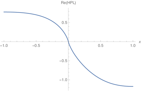
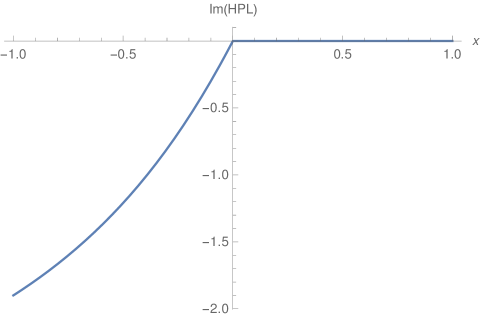
Refer to caption
Refer to caption
Figure 6: The real (left panel) and imaginary part (right panel) of the function H[{6,0},0,x] in the region x[1,1]𝑥11x\in[-1,1].

On the other hand, the former one is limited to double precision, while the latter one can be extended to arbitrary precision. We have tested the numerical implementation of the real-valued cyclotomic HPLs in CPOLY.f comparing to the corresponding results obtained by corresponding numerical results provided by Ginac. The code is compiled by gfortran CPOLY.f. The representation has an accuracy of

21015similar-toabsent2superscript1015\sim 2\cdot 10^{-15} (97)

and better. The reading of the data needed in CPOLY.f requires 5.81025.8superscript1025.8\cdot 10^{-2} sec. The calculation of all 206 cyclotomic HPLs at a given value of x𝑥x is performed in 2.31032.3superscript1032.3\cdot 10^{-3} sec or faster. In using the code CPOLY.f only the subroutines UCPOLYIN and UCPOLY are user routines to provide further input and to perform the calculation, respectively. Any use of the code CPOLY.f requires to quote the present paper.555After completion of this paper another numeric implementation in Mathematica of cyclotomic harmonic polylogarithms appeared in [127].

6 Conclusion

We presented an algorithm to solve single-variate systems of differential equations, factorizing at first order and depending on the dimensional parameter ε𝜀\varepsilon, analytically. Here no choice of a special basis representation is required. The Laurent expansion in the parameter ε𝜀\varepsilon leads to a one-variable problem. We considered differential equations with rational coefficients in x𝑥x and ε𝜀\varepsilon. The algorithm solves these systems in terms of iterative integrals over finite alphabets and rational terms to any order in the dimensional parameter ε𝜀\varepsilon. This method can be applied to a wide range of problems in Quantum Field Theory, after one knows whether the corresponding systems factorize to first order, which is checked by the present algorithm.

In the example of the massive three–loop form factors the emerging letters are those forming the HPLs and the cyclotomic HPLs at cyclotomy c = 3,4 and 6. The homogeneous solutions are the same for any order in ε𝜀\varepsilon. The corresponding inhomogeneities then determine the respective inhomogeneous solutions using the variation of constants. The iterative-integral structure is preserved by the latter operation, as can be shown by integration-by-parts. Besides the harmonic and cyclotomic harmonic polylogarithms up to weight w = 6 also associated special constants appear. In the cyclotomic case not all their relations have been proven yet by analytic methods. However, a series of relations has been conjectured by using PSLQ [78]. Assuming that these relations would hold, the results at three–loop order presented in this paper can finally be expressed by very few multiple zeta values only

{ln(2),ζ2,ζ3,Li4(12),ζ5}2subscript𝜁2subscript𝜁3subscriptLi412subscript𝜁5\left\{\ln(2),\zeta_{2},\zeta_{3},{\rm Li}_{4}\left(\frac{1}{2}\right),\zeta_{5}\right\} (98)

and no special cyclotomic constants contribute. However, cyclotomic constants remain in the expansion around x=1𝑥1x=-1.

Our result for the vector form factors agree with those given in Ref. [49, 50, 51]. We provide the FORTRAN-code CPOLY.f which allows to calculate the cyclotomic harmonic polylogarithms contributing to all massive three-loop form factors in the color–planar limit.

Acknowledgment. We would like to thank M. Round and K. Schönwald for discussions. This work was supported in part by the Austrian Science Fund (FWF) grant SFB F50 (F5009-N15), by the bilateral project DNTS-Austria 01/3/2017 (WTZ BG03/2017), funded by the Bulgarian National Science Fund and OeAD (Austria), by the EU TMR network SAGEX Marie Skłodowska-Curie grant agreement No. 764850 and COST action CA16201: Unraveling new physics at the LHC through the precision frontier. The Feynman diagrams have been drawn using Axodraw [128].

References

  • [1] J. Lagrange, Nouvelles recherches sur la nature et la propagation du son, Miscellanea Taurinensis t. II (1760-61) 263.
  • [2] C.F. Gauß, Theoria attractionis corporum sphaeroidicorum ellipticorum homogeneorum methodo novo tractate, Commentationes societas scientiarum Gottingensis recentiores III (1813) 5–7.
  • [3] G. Green, Essay on the mathematical theory of electricity and magnetism, Nottingham (1828), Green Papers, pp. 1–115.
  • [4] M. Ostrogradski, Mem. Ac. Sci. St. Peters. 6 (1831) 129–133.
  • [5] K.G. Chetyrkin and F.V. Tkachov, Nucl. Phys. B 192 (1981) 159–204.
  • [6] S. Laporta, Int. J. Mod. Phys. A 15 (2000) 5087–5159 [hep-ph/0102033].
  • [7] C. Studerus, Comput. Phys. Commun. 181 (2010) 1293–1300, [arXiv:0912.2546 [physics.comp-ph]];
    A. von Manteuffel and C. Studerus, Reduze 2 - Distributed Feynman Integral Reduction, arXiv:1201.4330 [hep-ph].
  • [8] P. Marquard and D. Seidel, The package Crusher, (unpublished).
  • [9] A.V. Kotikov, Phys. Lett. B254 (1991) 158–164.
  • [10] E. Remiddi, Nuovo Cim. A110 (1997) 1435–1452 [hep-th/9711188].
  • [11] J.M. Henn, Phys. Rev. Lett. 110 (2013) 251601 [arXiv:1304.1806 [hep-th]].
  • [12] J. Ablinger, A. Behring, J. Blümlein, A. De Freitas, A. von Manteuffel and C. Schneider, Comput. Phys. Commun.  202 (2016) 33–112 [arXiv:1509.08324 [hep-ph]].
  • [13] J. Blümlein and C. Schneider, Int. J. Mod. Phys. A 33 (2018) no.17, 1830015.
  • [14] M. Karr, J. ACM 28 (1981) 305–350.
  • [15] M. Bronstein, J. Symbolic Comput. 29 (2000), no. 6 841–877.
  • [16] C. Schneider, Symbolic Summation in Difference Fields, Ph.D. Thesis RISC, Johannes Kepler University, Linz technical report 01–17 (2001).
  • [17] C. Schneider, An. Univ. Timisoara Ser. Mat.-Inform. 42 (2004) 163–179.
  • [18] C. Schneider, J. Differ. Equations Appl. 11 (2005) 799–821.
  • [19] C. Schneider, Appl. Algebra Engrg. Comm. Comput. 16 (2005) 1–32.
  • [20] C. Schneider, J. Algebra Appl. 6 (2007) 415–441.
  • [21] C. Schneider, in: Motives, Quantum Field Theory, and Pseudodifferential Operators, Clay Mathematics Proceedings Vol. 12, eds. A. Carey, D. Ellwood, S. Paycha and S. Rosenberg, (Amer. Math. Soc) (2010), 285–308, [arXiv:0904.2323].
  • [22] C. Schneider, Ann. Comb. 14 (2010) 533–552, [arXiv:0808.2596].
  • [23] C. Schneider, in: Computer Algebra and Polynomials, Applications of Algebra and Number Theory, J. Gutierrez, J. Schicho, M. Weimann (ed.), Lecture Notes in Computer Science (LNCS) 8942 (2015), 157–191, [arXiv:1307.7887 [cs.SC]].
  • [24] C. Schneider, J. Symbolic Comput. 43 (2008) 611–644 [arXiv:0808.2543].
  • [25] C. Schneider, J. Symb. Comput. 72 (2016) 82–127 [arXiv:1408.2776 [cs.SC]].
  • [26] C. Schneider, J. Symb. Comput. 80 (2017) 616–664 [arXiv:1603.04285 [cs.SC]].
  • [27] C. Schneider, Sém. Lothar. Combin. 56 (2007) 1–36, article B56b.
  • [28] C. Schneider, in: Computer Algebra in Quantum Field Theory: Integration, Summation and Special Functions, Texts and Monographs in Symbolic Computation eds. C. Schneider and J. Blümlein (Springer, Wien, 2013), 325–360 [arXiv:1304.4134 [cs.SC]].
  • [29] S. Laporta and E. Remiddi, Nucl. Phys. B704 (2005) 349–386 [hep-ph/0406160].
  • [30] S. Bloch and P. Vanhove, J. Number Theor. 148 (2015) 328–364 [hep-th/1309.5865].
  • [31] L. Adams, C. Bogner, and S. Weinzierl, J. Math. Phys. 56 (2015), no. 7 072303 [hep-ph/1504.03255].
  • [32] L. Adams, C. Bogner, and S. Weinzierl, J. Math. Phys. 55 (2014), no. 10 102301 [hep-ph/1405.5640].
  • [33] L. Adams, C. Bogner, A. Schweitzer, and S. Weinzierl, J. Math. Phys. 57 (2016), no. 12 122302 [hep-ph/1607.01571].
  • [34] J. Ablinger, J. Blümlein, A. De Freitas, M. van Hoeij, E. Imamoglu, C.G. Raab, C.S. Radu and C. Schneider, J. Math. Phys.  59 (2018) no.6, 062305 [arXiv:1706.01299 [hep-th]].
  • [35] J. Brödel, C. Duhr, F. Dulat and L. Tancredi, JHEP 05 (2018) 093 [arXiv:1712.07089 [hep-th]].
  • [36] J. Brödel, C. Duhr, F. Dulat, B. Penante and L. Tancredi, arXiv:1807.00842 [hep-th].
  • [37] Elliptic Integrals, Elliptic Functions and Modular Forms in Quantum Field Theory, Eds. J. Blümlein, P. Paule and C. Schneider, (Springer, Wien, 2018).
  • [38] J. Blümlein, Talk at the 5th International Congress on Mathematical Software ZIB Berlin from July 11 to July 14, 2016, Session: Symbolic computation and elementary particle physics, https://www.risc.jku.at/conferences/ICMS2016/;
    see also talk at QCD@LHC2016, U. Zürich, August 22 to August 26, 2016, https://indico.cern.ch/event/516210/timetable/#all.detailed.
  • [39] F. Abe et al. [CDF Collaboration], Phys. Rev. Lett.  74 (1995) 2626–2631 [hep-ex/9503002].
  • [40] S. Abachi et al. [D0 Collaboration], Phys. Rev. Lett.  74 (1995) 2632–2637 [hep-ex/9503003].
  • [41] https://home.cern/topics/high-luminosity-lhc
  • [42] E. Accomando et al. [ECFA/DESY LC Physics Working Group], Phys. Rept.  299 (1998) 1 [hep-ph/9705442].
  • [43] W. Bernreuther, R. Bonciani, T. Gehrmann, R. Heinesch, T. Leineweber, P. Mastrolia, and E. Remiddi, Nucl. Phys. B706 (2005) 245–324 [hep-ph/0406046].
  • [44] W. Bernreuther, R. Bonciani, T. Gehrmann, R. Heinesch, T. Leineweber, P. Mastrolia, and E. Remiddi, Nucl. Phys. B712 (2005) 229–286 [hep-ph/0412259].
  • [45] W. Bernreuther, R. Bonciani, T. Gehrmann, R. Heinesch, T. Leineweber, and E. Remiddi, Nucl. Phys. B723 (2005) 91–116 [hep-ph/0504190].
  • [46] W. Bernreuther, R. Bonciani, T. Gehrmann, R. Heinesch, P. Mastrolia, and E. Remiddi, Phys. Rev. D72 (2005) 096002 [hep-ph/0508254].
  • [47] J. Gluza, A. Mitov, S. Moch, and T. Riemann, JHEP 07 (2009) 001 [arXiv:0905.1137 [hep-ph]].
  • [48] J. Ablinger, A. Behring, J. Blümlein, G. Falcioni, A. De Freitas, P. Marquard, N. Rana and C. Schneider, Phys. Rev. D 97 (2018) no.9, 094022 [arXiv:1712.09889 [hep-ph]].
  • [49] J.M. Henn, A.V. Smirnov, and V.A. Smirnov, JHEP 12 (2016) 144 [arXiv:1611.06523 [hep-ph]].
  • [50] J.M. Henn, A.V. Smirnov, V.A. Smirnov, and M. Steinhauser, JHEP 01 (2017) 074 [arXiv:1611.07535 [hep-ph]].
  • [51] R.N. Lee, A.V. Smirnov, V.A. Smirnov and M. Steinhauser, JHEP 03 (2018) 136 [arXiv:1801.08151 [hep-ph]].
  • [52] J. Ablinger, J. Blümlein, P. Marquard, N. Rana and C. Schneider, Phys. Lett. B 782 (2018) 528–532 [arXiv:1804.07313 [hep-ph]].
  • [53] R.N. Lee, A.V. Smirnov, V.A. Smirnov and M. Steinhauser, JHEP 05 (2018) 187 [arXiv:1804.07310 [hep-ph]].
  • [54] J. Blümlein, P. Marquard and N. Rana, The asymptotic behavior of the heavy quark form factors at higher order, arXiv:1810.08943 [hep-ph].
  • [55] T. Ahmed, J.M. Henn and M. Steinhauser, JHEP 06 (2017) 125 [arXiv:1704.07846 [hep-ph]].
  • [56] A. Grozin, Eur. Phys. J. C 77 (2017) no.7, 453 [arXiv:1704.07968 [hep-ph]].
  • [57] J.P. Archambault and A. Czarnecki, Phys. Rev. D 70 (2004) 074016 [hep-ph/0408021].
  • [58] J. Blümlein, Comput. Phys. Commun.  159 (2004) 19–54 [hep-ph/0311046].
  • [59] B. Zürcher, Rationale Normalformen von pseudo-linearen Abbildungen, Master’s thesis, Mathematik, ETH Zürich (1994).
  • [60] C. Schneider, A. De Freitas and J. Blümlein, PoS (LL2014) 017 [arXiv:1407.2537 [cs.SC]].
  • [61] A. Bostan, F. Chyzak and É. de Panafieu, Proceedings ISSAC’13, 85–92, (ACM, New York, 2013).
  • [62] S. Gerhold, Uncoupling systems of linear Ore operator equations, Master’s thesis, RISC, J. Kepler University, Linz, 2002.
  • [63] J. Blümlein, S. Klein, C. Schneider and F. Stan, J. Symbolic Comput. 47 (2012) 1267–1289 [arXiv:1011.2656 [cs.SC]].
  • [64] C. Schneider, A. De Freitas and J. Blümlein, PoS (LL2014) 017 [arXiv:1407.2537 [cs.SC]].
  • [65] C. Schneider, J. Ablinger, J. Blümlein and A. de Freitas, PoS (RADCOR2015) 060 [arXiv:1601.01856 [cs.SC]].
  • [66] M.F. Singer, J. Symbolic Comput. 11 (1991) 251–273.
  • [67] M. Bronstein, Proceedings of ISSAC 1992, 42–48 (ACM, New York, 1992).
  • [68] M. van Hoeij, J. Symbolic Comput. 24 (1997) 537–561.
  • [69] M. van der Put and M.F. Singer, Galois theory of linear differential equations, Grundlehren der Mathematischen Wissenschaften 328 (Springer, Berlin, 2003).
  • [70] S.A. Abramov and M. Petkovšek, Proceedings of ISSAC’94 (1994) 169–174, (ACM, New York, 1994).
  • [71] E.E. Kummer, Journal für die reine und angewandte Mathematik (Crelle) 21 (1840) 74–90;
    H. Poincaré, Acta Math. 4 (1884) 201–312.
  • [72] J. Ablinger and C. Schneider, Ann. Comb. 22 (2018) 213–244 [arXiv:1510.03692 [cs.SC]].
  • [73] J. Blümlein, D.J. Broadhurst and J.A.M. Vermaseren, Comput. Phys. Commun.  181 (2010) 582–625 [arXiv:0907.2557 [math-ph]].
  • [74] D.J. Broadhurst, Eur. Phys. J. C 8 (1999) 311 [hep-th/9803091].
  • [75] M.Y. Kalmykov and B.A. Kniehl, Nucl. Phys. Proc. Suppl.  205-206 (2010) 129–134 [arXiv:1007.2373 [math-ph]].
  • [76] J. Ablinger, J. Blümlein, M. Round and C. Schneider, PoS (RADCOR 2017) 010 [arXiv:1712.08541 [hep-th]].
  • [77] J. Ablinger, J. Blümlein, and C. Schneider, J. Math. Phys. 52 (2011) 102301, [arXiv:1105.6063 [math-ph]].
  • [78] J.M. Henn, A.V. Smirnov and V.A. Smirnov, Nucl. Phys. B 919 (2017) 315–324 [arXiv:1512.08389 [hep-th]].
  • [79] H.R.P. Ferguson and D.H. Bailey, A Polynomial Time, Numerically Stable Integer Relation Algorithm, RNR Techn. Rept, RNR-91-032, Jul. 14, 1992.
  • [80] G. Almkvist and D. Zeilberger, J. Symb. Comp. 10 (1990) 571–591;
    M. Apagodu and D. Zeilberger, Adv. Appl. Math. (Special Regev Issue) 37 (2006) 139–152.
  • [81] E. Remiddi and J.A.M. Vermaseren, Int. J. Mod. Phys. A15 (2000) 725–754, [hep-ph/9905237].
  • [82] J.A.M. Vermaseren, Int. J. Mod. Phys. A 14 (1999) 2037–2076 [hep-ph/9806280].
  • [83] J. Blümlein and S. Kurth, Phys. Rev. D 60 (1999) 014018 [hep-ph/9810241].
  • [84] J. Ablinger, J. Blümlein, M. Round and C. Schneider, Numerical Implementation of Harmonic Polylogarithms to Weight w = 8, arXiv:1809.07084 [hep-ph].
  • [85] https://www3.risc.jku.at/research/combinat/software/HarmonicSums/
  • [86] R. Barbieri, J. A. Mignaco, and E. Remiddi, Nuovo Cim. A11 (1972) 824–864; 865–916.
  • [87] P. Nogueira, J. Comput. Phys. 105 (1993) 279–289.
  • [88] T. van Ritbergen, A.N. Schellekens and J.A.M. Vermaseren, Int. J. Mod. Phys. A 14 (1999) 41–96 [hep-ph/9802376].
  • [89] R. Harlander, T. Seidensticker, and M. Steinhauser, Phys. Lett. B426 (1998) 125–132, [hep-ph/9712228].
  • [90] T. Seidensticker, in: Proc. of the 6th International Workshop on New Computing Techniques in Physics Research (AIHENP 99) Heraklion, Crete, Greece, April 12-16, 1999, hep-ph/9905298.
  • [91] J.A.M. Vermaseren, New features of FORM, math-ph/0010025.
  • [92] M. Tentyukov and J.A.M. Vermaseren, Comput. Phys. Commun. 181 (2010) 1419–1427 [hep-ph/0702279].
  • [93] J. Ablinger, PoS (LL2014) 019, [arXiv:1407.6180 [cs.SC]].
  • [94] J. Ablinger, J. Blümlein and C. Schneider, J. Math. Phys.  54 (2013) 082301 [arXiv:1302.0378 [math-ph]].
  • [95] J. Ablinger, A Computer Algebra Toolbox for Harmonic Sums Related to Particle Physics. Master thesis, Linz U., 2009. arXiv:1011.1176 [math-ph].
  • [96] J. Ablinger, Computer Algebra Algorithms for Special Functions in Particle Physics. PhD thesis, Linz U., 2012. arXiv:1305.0687 [math-ph].
  • [97] J. Ablinger, J. Blümlein, C.G. Raab, and C. Schneider, J. Math. Phys. 55 (2014) 112301 [arXiv:1407.1822 [hep-th]].
  • [98] A.V. Smirnov and M.N. Tentyukov, Comput. Phys. Commun.  180 (2009) 735–746 [arXiv:0807.4129 [hep-ph]].
  • [99] A.V. Smirnov, V.A. Smirnov and M. Tentyukov, Comput. Phys. Commun.  182 (2011) 790–803 [arXiv:0912.0158 [hep-ph]].
  • [100] A.V. Smirnov, Comput. Phys. Commun.  204 (2016) 189–199 [arXiv:1511.03614 [hep-ph]].
  • [101] D.J. Broadhurst, N. Gray, and K. Schilcher, Z. Phys. C52 (1991) 111–122.
  • [102] K. Melnikov and T. van Ritbergen, Nucl. Phys. B591 (2000) 515–546 [hep-ph/0005131].
  • [103] P. Marquard, L. Mihaila, J.H. Piclum, and M. Steinhauser, Nucl. Phys. B773 (2007) 1–18 [arXiv:hep-ph/0702185 [hep-ph]].
  • [104] P. Marquard, A.V. Smirnov, V.A. Smirnov and M. Steinhauser, Phys. Rev. Lett.  114 (2015) no.14, 142002 [arXiv:1502.01030 [hep-ph]].
  • [105] P. Marquard, A.V. Smirnov, V.A. Smirnov, M. Steinhauser and D. Wellmann, Phys. Rev. D 94 (2016) no.7, 074025 [arXiv:1606.06754 [hep-ph]].
  • [106] P. Marquard, A.V. Smirnov, V.A. Smirnov and M. Steinhauser, Phys. Rev. D 97 (2018) no.5, 054032 [arXiv:1801.08292 [hep-ph]].
  • [107] O.V. Tarasov, A.A. Vladimirov and A.Y. Zharkov, Phys. Lett.  93B (1980) 429–432
  • [108] S.A. Larin and J.A.M. Vermaseren, Phys. Lett. B 303 (1993) 334–336 [hep-ph/9302208].
  • [109] T. van Ritbergen, J.A.M. Vermaseren and S.A. Larin, Phys. Lett. B 400 (1997) 379–384 [hep-ph/9701390].
  • [110] M. Czakon, Nucl. Phys. B 710 (2005) 485–498 [hep-ph/0411261].
  • [111] P.A. Baikov, K.G. Chetyrkin and J.H. Kühn, Phys. Rev. Lett.  118 (2017) no.8, 082002 [arXiv:1606.08659 [hep-ph]].
  • [112] F. Herzog, B. Ruijl, T. Ueda, J.A.M. Vermaseren and A. Vogt, JHEP 02 (2017) 090 [arXiv:1701.01404 [hep-ph]].
  • [113] T. Luthe, A. Maier, P. Marquard and Y. Schröder, JHEP 10 (2017) 166 [arXiv:1709.07718 [hep-ph]].
  • [114] A. Mitov and S. Moch, JHEP 05 (2007) 001 [hep-ph/0612149].
  • [115] T. Becher and M. Neubert, Phys. Rev. D 79 (2009) 125004 Erratum: [Phys. Rev. D 80 (2009) 109901] [arXiv:0904.1021 [hep-ph]].
  • [116] A. Grozin, J.M. Henn, G.P. Korchemsky, and P. Marquard, Phys. Rev. Lett. 114 no. 6, (2015) 062006, [arXiv:1409.0023 [hep-ph]].
  • [117] A. Grozin, J.M. Henn, G.P. Korchemsky, and P. Marquard, JHEP 01 (2016) 140, [arXiv:1510.07803 [hep-ph]].
  • [118] A. Devoto A and D.W. Duke, Riv. Nuovo Cim.  7N6 (1984) 1–39.
  • [119] L. Lewin, Dilogarithms and associated functions, (Macdonald, London, 1958);
    L. Lewin, Polylogarithms and associated functions, (North Holland, New York, 1981).
  • [120] J. Vollinga and S. Weinzierl, Comput. Phys. Commun.  167 (2005) 177–194 [hep-ph/0410259].
  • [121] C.W. Bauer, A. Frink and R. Kreckel, J. Symb. Comput.  33 (2000) 1–12 [cs/0004015 [cs-sc]].
  • [122] A.G. Grozin, P. Marquard, J.H. Piclum and M. Steinhauser, Nucl. Phys. B 789 (2008) 277–293 [arXiv:0707.1388 [hep-ph]].
  • [123] J. Ablinger, J. Blümlein, C. Raab, C. Schneider and F. Wißbrock, Nucl. Phys. B 885 (2014) 409–447 [arXiv:1403.1137 [hep-ph]].
  • [124] T. Clausen, Journal für die reine und angewandte Mathematik (Crelle) 8 (1832) 298–300.
  • [125] See https://www.ttp.kit.edu/preprints/2018/ttp18-015.
  • [126] T. Gehrmann and E. Remiddi, Comput. Phys. Commun.  141 (2001) 296–312 [hep-ph/0107173].
  • [127] B.A. Kniehl, A.F. Pikelner, and O.L. Veretin, arXiv:1810.07476 [hep-th].
  • [128] J.A.M. Vermaseren, Comput. Phys. Commun.  83 (1994) 45–58.