Prediction of Discretization of GMsFEM using Deep Learning

Abstract

In this paper, we propose a deep-learning-based approach to a class of multiscale problems. THe Generalized Multiscale Finite Element Method (GMsFEM) has been proven successful as a model reduction technique of flow problems in heterogeneous and high-contrast porous media. The key ingredients of GMsFEM include mutlsicale basis functions and coarse-scale parameters, which are obtained from solving local problems in each coarse neighborhood. Given a fixed medium, these quantities are precomputed by solving local problems in an offline stage, and result in a reduced-order model. However, these quantities have to be re-computed in case of varying media. The objective of our work is to make use of deep learning techniques to mimic the nonlinear relation between the permeability field and the GMsFEM discretizations, and use neural networks to perform fast computation of GMsFEM ingredients repeatedly for a class of media. We provide numerical experiments to investigate the predictive power of neural networks and the usefulness of the resultant multiscale model in solving channelized porous media flow problems.

1 Introduction

Multiscale features widely exist in many engineering problems. For instance, in porous media flow, the media properties typically vary over many scales and contain high contrast. Multiscale Finite Element Methods (MsFEM) [14, 21, 22] and Generalized Multiscale Finite Element Methods (GMsFEM) [12, 8] are designed for solving multiscale problems using local model reduction techniques. In these methods, the computational domain is partitioned into a coarse grid $\mathcal{T}^{H}$, which does not necessarily resolve all multiscale features. We further perform a refinement of $\mathcal{T}^{H}$ to obtain a fine grid $\mathcal{T}^{h}$, which essentially resolves all multiscale features. The idea of local model reduction in these methods is based on idenfications of local multiscale basis functions supported in coarse regions on the fine grid, and replacement of the macroscopic equations by a coarse-scale system using a limited number of local multiscale basis functions. As in many model reduction techniques, the computations of multiscale basis functions, which constitute a small dimensional subspace, can be performed in an offline stage. For a fixed medium, these multiscale basis functions are reusable for any force terms and boundary conditions. Therefore, these methods provide a substantial computational savings in the online stage, in which a coarse-scale system is constructed and solved on the reduced-order space.

However, difficulties arise in situations with uncertainties in the media properties in some local regions, which are common for oil reservoirs or aquifers. One straightforward approach for quantifying the uncertainties is to sample realizations of media properties. In such cases, it is challenging to find an offline principal component subspace which is able to universally solve the multiscale problems with different media properties. The computation of multiscale basis functions has to be performed in an online procedure for each medium. Even though the multiscale basis functions are reusable for different force terms and boundary conditions, the computational effort can grow very huge for a large number of realizations of media properties. To this end, building a functional relationship between the media properties and the multiscale model in an offline stage can avoid repeating expensive computations and thus vastly reduce the computational complexity. Due to the diversity of complexity of the media properties, the functional relationship is highly nonlinear. Modelling such a nonlinear functional relationship typically involves high-order approximations. Therefore, it is natural to use machine learning techniques to devise such complex models. In [15, 3], the authors make use of a Bayesian approach for learning multiscale models and incorporating essential observation data in the presence of uncertainties.

Deep neural networks is one class of machine learning algorithm that is based on an artificial neural network, which is composed of a relatively large number of layers of nonlinear processing units, called neurons, for feature extraction. The neurons are connected to other neurons in the successive layers. The information propagates from the input, through the intermediate hidden layers, and to the output layer. In the propagation process, the output in each layer is used as input in the consecutive layer. Each layer transforms its input data into a little more abstract feature representation. In between layers, a nonlinear activation function is used as the nonlinear transformation on the input, which increases the expressive power of neural networks. Recently, deep neural network (DNN) has been successfully used to interpret complicated data sets and applied to tasks with pattern recognition, such as image recognition, speech recognition and natural language processing [25, 19, 18]. Extensive researches have also been conducted on investigating the expression power of deep neural networks [11, 20, 10, 28, 27, 17]. Results show that neural networks can represent and approximate a large class of functions. Recently, deep learning has been applied to model reductions and partial differential equations. In [31], the authors studied deep convolution networks for surrogate model construction. on dynamic flow problems in heterogeneous media. In [26], the authors studied the relationship between residual networks (ResNet) and characteristic equations of linear transport, and proposed an interpretation of deep neural networks by continuous flow models. In [30], the authors combined the idea of the Ritz method and deep learning techniques to solve elliptic problems and eigenvalue problems. In [23], a neural network has been designed to learn the physical quantities of interest as a function of random input coefficients. The concept of using deep learning to generate a reduced-order model for a dynamic flow has been applied to proper orthogonal decomposition (POD) global model reduction [2] and nonlocal multi-continuum upscaling (NLMC) [29].

In this work, we propose a deep-learning-based method for fast computation of the GMsFEM discretization. Our approach makes use of deep neural networks as a fast proxy to compute GMsFEM discretizations for flow problems in channelized porous media with uncertainties. More specifically, neural networks are used to express the functional relationship between the media properties and the multiscale model. Such networks are built up in an offline stage. Sufficient sample pairs are required to ensure the expressive power of the networks. With different realizations of media properties, one can use the built network and avoid computations of local problems and spectral problems.

The paper is organized as follows. We start with the underlying partial differential equation that describes the flow within a heterogeneous media and the main ingredients of GMsFEM in Section 2. Next, in Section 3, we present the idea of using deep learning as a proxy for prediction of GMsFEM discretizations. The networks will be precisely defined and the sampling will be explained in detail. In Section 4, we present numerical experiments to show the effectiveness of our presented networks on several examples with different configurations. Finally, a conclusive discussion is provided in Section 5.

2 Preliminaries

In this paper, we are considering the flow problem in highly heterogeneous media

$$\begin{split}-\text{div}\big{(}\kappa\,\nabla u\big{)}=f\quad&\text{in}\quad\Omega,\\ u=0\quad\text{or}\quad\frac{\partial u}{\partial n}=0\quad&\text{on}\quad\partial\Omega,\end{split}$$ (1)

where $\Omega$ is the computational domain, $\kappa$ is the permeability coefficient in $L^{\infty}(\Omega)$, and $f$ is a source function in $L^{2}(\Omega)$. We assume the coefficient $\kappa$ is highly heterogeneous with high contrast. The classical finite element method for solving (1) numerically is given by: find $u_{h}\in V_{h}$ such that

$$\begin{split}a(u_{h},v)=\int_{\Omega}\kappa\nabla u_{h}\cdot\nabla v~{}dx&=\int_{\Omega}fv~{}dx=(f,v)\quad\text{for all}\,\,v\in V_{h},\\ \end{split}$$ (2)

where $V_{h}$ is a standard conforming finite element space over a partition $\mathcal{T}_{h}$ of $\Omega$ with mesh size $h$.

However, with the highly heterougeneous property of coefficient $\kappa$, the mesh size $h$ has to be taken extremely small to capture the underlying fine-scale features of $\kappa$. This ends up with a large computational cost. Generalized Multiscale Finite Element Method (GMsFEM) [12, 8] serves as a model reduction technique to reduce the number of degree of freedom and attain both efficiency and accuracy to a considerable extent. GMsFEM has been successfully extended to other formulations and applied to other problems. Here we provide a brief introduction of the main ingredients of GMsFEM. For a more detailed discussion of GMsFEM and related concepts, the reader is referred to [6, 5, 13, 1, 7].

In GMsFEM, we define a coarse mesh $\mathcal{T}^{H}$ over the domain $\Omega$ and refine to obtain a fine mesh $\mathcal{T}^{h}$ with mesh size $h\ll H$, which is fine enough to restore the multiscale properties of the problem. Multiscale basis functions are defined on coarse grid blocks using linear combinations of finite element basis functions on $\mathcal{T}^{h}$, and designed to resolve the local multiscale behaviors of the exact solution. The multiscale finite element space $V_{\text{ms}}$, which is a principal component subspace of the conforming finite space $V_{h}$ with $\text{dim}(V_{\text{ms}})\ll\text{dim}(V_{h})$, is constructed by the linear span of multiscale basis functions. The multiscale solution $u_{\text{ms}}\in V_{\text{ms}}$ is then defined by

$$a(u_{\text{ms}},v)=(f,v)\quad\text{for all}\,\,v\in V_{\text{ms}}.$$ (3)

In this work, we consider the identification of dominant modes for solving (1) by multiscale basis functions, including spectral basis functions and simplified basis functions, in GMsFEM. Here, we present the details of the construction of multiscale basis functions in GMsFEM. Let $N_{x}=\{x_{i}\;|1\leq i\leq N_{v}\}$ be the set of nodes of the coarse mesh $\mathcal{T}^{H}$. For each coarse grid node $x_{i}\in N_{x}$, the coarse neighborhood $\omega_{i}$ is defined by

$$\omega_{i}=\bigcup\{K_{j}\in\mathcal{T}^{H};~{}~{}~{}x_{i}\in\overline{K}_{j}\},$$ (4)

that is, the union of the coarse elements $K_{j}\in\mathcal{T}^{H}$ containing the coarse grid node $x_{i}$. An example of the coarse and fine mesh, coarse blocks and a coarse neighborhood is shown in Figure 1. For each coarse neighbourhood $\omega_{i}$, we construct multiscale basis functions $\{\phi_{j}^{\omega_{i}}\}_{j=1}^{L_{i}}$ supported on $\omega_{i}$.

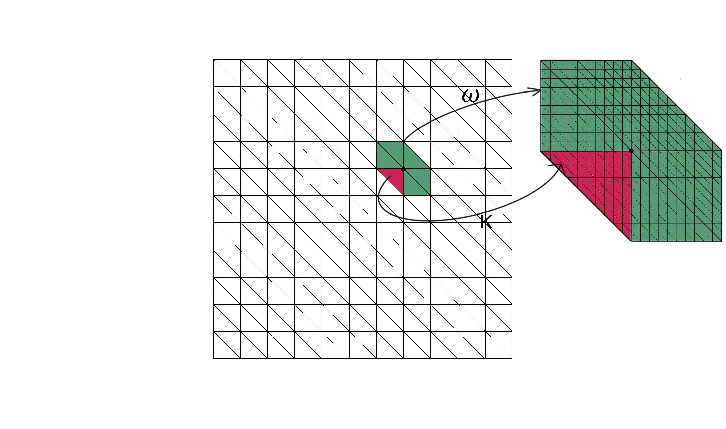
Figure 1: An illustration of coarse mesh (left), a coarse neighborhood and coarse blocks (right)

For the construction of spectral basis functions, we first construct a snapshot space $V_{\text{snap}}^{(i)}$ spanned by local snapshot basis functions $\psi_{\text{snap}}^{i,k}$ for each local coarse neighborhood $\omega_{i}$. The snapshot basis function $\psi_{\text{snap}}^{i,k}$ is the solution of a local problem

$$\begin{split}-\text{div}(\kappa\nabla\psi_{\text{snap}}^{i,k})=0,&\quad\text{in}\quad\omega_{i}\\ \psi_{\text{snap}}^{i,k}=\delta_{i,k},&\quad\text{on}\quad\partial\omega_{i}\end{split}$$ (5)

The fine grid functions $\delta_{i,k}$ is a function defined for all $x_{s}\in\partial\omega_{i}$, where $\{x_{s}\}$ denote the fine degrees of freedom on the boundary of local coarse region $\omega_{i}$. In specific,

$$\delta_{i,k}(x_{s})=\begin{cases}1&\text{if $s=k$}\\ 0&\text{if $s\neq k$}\end{cases}$$

The linear span of these harmonic extensions forms the local snapshot space $V_{\text{snap}}^{(i)}=\text{span}_{k}\{\psi_{\text{snap}}^{i,k}\}$. One can also use randomized boundary conditions to reduce the computational cost associated with snapshot calculations [1]. Next, a spectral problem is designed based on our analysis and used to reduce the dimension of local multiscale space. More precisely, we seek for eigenvalues $\lambda_{m}^{i}$ and corresponding eigenfunctions $\phi^{\omega_{i}}_{m}\in V_{\text{snap}}^{(i)}$ satisfying

$$a_{i}(\phi^{\omega_{i}}_{m},v)=\lambda_{m}^{i}s_{i}(\phi^{\omega_{i}}_{m},v),\quad\forall v\in V_{\text{snap}}^{(i)},$$ (6)

where the bilinear forms in the spectral problem are defined as

$$\begin{split}a_{i}(u,v)&=\int_{\omega_{i}}\kappa\nabla u\cdot\nabla v,\\ s_{i}(u,v)&=\int_{\omega_{i}}\tilde{\kappa}uv,\end{split}$$ (7)

where $\tilde{\kappa}=\sum_{j}\kappa|\nabla\chi_{j}|^{2}$, and $\chi_{j}$ denotes the multiscale partition of unity function. We arrange the eigenvalues $\lambda_{m}^{i}$ of the spectral problem (6) in ascending order, and select the first $l_{i}$ eigenfunctions $\{\phi^{\omega_{i}}_{m}\}_{m=1}^{l_{i}}$ corresponding to the small eigenvalues as the multiscale basis functions.

An alternative way to construct the multiscale basis function is using the idea of simplified basis functions. This approach assumes the number of channels and position of the channalized permeability field are known. Therefore we can obtain multiscale basis functions $\{\phi_{m}^{\omega_{i}}\}_{m=1}^{l_{i}}$ using these information and without solving the spectral problem [9].

Once the multiscale basis functions are constructed, the span of the multiscale basis functions will form the offline space

$$\begin{split}V_{ms}^{(i)}&=\text{span}\{\phi_{m}^{\omega_{i}}\}_{m=1}^{l_{i}},\\ V_{ms}&=\oplus_{i}V_{ms}^{(i)}.\end{split}$$ (8)

We will then seek a multlscale solution $u_{ms}\in V_{ms}$ satisfying

$$a(u_{ms},v)=(f,v)\quad\text{ for all }v\in V_{ms}.$$ (9)

which is a Galerkin projection of the (1) onto $V_{ms}$, and can be written as a system of linear equations

$$A_{c}u_{c}=b_{c},$$ (10)

where $A_{c}$ and $b_{c}$ are the coarse-scale stiffness matrix and load vector. If we collect all the multiscale basis functions and arrange the fine-scale coordinate representation in columns, we obtain the downscaling operator $R$. Then the fine-scale representation of the multiscale solution is given by

$$u_{ms}=Ru_{c}.$$ (11)

3 Deep Learning for GMsFEM

In real world applications, there are uncertainties within some local regions of the permeability field $\kappa$ in the flow problem. Thousands of forward simulations are needed to quantify the uncertainties of the flow solution. GMsFEM provides us with a fast solver to compute the solutions accurately and efficiently. Considering that there is a large amount of simulation data, we are interested in developing a method utilizing the existing offline data and reducing direct computational effort later. In this work, we aim at using DNN to model the relationship between heterogeneous permeability coefficient $\kappa$ and the key ingredients of GMsFEM solver, i.e., coarse scale stiffness matrices and multiscale basis functions. When the relation is built up, we can feed the network any realization of the permeability field and obtain the corresponding GMsFEM ingredients, and further restore fine-grid GMsFEM solution of (1). The general idea of utilizing deep learning in the GMsFEM framework is illustrated in Figure 2.

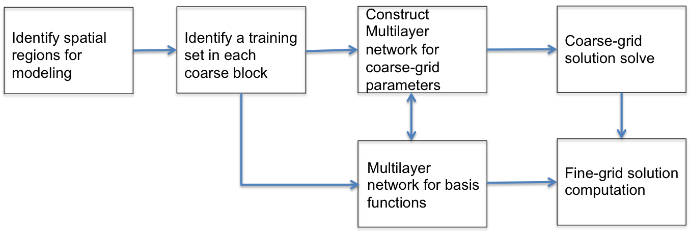
Figure 2: A flow chart in illustrating the idea of using deep learning in the GMsFEM framework.

Suppose that there are uncertainties for the heterogeneous coefficient in a local coarse block $K_{0}$, which we call the target block, and the permeability outside the target block remains the same. For example, for a channelized permeability field, the position, location and the permeability values of the channels in the target block can vary. The target block $K_{0}$ is inside $3$ coarse neighborhoods, denoted by $\omega_{1},\omega_{2},\omega_{3}$. The union of the $3$ neighborhoods, i.e.

$$\omega^{+}(K_{0})=\omega_{1}\cup\omega_{2}\cup\omega_{3},$$

are constituted of by the target block $K_{0}$ and $12$ other coarse blocks, denoted by $\{K_{l}\}_{l=1}^{12}$ A target block and its surrounding neighborhoods are depicted in Figure 3.

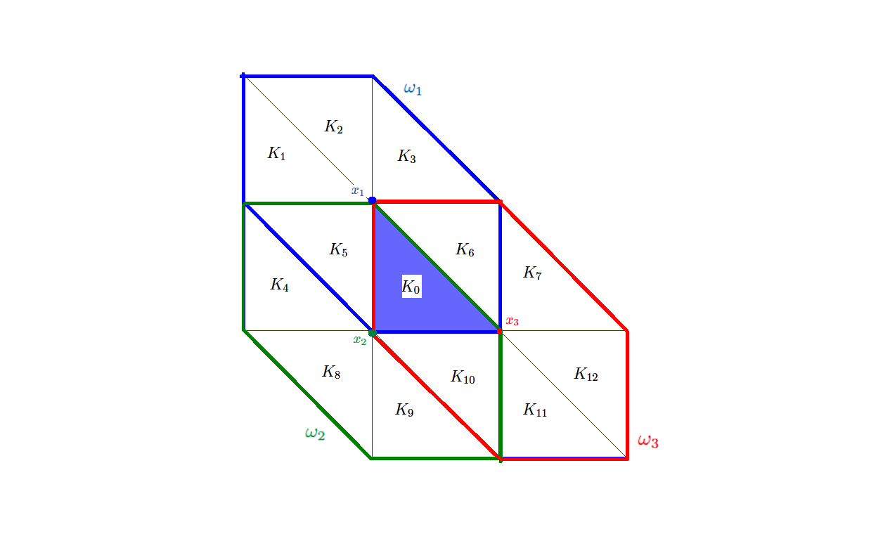
Figure 3: An illustration of a target coarse block $K_{0}$ and related neighborhoods.

For a fixed permeability field $\kappa$, one can compute the multiscale basis functions $\phi_{m}^{\omega_{i}}(\kappa)$ defined by (6), for $i=1,2,3$, and the local coarse-scale stiffness matrices $A_{c}^{K_{l}}(\kappa)$, defined by

$$[A_{c}^{K_{l}}(\kappa)]^{i,j}_{m,n}=\int_{K_{l}}\kappa\nabla\phi_{m}^{\omega_{i}}(\kappa)\cdot\nabla\phi_{n}^{\omega_{j}}(\kappa).$$ (12)

for $l=0,1,\ldots,12$. We are interested in constructing the maps $g_{B}^{m,i}$ and $g_{M}^{l}$, where

• $g_{B}^{m,i}$ maps the permeability coefficient $\kappa$ to a local multiscale basis function $\phi^{\omega_{i}}_{m}$, where $i$ denotes the index of the coarse block, and $m$ denotes the index of the basis in coarse block $\omega_{i}$

  $$g_{B}^{m,i}:\kappa\mapsto\phi_{m}^{\omega_{i}}(\kappa),$$

• $g_{M}^{l}$ maps the permeability coefficient $\kappa$ to the coarse grid parameters $A_{c}^{K_{l}}$ ($l=0,\cdots,12$)

  $$g_{M}^{l}:\kappa\mapsto A_{c}^{K_{l}}(\kappa).$$

In this work, our goal is to make use of deep learning to build fast approximations of these quantities associated with the uncertainties in the permeability field $\kappa$, which can provide fast and accurate solutions to the heterogeneous flow problem (1).

For each realization $\kappa$, one can compute the images of $\kappa$ under the local multiscale basis maps $g_{B}^{m,i}$ and the local coarse-scale matrix maps $g_{M}^{l}$. These forward calculations serve as training samples for building a deep neural network for approximation of the corresponding maps, i.e.

$$\begin{split}\mathcal{N}_{B}^{m,i}(\kappa)&\approx g_{B}^{m,i}(\kappa),\\ \mathcal{N}_{M}^{l}(\kappa)&\approx g_{M}^{l}(\kappa).\end{split}$$ (13)

In our networks, the permeability field $\kappa$ is the input, while the multiscale basis functions $\phi^{\omega_{i}}_{m}$ and the coarse-scale matrix $A_{c}^{K_{l}}$ are the outputs. Once the neural networks are built, we can use the networks to compute the multiscale basis functions and coarse-scale parameters in the associated region for any permeability field $\kappa$. Using these local information from the neural networks together with the global information which can be pre-computed, we can form the downscale operator $R$ with the multiscale basis functions, form and solve the linear system (10), and obtain the multiscale solution by (11).

3.1 Network architecture

In general, a $L$-layer neural network $\mathcal{N}$ can be written in the form

$$\mathcal{N}(x;\theta)=\sigma(W_{L}\sigma(\cdots\sigma(W_{2}\sigma(W_{1}x+b_{1})+b_{2})\cdots)+b_{L}),$$

where $\theta:=(W_{1},W_{2},\cdots,W_{L},b_{1},b_{2},\cdots,b_{L})$, $W$’s are the weight matrices and $b$’s are the bias vectors, $\sigma$ is the activation function, $x$ is the input. Such a network is used to approximate the output $y$. Our goal is then to find $\theta^{*}$ by solving an optimization problem

$$\theta^{*}=\operatorname*{\text{argmin}}_{\theta}~{}~{}\mathcal{L}(\theta),$$

where $\mathcal{L}(\theta)$ is called loss function, which measures the mismatch between the image of the input $x$ under the the neural network $\mathcal{N}(x,y;\theta)$ and the desired output $y$ in a set of training samples $(x_{j},y_{j})$. In this paper, we use the mean-squared error metric to be our loss function

$$\mathcal{L}(\theta)=\frac{1}{N}\sum_{j=1}^{N}\|y_{j}-\mathcal{N}(x_{j};\theta)\|^{2}_{2},$$

where $N$ is the number of the training samples. An illustration of a deep neural network is shown in Figure 4.

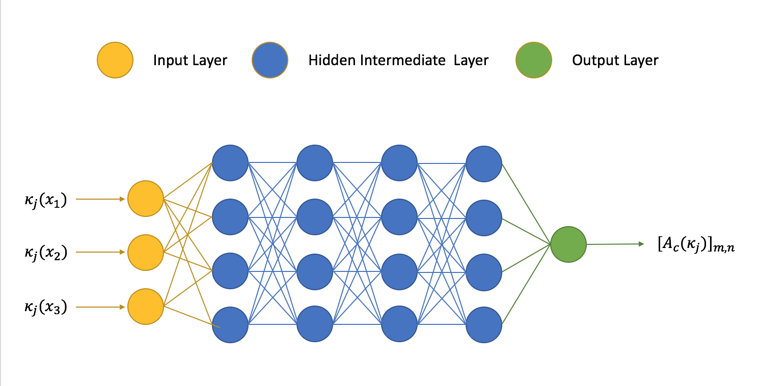
Figure 4: An illustration of a deep neural network.

Suppose we have a set of different realizations of the permeability $\{\kappa_{1},\kappa_{2},\cdots,\kappa_{N}\}$ in the target block. In our network, the input $x_{j}=\kappa_{j}\in\mathbb{R}^{d}$ is a vector containing the permeability image pixels in the target block. The output $y_{j}$ is an entry of the local stiffness matrix $A_{c}^{K_{l}}$, or the coordinate representation of a multiscale basis function $\phi_{m}^{\omega_{i}}$. We will make use of these sample pairs $(x_{j},y_{j})$ to train a deep neural network $\mathcal{N}_{B}^{m,i}(x;\theta_{B}^{*})$ and $\mathcal{N}_{M}^{l}(x;\theta_{M}^{*})$ by minimizing the loss function with respect to the network parameter $\theta$, such that the trained neural networks can approximate the functions $g_{B}^{m,i}$ and $g_{M}^{l}$, respectively. Once the neural is constructed, for some given new permeability coefficient $\kappa_{{N+1}}$, we use our trained networks to compute a fast prediction of the outputs, i.e. local multiscale basis functions $\phi_{m}^{\omega_{i},\text{pred}}$ by

$$\phi_{m}^{\omega_{i},\text{pred}}(\kappa_{N+1})=\mathcal{N}_{B}^{m,i}(\kappa_{{N+1}};\theta_{B}^{*})\approx g_{B}^{m,i}(\kappa_{N+1})=\phi_{m}^{\omega_{i}}(\kappa_{N+1}),$$

and local coarse-scale stiffness matrix $A_{c}^{K_{l},\text{pred}}$ by

$$A_{c}^{K_{l},\text{pred}}(\kappa_{N+1})=\mathcal{N}_{M}^{l}(\kappa_{{N+1}};\theta_{M}^{*})\approx g_{M}^{l}(\kappa_{N+1})=A_{c}^{K_{l}}(\kappa_{N+1}).$$

3.2 Network-based multiscale solver

Once the neural networks are built, we can assemble the predicted multiscale basis functions to obtain a prediction $R^{\text{pred}}$ for the downscaling operator, and assemble the predicted local coarse-scale stiffness matrix $A_{c}^{K_{l},\text{pred}}$ in the global matrix $A_{c}^{\text{pred}}$. Following (10) and (11), we solve the predicted coarse-scale coefficient vector $u_{c}^{\text{pred}}$ from the following linear system

$$A_{c}^{\text{pred}}u_{c}^{\text{pred}}=b_{c},$$ (14)

and obtain the predicted multiscale solution $u_{ms}^{\text{pred}}$ by

$$u_{ms}^{\text{pred}}=R^{\text{pred}}u_{c}^{\text{pred}}.$$ (15)

4 Numerical Results

In this section, we present some numerical results for predicting the GMsFEM ingredients and solutions using our proposed method. We consider permeability fields $\kappa$ with high-contrast channels inside the domain $\Omega=(0,1)^{2}$, which consist of uncertainties in a target cell $K_{0}$. More precisely, we consider a number of random realizations of permeability fields $\kappa_{1},\kappa_{2},\kappa_{3},\cdots,\kappa_{N+M}$. Each permeability field contains two high-conductivity channels, and the fields differ in the target cell $K_{0}$ by:

• in Experiment 1, the channel configurations are all distinct, and the permeability coefficients inside the channels are fixed in each sample (see Figure 5 for illustrations), and

• in Experiment 2, the channel configurations are randomly chosen among 5 configurations, and the permeability coefficients inside the channels follow a random distribution (see Figure 6 for illustrations).

In these numerical experiments, we assume there are uncertainties in only the target block $K_{0}$. The permeability field in $\Omega\setminus K_{0}$ is fixed across all the samples.

We follow the procedures in Section 3 and to generate sample pairs using GMsFEM. Local spectral problems are solved to obtain the multiscale basis functions $\phi_{m}^{\omega_{i}}$. In the neural network, the permeability field $x=\kappa$ is considered to be the input, while the local multiscale basis functions $y=\phi_{m}^{\omega_{i}}$ and local coarse-scale matrices $y=A_{c}^{K_{l}}$ are regarded as the output. These sample pairs are divided into the training set and the learning set in a random manner. A large number $N$ of realizations, namely $\kappa_{1},\kappa_{2},\ldots,\kappa_{N}$, are used to generate sample pairs in the training set, while the remaining $M$ realizations, namely, $\kappa_{N+1},\kappa_{N+2},\ldots,\kappa_{N+M}$ are used in testing the predictive power of the trained network. We remark that, for each basis function and each local matrix, we solve an optimization problem in minimizing the loss function defined by the sample pairs in the training set, and build a separate deep neural network. We summarize the network architectures for training local coarse scale stiffness matrix and multiscale basis functions as below:

• For the multiscale basis function $\phi_{m}^{\omega_{i}}$, we build a network $\mathcal{N}_{B}^{m,i}$ using

  • Input: Vectorized permeability pixels values $\kappa$,

  • Output: Coefficient vector of multiscale basis $\phi_{m}^{\omega_{i}}(\kappa)$ on coarse neighborhood $\omega_{i}$,

  • Loss Function: Mean squared error $\displaystyle\frac{1}{N}\sum_{j=1}^{N}||\phi_{m}^{\omega_{i}}(\kappa_{j})-\mathcal{N}_{B}^{m,i}(\kappa_{j};\theta_{B})||_{2}^{2}$,

  • Activation Function: Leaky ReLu function,

  • DNN structure: 10-20 hidden layers, each layer have 250-350 neurons,

  • Training Optimizer: Adamax.

• For the local coarse scale stiffness matrix $A_{c}^{K_{l}}$, we build a network $\mathcal{N}_{M}^{l}$ using

  • Input: Vectorized permeability pixels values $\kappa$,

  • Output: Vectorized coarse scale stiffness matrix $A_{c}^{K_{l}}(\kappa)$ on the coarse block $K_{l}$,

  • Loss Function: Mean squared error $\displaystyle\frac{1}{N}\sum_{j=1}^{N}||A_{c}^{K_{l}}(\kappa_{j})-\mathcal{N}_{M}^{l}(\kappa_{j};\theta_{M})||_{2}^{2}$,

  • Activation Function: ReLu function (Rectifier),

  • DNN structure: 10-16 hidden layers, each layer have 100-500 neurons,

  • Training Optimizer: Proximal Adagrad.

For simplicity, the activation functions ReLU function [16] and Leaky ReLU function are used as they have the simplest derivatives among all nonlinear functions. The ReLU function is proved to be useful in training deep neural network architectures The Leaky ReLU function can resolve the vanishing gradient problem which can accelerate the training in some occasions. The optimizers Adamax and Proximal Adagrad are stochastic gradient descent (SGD) based methods commonly used in neural network training [24]. In both experiments, we trained our network using Python API Tensorflow and Keras [4].

Once a neural network is built on training, it can be used to predict the output given a new input. The accuracy of the predictions is essential in making the network useful. In our experiments, we use of $M$ sample pairs, which are not used in training the network, to examine the predictive power of our network. On these sample pairs, referred to as the testing set, we compare the prediction and the exact output and compute the mismatch in some suitable metric. Here, we summarize the metric used in our numerical experiment. For the multiscale basis functions, we compute the relative error in $L^{2}$ and $H^{1}$ norm, i.e.

$$\begin{split}e_{L^{2}}(\kappa_{N+j})&=\left(\dfrac{\int_{\Omega}\left|\phi_{m}^{\omega_{i}}(\kappa_{N+j})-\phi_{m}^{\omega_{i},\text{pred}}(\kappa_{N+j})\right|^{2}}{\int_{\Omega}\left|\phi_{m}^{\omega_{i}}(\kappa_{N+j})\right|^{2}}\right)^{\frac{1}{2}},\\ e_{H^{1}}(\kappa_{N+j})&=\left(\dfrac{\int_{\Omega}\left|\nabla\phi_{m}^{\omega_{i}}(\kappa_{N+j})-\nabla\phi_{m}^{\omega_{i},\text{pred}}(\kappa_{N+j})\right|^{2}}{\int_{\Omega}\left|\nabla\phi_{m}^{\omega_{i}}(\kappa_{N+j})\right|^{2}}\right)^{\frac{1}{2}}.\end{split}$$ (16)

For the local stiffness matrices, we compute the relative error in entrywise $\ell^{2}$, entrywise $\ell^{\infty}$ and Frobenius norm, i.e.

$$\begin{split}e_{\ell^{2}}(\kappa_{N+j})&=\dfrac{\|A_{c}^{K_{l}}(\kappa_{N+j})-A_{c}^{K_{l},\text{pred}}(\kappa_{N+j})\|_{2}}{\|A_{c}^{K_{l}}(\kappa_{N+j})\|_{2}},\\ e_{\ell^{\infty}}(\kappa_{N+j})&=\dfrac{\|A_{c}^{K_{l}}(\kappa_{N+j})-A_{c}^{K_{l},\text{pred}}(\kappa_{N+j})\|_{\infty}}{\|A_{c}^{K_{l}}(\kappa_{N+j})\|_{\infty}},\\ e_{F}(\kappa_{N+j})&=\dfrac{\|A_{c}^{K_{l}}(\kappa_{N+j})-A_{c}^{K_{l},\text{pred}}(\kappa_{N+j})\|_{F}}{\|A_{c}^{K_{l}}(\kappa_{N+j})\|_{F}}.\end{split}$$ (17)

A more important measure of the usefulness of the trained neural network is the predicted multiscale solution $u_{ms}^{\text{pred}}(\kappa)$ given by (14)–(15). We compare the predicted solution to $u_{ms}$ defined by (10)–(11), and compute the relative error in $L^{2}$ and energy norm, i.e.

$$\begin{split}e_{L^{2}}(\kappa_{N+j})&=\left(\dfrac{\int_{\Omega}\left|u_{ms}(\kappa_{N+j})-u_{ms}^{\text{pred}}(\kappa_{N+j})\right|^{2}}{\int_{\Omega}\left|u_{ms}(\kappa_{N+j})\right|^{2}}\right)^{\frac{1}{2}},\\ e_{a}(\kappa_{N+j})&=\left(\dfrac{\int_{\Omega}\kappa_{j}\left|\nabla u_{ms}(\kappa_{N+j})-\nabla u_{ms}^{\text{pred}}(\kappa_{N+j})\right|^{2}}{\int_{\Omega}\kappa_{j}\left|\nabla u_{ms}(\kappa_{N+j})\right|^{2}}\right)^{\frac{1}{2}}.\end{split}$$ (18)

4.1 Experiment 1

In this experiment, we consider curved channelized permeability fields. Each permeability field contains a straight channel and a curved channel. The straight channel is fixed and the curved channel strikes the boundary of the target cell $K_{0}$ at the same points. The curvature of the sine-shaped channel inside $K_{0}$ varies among all realizations. We generate 2000 realizations of permeability fields, where the permeability coefficients are fixed. Samples of permeability fields are depicted in Figure 5. Among the 2000 realizations, 1980 sample pairs are randomly chosen and used as training samples, and the remaining 20 sample pairs are used as testing samples.

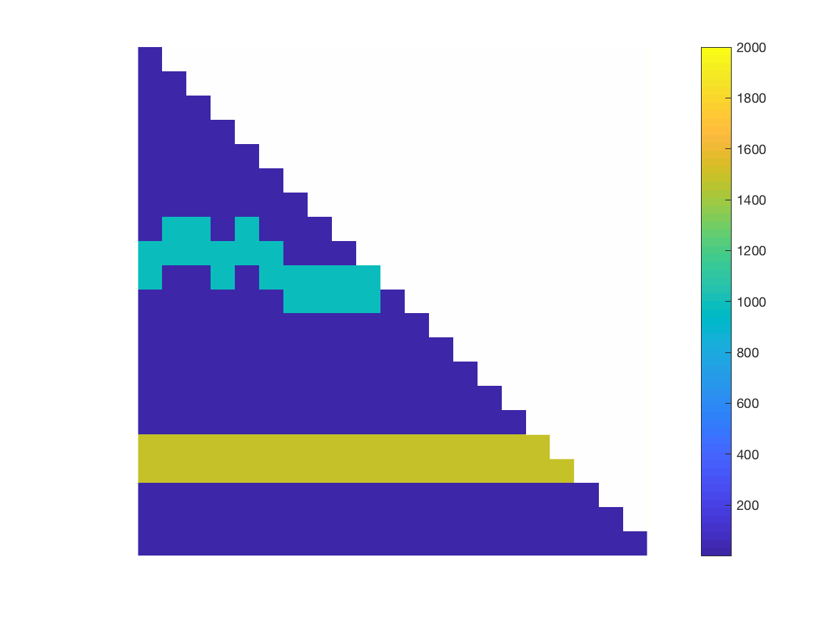
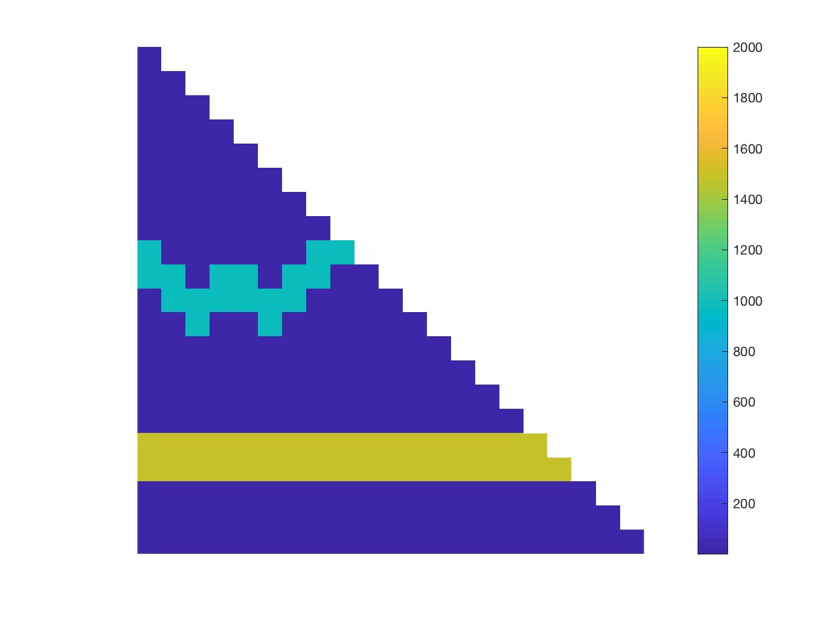
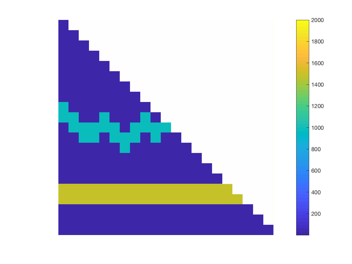
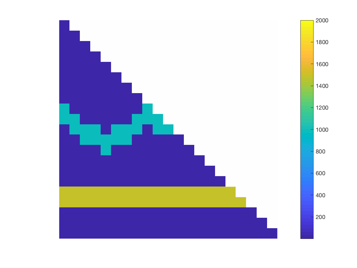
Figure 5: Samples of permeability fields in the target block $K_{0}$ in Experiment 1.

For each realization, we compute the local multiscale basis functions and local coarse-scale stiffness matrix. In building the local snapshot space, we solve for harmonic extension of all the fine-grid boundary conditions. Local multiscale basis functions are then constructed by solving the spectral problem and multiplied the spectral basis functions with the multiscale partition of unity functions. With the offline space constructed, we compute the coarse-scale stiffness matrix. We use the training samples to build deep neural networks for approximating these GMsFEM quantities, and examine the performance of the approximations on the testing set.

Tables 1–3 record the error of the prediction by the neural networks in each testing sample and the mean error measured in the defined metric. It can be seen that the prediction are of high accuracy. This is vital in ensuring the predicted GMsFEM solver useful. Table 4 records the error of the multiscale solution in each testing sample and the mean error using our proposed method. It can be observed that using the predicted GMsFEM solver, we obtain a good approximation of the multiscale solution compared with the exact GMsFEM solver.

Sample	$\omega_{1}$		$\omega_{2}$		$\omega_{3}$
$j$	$e_{L^{2}}$	$e_{H^{1}}$	$e_{L^{2}}$	$e_{H^{1}}$	$e_{L^{2}}$	$e_{H^{1}}$
1	0.47%	3.2%	0.40%	3.6%	0.84%	5.1%
2	0.45%	4.4%	0.39%	3.3%	1.00%	6.3%
3	0.34%	2.3%	0.40%	3.1%	0.88%	4.3%
4	0.35%	4.2%	0.43%	5.4%	0.94%	6.6%
5	0.35%	3.3%	0.37%	3.9%	0.90%	6.1%
6	0.51%	4.7%	0.92%	12.0%	2.60%	19.0%
7	0.45%	4.1%	0.38%	3.2%	1.00%	6.4%
8	0.31%	3.4%	0.43%	5.5%	1.10%	7.7%
9	0.25%	2.2%	0.46%	5.6%	1.10%	6.2%
10	0.31%	3.5%	0.42%	4.5%	1.30%	7.6%
Mean	0.38%	3.5%	0.46%	5.0%	1.17%	7.5%

Table 1: Percentage error of multiscale basis functions $\phi_{1}^{\omega_{i}}$ in Experiment 1.

Sample	$\omega_{1}$		$\omega_{2}$		$\omega_{3}$
$j$	$e_{L^{2}}$	$e_{H^{1}}$	$e_{L^{2}}$	$e_{H^{1}}$	$e_{L^{2}}$	$e_{H^{1}}$
1	0.47%	4.2%	0.40%	1.4%	0.32%	1.1%
2	0.57%	3.2%	0.31%	1.4%	0.30%	1.1%
3	0.58%	2.7%	0.31%	1.4%	0.33%	1.1%
4	0.59%	3.6%	0.13%	1.3%	0.32%	1.1%
5	0.53%	4.0%	0.51%	1.6%	0.27%	1.0%
6	0.85%	4.3%	0.51%	2.1%	0.29%	1.3%
7	0.50%	2.7%	0.22%	1.5%	0.29%	1.0%
8	0.43%	4.5%	0.61%	1.9%	0.35%	1.1%
9	0.71%	2.9%	0.14%	1.4%	0.27%	1.1%
10	0.66%	4.4%	0.53%	1.8%	0.26%	1.1%
Mean	0.59%	3.6%	0.37%	1.6%	0.30%	1.1%

Table 2: Percentage error of multiscale basis functions $\phi_{2}^{\omega_{i}}$ in Experiment 1.

Sample $j$	$e_{\ell^{2}}$	$e_{F}$
1	0.67%	0.84%
2	0.37%	0.37%
3	0.32%	0.38%
4	1.32%	1.29%
5	0.51%	0.59%
6	4.43%	4.28%
7	0.34%	0.38%
8	0.86%	1.04%
9	1.00%	0.97%
10	0.90%	1.08%
Mean	0.76%	0.81%

Table 3: Percentage error of the local stiffness matrix $A_{c}^{K_{0}}$ in Experiment 1.

Sample $j$	$e_{L^{2}}$	$e_{a}$
1	0.31%	4.58%
2	0.30%	4.60%
3	0.30%	4.51%
4	0.27%	4.60%
5	0.29%	4.56%
6	0.47%	4.67%
7	0.39%	4.70%
8	0.30%	4.63%
9	0.35%	4.65%
10	0.31%	4.65%
Mean	0.33%	4.62%

Table 4: Percentage error of multiscale solution $u_{ms}$ in Experiment 1.

4.2 Experiment 2

In this experiment, we consider sine-shaped channelized permeability fields. Each permeability field contains a straight channel and a sine-shaped channel. There are altogether 5 channel configurations, where the straight channel is fixed and the sine-shaped channel strikes the boundary of the target cell $K_{0}$ at the same points. The curvature of the sine-shaped channel inside $K_{0}$ varies among these configurations. For each channel configuration, we generate 500 realizations of permeability fields, where the permeability coefficients follow random distributions. Samples of permeability fields are depicted in Figure 6. Among the 2500 realizations, 2475 sample pairs are randomly chosen and used as training samples, and the remaining 25 sample pairs are used as testing samples.

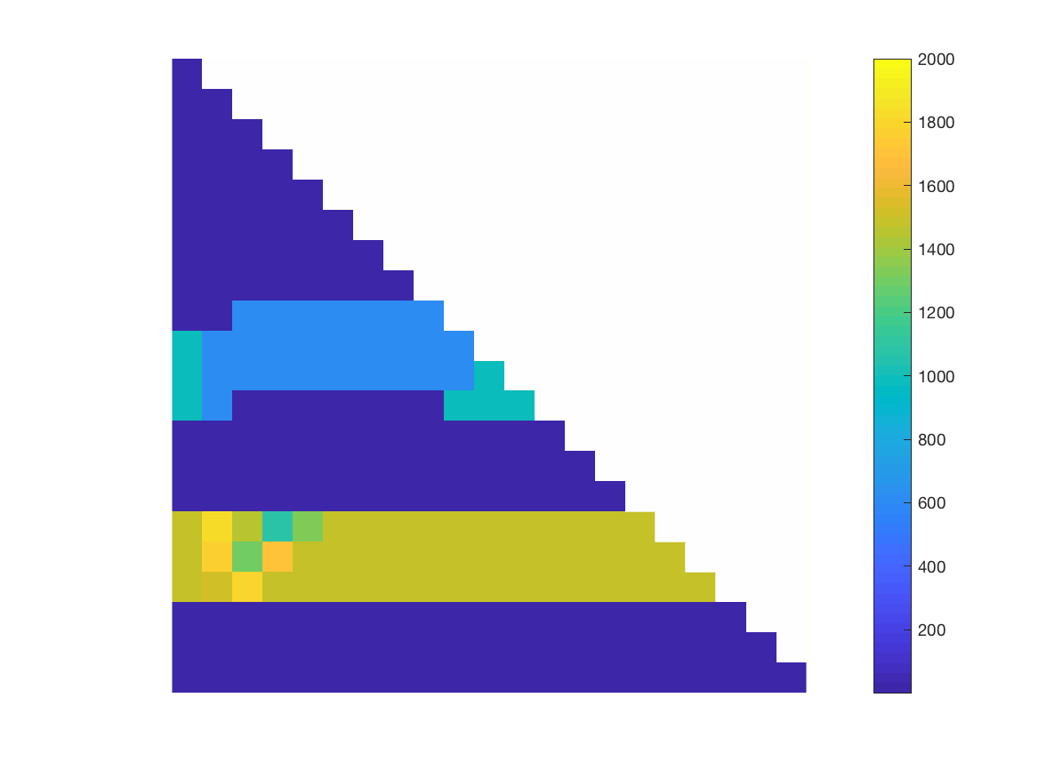
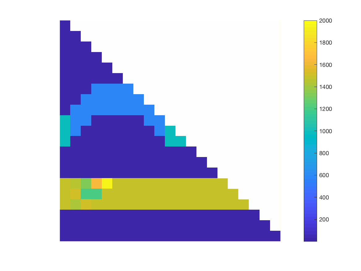
Figure 6: Samples of permeability fields in the target block $K_{0}$ in Experiment 2.

Next, for each realization, we compute the local multiscale basis functions and local coarse-scale stiffness matrix. In building the local snapshot space, we solve for harmonic extension of randomized fine-grid boundary conditions, so as to reduce the number of local problems to be solved. Local multiscale basis functions are then constructed by solving the spectral problem and multiplied the spectral basis functions with the multiscale partition of unity functions. With the offline space constructed, we compute the coarse-scale stiffness matrix. We use the training samples to build deep neural networks for approximating these GMsFEM quantities, and examine the performance of the approximations on the testing set.

Figures 7–9 show the comparison of the multiscale basis functions in 2 respective coarse neighborhoods. It can be observed that the predicted multiscale basis functions are in good agreement with the exact ones. In particular, the neural network successfully interprets the high conductivity regions as the support localization feature of the multiscale basis functions. Tables 5–6 record the mean error of the prediction by the neural networks, measured in the defined metric. Again, it can be seen that the prediction are of high accuracy. Table 7 records the mean error between the multiscale solution using the neural-network-based multiscale solver and using exact GMsFEM. we obtain a good approximation of the multiscale solution compared with the exact GMsFEM solver.

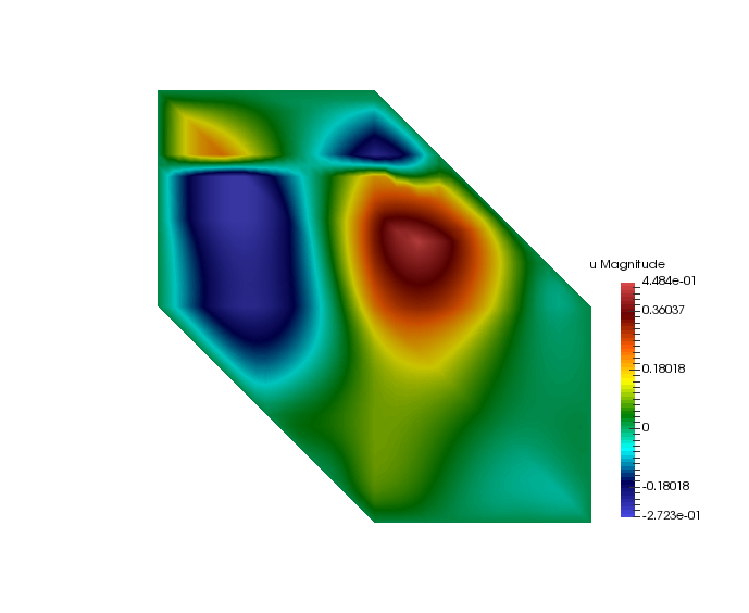
(a) Exact $\phi_{1}^{\omega_{1}}$

(b) Prediction $\phi_{1}^{\omega_{1},\text{pred}}$

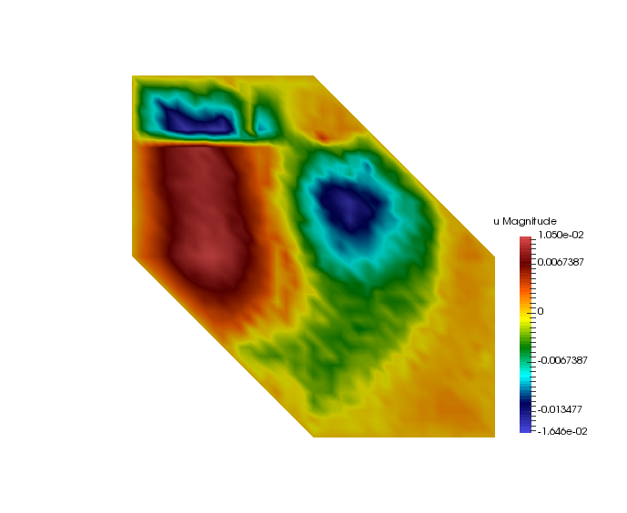
(c) Difference $\phi_{1}^{\omega_{1}}-\phi_{1}^{\omega_{1},\text{pred}}$

(d) Exact $\phi_{2}^{\omega_{1}}$

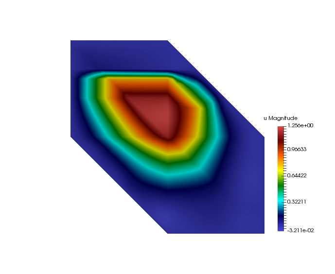
(e) Prediction $\phi_{2}^{\omega_{1},\text{pred}}$

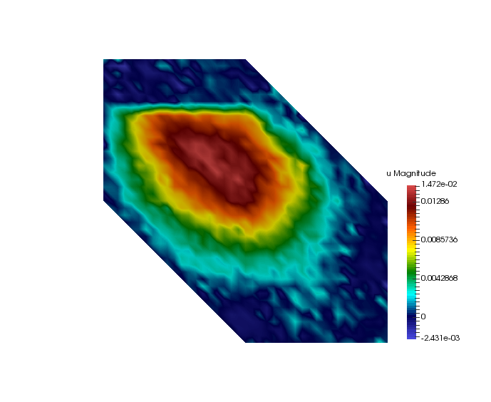
(f) Difference $\phi_{2}^{\omega_{1}}-\phi_{2}^{\omega_{1},\text{pred}}$

Figure 7: Exact multiscale basis functions $\phi_{m}^{\omega_{1}}$ and predicted multiscale basis functions $\phi_{m}^{\omega_{1},\text{pred}}$ in the coarse neighborhood $\omega_{1}$ in Experiment 2.

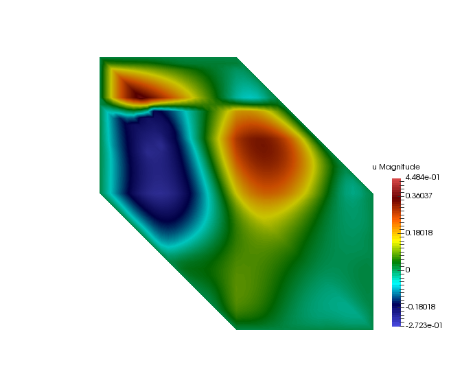
(a) Exact $\phi_{1}^{\omega_{2}}$

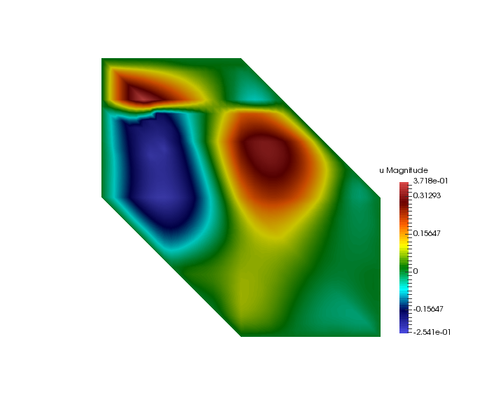
(b) Prediction $\phi_{1}^{\omega_{2},\text{pred}}$

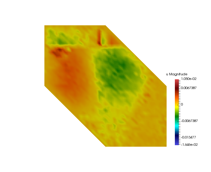
(c) Difference $\phi_{1}^{\omega_{2}}-\phi_{1}^{\omega_{2},\text{pred}}$

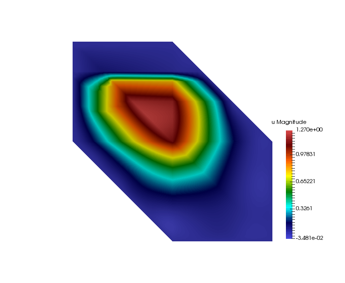
(d) Exact $\phi_{2}^{\omega_{2}}$

(e) Prediction $\phi_{2}^{\omega_{2},\text{pred}}$

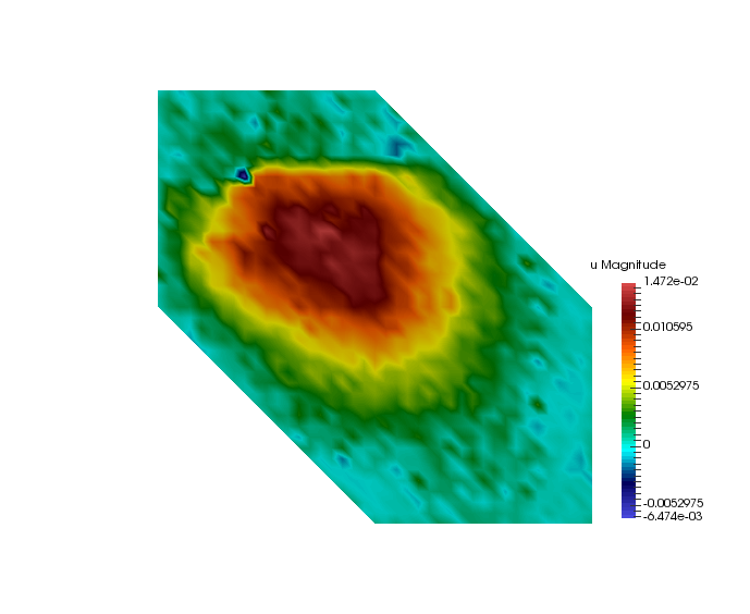
(f) Difference $\phi_{2}^{\omega_{2}}-\phi_{2}^{\omega_{2},\text{pred}}$

Figure 8: Exact multiscale basis functions $\phi_{m}^{\omega_{2}}$ and predicted multiscale basis functions $\phi_{m}^{\omega_{2},\text{pred}}$ in the coarse neighborhood $\omega_{2}$ in Experiment 2.

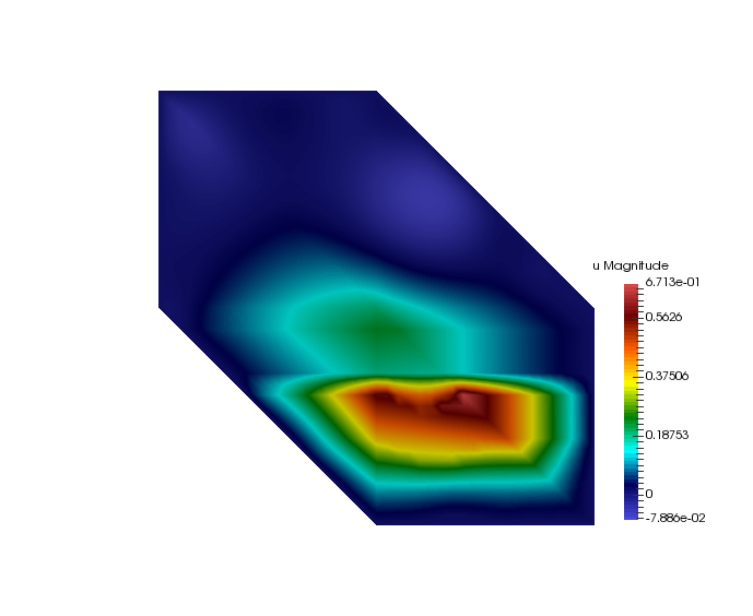
(a) Exact $\phi_{1}^{\omega_{3}}$

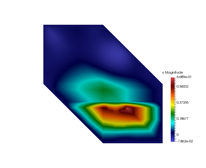
(b) Prediction $\phi_{1}^{\omega_{3},\text{pred}}$

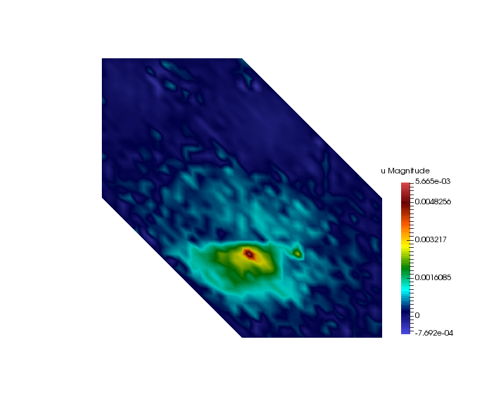
(c) Difference $\phi_{1}^{\omega_{3}}-\phi_{1}^{\omega_{3},\text{pred}}$

(d) Exact $\phi_{2}^{\omega_{3}}$

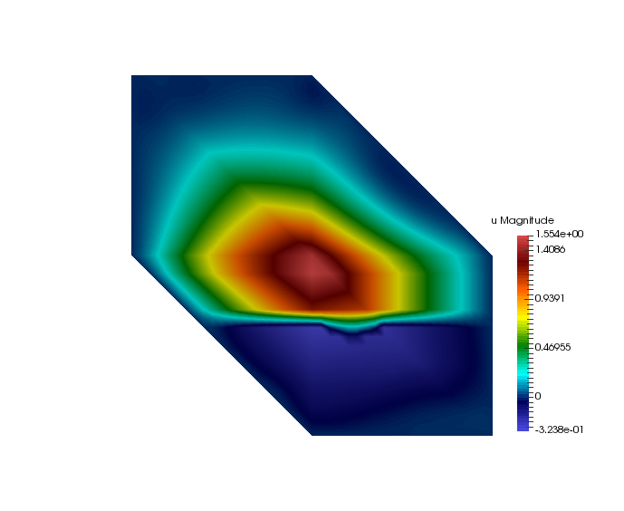
(e) Prediction $\phi_{2}^{\omega_{3},\text{pred}}$

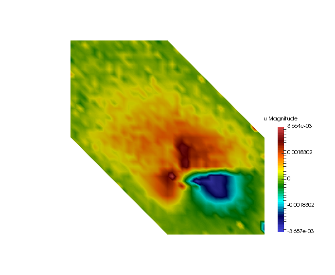
(f) Difference $\phi_{2}^{\omega_{3}}-\phi_{2}^{\omega_{3},\text{pred}}$

Figure 9: Exact multiscale basis functions $\phi_{m}^{\omega_{3}}$ and predicted multiscale basis functions $\phi_{m}^{\omega_{3},\text{pred}}$ in the coarse neighborhood $\omega_{3}$ in Experiment 2.

Basis	$\omega_{1}$		$\omega_{2}$		$\omega_{3}$
$m$	$e_{L^{2}}$	$e_{H^{1}}$	$e_{L^{2}}$	$e_{H^{1}}$	$e_{L^{2}}$	$e_{H^{1}}$
1	0.55	0.91	0.37	3.02	0.20	0.63
2	0.80	1.48	2.17	3.55	0.27	1.51

Table 5: Mean percentage error of multiscale basis functions $\phi_{m}^{\omega_{i}}$ in Experiment 2.

	$e_{\ell^{2}}$	$e_{\ell^{\infty}}$	$e_{F}$
Mean	0.75	0.72	0.80

Table 6: Percentage error of the local stiffness matrix $A_{c}^{K_{0}}$ in Experiment 2.

	$e_{L^{2}}$	$e_{a}$
Mean	0.03	0.26

Table 7: Percentage error of multiscale solution $u_{ms}$ in Experiment 2.

5 Conclusion

In this paper, we develop a method using deep learning techniques for fast computation of GMsFEM discretizations. Given a particular permeability field, the main ingredients of GMsFEM, including the multiscale basis functions and coarse-scale matrices, are computed in an offline stage by solving local problems. However, when one is interested in calculating GMsFEM discretizations for multiple choices of permeability fields, repeatedly formulating and solving such local problems could become computationally expensive or even infeasible. Multi-layer networks are used to represent the nonlinear mapping from the fine-scale permeability field coefficients to the multiscale basis functions and the coarse-scale parameters. The networks provide a direct fast approximation of the GMsFEM ingredients in a local neigorhood for any online permeability fields, in contrast to repeatedly formulating and solving local problems. Numerical results are presented to show the performance of our proposed method. We see that, given sufficient samples of GMsFEM discretizations for supervised training, deep neural networks are capable of providing reasonably close approximations of the exact GMsFEM discretization. Moreover, the small consistency error provides good approximations of multiscale solutions.

References

- [1] V. Calo, Y. Efendiev, J. Galvis, and G. Li. Randomized oversampling for generalized multiscale finite element methods. arXiv preprint, arXiv: 1409.7114, 2014.
- [2] Siu Wun Cheung, Eric T. Chung, Yalchin Efendiev, Eduardo Gildin, and Yating Wang. Deep global model reduction learning. arXiv preprint arXiv:1807.09335, 2018.
- [3] Siu Wun Cheung and Nilabja Guha. Dynamic data-driven bayesian GMsFEM. arXiv preprint arXiv:1806.05832, 2018.
- [4] François Chollet et al. Keras. https://keras.io, 2015.
- [5] E. Chung, Y. Efendiev, and C. Lee. Mixed generalized multiscale finite element methods and applications. SIAM Multicale Model. Simul., 13:338–366, 2014.
- [6] E. Chung, Y. Efendiev, and W. T. Leung. Generalized multiscale finite element method for wave propagation in heterogeneous media. SIAM Multicale Model. Simul., 12:1691–1721, 2014.
- [7] E. T. Chung, Y. Efendiev, and W. T. Leung. Residual-driven online generalized multiscale finite element methods. Journal of Computational Physics, 302:176–190, 2015.
- [8] Eric Chung, Yalchin Efendiev, and Thomas Y. Hou. Adaptive multiscale model reduction with generalized multiscale finite element methods. Journal of Computational Physics, 2016.
- [9] Eric T Chung, Efendiev, Wing Tat Leung, Maria Vasilyeva, and Yating Wang. Non-local multi-continua upscaling for flows in heterogeneous fractured media. arXiv preprint arXiv:1708.08379, 2018.
- [10] Balázs Csanád Csáji. Approximation with artificial neural networks. Faculty of Sciences, Etvs Lornd University, 24(48), 2001.
- [11] G. Cybenko. Approximations by superpositions of sigmoidal functions. Mathematics of Control, Signals, and Systems, 2(4):303–314, 1989.
- [12] Y. Efendiev, J. Galvis, and T. Y. Hou. Generalized multiscale finite element methods (gmsfem). Journal of Computational Physics, 251:116–135, 2013.
- [13] Y. Efendiev, J. Galvis, G. Li, and M. Presho. Generalized multiscale finite element methods. oversampling strategies. International Journal for Multiscale Computational Engineering, accepted, 12(6), 2013.
- [14] Y. Efendiev and T. Hou. Multiscale Finite Element Methods: Theory and Applications, volume 4 of Surveys and Tutorials in the Applied Mathematical Sciences. Springer, New York, 2009.
- [15] Yalchin Efendiev, Wing Tat Leung, Siu Wun Cheung, Nilabja Guha, Viet Ha Hoang, and Bani Mallick. Bayesian multiscale finite element methods. modeling missing subgrid information probabilistically. International Journal for Multiscale Computational Engineering, 2017.
- [16] Xavier Glorot, Antoine Bordes, and Yoshua Bengio. Deep sparse rectifier neural networks. In Proceedings of the Fourteenth International Conference on Artificial Intelligence and Statistics, pages 315–323. PMLR, 2011.
- [17] Boris Hanin. Universal function approximation by deep neural nets with bounded width and relu activations. arXiv:1708.02691, 2017.
- [18] Kaiming He, Xiangyu Zhang, Shaoqing Ren, and Jian Sun. Deep residual learning for image recognition. Proceedings of the IEEE conference on computer vision and pattern recognition, pages 770–778, 2016.
- [19] Geoffrey Hinton, Li Deng, Dong Yu, George E. Dahl, Abdel rahman Mohamed, Navdeep Jaitly, and Andrew Senior. Approximation capabilities of multilayer feedforward networks. IEEE Signal Processing Magazine, 29(6):82–97, 2012.
- [20] Kurt Hornik. Approximation capabilities of multilayer feedforward networks. Neural Networks, 4(2):251–257, 1991.
- [21] T. Hou and X.H. Wu. A multiscale finite element method for elliptic problems in composite materials and porous media. J. Comput. Phys., 134:169–189, 1997.
- [22] P. Jenny, S.H. Lee, and H. Tchelepi. Multi-scale finite volume method for elliptic problems in subsurface flow simulation. J. Comput. Phys., 187:47–67, 2003.
- [23] Yuehaw Khoo, Jianfeng Lu, and Lexing Ying. Solving parametric pde problems with artificial neural networks. arXiv:1707.03351, 2017.
- [24] Diederik P. Kingma and Jimmy Ba. Adam: A method for stochastic optimization. arXiv preprint arXiv:1412.6980, 2014.
- [25] Alex Krizhevsky, Ilya Sutskever, and Geoffrey E. Hinton. Imagenet classification with deep convolutional neural networks. Advances in neural information processing systems, pages 1097–1105, 2012.
- [26] Zhen Li and Zuoqiang Shi. Deep residual learning and pdes on manifold. arXiv:1708.05115., 2017.
- [27] H. Mhaskar Q. Liao and T. Poggio. Learning functions: when is deep better than shallow. arXiv:1603.00988v4, 2016.
- [28] M. Telgrasky. Benefits of depth in neural nets. JMLR: Workshop and Conference Proceedings, 49(123), 2016.
- [29] Yating Wang, Siu Wun Cheung, Eric T. Chung, Yalchin Efendiev, and Min Wang. Deep multiscale model learning. arXiv preprint arXiv:1806.04830, 2018.
- [30] E. Weinan and Bing Yu. The deep ritz method: A deep learning-based numerical algorithm for solving variational problems. Communications in Mathematics and Statistics, 6(1):1–12, 2018.
- [31] Yinhao Zhu and Nicholas Zabaras. Bayesian deep convolutional encoder–decoder networks for surrogate modeling and uncertainty quantification. Journal of Computational Physics, 366:415–447, 2018.