Fast, High-Quality Dual-Arm Rearrangement in Synchronous, Monotone Tabletop Setups

Abstract

Rearranging objects on a planar surface arises in a variety of robotic applications, such as product packaging. Using two arms can improve efficiency but introduces new computational challenges. This paper studies the structure of dual-arm rearrangement for synchronous, monotone tabletop setups and develops an optimal mixed integer model. It then describes an efficient and scalable algorithm, which first minimizes the cost of object transfers and then of moves between objects. This is motivated by the fact that, asymptotically, object transfers dominate the cost of solutions. Moreover, a lazy strategy minimizes the number of motion planning calls and results in significant speedups. Theoretical arguments support the benefits of using two arms and indicate that synchronous execution, in which the two arms perform together either transfers or moves, introduces only a small overhead. Experiments support these points and show that the scalable method can quickly compute solutions close to the optimal for the considered setup.

1 Introduction

Automation tasks in industrial and service robotics, such as product packing or sorting, often require sets of objects to be arranged in specific poses on a planar surface. Efficient and high-quality single-arm solutions have been proposed for such setups [19]. The proliferation of robot arms, however, including dual-arm setups, implies that industrial settings can utilize multiple robots in the same workspace (Fig 1). This work explores a) the benefits of coordinated dual-arm rearrangement versus single-arm, b) the combinatorial challenges involved and c) computationally efficient, high-quality and scalable methods.

A motivating point is that the coordinated use of multiple arms can result in significant improvements in efficiency. This arises from the following argument.

Lemma 1

There are classes of tabletop rearrangement problems, where a $k$-arm ($k\geq 2$) solution can be arbitrarily better than the optimal single-arm one.

For instance, assume two arms that have full (overhand) access to a unit square planar tabletop. There are $n$ objects on the table, divided into two groups of $\frac{n}{2}$ each. Objects in each group are $\varepsilon$-close to each other and to their goals. Let the distance between the two groups be on the order of $1$, i.e., the two groups are at opposite ends of the table. The initial position of each end-effector is $\varepsilon$-close to a group of objects. Let the cost of each pick and drop action be $c_{pd}$, while moving the end-effector costs $c_{t}$ per unit distance. Then, the $2$-arm cost is no more than $2nc_{pd}+2n\varepsilon c_{t}$. A single arm solution costs at least $2nc_{pd}+(2n-1)\varepsilon c_{t}+c_{t}$. If $c_{pd}$ and $\varepsilon$ are sufficiently small, the $2$-arm cost can be arbitrarily better than the single-arm one. The argument also extends to $k$-arms relative to $(k-1)$-arms.

In most practical setups, the expectation is that a $2$-arm solution will be close to half the cost (e.g., time-wise) of the single-arm case, which is a desirable improvement. While there is coordination overhead, the best $2$-arm solution cannot do worse; simply let one of the arms carry out the best single arm solution while the other remains outside the workspace. More generally:

Lemma 2

For any rearrangement problem, the best $k$-arm ($k\geq 2$) solution cannot be worse than an optimal single arm solution.

The above points motivate the development of scalable algorithmic tools for such dual-arm rearrangement instances. This work considers certain relaxations to achieve this objective. In particular, monotone tabletop instances are considered, where the start and goal object poses do not overlap. Furthermore, the focus is on synchronized execution of pick-and-place actions by the two arms. i.e., where the two arms simultaneously transfer (different) objects, or simultaneously move towards picking the next objects. Theoretical arguments and experimental evaluation indicate that the synchronization assumption does not significantly degrade solution quality.

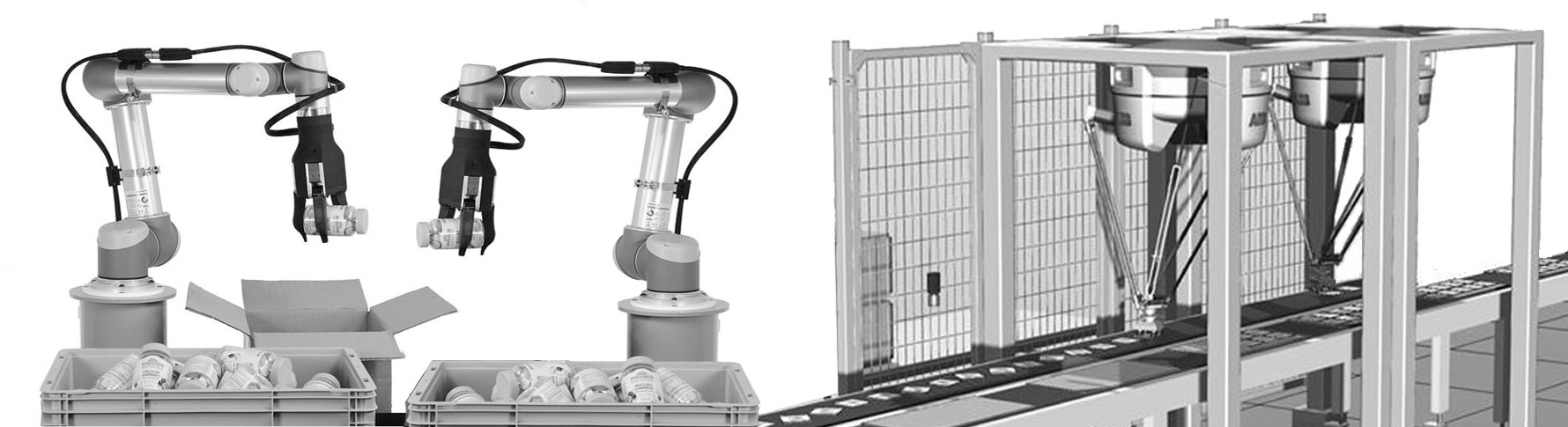
Figure 1: Example of dual-arm setups that can utilize algorithms proposed in this work.

The first contribution is the study of the combinatorial structure of synchronous, monotone dual-arm rearrangement. Then, a mixed integer linear programming (MILP) model is proposed that achieves optimal coordinated solutions in this domain. An efficient algorithm Tour_Over_Matching (TOM) is proposed that significantly improves in scalability. TOM first optimizes the cost of object transfers and assigns objects to the two arms by solving an optimal matching problem. It minimizes the cost of moves from an object’s goal to another object’s start pose per arm as a secondary objective by employing a TSP solution. Most of the computation time is spent on the many calls to a lower-level motion planner that coordinates the two arms. A lazy evaluation strategy is proposed, where candidate solution sequences are developed first and then motion plans are evaluated for them. The strategy results in significant computational improvement and minimizes the calls to the coordination motion planner. An analysis is also performed on the expected improvement in solution quality versus the single arm case, as well as the expected cost overhead from a synchronous solution.

Finally, experiments for i) a simple planar picker setting, and ii) a model of two 7-DOF Kuka arms, demonstrate a nearly two-fold improvement against the single arm case for the proposed approach in practice. The solutions are close to optimal for the dual-arm case and the algorithm exhibits good scalability. The computational costs of both the optimal and the proposed method are significantly improved from the lazy evaluation strategy.

2 Related Work

The current work dealing with dual-arm object rearrangement touches upon the challenging intersection of a variety of rich bodies of prior work. It is closely related to multi-robot planning and coordination. The challenge with multi-body planning is the high dimensionality of the configuration space. Optimal strategies were developed for simpler instances of the problem [35], although in general the problem is known to be computationally hard [33]. Decentralized approaches [40] also used velocity tuning [25] to deal with these difficult instances. General multi-robot planning tries to plan for multiple high-dimensional platforms [42, 15] using sampling-based techniques. Recent advances provide scalable [34] and asymptotically optimal [10] sampling based frameworks.

In some cases, by restricting the input of the problem to a certain type, it is possible to cast known hard instances of a problem as related algorithmic problems which have efficient solvers. For instance, unlabeled multi-robot motion planning can be reduced to pebble motion on graphs [1]; pebble motion can be reduced to network flow [46]; and single-arm object rearrangement can be cast as a traveling salesman problem [19]. These provide the inspiration to closely inspect the structure of the problem to derive efficient solutions.

In this work we leverage a connection between dual-arm rearrangement and two combinatorial problems: (1) optimal matching [11] and (2) TSP. On the surface the problem seems closely related to multi-agent TSP. A seminal paper [12] provides the formulation for k-TSP, with solutions that split a single tour. Prior work [28] has formulated the problem of multi-start to multi-goal k-TSP as an optimization task. Some work [13] deals with asymmetric edge weights which are more relevant to the problems of our interest.

The multi-arm rearrangement can also be posed as an instance of multi vehicle pickup and delivery (PDP) [27]. Prior work [8] has applied the PDP problem to robots, taking into account time windows and robot-robot transfers. Some seminal work [24, 30] has also explored its complexity, and concedes to the hardness of the problem, while others have studied cost bounds [38]. ILP formulations [30] have also been proposed. Typically this line of work ignores coordination costs, though some methods [5] reason about it once candidate solutions are obtained.

Navigation among movable objects deals with the combinatorial challenges of multiple objects [43, 39] and has been shown to be a hard problem, and extended to manipulation applications [37]. Despite a lot of interesting work on challenges of manipulation and grasp planning, the current work shall make assumptions that avoid complexities arising from them. Manipulators opened the applications of rearrangement planning [3, 26], including instances where objects can be grasped only once or monotone [37], as well as non-monotone instances [20, 36]. Efficient solutions to assembly planning problems [44, 18] typically assumes monotonicity, as without it the problem becomes much more difficult. Recent work has dealt with the hard instances of task planning [4, 7] and rearrangement planning [22, 23, 19]. Sampling-based task planning has made a recent push towards guarantees of optimality [41, 31]. These are broader approaches that are invariant to the combinatorial structure of the application domain. The current work draws inspiration from these varied lines of research.

General task planning methods are unaware of the underlying structure studied in this work. Single-arm rearrangement solutions will also not effective in this setting. The current work tries to bridge this gap and provide insights regarding the structure of dual-arm rearrangement. Under assumptions that enable this study, an efficient solution emerges for this problem.

3 Problem Setup and Notation

Consider a planar surface and a set of $n$ rigid objects $\mathcal{O}=\{o_{1},o_{2}\cdots o_{n}\}$ that can rest on the surface in stable poses $p_{i}\in\mathcal{P}_{i}\subset SE(3)$. The arrangement space $\mathcal{A}=\mathcal{P}_{1}\times\mathcal{P}_{2}\ldots\times\mathcal{P}_{n}$ is the Cartesian product of all $\mathcal{P}_{i}$, where $A=(p_{1},\ldots,p_{n})\in\mathcal{A}$. In valid arrangements $\mathcal{A}_{\rm val}\subset\mathcal{A}$, the objects are pairwise disjoint.

Figure 2: An example of object rearrangement involving two robotic arms. Initial (left) and final (right) object configuration.

Two robot arms $m^{1}$ and $m^{2}$ can pick and place the objects from and to the surface. $\mathbb{C}_{{\rm free}}^{k}$ is the set of collision-free configurations for arm $m^{k}$ (while ignoring possible collisions with objects or the other arm), and is assumed here to be a subset of $\mathbb{R}^{d}$. A path for $m^{k}$ is denoted as $\pi^{k}:[0,1]\rightarrow\mathbb{C}_{{\rm free}}^{k}$ and includes picking and placing actions. Let $\mathbb{C}_{{\rm free}}^{i}(\pi^{j})$ represent the collision free $\mathbb{C}$-space for $m^{i}$, given that $m^{j}$ moves along $\pi^{j}$. This is a function of the paths’ parametrization. The space of dual-arm paths $\mathcal{D}$ denotes pairs of paths for the two arms: $D=(\pi^{1},\pi^{2})\in\mathcal{D}$. Then, $A(A_{\rm init},D)$ is the resulting arrangement when the objects are at $A_{\rm init}$ and moved according to $D$. Let $\textup{cost}(D):\mathcal{D}\rightarrow\mathbb{R}$ be a cost function over dual-arm paths.

Definition 1 (Optimal Dual-arm Rearrangement)

Given arms $m^{1}$, $m^{2}$ and objects $\mathcal{O}$ to be moved from initial arrangement $A_{\rm init}\in\mathcal{A}_{\rm val}$ to target arrangement $A_{\rm goal}\in\mathcal{A}_{\rm val}$, the optimal dual-arm rearrangement problem asks for a dual-arm path $D^{*}\in\mathcal{D}$, which satisfies the following constraint:

$$D^{*}=(\pi^{*1},\pi^{*2})\ |\ A(A_{\rm init},D^{*})=A_{\rm goal}\textrm{ and }\pi^{*i}\in\mathbb{C}_{{\rm free}}^{i}(\pi^{*j})\vspace{-.05in}$$ (1)

and optimizes a cost function: $D^{*}=\underset{\forall D\in\mathcal{D}}{\mathtt{argmin}}\ \textup{cost}(D).$

A set of assumptions are introduced to deal with the problem’s combinatorics. The reachable task-space $\mathcal{T}^{k}\subset SE(3)$ of arm $m^{k}$ is the set of $SE(3)$ poses that objects attached to the arm’s end effector can acquire.

Let the ordered set of objects moved during the arm path $\pi^{i}$ be denoted as $\bar{\mathcal{O}}(\pi^{k})$. In general, an object can appear many times in $\bar{\mathcal{O}}(\pi^{k})$. The current work, however, focuses on monotone instances, where each object is moved once.

Assumption 1 (Monotonicity)

There are dual-arm paths $D=(\pi^{1},\pi^{2})$ that satisfy Eq. 1, where each object $o_{i}\in\mathcal{O}$ appears once in $\bar{\mathcal{O}}(\pi^{1})$ or $\bar{\mathcal{O}}(\pi^{2})$.

For the problem to be solvable, all objects are reachable by at least one arm at both $A_{\rm init}$ and $A_{\rm goal}$: $\forall\ p_{i}\in A_{\rm init}\textrm{ and }\forall\ p_{j}\in A_{\rm goal}\textrm{ and }\exists\ k\in[1,2]:p_{i},p_{j}\subset\mathcal{T}^{k}$. The focus will be on simultaneous execution of transfer and move paths.

Transfers: Dual-arm paths $T(\pi^{1}_{i},\pi^{2}_{i})\in\mathcal{D}$, where $\bar{\mathcal{O}}(\pi^{k}_{i})=o^{k}_{i}$ and each $m^{k}$:

• starts the path in contact with an object $o^{k}_{i}$ at its initial pose in $A_{\rm init}$,

• and completes it in contact with object $o^{k}_{i}$ at its final pose in $A_{\rm goal}$.

Moves or Transits: Paths $M(\pi^{1}_{i\rightarrow i^{\prime}},\pi^{2}_{i\rightarrow i^{\prime}})\in\mathcal{D}$, $\bar{\mathcal{O}}(\pi^{1}_{i\rightarrow i^{\prime}})=\emptyset$, and each $m^{k}$:

• starts in contact with object $o^{k}_{i}$ at its final pose in $A_{\rm goal}$,

• and completes it in contact with object $o^{k}_{i^{\prime}}$ at its initial pose in $A_{\rm init}$.

Assumption 2 (Synchronicity)

Consider dual-arm paths, which can be decomposed into a sequence of simultaneous transfers and moves for both arms:

$$D=\left(T(\pi^{1}_{1},\pi^{2}_{1}),M(\pi^{1}_{1\rightarrow 2},\pi^{2}_{1\rightarrow 2}),\ldots,M(\pi^{1}_{\ell-1\rightarrow\ell},\pi^{2}_{\ell-1\rightarrow\ell}),T(\pi^{1}_{\ell},\pi^{2}_{\ell})\right).\vspace{-.05in}$$ (2)

For simplicity, Eq. 2 does not include an initial move from $q^{k}_{\rm safe}\in\mathbb{C}_{{\rm free}}^{k}$ and a final move back to $q^{k}_{\rm safe}$. An odd number of objects can also be easily handled. Then, the sequence of object pairs moved during a dual-arm path as in Eq. 2 is:

$${{\Omega}}(D)=\left({\omega}_{i}=(o_{i}^{1},o_{i}^{2})\ |\ i,j\in[1\cdots\ell],\bigcup_{i}(o_{i}^{1}\cup o_{i}^{2})=\mathcal{O},\forall k,k^{\prime}\in[1,2],o_{i}^{k}\neq o_{j}^{k^{\prime}}\right).\vspace{-.1in}$$

Given the pairs of objects ${\omega}_{i}$, it is possible to express a transfer as $T({\omega}_{i})$ and a move as $M({\omega}_{i\rightarrow j})$. Then, $D({{\Omega}})$ is the synchronous, monotone dual-arm path due to ${{\Omega}}=({\omega}_{1},\ldots,{\omega}_{\ell})$, i.e., $D({{\Omega}})=(T({\omega}_{1}),M({\omega}_{1\rightarrow 2}),\ldots,M({\omega}_{\ell-1\rightarrow\ell}),T({\omega}_{\ell})).$

Assumption 3 (Object Non-Interactivity)

There are collision-free transfers $T({\omega}_{i})$ and moves $M({\omega}_{i\rightarrow i^{\prime}})$ regardless of the object poses in $A_{\rm init}$ and $A_{\rm goal}$.

This entails that there is no interaction between the $n$ resting objects and the arms during transits. Similarly, there are no interactions between the arm-object system and the $n-2$ resting objects during the transfers. Collisions involving the arms, static obstacles and picked objects are always considered.

The metric this work focuses on relates to makespan and minimizes the sum of the longest distances traveled by the arms in each synchronized operation. Let $\|\pi^{k}\|$ denote the Euclidean arc length in $\mathbb{C}_{{\rm free}}^{k}\subset\mathbb{R}^{d}$ of path $\pi^{k}$. Then, for transfers $\textup{cost}(T(\pi^{1}_{i},\pi^{2}_{i}))=\max\{\|\pi^{1}_{i}\|,\|\pi^{2}_{i}\|\}$. Similarly, $\textup{cost}(M(\pi^{1}_{i\rightarrow i^{\prime}},\pi^{2}_{i\rightarrow i^{\prime}}))=\max\{\|\pi^{1}_{i\rightarrow i^{\prime}}\|,\|\pi^{2}_{i\rightarrow i^{\prime}}\|\}$. Then, over the entire dual-arm path $D$ define:

$$\textup{cost}(D)=\sum_{i=1}^{\ell}\textup{cost}(T({\omega}_{i}))+\sum_{i=1}^{\ell-1}\textup{cost}(M({\omega}_{i\rightarrow i+1})).\vspace{-.1in}$$ (3)

Note that the transfer costs do not depend on the order with which the objects are moved but only on the assignment of objects to arms. The transit costs arise out of the specific ordering in ${{\Omega}}(D)$. Then, for the setup of Definition 1 and under Assumptions 1-3, the problem is to compute the optimal sequence of object pairs ${{\Omega}}^{*}$ so that $D({{\Omega}}^{*})$ satisfies Eq. 1 and minimizes the cost of Eq. 3.

Note on Assumptions: This work restricts the study to a class of monotone problems that relate to a range of industrial packing and stowing applications. The monotonicity assumption is often used in manageable variants of well-studied problems [44, 18]. A monotone solution also implies that every object’s start and target is reachable by at least one arm. To deal with cases where the number of reachable objects is unbalanced between the two arms, a NO_ACT task assignment is introduced and considered in Section 6.

The synchronicity assumption allows to study the combinatorial challenges of the problem, which do not relate to the choice of time synchronization of different picks and placements. Section 6 describes the use of ${\tt dRRT^{*}}$[10] as the underlying motion planner that can discover solutions that can synchronize arm motions for simultaneous picks, and simultaneous placements. The synchronicity assumption is relaxed through smoothing (Section 6).

The non-interactivity assumption comes up naturally in planar tabletop scenarios with top-down picks or delta robots. Such scenarios are popular in industrial settings. Once the object is raised from the resting surface, transporting it to its target does not introduce interactions with the other resting objects. This assumption is also relaxed in Section 6, with a lazy variant of the proposed method. Once a complete candidate solution is obtained, collision checking can be done with everything in the scene.

Overall, under the assumptions, the current work identifies a problem structure, which allows arguments pertaining to the search space, completeness, and optimality. Nevertheless, the smoothed, lazy variant of the proposed method will still return effective solutions in practice, even if these assumptions do not hold.

4 Baseline Approaches and Size of Search Space

This section highlights two optimal strategies to discover $D({{\Omega}}^{*})$: a) exhaustive search, which reveals the search space of all possible sequences of object pairs ${{\Omega}}$ and b) an MILP model. Both alternatives, however, suffer from scalability issues as for each possible assignment, it is necessary to solve a coordinated motion planning problem for the arms. This motivates minimizing the number of assignments ${\omega}$ considered, and the number of motion planning queries it requires for discovering $D({{\Omega}}^{*})$, while still aiming for high quality solutions.

Exhaustive Search: The exhaustive search approach shown in Fig. 3 is a brute force expansion of all possible sequences of object pairs ${{\Omega}}$. Nodes correspond to transfers $T({\omega}_{i})$ and edges are moves $M({\omega}_{i\rightarrow i{{}^{\prime}}})$. The approach evaluates the cost for all possible branches to return the best sequence ${{\Omega}}$. The total number of nodes is in the order of $O(n!)$, expressed over the levels $L$ of the search tree as:

$${\prescript{n\mkern-2.5mu}{}{P}_{2}}+{\prescript{n\mkern-2.5mu}{}{P}_{2}}\times{\prescript{n-2\mkern-2.5mu}{}{P}_{2}}+...+{\prescript{n\mkern-2.5mu}{}{P}_{2}}\times{\prescript{n-2\mkern-2.5mu}{}{P}_{2}}\times{\prescript{n-4\mkern-2.5mu}{}{P}_{2}}...\times{\prescript{2\mkern-2.5mu}{}{P}_{2}}=\sum_{L=1}^{n/2}{\ \prod_{k=0}^{2L-1}{(n-k)}},\vspace{-0.15in}$$

where $\prescript{n\mkern-2.5mu}{}{P}_{k}$ denotes the number of $k$-permutations of $n$.

Figure 3: Search tree for 4 objects. In node $XY$, $m^{1}$ transfers object $X$, and $m^{2}$ transfers $Y$. An edge is a transit to the next node.

Motion plans can be reused, however, and repeated occurrences of $T({\omega}_{i})$ and $M({\omega}_{i\rightarrow i^{\prime}})$ should be counted only once for a total of:

• ${\prescript{n\mkern-2.5mu}{}{P}_{2}}$ transfers of objects, and

• ${{\prescript{n\mkern-2.5mu}{}{P}_{2}}\times\prescript{n-2\mkern-2.5mu}{}{P}_{2}}$ transits between all possible valid ordered pairs of ${\omega}$.

Additional motion plans are needed for the initial move from $q_{\rm safe}^{k}$ and the return to it at the end of the process, introducing $2\times\prescript{n\mkern-2.5mu}{}{P}_{2}$ transits:

$$\textrm{\# of Transfers}+\textrm{\# of Moves}={\prescript{n\mkern-2.5mu}{}{P}_{2}}+\Big{(}({{\prescript{n\mkern-2.5mu}{}{P}_{2}}\times\prescript{n-2\mkern-2.5mu}{}{P}_{2}})+(2\times{\prescript{n\mkern-2.5mu}{}{P}_{2}})\Big{)}\vspace{-0.2in}$$ (4)

This returns optimal synchronized solution but performs an exhaustive search and requires exponentially many calls to a motion planner.

MILP Formulation: Mixed Integer Linear Programming (MILP) formulations can utilize highly optimized solvers [17]. Prior work has applied these techniques for solving m-TSP [28, 13] and pickup-and-delivery problems [8, 30], but viewed these problems in a decoupled manner. This work outlines an MILP formulation for the synchronized dual-arm rearrangement problem that reasons about coordination costs arising from arm interactions in a shared workspace.

Graph Representation: The problem can be represented as a directed graph where each vertex $v={\omega}_{v}=(o_{v}^{1},o_{v}^{2})$ corresponds to a transfer $T({\omega}_{u})$ and edges $e(u,v)$ are valid moves $M({\omega}_{u\rightarrow v})$. A valid edge $e(u,v)$ is one where an object does not appear more than once in the transfers of nodes $u$ and $v$. The cost of a directed edge $e(u,v)$ encodes both the cost of the transfer $T({\omega}_{v})$ and the cost of the move $M({\omega}_{u\rightarrow v})$. There is also a vertex $S$, which connects moves from and to the safe arm configurations $q^{k}_{\rm safe}$. The directed graph $\hat{G}(\hat{V},\hat{E})$ is defined:

$$\hskip 36.135pt\hat{V}=\{v={\omega}_{v}=(o_{v}^{1},o_{v}^{2})\ |\ \forall\ o_{v}^{1},o_{v}^{2}\in\mathcal{O},o_{v}^{1}\neq o_{v}^{2}\}\cup\{S\}$$

$$\hat{E}=\{e(u,v)\ |\ \forall\ u,v\in\hat{V}\textrm{ so that }u\neq v,\ o_{v}^{k}\neq o_{u}^{\ell}\ \forall\ k,\ell\in[1,2]\}$$

$$\cup\ \{e(S,v)\ \forall\ v\in\hat{V}\setminus S\}\cup\{e(v,S)\ \forall\ v\in\hat{V}\setminus S\}$$

$$cost_{e(u,v)}=\textup{cost}(u)+\textup{cost}(u,v)=\textup{cost}(T({\omega}_{u}))+\textup{cost}(M({\omega}_{u\rightarrow v}))$$

Let $\textup{cost}(S)=0$. The total number of motion planning queries needed to be answered to define the edge costs is expressed in Eq. 4. The formulation proposed in this section tries to ensure the discovery of ${{\Omega}}^{*}$ on $\hat{G}$ as a tour that starts and ends at $S$, while traversing each vertex corresponding to ${{\Omega}}^{*}$. To provide the MILP formulation, define $\delta_{\rm in}(v)$ as the in-edge set $v$, and $\delta_{\rm out}(v)$ as the out-edge set. Then, $\gamma(o)$ is the object coverage set $\gamma(o)=\{e(u,v)\ |\ e\in\hat{E},o\in{\omega}_{u}\}$, i.e., all the edges that transfer $o$.

Model: Set the optimization objective as: $\ \ \min\sum_{e\in\hat{E}}cost_{e}x_{e}\$                   [A]
Eq. [B] below defines indicator variables. Eqs. [C-E] ensure edge-flow conserved tours. Eqs. [F-G] force $S$ to be part of the tour. Eq. [H] transfers every object only once. Eq. [I] lazily enforces the tour to be of length $\frac{n}{2}+1$. While the number of motion-planning queries to be solved is the same as in exhaustive search, efficient MILP solvers [17] provide a more scalable search process.

$$x_{e}\in\{0,1\} \ \ \forall e\in\hat{E}$$ [B]

$$\sum_{e\in\delta_{\rm in}(v)}x_{e}\leq 1 \ \ \forall v\in\hat{V}$$ [C]

$$\sum_{e\in\delta_{\rm out}(v)}x_{e}\leq 1 \ \ \forall v\in\hat{V}$$ [D]

$$\sum_{e\in\delta_{\rm in}(v)}x_{e}=\sum_{e\in\delta_{\rm out}(v)}x_{e} \ \ \forall v\in\hat{V}$$ [E]

$$\sum_{e\in\delta_{\rm in}(S)}x_{e}=1$$ [F]

$$\sum_{e\in\delta_{\rm out}(S)}x_{e}=1$$ [G]

$$\sum_{e\in\gamma(o)}x_{e}=1 \ \ \forall o\in\mathcal{O}$$ [H]

$$\sum_{e(u,v)\in\mathfrak{T}}x_{e}<|\mathfrak{T}| \ \ \forall\mathfrak{T}\subset\hat{V},|\mathfrak{T}|\leq\frac{n}{2}$$ [I]

5 Efficient Solution via Tour over Matching

The optimal baseline methods described above highlight the problem’s complexity. Both methods suffer from the large number of motion-planning queries they have to perform to compute the cost measures on the corresponding search structures. For this purpose it needs to be seen whether it is possible to decompose the problem into solvable sub-problems.

Importance of Transfers: In order to draw some insight, consider again the tabletop setup with a general cost measure of $c_{t}$ per unit distance. Lemma 1 suggests that under certain conditions, there may not be a meaningful bound on the performance ratio between a $k$-arm solution and a single-arm solution. This motivates the examination of another often used setting—randomly chosen non-overlapping start and goal locations for $n$ objects (within a unit square). In order to derive a meaningful bound on the benefit of using a $2$-arm solution to a single-arm solution, we first derive a conservative cost of a single-arm solution. A single-arm optimal cost has three main parts: 1) the portion of the transfer cost involving the pickup and drop-off of the $n$ objects with a cost of $C_{pd}=nc_{pd}$, 2) the remaining transfer cost from start to goal for all objects $C_{sg}$, and 3) the transit cost going from the goals to starts $C_{gs}$. The single arm cost is

$$C_{\rm single}=nc_{pd}+C_{sg}+C_{gs}.\vspace{-0.1in}$$ (5)

To estimate Eq. 5, first note that the randomized setup will allow us to obtain the expected $C_{sg}$[29] as $\frac{2+\sqrt{2}+5\ln(1+\sqrt{2})}{15}nc_{t}\approx 0.52nc_{t}$. Approximate $C_{gs}$ by simply computing an optimal assignment of the goals to the starts of the objects excluding the matching of the same start and goal. Denoting the distance cost of this matching as $C_{gs}^{M}$, clearly $C_{gs}>C_{gs}^{M}$ because the paths produced by the matching may form multiple closed loops instead of the desired single loop that connects all starts and goals. However, the number of loops produced by the matching procedure is on the order of $\ln n$ and therefore, $C_{gs}<C_{gs}^{M}+c_{t}\ln n$, by [38]. By [2], $C_{gs}^{M}=\Theta(\sqrt{n\ln n})$. Putting these together, we have,

$\Theta(c_{t}\sqrt{n\ln n})=C_{gs}^{M}<C_{gs}<C_{gs}^{M}+c_{t}\ln n=\Theta(c_{t}\sqrt{n\ln n})+c_{t}\ln n$

which implies that $C_{gs}\approx C_{gs}^{M}$ because for large $n$, $\ln n\ll\sqrt{n\ln n}$. It is estimated in [45] that $C_{gs}^{M}\approx 0.44\sqrt{n\ln n}c_{t}$ for large $n$. Therefore,

$$C_{\rm single}\approx nc_{pd}+(0.52n+0.44\sqrt{n\ln n})c_{t}\approx(c_{pd}+0.52c_{t})n$$ (6)

noting that the $0.44\sqrt{n\ln n}c_{t}$ term may also be ignored for large $n$. The cost of dual arm solutions will be analyzed in Section 7.

Lemma 3

For large $n$, the transfers dominate the cost of the solution.

We formulate a strategy to reflect this importance of transfers. The proposed approach gives up on the optimality of the complete problem, instead focusing on a high-quality solution, which:

• first optimizes transfers and selects an assignment of object pairs to arms,

• and then considers move costs and optimizes the schedule of assignments.

This ends up scaling better by effectively reducing the size of the search space and performing fewer motion planning queries. It does so by optimizing a related cost objective and taking advantage of efficient polynomial-time algorithms.

$$\begin{split}\mathcal{G}(\mathcal{V},\mathcal{E})\\ \mathcal{V}=\{{v}=o,\forall o\in\mathcal{O}\}\\ \mathcal{E}=\{{e}(u,v):{\omega}=(u,v),\forall u,v\in\mathcal{V}\}\\ \textup{cost}({e}(u,v))=\textup{cost}(T({\omega}=(u,v)))\end{split}$$ (7)

$$\begin{split}\mathcal{G}_{{\Gamma}}(\mathcal{V}_{{\Gamma}},\mathcal{E}_{{\Gamma}})\\ \mathcal{V}_{{\Gamma}}=\{{v}={\omega},\forall{\omega}\in\{{{\Omega}}\}^{*}\}\cup\{{\omega}_{S}\}\\ \mathcal{E}_{{\Gamma}}=\{{e}(u,v):{\omega}_{u\rightarrow v},\forall u,v\in\mathcal{V}_{{\Gamma}}\}\\ \textup{cost}({e}(u,v))=\textup{cost}(M({\omega}_{u\rightarrow v}))\end{split}$$ (8)

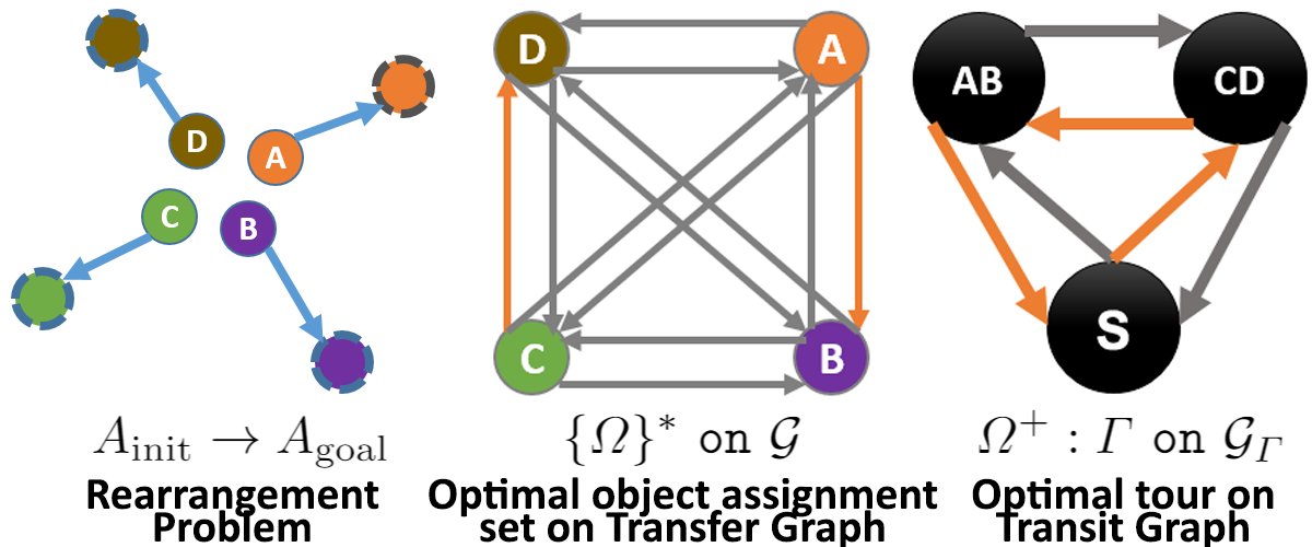
Figure 4: (left) A dual-arm rearrangement problem. (middle) The same problem as minimum weight edge matching on a fully connected directed graph of transfers. (right) The ordering of the object-arm assignments from an optimal tour over a transit graph.

Foundations: Consider a complete weighted directed graph $\mathcal{G}(\mathcal{V},\mathcal{E})$ (Eq. 7), where ${v}\in\mathcal{V}$ corresponds to a single object $o$. Each directed edge, ${e}=(o_{i},o_{j})\in\mathcal{E}$ is an ordered pair of objects $o_{i}$ and $o_{j}$, where the order determines the assignment of an object to an arm $m^{1}$ or $m^{2}$. The cost of an edge $\textup{cost}({e})$ is the coordinated motion planning cost of performing the transfer corresponding to ${\omega}=(o_{i},o_{j})$. For instance, as shown in Fig 4(middle), ${e}(A,B)$ corresponds to $m^{1}$ transferring ‘A’, while $m^{2}$ transfers ‘B’, and the $\textup{cost}({e}(A,B))=\textup{cost}(T({\omega}=(A,B))$ is the cost of such a concurrent motion. Note that these costs refer to only the transfer costs i.e., starting from the arms picking up the objects $A$ and $B$ at the initial poses(as shown in Fig 4(left)), and moving them to their target poses. It should also be noted that since the arms are different, in general, $\textup{cost}({e}(A,B))$ is not necessarily equal to $\textup{cost}({e}(B,A))$.

Following the observation made in Eq. 3, the cost of the transfers can be reasoned about independent of their order. Define $\{{{\Omega}}\}$ as the unordered set of ${\omega}\in{{\Omega}}$, then unordered transfer cost component corresponds to $\sum_{{\omega}\in\{{{\Omega}}\}}\textup{cost}(T({\omega}))$. Since $\mathcal{G}$ is a complete graph where every edge corresponds to every possible valid ${\omega}$, $\{{{\Omega}}\}$ must also be a part of $\mathcal{G}$. From the construction of the graph $\mathcal{G}$, $\{{{\Omega}}\}\subset\mathcal{E}$. By definition, a candidate solution of a monotone dual-arm rearrangement problem must transfer every object exactly once. In terms of the graph, this means that in the subset of edges $\{{{\Omega}}\}$ every vertex appears in only one edge. We arrive at the following crucial observation.

Lemma 4 (Perfect Matching)

Every candidate solution to a monotone dual-arm rearrangement problem comprises of a set of unordered object-to-arm assignments $\{{{\Omega}}\}$ that is also a perfect matching solution on $\mathcal{G}$.

As per the decomposition of the costs in Eq. 3, it follows that the $\textup{cost}(\{{{\Omega}}\})$ corresponds to the cost of the transfers in the solution. Given the reduction to edge-matching, the solution to the minimum-weight perfect edge matching problem on such a graph would correspond to a $\{{{\Omega}}\}$ that optimizes the cost of transfers of all the objects.

Lemma 5 (Optimal Matching)

The set of object-to-arm assignments $\{{{\Omega}}\}^{*}$ that minimizes the cost of object transfers is a solution to the minimum-weight perfect matching problem on $\mathcal{G}$.

Once such an optimal assignment $\{{{\Omega}}\}^{*}$ is obtained, the missing part of the complete solution is the set of transits between the object transfers and their ordering. Construct another directed graph $\mathcal{G}_{{\Gamma}}$ (Eqs. 8), where the vertices comprise of the ${\omega}\in\{{{\Omega}}\}^{*}$. An edge $e({\omega}_{u\rightarrow v})$ between any two vertices corresponds to the coordinated transit motion between them. For instance, as in Fig 4(right) for an edge between ${\omega}(A,B)$ and ${\omega}(C,D)$, $m^{1}$ moves from the target pose of object ‘A’ to the starting pose of object ‘C’, and similarly $m^{2}$ moves from the target of ‘B’ to the start of ‘D’. An additional vertex corresponding to the starting(and ending) configuration of the two arms ($S$) is added to the graph. The graph is fully connected again to represent all possible transits or moves.

A complete candidate solution to the problem now requires the sequence of ${\omega}$. By definition of the edges, the complete solution begins at $S$ and also ends there. This is a complete tour over $\mathcal{G}_{{\Gamma}}$, that visits all the vertices i.e., an ordered sequence of vertices ${\Gamma}=({S},{{\Omega}}_{\Gamma},{S})$.

Lemma 6 (Tour)

Any complete tour ${\Gamma}$ over the graph $\mathcal{G}_{{\Gamma}}$, corresponds to a sequence of object-to-arm assignments ${{\Omega}}_{\Gamma}$ and is a candidate solution to the synchronous dual-arm rearrangement problem.

Let $\mathbb{P}^{\{{{\Omega}}\}}$ represent the set of all possible ordering of the elements in $\{{{\Omega}}\}$. This means, any candidate tour corresponds to a ${{\Omega}}_{\Gamma}\in\mathbb{P}^{\{{{\Omega}}\}}$. An optimal tour on $\mathcal{G}_{{\Gamma}}$ minimizes the transit costs over the all possible candidate solutions in $\mathbb{P}^{\{{{\Omega}}\}^{*}}$.

$${{\Omega}}^{+}=\underset{{{\Omega}}\in\mathbb{P}^{\{{{\Omega}}\}^{*}}}{\mathtt{argmin}}\ \sum_{e(u,v)\in{\Gamma}}\textup{cost}({M}({\omega}_{u\rightarrow v})))\vspace{-0.05in}$$ (9)

This differs from the true optimal ${{\Omega}}^{*}$, since the second step of finding the optimal transit tour only operates over all possible solutions that include the optimally matched transfers obtained in the first step. The insight here is that, even though ${{\Omega}}^{+}$ reports a solution to a hierarchical optimization objective, the algorithm operates over a much smaller search space, and operates over sub-problems which are more efficient to solve than the baselines.

Algorithm: This section describes the algorithm Tour_Over_Matching (TOM) outlined in the previous section. The steps correspond to Algo 1.

$\mathtt{transfer\_graph}$: This function constructs a directed graph $\mathcal{G}$ defined by Eqs. 7. This step creates a graph with $n$ vertices and $\prescript{n\mkern-2.5mu}{}{P}_{2}$ edges.

1 $\mathcal{G}\leftarrow\mathtt{transfer\_graph}(\mathcal{O},A_{\rm init},A_{\rm goal})$;

2 $\{{{\Omega}}\}^{*}\leftarrow\mathtt{optimal\_matching}(\mathcal{G})$;

3 $\mathcal{G}_{{\Gamma}}\leftarrow\mathtt{transit\_graph}(\{{{\Omega}}\}^{*},S)$;

4 ${{\Omega}}^{+}\leftarrow\mathtt{optimal\_tour}(\mathcal{G}_{{\Gamma}})$;

5 $\mathbf{\mathtt{return}}\ {D}({{\Omega}}^{+})$;

Algorithm 1 TOM$(\mathcal{O},S,A_{\rm init},A_{\rm goal})$

$\mathtt{optimal\_matching}$: This function takes the graph $\mathcal{G}$ constructed as an argument and returns the unordered set of edges, corresponding to the set of optimal transfers over $\mathcal{G}$. Optimal matching over an undirected graph can be solved using Edmond’s Blossom Algorithm [11, 14, 9]. The directed graph $\mathcal{G}$ is converted into an equivalent undirected graph $\mathcal{G}_{U}$. Since $\mathcal{G}$ is complete, every pair of vertices shares two directed edges. $\mathcal{G}_{U}$ only preserves the minimally weighted connection for every vertex pair. The result of matching is a subset of edges on $\mathcal{G}_{U}$ which correspond to a set of directed edges on $\mathcal{G}$ i.e., $\{{{\Omega}}\}^{*}$. The runtime complexity of the step is $O(|\mathcal{E}||\mathcal{V}|\log|\mathcal{V}|)=O(\prescript{n\mkern-2.5mu}{}{P}_{2}n\log n)=O(n^{3}\log n)$.

$\mathtt{transit\_graph}$: This function constructs the directed transit graph $\mathcal{G}_{{\Gamma}}$ as per the set of Eqs. 8. This constructs $\frac{n}{2}+1$ vertices and $\prescript{(\frac{n}{2}+1)\mkern-2.5mu}{}{P}_{2}$ edges.

$\mathtt{optimal\_tour}$: Standard TSP solvers like Gurobi [17] can be used to find the optimal tour over $\mathcal{G}_{{\Gamma}}$ corresponding to ${{\Omega}}^{+}$.

The costs are deduced from coordinated motion plans over edges. The total number of such calls compared to the count from the baseline in Equ. 4, shows a saving in the order of $O(n^{2})$ queries ($\textrm{\# of Transfers}+\textrm{\# of Moves}$).

$$\frac{\textrm{Baseline}\ \#}{{{\tt{TOM}}}\ \#}=\frac{{\prescript{n\mkern-2.5mu}{}{P}_{2}}+\Big{(}{{\prescript{n\mkern-2.5mu}{}{P}_{2}}\times\prescript{n-2\mkern-2.5mu}{}{P}_{2}}\Big{)}+\Big{(}2\times{\prescript{n\mkern-2.5mu}{}{P}_{2}}\Big{)}}{\prescript{n\mkern-2.5mu}{}{P}_{2}+\prescript{(\frac{n}{2}+1)\mkern-2.5mu}{}{P}_{2}}=\frac{4(n-1)((n-5)n+9)}{5n-2}$$

The evaluation performed here focuses on the maximum of distances (Eq. 3) for a fair comparison with the other methods. The prioritization of optimization objective, however, is also amenable to other cost functions, where carrying objects is often more expensive than object-free motions.

6 Integration with Motion Planning

The algorithms described so far are agnostic to the underlying motion planner. Depending upon the model of the application domain, different motion planning primitives might be appropriate. For planar environments with disk robot pickers (similar to delta robots), recent work [21] characterizes the optimal two-disk coordinated motions. The current implementation uses a general multi-robot motion planning framework ${\tt dRRT^{*}}$ [10] for dual-arm coordinated planning.

In practice the cost of generating and evaluating two-arm motions can dominate the overall running time of the algorithm, when compared to the combinatorial ingredients that discover the high-level plan, i.e., execution order and and arm assignment. Even though TOM reduces this, further improvements can be made with lazy evaluation.

1 $\mathcal{E}_{\mathtt{b}}\leftarrow\emptyset$; $D\leftarrow\emptyset$;

2 while $D=\emptyset\land\mathtt{time\_not\_exceeded}$ do

3       ${{\Omega}}\leftarrow\mathtt{ALGO}(\mathcal{H},\mathcal{E}_{\mathtt{b}})$;

4       for ${\omega}_{i},{\omega}_{i\rightarrow{i+1}}\in{{\Omega}}$ do

5             $D_{i},D_{i\rightarrow i+1}\leftarrow\mathtt{MP}({\omega}_{i}),\mathtt{MP}({\omega}_{i\rightarrow{i+1}})$;

6             $D\leftarrow(D,D_{i},D_{i\rightarrow i+1})$;

7             if $D_{i}=\emptyset$ then

8                   $\mathcal{E}_{\mathtt{b}}\leftarrow\mathcal{E}_{\mathtt{b}}\cup\{{\omega}_{i}\}$; $D\leftarrow\emptyset$;

9                  

10            if $D_{i\rightarrow i+1}=\emptyset$ then

11                   $\mathcal{E}_{\mathtt{b}}\leftarrow\mathcal{E}_{\mathtt{b}}\cup\{{\omega}_{i\rightarrow{i+1}}\}$; $D\leftarrow\emptyset$;

12                  

13            if $D=\emptyset$ then  $\mathbf{break}$ ;

14            

$\mathbf{return}\ D$

Algorithm 2 Lazy_Evaluation$(\mathtt{ALGO},\mathcal{H},\mathtt{MP})$

Lazy Evaluation: Recent work [32] introduces heuristics for ${\tt dRRT^{*}}$, which pre-process estimates of the shortest path costs for the arms. Dual-arm rearrangement can be significantly sped up if the motion planning queries are replaced with look-ups of such heuristics. Once a candidate ${{\Omega}}$ is obtained, motion planning can evaluate the solution ${D}({{\Omega}})$. If this fails, the algorithm tries other sequences.

The algorithm Algo 2 takes as input the algorithm $\mathtt{ALGO}$, a heuristic $\mathcal{H}$, and a motion planner $\mathtt{MP}$. $\mathcal{E}_{\mathtt{b}}$ keeps track of the blocked edges. The process keeps generating candidate solutions using the $\mathtt{ALGO}$ (Line 3). Line 5 motion plans over the candidate solution, and appends to the result (Line 6). Any failures are recorded in $\mathcal{E}_{\mathtt{b}}$ (Lines 8,10), and inform subsequent runs of $\mathtt{ALGO}$.

Completeness: The lazy variants give up on optimality for the sake of efficiency but given enough retries the algorithms will eventually solve every problem that ALGO can. Since the motion planning happens in the order of execution, the object non-interactivity assumption is relaxed.

Smoothing: Applying velocity tuning over the solution trajectories for the individual arms relaxes the synchronization assumption by minimizing any waits that might be a by-product of the synchronization. Smoothing does not change the maximum of distances, only improves execution time. Indications that the smoothed variants of the synchronous solutions do not provide significant savings in execution time are included in the Appendix for the interested reader.

It should be noted that in an iterative version of TOM, in order to explore variations in $\{{{\Omega}}\}^{*}$ if failures occur in finding ${\Gamma}$, some edges need to be temporarily blocked on $\{{{\Omega}}\}^{*}$. The search structures can also be augmented with NO_ACT tasks, for possible ${\omega}$ where one of the arms do not move.

7 Bounding Costs under Planar Disc Manipulator Model

Following from Lemma 3, the current analysis studies the dual arm costs in the randomized unit tabletop setting, with $c_{t}$ as the cost measure per unit distance. For the $2$-arm setting, assume for simplicity that each arm’s volume is represented as a disc of some radius $r$. For obtaining a $2$-arm solution, we partition the $n$ objects randomly into two piles of $\frac{n}{2}$ objects each; then obtain two initial solutions similar to the single arm case. It is expected (Eq. 6) that these two halves should add up to approximately $(c_{pd}+0.52c_{t})n$.

From the initial $2$-arm solution, we construct an asynchronous $2$-arm solution that is collision-free. Assume that pickups and drop-offs can be achieved without collisions between the two arms, which can be achieved with properly designed end-effectors. The main overhead is then the potential collision between the two (disc) arms during transfer and move operations. Because there are $\frac{n}{2}$ objects for each arm to work with, an arm may travel a path formed by $n+1$ straight line segments. Therefore, there are up to $(n+1)^{2}$ intersections between the two end-effector trajectories where potential collision may happen. However, because for the transfers and transits associated with one pair of objects (one for each arm) can have at most four intersections, there are at most $2n$ potential collisions to handle. For each intersection, let one arm wait while letting the other circling around it, which incurs a cost that is bounded by $2\pi\cdot r\cdot c_{t}$.

Adding up all the potential extra cost, a cumulative cost is obtained as

$C_{\rm dual}=C_{\rm single}+2n(2\pi rc_{t})\approx(c_{pd}+0.52c_{t}+4\pi rc_{t})n\;.$

For small $r$, $C_{\rm dual}$ is almost the same as $C_{\rm single}$ $c_{t}$ is a distance (e.g., energy) cost. Upon considering the maximum of the two arc lengths or makespan (Eq. 3), the $2$-arm cost becomes $C_{\rm dual}^{t}\approx(c_{pd}+0.52c_{t})\frac{n}{2}+4n\pi rc_{t}$. The cost ratio is

$$\frac{C_{\rm dual}^{t}}{C_{\rm single}}\approx\frac{(c_{pd}+0.52c_{t})\frac{n}{2}+4n\pi rc_{t}}{(c_{pd}+0.52c_{t})n}=\frac{1}{2}+\frac{4\pi rc_{t}}{c_{pd}+0.52c_{t}}\;.$$ (10)

When $r$ is small or when $\frac{c_{t}}{c_{pd}}$ is small, the $2$-arm solution is roughly half as costly as the single arm solution. On the other hand, in this model a $2$-arm solution does not do better than $\frac{1}{2}$ of the single arm solution. This argument can be extended to $k$-arms as well.

Theorem 7.1

For rearranging objects with non-overlapping starts and goals that are uniformly distributed in a unit square, a $2$-arm solution can have an asymptotic improvement of $\frac{1}{2}$ over the single arm solution.

The synchronization assumption changes the expected cost of the solution. The random partitioning of the $n$ objects into two sets of $\frac{n}{2}$ object with a random ordering of the objects yields $\frac{n}{2}$ pairs of objects transfers, which dominate the total cost for large $n$. The cost (Eq. 3) of $\frac{n}{2}$ synchronized transfers (${\omega}_{i}$) includes $\frac{n}{2}c_{pd}$ and $C^{\rm sync}_{sg}\approx(\mathtt{E}(max(l_{1},l_{2}))c_{t})\frac{n}{2}$, where $\mathtt{E}(max(l_{1},l_{2}))$ is the expected measure of the max of lengths $l_{1}$,$l_{2}$ of two randomly paired transfers. Using the .jpg[16] of lengths of random lines in an unit square and integrating over the setup, results in the value of $\mathtt{E}(max(l_{1},l_{2}))$ to be $0.66$. This means $C_{\rm dual}^{\rm sync}\approx(c_{pd}+0.66c_{t})\frac{n}{2}+4n\pi rc_{t}$. The synchronized cost ratio is

$$\frac{C_{\rm dual}^{\rm sync}}{C_{\rm single}}\approx\frac{(c_{pd}+0.66c_{t})\frac{n}{2}+4n\pi rc_{t}}{(c_{pd}+0.52c_{t})n}=\frac{1}{2}+\frac{(0.07+4\pi r)c_{t}}{c_{pd}+0.52c_{t}}\;.\vspace{-0.1in}$$ (11)

When $\frac{c_{t}}{c_{pd}}$ is small, even the synchronized $2$-arm solution provides an improvement of $\frac{1}{2}$. For the case when both $r$ and $c_{pd}$ are small, we observe that the ratio approaches $0.636$.

Theorem 7.2

For rearranging objects with non-overlapping starts and goals that are uniformly distributed in a unit square, a randomized $2$-arm synchronized solution can have an asymptotic improvement of $\frac{1}{2}$ over the single arm solution if $\frac{c_{t}}{c_{pd}}$ is small, and a improvement $\approx 0.64$ when both $c_{pd}$ and $r$ are small.

Note on bounds: The proposed simplified model does not apply immediately to general configuration spaces, where the costs and collision volumes do not have the same nice properties of a planar disk setup. The experimental section, however, indicates that the benefits and speedups exist in these spaces as well.

8 Evaluation

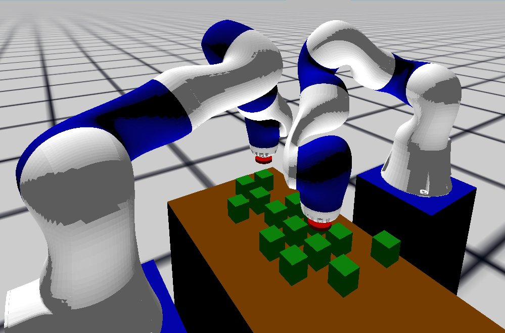
Figure 5: Picker and Manipulator trials.

This section describes the experiments performed to evaluate the algorithms in two domains shown in Fig 5: a) simple picker and b) general manipulators. In order to ensure monotonicity, the object starts and goals do not overlap. Uniform cuboidal objects simplify the grasping problem, though this is not a limitation of the methods. $50$ random experiments were limited to $300s$ of computation time. The underlying ${\tt dRRT^{*}}$ motion planner is restricted to a max of $3s$ per plan. A comparison point includes a random split method, which splits $\mathcal{O}$ at random into two subsets and chooses an arbitrary ordering. Maximum of distances cost is compared to the single arm solution [19]. Computation times and success rates are reported. The trends in both experiments show that in the single-shot versions, exhaustive and MILP tend to time-out for larger $n$. Lazy variants scale much better for all the algorithms, and in some cases increase the success ratio due to retries. TOM has much better running time than exhaustive and MILP, and producing better and more solutions than random split. Overall, the results show a) our MILP succeeds more within the time limit than exhaustive, b) TOM scales the best among all the methods, and c) the cost of solutions from TOM is close to the optimal baseline, which is around half of the single arm cost.

Simple Picker: This benchmark evaluates two disk robots hovering over a planar surface scattered with objects. The robots are only free to move around in a plane parallel to the resting plane of the objects, and the robots can pick up objects when they are directly above them. Fig 6(top) all runs up to $24$ objects succeeded for TOM. MILP scales better than exhaustive. Lazy random split succeeds in all cases (bottom). In terms of solution costs (middle) exhaustive finds the true optimal. MILP matches exhaustive and TOM is competitive. In all experiments, TOM enjoys a success rate of 100%.

General Dexterous Manipulator: The second benchmark sets up two Kuka arms across a table with objects on it. The objects are placed in the common reachable part of both arms’ workspace, and only one top-down grasping configuration is allowed for each object pose. Here (Fig 7) a larger number of motion plans tend to fail, so the single shot variants show artifacts of the randomness of ${\tt dRRT^{*}}$in their success rates. Random split performs the worst since it is unlikely to chance upon valid motion plans. Single shot exhaustive and MILP scale poorly because of expensive motion planning. Interestingly, motion planning infeasibility reduces the size of the exhaustive search tree. The solution costs (middle) substantiate benefits of the use of two arms. The computation times (bottom) again show the scalability of TOM, even compared to random split.

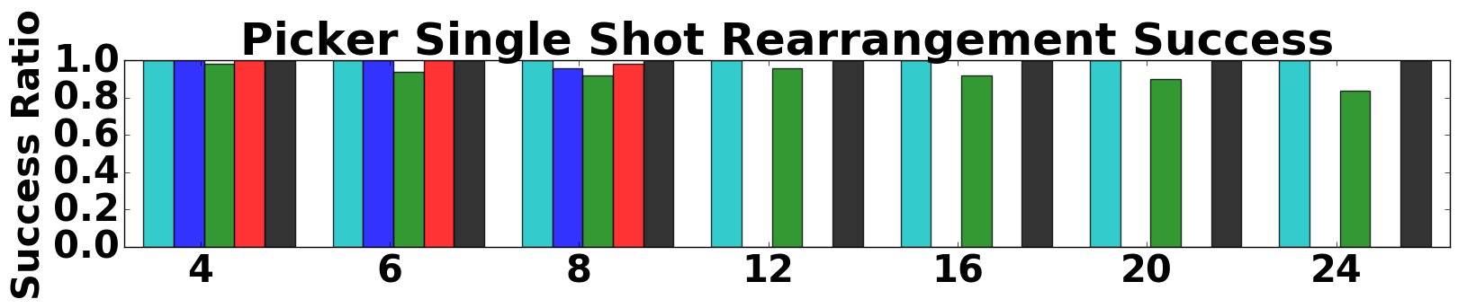
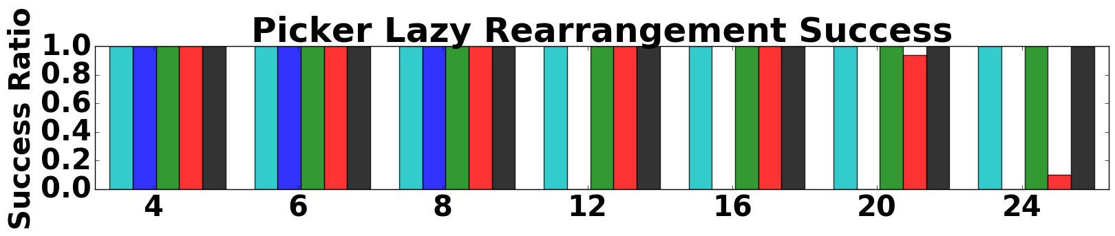
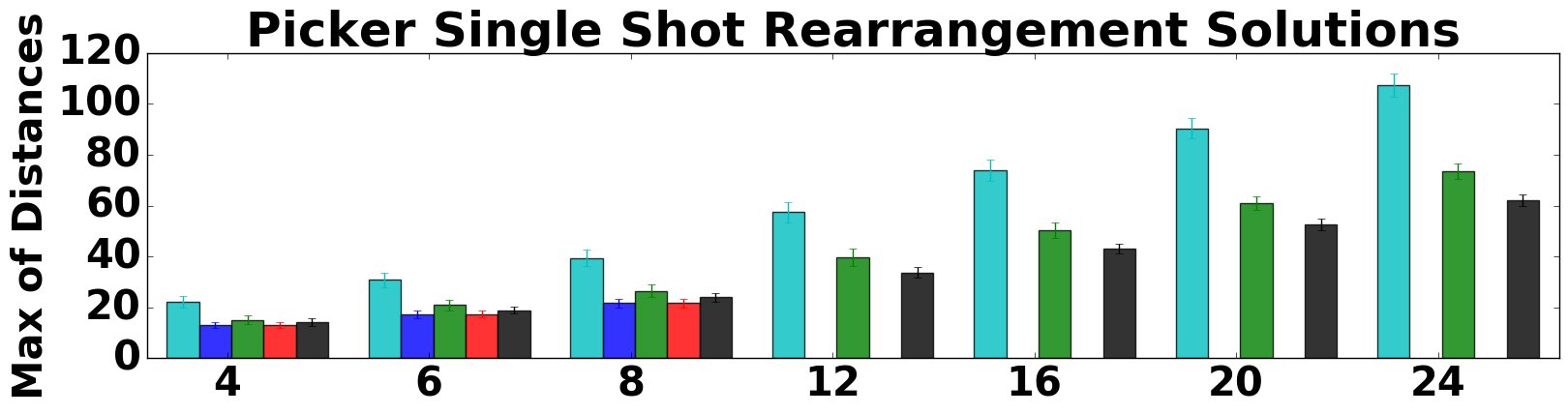
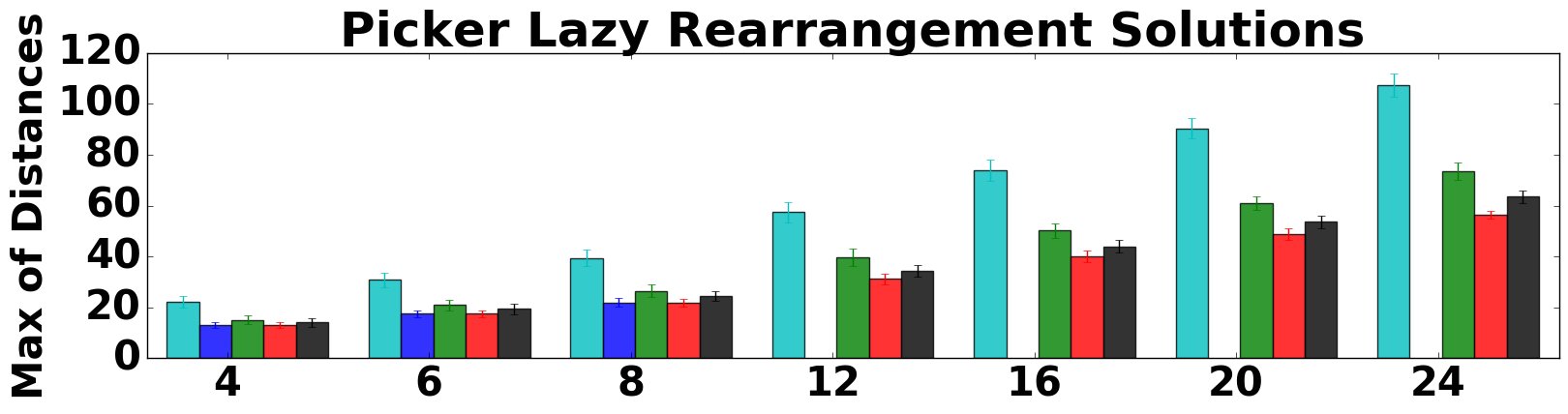
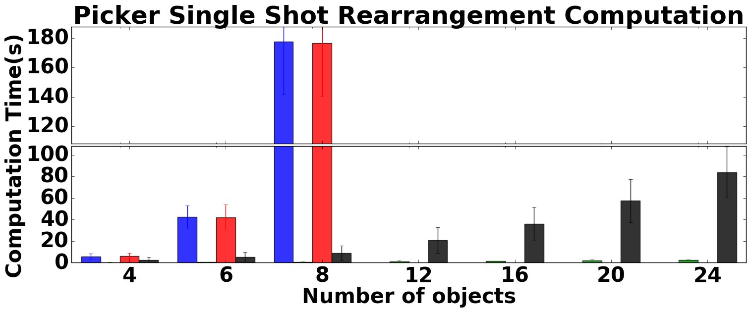
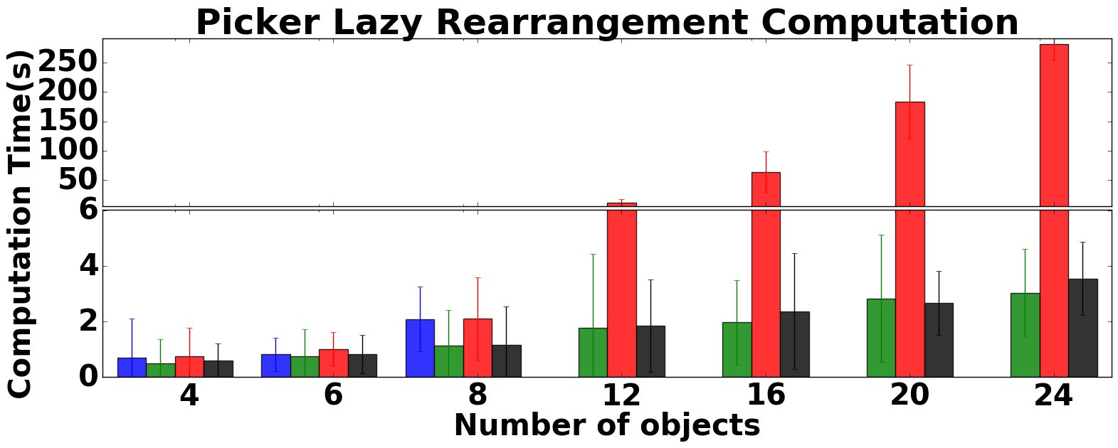
Figure 6: Simple Picker results with success(top), solution costs(middle), and computation(bottom) reported for single-shot(left) and lazy(right) versions of the methods

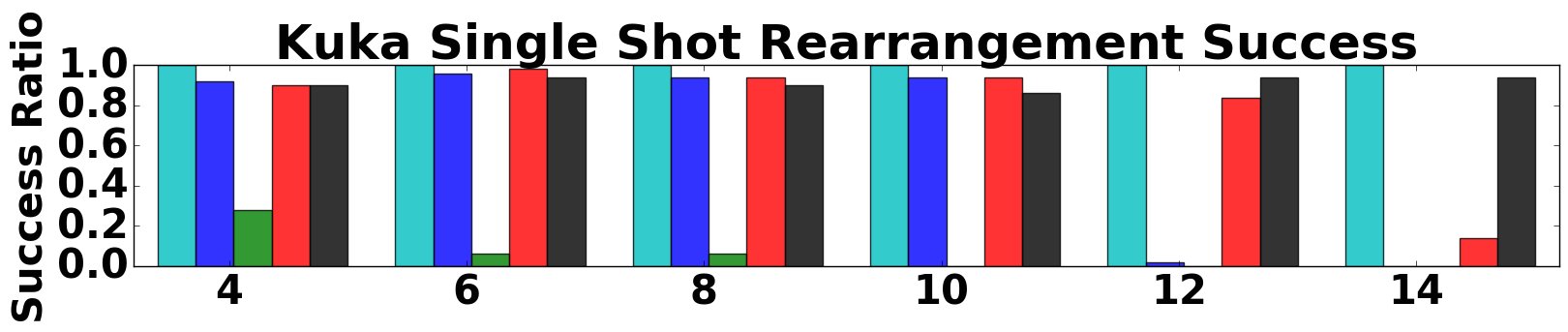
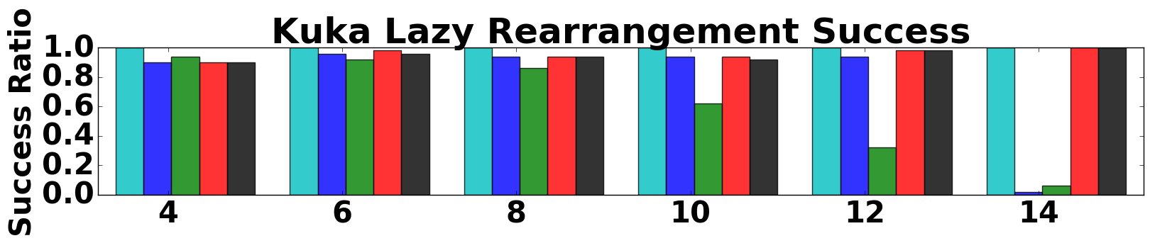
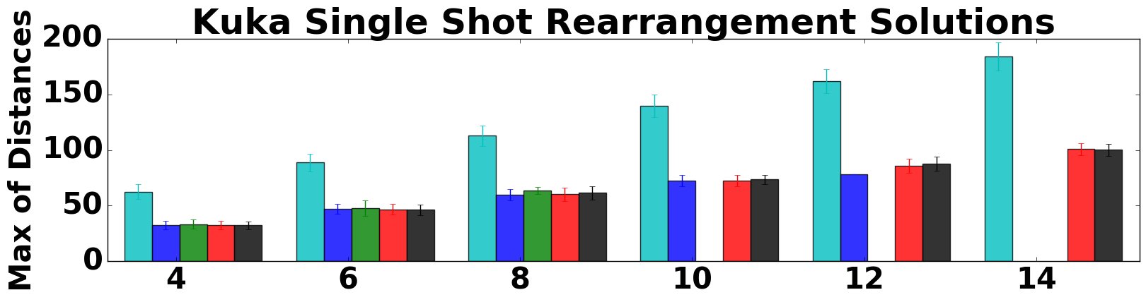
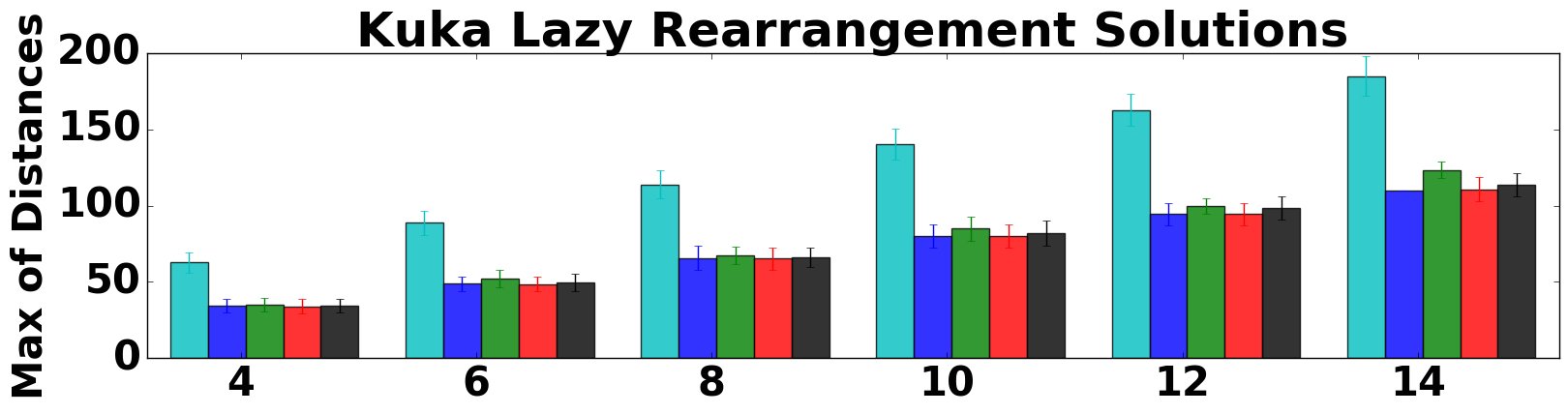
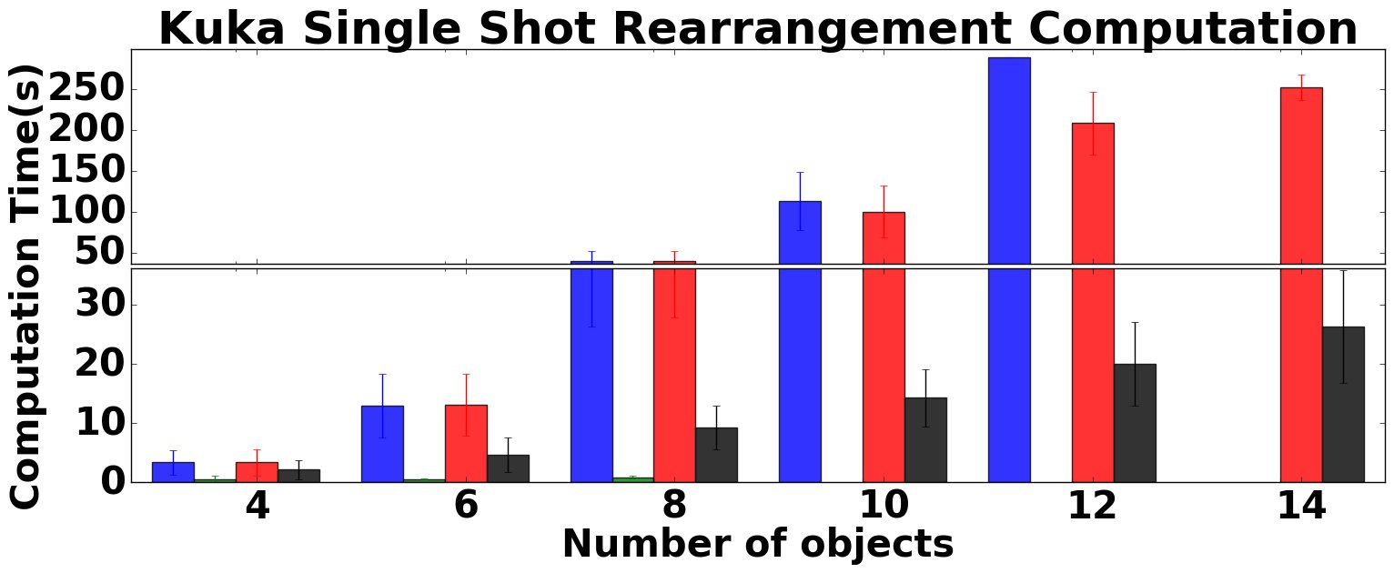
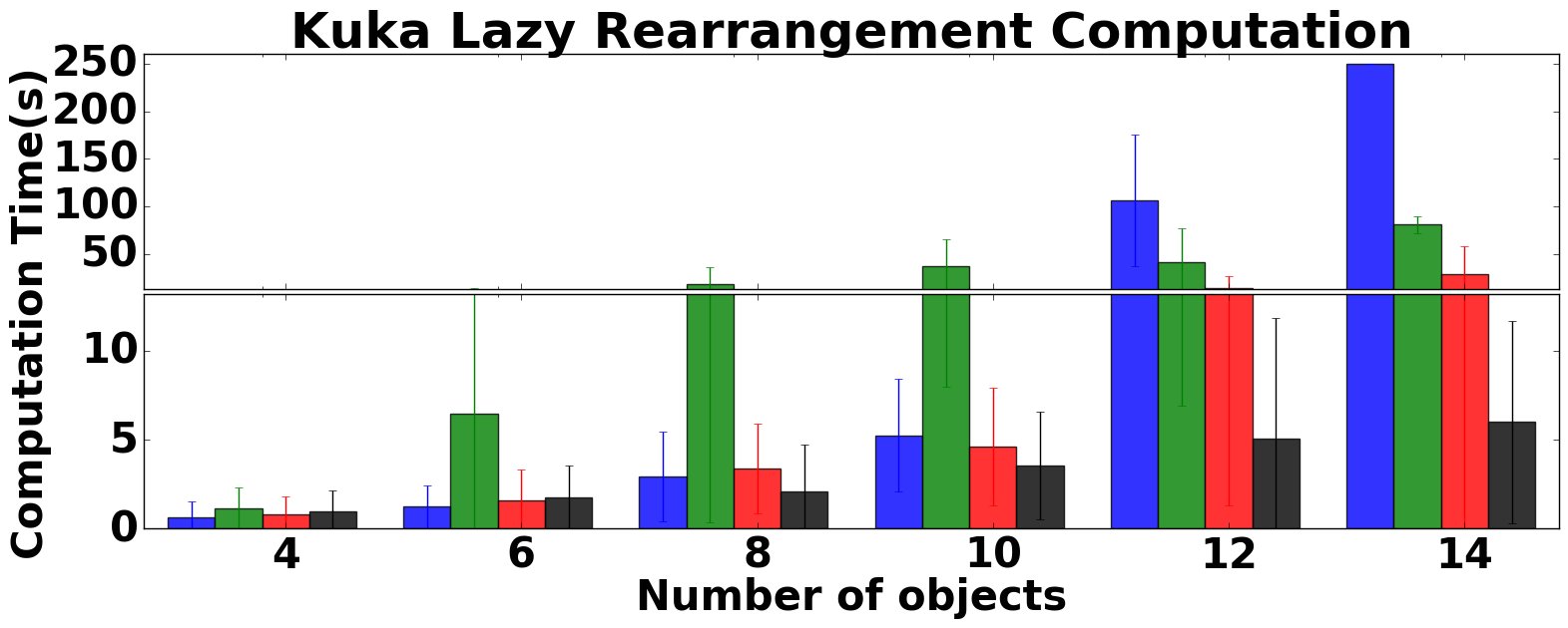
Figure 7: Kuka results with success(top), solution costs(middle), and computation(bottom) reported for single-shot(left) and lazy(right) versions of the methods

9 Discussion

The current work demonstrates the underlying structure of synchronized dual-arm rearrangement and proposes an MILP formulation, as well as a scalable algorithm TOM that provides fast, high quality solutions. Existing efficient solvers for reductions of the dual-arm problem made TOM effective. Future work will attempt to explore the $k-$arm case and instances of non-monotone rearrangement. The incorporation of manipulation and regrasp reasoning can extend these methods to more cluttered domains.

10 Appendix

10.1 Expected k-arm cost bounds in a planar disk manipulator model

The arguments made in Theorem 7.1 can be extended to $k$ disc arms. In the planar unit-square setting, with $k$ arms, there are $\frac{n}{k}$ objects for each arm to work with. Consider the transfers and transits of a set of $k$ objects, one for each arm. By [6], the arbitrary rearrangement of $k$ discs can be achieved in a bounded region with a perimeter of $O(kr)$. Clearly, the per robot additional (makespan or distance) cost is bounded by some function $f(k,r)c_{t}$, which goes to zero as $r$ goes to zero. Adding up all the potential extra cost, a $k$-arm solution has a cumulative cost

$C_{\rm k{\text{-}}arm}=C_{\rm single}+nf(k,r)c_{t}\approx(c_{pd}+0.52c_{t}+f(k,r)c_{t})n\;.$

For fixed $k$ and small $r$, $C_{\rm k{\text{-}}arm}$ is almost the same as $C_{\rm single}$. Upon considering the maximum of the two arc lengths or makespan, the $k$-arm cost becomes $C_{\rm k{\text{-}}arm}^{t}\approx(c_{pd}+0.52c_{t})\frac{n}{k}+nf(k,r)c_{t}$.

The cost ratio is

$$\frac{C_{\rm k{\text{-}}arm}^{t}}{C_{\rm single}}\approx\frac{(c_{pd}+0.52c_{t})\frac{n}{k}+nf(k,r)c_{t}}{(c_{pd}+0.52c_{t})n}=\frac{1}{k}+\frac{f(k,r)c_{t}}{c_{pd}+0.52c_{t}}\;.$$ (12)

When $r$ is small or when $\frac{c_{t}}{c_{pd}}$ is small, the $k$-arm solution is roughly $\frac{1}{k}$ as costly as the single arm solution. On the other hand, in this model a $k$-arm solution does not do better than $\frac{1}{k}$ of the single arm.

Theorem 10.1

For rearranging objects with non-overlapping starts and goals that are uniformly distributed in a unit square, a $k$-arm solution can have an asymptotic improvement of $\frac{1}{k}$ over the single arm solution.

10.2 Expected measure of the maximum of lengths of two random lines on an unit square

Prior work [16] defines the .jpg of lengths($l$) of randomly sampled lines in a rectangle of sides $a,b,\ \ a\geq b$ as

$$p(l) =(\frac{4l}{a^{2}b^{2}})\phi(l)$$

$$\phi(l) =\frac{1}{2}\pi ab-al-bl+\frac{1}{2}l^{2},\ \ l\in[0,b]$$

$$\phi(l) =ab\sin^{-1}(\frac{b}{l})+a.\sqrt[]{(l^{2}-b^{2})}-al-\frac{1}{2}b^{2},\ \ l\in[b,a]$$

$$\phi(l) =ab\{\sin^{-1}(\frac{b}{l})-\cos^{-1}(\frac{a}{l})\}+a\sqrt[]{(l^{2}-b^{2})}+b\sqrt[]{(l^{2}-a^{2})}$$

$$-\frac{1}{2}(l^{2}+a^{2}+b^{2}),\ \ l\in[a,\sqrt[]{(a^{2}+b^{2})}]$$

In the unit square model, $a=b=1$. Substituting the values, the .jpg becomes

$$p(l) =2\pi l-8\pi l^{2}+2l^{3},\ \ l\in[0,1]$$ (13)

$$p(l) =4l\sin^{-1}(\frac{1}{l})-4l\cos^{-1}(\frac{1}{l})+8l\sqrt[]{(l^{2}-1)}-2l^{3}-4l,\ \ l\in[1,\sqrt[]{2}]$$ (14)

Assuming two random sets of lines, representing transfers in a random split of objects between two arms, we need the expected value of the maximum of these pairwise lengths ie., $\mathtt{E}(max(l_{1},l_{2})),\ \ l_{1},l_{2}\ i.i.d,\ \ l_{1}\sim p,l_{2}\sim p$. This is estimated using the .jpg obtained.

$$\mathtt{E}(max(l_{1},l_{2}))=\int_{0}^{\sqrt[]{2}}\int_{0}^{\sqrt[]{2}}max(l_{1},l_{2})p(l_{1})p(l_{2})dl_{2}dl_{1}\approx 0.663$$ (15)

The result is calculated by taking into account the combination of different ranges of $p(l)$ and $max(l_{1},l_{2})$.

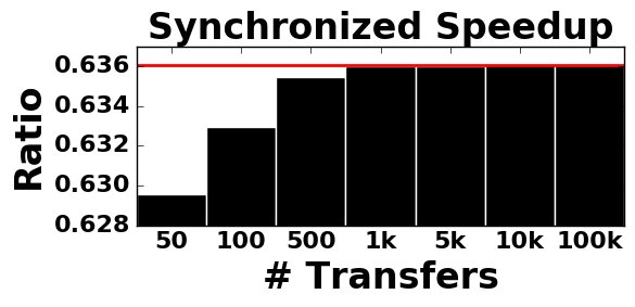
Figure 8: Empirical cost ratio versus the estimate

Prior work [29] offered an estimate for the expected length of a transit path $C_{sg}$ in terms of the expected length of a line segment, $0.52$, in a randomized setting in an unit square. With the current estimate of $0.663$ for the maximum of two such randomly sampled line segments, it follows that, the expected makespan or maximum of distances cost will use this estimate.

Using this result, the synchronized cost ratio is stated in Equation 11 as

$$\frac{C_{\rm dual}^{\rm sync}}{C_{\rm single}}\approx\frac{(c_{pd}+0.66c_{t})\frac{n}{2}+4n\pi rc_{t}}{(c_{pd}+0.52c_{t})n}$$

As a way to validate our asymptotic estimate, randomized trials were run with different number randomly sampled object transfer coordinates on an unit square. When $c_{pd}=0$ and $r=0$, the ratio of $\frac{C_{dual}^{sync}}{C_{single}}$ evaluates to $0.636$. Fig 8 verifies empirically that the ratio converges to the expected value as the number of transfers increases. This indicates the asymptotic speedup of a synchronized dual arm solution for a makespan or maximum of distances cost metric.

10.3 Smoothing

The result of the velocity tuning over the solution trajectories for the individual arms as a post-processing step is shown in Fig 9. The objective is to minimize any waits that might be a by-product of the synchronization. The small % improvements indicate that the asynchronous variants of the solutions discovered from the methods do not yield a big enough saving in execution time. Most of the improvement as a percentage of the original solution duration is not too high. On top of that, the time taken to smooth the solutions for TOM (overlaid on Fig 9) shows that it is often not beneficial. In their largest problem instances the Kuka spent $0.44s$ of smoothing time to save $3.23s$ off the solution duration, while the picker spent $9.84s$ to save $0.54s$. This indicates that among the class of synchronized solutions discovered by the proposed algorithms, the analogous asynchronous variants do not seem to be drastically better. Moreover, smoothing does not improve the maximum of distances cost measure, but only reduces the solution duration. The theoretical bounds in the simple planar setups agree with the results in that the synchronization does not degrade the benefits of using 2 arms too much. It should be pointed out though that it needs to be studied further, whether these trends would hold for a class of algorithms that can solve the asynchronous dual-arm rearrangement problem in general setups. This is out of the scope of the current work.

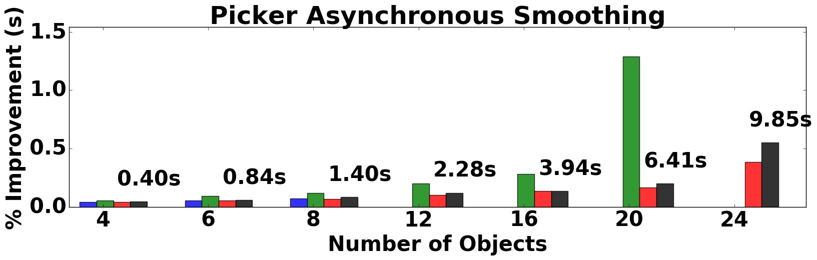
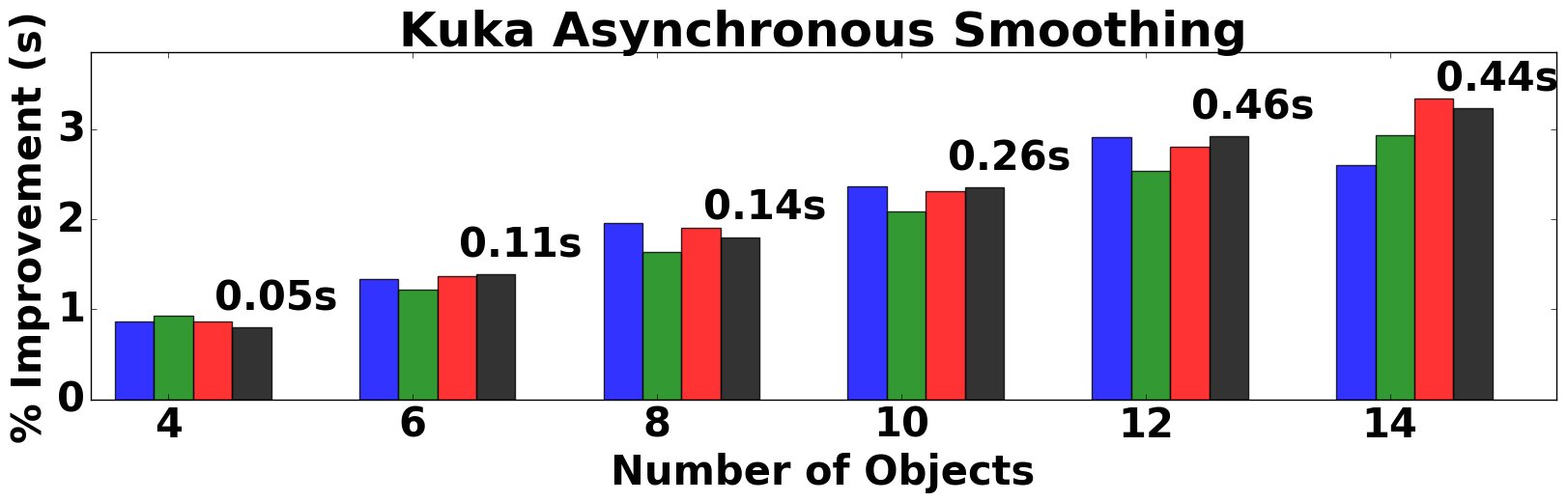
Figure 9: Smoothed solution improvement as a percentage of the original synchronized solution duration, and the time taken to smooth solutions obtained from TOM in seconds.

References

- [1] Adler, A., de Berg, M., Halperin, D., Solovey, K.: Efficient multi-robot motion planning for unlabeled discs in simple polygons. IEEE T-ASE 12(4) (2015)
- [2] Ajtai, M., Komlós, J., Tusnády, G.: On optimal matchings. Combinatorica 4(4) (1984). DOI 10.1007/BF02579135
- [3] Ben-Shahar, O., Rivlin, E.: Practical pushing planning for rearrangement tasks. IEEE Transactions on Robotics and Automation 14(4) (1998)
- [4] Berenson, D., Srinivasa, S., Kuffner, J.: Task space regions: A framework for pose-constrained manipulation planning. IJRR 30(12) (2011)
- [5] Caricato, P., Ghiani, G., Grieco, A., Guerriero, E.: Parallel tabu search for a pickup and delivery problem under track contention. Parallel Computing 29(5) (2003)
- [6] Chinta, R., Han, S.D., Yu, J.: Coordinating the motion of labeled discs with optimality guarantees under extreme density. In: WAFR (2018)
- [7] Cohen, B., Chitta, S., Likhachev, M.: Single-and dual-arm motion planning with heuristic search. IJRR 33(2) (2014)
- [8] Coltin, B.: Multi-agent pickup and delivery planning with transfers. Ph.D. thesis, Carnegie Mellon University, CMU-RI-TR-14-05 (2014)
- [9] Dezső, B., Jüttner, A., Kovács, P.: Lemon–an open source c++ graph template library. Electronic Notes in Theoretical Computer Science 264(5) (2011)
- [10] Dobson, A., Solovey, K., Shome, R., Halperin, D., Bekris, K.E.: Scalable Asymptotically-Optimal Multi-Robot Motion Planning. In: MRS (2017)
- [11] Edmonds, J.: Maximum matching and a polyhedron with 0, 1-vertices. Journal of research of the National Bureau of Standards B 69(125-130) (1965)
- [12] Frederickson, G.N., Hecht, M.S., Kim, C.E.: Approximation algorithms for some routing problems. In: FOCS (1976)
- [13] Friggstad, Z.: Multiple traveling salesmen in asymmetric metrics. In: Approximation, Randomization, and Combinatorial Optimization. Algorithms and Techniques. Springer (2013)
- [14] Galil, Z., Micali, S., Gabow, H.: An O(EV log V) algorithm for finding a maximal weighted matching in general graphs. SIAM Journal on Computing 15(1) (1986)
- [15] Gharbi, M., Cortés, J., Siméon, T.: Roadmap Composition for Multi-Arm Systems Path Planning. In: IROS (2009)
- [16] Ghosh, B.: Random distances within a rectangle and between two rectangles. Bulletin Calcutta Math Soc. 43 (1951)
- [17] Gurobi Optimization, I.: Gurobi optimizer reference manual (2016)
- [18] Halperin, D., Latombe, J.C., Wilson, R.H.: A General Framework for Assembly Planning: the Motion Space Approach. Algorithmica 26(3-4) (2000)
- [19] Han, S.D., Stiffler, N., Krontiris, A., Bekris, K., Yu, J.: Complexity results and fast methods for optimal tabletop rearrangement with overhand grasps. IJRR (2018)
- [20] Havur, G., Ozbilgin, G., Erdem, E., Patoglu, V.: Geometric rearrangement of multiple movable objects on cluttered surfaces. In: ICRA (2014)
- [21] Kirkpatrick, D., Liu, P.: Characterizing minimum-length coordinated motions for two discs. arXiv preprint arXiv:1607.04005 (2016)
- [22] Krontiris, A., Bekris, K.E.: Dealing with difficult instances of object rearrangement. In: Robotics: Science and Systems (2015)
- [23] Krontiris, A., Bekris, K.E.: Efficiently solving general rearrangement tasks: A fast extension primitive for an incremental sampling-based planner. In: ICRA (2016)
- [24] Lenstra, J.K., Kan, A.: Complexity of vehicle routing and scheduling problems. Networks 11(2) (1981)
- [25] Leroy, S., Laumond, J.P., Siméon, T.: Multiple path coordination for mobile robots: A geometric algorithm. In: IJCAI, vol. 99 (1999)
- [26] Ota, J.: Rearrangement of multiple movable objects-integration of global and local planning methodology. In: ICRA, vol. 2 (2004)
- [27] Parragh, S.N., Doerner, K.F., Hartl, R.F.: A survey on pickup and delivery models part ii: Transportation between pickup and delivery locations. Journal für Betriebswirtschaft 58(2) (2008)
- [28] Rathinam, S., Sengupta, R.: Matroid intersection and its application to a multiple depot, multiple tsp (2006)
- [29] Santaló, L.A.: Integral geometry and geometric probability. Cambridge University Press (2004)
- [30] Savelsbergh, M.W., Sol, M.: The general pickup and delivery problem. Transportation science 29(1) (1995)
- [31] Schmitt, P.S., Neubauer, W., Feiten, W., Wurm, K.M., Wichert, G.V., Burgard, W.: Optimal, sampling-based manipulation planning. In: ICRA. IEEE (2017)
- [32] Shome, R., Bekris, K.E.: Improving the scalability of asymptotically optimal motion planning for humanoid dual-arm manipulators. In: Humanoids (2017)
- [33] Solovey, K., Halperin, D.: On the hardness of unlabeled multi-robot motion planning. IJRR 35(14) (2016)
- [34] Solovey, K., Salzman, O., Halperin, D.: Finding a needle in an exponential haystack: Discrete RRT for exploration of implicit roadmaps in multi-robot motion planning. IJRR 35(5) (2016)
- [35] Solovey, K., Yu, J., Zamir, O., Halperin, D.: Motion planning for unlabeled discs with optimality guarantees. arXiv preprint arXiv:1504.05218 (2015)
- [36] Srivastava, S., Fang, E., Riano, L., Chitnis, R., Russell, S., Abbeel, P.: Combined task and motion planning through an extensible planner-independent interface layer. In: ICRA (2014)
- [37] Stilman, M., Schamburek, J.U., Kuffner, J., Asfour, T.: Manipulation planning among movable obstacles. In: ICRA (2007)
- [38] Treleaven, K., Pavone, M., Frazzoli, E.: Asymptotically optimal algorithms for one-to-one pickup and delivery problems with applications to transportation systems. IEEE Transactions on Automatic Control 59(9) (2013)
- [39] Van Den Berg, J., Stilman, M., Kuffner, J., Lin, M., Manocha, D.: Path planning among movable obstacles: a probabilistically complete approach. In: WAFR (2008)
- [40] Van Den Berg, J.P., Overmars, M.H.: Prioritized motion planning for multiple robots. In: IROS (2005)
- [41] Vega-Brown, W., Roy, N.: Asymptotically optimal planning under piecewise-analytic constraints. In: WAFR (2016)
- [42] Wagner, G., Kang, M., Choset, H.: Probabilistic path planning for multiple robots with subdimensional expansion. In: ICRA (2012)
- [43] Wilfong, G.: Motion planning in the presence of movable obstacles. Annals of Mathematics and Artificial Intelligence 3(1) (1991)
- [44] Wilson, R.H., Latombe, J.C.: Geometric Reasoning about Mechanical Assembly. Artificial Intelligence Journal 71(2) (1994)
- [45] Yu, J., Chung, S.J., Voulgaris, P.G.: Target assignment in robotic networks: Distance optimality guarantees and hierarchical strategies. IEEE Transactions on Automatic Control 60(2) (2015)
- [46] Yu, J., LaValle, S.M.: Optimal multirobot path planning on graphs: Complete algorithms and effective heuristics. IEEE Transactions on Robotics 32(5) (2016)