Novel Near-Optimal Scalar Quantizers with Exponential Decay Rate and Global Convergence

Abstract

Many modern distributed real-time signal sensing/monitoring systems require quantization for efficient signal representation. These distributed sensors often have inherent computational and energy limitations. Motivated by this concern, we propose a novel quantization scheme called approximate Lloyd-Max that is nearly-optimal. Assuming a continuous and finite support probability distribution of the source, we show that our quantizer converges to the classical Lloyd-Max quantizer with increasing bitrate. We also show that our approximate Lloyd-Max quantizer converges exponentially fast with the number of iterations. The proposed quantizer is modified to account for a relatively new quantization model which has envelope constraints, termed as the envelope quantizer. With suitable modifications we show optimality and convergence properties for the equivalent approximate envelope quantizer. We illustrate our results using extensive simulations for different finite support distributions on the source.

I Introduction

The widespread deployment of sensors for monitoring systems (such as pollution, weather) will generate gigantic amounts of (discrete) signals/data. For efficient storage and communication, data compression methods such as quantization will play a vital role. In order to account for limited computation and energy available at these sensor nodes (due to large scale of IoT devices and mobile sampling), novel quantization algorithms will be necessary.

Scalar quantization of a signal with known probability distribution is studied in the well-known works of Lloyd and Max [1, 2]. With the advent of distributed signal processing and in-network computations [3, 4, 5] in large scale sensor deployments, this (locally) optimal quantization scheme is infeasible due to limited energy, bandwidth and computational power at the terminal sensor nodes. The classical Lloyd-Max algorithm requires integral computations in the centroid (conditional mean) update step. In this work we introduce a nearly-optimal scalar quantization algorithm, known as Approximate Lloyd-Max (ALM) that bypasses these computationally complex operations. We show exponentially fast convergence of ALM to the near global optima for a class of source distributions where Lloyd-Max quantizer is globally optimal. Our algorithm uses vectorized update rules that are governed by linear transforms derived from localized mean square error optimizations.

The approximate Lloyd-Max algorithm deals with the mean square error cost function. We also consider a second cost function, known as envelope constrained mean square error quantization or shortened as envelope quantizer, which is relatively new and applicable to domains spanning, environmental monitoring, protection region database for TV whitespace and others [6]. The equivalent of ALM in this case is known as Approximate Envelope Quantizer (AEQ). We show that the AEQ scheme inherits all the properties of the ALM, by suitable modifications to accomodate the envelope constraint. The classical Lloyd-Max algorithm is known to have global convergence to a unique local minima, under certain restrictive class of cost function and the probaility distribution [7, 8]. Our algorithms give a generalized proof method to establish the global convergence for the class of continuously distributed sources on a finite support. The convergence result is hinged on the linear level update rule obtained as a result of the cost minimization in a local neighborhood. The same proof methodology applies to AEQ, where the additional envelope constraint is handled suitably through level shifting.

The main contributions of this work are summarized below.

1. Linear approximation based quantization schemes - Approximate Lloyd-Max (ALM) and Approximate Envelope Quantizer (AEQ). A vectorized algorithm termed as Alternating Between Evens and Odds (ABEO) is proposed, which performs parallel computation of all the quantization levels in each iteration.

2. Convergence of ALM and AEQ is established using linear matrix transformations and the Perron-Frobenius theory [9, 10]. We show that both the algorithms convege to a unique global minima, at exponential decay rate convergence.

3. Near optimality of the approximation based quantization scheme is analytically established.

4. Simulations on source models with finite support are performed to characterize the error vs bitrate tradeoff. Experiments also confirms the near-optimality of the quantization schemes.

Key ideas : The application of function approximations for quantizer error cost optimization forms the main theme of this work. The approximation scheme proposed here, simultaneously satisfy computational simplicity and accuracy of the quantization level computation. The level updates thus obtained, is represented as a sequence of linear (matrix) transformations that satisfy row-stochastic property. The structure of these matrices enables us to use ideas from Perron-Frobenius theory to establish global convergence of the proposed algorithms. The row-stochastic nature of the vectorized update rule also finds connections in gossip algorithms and consensus models [11, 12].

II Related Literature

Fixed rate optimal scalar quantization with known data distribution and mean square error cost function, was first studied in the independent works by Lloyd and Max [1, 2]. This iterative scheme, popularly known as the Lloyd-Max algorithm, minimizes the mean square error using alternate update of the the decision boundaries and the quantization levels. Sharma extended the Lloyd-Max method to a general class of (convex/semiconvex) distortion measures [13]. This work employs a combination of dynamic programming and fast search in order to iteratively update the quantization levels. An algorithm for quantizer design considering vector data was first introduced by Linde, Buzo and Gray [14]. Quantizer design based on a known probabilistic model or on a sequence of long training data is demonstrated here. Vector quantization follows from an efficient extension of the Lloyd-Max algorithm to higher dimensions. Another work related to vector quantization, considers predictive quantizer design hinging on tree based search methods for the class of Gauss-Markov sources [15]. Ziv proposed a variable rate universal quantizer for vector data, that achieves the optimal performance within a constant gap [16]. Other variants of high dimensional quantization using lattices and Voronoi tessellations are widely studied in mathematical literature [17, 18, 19]. Gray and Neuhoff have summarized the historical evolution of the quantization schemes, both scalar and vector cases, in their comprehensive review paper [20]. A practical approach to implement quantizers under limited computational power and memory constraints are addressed by Gersho [21]. In this respect, suboptimal and asymptotically optimal (with respect to the number of quantization levels) schemes are proposed. The computational constraints discussed here differ from the envelope constraints motivated in the current paper. In the former case the constraints are due to computational costs at higher dimension, while in this paper the constraints arise from application specific design requirements.

The convergence analysis of the Lloyd-Max algorithm is widely studied in literature. Convergence with exponential decay rate to a unique local minima, under the assumptions of a convex cost function and a log-concave probability distribution [22]. The work by Sabin and Gray explains the absolute convergence of the Lloyd algorithm and its empirical density consistency on training data [7]. The correspondence by Wu shows the convergence of the Lloyd method I for continuous, positive density function defined over a finite interval using the idea of finite state machines [8]. Another variant of this work explores dynamic programming based global optimum search methods based on the monotony properties of the error function [23]. The authors show a quadratic time algorithm that converges to the global minima. A more recent work provides a linear time accelerated multigrid search algorithm that applies to both continuous and discrete scalar probability densities [24]. Several works have studied the quantization problem in relation to the K-means clustering framework [25, 26, 27]. Pollard introduced a novel approach to show the consistency theorem for k-means cluster centers and its relation on data centric quantization. Bottou and Bengio established the optimality of the K-means algorithm using gradient descent and fast Newton algorithm [26]. High dimensional Voronoi tessellation under generalized assumptions, such as compact support are covered in some relatively recent works [17, 28].

Our contributions differ from the previous literature in the following aspects. We show an exponentially fast, globally optimal convergence result for the class of finitely supported quantizers. Also the proposed algorithm is not restricted to the class of log concave (unimodal) distributions, as assumed in many of the earlier works. Our method is analytically and computationally efficient, as it involves only the use of a sequence of linear transformations and convergence based on the Perron Frobenius theory. The proposed scheme extends to more generic cost functions and optimization constraints. This is possible since the update rules are based on local optimization of the cost function.

Notations : We use the notation, $X$ to represent a random variable and $x$ to denote the realization of the random variable. $f_{X}(x)$ represents the density function of $X$. For ease of exposition, we use the phrase ”quantization for continuous distribution” to indicate ”quantization for continuously distributed sources”.

Organization : We first develop the cost function, optimality criteria and update rule corresponding to nearly optimal quantizers, ALM and AEQ (see III). In Section IV, the main analytical result relating to the global optimality and exponential convergence of the two proposed algorithms is presented. Section V discusses the simulation experiments and convergence trends of our algorithms.

III Nearly Optimal Quantizers for Continuous Probability Distribution

This section covers the system assumptions, cost formulation, and quantizer level updates rules for the two nearly optimal quantization algorithms proposed, viz. Approximate Lloyd Max (ALM) and the Approximate Envelope Quantizer (AEQ). The cost function for ALM is based on the mean square error, while the cost function for AEQ is the envelope constraint mean square error. The two cost functions are iteratively minimized in a local neighborhood of the existing quantization levels, so as to obtain a vectorized update policy (see Sec. III-B, Sec. III-C). Sec. III-B2 provides insights into the proposed approximate quantization scheme using the example of uniformly distributed sources. We characterize the closeness of the proposed approximate schemes to their respective true (non-approximated) counterparts in an asymptotic sense, later in this section (see Sec. III-C2).

III-A Assumptions on the source distribution

Let the data observations be generated from a known continuous probability distribution $f_{X}(x)$. Without loss of generality, we assume that $f_{X}(x)$ is supported on a unit interval, $[0,1]$ . The following smoothness criterion is assumed over the slope of the distribution function:

$$\left|\frac{d}{dx}f_{X}(x)\right|<m\quad\text{ where }m\in(0,\infty).$$ (1)

The above condition states that the density function $f_{X}(x)$ has a slope bounded by $m$. A scalar quantizer is defined by a map $Q:[0,1]\rightarrow\{q_{1},q_{2},\cdots,q_{K}\}$. The image set of the map, $\{q_{1},\cdots,q_{K}\}$ represent the discrete quantization levels. For elucidating our quantization algorithm, we introduce two reference levels, $q_{0}:=0$ and $q_{K^{\prime}}:=1$, which are fixed at the endpoints of the interval $[0,1]$. In addition, we will assume the following ordering, $q_{0}\leq q_{1}\leq\cdots\leq q_{K}\leq q_{K^{\prime}}$ on the quantization levels. The parameter $K$ above, is a fixed positive integer denoting the number of quantization levels. In this paper the condition $K\gg 1$ is assumed. The subsequent discussion will elaborate on the cost functions and their minimization techniques, that lead us to the two algorithms proposed in this paper - ALM and AEQ.

III-B ALM cost minimization and level updates

The classical Lloyd-Max quantizer minimizes the mean square error (MSE) cost function, by alternating the updates between the quantization level set $\{q_{i};1\leq i\leq K\}$ and the boundary level set $\{b_{j};1\leq j\leq K+1\}$. The above minimization can be equivalently performed by minimizing a collection of local cost functions in the nearest left and right neighborhood of each quantization level. This alternative approach is used to develop the ALM algorithm. The following cost function decomposition illustrates our approach:

$$\mathcal{R}(Q): ={\mathbb{E}}\left[Q(X)-X\right]^{2}$$

$$=\int_{0}^{1}\left(Q(x)-x\right)^{2}f_{X}(x)\mbox{d}x$$

$$=\sum_{k=1}^{K}\int_{b_{k}}^{b_{k+1}}\left(q_{k}-x\right)^{2}f_{X}(x)\mbox{d}x$$ (2)

In the above equation, the boundary set $\{b_{j};1\leq j\leq K+1\}$ defined as,

$$b_{j+1} =\frac{q_{j}+q_{j+1}}{2}\quad j=1,2,\cdots,K-1,$$

$$b_{1} :=q_{0}\quad\text{ and }\quad b_{K+1}:=q_{K^{\prime}}.$$

We perform minimization of (2) by taking partial derivatives with respect to each level in the set $\{q_{i};1\leq i\leq K\}$. Using Leibniz rule of differentiation under the integral sign we get the following condition for the optimal levels [29]:

$$0=2\int_{b_{k}}^{b_{k+1}}(q_{k}-x)f_{X}(x)\mbox{d}x,$$ (3)

for $1\leq k\leq K$. The equation above, in general, does not give rise to a closed form expression for $q_{k}$. Thus, we apply a piecewise linear approximation of the density function to determine the approximate solution of (3).

III-B1 Optimal levels for approximate density

We consider the first order approximation of the density function in between the nearest neighbor quantization levels. That is,

$$f_{\mbox{\footnotesize app}}(x)=m_{k}x+c_{k},\quad\text{ for }x\in[q_{k-1},q_{k+1}]$$ (4)

where $m_{k}$ and $c_{k}$ corresponds to the slope and the intercept of the approximation. These parameters are determined using the end point conditions $f_{\mbox{\footnotesize app}}(q_{k-1})=f_{X}(q_{k-1})$ and $f_{\mbox{\footnotesize app}}(q_{k+1})=f_{X}(q_{k+1})$. The linear approximation described above helps us to obtain a computable expression for the optimal $q_{k}$ in (3). On replacing the density function $f_{X}(x)$ by its approximation $f_{\mbox{\footnotesize app}}(x)$ in the optimality condition (in (3)), a cubic equation, $r(u)=r_{0}+r_{1}u+r_{2}u^{2}+r_{3}u^{3}$ is obtained, which has a real root in the interval $[q_{k-1},q_{k+1}]$ (See Appendix B-A for the proof). For $2\leq k\leq K-1$, the equation becomes quadratic as $r_{3}=0$. The coefficients $r_{0},r_{1},r_{2}$ and $r_{3}$ are tabulated for the different quantization levels in Table. I

TABLE I: Coefficients of the cubic polynomial equation $r(u)=r_{0}+r_{1}u+r_{2}u^{2}+r_{3}u^{3}$, to determine optimal level updates of ALM

Coeff.	$k=1$	$2\leq k\leq K-1$	$k=K$
$r_{0}$	$\begin{aligned} \frac{m_{1}}{3}\left(q_{0}^{3}-\frac{q_{2}^{3}}{8}\right)+\frac{c_{1}}{2}\left(q_{0}^{2}-\frac{q_{2}^{2}}{4}\right)\end{aligned}$	$\begin{aligned} -\frac{m_{k}}{24}\left(q_{k+1}^{3}-q_{k-1}^{3}\right)-\frac{c_{k}}{8}\left(q_{k+1}^{2}-q_{k-1}^{2}\right)\end{aligned}$	$\begin{aligned} \frac{m_{K}}{3}\left(\frac{q_{K-1}^{3}}{8}-q_{K^{\prime}}^{3}\right)+\frac{c_{K}}{2}\left(\frac{q_{K-1}^{2}}{4}-q_{K^{\prime}}^{2}\right)\end{aligned}$
$r_{1}$	$\begin{aligned} -\frac{m_{1}}{2}q_{0}^{2}+\frac{c_{1}}{4}q_{2}-c_{1}q_{0}\end{aligned}$	$\begin{aligned} \frac{c_{k}}{4}\left(q_{k+1}-q_{k-1}\right)\end{aligned}$	$\begin{aligned} \frac{m_{K}}{2}q_{K^{\prime}}^{2}-\frac{c_{K}}{4}q_{K-1}+c_{K}q_{K^{\prime}}\end{aligned}$
$r_{2}$	$\begin{aligned} \frac{1}{8}m_{1}q_{2}+\frac{3}{8}c_{1}\end{aligned}$	$\begin{aligned} \frac{m_{k}}{8}\left(q_{k+1}-q_{k-1}\right)\end{aligned}$	$\begin{aligned} -\frac{1}{8}m_{K}q_{K-1}-\frac{3}{8}c_{K}\end{aligned}$
$r_{3}$	$\frac{1}{12}m_{1}$	0	$-\frac{1}{12}m_{K}$

III-B2 Insights into Approximate Lloyd-Max (ALM) quantization of uniformly distributed sources

Let us consider a continuous source having a uniform distribution in the interval $[0,1]$. The optimal mean square error (MSE) quantizer for uniform distribution is trivially obtained when the levels are fixed at equispaced locations on the unit interval. However, we draw useful insights on the ALM algorithm when the levels are initialized to random points. Starting from an initialized quantization vector $q^{\;(0)}=\left[q_{1}^{\;(0)},\cdots,q_{K}^{\;(0)}\right]$, the ALM algorithm minimizes the local cost function in the neighborhood interval, $[q_{k-1},q_{k+1}]$ of each level $q_{k}$. This results in a level update that consistently reduces the overall MSE. In this specific example of sources with uniform distribution, it is seen that the piecewise linear approximation exactly represents the true distribution. The ALM cost minimization hence follows the updates given as (see Section.III-B,III-B1),

$$b_{i+1} =\frac{q_{i}+q_{i+1}}{2}\quad\text{ for }i=1,2,\cdots,K-1$$

$$q_{i} =\frac{b_{i-1}+b_{i}}{2}\quad\text{ for }i=1,2,\cdots,K.$$ (5)

It is noted that the same updates are obtained for the Lloyd-Max algorithm. However, for general continuous distributions, the Lloyd-Max algorithm incur additional computational expense due the evaluation of an integral for the centroid update. Also, showing the global optimality of the Lloyd-Max algorithm is analytically cumbersome for a general class of probability distributions. It will be later shown that the proposed algorithm is efficient than the conventional Lloyd-Max update, since ALM gives a vectorized rule using a series of matrix products. The motivation for our vectorized method is derived from the even odd algorithm due to Maheshwari and Kumar [6]. The original method although proposed for the data driven quantizer design, extends to the model driven case that is considered in this paper. The even odd algorithm updates the quantization levels in two steps. In the first step, we modify the values of the odd set of levels, $\{q_{1},q_{3},\cdots,q_{2l+1}\}$ while keeping the even indexed levels, viz. $\{q_{2},q_{4},\cdots,q_{2m}\}$, fixed. This is followed by updating the even set, fixing the odd set. This method speeds up the computation in each iteration of the algorithm, as there are two sets of parallel update. Another advantage of the even odd algorithm is its analytical simplicity. In each level modification step, only the local neighbor points are considered. The above two properties of the even odd algorithm, helps us to represent the overall vector update as a matrix transform. For example, consider the case where $K=3$. Let $\vec{q}^{\;(0)}$ represent the (randomly) initialized quantization levels. Then the modified level after first iteration,

$$\qquad\qquad\qquad\qquad\vec{q}^{\;(1)}=P_{2}P_{1}\vec{q}^{\;(0)},$$ (6)

where

$$P_{1}=\begin{pmatrix}1&0&0&0&0\\ \frac{2}{3}&0&\frac{1}{3}&0&0\\ 0&0&1&0&0\\ 0&0&\frac{1}{3}&0&\frac{2}{3}\\ 0&0&0&0&1\end{pmatrix},\quad P_{2}=\begin{pmatrix}1&0&0&0&0\\ 0&1&0&0&0\\ 0&\frac{1}{2}&0&\frac{1}{2}&0\\ 0&0&0&1&0\\ 0&0&0&0&1\end{pmatrix}.$$

The product matrix $P_{2}P_{1}$ has the structure,

$$P=P_{2}P_{1}=\begin{pmatrix}1&0&0&0&0\\ \frac{2}{3}&0&\frac{1}{3}&0&0\\[2.84526pt] \frac{1}{3}&0&\frac{1}{3}&0&\frac{1}{3}\\[2.84526pt] 0&0&\frac{1}{3}&0&\frac{2}{3}\\ 0&0&0&0&1\end{pmatrix}.$$ (7)

The matrices $P_{1}$ and $P_{2}$ are observed to be row stochastic with non-negative entries. Hence, we can use the Perron-Frobenius theory [9, 10] to determine the fixed point of the product matrix $P_{2}P_{1}$. The fixed point determined from $P_{2}P_{1}$, corresponds the optimal solution which conforms with the optimal levels obtained using the Lloyd-Max algorithm. The above result is realized on repeated application of the update rule (6). The quantization level at the $n$-th stage is given by update, $\vec{q}^{\;(n)}=(P_{2}P_{1})^{n}\vec{q}^{\;(0)}$. As $n\rightarrow\infty$, $(P_{2}P_{1})^{n}$ converges to a rank 2 matrix with two non-zero columns. It will be later shown that these non-zero column vectors corresponds to the fixed points of $P_{2}P_{1}$. A unique optima is obtained upon imposing an ordering on the quantization levels. We show the following properties for the matrix of interest, $P$.

1. $P$ is row stochastic.

2. Eigenvalues of $P$ satisfy $|\lambda|\leq 1$.

3. $\lambda=1$ is an eigenvalue and $\mathbf{1}=[1,1,\cdots,1]^{T}$ is a corresponding eigenvector.

4. All eigenvectors of $P$ are either symmetric or antisymmetric.

5. The geometric multiplicity of $\lambda=1$ is 2; ie there are 2 eigenvectors corresponding to the eigenvalue $1$.

6. If $\vec{v}_{1}$ is an eigenvector of $\lambda=1$, then $\vec{v}_{2}=\mathbf{1}-\vec{v}_{1}$ is an independent eigenvector of $\lambda=1$.

The proof of the above results are discussed in Appendix A. Using these properties we can show that there exists a fixed point such that $\vec{q}_{\mbox{\footnotesize opt}}=\lim_{n\rightarrow\infty}\vec{q}^{\;(n)}$ and $P\vec{q}_{\mbox{\footnotesize opt}}=\vec{q}_{\mbox{\footnotesize opt}}$. The proposed method is noted for its exponential rate of convergence. For the example above, the decay rate is $O\left(\frac{1}{3^{n}}\right)$, as the second largest eigenvalue of $P$ is $\frac{1}{3}$.

For an envelope constrained uniform quantizer, the update rules are similar to the MSE quantizer, except for a level shift. In the following section we will discuss the envelope quantization algorithm for continuous probability density, based on insights derived from the quantization of uniform distributions.

III-C AEQ cost minimization and level updates

Let the mean square error cost with the envelope constraint imposed be denoted as $\mathcal{R}(Q)$. The following splitting of terms is possible on the terms of $\mathcal{R}(Q)$:

$$\mathcal{R}(Q) :={\mathbb{E}}\left[(Q(X)-X)^{2}\right]\quad\text{where }Q(X)\geq X,$$

$$=\int_{0}^{1}\left(Q(x)-x\right)^{2}f_{X}(x)\mbox{d}x\quad\text{where }Q(x)\geq x,$$

$$=\sum_{k=1}^{K}\int_{q_{k-1}}^{q_{k}}\left(q_{k}-x\right)^{2}f_{X}(x)\mbox{d}x.$$ (8)

The simplification in the cost function above is performed by substituting $Q(x)=q_{k}$ for $q_{k-1}\leq x<q_{k}$. It is observed that the total cost can be minimized with respect to the each quantization level $q_{k};\;k=1,\cdots,K$. The minima corresponds to equating the partial derivative to zero. That is,

$$0= \frac{\partial\mathcal{R}(Q)}{\partial q_{k}}$$

$$= \frac{\partial}{\partial q_{k}}\int_{q_{k-1}}^{q_{k}}(q_{k}-x)^{2}f_{X}(x)\mbox{d}x$$

$$+\frac{\partial}{\partial q_{k}}\int_{q_{k}}^{q_{k+1}}(q_{k+1}-x)^{2}f_{X}(x)\mbox{d}x$$

$$= \int_{q_{k-1}}^{q_{k}}2(q_{k}-x)f_{X}(x)\mbox{d}x-(q_{k+1}-q_{k})^{2}f_{X}(q_{k})$$ (9)

In the above equation, it is noted that corresponding to $q_{k}$, the nearest neighbor levels $q_{k-1}$ and $q_{k+1}$ are fixed. This implies that the quantizer level updates can be performed simultaneously for all even (or odd) indices, while fixing the odd (or even) indices. Since the modified quantization levels can be determined by two separate parallel updates of even and odd sets, we term this procedure as Alternating Between Evens and Odds (ABEO). This update rule will considerably speed up the proposed quantization approach. It is observed that, in general (9) does not ensure a closed-form solution of $q_{k}$. Hence we provide a linear approximation based algorithm for envelope quantization. This is considered in the next section.

III-C1 Linear Approximation Based Algorithm

The linear approximation described for ALM (in (4)) helps us to obtain a closed-form expression for the optimal $q_{k}$ for the AEQ levels. We rewrite the sufficient condition for optimality using the approximate density function $f_{\mbox{\footnotesize app}}(x)$.

$$0=\int_{q_{k-1}}^{q_{k}}2(q_{k}-x)f_{\mbox{\footnotesize app}}(x)\mbox{d}x-(q_{k+1}-q_{k})^{2}f_{\mbox{\footnotesize app}}(q_{k})$$ (10)

We substitute (4) in the above equation, to obtain a third order polynomial equation, $p(u)=p_{0}+p_{1}u+p_{2}u^{2}+p_{3}u^{3}$. The coefficients $p_{j};\;j=0,1,2,3$ depends on the nearest neighbor levels, $q_{k-1}$ and $q_{k+1}$. We list these coefficients in Table II.

TABLE II: Coefficients of the cubic polynomial equation $p(u)=p_{0}+p_{1}u+p_{2}u^{2}+p_{3}u^{3}$, to determine optimal level updates of AEQ

Coeff.	$1\leq k\leq K$
$p_{0}$	$\begin{aligned} \frac{2}{3}m_{k}q_{k-1}^{3}+c_{k}\left(q_{k-1}^{2}-q_{k+1}^{2}\right)\end{aligned}$
$p_{1}$	$\begin{aligned} -2c_{k}(q_{k-1}-q_{k+1})-m_{k}(q_{k+1}^{2}+q_{k-1}^{2})\end{aligned}$
$p_{2}$	$\begin{aligned} 2m_{k}q_{k+1}\end{aligned}$
$p_{3}$	$\begin{aligned} -\frac{2}{3}m_{k}\end{aligned}$

The roots of the cubic equation $p(u)=0$ in the interval $[q_{k-1},q_{k+1}]$, corresponds to the optimum level update of $q_{k}$. The existence of atleast one real root in $[q_{k-1},q_{k+1}]$ is shown in the Appendix B-B. The proposed linear approximation based quantization scheme is described in a step-wise manner in Algorithm. 1.

1

Input : Input distribution $f_{X}(x)$, $K=$ # of levels, MaxIter, Threshold

Output : List of quantization levels, $\vec{q}$

Initialization : $\vec{q}^{\;(0)}=\left[0,\frac{1}{K},\frac{2}{K},\cdots,1\right]$, stop condition = False, $i=0$, dist = 0

2

3while !stop condition do

4       $\mathcal{Q}_{\mbox{\footnotesize odd}}=\{q_{1},q_{3},\cdots,q_{2m+1}\}$

5       $\mathcal{Q}_{\mbox{\footnotesize even}}=\{q_{2},q_{4},\cdots,q_{2l}\}$

6              % where $\max\{2l,2m+1\}=K-1$

7       for (In Parallel) $q_{k}$ in $Q_{\mbox{\footnotesize odd}}$ do

8             $|$

9             Set linear approximation parameters :

$$\mbox{ Slope: }m_{k}=\frac{f_{X}(q_{k+1})-f_{X}(q_{k-1})}{q_{k+1}-q_{k-1}},$$

$$\mbox{ Intercept: }c_{k}=f_{X}(q_{k+1})-m_{k}q_{k+1},\text{ and }$$

$$p(u)=p_{0}+p_{1}u+p_{2}u^{2}+p_{3}u^{3}\text{ (see Table \ref{tab:AEQ_solve_cubic})}$$

$q_{k}^{(i+1)}\leftarrow\{v\in[q_{k-1},q_{k+1}]:p(v)=0\}$ $\color[rgb]{1,1,1}{1}\;\;\;\;\;\qquad\color[rgb]{0,0,0}{\text{Note:}(\mbox{Im}(r)=0\})}$

10             $|$

11       end for

12      for (In Parallel) $q_{k}$ in $\mathcal{Q}_{\mbox{\footnotesize even}}$ do

13             $|$

14             Update $q_{k}$ with steps in $\mathcal{Q}_{\mbox{\footnotesize odd}}$ loop above

15             $|$

16       end for

17      $\mbox{dist}\leftarrow\mathcal{R}(\vec{q}^{\;(i+1)})$; $\quad i\leftarrow i+1$

18      if (dist $<$ Threshold) or (iter $>$ MaxIter) then

19             stop condition = True

20       end if

21      

22 end while

Algorithm 1 Scalar Envelope Quantizer Algorithm

For the ALM scheme, the steps of Algorithm. 1 is valid, when the level modification step in line 8 is performed using the cubic polynomial $r(u)$ in Table. I instead of $p(u)$. The ALM and AEQ levels obtained using the piecewise linear approximation will be shown to be arbitrarily close to their respective true levels as $K\rightarrow\infty$.

III-C2 Asymptotic Optimality of Piecewise Linear Approximation

Let $\vec{q}^{\;\ast}(.)$ be the optimal quantizer with respect to the true density function and $\vec{q}_{\mbox{\scriptsize A}}^{\;\ast}(.)$ be the quantizer obtained by the linear approximation of the density $f_{X}(x)$. The asymptotic convergence (as quantization levels $K\rightarrow\infty$) of the linear approximation scheme can be established by using the Taylor series expansion. At $x=q_{k}$, the Taylor approximation around the interval $x\in[q_{k}-\delta/2,q_{k}+\delta/2]$ and $\delta>0$, is given by

$$f_{X}(x) =f_{X}(q_{k})+f_{X}^{\prime}(q_{k})(x-q_{k})+O((x-q_{k})^{2})$$

$$=m_{k}x+c_{k}+O\left((x-q_{k})^{2}\right)$$

$$=f_{\mbox{\footnotesize app}}(x)+O\left((x-q_{k})^{2}\right).$$ (11)

For the simplifying the notations in the analysis, we restrict our attention to the value of $k=2$. The two neighboring levels of interest are $q_{1}$ and $q_{3}$. Let $q_{2}^{\ast}$ and $q_{2\mbox{\scriptsize A}}^{\ast}$ denote the optimal level updates of the true density and the approximated density respectively (see (9) and (10)). Then, the Taylor expansion at $x=q_{2}^{\ast}$ is,

$$f_{X}(q_{2}^{\ast})=f_{\mbox{\footnotesize app}}(q_{2}^{\ast})+O(\varepsilon_{K}),$$ (12)

where $\varepsilon_{K}=\max_{1\leq k\leq K-1}|q_{k+1}-q_{k-1}|^{2}$. Using the above fact, $|q_{2}^{*}-x|^{2}\leq|q_{3}-q_{1}|^{2}\leq\varepsilon_{K}$ for all $x\in(q_{1},q_{3})$. For the specific example of a uniformly distributed source, $\varepsilon_{K}=\frac{1}{K^{2}}$. The asymptotic optimality of the ALM and AEQ schemes, as $K\rightarrow\infty$ is summarized in the following result.

Theorem 3.1 (Asymptotic optimality of ALM and AEQ).

The approximate solution of the quantization level update (see Table. I for ALM and Table. II for AEQ), $q_{2\mbox{\scriptsize A}}^{\ast}$ converges to the true solution, $q_{2}^{\ast}$ as the number of levels $K\rightarrow\infty$. That is, there exists a $K\geq K_{0}$ such that $|q_{2\mbox{\scriptsize A}}^{\ast}-q_{2}^{\ast}|\leq\varepsilon$ for all $\varepsilon>0$.

Proof.

The proofs for ALM and AEQ schemes are dealt separately below.

ALM Optimality : Consider the level update expression in (3) evaluated at the true solution $q_{2}^{\ast}$. Using the fact that $b_{2}:=\frac{q_{1}+q_{2}}{2}$, the expressions corresponding to the true density, $f_{X}(x)$ and its approximation, $f_{\mbox{\footnotesize app}}(x)$ are given by,

$$0=2\int_{b_{2}}^{b_{3}}(q_{2}^{\;\ast}-x)f_{X}(x)\mbox{d}x$$ (13)

$$D=2\int_{b_{2}}^{b_{3}}(q_{2}^{\;\ast}-x)f_{\mbox{\footnotesize app}}(x)\mbox{d}x$$ (14)

On subtracting the (13) from (14) and using the Taylor approximation in (12), we show,

$$D =\frac{1}{4}(q_{3}-q_{1})\left(q_{2}^{\;\ast}-\frac{q_{3}+q_{1}}{2}\right)O(\varepsilon_{K})$$

$$=O(\varepsilon_{K}^{2})$$ (15)

We use the fact that the local MSE cost function about $q_{2}$ is continuous and has a positive second derivative. By the continuity of the cost function, we infer that $q_{2\mbox{\scriptsize A}}^{\;\ast}\rightarrow q_{2}^{\;\ast}$ as $K\rightarrow\infty$.

AEQ Optimality : We note that the true solution $q_{2}^{\ast}$ satisfies the optimality equation in (9). On applying $q_{2}=q_{2}^{\ast}$ in (10), the rule is satisfied with an offset value $D$. That is,

$$\int_{q_{1}}^{q_{2}^{\ast}}2(q_{2}^{\ast}-x)f_{X}(x)\mbox{d}x-(q_{3}-q_{2}^{\ast})^{2}f_{X}(q_{2}^{\ast}) =0$$ (16)

$$\int_{q_{1}}^{q_{2}^{\ast}}2(q_{2}^{\ast}-x)f_{\mbox{\footnotesize app}}(x)\mbox{d}x-(q_{3}-q_{2}^{\ast})^{2}f_{\mbox{\footnotesize app}}(q_{2}^{\ast}) =D$$ (17)

Subtracting (16) from (17), we get

$$D =\int_{q_{1}}^{q_{2}^{\ast}}\left[2(q_{2}^{\ast}-x)\right]O\left(\varepsilon_{K}\right)\mbox{d}x-\left[(q_{3}-q_{2}^{\ast})^{2}\right]O\left(\varepsilon_{K}\right)$$

$$=2\left(q_{3}-q_{1}\right)\left(q_{2}^{\ast}-\frac{q_{1}+q_{3}}{2}\right)O\left(\varepsilon_{K}\right)$$

$$=O\left(\varepsilon_{K}^{2}\right)$$ (18)

The above result shows that the offset $D$ as a function of the optimal solution $q_{2}^{\ast}$ eventually converges to zero. Since the approximate solution, $q_{2\mbox{\scriptsize A}}^{\ast}$ is the root of the left hand side of (17), we argue that $q_{2\mbox{\scriptsize A}}^{\ast}$ approaches $q_{2}^{\ast}$ arbitrarily close, as $K\rightarrow\infty$. The fact is true since the AEQ optimality condition (10) is continuous in $q_{2}$ and has a positive derivative at $q_{2\mbox{\scriptsize A}}^{\ast}$ (see Appendix C for proof). The above properties ensure that, $q_{2\mbox{\scriptsize A}}^{\ast}\rightarrow q_{2}^{\ast}$ as $D\rightarrow 0$. ∎

Remark 1 (An alternate bound on ALM and AEQ near optimality result).

The absolute difference of the nearly optimal and the true optimal values of $q_{2}$ are bounded by the maximum length of the interval $[q_{k-1},q_{k+1}];\;k=1,2,\cdots,K-1$. That is,

$$|q_{2\mbox{\scriptsize A}}^{\ast}-q_{2}^{\ast}|\leq|q_{3}-q_{1}|\leq\sqrt{\varepsilon_{K}}.$$

This gives a loose bound on the near optimality, which follows directly from the decreasing interval length with $k$.

The above result holds true when $k=2$ is replaced by any $1\leq k\leq K-1$. Hence, we see that the approximated quantization vector $\vec{q}_{\mbox{\scriptsize A}}^{\;\ast}$ converges to the true quantization vector $\vec{q}^{\;\ast}$ under the $\ell_{\infty}$ norm. That is,

$$\|\vec{q}_{\mbox{\scriptsize A}}^{\;\ast}-\vec{q}^{\;\ast}\|_{\infty}:=\max_{1\leq k\leq K}|q_{k\mbox{\scriptsize A}}^{\ast}-q_{k}^{\ast}|\rightarrow 0$$

In simulations (shown in Fig. 4(g)-(i)) , it is observed that the quantization levels obtained from the approximation schemes are close to the true optima, computed using the original density function. The ALM and AEQ schemes proposed here achieves a nearly optimal solution, with a reduced computational burden.

From this point, we treat the analysis of ALM and AEQ algorithms in a common framework. We abstract out the solution of the cost minimization procedure, that is the roots of the polynomials in Table I and Table II, and express the resulting levels shifts as linear transformations.

III-D Level shifts as linear updates

The optimal solution for the iterative update of level $q_{k}$ is given by the roots of (3) or (10) in the interval $[q_{k-1},q_{k+1}]$. The solution at $i$-th iteration can be expressed as a convex combination,

$$q_{k}^{(i+1)}=\theta_{k}^{(i)}q_{k-1}^{(i)}+(1-\theta_{k}^{(i})q_{k+1}^{(i)}\quad\text{ where }\theta_{k}^{(i)}\in[0,1].$$ (19)

The above update equation will aid in the convergence analysis of the proposed algorithm. In vector notation the ABEO update rule can be expressed as,

$$\vec{q}^{\;(i+1)}=P_{\mbox{\footnotesize odd}}^{(i)}P_{\mbox{\footnotesize even}}^{(i)}\vec{q}^{\;(i)}\quad\text{ where }i=0,1,\ldots.$$ (20)

In the above equation $P_{\mbox{\footnotesize even}}^{(i)}$ and $P_{\mbox{\footnotesize odd}}^{(i)}$ are square matrices having dimension $K^{\prime}+1$. Note that for the ALM scheme $K^{\prime}=K+1$ and for AEQ $K^{\prime}=K$. These square matrices determines the optimal level updates obtained using (19). For instance, for $K^{\prime}=4$,

$$P_{\mbox{\footnotesize odd}}^{(i)} =\begin{pmatrix}1&0&0&0&0\\ \theta_{1}^{(i)}&0&1-\theta_{1}^{(i)}&0&0\\ 0&0&1&0&0\\ 0&0&\theta_{3}^{(i)}&0&1-\theta_{3}^{(i)}\\ 0&0&0&0&1\end{pmatrix},$$

$$P_{\mbox{\footnotesize even}}^{(i)} =\begin{pmatrix}1&0&0&0&0\\ 0&1&0&0&0\\ 0&\theta_{2}^{(i)}&0&1-\theta_{2}^{(i)}&0\\ 0&0&0&1&0\\ 0&0&0&0&1\end{pmatrix}.$$ (21)

We note that the two matrices, $P_{\mbox{\footnotesize odd}}$ and $P_{\mbox{\footnotesize even}}$ are row stochastic. A (row) symmetry on the location of the zeros is also observed. The matrix operators preserve the values of reference levels, $q_{0}$ and $q_{K}$ in every iteration. This is attributed to the first and the last rows of the (21) The vector update of the quantizer explained in (20)-(21), has got the required structure to apply convergence using the Perron Frobenius theory [9, 10].

IV Convergence Analysis of Near Optimal Quantizers

This section describes the analysis for convergence of the linear approximation based method in Algorithm 1. Using the fact that, the product of two row stochastic matrices is row stochastic, we show that $P^{(i)}:=P_{\mbox{\footnotesize even}}^{(i)}P_{\mbox{\footnotesize odd}}^{(i)}$ has every row that sums to unity. For the $K=4$ case, the above product matrix has the following structure:

$$P^{(i)}=\begin{pmatrix}1&0&0&0&0\\ \theta_{1}^{(i)}&0&\bar{\theta}_{1}^{(i)}&0&0\\ \theta_{2}^{(i)}\theta_{1}^{(i)}&0&\bar{\theta}_{1}^{(i)}\theta_{2}^{(i)}+\bar{\theta}_{2}^{(i)}\theta_{3}^{(i)}&0&\bar{\theta}_{2}^{(i)}\bar{\theta}_{3}^{(i)}\\ 0&0&\theta_{3}^{(i)}&0&\bar{\theta}_{3}^{(i)}\\ 0&0&0&0&1\end{pmatrix},$$ (22)

where $\bar{\theta}_{k}^{(i)}=1-\theta_{k}^{(i)}$ is used for concise notation. Other properties from the individual matrices, such as (row) symmetry on zero locations, are carried forward to the $P^{(i)}$ matrix. The first and last rows of the matrix are independent of the scale parameters $\theta_{j};\;\;j=1,\cdots,K-1$. An important observation is regarding the zero vectors, that appear alternatively in the columns of the above matrix. This occurs due to the fact that the linear updates $P_{\mbox{\footnotesize odd}}^{(i)}$ and $P_{\mbox{\footnotesize even}}^{(i)}$, acts only on the alternate entries (nearest neighbors) of the quantization vector $\vec{q}^{\;(i)}$. An important observation on $P^{(i)}$ is that $0\geq[P^{(i)}]_{l,m}\leq 1$ for all entries $(l,m)$. Further, we show that the coefficient of the linear combination $\theta_{j}^{(i)}$ for $j=1,2,\cdots,K-1$ are bounded away from the extremes $0$ and $1$. This is shown in the Fact below.

Proposition 1 ($\theta_{j}$’s are bounded away from extremes).

The coefficients $\theta_{j}^{(i)}$ for $j=1,2,\cdots,K-1$ in (22) satisfy the criteria $0<\theta_{j}^{(i)}<1$ for all iteration count $i$.

Proof.

From the smoothness assumption (1), we deduce the fact that the linear approximation slope is bounded, that is, $|m_{k}|\leq B$. First, we consider the case when $m_{k}=0$. From the ALM and AEQ optimality conditions (see (3) and (10)) we observe that $q_{k}=\frac{1}{2}q_{k-1}+\frac{1}{2}q_{k+1}$. In other words, a flat density approximation results in $\theta_{k}=\frac{1}{2}$.

In the second case, when $m_{k}\neq 0$ and $|m_{k}|\leq B$, we show that $\theta_{k}\in(0,1)$. To establish the result, we first observe the fact that the ALM and AEQ solutions always lie in the interval $[q_{k-1},q_{k+1}]$ (see Appndix B-A, B-B). Thus $\theta_{k}\in[0,1]$. We now consider the boundary cases corresponding to $\theta_{k}=0$ and $\theta_{k}=1$. These are equivalent to the solution $q_{k}=q_{k+1}$ and $q_{k}=q_{k-1}$ respectively. It is observed that under these extreme cases the ALM and AEQ optimality conditions (see (3) and (10)) are valid only when $q_{k+1}=q_{k-1}$; which corresponds to a trivial case. The resulting contradiction, hence shows that $\theta_{k}\in(0,1)$, for all bounded values of the slope $m_{k}$. ∎

In accordance with Algorithm 1, the quantization levels after $L$ iterations is $\vec{q}^{\;(L)}=\prod_{i=1}^{L}P^{(i)}\vec{q}^{\;(0)}$. We show the following convergence property of the product $\prod_{i=1}^{L}P^{(i)}$ below.

Proposition 2 (Convergence of columns of product matrix).

The odd columns $\{\vec{c}_{k}:k=3,5,\cdots,2m+1\}$ of the sequence $\prod_{i=1}^{L}P^{(i)}$ converges to zero as $L\rightarrow\infty$.

Proof.

We consider the first two terms of the product, viz. $P^{(1)}$ and $P^{(2)}$. The two matrices are row stochastic. Any element of the product $P^{(2)}P^{(1)}$ is an inner product between a row vector of $P^{(2)}$ and a column vector of $P^{(1)}$. Let $\vec{v}_{r}^{(2)}$ and $\vec{u}_{s}^{(1)}$ be the (column vector) representation of the $r$-th row of $P^{(2)}$ and the $s$-th column of $P^{(1)}$ respectively. Then, $w_{r,s}=[P^{(2)}P^{(1)}]_{r,s}$, the $(r,s)$ entry of the product $P^{(2)}P^{(1)}$, is the inner product between $\vec{v}_{r}^{(2)}$ and $\vec{u}_{s}^{(1)}$. That is, $w_{r,s}=\langle\vec{v}_{r}^{(2)},\vec{u}_{s}^{(1)}\rangle$. The following facts hold true for $\vec{v}_{r}^{(2)}$ and $\vec{u}_{s}^{(1)}$:

1. $\begin{aligned} \max_{1\leq t\leq K+1}[\vec{u}_{s}^{(1)}]_{t}<1\end{aligned}$ for every $s\neq 1$ and $n\neq K+1$. (See Proposition. 1)

2. $\mathbf{1}^{T}\vec{v}_{r}^{(2)}=1$ where $\mathbf{1}=[1,1,\cdots,1]^{T}$. This is true since $P^{(2)}$ is a row stochastic matrix.

Since the inner product $w_{r,s}$ is a (non-zero) convex combination (from (F2) and due to Proposition. 1) of components of $\vec{u}_{s}^{(1)}$, from (F1) we assert that

$$0\leq w_{r,s}<\max_{1\leq t\leq K+1}[\vec{u}_{s}^{(1)}]_{t}.$$ (23)

In other words, all the elements of columns $\{c_{k}:k=3,5,\cdots,2l+1\}$ are strictly less than the maximum element in the corresponding columns of $P^{(1)}$. Alternatively, we can represent this as a contraction, $\begin{aligned} w_{r,s}=\alpha\max_{t}[\vec{u}_{s}^{(1)}]_{t}\end{aligned}$, where $\alpha<1$. Using the fact that product $P^{(2)}P^{(1)}$ is row stochastic, we can extend the same argument to the product of three matrices, that is $P^{(3)}[P^{(2)}P^{(1)}]$. We make use of an induction argument to show the property in the limiting case. Let $w_{r,s}^{(n)}$ be the $(r,s)$-th element of the product matrix $\prod_{i=1}^{n}P^{(i)}$. Then using (23), we have the contraction of the sequence,

$$w_{r,s}^{(n)}=\left(\prod_{i=1}^{n}\alpha_{i}\right)\max_{1\leq s\leq K+1}w_{r,s}^{(1)},$$ (24)

where $\alpha_{i}<1$. From above we observe that, the sequence of inner product terms, $\{w_{r,s}^{(i)}:0\leq i<\infty\}$ is a monotonically decreasing sequence for every $1\leq r\leq K+1$ and $s=3,5,\cdots,2l+1$. Using monotone convergence theorem [30] on the above (bounded) sequence, we show that the columns $\vec{c}_{3},\vec{c}_{5},\cdots,\vec{c}_{2l+1}$ of the product sequence $\prod_{i=1}^{L}P^{(i)}$ eventually decreases to zero. ∎

Theorem 4.1 (Convergence to global minima).

The iteration in Algorithm. 1 converges to a quantization vector,

$$\vec{q}^{\;\ast}=P^{\ast}\vec{q}^{\;(0)},$$ (25)

where $P^{\ast}=\lim_{L\rightarrow\infty}\prod_{i=1}^{L}P^{(i)}$, and $\vec{q}^{\ast}$ is independent of the initialization $q^{(0)}$ (except for the reference levels).

Proof.

We note that the limiting product matrix $P^{\ast}=\lim_{L\rightarrow\infty}\prod_{i=1}^{L}P^{(i)}$ converges to a matrix with columns $\vec{c}_{2}=\vec{c}_{3}=\cdots=\vec{c}_{K}=\mathbf{0}$ (See Proposition. 2). The first and last columns, viz. $\vec{c}_{1}$ and $\vec{c}_{K+1}$, are non-zero vectors, as the matrix transformation $P^{(i)}$, preserves the reference levels $q_{0}$ and $q_{K}$. The structure of $P^{\ast}$ is as follows:

$$P^{\ast}=\begin{pmatrix}\kern 6.00006pt\vline&\kern 6.00006pt\vline&\cdots&\kern 6.00006pt\vline&\kern 6.00006pt\vline\\ \vec{c}_{1}&0&\cdots&0&\vec{c}_{K+1}\\ \kern 6.00006pt\vline&\kern 6.00006pt\vline&\cdots&\kern 6.00006pt\vline&\kern 6.00006pt\vline\end{pmatrix}$$ (26)

Recalling the fact that $P^{\ast}$ is a row stochastic matrix, the all ones vector $\mathbf{1}$, is an eigenvector of $P^{\ast}$ corresponding to eigenvalue $\lambda=1$. Due to this fact, we can show $\vec{c}_{1}+\vec{c}_{K+1}=\mathbf{1}$. In other words, the elements of $\vec{c}_{1}$ and $\vec{c}_{K+1}$ forms a convex combination pair. From the above fact, we also infer that, $\vec{c}_{K+1}$ is order reversed with respect to vector $\vec{c}_{1}$. The above two column vectors are also linearly independent and correspond to the eigenvectors of $\lambda=1$. Using the Gauss elimination method, we can establish that the matrix $P^{\ast}$ has a rank of 2. Since there is a repeated eigenvalue $\lambda=1$ with geometric multiplicity 2, all the remaining eigenvalues of the limiting matrix are zero. Hence, $P^{\ast}$ has two fixed points $\vec{c}_{1}$ and $\vec{c}_{K+1}$.

On imposing an order constraint on the quantization levels $0:=q_{0}\leq q_{1}\leq\cdots\leq q_{K}:=1$, we can show that $\vec{c}_{K+1}$ corresponds to the global minimizer of the Algorithm.1. The above iterative scheme has an exponential rate of convergence, as all the eigenvalues of the transform matrix $P^{(i)}$ satisfy the property that absolute value of eigenvalues atmost 1.

The initialization $\vec{q}^{\;(0)}$ (assuming $q_{0}^{(0)}=0$ and $q_{K}^{(0)}=1$), has no effect on the fixed point of $P^{\ast}$, as all the intermediate columns of the limiting matrix are zero vectors. However, the transient terms of the product $\prod_{i=1}^{L}P^{(i)}$, will depend on the initialized quantization levels for small values of $L$. ∎

Remark 2 (Uniqueness of solution).

The optimal quantization vector given by Algorithm. 1 is unique upto an ordering.

Remark 3 (Exponential rate of convergence).

The linear approximation based algorithm (see Algorithm. 1) achieves exponential rate of convergence, that is, the $\ell_{2}$ gap between the linear approximation solution and the true solution drops at a rate $O(\lambda_{(2)}^{n})$, where $\lambda_{(2)}$ represents the second largest eigenvalue of the transform matrix, $P^{(i)}$.

V Simulation Results and Discussion

We present the simulation results of the model based scalar quantization in this section. The results corresponds to finite support distributions in the interval $[0,1]$. All simulations were performed using Numpy module in Python 3.5 kernel with normal computing hardware (Intel i7, 2.2 GHz processor, 8GB RAM). We study the variations of the MSE with different simulation parameters for the unconstrained and constrained cases (see Fig. 4). The density functions considered in the simulation include the Beta distribution, truncated normal and truncated exponential distributions.

The quantizer evolution plot for the envelope quantizer on the Beta(2,4) is shown in Fig. 1. The simulation considers $K=8$ levels, with an equi-spaced initialization. The levels are seen to shift towards the peak near $x=0.25$, in a asymmetric manner. The reference levels at $x=0$ and $x=1$ are unchanged during the iteration of algorithm. The levels obtained by this linear approximation algorithm are observed to be close to optimal levels without the approximation. In Fig. 4 (a), a comparison of MSE variation for the envelope quantizer and the unconstrained quantizer is shown. The convergence of the iterative algorithm is shown in Fig. 4(b) for different values of $K$. It is noted that the convergence for each of the plots happens in approximately $K$ iterations. Fig. 4(c) describes the MSE performance of the algorithm for different symmetric Beta distributions. The MSE decays at exponential rate with the number of quantization levels. The advantage of using linear approximation scheme is shown in Fig. 4(d), by comparing the simulation time required to run the quantization algorithm. In this experiment we used the stopping criteria for the algorithm to be the iteration until the computed MSE is within $1\%$ of the optimal MSE. We observe that the ALM has an average of $3.4$x improvement with respect to the simulation time (using Beta(4,2) distribution). Fig. 4(e)-(f) shows the MSE variation of the envelope quantizer for different truncated distributions and asymmetric Beta distributions respectively. In Fig. 4(g)-(i), the quantization levels for the different MSE cost metrics is compared. It is observed that the linear approximation method closely tracks the optimal levels obtained without using the approximation. The difference between the unconstrained MSE and the envelope quantizer is explained by the quantization levels shown in Fig. 4(g) and (h). For the Beta(2,2) distribution, the unconstrained quantizer results in a symmetric set of quantization levels, while the envelope quantizer has a right shifted and asymmetric set of levels. For the asymmetric Beta(2,4) distribution, the envelope quantizer allots more number of levels around the region where the density $f_{X}(x)$ peaks (see Fig. 4(i)).

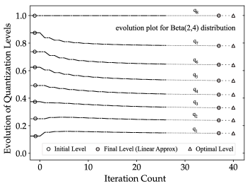
Figure 1: Evolution of quantization levels for the Beta distribution with parameters $\alpha=2$ and $\beta=4$ with a equi-spaced initialization. The plot shows the level update according to the Alternating Between Even and Odds (ABEO) algorithm. The final levels due to the linear approximation method are comparable to the optimal (true) levels computed without the approximation.

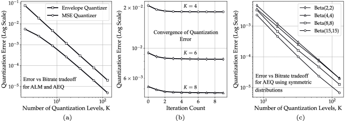
Figure 2: (a) Quantization error performance with the number of quantization levels, $K$ for Approximate Envelope Quantizer (AEQ) and Approximate Lloyd-Max (ALM). (b) Convergence of AEQ (see Algorithm. 1) with the increasing number of iterations. (c) MSE for envelope quantizer vs number of levels $K$, plotted for various symmetric Beta distributions.

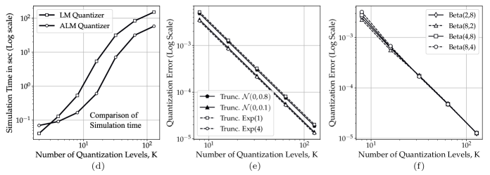
Figure 3: (d) Simulation time for compared for Lloyd-Max quantizer for two cases - with linear approximation and without linear approximation. (e) MSE and bitrate tradeoff for AEQ for different truncated distributions. (f) Variation of MSE for envelope quantizer for different asymmetric Beta distributions.

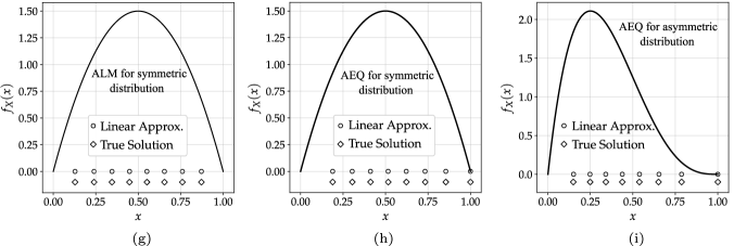
Figure 4: (g) Optimal and Near optimal (that is ALM) quantization levels for Lloyd-Max quantizer on Beta(2,2) distribution.(h) Optimal and Near optimal (that is AEQ) quantization levels for envelope quantizer on Beta(2,2) distribution. (i) Comparison of AEQ near optimal scheme with the ground truth optima for the asymmetric Beta(2,4) distribution.

VI Conclusions

We have introduced two novel methods for scalar quantization of sources with a known probability distribution on a finite support. The first quantizer, termed as ALM, effficiently determines the quantization level updates for the mean square error cost function. While the second, known as AEQ, is a relatively new quantization approach, that minimizes an envelope constrained cost function. A piecewise linear approximation method has been employed here, that significantly reduces the computational cost of the quantizer. A novel parallel update rule known as the ABEO, assists in efficiently computing the quantizer levels in a vectorized manner. Both our quantization algorithms has been shown to converge at exponential rate to the unique global minimizer of the cost function. This convergence result, which is a key contribution of this work, has its roots in the row-stochastic property associated with the quantization level update matrices. Simulation results have shown the validity of our analytical results.

Appendix A Proof of properties 1-6 for uniform quantization

Proof: 1) Since $P_{1}$ and $P_{2}$ are row stochastic, for a fixed $i$

$$\sum_{j}[P]_{ij} =\sum_{j}[P_{2}P_{1}]_{ij}$$

$$=\sum_{j}\sum_{k}[P_{2}]_{ik}[P_{1}]_{kj}$$

$$=\sum_{k}[P_{2}]_{ik}\sum[P_{1}]_{kj}$$

$$=\sum_{k}[P_{2}]_{ik}\times 1=1$$ (27)

This shows $P$ is row stochastic.

2) Consider a vector $\vec{v}$, and

$$|P\vec{v}|_{1}\leq\|P\|_{1}\|v\|_{1}$$ (28)

Since $\|P\|_{1}=1$, for all eigenvalues $|\lambda|\leq 1$.

3) Follows from 1).

4) $P$ is row symmetric in a cyclic sense, ie $\vec{r}_{i}=\text{Flip}(\vec{r}_{n-i+1})$. This follows from row symmetry of individual matrices $P_{1}$ and $P_{2}$. For a row symmetric matrix the eigenvectors satisfy,

$$P\vec{v}=\begin{bmatrix}P_{u}\\ P_{l}\end{bmatrix}\begin{bmatrix}\vec{v}_{u}\\ \vec{v}_{l}\end{bmatrix} =\lambda\begin{bmatrix}\vec{v}_{u}\\ \vec{v}_{l}\end{bmatrix}$$ (29)

$$P_{u}\begin{bmatrix}\vec{v}_{u}\\ 0\end{bmatrix}=\lambda\begin{bmatrix}\vec{v}_{u}\\ 0\end{bmatrix},\quad P_{l}\begin{bmatrix}0\\ \vec{v}_{l}\end{bmatrix} =\lambda\begin{bmatrix}0\\ \vec{v}_{l}\end{bmatrix}$$ (30)

By solving the above equations we get $\vec{v}_{u}=\vec{v}_{l}$ or $\vec{v}_{u}=-\vec{v}_{l}$.

5) We show that $P-I$ has kernel dimension (or nullity) of $2$. We observe that the diagonal element $[P-I]_{ii}=0$ for $i=2,3,\cdots,n-1$. And using the fact that each row is shifted with a preceding zero. One can show that all rows are independent except for the first and the last row. This shows that the geometric multiplicity is $2$.

6) This follows from 3) and 5).

Appendix B Existence of a real root for the linear approximation

B-A Roots corresponding to ALM

We observe that the piecewise linear approximation on the density function results in the cubic polynomial as described in Table I. Here we show that there always exists a real root for the polynomial in the interval $[q_{k-1},q_{k+1}]$. The method employed here uses the fact that a sign change in the polynomial evaluated between any two points indicates a root between them. This result is known as the intermediate value theorem. We demonstrate the steps in the proof, by determining the value of $r(u)=r_{0}+r_{1}u+r_{2}u^{2}+r_{3}u^{3}$ for each of the end points.

Case 1: $2\leq k\leq K-1$. (Here we note that $r_{3}=0$)

$$r(q_{k-1}) =r_{0}+r_{1}q_{k-1}+r_{2}q_{k-1}^{2}$$

$$=-\frac{1}{8}(q_{k+1}-q_{k-1})^{2}\left[m_{k}\left(\frac{2}{3}q_{k-1}+\frac{1}{3}q_{k+1}\right)+c\right]$$

$$=-\frac{1}{8}(q_{k+1}-q_{k-1})^{2}\left[\frac{2}{3}f_{X}(q_{k-1})+\frac{1}{3}f_{X}(q_{k+1})\right]$$

$$<0$$ (31)

At the right boundary, that is, $u=q_{k+1}$,

$$r(q_{k+1}) =r_{0}+r_{1}q_{k+1}+r_{2}q_{k+1}^{2}$$

$$=\frac{1}{8}(q_{k+1}-q_{k-1})^{2}\left[\frac{2}{3}f_{X}(q_{k+1})+\frac{1}{3}f_{X}(q_{k-1})\right]$$

$$>0$$ (32)

Case 2: $k=1$ or $K$. We show the proof for $K=1$ and explain the modifications necessary for $k=K$. The polynomial $r(u)$ evaluated at $u=q_{0}$ and $u=q_{2}$ simplifies to :

$$r(q_{0}) =-\frac{1}{2}(q_{2}-q_{0})^{2}\left[\frac{1}{3}f_{X}(q_{2})+\frac{2}{3}f_{X}(q_{0})\right]$$

$$<0$$ (33)

$$r(q_{2}) =\frac{1}{2}(q_{2}-q_{0})^{2}\left[\frac{2}{3}f_{X}(q_{2})+\frac{1}{3}f_{X}(q_{0})\right]$$

$$>0.$$ (34)

For the cubic polynomial corresponding to $k=K$, we note that all signs are reversed with respect to the $k=1$ case. The modified polynomial still evaluates to give the change in signs at the end points, that is $r(q_{K-1})<0$ and $r(q_{K^{\prime}})>0$.

B-B Roots corresponding to AEQ

We show that the polynomial equation $p(u)=p_{0}+p_{1}u+p_{2}u^{2}+p_{3}u^{3}=0$, with coefficients as listed in Table. II, has atleast one real root in the interval $[q_{k-1},q_{k+1}]$. Recall that $q_{k-1}$ and $q_{k+1}$ represents the left and right nearest neighbors of the quantization level $q_{k}$. We show the above fact using the intermediate value theorem, that is, $p(u)=0$ if $p(q_{k-1})p(q_{k+1})<0$. Evaluating the polynomial at the end points of the interval we get,

$$p(q_{k-1}) =p_{0}+p_{1}q_{k-1}+p_{2}q_{k-1}^{2}+p_{3}q_{k-1}^{3}$$

$$=-c_{k}q_{k-1}^{2}-c_{k}q_{k+1}^{2}+2c_{k}q_{k-1}q_{k+1}$$

$$\;\;\;\;-m_{k}q_{k-1}^{3}-m_{k}q_{k-1}q_{k+1}^{2}+2m_{k}q_{k-1}^{2}q_{k+1}$$

$$=-(c_{k}+m_{k}q_{k-1})(q_{k+1}-q_{k-1})^{2}$$

$$=-f_{X}(q_{k-1})(q_{k+1}-q_{k-1})^{2}$$

$$<0,$$ (35)

and

$$p(q_{k+1}) =p_{0}+p_{1}q_{k-1}+p_{2}q_{k-1}^{2}+p_{3}q_{k-1}^{3}$$

$$=c_{k}q_{k-1}^{2}+c_{k}q_{k+1}^{2}-2c_{k}q_{k-1}q_{k+1}$$

$$\;\;\;\;+\frac{2}{3}m_{k}q_{k-1}^{3}+\frac{1}{3}m_{k}q_{k+1}^{3}-m_{k}q_{k-1}^{2}q_{k+1}$$

$$=-p(q_{k-1})+\frac{1}{3}m_{k}(q_{k+1}^{3}-q_{k-1}^{3})$$

$$\;\;\;\;-m_{k}q_{k+1}q_{k-1}(q_{k+1}-q_{k-1})$$

$$=(\frac{2}{3}f_{X}(q_{k-1})+\frac{1}{3}f_{X}(q_{k+1}))(q_{k+1}-q_{k-1})^{2}$$

$$>0.$$ (36)

From the above two inequalities we observe that the product $p(q_{k-1})p(q_{k+1}))$ is always negative and hence there always exist a root of $p(u)=0$ in the interval $[q_{k-1},q_{k+1}]$.

Appendix C Proof that AEQ optimality condition results in a positive derivative

In this section we show that the AEQ optimality condition defined by the polynomial $p(u)$, in Table. II has a positive slope. The proof for the same follows from the convexity of the cost function (8). The derivative of the polynomial $p(q_{k})$ with respect to $q_{k}$ is given as,

$$\frac{dp(q_{k})}{dq_{k}} =2(q_{k+1}-q_{k-1})\left(m_{k}\left(\frac{q_{k+1}+q_{k-1}}{2}\right)+c_{k}\right)$$

$$\qquad\qquad-2m_{k}(q_{k+1}-q_{k})^{2}$$

$$=2(q_{k+1}-q_{k-1})f_{\mbox{\footnotesize app}}\left(\frac{q_{k+1}+q_{k-1}}{2}\right)$$

$$\qquad\qquad-2m_{k}(q_{k+1}-q_{k})^{2}$$ (37)

We consider the following three cases - $m_{k}=0$, $m_{k}<0$ and $m_{k}>0$. In the first and second case, we see that the derivative is positive since $f_{\mbox{\footnotesize app}}\left(\frac{q_{k+1}+q_{k-1}}{2}\right)>0$. When $m_{k}>0$, we use the fact that, the optimal solution $q_{k}$ is closer to $q_{k+1}$ than $q_{k-1}$. In other words, we get the condition $q_{k+1}-q_{k}\leq q_{k}-q_{k-1}$. Using the above fact, we rewrite (37) as,

$$\frac{dp(q_{k})}{dq_{k}} \geq 2(q_{k+1}-q_{k-1})\left[m_{k}\left(\frac{2q_{k}-q_{k+1}+q_{k-1}}{2}\right)+c_{k}\right]$$

$$\geq 2(q_{k+1}-q_{k-1})f_{\mbox{\footnotesize app}}(q_{k-1})>0$$ (38)

References

- [1] S. Lloyd, “Least squares quantization in PCM,” IEEE Transactions on Information Theory, vol. 28, no. 2, pp. 129–137, March 1982.
- [2] J. Max, “Quantizing for minimum distortion,” IRE Transactions on Information Theory, vol. 6, no. 1, pp. 7–12, March 1960.
- [3] J. B. Predd, S. B. Kulkarni, and H. V. Poor, “Distributed learning in wireless sensor networks,” IEEE Signal Processing Magazine, vol. 23, no. 4, pp. 56–69, July 2006.
- [4] A. G. Dimakis, S. Kar, J. M. F. Moura, M. G. Rabbat, and A. Scaglione, “Gossip algorithms for distributed signal processing,” Proceedings of the IEEE, vol. 98, no. 11, pp. 1847–1864, Nov 2010.
- [5] P. Vyavahare, N. Limaye, and D. Manjunath, “Optimal embedding of functions for in-network computation: Complexity analysis and algorithms,” IEEE/ACM Transactions on Networking, vol. 24, no. 4, pp. 2019–2032, Aug 2016.
- [6] G. Maheshwari and A. Kumar, “Optimal quantization of tv white space regions for a broadcast based geolocation database,” in 2016 24th European Signal Processing Conference (EUSIPCO), Aug 2016, pp. 418–422.
- [7] M. Sabin and R. Gray, “Global convergence and empirical consistency of the generalized Lloyd algorithm,” IEEE Transactions on Information Theory, vol. 32, no. 2, pp. 148–155, Mar 1986.
- [8] X. Wu, “On convergence of lloyd’s method i,” IEEE Transactions on Information Theory, vol. 38, no. 1, pp. 171–174, Jan 1992.
- [9] S. U. Pillai, T. Suel, and S. Cha, “The perron-frobenius theorem: some of its applications,” IEEE Signal Processing Magazine, vol. 22, no. 2, pp. 62–75, March 2005.
- [10] R. G. Gallager, Discrete stochastic processes. Springer Science & Business Media, 2012, vol. 321.
- [11] D. Shah et al., “Gossip algorithms,” Foundations and Trends® in Networking, vol. 3, no. 1, pp. 1–125, 2009.
- [12] M. Huang, “Stochastic approximation for consensus: A new approach via ergodic backward products,” IEEE Transactions on Automatic Control, vol. 57, no. 12, pp. 2994–3008, Dec 2012.
- [13] D. Sharma, “Design of absolutely optimal quantizers for a wide class of distortion measures,” IEEE Transactions on Information Theory, vol. 24, no. 6, pp. 693–702, November 1978.
- [14] Y. Linde, A. Buzo, and R. Gray, “An Algorithm for Vector Quantizer Design,” IEEE Transactions on Communications, vol. 28, no. 1, pp. 84–95, Jan 1980.
- [15] R. Gray and Y. Linde, “Vector quantizers and predictive quantizers for gauss-markov sources,” IEEE Transactions on Communications, vol. 30, no. 2, pp. 381–389, Feb 1982.
- [16] J. Ziv, “On universal quantization,” IEEE Transactions on Information Theory, vol. 31, no. 3, pp. 344–347, May 1985.
- [17] Q. Du, M. Emelianenko, and L. Ju, “Convergence of the Lloyd Algorithm for Computing Centroidal Voronoi Tessellations,” SIAM Journal on Numerical Analysis, vol. 44, no. 1, pp. 102–119, 2006. [Online]. Available: https://doi.org/10.1137/040617364
- [18] J. Conway and N. Sloane, “Voronoi regions of lattices, second moments of polytopes, and quantization,” IEEE Transactions on Information Theory, vol. 28, no. 2, pp. 211–226, March 1982.
- [19] J. H. Conway and N. J. A. Sloane, Sphere Packing, Lattices and Groups. NY, USA: Springer-Verlag, 1998.
- [20] R. M. Gray and D. L. Neuhoff, “Quantization,” IEEE Transactions on Information Theory, vol. 44, no. 6, pp. 2325–2383, Oct 1998.
- [21] A. Gersho and R. M. Gray, Vector Quantization and Signal Compression. Norwell, MA, USA: Kluwer Academic Publishers, 1991.
- [22] J. Kieffer, “Exponential rate of convergence for Lloyd’s method I,” IEEE Transactions on Information Theory, vol. 28, no. 2, pp. 205–210, March 1982.
- [23] X. Wu and K. Zhang, “Quantizer monotonicities and globally optimal scalar quantizer design,” IEEE Transactions on Information Theory, vol. 39, no. 3, pp. 1049–1053, May 1993.
- [24] Y. Koren, I. Yavneh, and A. Spira, “A multigrid approach to the scalar quantization problem,” IEEE Transactions on Information Theory, vol. 51, no. 8, pp. 2993–2998, Aug 2005.
- [25] D. Pollard, “Quantization and the method ofk-means,” IEEE Transactions on Information Theory, vol. 28, no. 2, pp. 199–205, March 1982.
- [26] L. Bottou and Y. Bengio, “Convergence properties of the k-means algorithms,” in Advances in Neural Information Processing Systems 7, G. Tesauro, D. S. Touretzky, and T. K. Leen, Eds. MIT Press, 1995, pp. 585–592. [Online]. Available: http://papers.nips.cc/paper/989-convergence-properties-of-the-k-means-algorithms.pdf
- [27] T. Kanungo, D. M. Mount, N. S. Netanyahu, C. D. Piatko, R. Silverman, and A. Y. Wu, “An efficient k-means clustering algorithm: analysis and implementation,” IEEE Transactions on Pattern Analysis and Machine Intelligence, vol. 24, no. 7, pp. 881–892, Jul 2002.
- [28] M. Emelianenko, L. Ju, and A. Rand, “Nondegeneracy and weak global convergence of the lloyd algorithm in r^d,” SIAM Journal on Numerical Analysis, vol. 46, no. 3, pp. 1423–1441, 2008.
- [29] M. H. Protter, B. Charles Jr et al., Intermediate calculus. Springer Science & Business Media, 2012.
- [30] W. Rudin, Real and complex analysis. Tata McGraw-Hill Education, 2006.