Multivariate Analysis and Visualization using R Package muvis

muvis: Multivariate Analysis and Visualization muvis: Multivariate Analysis and Visualization Increased application of multivariate data in many scientific areas has considerably raised the complexity of analysis and interpretation. Although quite a few approaches have been suggested to address this issue, there is still a gap between the most efficient proposed methods and available software. muvis is an R package (Rcoreteam2017) which is a toolkit for analyzing multivariate datasets. Several tools are implemented for common analyses of multivariate datasets, including preprocessing, dimensionality reduction, statistical analysis, Probabilistic Graphical Modeling, hypothesis testing, and visualization. Furthermore, we have implemented two novel methods–Variable-wise Kullback-Leibler Divergence (VKL) and Violating Variable-wise Kullback-Leibler Divergence (VVKL)–in muvis, which are proposed to find the features with most different probability distributions between two groups of samples. The main aim of the package is to provide a wide range of users with different levels of expertise in R with a set of tools for comprehensive analysis of multivariate datasets. We exploited the NHANES dataset to declare the functionality of muvis in practice. Probabilistic Graphical Models, Variable-wise Kullback-Leibler Divergence, Multivariate Analysis, Multivariate Visualization, Statistical Modeling Probabilistic Graphical Models, Variable-wise Kullback-Leibler Divergence, Multivariate Analysis, Multivariate Visualization, Statistical Modeling Elyas Heidari
Department of Computer Engineering,
Sharif University of Technology
Tehran, Iran
E-mail:

Vahid Balazadeh-meresht
Department of Computer Engineering,
Sharif University of Technology
Tehran, Iran
E-mail:

Ali Sharifi-zarchi
Department of Computer Engineering,
Sharif University of Technology
Tehran, Iran
E-mail:

1 Introduction

The recent advent of huge data in a wide range of scientific fields such as sociology, environmental research, economics, and biomedical research has raised demands for methods and tools to interpret and analyze high-dimensional data, where each dataset contains a large number of measurements or variables. Quite a few approaches have been put forward to analyze multivariate datasets (Timm2004, coghlan2014little, esbensen2002multivariate). There are a number of widely-used approaches for analysis of multivariate data, including hypothesis testing to assess the significance of the association between two variables, fitting linear or non-linear models to associate one feature to another feature or a set of other features in the dataset, and using correlation analysis to capture how variables interact with or influence each other (cohen2014applied).

The usual practice for analyzing multivariate data includes several steps: (i) Pre-processing and quality assurance, including identification and filtering of outliers and low-quality samples and missing data imputation. (ii) Multivariate analysis with possibly many different approaches, including dimensionality reduction, hypothesis testing, predictive models, correlation analysis, graphical modeling, etc. (iii) Visualization and interpretation of the results, including uni-, bi- and multivariate plots, interactive and dynamic graphical representations, network visualization of interactions, etc. Several R packages have been developed so far for carrying out any of the above tasks (Tsagris2016, Everitt2011, Le2008). Since there is no single package providing all of these functionalities, conducting the whole analysis requires using many different packages and re-adaptation of data among them, which is a cumbersome challenge for many people of different scientific backgrounds who need to analyze their multivariate data.

Here we introduce muvis as a comprehensive toolkit for multivariate analysis and visualization providing an end-to-end analysis pipeline. Furthermore, we highlight the necessity of the paradigm shift from regular correlation analysis to Probabilistic Graphical Modeling in multivariate settings. Additionally, we introduce two novel distribution-based methods based on Kullback-Leibler Divergence analogous to hypothesis testing (we use the term KL-based methods to refer to these two methods). These methods will be introduced in details in the following sections.

This paper is organized as follows: Section 2 gives a brief theoretical background of Graphical Models (GMs) and the novel KL-based methods. In section 3, the implementation of the package functions is described in details. Section 4 contains the results of the package, applied on a real multivariate dataset. Our conclusions are drawn in the final section.

2 Theoretical Background

2.1 Graphical Models

One of the key challenges in the analysis of a large dataset, containing many variables (i.e., measurements) and observations (i.e., samples), is to capture the associations among variables and represent them in a simple manner. Consider a dataset of $n$ variables measured in $m$ observations. One can investigate $\binom{n}{2}$ pairwise associations among variables, which is computationally intensive and difficult to interpret. Therefore, the objective is to prune the complete graph to one containing a subset of key associations rather than all possible links. To this end, one of the most acclaimed approaches is to use Probabilistic Graphical Models (PGMs), in which partial (conditional) dependencies among variables are represented as a sparse graph.

Graphical Models (GMs) are renowned for modeling relations among variables in a compact manner. Based on principles in probability and graph theory, they supply effective tools to deal with complexity as well as uncertainty underlying the structure of associations among variables. More precisely, given a multivariate random variable, PGMs are aimed to describe the probability distribution of the variable which is equivalent to the structure of the partial dependencies among variables (Lauritzen1996, Koller2007). The most distinctive feature of GMs is partial independence structure in the joint distribution of the variables which is often sparse even in complex phenomena. This leads to a sparse representation of the dependency structure. The theory behind GMs is described in more details in the following section. In parallel with theoretical developments, several software packages are developed for analysis of data using GMs. Particularly, R community has made a significant contribution in this regard (Højsgaard2012).

• Markov Networks (Markov Random Fields): A Markov Random Field is a joint probability distribution of a number of Gaussian random variables $X_{1},X_{2},\dots,X_{n}$ represented as an undirected graph $G$. Each node of $G$ represents a variable, and each edge indicates a non-zero partial correlation between a pair of variables (Rue2005). Here, we focus on Gaussian Graphical Models (GGMs). Gaussianity is proposed to be a reasonable assumption according to its mathematical simplicity and its dominance in nature (Veron2003; uhler2017gaussian).

  • Conditional Dependence: In many statistical analyses, the problem is to find the relationships (dependence structure) among a subset of variables given occurrence of an event. This concept is defined as conditional dependence in statistics. Given three random variables, $X_{i}$, $X_{j}$, and $X_{k}$, $X_{i}$ and $X_{j}$ are independent conditioned on $X_{k}$ if and only if

    $$P(X_{i};X_{j}|X_{k})=P(X_{i}|X_{k})P(X_{j}|X_{k}).$$ (1)

  • Precision Matrix: Let $X=(X_{1},X_{2},\dots,X_{n})$ be an $n$-dimensional normally-distributed random vector. Assuming $X\sim N_{n}(\mu,\Sigma)$, the density function of $X$ can be shown as

    $$f_{\mu,\Sigma}(x)=(2\pi)^{-n/2}(det\Sigma)^{-1/2}e^{-\frac{1}{2}(x-\mu)^{T}\Sigma^{-1}(x-\mu)},$$ (2)

    were $\mu$ is mean and $\Sigma$ is the covariance matrix of X. We call $\Sigma^{-1}$ the concentration/precision matrix. An interesting property of this formula is that the precision matrix consists of partial correlations such that $\Sigma^{-1}_{ij}$ is equal to the partial correlation of $X_{i}$ and $X_{j}$ (wasserman2013all). It can be shown that zero partial correlation is equivalent to partial independence. Throughout this paper we will use zero (non-zero) partial correlation and partial independence (dependence) alternatively. Therefore, a normal distribution can be represented as a graph $G=(V,E)$ in which $V$ is the set of vertices (nodes), each node $V_{i}$ representing a variable $X_{i}$, and $E$ is the set of edges such that for an edge $e_{ij}$ exists if and only if $\Sigma^{-1}_{ij}\neq 0$. We call such graph a GGM. The objective is to estimate the precision matrix. Given $m$ identically independent distributed observations $X^{(1)},X^{(2)},\dots,X^{(m)}$ from $N_{n}(\mu,\Sigma)$ the log-likelihood function can be written as
    

    $$l(\mu,\Sigma) =C(-\frac{m}{2}log\,det(\Sigma)-\frac{1}{2}\Sigma_{i=1}^{m}(X^{(i)}-\mu)^{T}\Sigma^{-1}(X^{(i)}-\mu))$$

    $$\propto\frac{m}{2}log\,det(\Sigma)-\frac{1}{2}tr(\Sigma^{-1}(\Sigma_{i=1}^{m}(X^{(i)}-\mu)(X^{(i)}-\mu)^{T})$$ (3)

    $$=-\frac{m}{2}log\,det(\Sigma)-\frac{m}{2}tr(S\Sigma^{-1})-\frac{m}{2}(\bar{X}-\mu)^{T}\Sigma^{-1}(\bar{X}-\mu),$$

    where $C$ is a positive constant. In addition, given $\mu=\bar{X}$, the term $-\frac{n}{2}(\bar{X}-\mu)^{T}\Sigma^{-1}(\bar{X}-\mu)$ is constant. Thus, in order to solve Maximum Likelihood (ML) estimation, we have to maximize the term $-log\,det(\Sigma)-tr(S\Sigma^{-1})$ on all possible covariance matrices $\Sigma$ or if we assign $K=\Sigma^{-1}$ then we should maximize $log\,det(K)+tr(S\Sigma^{-1})$ for $K$ in the set of all possible precision matrices, where $S=\Sigma_{i=1}^{n}(X^{(i)}-\mu)(X^{(i)}-\mu)^{T}=\hat{\Sigma}$ (Lauritzen1996). The aim now is to construct a GM, $G$.

  • Model Selection: So as to construct the GM, we must select the best model among all possible models, i.e., for a graph with $v$ nodes we have to select the most likely graph fitting the model among all graphs with $v$ nodes and possible $\binom{v}{2}$ edges.

    • Stepwise Methods: A collection of methods proposed for model selection are based on the stepwise approach. In this method, we start from a graph with no edge (or all possible edges) and follow sufficient forward (or backward) steps to construct the graph. We introduce two stepwise methods implemented in our package, below:

      • Akaike Information Criterion (AIC): Akaike Information Criterion is based on minimizing negative of log-likelihood, penalized by model complexity (Burnham2010). The AIC of the model, with parameter $k$, is

        $$AIC(k)=-2l+k|E|,$$ (4)

        in which $|E|$, number of edges, stands for model complexity (or degree of freedom). In AIC, at each step of forward (or backward) stepwise algorithm, we add (or remove) the edge which minimizes the AIC (or decrease it over some threshold).

      • Bayesian Information Criterion (BIC): Bayesian Information Criterion is very similar to AIC except for $k$ which has to be equal to $log(m)$ when we have $m$ observations of each variable (Claeskens2008).

    • Thresholding: A very simple method for constructing GGMs is to threshold partial correlations. In this method, the edge between two nodes with partial correlation above a threshold will be added to, otherwise will be eliminated from the graph. However, one should estimate the whole precision matrix prior to use this method and the estimation may not be feasible due to non-positive-definiteness of the covariance matrix.

    • Significance Tests: According to Gaussianity, one can test if a partial correlation is zero. To this end, consider the estimation of $\rho_{i,j}$ as the partial correlation between variables $i$ and $j$, it can be shown that one has

      $$\hat{\rho}_{i,j}=S_{ij}-S_{i,V-\{i,j\}}S^{-1}_{V-\{i,j\},V-\{i,j\}}S_{V-\{i,j\},j}.$$ (5)

      Now consider Fisher’s z-transform as

      $$\hat{z}_{i,j}=\frac{1}{2}log\big{(}\frac{1+\rho_{i,j}}{1-\rho_{i,j}}\big{)}.$$ (6)

      The test statistic $T_{m}=\sqrt{m-p+2-3|\hat{z}_{i,j}|}$ can be used with a rejection of $R_{n}=(-F^{-1}(1-\alpha/2),F^{-1}(1-\alpha/2))$, with $F$, the cumulative distribution of standard normal, to a test of power $\alpha$ (Drton2007).

    • glasso: glasso proposed to maximize the penalized log-likelihood function,

      $$l-\lambda|K|_{1}$$ (7)

      were $\lambda$ is penalizing parameter to determine model sparsity and $|K|_{1}$ is the sum of absolute values of off-diagonals of the precision matrix to control the model complexity. This leads to a convex programming problem which is straightforward to solve. Additionally, glasso algorithm can be applied well to high-dimensional settings (Friedman2008).

• Bayesian Networks (Causal Networks): In every multivariate setting, an interesting investigation is to find causal effects among the variables, that is, to find which variable, measurement, or feature is a cause of another. Although yet there has been no algorithm proposed to capture the whole causal association set among a set of variables, there are some algorithms with satisfying efficiency, developed for causal inference (Drton2007). The formalism of the problem is as follows:
  Assume $X$ to be an $n$-dimensional random variable with density function $f$. One can factorize $f$ as

  $$f_{X}(x)=\prod_{i=1}^{n}f_{X_{i}}(x_{i}|Pa(X_{i})),$$ (8)

  where $Pa(X_{i})\subseteq\{X_{1},X_{2},\dots,X_{n}\}$ ($Pa$ stands for $Pa$rent). A Bayesian network is a directed graph like $G=(V,E)$, where $V$ is the vertex set in which each vertex, like $v_{i}$, represents a variable, like $X_{i}$, and each edge, like $e_{ij}$, in the set edge $E$ stands for conditional dependence between the two variables, like $X_{i}$ and $X_{j}$, given all other variables. In $G$ each edge ending at $v_{i}$ is either directed from corresponding vertices of $Pa(X_{i})$ to $v_{i}$ or from $v_{i}$ to $v_{j}$ iff $X_{i}\in Pa(X_{j})$. Accordingly, the direction of each edge implies probabilistic causality, since, given the states of parents, the probability distribution of child will be determined. It can be shown that this setting leads to a Directed Acyclic Graph (DAG) representing $f$ due to Markov property (Drton2007). Thus, in order to construct a Bayesian network one must first estimate such a factorization of $f$. To that end, one approach is to first find conditional (partial) independence structure of the multivariate model and then find directions (causal relations) among the structure. In the next section, we introduce a constraint-based algorithm we implemented in muvis, named FCI.

  • Fast Causal Inference Algorithm: FCI is a constraint-based algorithm first proposed in (Kalisch2010a). This class of algorithms, aim to find some constraints given observed data that are necessary if the variables have a specific causal structure. Afterward, the causal structure will be estimated according to the set of constraints in hand. FCI is a generalization of PC-algorithm (Kalisch2010). PC-algorithm consists of three prominent steps. In the beginning, the undirected skeleton of the graph is estimated. Then, for each edge like $(u,v)$ which is present in the graph, the algorithm checks if there is any subset of nodes that can separate the two ends of the edge $(u,v)$, i.e., if there is any subset like $S$ which $\text{u \& v are independent}|S$. This step can be carried out by checking the constraints mentioned before. In the next step, the $v1-v2-v3$ substructures (we will call such substructures, $v-structures$) are oriented with some rules (Kalisch2010). Finally, the algorithms use some rules to orient further edges avoiding directed cycles (Kalisch2010). In FCI is based upon PC-algorithm assuming the existence of some hidden variables. The first part of the FCI algorithm is the same as the PC-algorithm. In light of the existence of hidden variables, excluding edges due to some conditional subset separations is not sufficient. So the algorithm uses more rules to remove more edges due to the possibility of the presence of hidden variables. Description of the details of these algorithms is beyond the scope of this paper (readers can find the details in Kalisch2010a and kalisch2018overview). There is also a faster version of FCI which is computationally cheaper and is known as an approximation of FCI, named RFCI.

• Minimal Forest for High-dimensional Modeling: When the number of variables is too large (hundreds and thousands of variables), simple Graphical Modeling algorithms may fail both statistically (efficiency) and computationally (performance). Correspondingly, proper algorithms should be used in order to address these issues in high-dimensional settings. In the following, we will introduce an algorithm called minimal forest which is designed for high-dimensional Graphical Modeling.

  • The Chow-Liu Algorithm: Chow and Liu proposed an algorithm based on maximum weight spanning tree algorithm to find the maximum likelihood tree for multinomial discrete distributions. The algorithm is fast enough to be applied to high-dimensional data. The formulation comes in the following.

    Given an $m\times n$ dataset with $m$ observations of $n$ discrete variables, we aim to fit a maximum likelihood tree to the variables. Suppose that $V$ is the set of variables (nodes) and $E$ is the set of associations (edges). Chow1968 showed that the probability of observing $V=v$ can be written as

    $$P(v)=\frac{\prod_{(V_{i},V_{j})\in E}P(V_{i}=v_{i},V_{j}=v_{j})}{\prod_{i\in V}P(V_{i}=v_{i})^{d_{i}-1}}$$ (9)

    were $P$ is the probability distribution function and $d_{i}$ is the degree of the node $v_{i}$ in the tree. It can be shown that the maximum log-likelihood is the summation of mutual information between each pair of variables. Where the mutual information between $V_{i}$ and $V_{j}$ is defined as

    $$I_{i,j}=\sum_{v_{i},v_{j}}\sum I(V_{i}=v_{i},V_{j}=v_{j})log\frac{\sum I(V_{i}=v_{i},V_{j}=v_{j})}{\sum I(V_{i}=v_{i})\sum I(V_{j}=v_{j})},$$ (10)

    where $I$ is the indicator function. Thus, if we use $I_{i,j}$ as the weight of the edge $(V_{i},V_{j})$, applying the maximum spanning tree algorithm on the graph will lead to the maximum likelihood tree (Chow1968). As mutual information can be also defined for continuous distributions, this method can be extended to continuous variables and also mixed distributions of continuous and discrete variables (Edwards2010). Finally, so as to construct the maximum spanning tree from a connected graph, the Kruskal’s algorithm can be used (Kruskal1956).

  • AIC/BIC minimal forest: Although extracting maximum-likelihood spanning tree gives a spare representation of the associations within the set of variable, it will force the representation to be connected, which may not be true for some settings. Respectively, extending the tree to a forest will address this problem. Edwards2010 proposed a penalized mutual information measure based on AIC and BIC. In that paper they introduced $I^{AIC}_{i,j}=I_{i,j}-k|E|$ and $I^{BIC}_{i,j}=I_{i,j}-log(m)|E|$ as the alternative weights of the edge $(V_{i},V_{j})$. After filtering out the edges with negative weights the Kruskal’s algorithm can be employed to select the maximum spanning tree of the graph (Edwards2010).

2.2 Variable-wise KL-divergence

Kullback-Leibler Divergence: Kullback-Leibler divergence (KL-divergence) is a measure of dissimilarity of one probability distributions from another distribution (Fig. 1a). Given $D_{\mathrm{KL}}(P||Q)$ as the KL-divergence of distribution $Q$ with respect to distribution $P$, $D_{\mathrm{KL}}(P||Q)$ indicates a measure of error, assuming $Q$ when the real distribution is $P$ (kullback1951information). KL-divergence for discrete probability distributions $P$ and $Q$ is defined as

$$D_{\mathrm{KL}}(P\|Q)=\sum_{i}P(i)\,\log{\frac{P(i)}{Q(i)}}.$$ (11)

Moreover, KL-divergence can be applied to continuous distributions as

$${D_{\mathrm{KL}}(P\|Q)=\int_{-\infty}^{\infty}p(x)\,\log{\frac{p(x)}{q(x)}}\,dx}.$$ (12)

It can be proved that KL-divergence is non-negative. One can use KL-divergence in a symmetric manner in order to find the distance between two distributions. Thus, $D_{\mathrm{sym}}(P,Q)$ may be defined as

$$D_{\mathrm{sym}}(P,Q)=D_{\mathrm{KL}}(P\|Q)+D_{\mathrm{KL}}(Q\|P).$$ (13)

• Variable-wise Kullback-Leibler Divergence: The Symmetric KL-divergence which is defined in the previous section can be used to compute the divergence of two groups of observations of a single measurement. In other words, if the measurement can discriminate the two groups efficiently. One can generalize this to a set of variables (measurements) with two fixed groups of observations (Fig. 1b). With such an approach, KL-divergence can be respected as a measure of importance along variables, thus, sorting variables regarding their KL-divergence values orders the list of variables in terms of importance. We call this approach Variable-wise KL-divergence (VKL).

• Find Violating Variables with VKL: Assuming two measurements (variables) to have a linear association, one can simplistically fit a line to the pair of variables. Outliers of a linear regression can be identified regarding their residuals. The observations with the most absolute values of residuals can be defined as outliers, by setting a cut-off. Subsequently, looking for differences (in measurements) of such outliers may lead to some valuable information (Fig. 1c), i.e., these outliers should have some features which block (violate) the expected linear association. For instance, suppose that we have a dataset including some laboratory (continuous) measurements and a number of clinical demographic (discrete) data collected from a population and we want to look if there are some features that may violate the positive (linear) association of Body Mass Index (BMI) as a measure of obesity and Diastolic Blood Pressure (DBP). Accordingly, looking for differences between up-outliers (relative high BMI and low DBP) and low-outliers (relative low BMI and high DBP) in every other measurement we have will lead us to the most important features that are potential to violate the expected association. To this end, we can use VKL-divergence in order to find the most different features of the two groups of outliers. Such features may be very informative because of the ability to block the expected linear association. In this specific example, one may be interested to see which features can block high DBP in relatively obese individuals, and also which features can cause high DBP in relatively slim individuals (Fig. 1c).

• Significance Levels of KL-divergence: In order to compute the significance level of KL-divergence, one can permute the members between two groups of observations to see if the KL value for the variable is significant (size of the two groups should be fixed). In this setting, after creating a lot of permuted groupings, the true KL-divergence value can be compared to the empirical distribution constructed by permuting groups (Fig. 2).

  

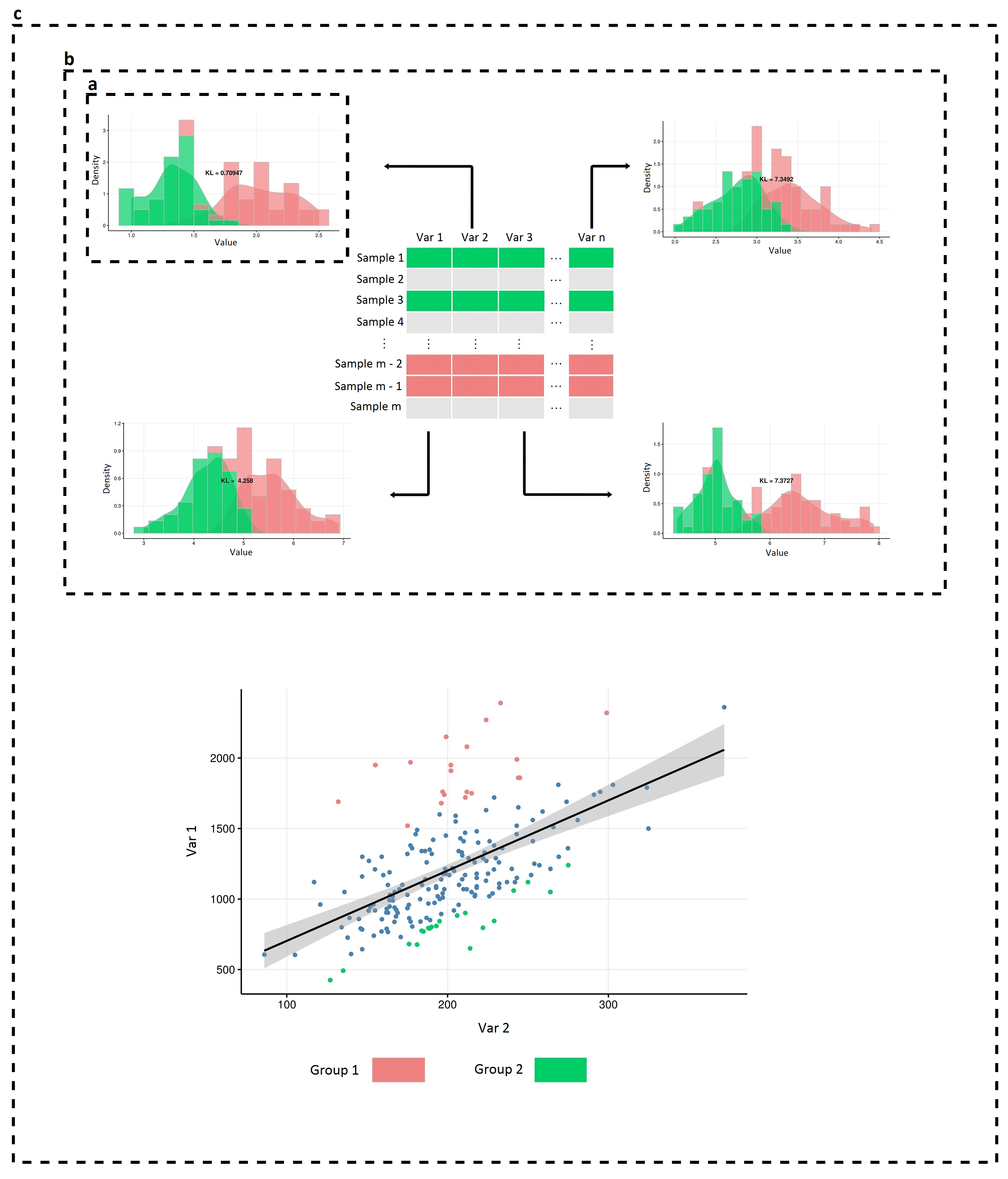
  Figure 1: Variable-wise KL-based methods. Given a multivariate dataset with $m$ samples and $n$ variables, a) simple (symmetric) KL-divergence (KL) can be used in order to find the distance between probability distributions of two interesting groups of sample, colored in green and red, for a single variable; b) Variable-wise KL-divergence (VKL) can be used so as to calculate KL-divergence between two groups of samples for each variable, by calculating KL-divergence between the two groups on each variable; c) by fitting a linear model on two variables of interest, Violating Variable-wise KL-divergence (VVKL), finds the outliers with most absolute residuals in the linear model, the upper group is colored in red and the lower one is in green and these two groups of outliers will be then passed to VKL to find the violating (blocking) variables for the linear association expected on the two variables.

  

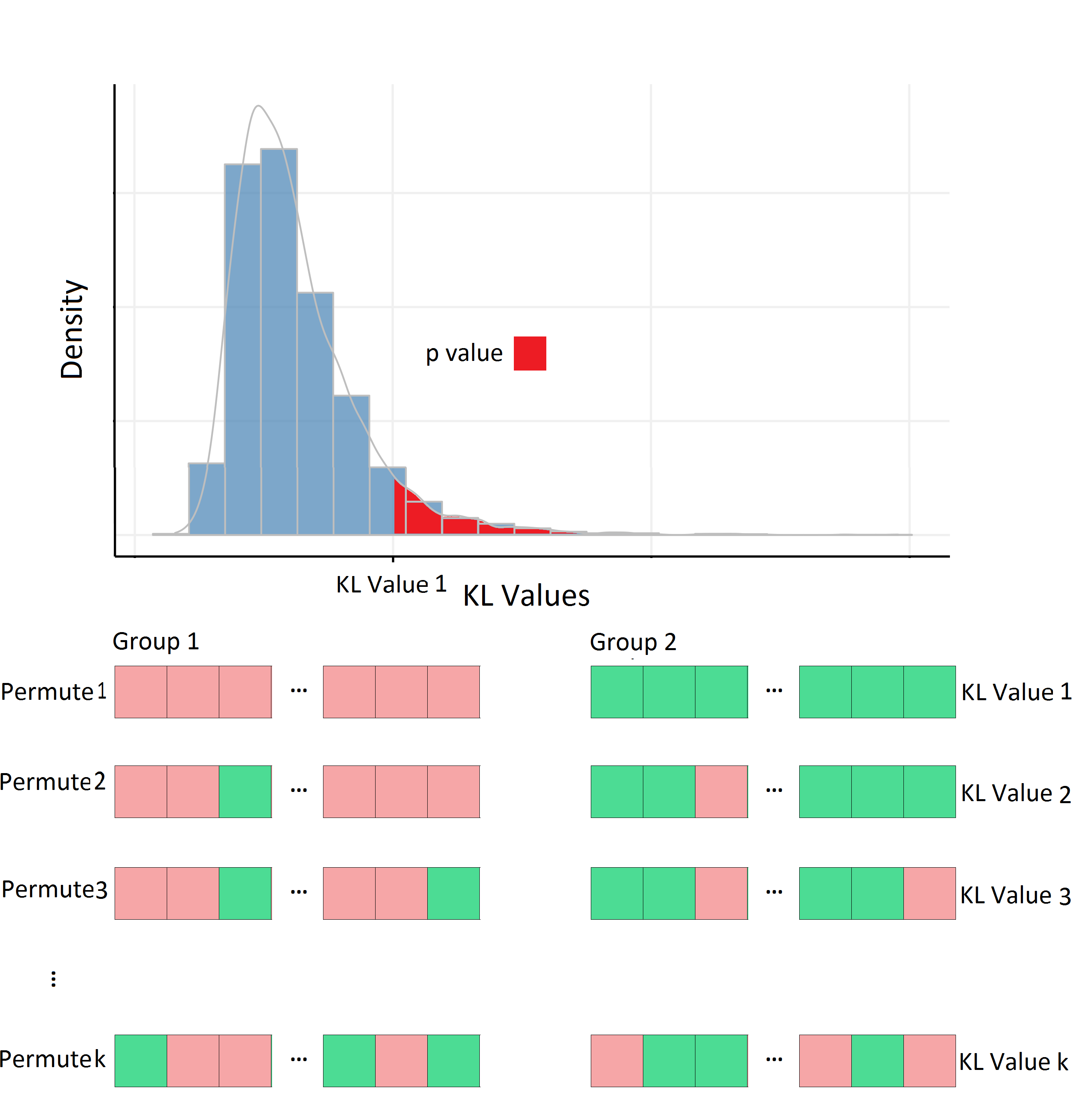
  Figure 2: The significance level of KL-divergence. In order to find the significance level of a KL-divergence (KL Value 1) of a variable between two groups of samples (Permute 1), one can permute the samples between groups for $k$ times and compute the KL-divergence between new couple of groups (Permute 2, Permute 3, $\dots$, Permute k). Afterward, one can find the significance level of the KL-value by considering the empirical distribution of permuted KL-values as it is illustrated in the upper plot.

3 Package Implementation

3.1 Preprocessing

The data_preproc function can be used to preprocess raw datasets. The function is designed to address outlier-detection and imputation of missing data. In order to find outliers, data_preproc uses an anomaly-detection algorithm from Vallis2014 for time series data (Fig. 3). For each variable, it sorts the observations in a decreasing (or increasing) order and it defines the anomalies detected by the algorithm, as outlier data (Fig. 4). The function then removes the outliers and behave them as missing observations. The missing observations are imputed by the mean or the median of the whole set of observations for the measurement if it is continuous or categorical, respectively. The method gets a parameter, levels, an integer value indicating the maximum number of levels of a categorical variable. The method returns the dataset with continuous variables as numeric and categorical variables as factor data types (see 4.2 for the practical example).

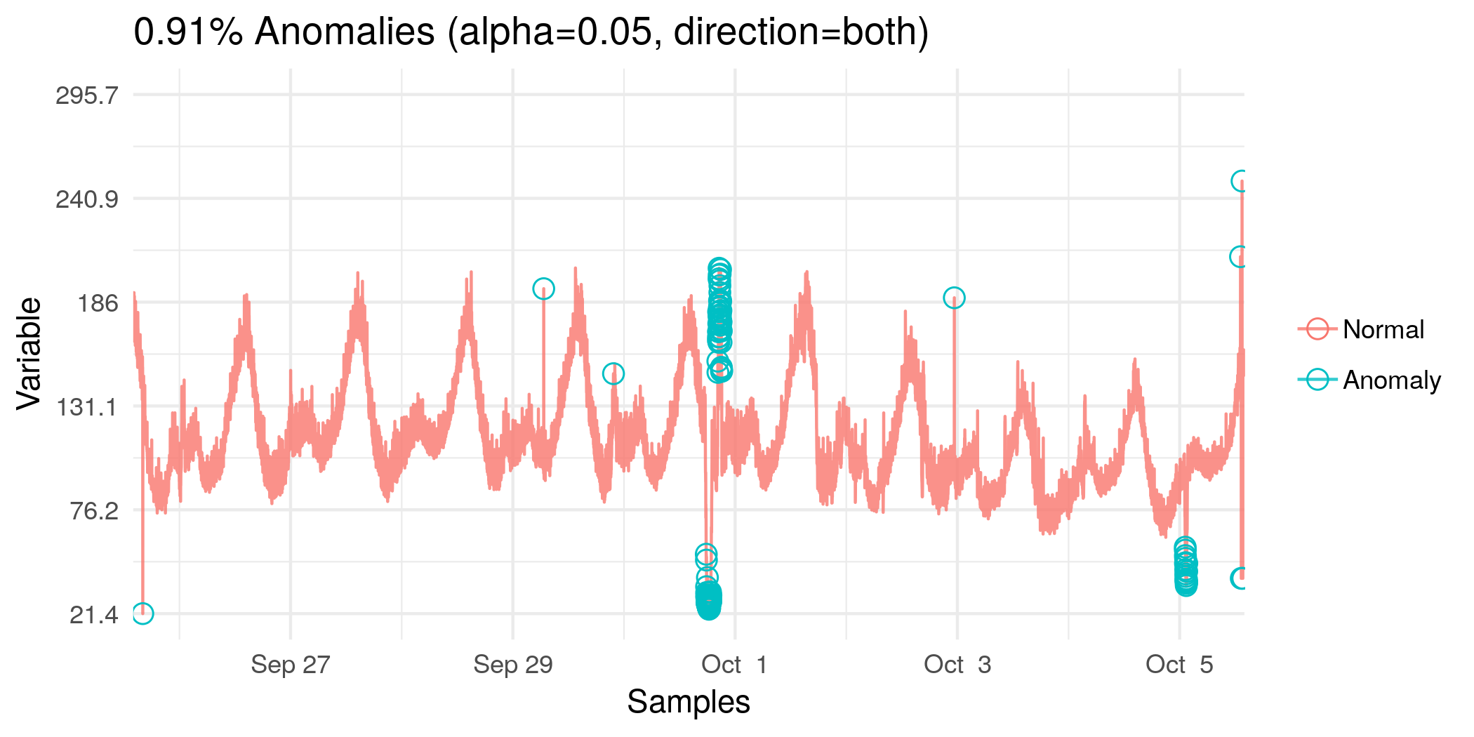
Figure 3: Anomaly Detection by Vallis2014. The points in time-series data which do not follow the major trend of data are recognized as anomalies. The normal samples are colored in red and the anomalies are in blue

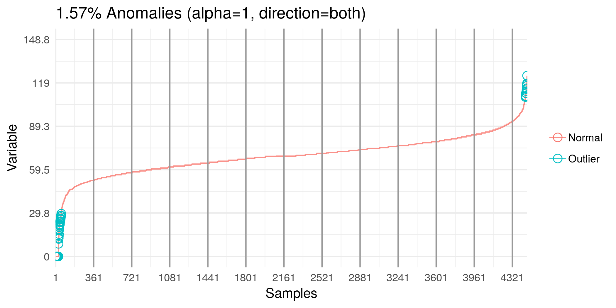
Figure 4: Outlier Detection Algorithm. After sorting data points in an increasing manner for the variable of interest, the outliers are detected after applying the anomaly detection algorithm (blue samples).

3.2 Test Associations

The function test_pair implements Pearson’s Chi-squared, ANOVA, and correlation tests for categorical-categorical, categorical-continuous, and continuous-continuous pairs of variables, respectively. One can easily use test_pair (test_assoc) in order to test any desired association between two (multiple) variables. Additionally, test_assoc implements multiple hypothesis tests, using False Discovery Rate correction of Benjamini and Hochberg.

3.3 Plot Associations

The function plot_assoc is implemented to facilitate single- and pairwise-variable visualizations. For a single continuous or categorical variable, it creates a bar plot and density plot, respectively. Pairwise-variable visualizations consist of a boxplot of the continuous variable for different levels of the categorical one, a scatter plot for two continuous variables and a heatmap illustrating the relation of different levels of two categorical variables. There is also a logical parameter interactive indicating if the output plot a highcharter object (highcharter). It will output a print-friendly plot using R package ggplot2 when the parameter is set to False (wickham2010ggplot2).

3.4 GMs

As mentioned in 2.1, GMs are efficient for computation and interpretation of the whole structure of associations among the variables. However, each set of variables requires a proper GM. Package muvis implements three types of GMs: (i) ggm implements five different methods (i.e., AIC-based, BIC-based, partial correlation thresholding, significance testing, and glasso) for GGM structure learning, based on R packages gRim, glasso, SIN, and gRbase. (ii) dgm is for constructing Directed (causal) GMs (DGMs) using pcalg package. (iii) min_forest is designed for High-dimensional Graphical Modeling and is based on its implementation in the package gRapHD (Rosa2010). For all of the mentioned methods, there is a parameter community which indicates if the user wants to apply community detection algorithms on the graph to find the modules within the graph. To this end, we used Louvain method from R package igraph (Csardi2010; Blondel2008). There is another parameter plot which is a logical parameter indicating if the user wants to plot the graph. The R package qgraph is used to implement this graph visualization (Epskamp2012).

3.5 KL-based Functions

The functions VKL and VVKL implement the KL-methods. The parameter permute indicates the number of permutations as described in • ‣ 2.2 and is used to find the significance of the KL values. We used the function KL.plugin from R package entropy to calculate KL values (Hausser2014). As this function works on discrete data, prior to calculating KL for continuous variables, we discretize and consider them like discrete data (see LABEL:vkl).

4 The NHANES 2005-2006 dataset

The National Health and Nutrition Examination Surveys (NHANES) (nhanes) is a program of studies about health and nutrition for US residents. We examined the functionality of muvis on NHANES 2005-2006 dataset which contains 7449 variables and 10,348 samples (see https://www.icpsr.umich.edu/icpsrweb/ICPSR/studies/25504/summary for more details).
Based on the number of missing values, we selected 161 variables including one ID, 74 continuous, and 86 categorical variables (having two to fifteen levels) and 4461 individuals (samples) aged from 20 to 85 years, including about 1% missing values. See Table LABEL:vars for description of the variables that are mentioned in this article. Complete list of 161 variables is available in NHANES dataset of the package. The next parts describe the analysis of this dataset using muvis.

4.1 Loading the package and the data

muvis is available at https://github.com/bAIo-lab/muvis. Once the package is installed and loaded into the R environment, the NHANES dataset can be loaded as a dataframe by a call to data as in the following. > library(muvis) > data("NHANES")

4.2 Preprocessing the data

We use data_preproc function for preprocessing of NHANES. The detect.outliers option is used to exclude outliers for each variable. As a first step through interpretation, we plot the relation between LBXVIE (a variable in the dataset indicating the amount of vitamin E) and LBXTC (the amount of total cholesterol) with and without outliers. The difference has been shown in Fig. 5. > nhanes_with_outliers <- data_preproc(NHANES, levels = 15, alpha = 0.5) > nhanes <- data_preproc(NHANES, levels = 15, detect.outliers = TRUE, alpha = 0.5) > plot_assoc(nhanes_with_outliers, vars = c("LBXVIE", "LBXTC")) > plot_assoc(nhanes, vars = c("LBXVIE", "LBXTC"))

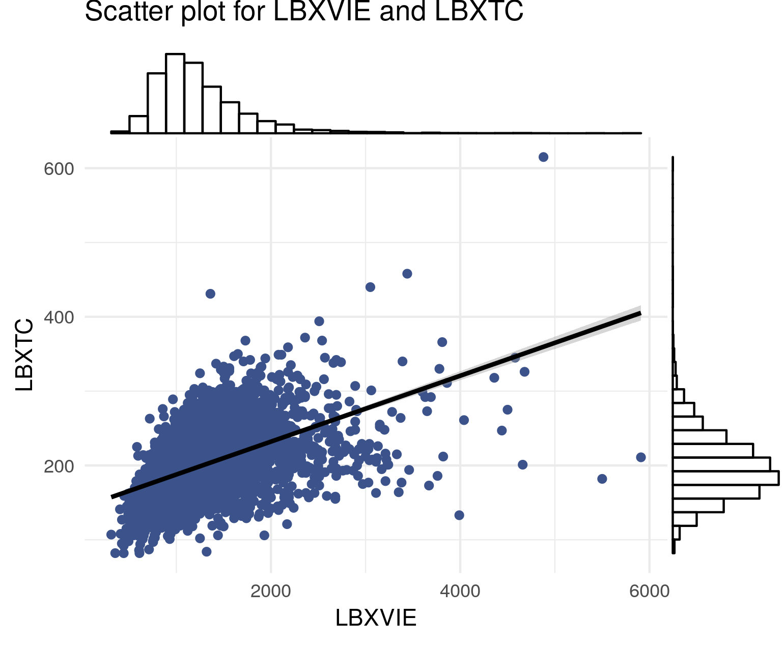
(a)

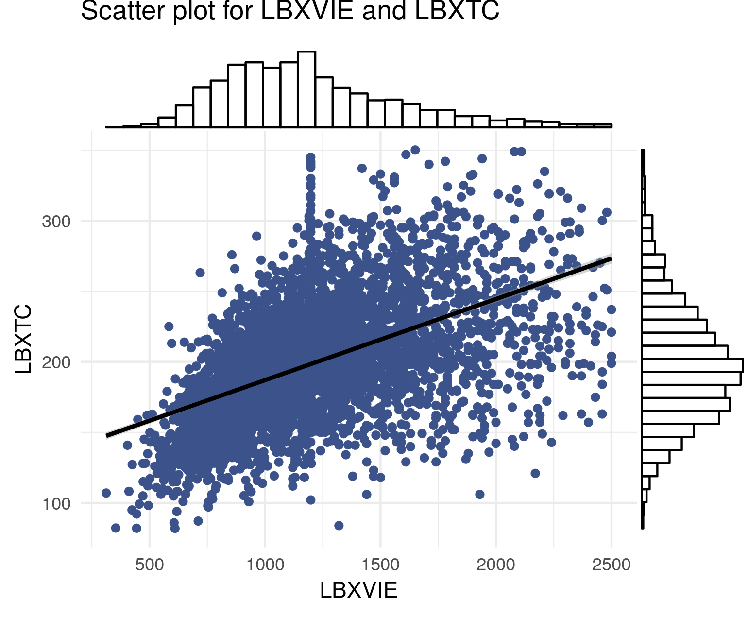
(b)

Figure 5: Scatter plot of LBXTC (total cholesterol. mg/dL) and LBXVIE (vitamin E. ug/dL) for NHANES dataset (a) with outliers and (b) without outliers. Each blue point indicates a sample and the black line shows the regression line fitted on two variables.

4.3 GGM for continuous data

We construct a GGM for continuous variables using ggm function. In this example, we construct it by intersecting glasso and sin algorithms. The largest connected component of the estimated graph is visualized by graph_vis function (Fig. 6). > nhanes$SEQN<-NULL>nhanes_{g}gm<-ggm(nhanes,significance=0.05,rho=0.15,community=TRUE,methods=c("glasso","sin"),plot=F)>grph_{c}lustrs<-clusters(nhanes_{g}gm$graph) > new_ggm <- induced.subgraph(nhanes_ggm$graph,V(nhanes_{g}gm$graph)[which(grph_clustrs$membership==which.max(grph_{c}lustrs$csize))]) > ggm_vis <- graph_vis(new_ggm, plot = T, filetype = "png", filename = "nhanes_ggm")

Investigating each community one can appraise the efficiency of the model: Community 1 are all about body measurements (e.g., BMI, waist circumstance, height, etc.); community 2 explains red blood cell profile; community 3 contains measurements about different types of white blood cells; community 4 accommodates uric acid, vitamin A, Urea, Creatinine, and Homocysteine; community 5 includes variables describing body biochemistry profile; community 6 contains some vitamins and chemical compounds (e.g. carotenoids, folate, etc.); and finally community 7 contains age, blood pressure, lead, and Parathyroid hormone.

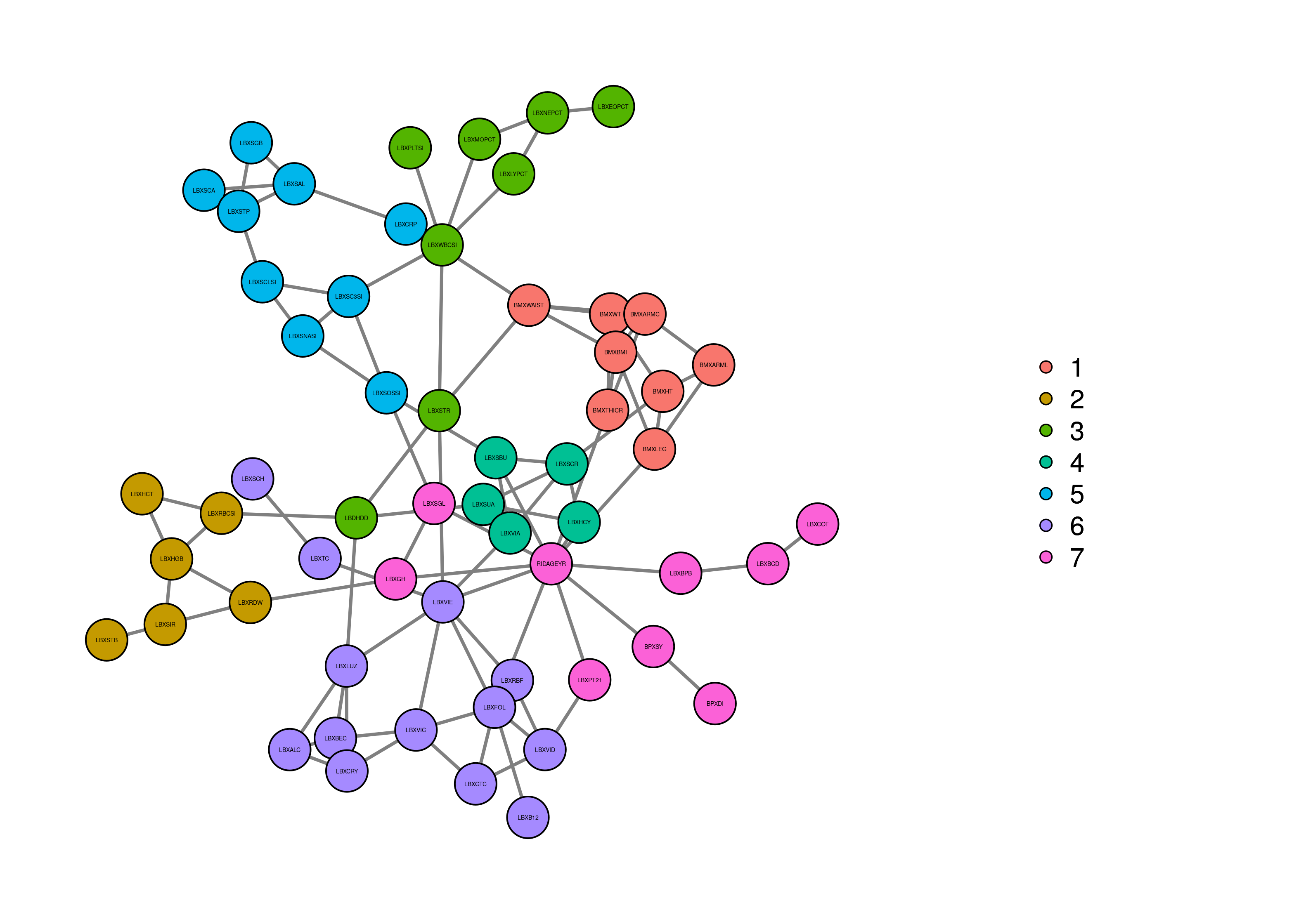
Figure 6: GGM. The graph is constructed using ggm function with the intersection of the models estimated by sin and glasso methods. The largest connected component of the graph is shown. The nodes represent continuous variables in the data and are colored according to their community.

4.4 Causal network for continuous data

The causal (directed) network of continuous variables is constructed using dgm function with parameter dtype = "gaussian". The largest connected component of the estimated graph is shown in Fig. LABEL:fig:dgm. > nhanes_dgm <- dgm(nhanes, dtype = "gaussian", alpha = 1e-15) > grph_clustrs <- clusters(nhanes_dgm$graph)>new_{d}gm<-induced.subgraph(nhanes_{d}gm$graph, V(nhanes_dgm$graph)[which(grph_{c}lustrs$membership == which.max(grph_clustrs$csize))])>dgm{}_{v}is<-graph{}_{v}is(new{}_{d}gm,plot=T,directed=T,filename=\mathrm{"}nhanes{}_{d}gm\mathrm{"},filetype=\mathrm{"}png\mathrm{"})\text{Figure 7Figure 77Figure 77Causal graph.Thelargest}$