Nonclassical states of levitated macroscopic objects beyond the ground state

Abstract

The preparation of nonclassical states of mechanical motion conclusively proves that control over such motion has reached the quantum level. We investigate ways to achieve nonclassical states of macroscopic mechanical oscillators, particularly levitated nanoparticles. We analyze the possibility of the conditional squeezing of the levitated particle induced by the homodyne detection of light in a pulsed optomechanical setup within the resolved sideband regime. We focus on the regimes that are experimentally relevant for the levitated systems where the ground-state cooling is not achievable and the optomechanical coupling is comparable with the cavity linewidth. The analysis is thereby performed beyond the adiabatic regime routinely used for the bulk optomechanical pulsed systems. The results show that the quantum state of a levitated particle could be squeezed below the ground state variance within a wide range of temperatures. This opens a path to test for the first time nonclassical control of levitating nanoparticles beyond the ground state.

I Introduction

Optomechanics Meystre (2013); *aspelmeyer_cavity_2014; *khalili_quantum_2016 is a field studying systems in which a light or microwave mode is coupled to mechanical motion via radiation pressure. It has developed at dramatic rates recently, particularly in providing access to strong coupling Gröblacher et al. (2009); *verhagen_quantum-coherent_2012, optomechanically induced transparency Weis et al. (2010), ground state cooling Chan et al. (2011); *teufel_sideband_2011, mechanical squeezing Wollman et al. (2015); Pirkkalainen et al. (2015), nonclassical correlations between photons and phonons Riedinger et al. (2016); *hong_hanbury_2017, and optomechanical entanglement Palomaki et al. (2013); Riedinger et al. (2018); Ockeloen-Korppi et al. (2018), all of which have been demonstrated in the lab. The remaining step would be to prove that control of the mechanics reaches a level incompatible with any mixture of classical motional states. To prepare and verify nonclassical aspects, a pulsed scheme Hofer et al. (2011); Vanner et al. (2011) would be advantageous. It unambiguously separates state preparation and verification Palomaki et al. (2013) and keeps the optomechanical system out of the unstable regime inherently peculiar to the optomechanical systems with a single continuous-wave pump Braginsky and Minakova (1964); *braginsky_ponderomotive_1967.

There is great interest in achieving nonclassical states of mechanics for enhancing metrological performance including force Rugar et al. (2004); Gavartin et al. (2012), mass Seveso et al. (2017) and displacement sensing Abbott et al. (2009); *ligo_scientific_collaboration_and_virgo_collaboration_observation_2016, magnetometry Forstner et al. (2012); *yu_optomechanical_2016; *li_quantum_2018, and biological applications Arndt et al. (2009). Optomechanical systems find application in the field of quantum information, particularly to transduce Bagci et al. (2014); *andrews_bidirectional_2014; *andrews_quantum-enabled_2015; *lecocq_mechanically_2016 and route Peterson et al. (2017); *barzanjeh_mechanical_2017; *malz_quantum-limited_2018; *ruesink_optical_2018 quantum signals. Moreover, a macroscopic object is of great use for testing the fundamental validity of quantum mechanics at larger mass scales Kaltenbaek et al. (2016); Lei et al. (2016); Santos et al. (2017) and probing decoherence models Romero-Isart (2011); *bera_proposal_2015; *vinante_improved_2017.

An excellent candidate for many applications happens to be optomechanics with levitated nanoparticles Chang et al. (2010); *romero-isart_optically_2011; Barker (2010); Kiesel et al. (2013); Yin et al. (2013). Levitated particles show great isolation from the environment and therefore, owing to the elimination of the clamping losses, exceptionally high mechanical Q-factors. The oscillatory motion of the nanoparticle is provided by the optical trap, and can therefore be engineered with great precision. Moreover, the optical potential for the nanoparticle can be adjusted to be nonlinear Dholakia and Čižmár (2011); Gieseler et al. (2013); Fonseca et al. (2016); Ricci et al. (2017); Šiler et al. (2017, 2018) and variable in time Konopik et al. (2018). Simultaneously, it can be controlled in the sideband resolved regime Kiesel et al. (2013); Millen et al. (2015) with full control of the linearized interaction between light and nanoparticle motion. At the same time, cooling the nanoparticles to the ground state is still challenging Gieseler et al. (2012); Asenbaum et al. (2013); Millen et al. (2015); Jain et al. (2016). Until now, only classical squashing has been demonstrated with levitating nanospheres Rashid et al. (2016).

In this paper we investigate the possibility for the linearized optomechanical interaction to create quantum correlations between a levitated particle and a control field. We show that these correlations are sufficient to steer the levitated particle into a conditionally squeezed state upon detection of the optical mode. To reach this, we use an amplifier interaction in the resolved sideband regime (at the blue sideband), however, we have to go beyond the adiabatic elimination of the intracavity field as the optomechanical coupling in the levitated systems in non-negligible with respect to the cavity decay. Therefore, we have to optimize the temporal modes of light beyond the frequently used exponential time profiles Hofer et al. (2011); Palomaki et al. (2013); Andrews et al. (2015). After this optimization, the measurement-induced preparation of mechanical squeezed states is tolerant to the occupations of the mechanical environment reaching $\sim 10^{7}$ phonons, what corresponds to the average occupation of a $100$ kHz oscillator at $50$ K.

II Pulsed Sideband-resolved Optomechanics

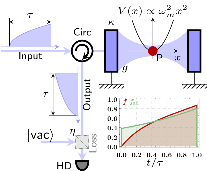
Figure 1: A sketch of the measurement-induced mechanical squeezing of levitated nanoparticle. The nanoparticle P is trapped in a harmonic potential by an auxiliary trapping beam (not shown). The motion of the particle is coupled to a mode of the cavity at rate $g$. The cavity is illuminated by a pulse (Input). In the presence of a strong blue-detuned pump the motion of the particle becomes correlated with a particular temporal mode of the leaking field (Output) directed via the circulator (Circ) to the homodyne detector (HD). Homodyne detection can project the mechanical system onto a displaced thermal squeezed state. Inset: example of the different mode shapes. Red (darker) line corresponds to the optimal mode defined by (15), green (lighter) to the approximate exponential modes (20).

In this section, following the usual textbook approach Bowen and Milburn (2015), we derive the equations of motion for the effective two-mode squeezing interaction in an optomechanical system.

We consider a standard optomechanical system Aspelmeyer et al. (2014) which has an optical mode coupled to the centre of mass motion of a levitated particle via radiation pressure (see Fig. 1). The mechanical motion modulates the cavity frequency, which gives rise to the standard optomechanical Hamiltonian (we use $\hbar=1$) Law (1995); Chang et al. (2010); *romero-isart_optically_2011; Monteiro et al. (2013)

$$H=[\omega_{\text{cav}}-g_{0}(a_{m}^{\dagger}+a_{m})]a_{c}^{\dagger}a_{c}+\omega_{m}a_{m}^{\dagger}a_{m}+H_{\text{pump}},$$ (1)

where $a_{c}(a_{m})$ is the annihilation operator of the cavity (mechanical) mode with the eigenfrequency $\omega_{\text{cav}}(\omega_{m})$, and $g_{0}$ is the single-photon optomechanical coupling rate approximately showing the cavity frequency modulation per mechanical quanta. We assume the system to be in the presence of a strong coherent pump at frequency $\omega_{p}=\omega_{c}-\Delta$ which is used to enhance the weak optomechanical interaction

$$H_{\text{pump}}=i\mathcal{E}(a_{c}^{\dagger}e^{-i\omega_{p}t}-a_{c}e^{i\omega_{p}t}).$$ (2)

The strong coherent pump creates a mean classical displacement of both the cavity mode and the mechanical mode, so that each mode experiences weak quantum fluctuations around those mean displacements. We proceed by linearizing the dynamics around the classical displacements and consider the quantum evolution of the fluctuating parts. Thereby in a rotating frame given by $H_{\text{rf}}=\omega_{p}a_{c}^{\dagger}a_{c}+\omega_{m}a_{m}^{\dagger}a_{m}$ the linearized Hamiltonian takes the form (to simplify the equations we keep notation $a_{i}$ for only the fluctuating parts)

$$H=\Delta a_{c}^{\dagger}a_{c}-g(a_{c}^{\dagger}+a_{c})(a_{m}^{\dagger}e^{i\omega_{m}t}+a_{m}e^{-i\omega_{m}t}),$$ (3)

where $g=g_{0}\sqrt{\left\langle N_{\text{ph}}\right\rangle}$ is the coupling rate enhanced by the mean number of intracavity photons $\left\langle N_{\text{ph}}\right\rangle$. This is the standard Hamiltonian of the linearized optomechanical interaction. It has been successfully demonstrated in experiments to correctly describe the dynamics of the optomechanical systems in different regimes set by the detuning $\Delta$, e.g., in Gröblacher et al. (2009); Verhagen et al. (2012); Chan et al. (2011); *teufel_sideband_2011; Palomaki et al. (2013); Millen et al. (2015).

In this manuscript we investigate the dynamics of an optomechanical system tuned to the blue sideband ($\Delta=-\omega_{m}$). To derive the effective Hamiltonian for this regime, we first go to the rotating frame defined by $H_{\text{rf}}^{\prime}=\Delta a_{c}^{\dagger}a_{c}$, and then apply the rotating wave approximation to cancel the terms rapidly counter-rotating at $2\omega_{m}$. The latter requires the mechanical frequency $\omega_{m}$ be the dominant rate in the system, which practically is equivalent to the condition of the cavity decay $\kappa$ being much smaller than the mechanical frequency ($\kappa\ll\omega_{m}$, so-called resolved sideband condition). Then,

$$H=-g(a_{c}^{\dagger}a_{m}^{\dagger}+a_{c}a_{m}).$$ (4)

This interaction is known to entangle the parties even in presence of large amounts of noise Filip and Kupčík (2013); Rakhubovsky and Filip (2015), so it is a natural choice to use this interaction for creating an entangled state of light and mechanics. Unfortunately there is an inherent instability associated with this type of interaction in optomechanical systems Braginsky and Minakova (1964); *braginsky_ponderomotive_1967. Tuned on the right slope of the cavity resonance curve (blue sideband), the coherent pump creates an effective spring for the mechanical mode. Simultaneously, a negative damping (amplification) is created. This negative damping might overwhelm the inherently low intrinsic damping of a high-Q mechanical system, thus rendering it unstable and making the steady state of the system inaccessible. A natural way to compensate for this is to avoid steady states, and to shift attention to pulses Vanner et al. (2011); Hofer et al. (2011); Vanner et al. (2013).

Using the Hamiltonian (4), we can write the quantum Langevin equations introducing the damping and noise terms. Since the Hamiltonian of the linearized optomechanical interaction is at most quadratic in the bosonic operators, the equations of motion are linear. These equations can be written in the matrix form Genes et al. (2009)

$$\dot{\bm{u}}=\mathbb{A}\bm{u}+\sqrt{2\mathbb{K}}\bm{n},$$ (5)

where $\bm{u}=(X_{c},Y_{c},X_{m},Y_{m})^{\text{T}}$ is the vector of unknowns and $\bm{n}=(X^{\text{in}},Y^{\text{in}},X^{\text{th}},Y^{\text{th}})^{\text{T}}$ is the vector of the quadratures of the input quantum noises, the superscript ${}^{\text{T}}$ denotes transposition. The quadratures $X^{\text{in}}$ and $Y^{\text{in}}$ describe the input vacuum field of optical fluctuations, and $X^{\text{th}}$ and $Y^{\text{th}}$ are the quadratures of the thermal Langevin force acting upon the mechanical mode. We use the convention $X_{j}=a_{j}+a_{j}^{\dagger},Y_{j}=(a_{j}-a_{j}^{\dagger})/i$ for $j=c,m$, so that $\left[X_{j},Y_{j}\right]=2i$. The operators of the environment obey $\left[X^{k}(t),Y^{k}(t^{\prime})\right]=2i\delta(t-t^{\prime})$, for $k=\text{in, th}$. Also we assume they obey the standard Markovian autocorrelations Giovannetti and Vitali (2001), e.g., $\left\langle X^{\text{in}}(t)X^{\text{in}}(t^{\prime})\right\rangle=\delta(t-t^{\prime})$ and $\left\langle X^{\text{th}}(t)X^{\text{th}}(t^{\prime})\right\rangle=(2n_{\text{th}}+1)\delta(t-t^{\prime})$ with $n_{\text{th}}$ being the average occupation of the bath. Furthermore, $\mathbb{K}=\operatorname*{\operatorname{diag}}(\kappa,\kappa,\gamma/2,\gamma/2)$ is the diagonal matrix composed of optical damping rate $\kappa$ and the mechanical viscous damping rate $\gamma$, and $\mathbb{A}$ is the so-called drift matrix. For the case of the two-mode squeezing interaction, the drift matrix has the form

$$\mathbb{A}=\begin{pmatrix}-\kappa&0&g&0\\ 0&-\kappa&0&-g\\ g&0&-\gamma/2&0\\ 0&-g&0&-\gamma/2\\ \end{pmatrix}$$ (6)

Here and throughout the article we assume $\left\langle N_{\text{ph}}\right\rangle$ (and thereby $g$) independent of time. This is a valid approximation for a top-hat drive with constant pump strength equal $\mathcal{E}(t)=\mathcal{E}$ within the pulse duration $0\leq t\leq\tau$ and zero otherwise. Another requirement is that the pulse duration is longer than the cavity decay time $\kappa\tau\gg 1$, for example as in Palomaki et al. (2013).

Eq. 5 has the formal solution

$$\bm{u}(t)=\mathbb{M}(t)\bm{u}(0)+\int_{0}^{t}\mathrm{d}s\>\mathbb{M}(t-s)\sqrt{2\mathbb{K}}\bm{n}(s),$$ (7)

where

$$\mathbb{M}(s)=\exp[\mathbb{A}s].$$ (8)

Importantly, for a bipartite system, an analytical form of $\mathbb{M}$ can always be computed however in general it is too cumbersome to be reported here. In the general case of a time-dependent pump strength, Eq. 5 should be solved numerically.

III Optimized temporal modes of light

The solution (7) is sufficient to analyze the optomechanical dynamics, particularly the transfer of quantum information from the incident light to the mechanical mode. Among other terms, the expression for the mechanical mode contains a term corresponding to the input optical quantum fluctuations serving as the signal

$$X_{m}(\tau)=\dots+\int_{0}^{\tau}\mathrm{d}s\>\mathbb{M}_{31}(\tau-s)\sqrt{2\kappa}X^{\text{in}}(s)\\ =\dots+\sqrt{\mathfrak{G}-1}\mathcal{X}^{\text{in}},$$ (9)

where we have designated the quadratures of the input optical temporal mode and the optomechanical amplification gain $\mathfrak{G}$ as

$$(\mathcal{X}^{\text{in}},\mathcal{Y}^{\text{in}})^{\text{T}}\equiv\int_{0}^{\tau}\mathrm{d}s\>f^{\text{in}}(s)(X^{\text{in}}(s),Y^{\text{in}}(s))^{\text{T}},$$ (10)

$$f^{\text{in}}(s)=\sqrt{\frac{2\kappa}{\mathfrak{G}-1}}\mathbb{M}_{31}(\tau-s),$$ (11)

$$\mathfrak{G}=1+2\kappa\int_{0}^{\tau}\mathrm{d}s\>\mathbb{M}_{31}^{2}(s).$$ (12)

The definition of $\mathcal{Y}^{\text{in}}$ features the same $f^{\text{in}}$ as the one for $\mathcal{X}^{\text{in}}$ owing to the symmetries in $\mathbb{A}$ that secure $\mathbb{M}_{31}(s)=-\mathbb{M}_{42}(s)$. This way we select a single temporal mode— the optimally coupled one— from the continuum of the temporal modes of the input fluctuations. By definition, this mode has proper commutation relations $\left[\mathcal{X}^{\text{in}},\mathcal{Y}^{\text{in}}\right]=2i$, because $\int_{0}^{\tau}\mathrm{d}s\>(f^{\text{in}}(s))^{2}=1.$

To complete the consideration of the system, we have to supplement the equations above with an input-output relation in the form

$$\bm{v}^{\text{out}}(t)=-\tilde{\bm{n}}^{\text{in}}(t)+\sqrt{2\kappa}\tilde{\bm{u}}(t),$$ (13)

where $\bm{v}^{\text{out}}=(X^{\text{out}},Y^{\text{out}})^{\text{T}}$, and the tilde denotes that we take the only first two entries of the vector, e.g. $\tilde{\bm{u}}=(\bm{u}_{1},\bm{u}_{2})^{\text{T}}$.

In a similar fashion with the solution for the intracavity quadratures, we conclude that the expression for the leaking field has a term

$$X^{\text{out}}(t)=\dots+\mathbb{M}_{13}(t)\sqrt{2\kappa}X_{m}(0).$$ (14)

Therefore, the proper temporal mode of the leaking field, which is optimally coupled to the mechanical mode, is defined by the profile of the interaction $\mathbb{M}_{13}(t)$. We thus define the quadratures of the output mode in full analogy with the definition for the input mode:

$$(\mathcal{X}^{\text{out}},\mathcal{Y}^{\text{out}})^{\text{T}} \equiv\int_{0}^{\tau}\mathrm{d}s\>f^{\text{out}}(s)(X^{\text{out}}(s),Y^{\text{out}}(s))^{\text{T}},$$ (15)

$$f^{\text{out}}(s) =\sqrt{\frac{2\kappa}{\mathfrak{G}-1}}\mathbb{M}_{13}(s),$$ (16)

Again, owing to the symmetries in $\mathbb{A}$, $\mathbb{M}^{\text{T}}=\mathbb{M}$ and therefore

$$\int_{0}^{\tau}\mathrm{d}s\>\mathbb{M}_{13}^{2}(s)=\int_{0}^{\tau}\mathrm{d}s\>\mathbb{M}_{31}^{2}(s)=\frac{\mathfrak{G}-1}{2\kappa}.$$ (17)

Defined by (15), the output mode obeys proper commutations $\left[\mathcal{X}^{\text{out}},\mathcal{Y}^{\text{out}}\right]=2i$, and carries maximum information regarding the initial mechanical state. Note that if, instead, a different temporal mode is measured it will carry only a certain fraction of the information, with this fraction defined by the temporal overlap of the profiles of the modes.

In the general case, the elements of $\mathbb{M}$ and, therefore, the temporal shapes of the optimal modes of the radiation, have a complicated dependence on time. In certain important cases, however, there exist simple approximations to the exact temporal shapes. Particularly, for the case of a two-mode squeezing optomechanical interaction with Hamiltonian (4), the corresponding functions take the form

$$f^{\text{out}}(s)\propto\mathbb{M}_{13}(t)=\frac{g}{\lambda}\left[e^{-\tfrac{t}{2}(\kappa+\frac{\gamma}{2}-\lambda)}-e^{-\tfrac{t}{2}(\kappa+\frac{\gamma}{2}+\lambda)}\right],$$ (18)

with $\lambda=\sqrt{(\kappa-\gamma/2)^{2}+4g^{2}}$. In the case of wide-band cavity $\kappa\gg g,\gamma$ the intracavity mode can almost instantaneously react to the other influences, and therefore can be adiabatically eliminated. Thereby, in this adiabatic regime the expression for the leaking mode shape can be simplified and transforms into

$$f^{\text{out}}_{\text{ad}}(t)\propto e^{Gt},$$ (19)

where we define the optomechanical amplification rate $G=g^{2}/\kappa$. In a similar fashion one can process the temporal shape of the incident pulse to obtain the expressions of the input and output modes’ temporal shape functions as follows

$$f_{\text{ad}}^{\text{in}}(t)=\sqrt{\frac{2G}{1-e^{-2G\tau}}}e^{-Gt},\quad f_{\text{ad}}^{\text{out}}(t)=\sqrt{\frac{2G}{e^{2G\tau}-1}}e^{Gt},$$ (20)

The input-output transformations for the optical and the mechanical mode then read (for rather long pulses $\kappa\tau\gg 1$ and ignoring the mechanical decoherence for now)

$$\mathcal{A}^{\text{out}} =\sqrt{\mathfrak{G}}\mathcal{A}^{\text{in}}+\sqrt{\mathfrak{G}-1}a_{m}^{\dagger}(0),$$ (21a)

$$a_{m}(\tau) =\sqrt{\mathfrak{G}}a_{m}(0)+\sqrt{\mathfrak{G}-1}\mathcal{A}^{\text{in,}}{}^{\dagger}.$$ (21b)

The Bogoliubov transformations above correspond to the two-mode squeezing of the optical and the mechanical modes with the amplification coefficient $\mathfrak{G}=e^{2G\tau}$. For the sake of compactness of notation we have introduced the bosonic operators $\mathcal{A}^{k}=\frac{1}{2}(\mathcal{X}^{k}+i\mathcal{Y}^{k}),$ for $k=\text{in, out}$.

IV Conditional squeezing in the adiabatic regime

The two-mode squeezing interaction is known for its ability to entangle the modes and produce correlations sufficient to achieve conditional squeezing (CS) Filip and Kupčík (2013); Rakhubovsky and Filip (2015). The latter effect manifests itself as a projection of one of the two correlated modes onto a state which has the variance of one of the quadratures below the shot-noise level. In this section we introduce the formal definition of this effect and reiterate the sufficient conditions for the observation of CS in an experiment.

The state of the optomechanical system after the interaction is characterized by the vector $\bm{r}=(\mathcal{X}^{\text{out}},\mathcal{Y}^{\text{out}},X_{m}(\tau),Y_{m}(\tau))^{\text{T}}$. Since the system undergoes linear dynamics described by (5) with the initial state being Gaussian, the final state of the system remains Gaussian and can therefore be completely described by a vector of means $\left\langle\bm{r}\right\rangle$ and the covariance matrix (CM) $\mathbb{V}$. The latter is defined as a matrix with elements

$$\mathbb{V}_{ij}=\left\langle\bm{r}\circ\bm{r}\right\rangle_{ij}\equiv\tfrac{1}{2}\left\langle\left\{(\bm{r}_{i}-\left\langle\bm{r}\right\rangle_{i}),(\bm{r}_{j}-\left\langle\bm{r}\right\rangle_{j})\right\}\right\rangle,$$ (22)

where $\left\{a,b\right\}\equiv ab+ba$ is the anticommutator, and the averaging is performed in the quantum mechanical sense $\left\langle a\right\rangle\equiv\operatorname*{\operatorname{Tr}}(\rho a).$

Regrouping for convenience the elements of the vector $\bm{r}$ into $\bm{r}^{\text{out}}=(\mathcal{X}^{\text{out}},\mathcal{Y}^{\text{out}})^{\text{T}}$ and $\bm{r}_{m}=(X_{m},Y_{m})^{\text{T}}$, we can write the CM in the block form

$$\mathbb{V}=\begin{pmatrix}\mathbb{V}^{\text{out}}&\mathbb{V}^{c}\\ \mathbb{V}^{c,}{}^{\text{T}}&\mathbb{V}^{m}\end{pmatrix}$$ (23)

with

$$\mathbb{V}^{\text{out}}=\left\langle\bm{r}^{\text{out}}\circ\bm{r}^{\text{out}}\right\rangle,\mathbb{V}^{m}=\left\langle\bm{r}_{m}\circ\bm{r}_{m}\right\rangle,\mathbb{V}^{c}=\left\langle\bm{r}^{\text{out}}\circ\bm{r}_{m}\right\rangle.$$

The blocks on the main diagonal show the autocorrelations of the leaking pulse and the mechanical mode respectively, and the off-diagonal block show the cross-correlations between the two.

Upon homodyne detection of an amplitude quadrature ($\mathcal{X}^{\text{out}}$) of the leaking pulse, the mechanical mode is projected onto a Gaussian state with CM $\mathbb{V}^{m}{}^{\prime}$ given by Weedbrook et al. (2012)

$$\mathbb{V}^{m}{}^{\prime}=\mathbb{V}^{m}-\left[\mathbb{V}^{\text{out}}_{11}\right]^{-1}\mathbb{V}^{c}{}^{\text{,T}}\mathbb{P}\mathbb{V}^{c},$$ (24)

with $\mathbb{P}=\operatorname*{\operatorname{diag}}(1,0)$. For the generalization to the case of an arbitrary quadrature homodyne measurement see Appendix B. The state is squeezed if the smaller eigenvalue $\sigma_{\text{cond}}$ (for which we use the term conditional variance) of $\mathbb{V}^{m}{}^{\prime}$ is below the uncertainty of the vacuum $\sigma_{\text{vac}}$. For our choice of the commutation relations $\left[X_{m},Y_{m}\right]=2i$, $\sigma_{\text{vac}}=1$. In the simple case of a diagonal $\mathbb{V}^{m}{}^{\prime}$ the matrix elements on the principal diagonal have the meaning of uncertainties of the quadratures. The conditional variance is therefore equal to the smaller diagonal element and has the very illustrative meaning of the uncertainty of the squeezed quadrature.

In the case of the two-mode squeezing interaction, described by (21), the mechanical mode is projected by the homodyne detection of the amplitude quadrature of the leaking pulse on the state with the covariance matrix Filip and Kupčík (2013)

$$\mathbb{V}^{m}{}^{\prime}=\operatorname*{\operatorname{diag}}\left(\frac{2n_{0}+1}{\mathfrak{G}+(\mathfrak{G}-1)(2n_{0}+1)},2\mathfrak{G}(n_{0}+1)-1\right),$$ (25)

with $n_{0}$ being the initial occupation of the mechanical mode. In the experimentally relevant limit of high occupation, the covariance matrix simplifies to

$$\mathbb{V}^{m}{}^{\prime}\Big{|}_{n_{0}\gg 1}=\operatorname*{\operatorname{diag}}\left(\frac{1}{\mathfrak{G}-1},2\mathfrak{G}n_{0}\right),$$ (26)

which is squeezed regardless of the initial occupation provided $\mathfrak{G}>2$. Importantly, the squeezing occurs upon measurement of an arbitrary quadrature which is a manifestation of the phase insensitivity of the two-mode squeezing interaction. That is, regardless of which quadrature of light is measured, the eigenvalues of the covariance matrix $\mathbb{V}^{m}{}^{\prime}$ remain the same, although the eigenvectors might be rotated. Moreover, the final state of the mechanical mode is displaced in the phase space dependent on the outcome of the measurement of the optical mode. Such a displacement however does not affect the nonclassicality.

V Realistic conditional squeezing of a levitated nanoparticle

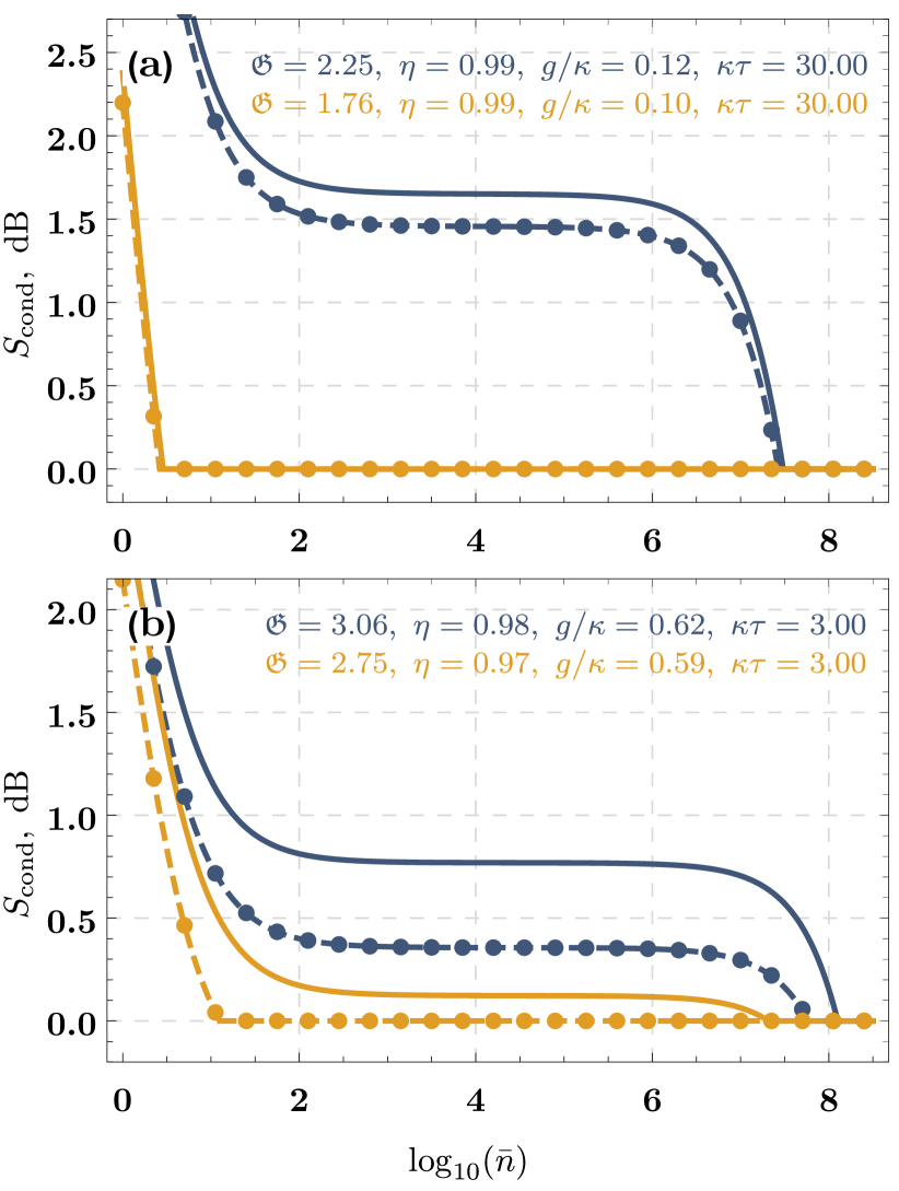
Figure 2: Conditional squeezing of a levitated particle as a function of temperature. We consider the mechanical mode to be in equilibrium with the environment before the pulsed protocol, so $n_{0}=n_{\text{th}}=\bar{n}$. Both panels make use of full solution of Eq. 5 without further approximations. (a) — close to the adiabatic regime, (b) — beyond the adiabatic regime. Different colors correspond to different choices of coupling strength $g$ and the pulse duration $\tau$, leading to different values of effective gain $\mathfrak{G}$ and loss $\eta$. The plateau in squeezing magnitudes, predicted by the adiabatic regime, remains in the full solution. Solid and dashed lines correspond to an ideal detection of, respectively, the optimal (15) and the exponential (20) mode of the leaking pulse. The lines with markers overlapping with the dashed lines correspond to the detection of the optimal mode that experienced a loss with transmittance equivalent to that provided by the overlap of the optimal and the exponential modes envelope (see (30)).

As can be seen from the previous section, under idealized conditions, the blue-detuned optomechanical interaction produces the thermal equivalent of a two-mode squeezed state of the leaking field and the levitated particle. In this section we evaluate the effect of imperfections in the system and analyze the potential to achieve conditional squeezing in state-of-the art experiments.

The idealized solution (21) analyzed in the previous section does not include mechanical decoherence, involves adiabatic elimination of the cavity mode and ignores optical losses. The first two effects are taken into account by considering the full solution of (5); the machinery for this evaluation is described in Appendix A. The optical loss enters at different stages of the protocol and in particular it manifests itself in nonunit photon escape and photodetection efficiencies, losses in the mirrors and in propagation etc. Advantageously, all these effects can be treated as a linear admixture of vacuum to the output signal (see Fig. 1). Thereby, the optical loss can be taken into account by modifying the input-output relation (13) as

$$\bm{v}^{\text{out}}(t)=\sqrt{\eta}\left[-\tilde{\bm{n}}^{\text{in}}(t)+\sqrt{2\kappa}\tilde{\bm{u}}(t)\right]\\ +\sqrt{1-\eta}\bm{v}^{\text{vac}}(t),$$ (27)

with $0\leq\eta\leq 1$ being the total transmittance associated with all the loss sources combined ($\eta=1$ corresponding to the lossless case), and $\bm{v}^{\text{vac}}=(\mathcal{X}^{\text{vac}},\mathcal{Y}^{\text{vac}})^{\text{T}}$ describing the joint vacuum mode of light. Following the modification described by (27), the covariance matrix $\mathbb{V}$ becomes

$$\mathbb{V}\to\begin{pmatrix}\eta\mathbb{V}^{\text{out}}&\sqrt{\eta}\mathbb{V}^{c}\\ \sqrt{\eta}\mathbb{V}^{c}{}^{\text{,T}}&\mathbb{V}^{m}\end{pmatrix}$$ (28)

Note that we do not have to consider the losses associated with the input light, since it is already in vacuum state, thereby an admixture of vacuum fluctuations to it does not modify the statistics of the input light.

The results of our simulations can be seen at Fig. 2. We plot the conditional squeezing in dB as a function of the initial occupation of the levitated nanoparticle which we assume to be in equilibrium with its environment (so that $n_{0}=n_{\text{th}}=\bar{n}$). The plotted quantity is therefore

$$S_{\text{cond}}=\max\left(0,-20\log_{10}\left[\sigma_{\text{cond}}(\bar{n})\right]\right).$$ (29)

Our analysis shows that in the regime of the parameters satisfying the requirements of the adiabatic interaction ($\kappa\gg g,\tau^{-1},\gamma$ and $\gamma n_{\text{th}}\tau\ll 1$) the full solution exhibits good correspondence with the approximate adiabatic one. As the occupation increases from the ground state, the magnitude of squeezing decreases until it reaches a plateau that spans over a few orders of magnitude of the occupation number values. The plateau is as well predicted by the adiabatic regime (cf. Eqs. 25 and 26). In accordance with this prediction, the magnitude of squeezing is determined solely by the amplification gain $\mathfrak{G}$ albeit the dependence is more complicated than in the adiabatic regime. Once the gain is above a certain threshold, the CS is possible for a wide range of temperatures, impossible for gain values below threshold (compare blue [darker] and yellow [lighter] lines in Fig. 2 (a)). The CS occurs regardless of which quadrature of the leaking field is measured, which is consistent with the phase insensitivity of two-mode squeezing.

The most important limiting factor in conditionally squeezing the mechanics is the nonzero initial occupation $n_{0}$ of the levitated particle and the occupation $n_{\text{th}}$ of its bath. In Fig. 2 we assume that the particle is initially at equilibrium with the surroundings, so $n_{0}=n_{\text{th}}$. The two occupations though have different effects on the possibility of the CS. For low values of the initial mechanical occupation $n_{0}$, before the plateau, the value of $n_{0}$ sets the upper boundary for the magnitude of the CS of the mechanical oscillator in accordance with (25). This occupation alone however does not impose limits on the CS, that is, in the case of zero occupation of the bath $n_{\text{th}}=0$, CS is possible for an arbitrary $n_{0}$ provided that the optomechanical amplification gain $\mathfrak{G}$ is above a certain threshold. Additionally the occupation of the bath $n_{\text{th}}$ does not influence the magnitude of the CS as long as it is below a certain value related to the rethermalization time $n_{\text{th}}\lesssim n^{\text{crit}}\equiv(\gamma\tau)^{-1}$. Above this value of $n_{\text{th}}$ the CS is impossible regardless of the initial occupation $n_{0}$. We would like to emphasize that this means that if for a given temperature of the bath the CS happens to be impossible, precooling alone does not salvage the situation.

Intuitively, in order to push the boundary of the temperatures allowing the CS up, one would shorten the pulse duration $\tau$ which means a shorter interaction with the bath and therefore a smaller amount of noise entering the mechanical mode. Indeed this helps however the appropriate values of $\tau$ are limited from below by the inverse cavity linewidth: $\tau\gtrsim\kappa^{-1}$, apparently because shorter pulses are unable to properly enter and leave the cavity. This, combined with the requirement of a resolved side-band, $\kappa\ll\omega_{m}$, sets a limit on the occupations of the bath, allowing the CS. The upper boundary for the phonon number is $n^{\text{crit}}\lesssim\omega_{m}/\gamma=Q_{m}$.

Decreasing the pulse duration $\tau$ causes a decrease of the amplification gain $\mathfrak{G}$ and thereby requires an increase in the optomechanical interaction rate $g$ in order to compensate it. The latter can be increased by increasing the intracavity power and subsequently the average number of the intracavity photons $\left\langle N_{\text{ph}}\right\rangle$. Decreasing $\tau$, and increasing $g$ such that it becomes comparable with $\kappa$ leads us farther from the adiabatic regime, which means that the optimal temporal mode of the leaking field increasingly differs from the simple exponential form (20). The analysis presented in Fig. 2 shows that the detection of an approximate exponential mode (20) (dashed lines) is indistinguishable from the detection of the optimal mode (15) preceded by an optical loss (lines with markers). The associated transmittance $\eta$ of the loss is exactly equivalent to the overlap of the temporal profiles of the modes:

$$\eta_{\text{mm}}=\int_{0}^{\tau}\mathrm{d}s\>f^{\text{out}}(s)f^{\text{out}}_{\text{ad}}(s),$$ (30)

where $f^{\text{out}}(s)\propto\mathbb{M}_{13}(s)$ is defined by the full solution of the equations of motion, and $f^{\text{out}}_{\text{ad}}(s)$, by the adiabatic solution (20). Both these functions are illustrated in the inset of Fig. 1. From the comparison of the magnitudes of CS attainable by the lossless and lossy detection it is evident that the optical loss can be a critical limiting factor to the extent that it renders the CS impossible at the temperatures at which a lossless detection would allow (see yellow [lighter] lines in Fig. 2 (b)). Note however that the deviation from the adiabatic regime, which invalidates the elimination of the cavity mode, does not cause any loss itself. The contribution of the cavity mode, that can not be eliminated anymore, is the redistribution of the quantum information between the different temporal modes of the continuum of the modes of the leaking radiation. This effect can be compensated totally by optimization of the profile of the detected mode.

VI Conclusion

We have considered the perspective of conditional squeezing of a levitated nanoparticle by a pulsed protocol including entangling the particle with the control field, and then homodyne detection of the field. We have shown that within the resolved sideband regime, on the timescales shorter than the rethermalization time ($\tau\ll[\gamma n_{\text{th}}]^{-1}$) the interaction in the system is ultimately approaching the two-mode squeezing and can allow the conditional squeezing regardless of the initial occupation of the levitated particle. Importantly, cooling of the particle while remaining at the same temperature of the bath is unable to enhance the squeezing.

To take advantage of the created quantum correlations one has to detect a proper temporal mode of the leaking radiation. The profile of this temporal mode is set by the optomechanical interaction, and in the regime far from that typically considered adiabatic (where the condition $\kappa\gg g$ does not hold anymore) this profile differs from the standard exponential one. Detection of a different mode causes loss of the correlations which might prohibit the squeezing of the mechanics.

Our analysis is carried out in the dimensionless variables which allows it to be translated to an arbitrary optomechanical system capable of working in the resolved sideband regime $\kappa\ll\omega_{m}$. We find the domain of levitated nanoparticles to be a promising candidate for implementation, as it allows good control of the experiment, outstanding isolation from the environment (and thereby exceptionally high mechanical $Q$-factors) and relatively strong optomechanical coupling $g$ compared to the standard bulk systems. To produce Fig. 2 we used the parameters reported in Delić et al. (2018). In that setup $\omega_{m}=2\pi\times 180$ kHz, $\kappa=2\pi\times 96.5$ kHz, and $g\leq 2\pi\times{60}$ kHz which corresponds to the maximal value of the ratio $g/\kappa=0.62$. We also used for the estimations the value $\gamma/\kappa=2.8\times 10^{-10}$. Moreover, the conditional squeezing is already possible at moderate coupling rates as is shown in Fig. 2 (a). Rates of this order have been reported in a number of optomechanical experiments with bulk mechanical oscillators (see e.g., Teufel et al. (2011); Chan et al. (2011)). The proposed protocol is therefore definitely feasible in a state of the art experiment.

Detection of the mechanical squeezing requires a detection of mechanical displacement with sub-shot-noise precision. This can be done by different means, e.g., either by a back-action-evading operation Clerk et al. (2008); *suh_mechanically_2014; *shomroni_optical_2018, a squeezing-enhanced Kerdoncuff et al. (2015) or a variational Mason et al. (2018) measurement, or by swapping the mechanical state with the state of a red-detuned pulse Hofer et al. (2011); Palomaki et al. (2013); Filip and Rakhubovsky (2015) and subsequent optical tomography. Evaluation of this task however goes beyond the scope of the current manuscript.

We have thus shown a possibility to create a motional nonclassical state of a levitated particle by a sequence of optomechanical interaction and an optical detection. This possibility does not require cooling the particle to the ground state and is within experimental reach. Squeezing of a mechanical oscillator below the shot noise level paves the way to high-precision measurements and tests of fundamental science, such as quantum mechanics Kaltenbaek et al. (2016) and thermodynamics Gieseler and Millen (2018).

Appendix A Estimating the covariance matrix

In this section we outline the process of evaluation of the covariance matrix (23), particularly, its first diagonal block $\left\langle\bm{r}^{\text{out}}\circ\bm{r}^{\text{out}}\right\rangle$ showing the autocorrelations of the leaking pulse. These considerations can be extended for the evaluation of the other blocks in a somewhat obvious way.

We have for $\bm{r}^{\text{out}}$ the expression (for $i=1,2$. We also assume summation over repeating indices, e.g., $a_{j}b_{j}$ should read $\sum_{j=1}^{4}a_{j}b_{j}$)

$$\bm{r}^{\text{out}}_{i}=\int_{0}^{\tau}\mathrm{d}s\>f(s)\Big{[}-\bm{r}^{\text{in}}_{i}(s)+\sqrt{2\kappa}\mathbb{M}_{ij}(s)\bm{u}_{j}(0)+\sqrt{2\kappa}\int_{0}^{s}\mathrm{d}s^{\prime}\>\mathbb{M}_{ij}(s-s^{\prime})\sqrt{2\mathbb{K}_{jk}}\bm{r}^{\text{in}}_{k}(s^{\prime})\Big{]}\\ =-\int_{0}^{\tau}\mathrm{d}s\>f(s)\bm{r}_{i}^{\text{in}}(s)+\sqrt{2\kappa}\bm{u}_{j}(0)\int_{0}^{\tau}\mathrm{d}s\>f(s)\mathbb{M}_{ij}(s)+\sqrt{2\kappa}\int_{0}^{\tau}\mathrm{d}s\>\bm{r}^{\text{in}}_{k}(s)\int_{s}^{\tau}\mathrm{d}s^{\prime}\>f(s^{\prime})\mathbb{M}_{ij}(s^{\prime}-s)\sqrt{2\mathbb{K}_{jk}}.$$ (31)

We then insert this into the definition of the CM and use the linearity of the operation of covariance. Moreover, we take advantage of the fact that the initial values of quadratures $\bm{u}(0)$ are uncorrelated with the quantum fluctuations $\bm{r}^{\text{in}}$ (the Langevin forces in (5)):

$$\left\langle\bm{r}^{\text{out}}\circ\bm{r}^{\text{out}}\right\rangle_{ii^{\prime}}=2\kappa\left\langle\bm{u}_{j}(0)\circ\bm{u}_{j^{\prime}}(0)\right\rangle\int_{0}^{\tau}\mathrm{d}s\>\mathrm{d}t\>f(s)f(t)\mathbb{M}_{ij}(s)\mathbb{M}_{i^{\prime}j^{\prime}}(t)+\iint_{0}^{\tau}\mathrm{d}s\>\mathrm{d}t\>f(s)f(t)\left\langle\bm{r}_{i}^{\text{in}}(s)\circ\bm{r}_{i^{\prime}}^{\text{in}}(t)\right\rangle\\ -2\sqrt{2\kappa}\iint_{0}^{\tau}\mathrm{d}s\>\mathrm{d}t\>f(s)\left\langle\bm{r}_{i}^{\text{in}}(s)\circ\bm{r}_{k^{\prime}}^{\text{in}}(t)\right\rangle\int_{t}^{\tau}\mathrm{d}t^{\prime}\>f(t^{\prime})\mathbb{M}_{i^{\prime}j^{\prime}}(t^{\prime}-t)\sqrt{2\mathbb{K}_{j^{\prime}k^{\prime}}}\\ +4\kappa\iint_{0}^{\tau}\mathrm{d}s\>\mathrm{d}t\>\left\langle\bm{r}^{\text{in}}_{k}(s)\circ\bm{r}^{\text{in}}_{k^{\prime}}(t)\right\rangle\int_{s}^{\tau}\mathrm{d}s^{\prime}\>\int_{t}^{\tau}\mathrm{d}t^{\prime}\>f(s^{\prime})f(t^{\prime})\mathbb{M}_{ij}(s^{\prime}-s)\mathbb{M}_{i^{\prime}j^{\prime}}(t^{\prime}-t)\sqrt{\mathbb{K}_{jk}}\sqrt{\mathbb{K}_{j^{\prime}k^{\prime}}}.$$ (32)

The statistics of the initial state and of the Langevin forces are known. Typically in experiment the mechanical mode is initially in the thermal state with occupation $n_{0}$, and the cavity mode is initially in vacuum. Similarly, the mechanical bath is in the thermal state with the occupation $n_{\text{th}}$ and the input optical fluctuations are in vacuum. Therefore,

$$\left\langle\bm{u}_{i}(0)\circ\bm{u}_{j}(0)\right\rangle=\sigma_{ij}^{(0)}=\operatorname*{\operatorname{diag}}[1,1,2n_{0}+1,2n_{0}+1];$$ (33)

$$\left\langle\bm{r}_{i}^{\text{in}}(t)\circ\bm{r}_{j}^{\text{in}}(t^{\prime})\right\rangle=\sigma_{ij}^{\text{in}}\delta(t-t^{\prime})=\operatorname*{\operatorname{diag}}[1,1,2n_{\text{th}}+1,2n_{\text{th}}+1]\delta(t-t^{\prime}).$$ (34)

We have then (for $i,i^{\prime}=1,2$)

$$\left\langle\bm{r}^{\text{out}}\circ\bm{r}^{\text{out}}\right\rangle_{ii^{\prime}}=\sigma^{\text{in}}_{ii^{\prime}}+2\kappa\sigma_{jj^{\prime}}^{(0)}\int_{0}^{\tau}\mathrm{d}s\>\mathrm{d}t\>f(s)f(t)\mathbb{M}_{ij}(s)\mathbb{M}_{i^{\prime}j^{\prime}}(t)-2\sqrt{2\kappa}\sigma^{\text{in}}_{ik^{\prime}}\int_{0}^{\tau}\mathrm{d}t\>f(t)\int_{t}^{\tau}\mathrm{d}t^{\prime}\>f(t^{\prime})\mathbb{M}_{i^{\prime}j^{\prime}}(t^{\prime}-t)\sqrt{2\mathbb{K}_{j^{\prime}k^{\prime}}}\\ +4\kappa\sigma^{\text{in}}_{kk^{\prime}}\int_{0}^{\tau}\mathrm{d}t\>\iint_{t}^{\tau}\mathrm{d}s^{\prime}\>\mathrm{d}t^{\prime}\>f(s^{\prime})f(t^{\prime})\mathbb{M}_{ij}(s^{\prime}-t)\mathbb{M}_{i^{\prime}j^{\prime}}(t^{\prime}-t)\sqrt{\mathbb{K}_{jk}}\sqrt{\mathbb{K}_{j^{\prime}k^{\prime}}}.$$ (35)

The computation of the covariance matrix is, thereby, reduced to ordinary integration. For the case of the two-mode squeezing interaction (5) it can be performed analytically.

Appendix B Covariance matrix after a homodyne measurement of an arbitrary quadrature

In this section, following Eisert et al. (2002); *fiurasek_gaussian_2002; *serafini_quantum_2017 we present an expression for the conditional covariance matrix of the mechanical mode after a homodyne measurement of an arbitrary quadrature of the leaking light.

Consider an optomechanical system in a Gaussian state described by a CM of the form (23). A measurement of the optical mode that projects it on a pure state with CM $\mathbb{D}$ simultaneously projects the mechanical mode on a state with CM that reads

$$\mathbb{V}^{m^{\prime}}=\mathbb{V}^{m}-\mathbb{V}^{c,\text{T}}(\mathbb{V}^{\text{out}}+\mathbb{D})^{-1}\mathbb{V}^{c}.$$ (36)

For a homodyne measurement of the amplitude quadrature $X$,

$$\mathbb{D}=\lim_{d\to 0}\operatorname*{\operatorname{diag}}[d,d^{-1}],$$ (37)

and the inverse in Eq. 36 is a pseudoinverse. A proper simplification yields Eq. 24.

To generalize the Eq. 36 to the measurement of an arbitrary quadrature $X_{\theta}=X\cos\theta+Y\sin\theta$ we note that such a measurement projects the optical mode on a state with the covariance matrix

$$\mathbb{D}_{\theta}=\lim_{d\to 0}\mathbb{R}_{2}(-\theta)\mathbb{D}\mathbb{R}_{2}(-\theta)^{\text{T}},$$ (38)

where $\mathbb{R}_{2}(\theta)$ is a $2\times 2$ rotation matrix

$$\mathbb{R}_{2}(\theta)=\begin{pmatrix}\cos\theta&\sin\theta\\ -\sin\theta&\cos\theta\end{pmatrix}.$$ (39)

Using $\mathbb{D}_{\theta}$ in Eq. 36 instead of $\mathbb{D}$ gives the required covariance matrix.

A less technically demanding way to obtain the required CM is to note that a homodyne detection of the quadrature $X_{\theta}$ is equivalent to a homodyne detection of the amplitude quadrature in a rotated basis. In this basis the CM of the optomechanical system reads

$$\mathbb{V}(\theta)=\mathbb{R}(\theta)\mathbb{V}\mathbb{R}(\theta)^{\text{T}},$$ (40)

where $\mathbb{V}$ is given by Eq. 23, and $\mathbb{R}$ performs rotation of only the basis of the optical mode:

$$\mathbb{R}(\theta)=\mathbb{R}_{2}(\theta)\oplus\operatorname*{\operatorname{diag}}[1,1].$$ (41)

Applying the formalism of Eq. 24 to $\mathbb{V}(\theta)$ gives the CM of the mechanical mode after the measurement.

References

- Meystre (2013) Pierre Meystre, “A short walk through quantum optomechanics,” Annalen der Physik 525, 215–233 (2013).
- Aspelmeyer et al. (2014) Markus Aspelmeyer, Tobias J. Kippenberg, and Florian Marquardt, “Cavity optomechanics,” Reviews of Modern Physics 86, 1391–1452 (2014), arXiv: 1303.0733.
- Khalili and Danilishin (2016) Farid Ya. Khalili and Stefan L. Danilishin, “Quantum Optomechanics,” in Progress in Optics, Vol. 61, edited by Taco D. Visser (Elsevier, 2016) pp. 113–236.
- Gröblacher et al. (2009) Simon Gröblacher, Klemens Hammerer, Michael R. Vanner, and Markus Aspelmeyer, “Observation of strong coupling between a micromechanical resonator and an optical cavity field,” Nature 460, 724–727 (2009).
- Verhagen et al. (2012) E. Verhagen, S. Deléglise, S. Weis, A. Schliesser, and T. J. Kippenberg, “Quantum-coherent coupling of a mechanical oscillator to an optical cavity mode,” Nature 482, 63–67 (2012).
- Weis et al. (2010) Stefan Weis, Rémi Rivière, Samuel Deléglise, Emanuel Gavartin, Olivier Arcizet, Albert Schliesser, and Tobias J. Kippenberg, “Optomechanically Induced Transparency,” Science 330, 1520–1523 (2010).
- Chan et al. (2011) Jasper Chan, T. P. Mayer Alegre, Amir H. Safavi-Naeini, Jeff T. Hill, Alex Krause, Simon Groeblacher, Markus Aspelmeyer, and Oskar Painter, “Laser cooling of a nanomechanical oscillator into its quantum ground state,” Nature 478, 89–92 (2011), arXiv:1106.3614 [quant-ph].
- Teufel et al. (2011) J. D. Teufel, T. Donner, Dale Li, J. W. Harlow, M. S. Allman, K. Cicak, A. J. Sirois, J. D. Whittaker, K. W. Lehnert, and R. W. Simmonds, “Sideband cooling of micromechanical motion to the quantum ground state,” Nature 475, 359–363 (2011).
- Wollman et al. (2015) E. E. Wollman, C. U. Lei, A. J. Weinstein, J. Suh, A. Kronwald, F. Marquardt, A. A. Clerk, and K. C. Schwab, “Quantum squeezing of motion in a mechanical resonator,” Science 349, 952–955 (2015), arXiv: 1507.01662.
- Pirkkalainen et al. (2015) J.-M. Pirkkalainen, E. Damskägg, M. Brandt, F. Massel, and M. A. Sillanpää, “Squeezing of Quantum Noise of Motion in a Micromechanical Resonator,” Physical Review Letters 115, 243601 (2015), arXiv: 1507.04209.
- Riedinger et al. (2016) Ralf Riedinger, Sungkun Hong, Richard A. Norte, Joshua A. Slater, Juying Shang, Alexander G. Krause, Vikas Anant, Markus Aspelmeyer, and Simon Gröblacher, “Non-classical correlations between single photons and phonons from a mechanical oscillator,” Nature 530, 313–316 (2016), arXiv: 1512.05360.
- Hong et al. (2017) Sungkun Hong, Ralf Riedinger, Igor Marinković, Andreas Wallucks, Sebastian G. Hofer, Richard A. Norte, Markus Aspelmeyer, and Simon Gröblacher, “Hanbury Brown and Twiss interferometry of single phonons from an optomechanical resonator,” Science 358, 203–206 (2017), arXiv: 1706.03777.
- Palomaki et al. (2013) T. A. Palomaki, J. D. Teufel, R. W. Simmonds, and K. W. Lehnert, “Entangling Mechanical Motion with Microwave Fields,” Science 342, 710–713 (2013).
- Riedinger et al. (2018) Ralf Riedinger, Andreas Wallucks, Igor Marinković, Clemens Löschnauer, Markus Aspelmeyer, Sungkun Hong, and Simon Gröblacher, “Remote quantum entanglement between two micromechanical oscillators,” Nature 556, 473–477 (2018), arXiv: 1710.11147.
- Ockeloen-Korppi et al. (2018) C. F. Ockeloen-Korppi, E. Damskägg, J.-M. Pirkkalainen, M. Asjad, A. A. Clerk, F. Massel, M. J. Woolley, and M. A. Sillanpää, “Stabilized entanglement of massive mechanical oscillators,” Nature 556, 478–482 (2018), arXiv: 1711.01640.
- Hofer et al. (2011) Sebastian G. Hofer, Witlef Wieczorek, Markus Aspelmeyer, and Klemens Hammerer, “Quantum entanglement and teleportation in pulsed cavity optomechanics,” Physical Review A 84, 052327 (2011), arXiv: 1108.2586.
- Vanner et al. (2011) M. R. Vanner, I. Pikovski, G. D. Cole, M. S. Kim, Č Brukner, K. Hammerer, G. J. Milburn, and M. Aspelmeyer, “Pulsed quantum optomechanics,” Proceedings of the National Academy of Sciences 108, 16182–16187 (2011), arXiv:1011.0879 [cond-mat, physics:quant-ph].
- Braginsky and Minakova (1964) V. B. Braginsky and I. I. Minakova, Vestnik Moskovskogo Universiteta, Seriya 3 1, 69 (1964), (in Russian).
- Braginsky and Manukin (1967) Vladimir Borisovich Braginsky and A. B. Manukin, “Ponderomotive Effects of Electromagnetic Radiation,” JETP 25, 653 (1967).
- Rugar et al. (2004) D. Rugar, R. Budakian, H. J. Mamin, and B. W. Chui, “Single spin detection by magnetic resonance force microscopy,” Nature 430, 329–332 (2004).
- Gavartin et al. (2012) E. Gavartin, P. Verlot, and T. J. Kippenberg, “A hybrid on-chip optomechanical transducer for ultrasensitive force measurements,” Nature Nanotechnology 7, 509–514 (2012).
- Seveso et al. (2017) Luigi Seveso, Valerio Peri, and Matteo G. A. Paris, “Quantum limits to mass sensing in a gravitational field,” Journal of Physics A: Mathematical and Theoretical 50, 235301 (2017).
- Abbott et al. (2009) B. P. Abbott et al., “LIGO: The Laser interferometer gravitational-wave observatory,” Rept. Prog. Phys. 72, 076901 (2009), 0711.3041 .
- LIGO Scientific Collaboration and Virgo Collaboration (2016) LIGO Scientific Collaboration and Virgo Collaboration, “Observation of Gravitational Waves from a Binary Black Hole Merger,” Physical Review Letters 116, 061102 (2016), arXiv: 1602.03837.
- Forstner et al. (2012) S. Forstner, S. Prams, J. Knittel, E. D. van Ooijen, J. D. Swaim, G. I. Harris, A. Szorkovszky, W. P. Bowen, and H. Rubinsztein-Dunlop, “Cavity Optomechanical Magnetometer,” Physical Review Letters 108, 120801 (2012).
- Yu et al. (2016) Changqiu Yu, Jiri Janousek, Eoin Sheridan, David L. McAuslan, Halina Rubinsztein-Dunlop, Ping Koy Lam, Yundong Zhang, and Warwick P. Bowen, “Optomechanical Magnetometry with a Macroscopic Resonator,” Physical Review Applied 5, 044007 (2016).
- Li et al. (2018) Bei-Bei Li, Jan Bilek, Ulrich B. Hoff, Lars S. Madsen, Stefan Forstner, Varun Prakash, Clemens Schäfermeier, Tobias Gehring, Warwick P. Bowen, and Ulrik L. Andersen, “Quantum enhanced optomechanical magnetometry,” arXiv:1802.09738 [physics, physics:quant-ph] (2018), arXiv: 1802.09738.
- Arndt et al. (2009) Markus Arndt, Thomas Juffmann, and Vlatko Vedral, “Quantum physics meets biology,” HFSP Journal 3, 386–400 (2009).
- Bagci et al. (2014) T. Bagci, A. Simonsen, S. Schmid, L. G. Villanueva, E. Zeuthen, J. Appel, J. M. Taylor, A. Sørensen, K. Usami, A. Schliesser, and E. S. Polzik, “Optical detection of radio waves through a nanomechanical transducer,” Nature 507, 81–85 (2014).
- Andrews et al. (2014) R. W. Andrews, R. W. Peterson, T. P. Purdy, K. Cicak, R. W. Simmonds, C. A. Regal, and K. W. Lehnert, “Bidirectional and efficient conversion between microwave and optical light,” Nature Physics 10, 321–326 (2014), arXiv: 1310.5276.
- Andrews et al. (2015) R. W. Andrews, A. P. Reed, K. Cicak, J. D. Teufel, and K. W. Lehnert, “Quantum-enabled temporal and spectral mode conversion of microwave signals,” Nature Communications 6, 10021 (2015), arXiv: 1506.02296.
- Lecocq et al. (2016) F. Lecocq, J. B. Clark, R. W. Simmonds, J. Aumentado, and J. D. Teufel, “Mechanically Mediated Microwave Frequency Conversion in the Quantum Regime,” Physical Review Letters 116, 043601 (2016), arXiv: 1512.00078.
- Peterson et al. (2017) G. A. Peterson, F. Lecocq, K. Cicak, R. W. Simmonds, J. Aumentado, and J. D. Teufel, “Demonstration of Efficient Nonreciprocity in a Microwave Optomechanical Circuit,” Physical Review X 7, 031001 (2017), arXiv: 1703.05269.
- Barzanjeh et al. (2017) S. Barzanjeh, M. Wulf, M. Peruzzo, M. Kalaee, P. B. Dieterle, O. Painter, and J. M. Fink, “Mechanical on-chip microwave circulator,” Nature Communications 8, 953 (2017), arXiv: 1706.00376.
- Malz et al. (2018) Daniel Malz, László D. Tóth, Nathan R. Bernier, Alexey K. Feofanov, Tobias J. Kippenberg, and Andreas Nunnenkamp, “Quantum-Limited Directional Amplifiers with Optomechanics,” Physical Review Letters 120, 023601 (2018), arXiv: 1705.00436.
- Ruesink et al. (2018) Freek Ruesink, John P. Mathew, Mohammad-Ali Miri, Andrea Alù, and Ewold Verhagen, “Optical circulation in a multimode optomechanical resonator,” Nature Communications 9, 1798 (2018), arXiv: 1708.07792.
- Kaltenbaek et al. (2016) Rainer Kaltenbaek, Markus Aspelmeyer, Peter F. Barker, Angelo Bassi, James Bateman, Kai Bongs, Sougato Bose, Claus Braxmaier, Časlav Brukner, Bruno Christophe, Michael Chwalla, Pierre-François Cohadon, Adrian Michael Cruise, Catalina Curceanu, Kishan Dholakia, Lajos Diósi, Klaus Döringshoff, Wolfgang Ertmer, Jan Gieseler, Norman Gürlebeck, Gerald Hechenblaikner, Antoine Heidmann, Sven Herrmann, Sabine Hossenfelder, Ulrich Johann, Nikolai Kiesel, Myungshik Kim, Claus Lämmerzahl, Astrid Lambrecht, Michael Mazilu, Gerard J. Milburn, Holger Müller, Lukas Novotny, Mauro Paternostro, Achim Peters, Igor Pikovski, André Pilan Zanoni, Ernst M. Rasel, Serge Reynaud, Charles Jess Riedel, Manuel Rodrigues, Loïc Rondin, Albert Roura, Wolfgang P. Schleich, Jörg Schmiedmayer, Thilo Schuldt, Keith C. Schwab, Martin Tajmar, Guglielmo M. Tino, Hendrik Ulbricht, Rupert Ursin, and Vlatko Vedral, “Macroscopic Quantum Resonators (MAQRO): 2015 update,” EPJ Quantum Technology 3, 5 (2016), arXiv: 1503.02640.
- Lei et al. (2016) C. U. Lei, A. J. Weinstein, J. Suh, E. E. Wollman, A. Kronwald, F. Marquardt, A. A. Clerk, and K. C. Schwab, “Quantum Nondemolition Measurement of a Quantum Squeezed State Beyond the 3 dB Limit,” Physical Review Letters 117, 100801 (2016), arXiv: 1605.08148.
- Santos et al. (2017) J. T. Santos, J. Li, J. Ilves, C. F. Ockeloen-Korppi, and M. Sillanpää, “Optomechanical measurement of a millimeter-sized mechanical oscillator approaching the quantum ground state,” New Journal of Physics 19, 103014 (2017).
- Romero-Isart (2011) Oriol Romero-Isart, “Quantum superposition of massive objects and collapse models,” Physical Review A 84, 052121 (2011).
- Bera et al. (2015) Sayantani Bera, Bhawna Motwani, Tejinder P. Singh, and Hendrik Ulbricht, “A proposal for the experimental detection of CSL induced random walk,” Scientific Reports 5, 7664 (2015).
- Vinante et al. (2017) A. Vinante, R. Mezzena, P. Falferi, M. Carlesso, and A. Bassi, “Improved Noninterferometric Test of Collapse Models Using Ultracold Cantilevers,” Physical Review Letters 119, 110401 (2017).
- Chang et al. (2010) D. E. Chang, C. A. Regal, S. B. Papp, D. J. Wilson, J. Ye, O. Painter, H. J. Kimble, and P. Zoller, “Cavity opto-mechanics using an optically levitated nanosphere,” Proceedings of the National Academy of Sciences 107, 1005–1010 (2010), arXiv: 0909.1548.
- Romero-Isart et al. (2011) O. Romero-Isart, A. C. Pflanzer, M. L. Juan, R. Quidant, N. Kiesel, M. Aspelmeyer, and J. I. Cirac, “Optically levitating dielectrics in the quantum regime: Theory and protocols,” Physical Review A 83, 013803 (2011), arXiv: 1010.3109.
- Barker (2010) P. F. Barker, “Doppler Cooling a Microsphere,” Physical Review Letters 105, 073002 (2010).
- Kiesel et al. (2013) Nikolai Kiesel, Florian Blaser, Uroš Delić, David Grass, Rainer Kaltenbaek, and Markus Aspelmeyer, “Cavity cooling of an optically levitated submicron particle,” Proceedings of the National Academy of Sciences 110, 14180–14185 (2013), arXiv: 1304.6679.
- Yin et al. (2013) Zhang-Qi Yin, Andrew A. Geraci, and Tongcang Li, “Optomechanics of levitated dielectric particles,” International Journal of Modern Physics B 27, 1330018 (2013).
- Dholakia and Čižmár (2011) K. Dholakia and T. Čižmár, “Shaping the future of manipulation,” Nature Photonics 5, 335–342 (2011).
- Gieseler et al. (2013) Jan Gieseler, Lukas Novotny, and Romain Quidant, “Thermal nonlinearities in a nanomechanical oscillator,” Nature Physics 9, 806–810 (2013).
- Fonseca et al. (2016) P. Z. G. Fonseca, E. B. Aranas, J. Millen, T. S. Monteiro, and P. F. Barker, “Nonlinear Dynamics and Strong Cavity Cooling of Levitated Nanoparticles,” Physical Review Letters 117, 173602 (2016).
- Ricci et al. (2017) F. Ricci, R. A. Rica, M. Spasenović, J. Gieseler, L. Rondin, L. Novotny, and R. Quidant, “Optically levitated nanoparticle as a model system for stochastic bistable dynamics,” Nature Communications 8, 15141 (2017), arXiv: 1705.04061.
- Šiler et al. (2017) Martin Šiler, Petr Jákl, Oto Brzobohatý, Artem Ryabov, Radim Filip, and Pavel Zemánek, “Thermally induced micro-motion by inflection in optical potential,” Scientific Reports 7, 1697 (2017).
- Šiler et al. (2018) Martin Šiler, Luca Ornigotti, Oto Brzobohatý, Petr Jákl, Artem Ryabov, Viktor Holubec, Pavel Zemánek, and Radim Filip, “Diffusing Up the Hill: Dynamics and Equipartition in Highly Unstable Systems,” arXiv:1803.07833 [cond-mat] (2018), arXiv: 1803.07833.
- Konopik et al. (2018) Michael Konopik, Alexander Friedenberger, Nikolai Kiesel, and Eric Lutz, “Nonequilibrium information erasure below kTln2,” arXiv:1806.01034 [cond-mat] (2018), arXiv: 1806.01034.
- Millen et al. (2015) J. Millen, P. Z. G. Fonseca, T. Mavrogordatos, T. S. Monteiro, and P. F. Barker, “Cavity Cooling a Single Charged Levitated Nanosphere,” Physical Review Letters 114, 123602 (2015).
- Gieseler et al. (2012) Jan Gieseler, Bradley Deutsch, Romain Quidant, and Lukas Novotny, “Subkelvin Parametric Feedback Cooling of a Laser-Trapped Nanoparticle,” Physical Review Letters 109, 103603 (2012).
- Asenbaum et al. (2013) Peter Asenbaum, Stefan Kuhn, Stefan Nimmrichter, Ugur Sezer, and Markus Arndt, “Cavity cooling of free silicon nanoparticles in high vacuum,” Nature Communications 4, 2743 (2013), arXiv: 1306.4617.
- Jain et al. (2016) Vijay Jain, Jan Gieseler, Clemens Moritz, Christoph Dellago, Romain Quidant, and Lukas Novotny, “Direct Measurement of Photon Recoil from a Levitated Nanoparticle,” Physical Review Letters 116, 243601 (2016), arXiv: 1603.03420.
- Rashid et al. (2016) Muddassar Rashid, Tommaso Tufarelli, James Bateman, Jamie Vovrosh, David Hempston, M. S. Kim, and Hendrik Ulbricht, “Experimental Realization of a Thermal Squeezed State of Levitated Optomechanics,” Physical Review Letters 117, 273601 (2016), arXiv: 1607.05509.
- Bowen and Milburn (2015) Warwick P. Bowen and Gerard J. Milburn, Quantum Optomechanics (CRC Press, 2015) google-Books-ID: YZDwCgAAQBAJ.
- Law (1995) C. K. Law, “Interaction between a moving mirror and radiation pressure: A Hamiltonian formulation,” Physical Review A 51, 2537–2541 (1995).
- Monteiro et al. (2013) T. S. Monteiro, J. Millen, G. A. T. Pender, Florian Marquardt, D. Chang, and P. F. Barker, “Dynamics of levitated nanospheres: towards the strong coupling regime,” New Journal of Physics 15, 015001 (2013).
- Filip and Kupčík (2013) Radim Filip and Vojtěch Kupčík, “Robust Gaussian entanglement with a macroscopic oscillator at thermal equilibrium,” Physical Review A 87, 062323 (2013).
- Rakhubovsky and Filip (2015) Andrey A. Rakhubovsky and Radim Filip, “Robust entanglement with a thermal mechanical oscillator,” Physical Review A 91, 062317 (2015).
- Vanner et al. (2013) M. R. Vanner, J. Hofer, G. D. Cole, and M. Aspelmeyer, “Cooling-by-measurement and mechanical state tomography via pulsed optomechanics,” Nature Communications 4, 2295 (2013), arXiv: 1211.7036.
- Genes et al. (2009) C. Genes, A. Mari, D. Vitali, and P. Tombesi, “Quantum Effects in Optomechanical Systems,” in Advances In Atomic, Molecular, and Optical Physics, Vol. 57, edited by Ennio Arimondo, Paul R. Berman, and C. C. Lin (Academic Press, 2009) pp. 33–86, http://arxiv.org/abs/0901.2726.
- Giovannetti and Vitali (2001) Vittorio Giovannetti and David Vitali, “Phase-noise measurement in a cavity with a movable mirror undergoing quantum Brownian motion,” Physical Review A 63, 023812 (2001).
- Weedbrook et al. (2012) Christian Weedbrook, Stefano Pirandola, Raúl García-Patrón, Nicolas J. Cerf, Timothy C. Ralph, Jeffrey H. Shapiro, and Seth Lloyd, “Gaussian quantum information,” Reviews of Modern Physics 84, 621–669 (2012), arXiv: 1110.3234.
- Delić et al. (2018) Uroš Delić, Manuel Reisenbauer, David Grass, Nikolai Kiesel, Vladan Vuletić, and Markus Aspelmeyer, “Cavity cooling of a levitated nanosphere by coherent scattering,” arXiv:1812.09358 [physics, physics:quant-ph] (2018), arXiv: 1812.09358.
- Clerk et al. (2008) A. A. Clerk, F. Marquardt, and K. Jacobs, “Back-action evasion and squeezing of a mechanical resonator using a cavity detector,” New Journal of Physics 10, 095010 (2008).
- Suh et al. (2014) J. Suh, A. J. Weinstein, C. U. Lei, E. E. Wollman, S. K. Steinke, P. Meystre, A. A. Clerk, and K. C. Schwab, “Mechanically detecting and avoiding the quantum fluctuations of a microwave field,” Science 344, 1262–1265 (2014).
- Shomroni et al. (2018) Itay Shomroni, Liu Qiu, Daniel Malz, Andreas Nunnenkamp, and Tobias J. Kippenberg, “Optical Backaction-Evading Measurement of a Mechanical Oscillator,” arXiv:1809.01007 [quant-ph] (2018), arXiv: 1809.01007.
- Kerdoncuff et al. (2015) Hugo Kerdoncuff, Ulrich B. Hoff, Glen I. Harris, Warwick P. Bowen, and Ulrik L. Andersen, “Squeezing-enhanced measurement sensitivity in a cavity optomechanical system,” Annalen der Physik 527, 107–114 (2015), arXiv: 1611.09772.
- Mason et al. (2018) David Mason, Junxin Chen, Massimiliano Rossi, Yeghishe Tsaturyan, and Albert Schliesser, “Continuous Force and Displacement Measurement Below the Standard Quantum Limit,” arXiv:1809.10629 [quant-ph] (2018), arXiv: 1809.10629.
- Filip and Rakhubovsky (2015) Radim Filip and Andrey A. Rakhubovsky, “Transfer of non-Gaussian quantum states of mechanical oscillator to light,” Physical Review A 92, 053804 (2015).
- Gieseler and Millen (2018) Jan Gieseler and James Millen, “Levitated Nanoparticles for Microscopic Thermodynamics - a Review,” Entropy 20, 326 (2018), arXiv: 1805.02927.
- Eisert et al. (2002) J. Eisert, S. Scheel, and M. B. Plenio, “Distilling Gaussian States with Gaussian Operations is Impossible,” Physical Review Letters 89, 137903 (2002).
- Fiurášek (2002) Jaromír Fiurášek, “Gaussian Transformations and Distillation of Entangled Gaussian States,” Physical Review Letters 89, 137904 (2002).
- Serafini (2017) Alessio Serafini, Quantum Continuous Variables: A Primer of Theoretical Methods (CRC Press, 2017) google-Books-ID: bMItDwAAQBAJ.