Causal Inference in Nonverbal Dyadic Communication with Relevant Interval Selection and Granger Causality

Abstract

Human nonverbal emotional communication in dyadic dialogs is a process of mutual influence and adaptation. Identifying the direction of influence, or cause-effect relation between participants, is a challenging task due to two main obstacles. First, distinct emotions might not be clearly visible. Second, participants cause-effect relation is transient and variant over time. In this paper, we address these difficulties by using facial expressions that can be present even when strong distinct facial emotions are not visible. We also propose to apply a relevant interval selection approach prior to causal inference to identify those transient intervals where adaptation process occurs. To identify the direction of influence, we apply the concept of Granger causality to the time series of facial expressions on the set of relevant intervals. We tested our approach on synthetic data and then applied it to newly, experimentally obtained data. Here, we were able to show that a more sensitive facial expression detection algorithm and a relevant interval detection approach is most promising to reveal the cause-effect pattern for dyadic communication in various instructed interaction conditions.

1 INTRODUCTION

Human nonverbal communication in effective dialogs is mutual, and thus, it should be a process of continual two-sided adaptation and mutual influence. However, some humans behave consistently over time either by resisting adaptation and influence on purpose, or by maintaining their own style because of absent social communication skills [Burgoon et al., 2016, Schneider et al., 2017]. If adaptation occurs, it can be transient, subtle, multifold, and variant over time, which makes the quantitative analysis of the adaption process a challenging task. A possible approach to deal with this problem would be to present the nonverbal adaptation process in a form of time series of features and then perform a cause-effect analysis on the obtained time series. Among the many known causality inference methods, Granger causality (GC) [Granger, 1980] is the most widely used one. GC states that causes both precede and help predict their effects. It has been applied in a variety of scientific fields, such as finding causes for stock price changes in economics [Granger et al., 2000], attribution of climate change in climate informatics [Zhang et al., 2011], and analysing neural interactions in neuroscience [Ding et al., 2006]. With respect to nonverbal human behavior, GC was for example used to model dominance effects in social interactions [Kalimeri et al., 2011], focusing on vocal and kinesic cues. Novel developments in computer vision and social signal processing yielded accurate, open-source, real-time toolboxes to easily extract facial expressions from images and videos. These easily accessible visual cues facilitate video and image analysis, not only in terms of segmentation and classification but can also be used to identify social cause-effect relationships. Surprisingly, the capabilities of computer vision and social signal processing have rarely been combined. In our work, we will exploit computer vision capabilities for a quantitative verification of hypotheses on cause-effect relations in real data by investigating time series of facial expressions via facial muscle activation or Action Units (AUs) [Ekman, 2002]. The real data was obtained from an experimental setup in which dyadic dialogs between participants were recorded with one participant being instructed to behave in a particular way. Given the experimental setup, we expected the instructed person to cause the uninstructed person with regards to certain facial expressions. As the facial adaption process in dyadic dialogs is a complex process, specific novel methods had to be used.

The novel contributions of our study can be summarized as follows.

1. Exploiting computer vision methods, we provide a comprehensive concept for analysing the direction of influence in dyadic dialogs starting with raw video material.

2. Interaction implies mutual influence and causality. Causal inference concepts, such as GC, have been rarely used to identify the direction of influence in nonverbal emotional communication. To the best of our knowledge no other work has used a Granger causality model to identify the direction of influence regarding facial expressions in dyadic dialogs.

3. Facial AUs go along with emotional experience. However, in constructed situations distinct strong emotions might not be visible at all and a single Action Unit (AU) does not contain enough information for inferring emotions. We present applicable features when strong distinct facial emotions are seldom visible. By using AUs we derive facial expressions in upper and lower face regions from the six basic emotions [Ekman, 1992].

4. We propose a method for the selection of the relevant time intervals where GC should be applied, and show based on synthetic as well as real data, the superiority of the proposed method in detecting cause-effect relations when compared to applying GC on the full time series.

2 RELATED WORK

The topic of finding causal structures in nonverbal communication data is addressed by Kalimeri et al. [Kalimeri et al., 2012]. In their paper, they used GC for modeling the effects that dominant people might induce on the nonverbal behavior (speech energy and body motion) of other people. Besides audio cues, motion vectors and residual coding bit rate features from skin colored regions were extracted. In two systems, one for body movement and another one for speaking activity, with four time series each, a small GC based causal network was used to identify the participants with high or low causal influence. Unlike our approach, the authors did not use facial expressions and do not identify relevant intervals in a previous step, but use the entire time series instead.

A popular approach for the latter strategy is to find similar segments, for example emotions, arousal or (dis)agreement, in videos. The literature holds several approaches that pose complex classification tasks. Kaliouby and Robinson [El Kaliouby and Robinson, 2005] provided the first classification system for agreement and disagreement as well as other mental states based on nonverbal cues only. They used head motion and facial action units together with a dynamic Bayesian Network for classification. Also, a survey on cues, databases, and tools related to the detection of spontaneous agreement and disagreement was done by Bousmalis et al. [Bousmalis et al., 2013]. Despite their ingenious methods, these approaches do not investigate cause-effect relations in the social interaction situation. Sheerman-Chase et al. [Sheerman-Chase et al., 2009] used visual cues to distinguish between states such as thinking, understanding, agreeing, and questioning to recognize agreement.

Matsuyama et al. [Matsuyama et al., 2016] developed a socially-aware robot assistant responding to visual and vocal cues. For visual features, the robot extracted facial cues (based on OpenFace [Baltrusaitis et al., 2018]) such as landmarks, head pose, gaze, and facial action units. Conversational strategies that build, maintain, or destroy budding relationships were classified. Moreover, rapport was estimated by temporal association rule learning. The researchers’ approach investigates building a social relationship between a human and a robot; however this study does not deal with a time variant direction of cause-effect relation.

3 METHODOLOGY

Multiple steps are necessary to get from raw video material of dyadic dialogs to measuring the adaption process of interacting partners. In the following subsections, we will explain all these steps starting with the experimental setup and video recording in subsection 3.1. In subsection 3.2, we introduce the nonverbal communication features, which represent the raw time series, extracted from the video material. In subsection 3.3, we introduce our GC model and in subsection 3.4 the algorithm used for transferring raw time series to time series consisting of relevant information only. Finally, in subsection 3.5 we combine all previous steps to elucidate our entire approach.

3.1 Experimental Setup

We created an experimental setup (Figure 1) in which two participants sat opposite to each other while talking about their personal weaknesses for about four minutes at a time.

Figure 1: Experimental setup with camera positions showing sender and receiver sitting opposite to each other.

In total, they were asked to do this three times, either in circumstances of a respectful, contemptuous, or objective situation. One participant was in the assigned role of a Receiver (R), the other in the assigned role of the Sender (S). As only S had the active experimental interaction attitude task (i.e., to behave either respectfully, objectively, or contemptuously), we expected S to influence R in relevant facial expressions. In all three experimental conditions each participant kept their initially assigned role of acting as a sender or receiver and the experimental conditions were conducted in a counterbalanced order. Further, R was asked to start the conversation with a personal weakness and both participants were asked to talk about at least one weakness per condition. The psychological research question was, whether and how S and R influence each other under the different attitude situations and how each interaction partner evaluates each dyadic interaction in terms of self-reported positive affect, liking, authenticity, engagement, and experienced self-other overlap. In order to avoid flirtatious situations, that may overwrite the instructed condition, interaction partners were always from the same sex. In total, 13 pairs of participants (4 males; 9 females) were analysed in terms of their nonverbal behavior. All were students that participated for a small incentive (i.e., some chocolate) or course credit. All participants gave written informed consent. The study was conducted in accordance with the Declaration of Helsinki and approved by the Ethics Committee of the Friedrich Schiller University of Jena.

To capture nonverbal facial behavior, we positioned two frontal perspective cameras (Figure 1), recording at 25 frames per second. Camera positions and lighting conditions were optimized during a test session before the study started. This ensured high video quality in terms of a plain frontal view of the faces and two-sided illumination. Motion blur rarely occurred, but could not be prevented entirely, especially in cases of faster movements like head turns. Except for the experimental condition label no other information (e.g., expression annotation per frame) were available for image analysis. The entire dataset consists of 13 pairs, three conditions each pair and about 4 minutes of video per condition, thus about 300 minutes of video material or 470.000 images.

3.2 Facial Expressive Feature Extraction

According to Ekman and Rosenberg [Ekman and Rosenberg, 1997], facial expressions are the most important nonverbal signal when it comes to human interaction. The Facial Action Coding System (FACS) was developed by Ekman and Friesen [Ekman and Friesen, 1978, Ekman, 2002]. It specifies facial AUs, based on facial muscle activation. Examples of AUs are the inner brow raiser, the nose wrinkler, or the lip corner puller. Any facial expression is a combination of facial muscles being activated, and thus, can be described by a combination of AUs. Hence, the six basic emotions (anger, fear, sadness, disgust, surprise, and happiness) can also be represented via AUs. Langner [Langner et al., 2010] show that when for example AU 6 (cheek raiser), 12 (lip corner puller), and 25 (lips part) are activated happiness is visible.

In general, emotions are visual nonverbal communication cues transferable to time series. Regarding our real experimental data, this approach is reasonable for positive emotions like happiness, which is frequently visible throughout the dyadic interactions. Yet, it is not applicable for negative associated emotions such as anger, disgust, fear, or sadness, as these emotions were only slightly visible in the dyadic interactions which may be due to the constructed experimental situation (Table 1).

Table 1: Percentage of frames where emotions were visible throughout experiment.

Emotion	Detection (in %)
Happiness	12.25
Surprise	0.94
Anger	0.13
Disgust	3.72
Fear	0.05
Sadness	1.40

The approach of using stand-alone AUs has two disadvantages. First, we cannot deduce emotional expressions from single AUs. Second, lower AUs are frequently activated while talking, and thus, are less suitable for analysis when it comes to emotional relations in dyadic interactions.

Wegrzyn et al. [Wegrzyn et al., 2017] studied the relevance of facial areas for emotion classification and found differences in the importance of the eye and mouth regions. Facial AUs can be divided into upper and lower AUs [Cohn et al., 2007]. Upper AUs belong to the upper half of the face and cover the eye region, whereas AUs in the lower face half cover the mouth region. Hence, we decided to split emotions into upper and lower emotions, according to the affiliation of AUs to upper and lower face regions. For example, instead of using sadness as a combination of AU 1, AU 4, AU 15 and AU 17 we used sadness upper (AU 1 and AU 4) and sadness lower (AU 15 and AU 17). We only kept happiness as a combination of both, upper and lower AUs, as it was very frequently detected. All other emotions were split according to their AUs belonging to upper or lower facial half (Table 2). This procedure ensured, that also subtle facial expressions were detectable and identified as an emotion.

Table 2: Expressions and corresponding AUs.

Expression	Active Action Units
Happiness	6, 12
Surprise upper	1, 2, 5
Surprise lower	26
Disgust lower	9, 10, 25
Fear upper	1, 2, 4, 5
Fear lower	20, 25
Sadness upper	1, 4
Sadness lower	15, 17
Anger upper	4, 5, 7
Anger lower	17, 23, 24

*As AU 24 is not detected by OpenFace we excluded anger lower from further analysis.

Table 3: Percentage of emotions in upper and lower face parts visible throughout experiment.

Emotion	Detection (in %)
Anger lower	9.42
Anger upper	1.42
Disgust lower	3.72
Fear lower	4.35
Fear upper	1.12
Happy lower	16.12
Happy upper	26.51
Sadness lower	8.74
Sadness upper	7.25
Surprise lower	26.41
Surprise upper	2.22

Figure 2: From left to right participant with AU 6 and 12 (happiness), AU 15 and 17 (sadness lower), and AU 1 and 4 (sadness upper) being activated.

In Table 3 the detection percentage of upper and lower expressions is illustrated. After splitting, anger lower, sadness lower, sadness upper, and surprise lower emotions were detected in over 7 % of the video material on average. Figure 2 illustrates which upper and lower expressions are detected based on the AU activation for happiness, sadness upper, and sadness lower.

For feature extraction, we used OpenFace [Baltrusaitis et al., 2018, Baltrušaitis et al., 2015] which is a state of the art, open-source tool for landmark detection; it estimates AUs based on landmark positions. OpenFace is capable of extracting 17 different AUs (1, 2, 4, 5, 6, 7, 9, 10, 12, 14, 15, 17, 20, 23, 25, 26, 45) with an intensity scaled from 0 to 5. Figure 3 illustrates the detection of landmarks and AUs for an example image.

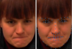
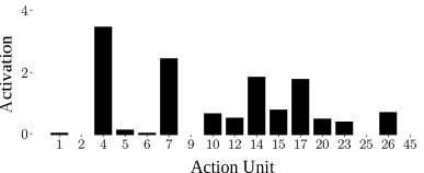
Figure 3: Facial expression with landmarks and AUs detected by OpenFace. Strong activation of AU 4 (brow lowerer), 7 (lid tightener), 14 (dimpler), and 17 (chin raiser)

s

3.3 Granger Causality

For the purpose of finding cause-effect relations, Granger’s concept of causality was used. GC is based on the axiom of temporal precedence, meaning that the past and present may cause the future, but the future cannot cause the past [Granger, 1980].

Let $\mathbf{x}_{t}=(x_{1},x_{2}\dots x_{z})_{t}$ and $\mathbf{y}_{t}=(y_{1},x_{2}\dots y_{z})_{t}$ be real-valued $z$-dimensional (column) vectors of AUs at time point $t$, $t=1\dots T$, and let $\bar{x}_{t}=\frac{1}{z}\sum_{i=1}^{z}(x_{i})_{t}$ and $\bar{y}_{t}=\frac{1}{z}\sum_{i=1}^{z}(y_{i})_{t}$ be the average of $\mathbf{x}_{t}$ and $\mathbf{y}_{t}$ at time point $t$. This results in two time series $\mathbf{X}_{t}=\bar{x}_{1},\dots\bar{x}_{T}$ and $\mathbf{Y}_{t}=\bar{y}_{1},\dots\bar{y}_{T}$ consisting of averaged values of AUs. For building the (averaged) GC model we require $\mathbf{X}_{t}$ and $\mathbf{Y}_{t}$ to be stationary.

The prediction of values of $\mathbf{X}$ and $\mathbf{Y}$ at time $t$ is based on previous values from $\mathbf{X}_{k}$ and $\mathbf{Y}_{k}$, $k<t$

$$\mathbf{X}_{t}=\sum_{j=1}^{m}a_{j}\mathbf{X}_{t-j}+\sum_{j=1}^{m}b_{j}\mathbf{Y}_{t-j}+\varepsilon_{t}\quad(1)$$

$$\mathbf{Y}_{t}=\sum_{j=1}^{m}c_{j}\mathbf{X}_{t-j}+\sum_{j=1}^{m}d_{j}\mathbf{Y}_{t-j}+\vartheta_{t}\quad(2)$$

with $\varepsilon_{t}$ and $\vartheta_{t}$ being two independent noise processes. For each expression of each participant in each condition we estimated the best model order $m$ using the Bayesian Information Criterion (BIC). For statistical significance, an F-Test with a level of significance of $p=0.05$ was used. When testing for GC three different cases regarding the direction of influence can occur [Schulze, 2004]:

1. If $a_{k}=0$ for $k=1\dots m$ and $\exists b_{k}\neq 0$ for $1\leq k\leq m$ then $\mathbf{Y}$ Granger causes $\mathbf{X}$.

2. If $d_{k}=0$ for $k=1\dots m$ and $\exists c_{k}\neq 0$ for $1\leq k\leq m$ then $\mathbf{X}$ Granger causes $\mathbf{Y}$.

3. If for both $\exists b_{k}\neq 0$ for $1\leq k\leq m$ and $\exists c_{k}\neq 0$ for $1\leq k\leq m$ holds a bidirectional (feedback) relation exists.

If none of the above cases holds, $\mathbf{X}$ and $\mathbf{Y}$ are not Granger causing each other. In our real data, we expected that, if present, pairs that do not Granger cause each other are rare.

3.4 Relevant Interval Selection

Considering the experimental setup, we had to expect multiple temporal scenes, further referred to as subintervals, in which the participants influenced each other. The time spans where causality is visible, might range from half a second to half a minute, occur several times, and can be interrupted by irrelevant scenes (e.g., one participant talking while the other participant is listening) that differ in the length of time. As outlined above, the direction of influence in a subinterval can either be bidirectional, or unidirectional driven by either S or R. This implies that three unwanted effects can occur, if the full time span is analysed: first, temporal relations are not found at all; second, bidirectional relations mask temporal unidirectional relations and; third, an unidirectional relation from $\mathbf{X}$ to $\mathbf{Y}$ masks temporal bidirectional influence or unidirectional influence from $\mathbf{Y}$ to $\mathbf{X}$. Li et al. [Li et al., 2017] give an example where temporal GC is not being detected, when the full time span is used for model fitting.

Our central idea is to apply GC only to time series obtained by concatenating highly coherent (e.g., in terms of Pearson correlation) subintervals of raw time series. Instead of using a brute force algorithm, we suggest using a bottom-up approach for finding the longest set of maximal, non-overlapping, correlated intervals in time series as proposed by Atluri et al. [Atluri et al., 2014]. The authors applied their approach to fMRI data where they achieved good results for clustering coherent working brain regions.

Let $\mathbf{X}_{t}$ and $\mathbf{Y}_{t}$ be two time series of length $N$. An interval is called correlated interval for a threshold $\beta$, when all its subintervals up to a lower interval length $\alpha$ are correlated as well. An interval $I_{(a,b)}$ from $a$ to $b$ is called maximal, when $I_{(a,b)}$ is a correlated interval, but $I_{(a-1,b)}$ and $I_{(a,b+1)}$ are not. And two intervals $I_{(a,b)}$ and $I_{(c,d)}$ are called non-overlapping, when $I_{(a,b)}\cap I_{(c,d)}=\emptyset$. From all intervals fulfilling these conditions the longest set (total length of intervals) is computed.

In a multivariate case (e.g., multiple AUs defining an expression), we propose to compute the longest set for each pair of corresponding variables and then use the intersection of intervals over all variables of the system, as selected relevant intervals. For further analysis, for each variable of the system the selected relevant intervals can be concatenated, resulting in multiple time series each composed of relevant information only. In the following we refer to the set of selected intervals between two time series $\mathbf{X}$ and $\mathbf{Y}$ as $AW_{XY}$.

3.5 Modeling Cause-Effect Relations

The two major challenges in the analysis of the cause-effect relations in dyadic dialogs, that make the application of conventional methods difficult were:

1. Due to the constructed situations, strong distinct emotions, computed by using traditional AU combinations, were rarely visible.

2. Time variant and situation-dependent communication, resulting in a high variety and volatility of time spans in which nonverbal cause-effect behavior between interacting partners is visible.

To tackle these difficulties, we use the combination of specific facial expressions and the relevant interval selection approch. The final selection of relevant intervals and the following analysis of causality for two systems of facial action units $\mathbf{x}_{1}\dots\mathbf{x}_{T}$ and $\mathbf{y}_{1}\dots\mathbf{y}_{T}$ consists of the following steps:

1. Calculate selected relevant intervals $AW_{x_{1t}y_{1t}},AW_{x_{2t}y_{2t}},\dots,AW_{x_{zt}y_{zt}}$ pairwise between corresponding system parameters.

2. Calculate the intersection $AW_{\mathbf{x}\mathbf{y}}$ of all sets of selected intervals $AW_{x_{1t}y_{1t}}\cap AW_{x_{2t}y_{2t}}\cap\dots\cap AW_{x_{zt}y_{zt}}$.

3. Concatenate selected intervals for each variable of $\mathbf{x}_{t}$ and $\mathbf{y}_{t}$

4. Compute GC on concatenation.

Before applying the relevant interval selection approach to our nonverbal communication data, we identified upper and lower facial expressions that changed significantly between the three experimental conditions. For that we calculated each participant’s average face, which is the average AU activation over the three conditions and used it as a lower threshold for the activation of an expression. That means, that we considered an expression as visible, when all of its associated AUs were greater than 0.5 standard deviations of the conspecific AUs in the average face. The number of activations per expression was counted per person and experimental condition, and normalized by video length and maximum count of the expression of each person. A Wilcoxon signed-rank test revealed, that the participants showed significantly more happiness in the respectful condition than in the contempt condition ($p=.034$, $s=92.0$). Further, we found both, more sadness lower ($p=.034$, $s=92.0$) and sadness upper ($p=.023,s=86.0$) expressions in the contempt condition compared to the objective condition, when using a Benjamini-Hochberg p-value correction [Benjamini and Hochberg, 1995] with a false discovery rate of $Q=.3$ and individual p-values of $\alpha=.5$.

As a next step, we applied the relevant interval selection approach, for computing selected intervals, pairwise to all of the identified AUs, with a minimum interval length of 75 and a threshold of 0.8 for Pearson correlation. Based on known average human reaction time (ca. 200 ms or 6 frames [Jain et al., 2015]), we shifted one time series by 0, 4, 8, and 12 frames both, back and forth in time, and computed relevant intervals. The grid selected for shifting does cover quicker and slower reactions of participants, while being computationally performant. Afterwards, we computed the longest set of the list of relevant intervals obtained from the different shifts. Before computing GC, we median filtered the selected intervals with a filter length of 51 (2 seconds). Finally, we calculated the average GC on the concatenation of the intervals in the set of selected intervals of the smoothed (Gaussian blur with $\sigma^{2}=1$, window size $20$) standardized time series. The results were counted according to the possible outcomes of the GC test in 3.3, as either unidirectional caused by S, unidirectional caused by R, bidirectional, or no causality.

4 EXPERIMENTAL RESULTS AND DISCUSSION

Evaluation on synthetic data. The following constructed example illustrates, how our idea contributes to a better detection of coherent subintervals in time series. Initially, we generated two time series of length $N=6000$, so that $\mathbf{X}_{t},\mathbf{Y}_{t}\sim{\mathcal{N}}(0,1)$, and $\mathbf{X}_{t}$, $\mathbf{Y}_{t}$ are independent. We then smoothed (Gaussian blur with $\sigma^{2}=1$, window size $10$) $\mathbf{X}$ and $\mathbf{Y}$. After that, multiple intervals of random length $l_{s}$, $l_{s}\sim{\mathcal{U}}(50,200)$ were synchronized and $\mathbf{Y}$ shifted by four samples back in time. A synchronized interval is followed by an unsynchronized interval of length $l_{u}$, $l_{u}\sim{\mathcal{U}}(100,600)$. In the last step, we added Gaussian noise $\epsilon$ to $Y$, $\epsilon\sim\mathcal{N}(0,0.02)$.

We expected the following approaches to detect all synchronized intervals, and identify the cause-effect relation on each interval in the manner that $\mathbf{Y}$ Granger causing $\mathbf{X}$, and no intervals for $\mathbf{X}$ Granger causing $\mathbf{Y}$, at different levels of significance $\alpha$. We compare the following two approaches:

1. Fixed size sliding window approach: For the fixed size sliding window approach we used window size $\gamma=50$ and step size $\nu=2$. Since multiple tests are performed, a Bonferroni corrected p-value $p_{f}=\frac{\alpha\nu}{2(n-\gamma)}$ was used for detecting GC.

2. Relevant interval selection approach: We set the minimum windows size to 50, the correlation threshold to $0.9$, and used a two-sided time shift of 4. The Bonferroni corrected p-value $p_{aw}=\frac{\alpha}{2\left|{AW_{XY}}\right|}$ was selected according to the number of intervals $\left|{AW_{XY}}\right|$ detected by the relevant interval selection approach.

For $\mathbf{Y}$ Granger causing $\mathbf{X}$, we evaluated precision and recall with the synchronized intervals as ground truth. For $\mathbf{X}$ Granger causing $\mathbf{Y}$, the ground truth is the full time series, and thus, only recall needs to be evaluated. Figure 4 shows the evaluation for $\mathbf{Y}$ Granger causing $\mathbf{X}$. Both approaches show a very good performance in detecting all relevant intervals (recall). Yet, the relevant interval selection approach detects less irrelevant intervals (precision) among all levels of significance. Figure 5 shows that both, relevant interval selection and fixed size sliding window approach, show a very high recall for $\mathbf{X}$ Granger causing $\mathbf{Y}$ among all levels of significance, but the relevant interval selection approach is slightly superior.

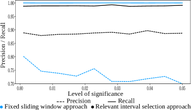
Figure 4: Precision and recall for relevant interval selection and fixed size sliding window approaches for $\mathbf{Y}$ Granger causing $\mathbf{X}$.

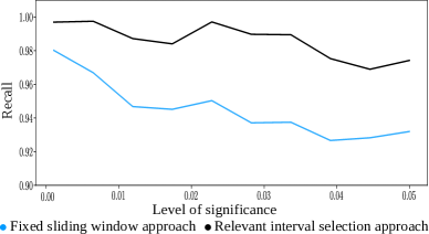
Figure 5: Recall for relevant interval selection and fixed size sliding window approaches for $\mathbf{X}$ Granger causing $\mathbf{Y}$.

Evaluation on nonverbal communication data. In Figure 6, our relevant interval selection approach is compared to the full time span approach. The figure shows the percentage of pairs for which the GC test, with $p=0.05$, showed a specific direction of influence, under the three experimental conditions, for each of the identified expressions (sadness lower, sadness upper, happiness). Especially for sadness lower and sadness upper expressions, the full time span approach does not find causality between S and R for over 50% of the pairs. With our relevant interval selection approach, less pairs show no causality, but instead uni- or bidirectional causation. Especially in the sadness lower condition, we were able to detect that the direction of influence was more often driven by S or bidirectional, and rarely driven by R. The full time span approach does not expose this information at all. In the contempt condition S is not supposed to show positive expressions.

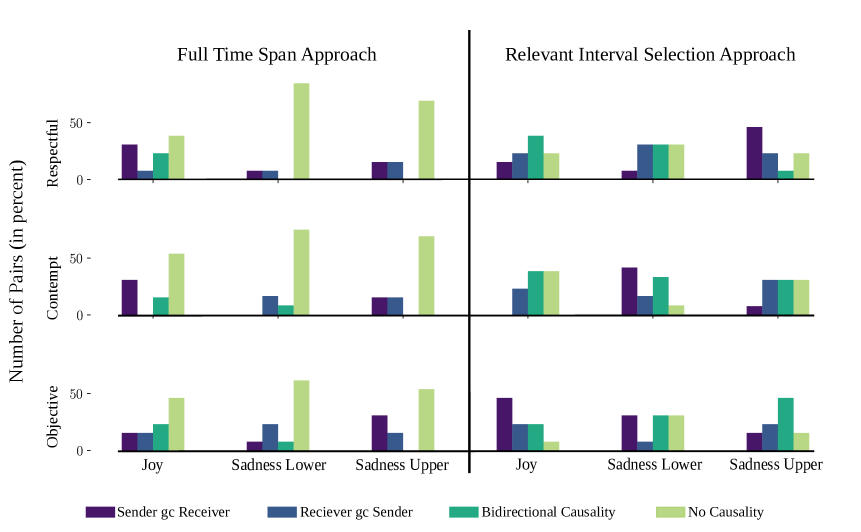
Figure 6: Relevant interval selection approach compared to full time span approach for different facial expressions under the three experimental conditions for distinguishing the direction of influence.

5 CONCLUSIONS

In this paper, we employed GC together with a relevant interval selection approach on synthetic and nonverbal communication data obtained from an experimental setup. Based on the results of Wegrzyn et al. [Wegrzyn et al., 2017] we designed our own emotional facial features, capable of capturing emotions even when strong distinct emotions are not visible. Our facial expressions are composed of facial action units, which can be detected by real-time, state of the art computer vision tools. We proposed an intelligent interval selection approach for filtering relevant information in dyadic dialogs. Subsequently, we were able to apply our GC model to the concatenation of relevant intervals and compute the direction of influence.

We applied our approach to real data. On the one hand, this emphasised the superiority of the relevant interval selection approach compared to a full time span approach and on the other hand, this revealed that in contemptuous dyadic dialogs happiness was more often caused by R whereas sadness lower was more often initiated by S- a pattern of results which was theoretically to be expected. In general many bidirectional influences were found.

As no standardized mapping from AUs to emotions exists, we proposed using a system of upper and lower facial expressions. For further research, we suggest using a learning system, capable of classifying upper and lower emotions based on all AUs.

In our approach we used correlation which is a linear similarity measure. For nonlinear dependence, Pearson correlation can be easily replaced by appropriate distance measures such as mutual information. The GC model must be changed accordingly.

Overall, we identify our contribution as an important step towards interdisciplinary, with computer vision potentials, psychological observations, and theoretical knowledge of causality methods being combined and extended to gain interesting insights into emotional social interaction.

REFERENCES

- Atluri et al., 2014 Atluri, G., Steinbach, M., Lim, K., MacDonald, A., and Kumar, V. (2014). Discovering the longest set of distinct maximal correlated intervals in time series data.
- Baltrušaitis et al., 2015 Baltrušaitis, T., Mahmoud, M., and Robinson, P. (2015). Cross-dataset learning and person-specific normalisation for automatic action unit detection. In Automatic Face and Gesture Recognition (FG), 2015 11th IEEE International Conference and Workshops on, volume 6, pages 1–6. IEEE.
- Baltrusaitis et al., 2018 Baltrusaitis, T., Zadeh, A., Lim, Y. C., and Morency, L.-P. (2018). Openface 2.0: Facial behavior analysis toolkit. In Automatic Face & Gesture Recognition (FG 2018), 2018 13th IEEE International Conference on, pages 59–66. IEEE.
- Benjamini and Hochberg, 1995 Benjamini, Y. and Hochberg, Y. (1995). Controlling the false discovery rate: a practical and powerful approach to multiple testing. Journal of the royal statistical society. Series B (Methodological), pages 289–300.
- Bousmalis et al., 2013 Bousmalis, K., Mehu, M., and Pantic, M. (2013). Towards the automatic detection of spontaneous agreement and disagreement based on nonverbal behaviour: A survey of related cues, databases, and tools. Image and Vision Computing, 31(2):203–221.
- Burgoon et al., 2016 Burgoon, J. K., Guerrero, L. K., and Floyd, K. (2016). Nonverbal communication. Routledge.
- Cohn et al., 2007 Cohn, J. F., Ambadar, Z., and Ekman, P. (2007). Observer-based measurement of facial expression with the facial action coding system. The handbook of emotion elicitation and assessment, pages 203–221.
- Ding et al., 2006 Ding, M., Chen, Y., and Bressler, S. L. (2006). Granger causality: basic theory and application to neuroscience. Handbook of time series analysis: recent theoretical developments and applications, pages 437–460.
- Ekman, 1992 Ekman, P. (1992). An argument for basic emotions. Cognition & emotion, 6(3-4):169–200.
- Ekman, 2002 Ekman, P. (2002). Facial action coding system (facs). A human face.
- Ekman and Friesen, 1978 Ekman, P. and Friesen, W. (1978). Facial action coding system: A technique for the measurement of facial action. Manual for the Facial Action Coding System.
- Ekman and Rosenberg, 1997 Ekman, P. and Rosenberg, E. L. (1997). What the face reveals: Basic and applied studies of spontaneous expression using the Facial Action Coding System (FACS). Oxford University Press, USA.
- El Kaliouby and Robinson, 2005 El Kaliouby, R. and Robinson, P. (2005). Real-time inference of complex mental states from facial expressions and head gestures. In Real-time vision for human-computer interaction, pages 181–200. Springer.
- Granger, 1980 Granger, C. (1980). Testing for causality: A personal viewpoint. Journal of Economic Dynamics and Control, 2:329 – 352.
- Granger et al., 2000 Granger, C. W., Huangb, B.-N., and Yang, C.-W. (2000). A bivariate causality between stock prices and exchange rates: evidence from recent asianflu☆. The Quarterly Review of Economics and Finance, 40(3):337–354.
- Jain et al., 2015 Jain, A., Bansal, R., Kumar, A., and Singh, K. (2015). A comparative study of visual and auditory reaction times on the basis of gender and physical activity levels of medical first year students. International Journal of Applied and Basic Medical Research, 5(2):124.
- Kalimeri et al., 2012 Kalimeri, K., Lepri, B., Aran, O., Jayagopi, D. B., Gatica-Perez, D., and Pianesi, F. (2012). Modeling dominance effects on nonverbal behaviors using granger causality. In Proceedings of the 14th ACM international conference on Multimodal interaction, pages 23–26. ACM.
- Kalimeri et al., 2011 Kalimeri, K., Lepri, B., Kim, T., Pianesi, F., and Pentland, A. S. (2011). Automatic modeling of dominance effects using granger causality. In International Workshop on Human Behavior Understanding, pages 124–133. Springer.
- Langner et al., 2010 Langner, O., Dotsch, R., Bijlstra, G., Wigboldus, D. H., Hawk, S. T., and Van Knippenberg, A. (2010). Presentation and validation of the radboud faces database. Cognition and emotion, 24(8):1377–1388.
- Li et al., 2017 Li, Z., Zheng, G., Agarwal, A., Xue, L., and Lauvaux, T. (2017). Discovery of causal time intervals. In Proceedings of the 2017 SIAM International Conference on Data Mining, pages 804–812. SIAM.
- Matsuyama et al., 2016 Matsuyama, Y., Bhardwaj, A., Zhao, R., Romeo, O., Akoju, S., and Cassell, J. (2016). Socially-aware animated intelligent personal assistant agent. In Proceedings of the 17th Annual Meeting of the Special Interest Group on Discourse and Dialogue, pages 224–227.
- Schneider et al., 2017 Schneider, D., Glaser, M., and Senju, A. (2017). Autism spectrum disorder. In V. Zeigler-Hill, T.K. Shackelford (Eds.), Encyclopedia of Personality and Individual Differences. Springer International Publishing AG.
- Schulze, 2004 Schulze, P. M. (2004). Granger-kausalitätsprüfung: Eine anwendungsorientierte darstellung. Technical report, Arbeitspapier/Institut für Statistik und Ökonometrie, STATOEK.
- Sheerman-Chase et al., 2009 Sheerman-Chase, T., Ong, E.-J., and Bowden, R. (2009). Feature selection of facial displays for detection of non verbal communication in natural conversation. In Computer Vision Workshops (ICCV Workshops), 2009 IEEE 12th International Conference on, pages 1985–1992. IEEE.
- Wegrzyn et al., 2017 Wegrzyn, M., Vogt, M., Kireclioglu, B., Schneider, J., and Kissler, J. (2017). Mapping the emotional face. how individual face parts contribute to successful emotion recognition. PloS one, 12(5):e0177239.
- Zhang et al., 2011 Zhang, D. D., Lee, H. F., Wang, C., Li, B., Pei, Q., Zhang, J., and An, Y. (2011). The causality analysis of climate change and large-scale human crisis. Proceedings of the National Academy of Sciences, page 201104268.