Computation and stability of waves
in equivariant evolution equations

Wolf-Jürgen Beyn^,           Denny Otten^,
Department of Mathematics, Bielefeld University

33501 Bielefeld, Germany

Date: March 8, 2024

Abstract.

Travelling and rotating waves are ubiquitous phenomena observed in time dependent PDEs modelling the combined effect of dissipation and non-linear interaction. From an abstract viewpoint they appear as relative equilibria of an equivariant evolution equation. In numerical computations the freezing method takes advantage of this structure by splitting the evolution of the PDE into the dynamics on the underlying Lie group and on some reduced phase space. The approach raises a series of questions which were answered to a certain degree by the project: linear stability implies non-linear (asymptotic) stability, persistence of stability under discretisation, analysis and computation of spectral structures, first versus second order evolution systems, well-posedness of partial differential algebraic equations, spatial decay of wave profiles and truncation to bounded domains, analytical and numerical treatment of wave interactions, relation to connecting orbits in dynamical systems. A further numerical problem related to this topic will be discussed, namely the solution of non-linear eigenvalue problems via a contour method.

Key words. Equivariant evolution equations, relative equilibria, freezing method, rotating and traveling waves, asymptotic stability, reaction-diffusion systems, Hamiltonian PDEs, nonlinear eigenvalue problems.

AMS subject classification. 37Lxx, 65J08, 74J30, 65L15, 35B40.

1. Equivariant Evolution Equations

1.1. Abstract Setting

The overall topic of the project is the numerical analysis of evolution equations which may be written in the abstract form

(1.1) $$u_{t}=F(u),\quad t\geq 0,$$

where the solution $u:[0,T)\rightarrow X$, $t\mapsto u(t)$ is defined on a real interval $[0,T),0<T\leq\infty$ has values in a Banach space $X$, and time derivative $u_{t}$. The map $F:Z\subseteq X\rightarrow X$ is a vector field defined on a dense subspace $Z$ of $X$. The additional structure is described in terms of a Lie group $G$ of dimension $n=\dim(G)<\infty$ which acts on $X$ via a homomorphism into the general linear group $GL(X)$ of homeomorphisms on $X$:

(1.2) $$a:G\rightarrow GL(X),\quad\gamma\mapsto a(\gamma).$$

For the images we use the synonymous notation $a(g)u=a(g,u),g\in G,u\in X$.

We assume that equation (1.1) is equivariant with respect to this group action, i.e. the vector field $F$ has the following property

(1.3) $$F(a(\gamma)u)=a(\gamma)F(u)\quad\forall\gamma\in G\;\forall u\in Z,$$

where we have assumed $a(\gamma)Z\subseteq Z$ for all $\gamma\in G$.

In Sections 2.2 and 3 we will deal with several classes of partial differential equations which fit into this general setting. All of them are formulated for functions on a Euclidean space $\mathbb{R}^{d}$ where the action is caused by the special Euclidean group $SE(d)$ acting via rotations and translations on their arguments or on their values.

Remark 1.1.

For some applications even this framework is not sufficient. For example, travelling fronts which have finite but non-zero limits at infinity, do not lie in any of the usual Lesbesgue or Sobolev spaces, but in an affine space. To cover such cases, but also more general PDEs on manifolds, one can generalise the whole approach to Banach manifolds $X$, where $F$ is a vector field defined on a submanifold $Z$ of $X$ mapping into the tangent bundle $TX$, and $a$ takes values in the space of diffeomorphisms $\mathrm{Diff}(X,X)$. Equivariance (1.3) is then expressed as $F(a(\gamma,u))=d_{u}[a(\gamma,u)]F(u)$, where $d_{u}[a(\gamma,u)]:T_{u}X\rightarrow T_{a(\gamma,u)}X$ denotes the tangent map. For the sake of simplicity we will not pursue this generalisation here (see [47]).

For this article it is sufficient to work with a simple notion of a strong solution of a Cauchy problem instead of dealing with weak solutions in time and mild solutions in space.

Definition 1.2.

A function $u\in C^{1}([0,T),X)\cap C([0,T),Z)$ satisfying

(1.4) $$u_{t}=F(u),t\in[0,T),\quad u(0)=u_{0}\in Z,$$

is called a strong solution of the Cauchy problem (1.4).

In the following we will always assume that a strong solution of (1.4) exists locally, i.e. on some interval $[0,T),T>0$, and that it is unique. For applications to PDEs it is typical that the group action is only differentiable for smooth functions. Therefore, we impose the following condition.

Assumption 1.3.

For any $u\in X$, resp. $u\in Z$ the mapping

$$a(\cdot)u:G\rightarrow X,\quad\gamma\mapsto a(\gamma)u$$

is continuous resp. continuously differentiable with derivative

(1.5) $$d_{\gamma}[a(\gamma)u]:T_{\gamma}G\rightarrow X,\quad\mu\mapsto d_{\gamma}[a(\gamma)u]\mu.$$

In case $\gamma=\mathbbm{1}$ the tangent space $T_{\mathbbm{1}}G$ may be identified with the Lie algebra $\mathfrak{g}$ of $G$, and we have $d_{\gamma}[a(\mathbbm{1})u]:\mathfrak{g}\rightarrow X$.

1.2. Relative Equilibria

Relative equilibria are special solutions of (1.1) which lie in the group orbit of a single element.

Definition 1.4.

A pair $v_{\star}\in Z,\gamma_{\star}\in C^{1}([0,\infty),G)$ is called a relative equilibrium of (1.1) if $\gamma_{\star}(0)=\mathbbm{1}$ and $u_{\star}(t)=a(\gamma_{\star}(t))v_{\star},t\geq 0$ is a strong solution of (1.4) with $u_{0}=v_{\star}$.

In some references (see e.g. [19]) the whole group orbit $\mathcal{O}_{G}(v_{\star})=\{a(g)v_{\star}:g\in G\}$ is called a relative equilibrium. However, we include the path $t\rightarrow\gamma_{\star}(t)$ on the group as part of our definition since it will be relevant for both the stability analysis and numerical computations. The following theorem shows that the path may always be written as $\gamma_{\star}(t)=\exp(t\mu_{\star})$ for some $\mu_{\star}\in\mathfrak{g}$. Recall that $\exp:\mathfrak{g}\rightarrow G$ is the exponential function and that $\gamma_{\star}(t)=\exp(t\mu_{\star}),t\in\mathbb{R}$ is the unique solution of the Cauchy problem

(1.6) $$\gamma_{\star}^{\prime}(t)=dL_{\gamma_{\star}(t)}(\mathbbm{1})\mu_{\star},\quad\gamma_{\star}(0)=\mathbbm{1},$$

where $L_{\gamma}g=\gamma\circ g,g\in G$ denotes the multiplication by $\gamma$ from the left. The vector field on the right-hand side of (1.6) is often simply written as $\gamma_{\star}(t)\mu_{\star}$, but in analogy to (1.5) we keep the slightly clumsier notation $dL_{\gamma_{\star}(t)}(\mathbbm{1})\mu_{\star}$ for clarity.

Theorem 1.5.

Let Assumption 1.3 hold. Then for every relative equilibrium $v_{\star}\in Z,\gamma_{\star}\in C^{1}([0,\infty),G)$ there exists $\mu_{\star}\in\mathfrak{g}$ such that

(1.7) $$0= F(v_{\star})-d_{\gamma}[a(\mathbbm{1})v_{\star}]\mu_{\star}$$

(1.8) $$a(\gamma_{\star}(t))v_{\star}= a(\exp(t\mu_{\star}))v_{\star}.$$

Conversely, let $v_{\star}\in Z,\mu_{\star}\in\mathfrak{g}$ solve (1.7), then $v_{\star}$ and $\gamma_{\star}(t)=\exp(t\mu_{\star}),t\geq 0$ are a relative equilibrium.

Given $v_{\star}$ and $\gamma_{\star}(\cdot)$, then uniqueness of $\mu_{\star}$ will follow from (1.8) in the first part of the theorem if the stabiliser $H(v_{\star})$ of $v_{\star}$ is simple, i.e.

(1.9) $$H(v_{\star})=\{\gamma\in G:a(\gamma)v_{\star}=v_{\star}\}=\{\mathbbm{1}\}.$$

But even then, equation (1.7) does not determine the pair $(v_{\star},\mu_{\star})$ uniquely, since relative equilibria always come in families. More precisely, Definition 1.4 and the equivariance (1.3) show that any relative equilibrium $v_{\star},\gamma_{\star}$ of (1.4) is accompanied by a family $(w(g),\gamma(g,\cdot)),g\in G$ of relative equilibria given by

(1.10) $$w(g)=a(g)v_{\star},\quad\gamma(g,t)=g\circ\gamma_{\star}(t)\circ g^{-1},\quad g\in G,$$

see [18] for related results. This will be important for the stability analysis in Section 4.

1.3. Wave Solutions of PDEs

Two important classes of semi-linear evolution equations which fit into the above setting and to which our results apply, are the following

(1.11) $$u_{t}=Au_{xx}+f(u,u_{x}),\quad u(x,t)\in\mathbb{R}^{m},\quad x\in\mathbb{R},t\geq 0,\quad u(\cdot,0)=u_{0},$$

(1.12) $$u_{t}=A\Delta u+f(u),\quad u(x,t)\in\mathbb{R}^{m},\quad x\in\mathbb{R}^{d},t\geq 0,\quad u(\cdot,0)=u_{0}.$$

In both cases $A\in\mathbb{R}^{m,m}$ is assumed to have spectrum $\sigma(A)$ with $\operatorname{Re}(\sigma(A))\geq 0$. Note that $\operatorname{Re}(\sigma(A))>0$ leads to parabolic systems while $\sigma(A)\subseteq i\mathbb{R}$ occurs for Hamiltonian PDEs. Intermediate cases with $\sigma(A)\subset(\{0\}\cup\{\operatorname{Re}z>0\})$ generally belong to hyperbolic or parabolic-hyperbolic mixed systems. The non-linearities $f:\mathbb{R}^{2m}\rightarrow\mathbb{R}^{m}$ in (1.11) resp. $f:\mathbb{R}^{m}\rightarrow\mathbb{R}^{m}$ in (1.12) are assumed to be sufficiently smooth and to satisfy $f(0,0)=0$ resp. $f(0)=0$.

In case of (1.11) the Lie group is $(G,\circ)=(\mathbb{R},+)$ acting on $X=L^{2}(\mathbb{R},\mathbb{R}^{m})$ by the shift $[a(\gamma)u](x)=u(x-\gamma),x\in\mathbb{R},u\in X$. With $F(u)=Au_{xx}+f(u,u_{x})$ for $u\in Z=H^{2}(\mathbb{R},\mathbb{R}^{m})$, equivariance is easily verified and $F(u)\in X$ follows from the Sobolev embedding $H^{1}(\mathbb{R},\mathbb{R}^{m})\subseteq L^{\infty}(\mathbb{R},\mathbb{R}^{m})$ and $f(0,0)=0$. For the derivative we find

$$d_{\gamma}[a(\mathbbm{1})v]\mu=-v_{x}\mu,\quad\mu\in\mathfrak{g}=\mathbb{R},\quad v\in H^{1}(\mathbb{R},\mathbb{R}^{m}).$$

Relative equilibria then turn out to be travelling waves

(1.13) $$u_{\star}(x,t)=v_{\star}(x-\mu_{\star}t),x\in\mathbb{R},t\geq 0,$$

where the pair $(v_{\star},\mu_{\star})$ solves the second order system from (1.7)

$$0=Av_{\star,\xi\xi}+\mu_{\star}v_{\star,\xi}+f(v_{\star},v_{\star,\xi}),\quad v(\xi)\in\mathbb{R}^{m},\xi\in\mathbb{R}.$$

In fact, our simplified abstract approach only covers pulse solutions (defined by $v_{\star}(\xi),v_{\star,\xi}(\xi)\rightarrow 0$ as $\xi\rightarrow\pm\infty$), whereas fronts need the setting of manifolds, see Remark 1.1.

In the multi-dimensional case (1.12) the phase space is $X=L^{2}(\mathbb{R}^{d},\mathbb{R}^{m})$, and we aim at equivariance w.r.t. the special Euclidean group $G=\mathrm{SE}(d)=\mathrm{SO}(d)\ltimes\mathbb{R}^{d}$. It is convenient to represent $\mathrm{SE}(d)$ in $GL(\mathbb{R}^{d+1})$ as

(1.14) $$\mathrm{SE}(d)=\left\{\begin{pmatrix}Q&b\\ 0&1\end{pmatrix}:Q\in\mathbb{R}^{d,d},Q^{\top}Q=I_{d},\det(Q)=1,b\in\mathbb{R}^{d}\right\},$$

where the group operation is matrix multiplication. We represent the Lie algebra $\mathfrak{se}(d)=\mathfrak{so}(d)\times\mathbb{R}^{d}$ accordingly

(1.15) $$\mathfrak{se}(d)=\left\{\begin{pmatrix}S&a\\ 0&0\end{pmatrix}:S\in\mathbb{R}^{d,d},S^{\top}=-S,a\in\mathbb{R}^{d}\right\}.$$

The action on functions $u\in X$ is defined by

$$[a(\gamma)u](x)=u(Q^{\top}(x-b)),\quad x\in\mathbb{R}^{d},\gamma=\begin{pmatrix}Q&b\\ 0&1\end{pmatrix}\in\mathrm{SE}(d).$$

The derivative exists for functions $u\in H^{1}_{\mathrm{Eucl}}(\mathbb{R}^{d},\mathbb{R}^{m})$ where for $k\geq 1$

$$H^{k}_{\mathrm{Eucl}}(\mathbb{R}^{d},\mathbb{R}^{m})=\left\{u\in H^{k}(\mathbb{R}^{d},\mathbb{R}^{m}):\mathcal{L}_{S}u\in L^{2}(\mathbb{R}^{d},\mathbb{R}^{m})\;\forall S\in\mathfrak{so}(d)\right\},$$

and

$$L_{S}u(x):=u_{x}(x)Sx=\sum_{j,k=1}^{d}D_{j}u(x)S_{j,k}x_{k},\quad x\in\mathbb{R}^{d}.$$

The derivative of the group action is then given by

$$\left(d_{\gamma}[a(\mathbbm{1})v]\mu\right)(x)=-v_{x}(x)(Sx+c),\quad x\in\mathbb{R}^{d},\quad\mu=\begin{pmatrix}S&c\\ 0&0\end{pmatrix}\in\mathfrak{se}(d).$$

Note that the first order operator $\mathcal{L}_{S}$ has unbounded coefficients and that the norm in $H^{k}_{\mathrm{Eucl}}$ is given by

$$\|u\|^{2}_{H^{k}_{\mathrm{Eucl}}}=\|u\|^{2}_{H^{k}}+\sup\{\|\mathcal{L}_{S}u\|^{2}_{L^{2}}:S\in\mathfrak{so}(d),|S|=1\}.$$

Setting $Z=H^{2}_{\mathrm{Eucl}}(\mathbb{R}^{d},\mathbb{R}^{m})$ one finds $F(u)=A\Delta u+f(u)\in X$ for $u\in Z$ in dimension $d=2$, since $H^{2}(\mathbb{R}^{2},\mathbb{R}^{m})\subset L^{\infty}(\mathbb{R}^{2},\mathbb{R}^{m})$ by Sobolev embedding. But for $d\geq 3$ one has to impose growth conditions on $f$ to ensure this. Equivariance follows from the equivariance of the Laplacian under Euclidean transformations. Special types of relative equilibria are waves rotating about a centre $x_{\star}\in\mathbb{R}^{d}$:

(1.16) $$u_{\star}(x,t)=v_{\star}(\exp(-tS_{\star})(x-x_{\star})),\quad v_{\star}\in Z,S_{\star}\in\mathfrak{so}(d).$$

When substituting $\xi=\exp(-tS_{\star})(x-x_{\star})$ the system (1.7) reads

$$0=A\Delta v_{\star}+v_{\star,\xi}S_{\star}\xi+f(v_{\star}),\quad\xi\in\mathbb{R}^{d}.$$

Several examples of travelling and rotating waves will be dealt with in Section 3.

2. The Freezing Method

2.1. The abstract approach

The idea of the freezing method, set out in [53],[14], is to separate the strong solutions of the Cauchy problem (1.4) into a motion on the group $G$ and on a reduced phase space, just as for the relative equilibria in Definition 1.4:

(2.1) $$u(t)=a(\gamma(t))v(t),\quad t\geq 0.$$

Let $\gamma\in C^{1}([0,T),G),\gamma(0)=\mathbbm{1}$ and let $u$ be a strong solution of (1.4) and define $\mu(t):=(dL_{\gamma(t)}(\mathbbm{1}))^{-1}\gamma_{t}(t)\in\mathfrak{g}$ in the Lie algebra $\mathfrak{g}$ of $G$, then $\gamma,v$ solve the system

(2.2) $$v_{t}(t)= F(v(t))-d_{\gamma}[a(\mathbbm{1})v(t)]\mu(t), v(0)=u_{0},$$

(2.3) $$\gamma_{t}(t)= dL_{\gamma(t)}(\mathbbm{1})\mu(t), \gamma(0)=\mathbbm{1}.$$

Conversely, one can show that a strong solution $u\in C^{1}([0,T),X)\cap C([0,T),Z)$, $\mu\in C([0,T),\mathfrak{g})$, $\gamma\in C^{1}([0,T),G)$ of (2.2),(2.3) leads to a strong solution of (1.4) via (2.1). According to Theorem 1.5 a relative equilibrium $v_{\star},\mu_{\star}$ of (1.1) is a steady state of the first equation (2.2). Following [53], we call equation (2.3) the reconstruction equation. Due to the extra variables $\gamma\in G$ resp. $\mu\in\mathfrak{g}$, the system (2.2), (2.3) is not yet well posed, but needs $n=\dim(G)$ additional algebraic constraints (called phase conditions) which we write as

(2.4) $$\psi(v,\mu)=0.$$

Here $\psi:X\times\mathfrak{g}\rightarrow\mathfrak{g}^{\star}$ (the dual of $\mathfrak{g}$) is a smooth map typically derived as a necessary condition from a minimisation principle. For example, if $(X,\langle\cdot,\cdot\rangle)$ is a Hilbert space one can require the distance $\inf_{g\in G}\|v-a(g)\hat{v}\|$ to the group orbit of a template function $\hat{v}\in X$ (such as $\hat{v}=u_{0}$) to be minimal at $g=\mathbbm{1}$. For $\hat{v}\in Z$ this leads to the fixed phase condition

(2.5) $$\psi_{\mathrm{fix}}(v,\mu)\nu=\langle d_{\gamma}[a(\mathbbm{1})\hat{v}]\nu,v-\hat{v}\rangle=0,\quad\forall\nu\in\mathfrak{g}.$$

An alternative is to minimise $\|v_{t}\|^{2}=\|F(v)-d_{\gamma}[a(\mathbbm{1})v]\mu\|^{2}$ with respect to $\mu$ at each time instance, resulting in the orthogonality condition

(2.6) $$\psi_{\mathrm{orth}}(v,\mu)\nu=\langle d_{\gamma}[a(\mathbbm{1})v]\nu,F(v)-d_{\gamma}[a(\mathbbm{1})v]\mu\ \rangle=0\quad\forall\nu\in\mathfrak{g}.$$

This condition requires the group orbit of $v(t)$ to be tangent to its time derivative at each time instance. Altogether, equations (2.2) and (2.4) constitute a partial differential algebraic equation (PDAE) for the functions $v$ and $\mu$. The reconstruction equation (2.3) decouples from the PDAE and may be solved in a post-processing step. Condition (2.6) has a unique solution $\mu$ if $d_{\gamma}[a(\mathbbm{1})v]:\mathfrak{g}\rightarrow X$ is one to one and then leads to a PDAE of (differentiation) index $1$. Condition (2.5) leads to an index $2$ problem, but can be reduced to index $1$ by differentiating with respect to $t$ and then inserting (2.2).

2.2. Application to Evolution Equations

In this section we take a closer look at the PDAEs that arise from the freezing method when applied to the two equations (1.11) and (1.12). In Section 3 we will provide a series of numerical examples and also discuss the influence of both spatial and temporal discretisation errors. In the following we restrict to the fixed phase condition (2.5) which is particularly well-suited near a relative equilibrium and which admits rather general stability results, see Section 4. On the other hand the orthogonal phase condition needs no pre-information and hence can be applied far away from any relative equilibrium. However, its stability properties are questionable and have only been investigated in a special case, see [15].

For the one-dimensional system (1.11) with shift equivariance the freezing ansatz simply reads

(2.7) $$u(x,t)=v(x-\gamma(t),t),\quad x\in\mathbb{R},t\geq 0,\quad\mu(t)=\gamma_{t}(t),$$

and the corresponding PDAE is given by (cf. [59])

(2.8) $$v_{t} =Av_{\xi\xi}+\mu v_{\xi}+f(v,v_{\xi}), v(\cdot,0)=u_{0},$$

$$0 =\langle\hat{v}_{\xi},v-\hat{v}\rangle_{L^{2}(\mathbb{R},\mathbb{R}^{m})},$$

$$\gamma_{t} =\mu, \gamma(0)=0,$$

for the unknown quantities $(v,\mu,\gamma)$. For initial data $u_{0}$ close to a wave we expect $v(\cdot,t)\to v_{\star}$, $\mu(t)\to\mu_{\star}$ as $t\to\infty$. Travelling waves in parabolic systems and their stability are analysed in [35, 55, 62, 59], and numerical applications of the freezing method for this case appear in in [10].

Next, consider the parabolic system (1.12) in several space dimensions. With the special Euclidean group (1.14) and its Lie algebra (1.15) the freezing system (2.2),(2.3) takes the form

(2.9) $$v_{t} =Av_{\xi\xi}+v_{\xi}(S\xi+c)+f(v), v(\cdot,t_{0})=u_{0},$$

$$0 =\langle\xi_{j}\hat{v}_{\xi_{i}}-\xi_{i}\hat{v}_{\xi_{j}},v-\hat{v}\rangle_{L^{2}}, 0=\langle\hat{v}_{\xi_{l}},v-\hat{v}\rangle_{L^{2}},$$

$$\left(\begin{smallmatrix}Q&b\\ 0&1\end{smallmatrix}\right)_{t} =\left(\begin{smallmatrix}Q&b\\ 0&1\end{smallmatrix}\right)\left(\begin{smallmatrix}S&c\\ 0&0\end{smallmatrix}\right), \left(\begin{smallmatrix}Q(t_{0})&b(t_{0})\\ 0&1\end{smallmatrix}\right)=I_{d+1},$$

for the unknown quantities $\left(v,\mu=\left(\begin{smallmatrix}S&c\\ 0&0\end{smallmatrix}\right),\gamma=\left(\begin{smallmatrix}Q&b\\ 0&1\end{smallmatrix}\right)\right)$ and indices $1\leq i<j\leq d$, $1\leq l\leq d$. Since $S(t)$ is skew-symmetric it is sufficient to work with $S_{ij}$, $i=1,\ldots,d-1$, $j=i+1,\ldots,d$ and $c\in\mathbb{R}^{d}$ when solving the reconstruction equation. Numerical methods for differential equations on Lie groups may be found in [34]. If the initial data are close to a stable rotating wave (1.16) we expect $v(\cdot,t)\to v_{\star}$ and $\left(\begin{smallmatrix}S&c\\ 0&0\end{smallmatrix}\right)=\mu(t)\to\mu_{\star}=\left(\begin{smallmatrix}S_{\star}&c_{\star}\\ 0&0\end{smallmatrix}\right)\in\mathrm{se}(d)$ as $t\to\infty$. Rotating waves in parabolic systems are treated in [25, 26], their non-linear stability (for $d=2$) in [6], and numerical examples in [43]. Essential steps for extending non-linear stability to higher space dimensions are done in [7, 8, 9], which is based on previous works [43, 44, 45, 46].

2.3. Dynamic Decomposition of Multi-Waves

Consider a simplified parabolic system (1.11) in one space dimension

(2.10) $$u_{t}=Au_{xx}+f(u), u(\cdot,0)=u_{0},$$

under the assumptions of Section 1.3. Suppose this system admits several travelling waves $(v_{\star,j},\mu_{\star,j}),j=1,\ldots,N$ with different speeds $\mu_{\star,j}$ and limit behaviour $\lim_{\xi\to\pm\infty}v_{\star,j}(\xi)=v_{j}^{\pm}$ for $j=1,\ldots,N$. If the limits fit together, i.e. if

$$v^{+}_{j}=v^{-}_{j+1},\quad j=1,\ldots,N-1,$$

then one often observes $N$-waves (or multi-waves) of (2.10) which look like linear superpositions of the waves $v_{\star,j}(x-\mu_{\star,j}t),j=1,\ldots,N$, see for example Figures 3.6, 3.6 for two fronts from example (3.1) travelling at different speeds to the left and superimposed onto each other. Strong interaction occurs when two or several fronts move towards each other, while all other cases are called weak interactions. Many more interaction phenomena of this type may be found in [63] and the references therein.

In [10, 57] we extend the freezing method in order to handle such interactions. More precisely, we generalise (2.7) to

(2.11) $$u(x,t)=\sum_{j=1}^{N}v_{j}(x-\gamma_{j}(t),t),$$

where the values of $\gamma_{j}:\mathbb{R}\rightarrow\mathbb{R}$ denote the time-dependent position of the $j$-th profile $v_{j}:\mathbb{R}\rightarrow\mathbb{R}^{m}$ which we expect to have limits

$$\lim_{\xi\rightarrow\pm\infty}v_{j}(\xi,t)=v_{j}^{\pm}-w_{j}^{-},\quad w_{j}^{-}=\begin{cases}0,&j=1,\\ v_{j}^{-}&j\geq 2.\end{cases}$$

The main idea is to combine (2.11) with a dynamic partition of unity

$$Q_{j}(\gamma(t),x)=\frac{\varphi(x-\gamma_{j}(t))}{\sum_{k=1}^{N}\varphi(x-\gamma_{k}(t))},\quad j=1,\ldots,N,$$

where $\varphi\in C^{\infty}(\mathbb{R},(0,1])$ is a mollifier function, for example $\varphi(x)=\mathrm{sech}(\beta x)$ for some $\beta>0$. Using (2.11) in (2.10) and abbreviating $v_{k}(\star)=v_{k}(\cdot-\gamma_{k}(t),t)$, one finds

$$\sum_{j=1}^{N} \left[v_{j,t}(\star)-v_{j,\xi}(\star)\gamma_{t,j}\right]=u_{t}=Au_{xx}+f(u)$$

$$= \sum_{j=1}^{N}\Big{[}Av_{j,\xi\xi}(\star)+f(v_{j}(\star)+w_{j}^{-})\Big{.}$$

$$+ \Big{.}Q_{j}(\gamma,\cdot)\Big{\{}f\Big{(}\sum_{k=1}^{N}v_{k}(\star)\Big{)}-\sum_{k=1}^{N}f(v_{k}(\star)+w_{k}^{-})\Big{\}}\Big{]}.$$

Equating the terms inside brackets $\big{[}\cdot\big{]}$ on both sides, substituting $\xi=x-\gamma_{j}(t)$ and adding phase conditions and initial conditions leads to the following decompose and freeze system (see [10, 57])

(2.12) $$v_{j,t}(\xi,t)= Av_{j,\xi\xi}(\xi,t)+v_{j,\xi}(\xi,t)\mu_{j}(t)+f(v_{j}(\xi,t))$$

$$+ \frac{\varphi(\xi)}{\sum_{k=1}^{N}\varphi(*_{kj})}\Big{[}f\Big{(}\sum_{k=1}^{N}v_{k}(*_{kj},t)\Big{)}-\sum_{k=1}^{N}f(v_{k}(*_{kj},t)+w_{k}^{-})\Big{]},$$

$$0= \left(v_{j}(\cdot,t)-\hat{v}_{j},\hat{v}_{j,\xi}\right)_{L^{2}}\text{, }\quad v_{j}(\cdot,0)=v_{j}^{0},$$

$$\gamma_{j,t}= =\mu_{j}\text{, }\qquad\qquad\qquad\quad\quad\;\;\,\gamma_{j}(0)=\gamma_{j}^{0}.$$

This is an $N$-dimensional PDAE to be solved for $(v_{j},\mu_{j},\gamma_{j})$, $j=1,\ldots,N$, where

$$*_{kj}=\xi-\gamma_{k}(t)+\gamma_{j}(t),\quad\varphi\in C^{\infty}(\mathbb{R},(0,1]),\quad u_{0}=\sum_{j=1}^{N}v_{j}^{0}(\cdot-\gamma_{j}^{0}).$$

A particular difficulty of this system is that the right-hand side contains non-local terms $v_{k}(\star_{kj},t)$ which need special treatment when discretised on bounded intervals $[x_{-},x_{+}]$, see Section 3.5. We also mention that the stability of this approach for weak interaction is analysed in [10, 57] and that a generalisation of the decompose and freeze method to the abstract framework of Section 2.1 is proposed and applied in [10, 13, 43], see also Section 3.5.

3. Applications to Parabolic, Hyperbolic, and Hamiltonian Systems

3.1. Travelling and Rotating Waves in Parabolic Systems

Our first numerical example deals with a scalar parabolic equation (2.10) related to the classical Nagumo equation with a cubic non-linearity.

Example 3.1 (Quintic Nagumo equation).

In the scalar case $m=1$ with ${A=1}$,

(3.1) $$f(u,u_{x})=-\prod_{i=1}^{5}(u-b_{i}),\quad b_{i}\in\mathbb{R},\quad 0=b_{1}<b_{2}<b_{3}<b_{4}<b_{5}=1.$$

Equation (3.1) is called the quintic Nagumo equation (short: QNE), [10].

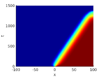
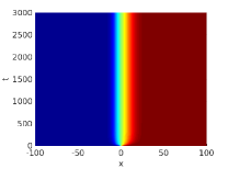
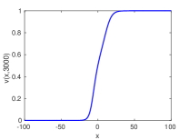
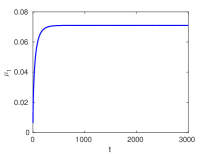
Figure 3.1. QN-front: space-time of $u$ (a), of $v$ (b), profile $v$ (c), velocity $\mu$ (d)

Figure 3.1 shows the time evolution for a travelling front of the QNE for parameters $b_{2}=\tfrac{2}{5}$, $b_{3}=\tfrac{1}{2}$, $b_{4}=\tfrac{17}{20}$, spatial domain $[-100,100]$, initial data $u_{0}(x)=\tfrac{\tanh(x)+1}{2}$ and time range $[0,1500]$. At time $t\approx 1300$ the front leaves the computational domain. Figures 3.1 and 3.1 show the time evolution of the front profile and the velocity obtained by solving the freezing system (2.8) with homogeneous Neumann boundary conditions, $f$ from (3.1), parameters $b_{j}$ and spatial domain as before, initial data $v_{0}=u_{0}$, and the template $\hat{v}=u_{0}$ on the time range $[0,3000]$. The front quickly stabilises at the shape $v_{\star}$ shown in Figure 3.1, and the velocity quickly reaches its asymptotic value $\mu_{\star}\approx 0.07$ as shown in 3.1. For the numerical solution of (1.11) resp. (2.8) we used a FEM space discretisation with Lagrange $C^{0}$-elements and maximal element size $\triangle x=0.3$, the BDF method for time discretisation with maximum order $2$, time step-size $\triangle t=0.3$, relative tolerances $10^{-2}$ and $10^{-3}$, and absolute tolerances $10^{-3}$ and $10^{-4}$, combined with Newton’s method for non-linear equations.

The next example is a two-dimensional system of type (1.12) obtained by writing a scalar complex equation as a real system.

Example 3.2 (Quintic-cubic Ginzburg-Landau equation).

Consider the PDE

$$z_{t}=\alpha\triangle z+g(z),\;z=z(x,t)\in\mathbb{C},\;g(z)=(\delta+\beta|z|^{2}+\gamma|z|^{4})z,\;\alpha,\beta,\gamma\in\mathbb{C},\;\delta\in\mathbb{R},$$

known as the quintic-cubic Ginzburg-Landau equation (short: QCGL).

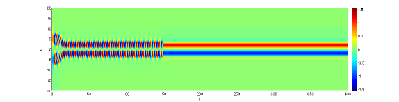
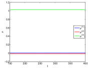
Figure 3.2. Spinning soliton of QCGL: space-time along $x_{2}=0$ (a), velocities (b)

Figure 3.2 shows the time evolution for the real part of a spinning soliton (cross-section at $x_{2}=0$) of the QCGL for parameters $\alpha=\tfrac{1}{2}+\tfrac{1}{2}i$, $\beta=\tfrac{5}{2}+i$, $\gamma=-1-\tfrac{1}{10}i$, $\delta=-\tfrac{1}{2}$, spatial domain $B_{20}(0)=\{x\in\mathbb{R}^{2}:|x|\leqslant 20\}$, initial data $u_{0}(x)=(\mathrm{Re}z_{0},\mathrm{Im}z_{0})^{\top}$ for $z_{0}(x)=\tfrac{x}{5}\exp\left(-\frac{1}{49}|x|^{2}\right)$ and time range $[0,150]$. At time $t=150$ we take the solution data and switch on the freezing system (2.9). Figures 3.2 and 3.2 show the time evolution of the real part of the soliton profile and the velocities obtained by solving (2.9) with homogeneous Neumann boundary conditions, parameters $\alpha,\beta,\gamma,\delta$ and spatial domain as before, initial data $v_{0}=u(\cdot,150)$, template function $\hat{v}=u(\cdot,150)$ and time range $[150,400]$. Approximations of the real part of the soliton profile $v_{\star}$ and the velocities $\mu_{\star}=\left(\begin{smallmatrix}S_{\star}&a_{\star}\\ 0&0\end{smallmatrix}\right)$ with $S_{\star}\approx\left(\begin{smallmatrix}0&1.027\\ -1.027&0\end{smallmatrix}\right)$ and $c_{\star}\approx\left(\begin{smallmatrix}0.003\\ -0.017\end{smallmatrix}\right)$, are shown in Figures 3.3 and 3.2. For the numerical solution of (1.12) resp. (2.9) we used FEM for space discretisation with Lagrange $C^{0}$-elements and maximal element size $\triangle x=0.25$, the BDF method for time discretisation with maximum order $2$, time step-size $\triangle t=0.1$ resp. $\triangle t=0.2$ , relative tolerance $10^{-4}$ resp. $10^{-2}$, and absolute tolerance $10^{-5}$ resp. $10^{-7}$, and Newton’s method for non-linear systems.

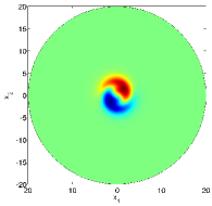
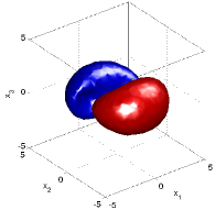
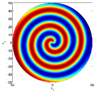
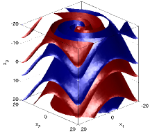
Figure 3.3. Rotating waves: spinning soliton for $d=2$ (a) and $d=3$ (b), spiral wave for $d=2$ (c), untwisted scroll wave for $d=3$ (d)

The spinning solitons of the QCGL from Example 3.2 are a special kind of a localised rotating wave for $d=2$, see Fig. 3.3. Their extension to $d=3$ dimensions is displayed in Fig. 3.3, and non-localised rotating waves, such as spiral waves are shown in Fig. 3.3. Finally, we show a so-called scroll wave in Fig. 3.3. These types of waves occur in various applications, e.g. in the QCGL [20, 42], the $\lambda-\omega$-system [39], the Barkley model [2], and the FitzHugh-Nagumo system [27]. Their treatment via the freezing method is discussed in the papers [43, 10, 6].

3.2. Hyperbolic Systems

The following hyperbolic system in one space dimension may be viewed as a special case of (1.11) with $A=0$,

(3.2) $$u_{t}=Eu_{x}+f(u), u(\cdot,0)=u_{0}.$$

For (3.2) to be well-posed, we assume $E\in\mathbb{R}^{m,m}$ to be real diagonalisable and $f:\mathbb{R}^{m}\rightarrow\mathbb{R}^{m}$ to be sufficiently smooth. As in Section 1.3 travelling waves of (3.2) are solutions of the form (1.13), the underlying Lie group $(G,\circ)$ is the additive group $(\mathbb{R},+)$ acting on functions via translations. The freezing system (2.8) for pursuing profiles and velocities now reads for the unknown quantities $(v,\mu,\gamma)$ as follows,

$$v_{t}= Ev_{\xi}+\mu v_{\xi}+f(v),\quad\quad v(\cdot,0)=v_{0},$$

$$0= \langle\hat{v}_{\xi},v-\hat{v}\rangle_{L^{2}(\mathbb{R},\mathbb{R}^{m})},$$

$$\gamma_{t}= \mu,\quad\quad\gamma(0)=0.$$

The main difference to the parabolic case (2.8) is due to the fact that the unknown function $\mu(t)$ of this PDAE now appears in the principal part of the spatial operator. This creates serious difficulties, both for the numerical and the theoretical analysis. These have been successfully treated in the works [47, 48], and a series of numerical examples appears in [47, 48, 10]. Moreover, with a slightly generalised notion of equivariance (see [53, 47]) the freezing approach has found interesting applications to detecting similarity solutions in Burgers’ equation, see [53, 10] for the one-dimensional and [51, 52] for the multi-dimensional case.

Finally, we refer to the papers [49, 50] in which the stability of travelling waves and the freezing approach is analysed for mixed parabolic-hyperbolic systems of the partitioned form

(3.3) $$u_{t}=\begin{pmatrix}A_{11}&0\\ 0&0\end{pmatrix}u_{xx}+\begin{pmatrix}g(u)\\ B_{22}u_{2}\end{pmatrix}_{x}+\begin{pmatrix}f_{1}(u)\\ f_{2}(u)\end{pmatrix}, u(\cdot,0)=u_{0},$$

with a positive diagonalisable matrix $A_{11}$ and a real diagonalisable matrix $B_{22}$. This covers the famous Hodgkin-Huxley model for propagation of pulses in nerve axons, cf. [10, Ch.3.1].

3.3. Non-Linear Wave Equations

Another area of application are systems of non-linear wave equations in one space dimension

(3.4) $$Mu_{tt}=Au_{xx}+\tilde{f}(u,u_{x},u_{t}), u(\cdot,0)=u_{0},\quad u_{t}(\cdot,0)=v_{0},$$

where $M\in\mathbb{R}^{m,m}$ is invertible, $A\in\mathbb{R}^{m,m}$, $\tilde{f}:\mathbb{R}^{3m}\rightarrow\mathbb{R}^{m}$ is smooth and $u_{0},v_{0}:\mathbb{R}\rightarrow\mathbb{R}^{m}$ denote the initial data. Further we assume $M^{-1}A$ to be positive diagonalisable which implies local well-posedness of (3.4). In case $m=1$, travelling waves (1.13) for equation (3.4) and their global stability have been treated in [30, 29]. The freezing ansatz (2.7) now requires to solve the following second order PDAE (cf. [11, 12])

(3.5) $$Mv_{tt}= (A-\mu_{1}^{2}M)v_{\xi\xi}+2\mu_{1}Mv_{\xi t}+\mu_{2}Mv_{\xi}+\tilde{f}(v,v_{\xi},v_{t}-\mu_{1}v_{\xi})$$

$$0= \langle\hat{v}_{\xi},v-\hat{v}\rangle_{L^{2}(\mathbb{R},\mathbb{R}^{m})},$$

$$\mu_{1,t}= \mu_{2},\quad\gamma_{t}=\mu_{1},$$

$$v(\cdot,0)= u_{0},\quad v_{t}(\cdot,0)=v_{0}+\mu_{1}^{0}u_{0,\xi},\quad\mu_{1}(0)=\mu_{1}^{0},\quad\gamma(0)=0$$

for the unknown quantities $(v,\mu_{1},\mu_{2},\gamma)$. Travelling waves $(v_{\star},\mu_{\star})$ appear as steady states of (3.5) (with $\mu_{1}=\mu_{\star}$, $\mu_{2}=0$) and satisfy the equation

$$0=(A-\mu_{\star}^{2}M)v_{\star,\xi\xi}+f(v_{\star},v_{\star,\xi},-\mu_{\star}v_{\star,\xi}).$$

Differentiating the algebraic constraint in (3.5) w.r.t. time at $t=0$ and inserting the initial conditions leads to a first consistency condition for $\mu_{1}^{0}$

(3.6) $$\mu_{1}^{0}\langle u_{0,\xi},\hat{v}_{\xi}\rangle_{L^{2}}+\langle v_{0},\hat{v}_{\xi}\rangle_{L^{2}}=0,$$

and differentiating twice at $t=0$ gives a consistency condition for $\mu_{2}(0)=\mu_{2}^{0}$:

(3.7) $$0=\langle(M^{-1}A+(\mu_{1}^{0})^{2}I_{m})u_{0,\xi\xi}+2\mu_{1}^{0}v_{0,\xi}+M^{-1}f(u_{0},u_{0,\xi},v_{0}),\hat{v}_{\xi}\rangle_{L^{2}}+\mu_{2}^{0}\langle u_{0,\xi},\hat{v}_{\xi}\rangle_{L^{2}}.$$

The local stability of the PDAE system (3.5) is analysed in [11] while a generalisation to several space dimensions and a numerical example appear in [12]. It is interesting to note that the system (3.4) may be written as a first order system (3.2) of dimension $3m$. Taking a positive square root $N=(M^{-1}A)^{1/2}$ and introducing the variables $U_{1}=u$, $U_{2}=u_{t}+Nu_{x}$, $U_{3}=u_{t}-Nu_{x}+cu$ ($c\in\mathbb{R}$ arbitrary) leads to a system (3.2) with

(3.8) $$E= \begin{pmatrix}N&0&0\\ 0&N&0\\ 0&0&-N\end{pmatrix},\quad f(U)=\begin{pmatrix}-cU_{1}+U_{3}\\ g(U)\\ g(U)+cU_{2}\end{pmatrix}$$

$$g(U)= M^{-1}\tilde{f}(U_{1},\frac{1}{2}N^{-1}(U_{2}-U_{3}+cU_{1}),\frac{1}{2}(U_{2}+U_{3}-cU_{1})).$$

Though we prefer to solve numerically the second order system (3.5), the first order system (with a suitable choice of the constant $c$) is useful for applying the stability results from [48], see [11] and Section 4.

Example 3.3 (Quintic Nagumo wave equation).

Taking the quintic non-linearity $f=\tilde{f}$ from (3.1) with the wave equation (3.4) we obtain the quintic Nagumo wave equation (short: QNWE), see [12].

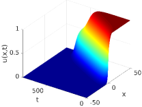
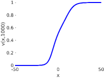
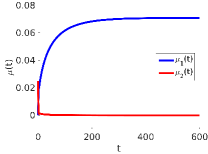
Figure 3.4. QNWE-front: space-time of $u$ (a), $v$ (b), profile $v$ (c), velocity $\mu$ (d)

Figure 3.4 shows the time evolution for a travelling front of the QNWE for parameters $M=\tfrac{1}{2}$, $b_{2}=\tfrac{2}{5}$, $b_{3}=\tfrac{1}{2}$, $b_{4}=\tfrac{17}{20}$, spatial domain $[-50,50]$, initial data $u_{0}(x)=\tfrac{1}{2}(1+\tanh(\tfrac{x}{2}))$, $v_{0}(x)=0$ and time range $[0,800]$. At time $t\approx 600$ the front leaves our computational domain. Figures 3.4 and 3.4 show the time evolution of the front profile and the velocity obtained by solving (3.5) with homogeneous Neumann boundary conditions, parameters $M$, $b_{j}$, spatial domain and initial data as before, template $\hat{v}=u_{0}$ and time range $[0,1000]$. An approximation of the front profile $v_{\star}$ (with $v_{-}=0$, $v_{+}=1$) and the approach towards the limit velocity $\mu_{\star}\approx 0.07$ are shown in Figures 3.4 and 3.4. The data for the numerical solution of (3.4) resp. (3.5) are the same as in Example 3.1, except for the step-sizes $\triangle x=0.1$ and $\triangle t=0.2$.

3.4. Hamiltonian PDEs

So far we mainly considered waves in dissipative PDEs which are detected during simulation via the freezing method due to their asymptotic stability. This changes fundamentally for PDEs with Hamiltonian structure which typically allow several or even infinitely many conserved quantities. They fit into the general class of evolution problems described in Section 1.1 but require quite different techniques for establishing existence and uniqueness of wave solutions [24] as well as their stability ([31, 32]).

As a model example consider the cubic non-linear Schrödinger equation (NLS, see the references [17, 24, 37, 58])

(3.9) $$iu_{t}=-u_{xx}-|u|^{2}u,\quad u(\cdot,0)=u_{0},$$

which may be subsumed under (1.1) with $X=H^{1}(\mathbb{R};\mathbb{C})$ , $Z=H^{3}(\mathbb{R};\mathbb{C})$. Equivariance holds with respect to the action

$$a(\gamma)v=e^{-i\gamma_{1}}v(\cdot-\gamma_{2}),\quad\gamma=(\gamma_{1},\gamma_{2})\in G$$

of the two-dimensional Lie group $G=S^{1}\times\mathbb{R}$. With $\mu=(\mu_{1},\mu_{2})\in\mathbb{R}^{2}$ the freezing system (2.2) is given by

(3.10) $$iv_{t}=-v_{\xi\xi}-|v|^{2}v-\mu_{1}v+i\mu_{2}v_{\xi},\quad v(\cdot,0)=u_{0},$$

and the fixed phase condition (2.5) with some $\hat{v}\in X$ reads

(3.11) $$0=\big{\langle}i\hat{v},v\big{\rangle}_{0}=\big{\langle}\hat{v}_{\xi},v\big{\rangle}_{0},$$

where $\langle u,v\rangle_{0}=\mathrm{Re}\int_{\mathbb{R}}\bar{u}(x)v(x)dx$. There is a well-known two-parameter family of solitary wave solutions given by

(3.12) $$u_{\star}(x,t)= e^{i\mu_{1}t}v_{\star}(x-\mu_{2}t;\mu_{1},\mu_{2}),$$

$$v_{\star}(\xi;\mu_{1},\mu_{2})= \frac{\omega\sqrt{2}e^{i\mu_{2}\xi/2}}{\mathrm{cosh}(\omega\xi)},\quad\omega^{2}=\mu_{1}-\frac{\mu_{2}^{2}}{4},$$

see for example [23, Ch.II.3]. For the following numerical computations we choose parameter values $\mu_{2}=0.3$, $\omega=1$.

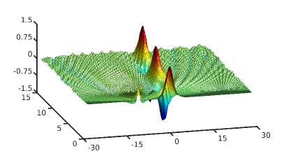
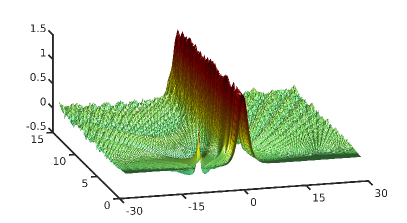
Figure 3.5. Solitary wave of the NLS with spike-like initial perturbation:
direct numerical simulation (left) vs. solution of the freezing system (right)

Discretisation in time is done via a split-step Fourier method with step size $\Delta t=10^{-3}$. The spatial grid is formed by $2K=256$ equidistant points on the interval $[x_{-},x_{+}]$ with $x_{+}=-x_{-}=\tfrac{\pi}{0.11}\approx 28.56$. A spike-like perturbation at $x=-11$ is added to the initial data. Figure 3.5 shows the solution for both the original system and the freezing system. Clearly, the freezing system prevents the wave from rotating and travelling, while the interference patterns caused by the initial perturbation are essentially preserved. A theoretical result supporting these observations will be described in Section 4.4, and a detailed presentation can be found in the thesis [21].

3.5. Multi-Waves

For a numerical experiment of decomposing and freezing multi-waves we take up Example 3.1 of the Quintic Nagumo equation (QNE).

Example 3.4 (Quintic Nagumo equation).

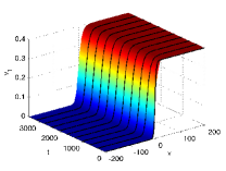
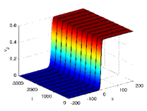
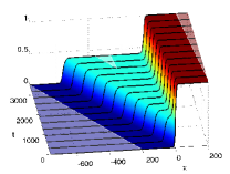
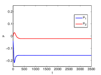
Figure 3.6. $2$-front of QNE: profile $v_{1}$ (a), profile $v_{2}$ (b), superposition (c), and velocities $\mu_{1},\mu_{2}$ (d)

Figure 3.6 shows the time evolution of the superposition $\sum_{j=1}^{2}v_{j}(x-\gamma_{j}(t),t)$, which can be considered as an approximation of a travelling $2$-front $u$ of the original QNE (2.10) with $f$ from (3.1). The quantities $(v_{j},\mu_{j})$ are the solutions of (2.12) and provides us approximations of $(v_{\star,j},\mu_{\star,j})$. Figure 3.6 shows that the lower front $v_{1}$ (travelling at speed $\mu_{1}$) is faster than the upper front $v_{2}$ (travelling at speed $\mu_{2}$), i.e. we may expect $\mu_{\star,1}<\mu_{\star,2}<0$. Figure 3.6 and 3.6 (resp. 3.6) show the time evolution of the single front profiles $v_{1}$ and $v_{2}$ (resp. the velocities $\mu_{1},\mu_{2}$) obtained by solving (2.12) with homogeneous Neumann boundary conditions, $f$ from (3.1), parameters $b_{2}=\tfrac{1}{32}$, $b_{3}=\tfrac{2}{5}$, $b_{4}=\tfrac{73}{100}$, spatial domain $[-200,200]$, multi-waves $N=2$, initial data $v_{1}^{0}(\xi)=\tfrac{v_{2}^{-}}{2}\left(\tanh(\tfrac{\xi}{5})+1\right)$, $v_{2}^{0}(\xi)=\tfrac{1-v_{2}^{-}}{2}\left(\tanh(\tfrac{\xi}{5})+1\right)$ with $v_{2}^{-}=b_{3}$, $\gamma_{1}^{0}=\gamma_{2}^{0}=0$, templates $\hat{v}_{j}=v_{j}^{0}$, bump function $\varphi(\xi)=\mathrm{sech}(\tfrac{\xi}{20})$ and time range $[0,3000]$. Approximations of the single front profiles $v_{\star,j}$ (with $v_{1}^{-}=0$, $v_{1}^{+}=a_{4}=v_{2}^{-}$, $v_{2}^{+}=1$) and velocities $\mu_{\star,1}\approx-0.159$, $\mu_{\star,1}\approx-0.021$ are shown in Figure 3.6, 3.6 and 3.6. For the numerical solution of (2.12) we used the FEM for space discretisation with Lagrange $C^{0}$-elements and maximal element size $\triangle x=0.4$, the BDF method for time discretisation with maximum order $2$, intermediate time steps, time step-size $\triangle t=0.8$, and the Newton method for solving non-linear equations.

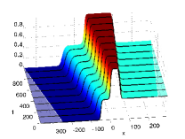
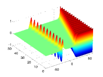
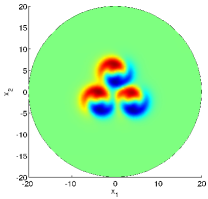
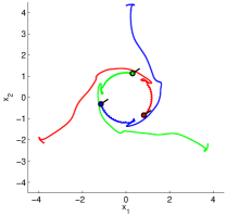
Figure 3.7. Multiwaves: $3$-front of QNE (a), Pulse-Front of QCGL (b), $3$-soliton of QCGL (c) and position of centres (d)

Travelling $2$-fronts as in Example 3.4 are a special class of multi-waves. The decompose and freeze method (short: DFM) easily extends to larger numbers of fronts, e.g. $3$-fronts (see Fig. 3.7), and can be used to analyse wave interaction processes, for example repulsion and collision of waves. Moreover, the DFM extends to general multi-structures, e.g. to a superposition of a phase-rotating pulse and a travelling phase-rotating front (see Fig. 3.7), and to higher space dimensions, see the three spinning multi-solitons in Fig. 3.7) with the interactions represented by the traces of their centres in Fig. 3.7. For the DFM we refer to the works [10, 57, 13]. Extensions of the DFM to rotating multi-solitons including numerical experiments can be found in [10, 43].

4. Stability of Relative Equilibria

The issue of stability is fundamental to all wave phenomena considered here. Since relative equilibria come in families due to the group action (see Section 1.2) the classical notions of (Lyapunov)-stability and asymptotic (Lyapunov)-stability are replaced by the notions of orbital stability and stability with asymptotic phase.

4.1. Notions of stability and the co-moving frame equation

In order to have some flexibility for the application to PDEs, the following definition uses two norms $\|\cdot\|_{1}$ and $\|\cdot\|_{2}$ which need not agree with the norms in the Banach spaces $Z$ and $X$. Moreover, depending on the type of PDE, a solution concept different from the strong solution in Definition 1.2 may be necessary.

Definition 4.1.

A relative equilibrium $(v_{\star},\gamma_{\star})$ of (1.4) is called orbitally stable with respect to norms $\|\cdot\|_{1}$ and $\|\cdot\|_{2}$ if for any $\varepsilon>0$ there exists $\delta>0$ such that the Cauchy problem (1.4) has a unique strong solution $u$ for $u_{0}\in Z$ with $\|u_{0}-v_{\star}\|_{1}\leq\delta$, and the solution satisfies

$$\mathrm{inf}_{\gamma\in G}\|u(t)-a(\gamma)v_{\star}\|_{2}\leq\varepsilon\quad\forall t\geq 0.$$

It is called stable with asymptotic phase if for any $\varepsilon>0$ there exists $\delta>0$ such that for all initial values $u_{0}\in Z$ with $\|u_{0}-v_{\star}\|_{1}\leq\delta$ the Cauchy problem (1.4) has a unique strong solution $u$, and for some $\gamma_{\infty}=\gamma_{\infty}(u_{0})\in G$ the solution satisfies

$$\|u(t)-a(\gamma_{\infty}\circ\gamma_{\star}(t))v_{\star}\|_{2}\begin{cases}\leq\varepsilon\quad\forall t\geq 0,\\ \rightarrow 0\quad\text{as}\quad t\rightarrow\infty.\end{cases}$$

Stability in general requires to investigate the solution of (1.4) for initial data $u_{0}=u_{\star}+v_{0}$ which are small perturbations of the wave profile. For this we transform into a co-moving frame via

$$u(t)=a(\gamma_{\star}(t))v(t),\quad t\geq 0,$$

which by contrast to the general ansatz (2.1) assumes the group orbit $\gamma_{\star}$ to be known. Instead of (2.2) one obtains the co-moving frame equation

(4.1) $$v_{t}(t)=F(v(t))-d_{\gamma}[a(\mathbbm{1})v(t)]\mu_{\star},\quad v(0)=v_{\star}+v_{0}.$$

Linearising about $v_{\star}$ in a formal sense leads to consider the linear operator

(4.2) $$\mathcal{L}w=DF(v_{\star})w-d_{\gamma}[a(\mathbbm{1})w]\mu_{\star},\quad w\in Z.$$

If the topology on $Z$ is strong enough, then $DF$ is in fact the Fréchet derivative of $F$, and this point of view is sufficient for our applications to semi-linear PDEs in Section 3. The general procedure then is to deduce non-linear stability in the sense of Definition 4.1 from spectral properties of the operator $\mathcal{L}$. One says that the principle of linearised stability holds if such a conclusion is valid. A minimal requirement is that the spectrum lies in the left half-plane, i.e.

$$\sigma(\mathcal{L})\subseteq\mathbb{C}_{-}=\{\lambda\in\mathbb{C}:\mathrm{Re}(\lambda)\leq 0\}.$$

However the special properties of the PDEs considered here usually require more:

1. determine eigenvalues on the imaginary axis caused by the group action,

2. analyse the essential spectrum $\sigma_{\mathrm{ess}}(\mathcal{L})\subseteq\sigma(\mathcal{L})$ which arises from the loss of compactness for differential operators on unbounded domains,

3. compute isolated eigenvalues of the point spectrum $\sigma_{\mathrm{pt}}(\mathcal{L})\subseteq\sigma(\mathcal{L})$ different from those in (P1), either by a theoretical or by a numerical tool.

Let us finally note that a proof of non-linear stability becomes particularly delicate if there is no spectral gap between the eigenvalues from (P1) and the remaining spectrum. This occurs if the spectrum touches the imaginary axis (wave trains, spiral waves, see [22], [56]) or lies on the imaginary axis (Hamiltonian case).

4.2. Spectral Structures

Hardly anything can be said about problems (P2), (P3) above within the abstract framework of equations (1.4),(4.1). However, the eigenvalues caused by symmetry have some general structure. For this purpose recall the Lie bracket $[\cdot,\cdot]:\mathfrak{g}\times\mathfrak{g}\rightarrow\mathfrak{g}$ (see e.g. [28, Ch.8]) which turns $\mathfrak{g}=T_{\mathbbm{1}}G$ into a Lie algebra. The abstract definition of the bracket is in terms of the adjoint representation $\mathrm{Ad}(g):\mathfrak{g}\rightarrow\mathfrak{g}$ of $g\in G$ given by

$$\mathrm{Ad}(g)\nu= d_{h}[g\circ h\circ g^{-1}]_{|h=\mathbbm{1}}\nu,\quad\nu\in\mathfrak{g},$$

$$[\mu,\nu]= d_{g}[\mathrm{Ad}(g)\nu]_{|g=\mathbbm{1}}(\mu),\quad\mu,\nu\in\mathfrak{g}.$$

It is reasonable to look for eigenfunctions of $\mathcal{L}$ of the type $w=d_{\gamma}[a(\mathbbm{1})v_{\star}]\mu,\mu\in\mathfrak{g}_{\mathbb{C}}$, where $\mathfrak{g}_{\mathbb{C}}$ denotes the complexified Lie algebra and $d_{\gamma}[a(\mathbbm{1})v_{\star}]$ denotes the complexified operator.

Theorem 4.2.

Let $v_{\star}\in Z$,$\gamma_{\star}(t)=\exp(t\mu_{\star}),t\geq 0$ be a relative equilibrium of (1.1) such that $d_{\gamma}[a(\mathbbm{1})v_{\star}]$ maps $\mathfrak{g}$ into $Z$. Then $w=d_{\gamma}[a(\mathbbm{1})v_{\star}]\mu,\mu\in\mathfrak{g}_{\mathbb{C}}$ solves the (complexified) eigenvalue problem

(4.3) $$(\lambda I-\mathcal{L})w=0$$

if and only if $\mu$ satisfies

$$d_{\gamma}[a(\mathbbm{1})v_{\star}](\lambda\mu-[\mu,\mu_{\star}])=0.$$

In particular, if the stabiliser $H(v_{\star})$ is trivial (see (1.9)), then independent eigenvectors $\mu_{j},j=1,\ldots,k$ of $[\cdot,\mu_{\star}]:\mathfrak{g}\rightarrow\mathfrak{g}$ lead to independent eigenfunctions $w_{j}=d_{\gamma}[a(\mathbbm{1})v_{\star}]\mu_{j},j=1,\ldots,k$ of (4.3).

Proof.

For the family of relative equilibria (1.10) we have by the chain rule

$$F(a(\gamma(g,t))a(g)v_{\star})= \frac{d}{dt}\left[a(\gamma(g,t))(a(g)v_{\star})\right]$$

$$= d_{\gamma}\left[a(g\circ\gamma_{\star}(t)\circ g^{-1})(a(g)v_{\star})\right]d_{h}(g\circ h\circ g^{-1})_{|h=\gamma_{\star}(t)}\gamma^{\prime}_{\star}(t),$$

which upon evaluation at $t=0$ yields

$$F(a(g)v_{\star})= d_{\gamma}\left[a(\mathbbm{1})(a(g)v_{\star})\right]\mathrm{Ad}(g)\mu_{\star}.$$

We differentiate with respect to $g\in G$ and apply this to $\mu\in T_{g}G$:

$$DF(a(g)v_{\star})d_{\gamma}[a(g)v_{\star}]\mu= d_{\gamma}[a(\mathbbm{1})(d_{\gamma}[a(g)v_{\star}]\mu)]\mathrm{Ad}(g)\mu_{\star}$$

$$+ d_{\gamma}[a(\mathbbm{1})(a(g)v_{\star})]d_{g}[\mathrm{Ad}(g)\mu_{\star}]\mu,$$

which upon evaluation at $g=\mathbbm{1},\mu\in\mathfrak{g}$ gives

$$DF(v_{\star})d_{\gamma}[a(\mathbbm{1})v_{\star}]\mu= d_{\gamma}[a(\mathbbm{1})(d_{\gamma}[a(\mathbbm{1})v_{\star}]\mu)]\mu_{\star}+d_{\gamma}[a(\mathbbm{1})v_{\star}][\mu,\mu_{\star}].$$

Therefore, the eigenvalue problem (4.3) with $w=d_{\gamma}[a(\mathbbm{1})v_{\star}]\mu$ is equivalent to

$$0= \lambda w-DF(v_{\star})w+d_{\gamma}[a(\mathbbm{1})w]\mu_{\star}$$

$$= \lambda d_{\gamma}[a(\mathbbm{1})v_{\star}]\mu-DF(v_{\star})d_{\gamma}[a(\mathbbm{1})v_{\star}]\mu+d_{\gamma}[a(\mathbbm{1})(d_{\gamma}[a(\mathbbm{1})v_{\star}]\mu)]\mu_{\star}$$

$$= d_{\gamma}[a(\mathbbm{1})v_{\star}](\lambda\mu-[\mu,\mu_{\star}]),$$

which proves our assertion. ∎

Theorem 4.2 shows that the geometric multiplicity of the eigenvalue $\lambda=0$ is at least the dimension of the centraliser of $\mu_{\star}$ given by

$$\mathfrak{g}_{0}(\mu_{\star}):=\{\mu\in\mathfrak{g}:[\mu,\mu_{\star}]=0\}.$$

If the group $G$ is represented as a subgroup of the matrix group $\mathrm{GL}(\mathbb{R}^{N})$ for some $N\in\mathbb{N}$ then the Lie bracket agrees with the commutator. It is not difficult to see that the spectrum of the linear map $\mu\mapsto[\mu,\mu_{\star}]$ always satisfies

(4.4) $$\sigma([\cdot,\mu_{\star}])\subseteq\{\lambda_{1}-\lambda_{2}:\lambda_{1},\lambda_{2}\in\sigma(\mu_{\star})\}=\sigma(\mu_{\star})-\sigma(\mu_{\star}).$$

The special elements $\mu_{\star}=\left(\begin{smallmatrix}S_{\star}&c_{\star}\\ 0&0\end{smallmatrix}\right)$ from $\mathfrak{se}(d)$ (see (1.15)) occur with rotating waves (1.16) and satisfy $\sigma(\mu_{\star})\subseteq i\mathbb{R}$ as well as $\sigma(\mu_{\star})=-\sigma(\mu_{\star})$. Let $\mu_{1},\ldots,\mu_{d}$ be the eigenvalues of the skew-symmetric matrix $S_{\star}$, then one finds

(4.5) $$\sigma([\cdot,\mu_{\star}])=\{\mu\in\mathbb{C}:\mu\in\sigma(S_{\star})\;\text{or}\;\mu=\mu_{j}+\mu_{k}\;\text{for some}\;j<k\},$$

see [16],[8] for the computation of eigenvalues and corresponding eigenvectors.

4.3. Stability with Asymptotic Phase

We discuss sufficient conditions for the stability with asymptotic phase in case of our two model equations (1.11),(1.12) (see [10],[35],[36],[55],[60]).

For a travelling wave $(v_{\star},\mu_{\star})$ the linearised operator $\mathcal{L}$ from (4.2) reads

(4.6) $$\mathcal{L}w= Aw_{\xi\xi}+(\mu_{\star}I_{m}+D_{2}f(v_{\star},v_{\star,\xi}))w_{\xi}+D_{1}f(v_{\star},v_{\star,\xi})w$$

$$= Aw_{\xi\xi}+B(\cdot)w_{\xi}+C(\cdot)w.$$

We consider the case of a front

(4.7) $$\lim_{\xi\rightarrow\pm\infty}v_{\star}(\xi)=v_{\pm},\quad\lim_{\xi\rightarrow\pm\infty}v_{\star,\xi}(\xi)=0,$$

which is covered by our abstract approach only in case $v_{\pm}=0$, see Remark 1.1. Note, however, that $\mathcal{L}:H^{2}(\mathbb{R},\mathbb{R}^{m})\to L^{2}(\mathbb{R},\mathbb{R}^{m})$ is well defined in the general case (4.7), and that it has the eigenvalue $0$ with eigenfunction $w=v_{\star,\xi}$, cf. Theorem 4.2 and (4.4) with $0\in\sigma(\mu_{\star})$. The essential spectrum of $\mathcal{L}$ is determined by the constant coefficient operators

(4.8) $$\mathcal{L}^{\pm}=A\partial_{\xi}^{2}+B_{\pm}\partial_{\xi}+C_{\pm},\quad C_{\pm}=D_{1}f(v_{\pm},0),\quad B_{\pm}=\mu_{\star}I_{m}+D_{2}f(v_{\pm},0).$$

Bounded solutions of $(\lambda I-\mathcal{L}^{\pm})w=0$ are of the form $w(\xi)=e^{i\omega\xi},\omega\in\mathbb{R}$ which leads to the definition of the dispersion set

(4.9) $$\sigma_{\mathrm{disp}}(\mathcal{L})=\left\{\lambda\in\mathbb{C}:\lambda\in\sigma(-\omega^{2}A+i\omega B_{\pm}+C_{\pm})\;\text{for some sign}\;\pm\;\text{and}\;\omega\in\mathbb{R}\right\}.$$

By Weyl’s theorem on invariance of the essential spectrum under relatively compact perturbations (see [35],[36]) one finds $\sigma_{\mathrm{disp}}(\mathcal{L})\subseteq\sigma_{\mathrm{ess}}(\mathcal{L})$ and, moreover, that the connected component $U$ of $\mathbb{C}\setminus\sigma_{\mathrm{disp}}(\mathcal{L})$ containing a positive real semi-axis satisfies $U\subseteq(\rho(\mathcal{L})\cup\sigma_{\mathrm{pt}}(\mathcal{L}))$. Therefore, the issues (P2) and (P3) from Section 4.1 are resolved by requiring for some $\beta>0$ the following spectral conditions

(4.10) $$\mathrm{Re}\,\sigma_{\mathrm{disp}}(\mathcal{L})\leq-\beta<0,$$

(4.11) $$\mathrm{Re}\left(\sigma_{\mathrm{pt}}(\mathcal{L})\setminus\{0\}\right)\leq-\beta<0\quad\text{and the eigenvalue}\;0\;\text{is simple}.$$

A common analytical tool to verify assumption (4.11) in applications is to study the zeroes of the so-called Evans function, see [36],[55]. For numerical purposes however, we prefer to solve boundary eigenvalue problems subject to finite boundary conditions and to employ a contour method, see Section 5 and [5].

Theorem 4.3.

Let the spectral assumptions (4.10),(4.11) above hold and let $f$ be of the form

(4.12) $$f(u,v)=f_{1}(u)+f_{2}(u)v,\quad f_{1}\in C^{2}(\mathbb{R}^{m},\mathbb{R}^{m}),f_{2}\in C^{2}(\mathbb{R}^{m},\mathbb{R}^{m,m}).$$

Then a travelling wave $(v_{\star},\mu_{\star})$ of (1.11) is stable with asymptotic phase for solutions in the regularity class $v_{\star}+\left(C([0,\infty),H^{1}(\mathbb{R},\mathbb{R}^{m}))\cap C^{1}([0,\infty),L^{2}(\mathbb{R},\mathbb{R}^{m}))\right)$ and with respect to the norm $\|\cdot\|_{1}=\|\cdot\|_{2}=\|\cdot\|_{H^{1}}$.

Remark 4.4.

The semilinear case $f_{2}\equiv 0$ is well studied, see e.g. [35],[36],[55]. The more general form (4.12) includes Burgers equation ($f_{2}(u)=u$) and is treated in [59], [60]. Note that the global Lipschitz conditions imposed there can be localised via the Sobolev embedding $H^{1}(\mathbb{R},\mathbb{R}^{m})\subset L^{\infty}(\mathbb{R},\mathbb{R}^{m})$.

In Sections 3.2 and 3.3 we referred to stability results for travelling waves in hyperbolic systems of first order (3.2), (3.3) and of second order (3.4). Here we consider in more detail the stability of rotating waves for the model system (1.12). Following [6] we restrict to $d=2$ and $A=I_{m}$. Extensions to $d\geq 3$ are based on [7],[8] and will be indicated below. Moreover, we mention an alternative approach [54] towards asymptotic stability (without asymptotic phase) based on a centre manifold reduction.

As in (1.16) consider a rotating wave $v_{\star}\in H^{2}_{\mathrm{Eucl}}(\mathbb{R}^{2},\mathbb{R}^{m})$ centred at $x_{\star}=0$ and with $S_{\star}=\left(\begin{smallmatrix}0&-\mu_{\star}\\ \mu_{\star}&0\end{smallmatrix}\right),\mu_{\star}\neq 0$. We assume decay of derivatives up to order $2$

$$\sup_{|\xi|\geq R}|D^{\alpha}v_{\star}(\xi)|\to 0\quad\text{as}\;R\to\infty\quad\text{for}\;|\alpha|\leq 2$$

and stability of the linearisation at infinity in the sense of

(4.13) $$\mathrm{Re}\,\langle Df(0)w,w\rangle\leq-\beta|w|^{2}\quad\text{for all}\;w\in\mathbb{C}^{m}\quad\text{and some}\;\beta>0.$$

This assumption guarantees that the essential spectrum of the linear operator $\mathcal{L}:H^{2}_{\mathrm{Eucl}}(\mathbb{R}^{2},\mathbb{R}^{m})\to L^{2}(\mathbb{R}^{2},\mathbb{R}^{m})$ defined by

(4.14) $$\mathcal{L}v=\Delta v+\mathcal{L}_{S_{\star}}v+Df(v_{\star})v,$$

lies in the open left half plane. As for the abstract result (4.5) one finds that $\mathcal{L}$ has eigenvalues $0,\pm i\mu_{\star}$ with corresponding eigenfunctions $\mathcal{L}_{S_{\star}}v_{\star}$ and $D_{1}v_{\star}\pm iD_{2}v_{\star}$. The appropriate assumption on the point spectrum of $\mathcal{L}$ then is to require that for some $\beta>0$ (which agrees w.l.o.g with $\beta$ from (4.13)):

$$\text{The eigenvalues}\ 0,\pm i\mu_{\star}\;\text{are simple and the only ones of}\;\mathcal{L}\;\text{with}\;\mathrm{Re}\geq-\beta.$$

Theorem 4.5.

Let $f\in C^{4}(\mathbb{R}^{m},\mathbb{R}^{m})$ and let the rotating wave $(v_{\star},S_{\star})$ satisfy the spectral assumptions above. Then the rotating wave is asymptotically stable with asymptotic phase for the equation (1.12) with initial data $u_{0}\in H^{2}_{\mathrm{Eucl}}(\mathbb{R}^{2},\mathbb{R}^{m})$, for strong solutions in the function class $C^{1}([0,\infty),L^{2}(\mathbb{R}^{2},\mathbb{R}^{m}))\cap C([0,\infty),H^{2}(\mathbb{R}^{2},\mathbb{R}^{m}))$, and with respect to the norms $\|\cdot\|_{1}=\|\cdot\|_{H^{2}_{\mathrm{Eucl}}}$, $\|\cdot\|_{2}=\|\cdot\|_{H^{2}}$.

Let us comment on the assumptions of this theorem and possible extensions. In [7, Cor.4.3] it is shown that the derivatives $D^{\alpha}v_{\star}$,$1\leq|\alpha|\leq 2$ of the solution decay even exponentially as $R\to\infty$ if (4.13) holds and if $\sup_{|\xi|\geq R}|v_{\star}(\xi)|$ falls below a certain computable threshold. Moreover, according to [8, Theorem 2.8] the operator $\lambda I-\mathcal{L}:H^{2}_{\mathrm{Eucl}}(\mathbb{R}^{2},\mathbb{R}^{m})\to L^{2}(\mathbb{R}^{2},\mathbb{R}^{m})$ is Fredholm of index $0$ for values $\mathrm{Re}(\lambda)>-\beta$. Hence the eigenvalues $0,\pm i\mu_{\star}$ are isolated and of finite multiplicity. These results generalise to arbitrary space dimensions $d\geq 3$ if the non-linearity and the solution $v_{\star}$ are sufficiently smooth. Then it can also be shown that the eigenfunctions which belong to eigenvalues on the imaginary axis and which are induced by symmetry, decay exponentially in space. This suggests that the non-linear stability Theorem 4.5 genereralises to space dimensions $d\geq 3$ , but details have not been worked out yet.

4.4. Lyapunov Stability of the Freezing Method

The numerical experiments in Section 3 confirm for various types of PDEs that the abstract freezing system (2.2),(2.5) has a Lyapunov-stable equilibrium whenever the original equation (1.1) has a relative equilibrium which is stable with asymptotic phase. Moreover, one expects this property to persist under numerical approximations, such as truncation to a bounded domain with suitable boundary conditions as well as discretisations of space and time. In this section we discuss a few instances where corresponding analytical results are available.

The following result for travelling waves is taken from [59, Theorem 1.13].

Theorem 4.6.

Let the assumptions of Theorem 4.3 hold and let the template function $\hat{v}$ in (2.8) satisfy

$$\hat{v}\in v_{\star}+H^{2}(\mathbb{R},\mathbb{R}^{m}),\quad\langle\hat{v}_{\xi},v_{\star}-\hat{v}\rangle_{L^{2}}=0,\quad\langle\hat{v}_{\xi},v_{\star,\xi}\rangle_{L^{2}}\neq 0.$$

Then the travelling wave $(v_{\star},\mu_{\star})$ is asymptotically stable for (2.8). More precisely, there exist constants $\delta,C,\alpha>0$ such that (2.8) has a unique solution $(v,\mu)$ if $\|u_{0}-v_{\star}\|_{H^{1}}\leq\delta$ and $\langle\hat{v}_{\xi},u_{0}-\hat{v}\rangle_{L^{2}}=0$. Existence and uniqueness holds for solutions with regularity $\mu\in C[0,\infty)$, $v\in C([0,\infty),H^{1}(\mathbb{R},\mathbb{R}^{m}))$, $v_{t},f(v,v_{\xi})\in C([0,\infty),L^{2}(\mathbb{R},\mathbb{R}^{m}))$, and $v(t)\in H^{2}(\mathbb{R},\mathbb{R}^{m})$ for $t>0$. Furthermore, the following estimate is valid

$$\|v(t)-v_{\star}\|_{H^{1}}+|\mu(t)-\mu_{\star}|\leq Ce^{-\alpha t}\|u_{0}-v_{\star}\|_{H^{1}},\quad t\geq 0.$$

The papers [60],[61] transfer these properties to a spatially discretised sytem (time is left continuous) on bounded intervals $J=[x_{-},x_{+}]$ with general linear boundary conditions

(4.15) $$P_{-}(v(x_{-})-v_{-})+Q_{-}v_{\xi}(x_{-})+P_{+}(v(x_{+})-v_{+})+Q_{+}v_{\xi}(x_{+})=0,$$

where $P_{\pm},Q_{\pm}\mathbb{R}^{2m,m}$ and $v_{\pm}$ are given by (4.7). An essential condition for stability is [61, Hypothesis 2.5]

(4.16) $$\det\begin{pmatrix}\begin{pmatrix}P_{-}&Q_{-}\end{pmatrix}\begin{pmatrix}Y_{-}^{s}(\lambda)\\ Y_{-}^{s}(\lambda)\Lambda_{-}^{s}(\lambda)\end{pmatrix}&\begin{pmatrix}P_{+}&Q_{+}\end{pmatrix}\begin{pmatrix}Y_{+}^{u}(\lambda)\\ Y_{+}^{u}(\lambda)\Lambda_{+}^{u}(\lambda)\end{pmatrix}\end{pmatrix}\neq 0$$

for all $\lambda\in\mathbb{C}$ satisfying $\mathrm{Re}\lambda\geq-\beta$ and $|\lambda|\leq C$ for some large constant $C$. Here the matrices $Y_{\pm}^{s,u}(\lambda)\in\mathbb{R}^{m,m}$ are invertible and together with $\Lambda_{\pm}^{s,u}(\lambda)\in\mathbb{R}^{m,m}$ solve the quadratic eigenvalue problem (cf. (4.8))

(4.17) $$AY\Lambda^{2}+B_{\pm}Y\Lambda+(C_{\pm}-\lambda I_{m})Y=0$$

such that $\mathrm{Re}\,\sigma(\Lambda_{\pm}^{s}(\lambda))<0<\mathrm{Re}\,\sigma(\Lambda_{\pm}^{u}(\lambda))$. Condition (4.10) on the dispersion set (4.9) ensures that (4.17) has $m$ stable and $m$ unstable eigenvalues. A counterexample in [61, Ch.5.2] shows that violation of (4.16) creates instabilities of the numerical solution even if all conditions of Theorem 4.6 are satisfied.

We proceed with two stability results recently obtained for the freezing formulation of the semilinear wave equation (3.5) and of the NLS (3.9). The assumptions on (3.4) are as follows

$$\tilde{f}\in C^{3}(\mathbb{R}^{3m},\mathbb{R}^{m}),$$

$$M\;\text{is invertible},\quad M^{-1}A\;\text{ is diagonalisable with positive eigenvalues,}$$

$$(v_{\star},\mu_{\star})\in C^{2}_{b}(\mathbb{R},\mathbb{R}^{m})\times\mathbb{R}\;\text{ is a travelling wave of}\;\eqref{b3-e4.3.1}\;\text{with}$$

$$v_{\star,\xi}\in H^{3}(\mathbb{R},\mathbb{R}^{m}),\quad\lim_{\xi\to\pm\infty}(v_{\star},v_{\star,\xi})(\xi)=(v_{\pm},0),\;\tilde{f}(v_{\pm},0,0)=0,$$

$$A-\mu_{\star}^{2}M\;\text{is invertible}.$$

The spectral assumptions concern the quadratic operator polynomial obtained from linearising the comoving frame equation in the first line of (3.5)

(4.18) $$\mathcal{P}(\lambda,\partial_{\xi})= M\lambda^{2}-(D_{3}\tilde{f}(\star)+2\mu_{\star}M\partial_{\xi})\lambda-(A-\mu_{\star}^{2}M)\partial_{\xi}^{2}-D_{1}\tilde{f}(\star)$$

$$+ (\mu_{\star}D_{3}\tilde{f}(\star)-D_{2}\tilde{f}(\star))\partial_{\xi},\quad(\star)=(v_{\star},v_{\star,\xi},-\mu_{\star}v_{\star,\xi}).$$

From this we obtain the matrix polynomials $\mathcal{P}_{\pm}(\lambda,\omega)$ by replacing the argument $(\star)$ by its limit $(v_{\pm},0,0)$ as $\xi\to\pm\infty$ and the operator $\partial_{\xi}$ by its Fourier symbol $i\omega$. Then the dispersion set is defined as follows

$$\sigma_{\mathrm{disp}}(\mathcal{P})=\{\lambda\in\mathbb{C}:\det(\mathcal{P}_{\pm}(\lambda,\omega))=0:\text{for some sign}\;\pm\;\text{and}\;\omega\in\mathbb{R}\}.$$

The conditions analogous to (4.10), (4.11) are then

$$\mathrm{Re}\,\sigma_{\mathrm{disp}}(\mathcal{P})\leq-\beta<0,$$

$$\mathrm{Re}\left(\sigma_{\mathrm{pt}}(\mathcal{P}(\cdot,\partial_{\xi}))\setminus\{0\}\right)\leq-\beta<0,\quad\text{and the eigenvalue}\;0\;\text{is simple}.$$

Theorem 4.7.

Let the assumptions above be satisfied and let the template function $\hat{v}$ in (3.5) fulfil

$$\hat{v}\in v_{\star}+H^{1}(\mathbb{R},\mathbb{R}^{m}),\quad\langle\hat{v}-v_{\star},\hat{v}_{\xi}\rangle_{L^{2}}=0,\quad\langle v_{\star,\xi},\hat{v}_{\xi}\rangle_{L^{2}}\neq 0.$$

Then the pair $(v_{\star},\mu_{\star})$ is asymptotically stable for the PDAE (3.5). More precisely, for all $0<\eta<\beta$ there exist $\rho,C>0$ such that for all $u_{0}\in v_{\star}+H^{3}(\mathbb{R},\mathbb{R}^{m})$, $v_{0}\in H^{2}(\mathbb{R},\mathbb{R}^{m})$, $\mu_{1}^{0}\in\mathbb{R}$ which satisfy

$$\|u_{0}-v_{\star}\|_{H^{3}}+\|v_{0}+\mu_{\star}v_{\star,\xi}\|_{H^{2}}\leq\rho$$

as well as the consistency condition (3.6), the system (3.5) has a unique solution $(v,\mu_{1},\mu_{2})$ with $\mu_{1}\in C^{1}[0,\infty)$, $\mu_{2}\in C[0,\infty)$ and regularity

$$v-v_{\star}\in C^{2}([0,\infty),L^{2}(\mathbb{R},\mathbb{R}^{m}))\cap C^{1}([0,\infty),H^{1}(\mathbb{R},\mathbb{R}^{m}))\cap C([0,\infty),H^{2}(\mathbb{R},\mathbb{R}^{m})).$$

The following estimate holds for the solution

(4.19) $$\|v(\cdot,t)-v_{\star}\|_{H^{2}}+\|v_{t}(\cdot,t)\|_{H^{1}}+|\mu_{1}(t)-\mu_{\star}|\leq Ce^{-\eta t}(\|u_{0}-v_{\star}\|_{H^{3}}+\|v_{0}+\mu_{\star}v_{\star,\xi}\|_{H^{2}}).$$

Note that the second consistency condition (3.7) does not appear in the theorem but is used in the proof to make the acceleration $\mu_{2}$ continuous at $t=0$. The proof of the theorem builds on a careful reduction to the first order system (3.8) and on an application of the stability theorem from [48]. The theory for first order systems is also the reason for measuring the convergence (4.19) in a weaker norm than the initial values.

Finally, we state a recent result on the Lyapunov-stability of the freezing method for the non-linear Schrödinger equation (3.10),(3.11). It is a very special case of a general stability result from the thesis [21, Ch.2] which applies to Hamiltonian PDEs that are equivariant w.r.t. the action of a Lie group. The assumptions are taken from the abstract framework of [32] which is a seminal paper on the stability of solitary waves.

The following theorem is concerned with the waves (3.12) for fixed values $\mu_{\star,1},\mu_{\star,2}$ satisfying $4\mu_{\star,1}>\mu_{\star,2}^{2}$.

Theorem 4.8.

Let $\hat{v}\in H^{3}(\mathbb{R},\mathbb{C})$ be a template function such that

$$\langle i\hat{v},v_{\star}\rangle_{0}=0,\quad\langle\hat{v}_{x},v_{\star}\rangle_{0}=0,$$

$$\begin{pmatrix}\langle i\hat{v},iv_{\star}\rangle_{0}&\langle i\hat{v},v_{\star,x}\rangle_{0}\\ \langle\hat{v}_{x},iv_{\star}\rangle_{0}&\langle\hat{v}_{x},v_{\star,x}\rangle_{0}\end{pmatrix}\;\text{is invertible.}$$

Then the solitary wave $(v_{\star},\mu_{\star,1},\mu_{\star,2})$ from (3.12) is Lyapunov-stable for the system (3.10), (3.11). More precisely, for every $\varepsilon>0$ there exists $\delta>0$ such that the system (3.10), (3.11) with $\|u_{0}-v_{\star}\|_{H^{1}}\leq\delta$ has a unique (weak) solution $(v,\mu_{1},\mu_{2})$ with $\mu_{1}\in C^{1}[0,\infty)$, $\mu_{2}\in C[0,\infty)$ and regularity

$$v\in C([0,\infty),H^{1}(\mathbb{R},\mathbb{C}))\cap C^{1}([0,\infty),H^{-1}(\mathbb{R},\mathbb{C})),\quad t\geq 0.$$

The solution satisfies

$$\|v(\cdot,t)-v_{\star}\|_{H^{1}}+|\mu_{1}(t)-\mu_{\star,1}|+|\mu_{2}(t)-\mu_{\star,2}|\leq\varepsilon,\quad t\geq 0.$$

For the notion of weak solution employed here we refer to [21, Ch.1.2]. The proof of Theorem 4.8 is mainly based on Lyapunov function techniques which are quite different from the semigroup and Laplace transform approaches used in the proofs of Theorems 4.5-4.7. We also emphasise that [21] contains applications to other PDEs with Hamiltonian structure, for example the non-linear Klein Gordon and the Korteweg-de Vries equation, and that spatial discretisations are also studied.

5. Non-Linear Eigenvalue Problems

In the context of this work non-linear eigenvalue problems arise when computing isolated eigenvalues of differential operators obtained by linearising about a relative equilibrium. We refer to (4.2) for the abstract linearisation and to (4.6),(4.14),(4.18) for some examples of operators. There are several sources of non-linearity in the eigenparameter, see [33] for a recent survey. Quadratic terms arise from second order equations in time (4.18), exponential terms occur in the stability analysis of delay equations (see [41]), and non-linear integral operators appear in the boundary element method for linear elliptic eigenvalue problems. Of interest here is another source of non-linearity: the use of projection boundary conditions when solving linear eigenvalue problems for operators such as (4.6) on a bounded interval $J=[x_{-},x_{+}]$. In the following we summarise two of the major results from [5] on this problem.

Contour methods have been developed over the last years ([1],[4],[33]) and have become rather popular since no a-priori knowledge about the location of eigenvalues is assumed. The paper [5] generalises the contour method from [4] to holomorphic eigenvalue problems

(5.1) $$\mathcal{L}(\lambda)v=0,\quad v\in X,\quad\lambda\in\Omega\subseteq\mathbb{C},$$

where $\mathcal{L}(\lambda):X\to Y$ are Fredholm operators of index $0$ between Banach spaces $X,Y$ which depend holomorphically on $\lambda$ in some subdomain $\Omega$ of $\mathbb{C}$. The algorithm determines all eigenvalues of (5.1) in the interior $\Omega_{0}=\mathrm{int}(\Gamma)$ of some given closed contour $\Gamma$ in $\Omega$. It is assumed that $\Gamma$ itself lies in the resolvent set $\rho(\mathcal{L})=\{\lambda\in\mathbb{C}:N(\mathcal{L}(\lambda))=\{0\}\}$. One chooses linearly independent elements $v_{k}\in Y,k=1,\ldots,\ell$ and functionals $w_{j}\in X^{\star},j=1,\ldots,p$ and computes the following matrices

(5.2) $$E(\lambda)=\left(\langle w_{j},\mathcal{L}(\lambda)^{-1}v_{k}\rangle_{j=1,\ldots,p}^{k=1,\ldots,\ell}\right)\in\mathbb{C}^{p,\ell},\quad\lambda\in\Gamma,$$

(5.3) $$E_{0}=\frac{1}{2\pi i}\int_{\Gamma}E(\lambda)d\lambda,\quad E_{1}=\frac{1}{2\pi i}\int_{\Gamma}\lambda E(\lambda)d\lambda.$$

The following result from [5, Theorem 2.4] holds for the case of simple eigenvalues defined by the conditions

$$\sigma(\mathcal{L})\cap\mathrm{int}(\Gamma)= \{\lambda_{1},\ldots,\lambda_{\varkappa}\},$$

$$N(\mathcal{L}(\lambda_{j}))= \mathrm{span}\{x_{j}\},\quad N(\mathcal{L}(\lambda_{j})^{\star})=\mathrm{span}\{y_{j}\},\quad j=1,\ldots,\varkappa,$$

$$\langle y_{j},\mathcal{L}^{\prime}(\lambda_{j})x_{j}\rangle\neq 0,\quad j=1,\ldots,\varkappa.$$

Theorem 5.1.

Let the above assumptions hold and assume the following nondegeneracy condition

(5.4) $$\mathrm{rank}\left(\langle w_{j},x_{k}\rangle_{j=1,\ldots,p}^{k=1,\ldots,\varkappa}\right)=\varkappa=\mathrm{rank}\left(\langle y_{j},v_{k}\rangle_{j=1,\ldots,\varkappa}^{k=1,\ldots,\ell}\right).$$

Then $\mathrm{rank}(E_{0})=\varkappa$ holds. Further let

(5.5) $$E_{0}=V_{0}\Sigma_{0}W_{0}^{\star},\;V_{0}\in\mathbb{C}^{p,\varkappa},\;V_{0}^{\star}V_{0}=I_{\varkappa},\;W_{0}\in\mathbb{C}^{\ell,\varkappa},\;W_{0}^{\star}W_{0}=I_{\varkappa}$$

be the (shortened) singular value decomposition of $E_{0}$ with $\Sigma_{0}=\mathrm{diag}(\sigma_{0},\ldots,\sigma_{\varkappa})$, $\sigma_{1}\geq\sigma_{2}\geq\ldots\geq\sigma_{\varkappa}>0$. Then all eigenvalues of the matrix

(5.6) $$E_{\mathcal{L}}=V_{0}^{\star}E_{1}W_{0}\Sigma_{0}^{-1}\in\mathbb{C}^{\varkappa,\varkappa}$$

are simple and coincide with $\lambda_{1},\ldots,\lambda_{\varkappa}$.

First note that (5.4) implies $p,\ell\geq\varkappa$, i.e. the number of test functions and test functionals should exceed the number of eigenvalues inside the contour. In fact, in applications we expect to have $p\gg\ell\gg\varkappa$. The key of the proof is the theorem of Keldysh (see [40, Theorem 1.6.5]) which describes the coefficients of the meromorphic expansion of $\mathcal{L}(\lambda)^{-1}$ near its singularities in terms of (generalised) eigenvectors. We mention that Theorem 5.1 generalises to eigenvalues of arbitrary geometric and algebraic multiplicity. With the proper definition of generalised eigenvectors of (5.1) it turns out that the Jordan normal form of the matrix $E_{\mathcal{L}}$ in (5.6) inherits the exact multiplicity structure of the non-linear eigenvalue problem, see [5, Theorem 2.8]. For the overall algorithm one approximates the integrals in (5.3) by a quadrature rule (for analytical contours $\Gamma$ the trapezoidal sum is sufficient since it leads to exponential convergence [4]) and solves linear systems $\mathcal{L}(\lambda)u_{k}=v_{k},k=1,\ldots\ell$ at the quadrature nodes $\lambda\in\Gamma$. Note that these solutions can be used for both integrals in (5.3). The (shortened) singular value decomposition (5.5) involves a rank decision revealing the number $\varkappa$ of eigenvalues inside the contour. Finally, solving the linear (!) eigenvalue problem for the matrix $E_{\mathcal{L}}\in\mathbb{C}^{\varkappa,\varkappa}$ is usually cheap if $\varkappa$ is small.

We note that the algorithm also provides good approximations of the eigenfunctions associated to $\lambda_{j},j=1,\ldots,\varkappa$, see [4],[5, Section 2.2]. There is even an extension of the contour method to cases where the nondegeneracy condition (5.4) is violated. Then one computes some higher order moments

(5.7) $$E_{\nu}=\frac{1}{2\pi i}\int_{\Gamma}\lambda^{\nu}E(\lambda)d\lambda,\quad\nu=0,1,2,\ldots$$

and determines the eigenvalues from a suitable block Hankel matrix (see [4] for the extended algorithm and for the number of additional integrals needed). Numerical examples with more details on the algorithm may be found in [4], and applications to the travelling waves considered here appear in [5, Section 6].

Another favourable feature of the method is that the errors occurring in the intermediate steps (5.2),(5.3),(5.5),(5.6) are well controllable. We demonstrate this for the operator $\mathcal{L}(\lambda)=\lambda I-\mathcal{L}$ with the differential operator $\mathcal{L}$ taken from (4.6). The evaluation of the matrix $E(\lambda)$ from (5.2) requires to solve inhomogeneous equations

(5.8) $$\mathcal{L}(\lambda)u=v\in L^{2}(\mathbb{R},\mathbb{R}^{m}),\quad\lambda\in\Gamma\subset\rho(\mathcal{L})$$

on a bounded interval $J=[x_{-},x_{+}]$ with linear (but possibly $\lambda$-dependent) boundary conditions (cf. (4.15))

$$\mathcal{B}_{J}(\lambda)u:=P_{-}(\lambda)(u(x_{-})-v_{-})+Q_{-}(\lambda)u_{\xi}(x_{-})+P_{+}(\lambda)(u(x_{+})-v_{+})+Q_{+}(\lambda)u_{\xi}(\lambda)=0.$$

Such $\lambda$-dependent boundary matrices $P_{\pm},Q_{\pm}\in C(\Omega,\mathbb{R}^{2m,m})$ occur with the so-called projection boundary conditions ([3]) and lead to fast convergence towards the solution of (5.8) as $x_{\pm}\to\pm\infty$. The matrices are determined in such a way (see [5, Section 4]) that

$$\begin{pmatrix}\begin{pmatrix}P_{-}(\lambda)&Q_{-}(\lambda)\end{pmatrix}\begin{pmatrix}Y_{-}^{s}(\lambda)\\ Y_{-}^{s}(\lambda)\Lambda_{-}^{s}(\lambda)\end{pmatrix}&\begin{pmatrix}P_{+}(\lambda)&Q_{+}(\lambda)\end{pmatrix}\begin{pmatrix}Y_{+}^{u}(\lambda)\\ Y_{+}^{u}(\lambda)\Lambda_{+}^{u}(\lambda)\end{pmatrix}\end{pmatrix}=I_{2m}$$

holds for the matrices $Y^{s,u}_{\pm}(\lambda),\Lambda^{s,u}_{\pm}(\lambda)$ determined from (4.17). Condition (4.16) is then trivially satisfied. With these preparations [5, Cor.4.1] reads as follows:

Theorem 5.2.

Let the assumptions of Theorem 4.3 hold except for the condition (4.11) on the point spectrum. Let $\Gamma\subset\{z\in\mathbb{C}:\mathrm{Re}z>-\beta\}$ ( $\beta$ from (4.10)) be a closed contour which lies in the resolvent set of the operator pencil

$$\mathcal{L}(\lambda)=\lambda I-\mathcal{L}=\lambda I-(A\partial_{\xi}^{2}+B(\cdot)\partial_{\xi}+C(\cdot))$$

with $\mathcal{L}$ from (4.6). Further, given linearly independent functions $v_{k}\in L^{\infty}(\mathbb{R},\mathbb{R}^{m})$, $k=1,\ldots,\ell$ with compact support and let $w_{j},j=1,\ldots,p$ be linearly independent functionals on $L^{\infty}(\mathbb{R},\mathbb{R}^{m})$ defined by

$$\langle w_{j},u\rangle=\int_{\mathbb{R}}\hat{w}_{j}(x)^{\top}u(x)dx,\quad\hat{w}_{j}\in L^{1}(\mathbb{R},\mathbb{R}^{m}),\;j=1,\ldots,p.$$

Then for $J=[x_{-},x_{+}]$ sufficiently large the linear boundary value problem with projection boundary conditions

$$\mathcal{L}(\lambda)u_{k,J}=v_{k|J}\;\text{in}\;J,\quad\mathcal{B}_{J}(\lambda)u=0$$

has a unique solution $u_{k,J}(\cdot,\lambda)\in H^{2}(J,\mathbb{R}^{m})$ for all $k=1,\ldots,\ell$ and $\lambda\in\Gamma$. Moreover, for every $0<\alpha<\beta$ there exists a constant $C>0$ such that the matrices

(5.9) $$E_{\nu,J}=\left(\frac{1}{2\pi i}\int_{\Gamma}\lambda^{\nu}\langle\hat{w}_{j|J},u_{k,J}(\cdot,\lambda)\rangle_{L^{2}(J)}d\lambda\right)_{j=1,\ldots,p}^{k=1,\ldots,\ell},\quad\nu=0,1$$

satisfy the estimate

(5.10) $$|E_{\nu}-E_{\nu,J}|\leq C\exp(-2\alpha\min(|x_{-}|,x_{+})),\quad\nu=0,1.$$

Note that the integrals (5.9) are the quantities approximating the integrals (5.7) over the unbounded domain. With the estimates (5.10) at hand it is not difficult to show that the singular values obtained in (5.5) and finally the eigenvalues of $E_{\mathcal{L}}$ in (5.6) inherit the exponential error estimate (see [5, Section 4]).

Let us finally note that the computation of isolated eigenvalues for the linearised operator becomes rather challenging for waves in two and more space dimensions. We consider the contour method to be a true competitor to classical methods for computing eigenvalues of linearisations at such profiles.

References

- [1] J. Asakura, T. Sakai, H. Tadano, T. Ikegami and K. Kimura, A numerical method for nonlinear eigenvalue problems using contour integrals. JSIAM Lett. 1 (2009), 52–55.
- [2] D. Barkley, Euclidean symmetry and the dynamics of rotating spiral waves, Phys. Rev. Lett. 72 (1994), 164–167.
- [3] W.-J. Beyn, The numerical computation of connecting orbits in dynamical systems. IMA J. Numer. Anal. 10 1990, 379–405.
- [4] W.-J. Beyn, An integral method for solving nonlinear eigenvalue problems, Linear Algebra Appl. 436 (2012), 3839–3863.
- [5] W.-J. Beyn, Y. Latushkin and J. Rottmann-Matthes, Finding eigenvalues of holomorphic Fredholm operator pencils using boundary value problems and contour integrals, Integral Equations Operator Theory 78 (2014), 155–211; arXiv:1210.3952.
- [6] W.-J. Beyn and J. Lorenz, Nonlinear stability of rotating patterns. Dyn. Partial Differ. Equ. 5 (2008), 349–400.
- [7] W.-J. Beyn and D. Otten, Spatial decay of rotating waves in reaction diffusion systems, Dyn. Partial Differ. Equ. 13 (2016), 191–240; arXiv:1602.03393.
- [8] W.-J. Beyn and D. Otten, Fredholm properties and -spectra of localized rotating waves in parabolic systems, Preprint (2016), 1–31; arXiv:1612.07535.
- [9] W.-J. Beyn and D. Otten. Spectral analysis of localized rotating waves in parabolic systems. Philosophical Transactions A 376 (2018), no. 20170196.
- [10] W.-J. Beyn, D. Otten and J. Rottmann-Matthes, Stability and computation of dynamic patterns in PDEs. In Current Challenges in Stability Issues for Numerical Differential Equations, L. Dieci, N. Guglielmi (eds.), Springer, Cham, 2014, pp. 89–172.
- [11] W.-J. Beyn, D. Otten and J. Rottmann-Matthes, Computation and stability of traveling waves in second order evolution equations. SIAM J. Numer. Anal. 56 no. 3 (2018), 1786–1817; arXiv:1606.08844.
- [12] W.-J. Beyn, D. Otten and J. Rottmann-Matthes, Freezing traveling and rotating waves in second order evolution equations. In Patterns of dynamics, P. Gurevich, J. Hell, B. Sandstede and A. Scheel (Eds.), Springer Proc. Math. Stat. 205 (2017), 215–241; arXiv:1611.09402.
- [13] W.-J. Beyn, S. Selle and V. Thümmler, Freezing Multipulses and Multifronts, SIAM J. Appl. Dyn. Syst. 7 (2008), 577–608.
- [14] W.-J. Beyn and V. Thümmler, Freezing solutions of equivariant evolution equations, SIAM J. Appl. Dyn. Syst. 3 (2004), 85–116.
- [15] W.-J. Beyn and V. Thümmler, Phase conditions, symmetries, and PDE continuation. In Numerical Continuation Methods for Dynamical Systems, B. Krauskopf, H. Osinga, J. Galan-Vioque (eds.), Springer, 2007, pp. 301–330.
- [16] A. M. Bloch and A. Iserles, Commutators of skew-symmetric matrices, Internat. J. Bifur. Chaos Appl. Sci. Engrg. 15 (2005), 793–801.
- [17] T. Cazenave, Semilinear Schrödinger equations, Courant Lecture Notes in Mathematics vol.10, AMS Providence RI, 2003.
- [18] A. R. Champneys and B. Sandstede, Numerical computation of coherent structures, In Numerical Continuation Methods for Dynamical Systems, B. Krauskopf, H. Osinga, J. Galan-Vioque (eds.), Springer, 2007, pp. 331–358.
- [19] P. Chossat and R. Lauterbach, Methods in Equivariant Bifurcations and Dynamical Systems, World Scientific, River Edge, 2000.
- [20] L.-C. Crasovan, B. A. Malomed and D. Mihalache, Spinning solitons in cubic-quintic nonlinear media, Pramana-journal of Physics 57 (2001), 1041–1059.
- [21] S. Dieckmann, Dynamics of patterns in equivariant Hamiltonian partial differential equations, PhD thesis (2017), 1–146; https://pub.uni-bielefeld.de/publication/2912125.
- [22] A. Doelman, B. Sandstede, A. Scheel and G. Schneider, The dynamics of modulated wave trains, Mem. Amer. Math. Soc. 199 (2009).
- [23] E. Faou, Geometric numerical integration and Schödinger equations. European Mathematical Society, Zürich, 2012.
- [24] G. Fibich, The Nonlinear Schrödinger Equation, Appl. Math. Sci. 192 Springer, Cham, 2015.
- [25] B. Fiedler, B. Sandstede, A. Scheel and C. Wulff, Bifurcation from relative equilibria of noncompact group actions: skew products, meanders, and drifts, Doc. Math. 1 (1996), 479–505.
- [26] B. Fiedler and A. Scheel, Spatio-temporal dynamics of reaction-diffusion patterns. In Trends in nonlinear analysis, Springer, Berlin, 2003, 23–152.
- [27] R. FitzHugh, Impulses and physiological states in theoretical models of nerve membrane, Biophys. J. 1 (1961), 445–466.
- [28] W. Fulton and J. Harris, Representation Theory: A First Course, Springer Graduate Texts in Mathematics 129, 1991.
- [29] T. Gallay and R. Joly, Global stability of travelling fronts for a damped wave equation with bistable nonlinearity, Ann. Sci. Éc. Norm. Supér. 42 (2009), 103–140.
- [30] T. Gallay and G. Raugel, Stability of travelling waves for a damped hyperbolic equation, Z. Angew. Math. Phys. 48 (1997), 451–479.
- [31] M. Grillakis, J. Shatah and W. Strauss, Stability theory of solitary waves in the presence of symmetry I, J. Funct. Anal. 74 (1987), 160–197.
- [32] M. Grillakis, J. Shatah and W. Strauss, Stability theory of solitary waves in the presence of symmetry II, J. Funct. Anal. 94 (1990), 308–348.
- [33] S. Güttel and F. Tisseur, The nonlinear eigenvalue problem, Acta Numer. 26 (2017), 1–94.
- [34] E. Hairer, C. Lubich and G. Wanner, Geometric numerical integration, Springer, Heidelberg, 2006.
- [35] D. Henry, Geometric theory of semilinear parabolic equations, Springer-Verlag, Berlin, 1981.
- [36] T. Kapitula and K. Promislow, Spectral and Dynamical Stability of Nonlinear Waves, Applied Mathematical Sciences vol. 185, Springer New York, 2013.
- [37] P. G. Kevrekidis, D. J. Frantzeskakis and R. Carretero-González, The defocusing nonlinear Schrödinger equation: From dark solitons to vortices and vortex rings. SIAM, Philadelphia, 2015.
- [38] R. Kruse, Strong and Weak Approximation of Semilinear Stochastic Evolution Equations, Springer, Cham, 2014, pp. 1–177.
- [39] Y. Kuramoto and S. Koga, Turbulized rotating chemical waves, Progress of theoretical physics 66 (1981), 1081–1085.
- [40] R. Mennicken and M. Möller, Non-self-adjoint Boundary Eigenvalue Problems, North-Holland Publ. Amsterdam, 2003.
- [41] W. Michiels and S.-I. Niculescu, Stability and stabilization of time-delay systems. Advances in Design and Control 12 (2007), SIAM.
- [42] D. Mihalache, D. Mazilu, L.-C. Crasovan, B. A. Malomed and F. Lederer, Three-dimensional spinning solitons in the cubic-quintic nonlinear medium, Phys. Rev. E 61 (2000), 7142–7145.
- [43] D. Otten, Spatial decay and spectral properties of rotating waves in parabolic systems, PhD thesis Shaker Verlag, Aachen, (2014), 1–271.
- [44] D. Otten, Exponentially weighted resolvent estimates for complex Ornstein-Uhlenbeck systems, J. Evol. Equ. 15 (2015), 753–799; arXiv:1510.00823.
- [45] D. Otten, The identification problem for complex-valued Ornstein-Uhlenbeck operators in , Semigroup Forum (2016), 1–38; arXiv:1510.00827.
- [46] D. Otten, A new -antieigenvalue condition for Ornstein-Uhlenbeck operators, J. Math. Anal. Appl. 444 (2016), 753–799; arXiv:1510.00864.
- [47] J. Rottmann-Matthes, Computation and stability of patterns in hyperbolic-parabolic Systems, PhD thesis Shaker Verlag, Aachen (2010), 1–187.
- [48] J. Rottmann-Matthes, Stability and freezing of nonlinear waves in first order hyperbolic PDEs, J. Dynam. Differential Equations 24 (2012), 341–367.
- [49] J. Rottmann-Matthes, Stability and freezing of waves in nonlinear hyperbolic-parabolic systems, IMA J. Appl. Math. 77 (2012), 420–429.
- [50] J. Rottmann-Matthes, Stability of parabolic-hyperbolic traveling waves, Dyn. Partial Differ. Equ. 9 (2012), 29–62.
- [51] J. Rottmann-Matthes, Freezing similarity solutions in multi-dimensional Burgers’ Equation, Nonlinearity 30 (2017), 4558–4586. arXiv:1610.04070.
- [52] J. Rottmann-Matthes, An IMEX-RK scheme for capturing similarity solutions in the multidimensional Burgers’ equation, arXiv:1612.04127.
- [53] C.W. Rowley, I.G. Kevrekidis, J.E. Marsden and K. Lust, Reduction and reconstruction for self-similar dynamical systems, Nonlinearity 16 (2003), 1257–1275.
- [54] B. Sandstede, A. Scheel and C. Wulff, Dynamics of spiral waves on unbounded domains using center manifold reductions, J. Differential Equations 141 (1997), 122–149.
- [55] B. Sandstede, Stability of travelling waves. In Handbook of dynamical systems, Vol. 2, B. Fiedler (ed.), North-Holland, Amsterdam, 2002, 983–1055.
- [56] B. Sandstede and A. Scheel, Absolute versus convective instability of spiral waves. Phys. Rev. E 62 (2000), 7708.
- [57] S. Selle, Decomposition and stability of multifronts and multipulses, PhD thesis (2009), 1–148; https://pub.uni-bielefeld.de/publication/2302661.
- [58] C. Sulem and P.-L. Sulem, The nonlinear Schrödinger equation: Self-focusing and wave collapse. Appl. Math. Sci. 139, Springer, New York, 1999.
- [59] V. Thümmler, Numerical analysis of the method of freezing traveling waves, PhD thesis (2005), 1–151.
- [60] V. Thümmler, Numerical approximation of relative equilibria for equivariant PDEs, SIAM J. Numer. Anal. 46 (2008), 2978–3005.
- [61] V. Thümmler, The effect of freezing and discretization to the asymptotic stability of relative equilibria, J. Dynam. Differential Equations 20 (2008), 425–477.
- [62] A.I. Volpert, V.A. Volpert and V.A. Volpert, Traveling wave solutions of parabolic systems, American Mathematical Society, Providence, 1994.
- [63] T. Watanabe, M. Iima and Y. Nishiura, A skeleton of collision dynamics: hierarchical network structure among even-symmetric steady pulses in binary fluid convection, SIAM J. Appl. Dyn. Syst. 15 (2016), 789–806.