Comment on “Resurgence of Rayleigh’s curse in the presence of partial coherence”

Abstract

Larson and Saleh [Optica 5, 1382 (2018)] suggest that Rayleigh’s curse can recur and become unavoidable if the two sources are partially coherent. Here we show that their calculations and assertions have fundamental problems, and spatial-mode demultiplexing (SPADE) can overcome Rayleigh’s curse even for partially coherent sources.

In Ref. Larson and Saleh (2018), Larson and Saleh suggest that Rayleigh’s curse—as originally defined in Ref. Tsang et al. (2016a)—can recur and become unavoidable if the two sources are partially coherent. Here we show that their calculations and assertions have fundamental problems. First we show that the Fisher information of the spatial-mode-demultiplexing (SPADE) measurement Tsang et al. (2016a) can overcome Rayleigh’s curse as long as the correlation between the two sources is not too positive, contrary to the claim in Ref. Larson and Saleh (2018). For simplicity, we use the semiclassical theory described in Refs. Tsang et al. (2016b); Tsang (2018a), which is equivalent to the quantum formalism for weak thermal optical sources. For two partially coherent sources, the mutual coherence on the image plane is

$$\Gamma(x,x^{\prime}) =N_{0}\left[h_{+}(x)h_{+}^{*}(x^{\prime})+h_{-}(x)h_{-}^{*}(x^{\prime})+\right.$$

$$\quad\left.\gamma h_{+}(x)h_{-}^{*}(x^{\prime})+\gamma^{*}h_{-}(x)h_{+}^{*}(x^{\prime})\right],$$ (1)

where $N_{0}$ is the expected photon number from one source, $\gamma$ is the complex degree of coherence, $h_{\pm}(x)=h(x\pm s/2)$ is the wavefunction due to each source, and $s$ is the separation Mandel and Wolf (1995). Assume $h(x)=(\sqrt{2\pi}\sigma)^{-1/2}\exp[-x^{2}/(4\sigma^{2})]$, and consider the average photon number in a Hermite-Gaussian mode $\phi_{q}(x)$ given by

$$n_{q} =\int_{-\infty}^{\infty}dx\int_{-\infty}^{\infty}dx^{\prime}\phi_{q}^{*}(x)\Gamma(x,x^{\prime})\phi_{q}(x^{\prime}).$$ (2)

For the first-order mode with $\phi_{1}(x)=(x/\sigma)h(x)$,

$$n_{1} =2N_{0}\left(1-\real\gamma\right)\frac{s^{2}}{16\sigma^{2}}\exp\left(-\frac{s^{2}}{16\sigma^{2}}\right).$$ (3)

Assuming Poisson statistics, which is the standard assumption for thermal sources at optical frequencies Goodman (1985); Pawley (2006), the Fisher information is

$$F_{q} =\frac{1}{n_{q}}\left(\frac{\partial n_{q}}{\partial s}\right)^{2},$$ (4)

$$F_{1} =\frac{N_{0}}{2\sigma^{2}}\left(1-\real\gamma\right)\left(1-\frac{s^{2}}{16\sigma^{2}}\right)^{2}\exp\left(-\frac{s^{2}}{16\sigma^{2}}\right).$$ (5)

Notice that

$$F_{1}(s=0) =\frac{N_{0}}{2\sigma^{2}}\left(1-\real\gamma\right),$$ (6)

which is zero only when $\gamma=1$, viz., when the two sources are positively and perfectly correlated. For all other values of $\gamma$, $F_{1}(s=0)$ is positive and Rayleigh’s curse is averted.

The total Fisher information $F=\sum_{q=0}^{\infty}F_{q}$ achievable by SPADE must be even higher. Figure 1 plots the Fisher information—numerically computed by summing up the information in modes up to $q=20$—for various values of $\gamma$. The curves vary smoothly for varying $\gamma$ and possess a pleasing symmetry. For $\gamma=\pm 1$, the curves are also consistent with Ref. Tsang (2015) in the context of coherent sources. Most importantly, for anticorrelated sources ($\gamma<0$), the information does not vanish for small $s$ and does not suffer from Rayleigh’s curse, unlike the behavior suggested by Fig. 3 in Ref. Larson and Saleh (2018).

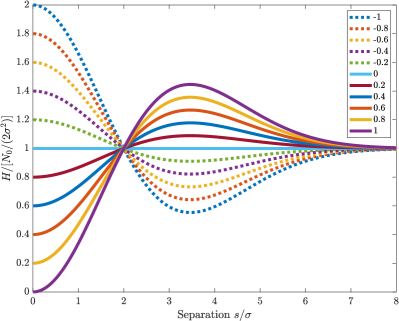
Figure 1: Total Fisher information in Hermite-Gaussian modes up to $q=20$ versus the separation for various values of $\gamma$ (denoted by the legend).

In fact, Fig. 1 even shows an enhancement for sub-Rayleigh anticorrelated sources. This is consistent with the intuitive explanation of how SPADE enhances the Fisher information Tsang et al. (2016a): For $s\ll\sigma$, the $q=1$ mode is the most sensitive to the separation parameter, while the $q=0$ mode, which contributes mostly background noise to direct imaging, is filtered by SPADE. If the sources are close and anticorrelated, the coupling to the $q=1$ mode is enhanced, so the information is also enhanced.

There are at least two problems with Ref. Larson and Saleh (2018) that can explain the disagreement. One is parametrization. Instead of dealing with the degree of coherence $\gamma$ directly, Ref. Larson and Saleh (2018) defines another parameter $p$, which is related to $\gamma$ through Eq. (13) in Ref. Larson and Saleh (2018). Every curve plotted in Ref. Larson and Saleh (2018) assumes a fixed $p$ rather than $\gamma$. The problem is that fixing $p$ leads to an unphysical dependence of $\gamma$ on the separation, as shown in Fig. 2. It is unclear what sources in practice can exhibit such behaviors, which look especially bizarre in the case of $\gamma<0$: the sources acquire significant anticorrelation as they get closer and achieve perfect anticorrelation at $s=0$, even for moderate levels of $p$. Thus any result that assumes a fixed $p$ can be misleading.

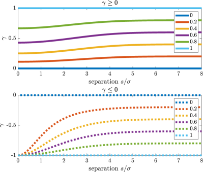
Figure 2: Plots of the degree of coherence $\gamma$ versus separation $s$ for various values of $p$ (denoted by the legends), according to Eq. (13) in Ref. Larson and Saleh (2018). The Gaussian point-spread function is assumed.

The other problem with Ref. Larson and Saleh (2018) is its use of a normalized one-photon density operator in the computation of the quantum Fisher information (QFI). While the use is justified for incoherent sources Tsang et al. (2016a); Ang et al. (2017); *tsang16c; *tsang18, it can lead to incorrect results otherwise. For a weak thermal state with $M$ temporal modes, the density operator for each temporal mode can be approximated as $\rho=(1-\epsilon)\rho_{0}+\epsilon\rho_{1}$, where $\rho_{0}$ is the vacuum state, $\rho_{1}$ is the one-photon state, and $\epsilon\ll 1$ is the expected photon number per temporal mode, given by $\epsilon=\int_{-\infty}^{\infty}dx\Gamma(x,x)/M$ Tsang et al. (2016a). For the incoherent sources assumed in Refs. Tsang et al. (2016a); Ang et al. (2017); *tsang16c; *tsang18, $\epsilon$ does not depend on the parameters of interest $\theta$, so the QFI in $\rho$, defined as $Q(\rho)$, is simply $\epsilon Q(\rho_{1})$. For partially coherent sources, however, $\epsilon$ can depend on the parameters because of interference. With $\rho_{0}$ being independent of any parameter and $\rho_{0}$ and $\rho_{1}$ living in orthogonal subspaces, it is not difficult to show that

$$Q(\rho) =\epsilon Q(\rho_{1})+J(\epsilon),$$ (7)

where $J$ is the classical information for the distribution $\{1-\epsilon,\epsilon\}$ given by

$$J_{\mu\nu}(\epsilon) =\frac{1}{\epsilon(1-\epsilon)}\frac{\partial\epsilon}{\partial\theta_{\mu}}\frac{\partial\epsilon}{\partial\theta_{\nu}}\approx\frac{1}{\epsilon}\frac{\partial\epsilon}{\partial\theta_{\mu}}\frac{\partial\epsilon}{\partial\theta_{\nu}}.$$ (8)

Even if the QFI is evaluated on a per-photon basis as $Q(\rho)/\epsilon=Q(\rho_{1})+J(\epsilon)/\epsilon$, $J(\epsilon)/\epsilon$ may not be negligible. By ignoring $J(\epsilon)/\epsilon$ and considering only $Q(\rho_{1})$, Ref. Larson and Saleh (2018) must have underestimated the total information for partially coherent sources.

Our final issue with Ref. Larson and Saleh (2018) is its claim that the wavelength-scale coherence length of Lambertian sources Mandel and Wolf (1995) can be important, when the opposite is much more likely for fluorescence microscopy and observational astronomy—two of the biggest applications of incoherent imaging. First of all, the Lambertian model is well known to be heuristic and does not take into account the detailed physics of the emitters. It would be a major surprise if the fluorescent emissions of different particles in common microscopy could exhibit any cooperative effect and acquire coherence at the object plane, contrary to the incoherence assumption widely adopted in fluorescence microscopy Pawley (2006). Second, a wavelength-scale coherence length can hardly be relevant to observational astronomy, as the numerical aperture (NA) is extremely low and the wavelength $\lambda$ is smaller than the characteristic length scale $\sigma\sim\lambda/\textrm{NA}$ by many orders of magnitude. Third, while it is true that spatial coherence develops in the field during diffraction even for spatially incoherent sources by virtue of the Van Cittert-Zernike theorem Mandel and Wolf (1995), the effect has already been properly incorporated in the model used in Refs. Tsang et al. (2016a, b); Tsang (2018a); Ang et al. (2017); *tsang16c; *tsang18, and one should not confuse this effect with partial coherence at the sources.

In conclusion, spatial coherence of the sources is unlikely to be significant in key applications of incoherent imaging, and even if it is, Ref. Larson and Saleh (2018) has overblown its detrimental effect.

This work is supported by the Singapore Ministry of Education Academic Research Fund Tier 1 Project R-263-000-C06-112.

References

- Larson and Saleh (2018) W. Larson and B. E. A. Saleh, Optica 5, 1382 (2018).
- Tsang et al. (2016a) M. Tsang, R. Nair, and X.-M. Lu, Physical Review X 6, 031033 (2016a).
- Tsang et al. (2016b) M. Tsang, R. Nair, and X.-M. Lu, in Proc. SPIE, Quantum and Nonlinear Optics IV, Vol. 10029 (SPIE, Bellingham, WA, 2016) p. 1002903.
- Tsang (2018a) M. Tsang, Physical Review A 97, 023830 (2018a).
- Mandel and Wolf (1995) L. Mandel and E. Wolf, Optical Coherence and Quantum Optics (Cambridge University Press, Cambridge, 1995).
- Goodman (1985) J. W. Goodman, Statistical Optics (Wiley, New York, 1985).
- Pawley (2006) J. B. Pawley, ed., Handbook of Biological Confocal Microscopy (Springer, New York, 2006).
- Tsang (2015) M. Tsang, Optica 2, 646 (2015).
- Ang et al. (2017) S. Z. Ang, R. Nair, and M. Tsang, Physical Review A 95, 063847 (2017).
- Tsang (2017) M. Tsang, New Journal of Physics 19, 023054 (2017).
- Tsang (2018b) M. Tsang, arXiv:1806.02781 [physics, physics:quant-ph] (2018b).