Spectropolarimetry of Seyfert 1 galaxies with equatorial scattering: Black hole masses and Broad Line Region characteristics

Abstract

Here we present the spectropolarimetric observations of a sample of 30 Type 1 AGNs and an analysis of the observed polarization in these AGNs. The observations have been performed with the 6-meter telescope of SAO RAS using the modified SCORPIO-2 spectropolarimeter. We measured the Stokes parameters for the continuum and the broad H$\alpha$ line and obtained the values of polarization degree and the angle of polarization. We found that equatorial scattering is dominant polarization mechanism in the sample, that allows us to use the observed polarization in the broad lines for determination of the central black hole (BH) masses and characteristics (the inclination and emissivity) of the Broad Line Region (BLR). We demonstrated that the recently proposed method of Afanasiev & Popović (2015) for BH mass measurement gives accurate BH masses which are in a good correlation with the stellar velocity dispersion, and consequently the masses determined by the polarization method can be used with calibration purposes. Additionally we found that the BLR in the sample of 30 AGN has an averaged inclination of $35^{\circ}\pm 9^{\circ}$ (mostly between 20 and 40 degrees) and emissivity $\alpha\sim-0.57$ that is more flat than one expected for the classical accretion disc $\alpha\sim-0.75$.

1 Introduction

The unified model of active galactic nuclei (AGN) established after detection of a polarized broad H$\alpha$ line component in the spectrum of the Seyfert 2 (Sy2) galaxy NGC 1068 (Antonucci & Miller, 1985). This indicates that the nature of Seyfert 1 (Sy 1) and Seyfert 2 galaxies is probably the same, but the emission from Sy 2 galaxies is blocked by the torus (Antonucci, 1993). The polarization in the continuum of Sy 2 is due to polar scattering, but the broad emission component observed in some Sy 2 galaxies is coming from the equatorial scattering, where emitted light from the Broad Line Region (BLR) is scattered on the inner part of the torus. Moreover, many of Sy 2 galaxies show the polarized broad lines in their spectra (see e.g. Miller & Goodrich, 1990; Tran et al., 1992; Young et al., 1996; Heisler et al., 1997; Moran et al., 2000; Tran, 2001; Kishimoto et al., 2002a, b; Tran, 2003; Lumsden et al., 2004; Ramos Almeida et al., 2016, etc.).

This discovery establishes the spectropolarimetry as a powerful tool for investigations of the AGN nature, especially in the case of the Type 1 AGNs with prominent broad emission lines (BELs) emitted by a BLR that is supposed to be very close to the central black hole (BH). The BLR has a geometry which is probably driven by the central BH, and this reflects the broad line shapes and parameters that can be used for estimation of the central BH mass (see e.g. Peterson, 2014, for a review). However, there are several problems in using the broad spectral lines for BH mass determination, one of them is that the BLR is very small in size (from several 10s to several 100s light days), with an angular dimension $<10^{-5}$ arcsec for nearest AGNs (Bentz & Katz, 2015) that cannot be resolved with the most powerful telescopes. Consequently, the BLR properties are far from being well characterized, and some of these properties have a strong impact on black hole mass determination. For example, the BLR inclination and geometry (see Collin et al., 2006) may strongly affect the broad-line profiles, especially Full Width at Half Maximum (FWHM) used in the reverberation method. The reverberation method depends on the FWHM, and virial factor $f$ - that strongly depends on the BLR inclination (see Peterson, 2014). The uncertainties of the $f$ and FWHM values can cause large uncertainties in mass determination by the reverberation method. Therefore, it is very important to investigate the BLR nature, and spectroscopy in combination with the measured polarization the BELs that can give us some additional information about it (Gaskell & Goosmann, 2013).

The BLR is supposed to have flattened shape, and the BLR emitting gas is probably following a Keplerian-like motion. It is assumed that the BLR has a clumpy structure, i.e. that it is composed from a number of clouds which radiate isotropically, consequently one cannot expect polarization due to the radiative transfer in the BLR. However, the polarization in the BELs can be due to the scattering of BEL light in the inner part of the torus, i.e. the so-called equatorial scattering (Smith et al., 2004, 2005; Afanasiev et al., 2014a, 2015).

This mechanism of polarization can provide more information about the BLR geometry, and, as it has been shown recently by Afanasiev & Popović (2015) the polarization in BELs can be used for the mass measurement of the central BH in AGNs. The mass determination by polarization method does not depend on the BLR inclination (see Afanasiev & Popović, 2015), and small velocity outflows/inflows do not affect significantly the estimated BH masses (see Savić et al., 2018, for more detailed discussion). Moreover, opposite to with the reverberation method, where the BLR virialization is assumed a priori, in the spectropolarimetric method the Keplerian motion can be checked by using the relationship between the polarization angle and velocities across the broad line profile (Afanasiev & Popović, 2015). All these stated above is in a favor for using spectropolarimetric method to measure BH masses in the Type 1 AGNs.

Moreover, as we will demonstrate in the paper later, the polarization in the broad emission lines can be used for the BLR inclination estimates.

The line profile reflects the characteristics of the velocity field in BLR, and consequently polarization across the broad line profiles can be used for investigation of the BLR structure (Martel, 1998; Smith et al., 2002, 2004, 2005; Goosmann & Gaskell, 2007; Afanasiev et al., 2014a, 2015). We observe a sample of Type 1 AGNs in order to investigate the BLR nature (inclination and emissivity) and measure the BH masses.

In this paper we present new observations of a sample of 30 Type 1 AGNs with 6-m BTA telescope, which some of them have been observed in Spectropolarimetric monitoring campaign of AGN (Afanasiev et al., 2011, 2014a, 2015). The aim of this paper is to discuss the spectropolarimetric characteristics of Type 1 AGNs in the continuum and BELs. Special attention is paid to the new way of usingpolarization in the broad lines to find some characteristics of BLRs, as e.g. inclination and emissivity. The paper is organized as following: in §2 we describe observations and data reduction, in §3 the results are given and analyzed in §4. Finally, in §5 we present a short discussion and outline our conclusions.

2 Observations and data reduction

The observations have been performed with 6-m telescope of SAO RAS. We used the modified SCORPIO-2 spectrograph (Afanasiev & Moiseev, 2011; Afanasiev et al., 2014b) in the spectropolarimetry mode . The log of observations is presented in Table 1, where the name of objects, the redshift, the date of observations, the exposure and the seeing are give. A double Wollaston prism - WOLL2 (Oliva, 1997) is used as a polarization analyzer. In this analyzer the rays that enter into two Wollastons which have crystal axis at $45^{\circ}$, and emerge at 4 different angles with relative intensities depending on the polarization angle and degree of the input light. The four images correspond therefore to measurements performed with polarizers at 0, 90, 45 and 135 degrees. The obtained couple images of an object are distributed along the slit using achromatic wedges. In each exposition the four spectra have been recorded simultaneously in different polarization planes. Thus, we can measure three Stokes parameters I, Q and U, from only one observation, unlike a single Wollaston analyzer usage, demanding to obtain four exposures in different angles of polarization plane.

Table 1: Summary log of observations. From the left to the right are given: name of object, redshift, date of observations, exposure in sec and seeing in arcsec.

Object	z	Date	Exposure	Seeing
		dd/mm/yy	(sec)	(arcsec)
Mkn335	0.026	09/11/13	2400	1.1
Mkn1501	0.098	20/11/14	3600	1.2
Mkn1148	0.064	20/11/14	2880	1.2
1Zw1	0.059	22/11/14	2400	2.5
IRAS03450+0055	0.031	20/10/14	3600	2.0
3C120	0.033	06/11/13	3600	2.9
Akn120	0.032	24/03/14	3600	1.5
MCG+08-11-011	0.020	06/11/15	3600	1.0
Mkn6	0.019	25/02/13	5400	2.5
Mkn79	0.022	07/12/15	3600	1.1
PG0844+349	0.064	07/04/16	3600	1.3
Mkn704	0.029	23/11/14	3420	2.5
Mkn110	0.035	12/11/14	2400	1.1
NGC3227	0.004	10/12/15	1800	1.0
NGC4051	0.002	24/03/14	1800	1.5
NGC4151	0.003	23/05/14	1200	1.5
3C273	0.158	25/03/14	1440	1.5
NGC4593	0.009	18/03/15	1800	2.0
Mkn231	0.042	18/03/15	1800	1.8
IRAS13349+2438	0.108	23/05/14	2400	1.3
Mkn668	0.077	24/03/15	5400	2.5
NGC5548	0.017	25/03/14	2400	1.5
Mkn817	0.031	29/05/14	3600	1.2
Mkn841	0.036	29/05/14	4200	1.1
Mkn876	0.129	26/03/15	3900	2.0
PG1700+518	0.292	05/04/16	3600	1.7
3C390.3	0.056	09/05/14	3600	1.0
Mkn509	0.034	21/10/14	3360	1.9
Mkn304	0.066	09/11/13	3600	1.1
3C445	0.056	05/11/13	3600	1.5

Figure 1: Comparison of observed values in V(5500Å) waveband and ones given in literature of the polarization degree (left) and polarization angle (right) for polarization standard stars.

In this mode, the slit length is 1 arcmin. The width of the slit, depending the seeing, was between 1.5 and 2 arcsec. The spectral resolution is caused by the width of the slit and used spectral grating. Typical spectral resolution was 8-11 Å. We used two gratings - VPHG940 (spectral coverage 4000-7500 ÅÅ) and VPHG1026 (spectral coverage 5800-9500 ÅÅ). Unlike conventional diffraction gratings in the case of VPHG, the difference between polarization in directions parallel and perpendicular to the direction of dispersion is small (about 5%). This makes VPHG very suitable for spectrophotometric observations.

For the WOLL2 analyzer three Stokes parameters have been found using following relations:

$$I(\lambda)=I_{0}(\lambda)+I_{90}(\lambda)K_{Q}(\lambda)+I_{45}(\lambda)+I_{135}(\lambda)K_{U}(\lambda)$$

$$Q(\lambda)={I_{0}(\lambda)-I_{90}(\lambda)K_{Q}(\lambda)\over{I_{0}(\lambda)+I_{90}(\lambda)K_{Q}(\lambda)}},$$

$$U(\lambda)={I_{45}(\lambda)-I_{135}(\lambda)K_{U}(\lambda)\over{I_{45}(\lambda)+I_{135}(\lambda)K_{U}(\lambda)}},$$

where $K_{Q}$ and $K_{U}$ are the instrumental parameters related to the transmission of the polarization channels. Each channel has been corrected for spectral sensitivity of the device, which is determined from observations of the polarization standards. The $I_{0}(\lambda),\ I_{90}(\lambda)),\ I_{45}(\lambda)$ and $I_{135}(\lambda)$ are the intensity in the four polarization angles.

The degree of linear polarization $P(\lambda)$ and polarization angle $\varphi(\lambda)$ have been obtained using following relations:

$$P(\lambda)=\sqrt{Q(\lambda)^{2}+U(\lambda)^{2}},\ \ \ \ \varphi(\lambda)={1\over 2}{\rm arctg}[U(\lambda)/Q(\lambda)]+\varphi_{0},$$

where $\varphi_{0}$ is the zero point of polarization angle, which also has been determined by the observations the polarization standards.

Observations for each object have been performed in a series of exposures (more than 5), with the integration aperture of 2$\times$10 arcsec. Before or after the object exposure, polarization standards and zero-polarization stars have been observed (the standards are taken from Turnshek et al., 1990; Hsu & Breger, 1982). The typical object exposures are 180-240 seconds that depends on the object brightness. This type of observations allowed us to have a robust statistical estimation of the observed values (see Afanasieva, 2016, for a detailed discussion). The method of observations and data reduction was described in more details by Afanasiev & Amirkhanyan (2012). In the case when the galactic latitude was smaller than 25 degrees, we took into account the interstellar polarization as an average polarization of several stars around the observed object, as it was described by Afanasiev et al. (2014a). The accuracy of our observation is limited by the variation of the depolarization in the Earth atmosphere.

In Fig. 1 we give our measurements of the polarization degree and polarization angle ($P_{obs}$ and $PA_{obs}$) for the standard polarization of stars, and compare our measurements with those given in the literature ($P_{tab}$ and $PA_{tab}$ taken from Schmidt et al., 1992). The error of the measurements of polarization is ($P_{tab}-P_{obs}$) $\sim$ 0.2%, and the polarization angle around ($PA_{tab}-PA_{obs}$) $\sim$ 3 degrees.

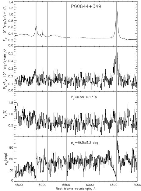
Figure 2: Spectropolarimetric observations of quasar PG0844+349, from the top to the bottom: integral spectrum, polarized spectrum, degree of polarization and polarization angle. The vertical lines denote the position (from left to the right) of H$\beta$, continuum at $\lambda$5100 Å  continuum at $\lambda$5500 Å  and H$\alpha$ line

.

Table 2: The data for the continuum polarization. From the left to the right are given: object name, flux at 5100 Å  measured from our observations, unbiased degree of polarization in two wavebands $V(5500\AA)$ and $R(6500\AA)$, index $n$ of the wavelength dependent slope, polarization angles for $V(5500\AA)$ and $R(6500\AA)$ wavebands, $P(ref)$ and $PA(ref)$ are the polaization degree and angle taken from reference given in column ’Ref’ in the V-band.

Object	Flux(5100)	$P(V)$	$P(R)$	$n$	$\varphi(V)$	$\varphi(R)$	$P(ref)$	$PA(ref)$	Ref
Mkn335	7.53$\pm$0.54	0.41$\pm$0.14	0.36$\pm$0.06	-0.78$\pm$0.49	110.9$\pm$14.9	98.9$\pm$5.9	0.48$\pm$0.11	107.6$\pm$6.9	1
Mkn1501	1.59$\pm$0.46	0.94$\pm$0.34	1.25$\pm$0.60	1.71$\pm$0.90	140.9$\pm$16.2	153.4$\pm$12.6
Mkn1148	1.38$\pm$0.15	0.67$\pm$0.22	0.98$\pm$0.45	2.28$\pm$0.85	67.1$\pm$11.1	81.0$\pm$16.2	0.81$\pm$0.28	77$\pm$10	2
1Zw1	8.21$\pm$1.02	0.91$\pm$0.21	0.77$\pm$0.16	-1.00$\pm$0.44	146.7$\pm$ 8.4	149.6$\pm$ 6.5	0.70$\pm$0.05	148$\pm$2	1
IRAS03450+0055	3.15$\pm$0.26	0.93$\pm$0.24	0.86$\pm$0.34	-0.47$\pm$0.72	115.9$\pm$ 7.8	119.5$\pm$11.0
3C120	6.38$\pm$0.38	1.17$\pm$0.25	1.10$\pm$0.24	-0.37$\pm$0.44	111.4$\pm$ 6.6	103.5$\pm$7.9	0.92$\pm$0.25	103.5$\pm$7.9	4
Akn120	7.91$\pm$0.44	0.59$\pm$0.17	0.70$\pm$0.29	1.02$\pm$0.76	78.7$\pm$ 6.9	70.9$\pm$ 8.9	0.65$\pm$0.13	78.6$\pm$5.7	4
MCG+08-11+011	5.73$\pm$0.36	1.38$\pm$0.15	1.36$\pm$0.25	-0.09$\pm$0.33	71.9$\pm$ 3.6	76.6$\pm$ 5.9	1.69$\pm$0.46	76.4$\pm$19	4
Mkn6	8.96$\pm$0.63	0.71$\pm$0.20	0.78$\pm$0.16	0.56$\pm$0.47	155.2$\pm$ 9.3	148.2$\pm$ 8.0	0.90$\pm$0.02	156.5$\pm$0.8	1
Mkn79	3.64$\pm$0.22	1.43$\pm$0.24	1.20$\pm$0.22	-1.05$\pm$0.36	4.2$\pm$ 4.6	-0.2$\pm$11.5	1.34$\pm$0.19	0.4$\pm$16.2	4
PG0844+349	2.97$\pm$0.15	0.58$\pm$0.17	0.58$\pm$0.20	0.00$\pm$0.66	49.5$\pm$ 5.2	49.1$\pm$ 9.8
Mkn704	3.89$\pm$0.24	2.32$\pm$0.36	2.21$\pm$0.41	-0.29$\pm$0.36	58.3$\pm$ 2.6	56.8$\pm$ 5.3	2.01$\pm$0.21	68.1$\pm$5.1	3
Mkn110	3.69$\pm$0.28	0.55$\pm$0.16	0.38$\pm$0.23	-2.21$\pm$1.05	19.2$\pm$ 0.5	21.8$\pm$ 7.3	0.21$\pm$0.13	18.$\pm$15.	2
NGC3227	10.32$\pm$1.97	1.25$\pm$0.42	0.96$\pm$0.29	-1.58$\pm$0.64	137.8$\pm$11.2	142.2$\pm$13.2	1.3$\pm$0.1	133$\pm$3.	5
NGC4151	40.52$\pm$7.97	0.32$\pm$0.30	0.20$\pm$0.11	-2.81$\pm$2.78	69.7$\pm$ 6.2	68.2$\pm$ 6.3	0.26$\pm$0.08	62.8$\pm$8.4	4
NGC4051	17.78$\pm$1.24	0.39$\pm$0.19	0.22$\pm$0.21	-3.43$\pm$1.67	92.6$\pm$10.2	98.2$\pm$ 3.4	0.87$\pm$0.04	78.0$\pm$0.8	4
3C273	26.61$\pm$1.61	1.11$\pm$0.17	1.34$\pm$0.34	1.13$\pm$0.45	57.8$\pm$ 4.2	61.3$\pm$ 3.9	0.87$\pm$0.11	65$\pm$3	8
NGC4593	10.87$\pm$0.56	0.77$\pm$0.20	0.62$\pm$0.08	-1.30$\pm$0.37	106.9$\pm$ 9.6	101.6$\pm$10.8	0.57$\pm$0.16	109.5$\pm$11.	2
Mkn231	8.88$\pm$0.40	3.29$\pm$0.29	2.98$\pm$0.63	-0.59$\pm$0.36	118.4$\pm$ 3.3	118.8$\pm$ 6.8	2.87$\pm$0.08	95.1$\pm$1.	4
IRAS13349+2438	5.23$\pm$0.20	5.59$\pm$0.27	5.42$\pm$0.39	-0.18$\pm$0.13	125.5$\pm$ 0.9	126.2$\pm$ 3.7	5.70$\pm$0.12	124.4$\pm$0.7	9
Mkn668	1.87$\pm$0.18	1.06$\pm$0.22	0.91$\pm$0.32	-0.91$\pm$0.63	127.7$\pm$ 5.6	136.6$\pm$13.2	0.91$\pm$0.55	145$\pm$3	7
NGC5548	9.49$\pm$0.39	0.50$\pm$0.12	0.40$\pm$0.15	-1.34$\pm$0.68	34.2$\pm$ 5.1	34.7$\pm$ 5.7	0.72$\pm$0.10	33.5$\pm$3.9	2
Mkn817	3.86$\pm$0.15	0.71$\pm$0.15	0.57$\pm$0.21	-1.31$\pm$0.65	76.4$\pm$ 7.7	77.9$\pm$18.0
Mkn841	5.30$\pm$0.08	0.78$\pm$0.33	1.13$\pm$0.38	2.22$\pm$0.75	100.7$\pm$14.8	102.3$\pm$12.8	1.00$\pm$0.03	92.9$\pm$4.3	4
Mkn876	3.37$\pm$0.07	0.94$\pm$0.23	0.78$\pm$0.19	-1.12$\pm$0.49	113.8$\pm$ 9.4	111.5$\pm$13.6	0.81$\pm$0.04	110.5$\pm$3.7	1
PG1700+518	3.10$\pm$0.10	0.77$\pm$0.22	0.89$\pm$0.35	0.87$\pm$0.73	71.7$\pm$12.7	53.0$\pm$15.5	0.54$\pm$0.10	56$\pm$5	10
3C390.3	1.69$\pm$0.08	0.77$\pm$0.08	0.91$\pm$0.37	1.00$\pm$0.68	139.5$\pm$ 0.8	141.6$\pm$ 7.7	0.74$\pm$0.3	146$\pm$5	6
Mkn509	7.15$\pm$0.28	0.68$\pm$0.15	0.52$\pm$0.34	-1.61$\pm$1.10	149.1$\pm$ 7.2	150.7$\pm$ 7.5	1.09$\pm$0.15	146.5$\pm$4.0	4
Mkn304	3.62$\pm$0.57	0.58$\pm$0.20	0.61$\pm$0.11	0.30$\pm$0.50	131.1$\pm$11.3	130.2$\pm$ 6.0	0.98$\pm$0.14	136.6$\pm$4.2	4
3C445	1.18$\pm$0.06	2.86$\pm$0.55	1.98$\pm$0.58	-2.20$\pm$0.53	152.2$\pm$ 4.2	147.4$\pm$10.5	3.01$\pm$0.30	150$\pm$5	6

UNITS: Flux(5100) is given in $10^{-15}\rm erg\ cm^{-2}s^{-1}\AA^{-1}$, $P(V)$ and $P(R)$ in percents, $\varphi(V)$ and $\varphi(R)$ in degrees

References : 1 - Smith et al. (2002), 2 - Berriman et al. (1990), 3 - Goodrich and Miller (1994), 4 - Martin et al. (1983), 5 - Schmidt and Miller (1985), 6 - Kay et al. (1999), 7 - Corbett et al. (1998) , 8 - Wills at al. (1992a), 9 - Wills at al. (1992b)

The observed spectra have been corrected to the system sensitivity function and extinction. The flux calibration (given in erg s^-1cm^-2A^-1) is performed by using the spectrophotometic standards (in this case we used the spectra of G191b2b, BD+28d4655 and BD+33d2642 stars). The continuum at 5100 Å and measurements of the polarization parameters from our spectra are given in Table 2.

The typical spectra are shown in Fig. 2, where we present (from top to bottom) the unpolarized and polarized spectra, the degree of polarization and the polarization angle for quasar PG0844+349. The wavelengths are rescaled to the rest-frame. The vertical lines denote the position of the H$\beta$ and H$\alpha$ lines and the spectral region of the unpolarized continuum measurement at 5100 Å and polarized one at 5500 Å.

3 Results

We analyzed our observations in order to give the polarization parameters in the continuum and broad lines. As it can be seen in Fig. 2 we can detect the H$\beta$ and H$\alpha$ broad lines in polarized light, however H$\beta$ is generally weaker and S/N ratio in the polarized light is smaller than in H$\alpha$. Therefore, we will use the polarized H$\alpha$ line to measure parameters in broad lines. Our measurements are given in Tables 2 and 3 and Figs. 4 – 9. We separately discuss the obtained polarization parameters in the continuum and lines.

3.1 Polarization in the continuum

The estimation of the polarization in the continuum is presented in Table 2, where we give the object name (1st column), the observed fluxes at 5100Å in the aperture 2$\times$10 arcsec in units of $10^{-15}\rm erg\ cm^{-2}s^{-1}\AA^{-1}$ (2nd column). The spectra of nucleus were obtained by subtracting the host galaxy spectrum from the observed one using the technique described by Afanasiev et al. (2014b). Properties of the continuum polarization for each object were defined as follows. Assuming that $V(5500\AA)$ waveband covers the wavelength interval of $\lambda\lambda=5300-5700\AA$, and $R(6500\AA)$ interval $\lambda\lambda=6300-6700\AA$ (in the rest frame). In Table 2 we offer the averaged values of polarization degree (column 3rd and 4 th) in these intervals (P(V) and P(R)) in percents. In cases where the measured polarization degree was on the level of its error, the P(V) and P(R) values are biased. In Table 2 we give unbiased values of the degree of polarization, which were calculated as (see Simmons and Stewart, 1985):

$$P_{unbiased}=\sqrt{P^{2}-1.41\sigma_{P}^{2}},$$

where $P$ is the measured polarization and $\sigma_{P}$ is the corresponding error. We also find the index $n$ (that has been defined by Afanasiev et al., 2011) which indicates the dependence of polarization as $P\sim\lambda^{n}$. Index $n$, which represents the inclination of polarized continuum, was calculated using the measured polarization in $V(5500\AA)$ and $R(6500\AA)$ wavebands as:

$$n={{\log P(V)-\log P(R)}\over\log(5500/6500)}.$$

The index $n$ in the first approximation describes the depolarization of the radiation as a function of wavelengths and can be used for the exploring of the polarization mechanisms. For example, if the observed polarization is caused by Thompson scattering due to radiation transfer then it does not depend from wavelength,while if there is a wavelength dependence of polarization in the continuum, one has to suppose other mechanisms to explain it. The index $n$ and polarization angles for V- and R-bands are given in Table 2 – columns 5th, 6th and 7th respectively. Several of AGNs from our sample, polarization degrees and angles have been observed earlier in the optical V-band. We show these data in Table 2 (columns 8th and 9th, for polarization degree and angle, respectively) and in the 10th column we quote the corresponding reference. In Fig. 3 we compare our measurements and those given in literature. As one can see in Fig. 3, there are no systematic differences between our and data  taken from literature. The scatter between our data and data from literature is probably due to measurement errors and possible variability of objects.

Figure 3: Comparison of our measurements in V(5500Å) waveband with ones given in literature: the degree of polarization (left) the angle (right)

3.2 Polarization in the broad lines

As we mentioned above, we expect that a dominant polarization mechanism in the BLR light is the equatorial scattering (see Smith et al., 2005; Afanasiev & Popović, 2015). In the case of the equatorial scattering, and Keplerian-like motion of broad line emitting gas, the polarization angle has specific shape (see Afanasiev et al., 2014a; Afanasiev & Popović, 2015). The horizontal S-like shape of polarization angle in H$\beta$ and H$\alpha$ can be detected in all observed objects. The spectral and polarization parameters around H$\alpha$ for each object were measured (see Figs. 4-9).

In Figs.4-9 we show the top to bottom: the H$\alpha$ line profile, the parameters $Q$ and $U$ across the line profile, the degree of polarization ($P$) and polarization angle ($\Delta\varphi$) across the line profile

The averaged parameters of $<Q>$, $<U>$, $<P>$ and $<\varphi>$ measured in the continuum around the H$\alpha$ line (R-band) are given on the corresponding plot.

3.2.1 Estimates of BH masses

It was shown in Afanasiev et al. (2014a) and Afanasiev & Popović (2015) that in the case of the Keplerian-like motion (and equatorial scattering of the BLR light) the velocities across the broad line and $\tan\varphi$ are connected as (see Fig. 10):

$$\log({V_{i}\over c})=a-b\cdot\log(\tan(\Delta\varphi_{i})),$$

where $c$ is the speed of light, and constant $a$ depends on the BH mass ($M_{BH}$) as

$$a=0.5\log\bigl{(}{{GM_{BH}\cos^{2}(\theta)}\over{c^{2}R_{sc}}}\bigr{)}.$$

where $G$ is the gravitational constant, $R_{sc}$ is the distance of the scattering region from the central black hole and $\theta$ is the angle between the BLR disk and the scattering region. In the case of equatorial scattering, we can assume the $\theta\sim 0$ (i.e. $\cos^{2}\theta\sim 1$, see Afanasiev & Popović, 2015; Savić et al., 2018) and therefore, the BH mass is independent from the inclination. $b$ is 0.5 for the case of the Keplerian motion.

The equations above are obtained using the approach of a simple geometric model (see Afanasiev & Popović, 2015), but it is shown in Savić et al. (2018) that this approximation gives good results. In the paper Savić et al. (2018) validity of the method was explored using numerical simulations by applying the modified STOKES code (Marin et al., 2012) showing that the observed rotation of the polarization plane depending on the velocity in the broad emission lines for the Keplerian motion in the BLR. The motion is well described by Eq. (5) and obtained masses are weakly dependent on the geometry of the torus and the inclination of the BLR.

For each AGN from the sample in the corresponding bottom panel in Figs. 4-9 we give a trend between $V/c$ and $\Delta\varphi$ (in the logarithmic scale) which indicates that in all AGNs from a sample the equatorial scattering occurs and that Keplerian-like emission gas can be observed. The arrow on this panels indicate the maximum angle of the polarization plane rotation across the H$\alpha$ line profile. The estimated masses are given in the bottom panel and also in Table 3.

As it can be seen in bottom panels Figs. 4-9, relative change the polarization angle $\Delta\varphi$, mostly follow expected shape in the case of Keplerian motion in the BLR. However, in some of the AGNs from the sample $\Delta\varphi$ as a function of velocity has no clear S-shape (see e.g. of NGC4593, Mrk 231, Mrk 509. etc.), then we estimate the shape, as it is shown in Fig. 10, reproducing the shape assuming the Keplerian motion (assuming $b=0.5$ in Eq. (5), see Afanasiev & Popović, 2015). Fig. 10 demonstrates an example of the analysis of the observed change in the polarization plane angle in the broad H$\alpha$ line for PG0844+349. The observed deviations from the expected dependence $\log(v/c)$vs $\log(\tan\varphi)$ are probably related to the presence of a non-circular motion in the BLR disc, as it was found in the galaxy Mkn6 (Afanasiev et al., 2014a).

Additionally, we carefully consider some objects where the changes across the H$\alpha$ broad line are not prominent due to other influences, e.g. in the case of 3C390.3 where a strong depolarization was found (see Afanasiev et al., 2015, compare Fig. 1 from the paper with panel in Fig. 9).

In bottom panels of Figs. 4-9 the plots of Eq. (5) with coefficient $a$ and $\log(M/M_{\odot})$ (written on the plots) are given. The full circles are taken from the red and open ones from the blue broad H$\alpha$ side.

3.2.2 The inner scattering radius

The inner dusty torus radius ($R_{sc}$) can be estimated by the reverberation, i.e. by finding the time lag between optical and infrared emission of an AGN (see e.g. Koshida at al., 2014). Comparing the measurements with the luminosity, it was found that $R_{sc}\propto L^{-0.5}$ and that the $R_{sc}$ seems to be about twice as large as the corresponding BLR radius (Kishimoto et al., 2011).

The relationship between $R_{sc}$ and luminosity is expected for a case where the dust temperature and the inner radius of the dusty torus are determined by radiation equilibrium and sublimation of dust, respectively. This dependence has been confirmed by a quantitatively estimated inner radius of the dust torus by taking into account the wavelength dependent efficiency of dust grain absorption (Barvainis,, 1987), where luminosity at $\lambda=1216$Å was used.

In Fig. 11 we show this relationship, which has been calculated using the empirical dependence of the inner radius of the torus on UV luminosity. The correlation of the inner radius of the R_sc torus with UV luminosity is physically justified and confirmed by measurements in the near IR emission. However, it should be noted that the dependence of R_sc – UV flux in literature is confirmed by the extrapolation of the Spectral Energy Distribution (SED) at 1216 Å and also indirectly calculated from the V-color fluxes. To find the luminosity-radius relationship, we used homogeneous GALEX data (F_UV fluxes) measured at $\lambda$ 1516Å.

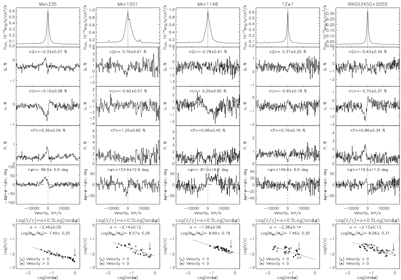
Figure 4: The H$\alpha$ spectral region (1st panel), the shape of Stokes $Q$ and $U$ parameters (2nd and 3rd panels, respectively) across the H$\alpha$ line profile, and corresponding percent of polarization (P%) and polarization angle - $\Delta\varphi$ (4th and 5th panels, respectively). On bottom panels the relationship of $\log(v/c)$ v.s. $\log\tan(\Delta\varphi)$ is shown. From left to the right the (column) panels are for Mkn 335, Mkn 1501, Mkn 1148, 1Zw1 and IRAS03450+0055.

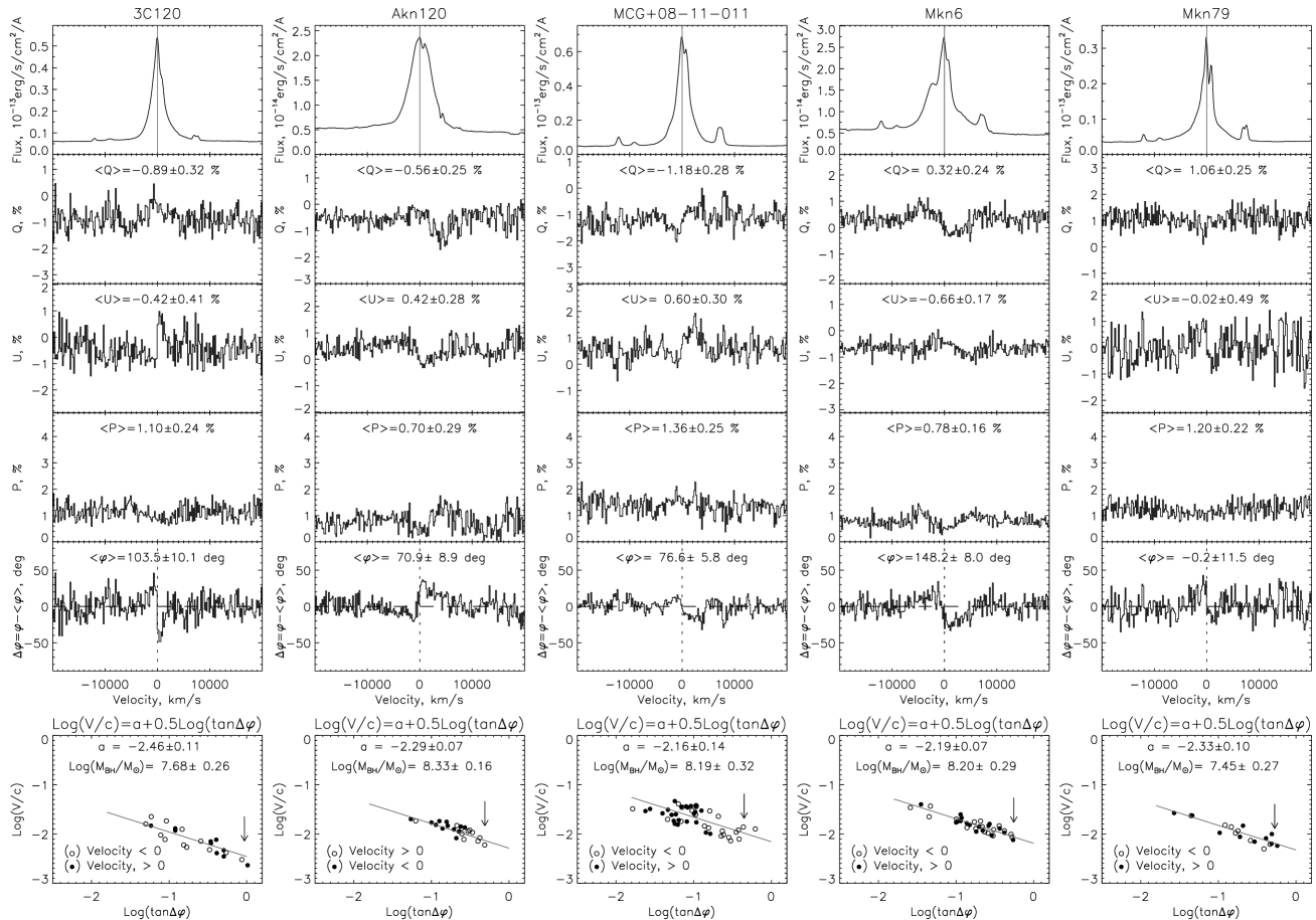
Figure 5: The same as in Fig. 4, but for 3C 120, Akn 120, MCG+08-11-011, Mkn 6 and Mkn 79.

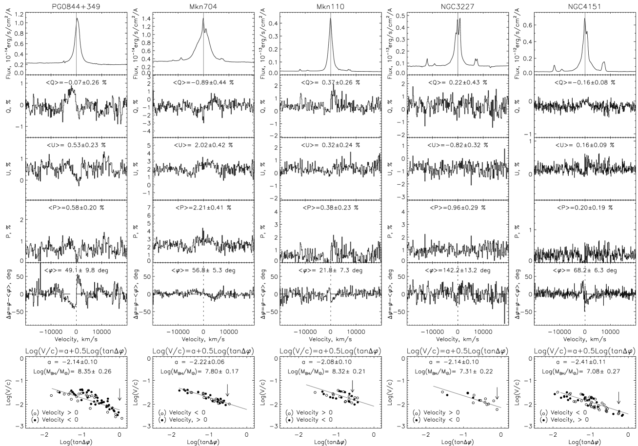
Figure 6: The same as in Fig. 4, but for PG 0844+349, Mkn 704, Mkn 110, NGC 3227 and NGC 4151.

Figure 7: The same as in Fig. 4, but for NGC 4051, 3C 273, NGC 4593, Mkn 231 and IRAS13349+2438.

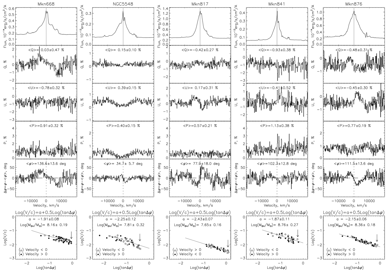
Figure 8: The same as in Fig. 4, but for Mkn 668, NGC 5548, Mkn 817, Mkn 841 and Mkn 876.

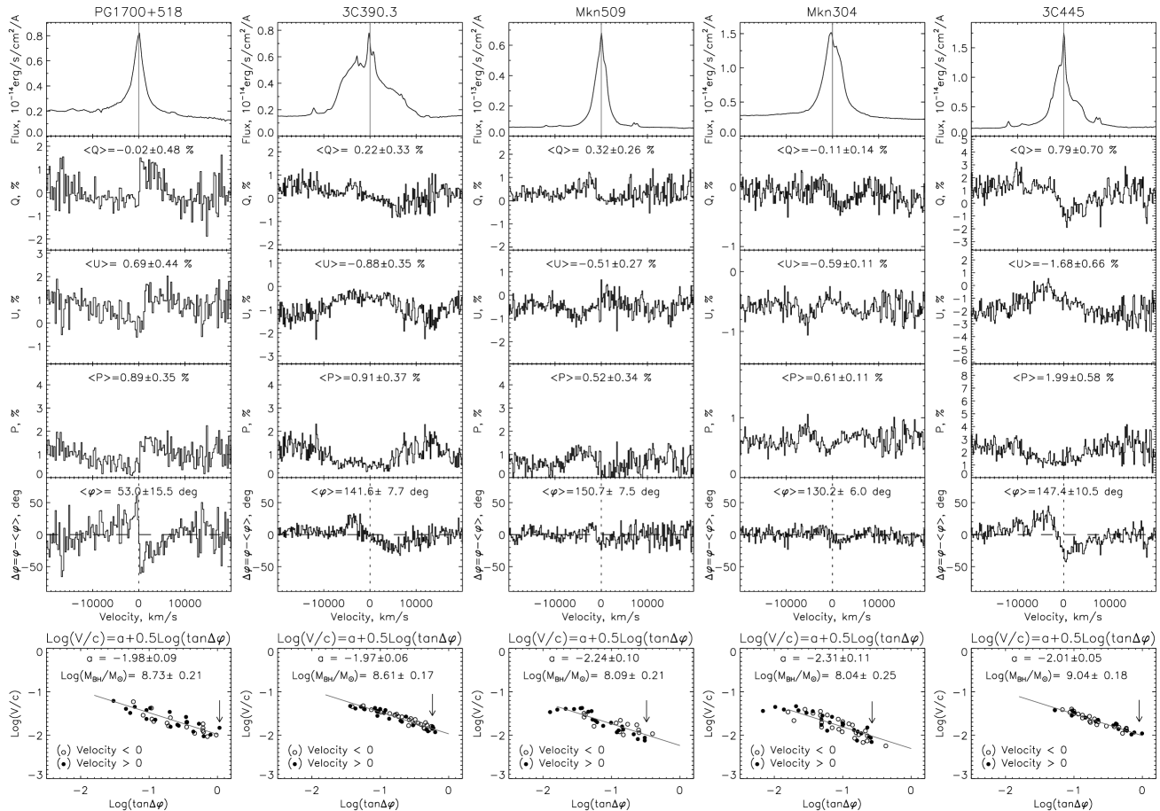
Figure 9: The same as in Fig. 4, but for PG 1700+518, 3C 390.3, Mkn 509, Mkn 304 and 3C 445.

The AB-magnitudes ($m_{AB}$) for AGNs from our sample were taken from NASA/IPAC Extragalactic Database (NED), and then have been converted to the flux using the well-known relationship $\log F_{UV}=-0.4\cdot m_{AB}+7.33$. The absorption is taken into account as $A(F_{UV})=7.9\cdot E(B-V)$ (see Gil de Paz et al., 2007), where $E(B-V)$ is the reddening. For 2/3 of the objects from our sample we could find in literature the UV-fluxes observed with Hubble Space Telescope in $\lambda$1450 Å and $\lambda$1350Å. For a typical energy distribution of Sy1, the systematic difference between the fluxes at $\lambda$1350Å and $\lambda$1516 Å is about 0.06 (in the logarithmic scale). The standard deviation between our data measured at $\lambda$1516Å and taken from the literature at $\lambda$1350 Å  and $\lambda$1450 Å  (Vestergaard, 2002; Kaspi et al., 2005) is in the interval of 0.2-0.25.

As it can be seen in Fig. 11 there is a good correlation between the $R_{sc}$ and luminosity at $\lambda=1516$Å  ($R_{sc}\propto L^{-m}$), where the power index $m$ is 0.421$\pm$0.026. Using this calibration relation, we determined the $R_{sc}$ for those objects for which we could not find the $R_{sc}$ in literature and give these values for all objects in Table 3.

Figure 10: The measured value of polarization across the line profile. An example for PG0844+349, the panel up presents the horizontal S-shaped polarization angle across the H$\alpha$ line profile, the measured (estimated) maximum P.A. is shown on the plot. The panel bottom shows the velocity vs. $\tan(\varphi)$ relation across line (in logarithmic scale).

Figure 11: The empirical dependence of the estimation of the inner radius $R_{sc}$ of the torus on the UV-luminosity $\lambda L(\lambda)$  for $\lambda=1516\AA$ . The gray line shows the power dependence with the power index of 0.421$\pm$0.026.

4 Analysis and discussion of the results

4.1 Polarization in the continuum

Firstly we should note here that there is a wavelength dependent polarization in the continuum. This cannot be due to the Thompson scattering in the disc, since it is not wavelength dependent. The change of the polarization as a function of wavelengths can be caused by three effects: (i) The first mechanism is depolarization by Faraday rotation of the plane of polarization on the length of the electron free path in the magnetic accretion disc (Faraday rotation depolarization, see e.g. Agol & Blaes, 1996; Gnedin & Silant’ev, 1997; Agol et al., 1998). This mechanism gives polarization which depends on wavelengths, the degree of polarization in this case is less than predicted by the radiation transfer mechanism in the accretion disk (Chandrasekhar, 1950); (ii) The second mechanism is the scattering on the torus dust, where, as it is well known, the degree of polarization is maximum at $\lambda_{max}=0.6$ mkm (see Serkowski et al., 1975). For $\lambda<\lambda_{max}$, the polarization is increasing with the wavelength, and for $\lambda>\lambda_{max}$ it is decreasing. The theoretical models show that the continuum polarization due to torus dust scattering is dependent from the wavelengths (Marin et al., 2012), and that for $\lambda<0.8$ mkm it is increasing; (iii) The third effect is described in wo99, where the observed wavelength dependence of the polarization in some AGNs can be explained by dust scattering in the optically thin cone. It is found (from modelling) that the multiple scattering in the cones is important for the optical depth larger than $\sim 0.1$.

It is difficult to separate effects giving the dependence of polarization on the wavelength in continuum, but if we assume that magnetic field in the accretion disc is connected with the mass of central black hole (magnetic coupling model, see e.g. Ma et al., 2007), then we can expect that the index of the continuum slope is a function of the central BH mass, as it has been shown in Afanasiev et al. (2011). We give an empirical relation between the index $n$ and $\log M_{BH}$.

Using the data given in Tables 2 (for measured $n$) and 3 (for measured BH masses) we explored this relation (see Fig. 12). As it can be seen in Fig. 12, only one object (3C445) shows a strong deviation from the expected linear best fit (solid line). The correlation coefficient for all points is 0.79. If we remove the outlier (point representing 3C445) the correlation coefficient increases up to 0.88 for the BH mass range from $10^{7}M\odot$ to $10^{9}M\odot$. The statistical significance of this correlation is $<10^{-3}$. The slope of the obtained dependence is $1.6\pm 0.3$, which is, within the error-bars, in an agreement with the result obtained earlier by Afanasiev et al. (2011). Taking that the Faraday rotation depolarization can give $n\sim\log M_{BH}$ relationship, one can conclude that it has an important role in the continuum depolarization in Type 1 AGNs.

The obtained results show that probably the polarization in the continuum is mainly produced by the accretion disc while the $n$ vs $\log M$ relation points to the magnetic field in accretion disc those dependent on the black hole mass (Agol & Blaes, 1996; Agol et al., 1998), that is expected in the so called magnetic coupling model (Ma et al., 2007). However, one can suppose that a small amount of the polarized light in the continuum is caused by the scattering in the torus or cones, but it is hard to separate these two mechanisms without detail modeling of polarization in the continuum. The polarization of the most of Type 1 AGNs from our sample is between 0.5% – 1% (see Table 2) that is expected for broad line AGNs, however there are four objects showing polarization higher than 2% - IRAS 13349, Mkn 231, 3C 445 and Mkn 704.

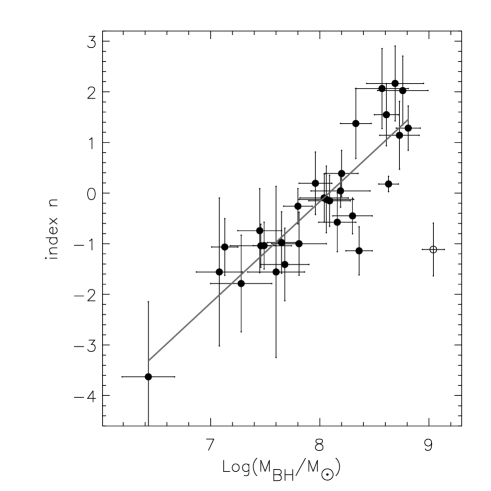
Figure 12: Dependence of index $n$ onthe BH mass.

Table 3: The polarization parameters for H$\alpha$. From left to the right: name of object, logarithm of the UV-luminosity at $\lambda=$1516Å, corresponding reference, $R_{sc}$ - the inner radius of torus, corresponding reference and logarithm of the BH masses (measured by polarization method).

Object	$Log({\lambda}L_{\lambda})$	Ref.	$R_{sc}$	Ref.	$Log\bigl{(}{M_{BH}\over{M_{\odot}}}\bigr{)}$
	$\lambda=1516\AA$		ligth day
Mkn335	43.98$\pm$0.25	4,5	142$\pm$26	2	7.49$\pm$0.25
Mkn1501	44.06$\pm$0.21	4,5	398$\pm$46	1	8.57$\pm$0.26
Mkn1148	44.54$\pm$0.20	4	232$\pm$28	1	8.69$\pm$0.18
1Zw1	44.21$\pm$0.20	4,5	93$\pm$9	2	7.46$\pm$0.30
IRAS03450+0055	44.36$\pm$0.27	4	118$\pm$25	1	8.06$\pm$0.31
3C120	44.57$\pm$0.29	4,5,6	223$\pm$37	1	7.68$\pm$0.26
Akn120	44.77$\pm$0.42	4,5,6	452$\pm$167	3	8.33$\pm$0.16
MCG+08-11+011	44.32$\pm$0.28	4	179$\pm$33	2	8.19$\pm$0.32
Mkn6	44.62$\pm$0.26	4	214$\pm$59	3	8.20$\pm$0.29
Mkn79	42.79$\pm$0.22	4,5,6	71$\pm$14	3	7.45$\pm$0.27
PG0844+349	44.56$\pm$0.25	4,5	236$\pm$25	1	8.35$\pm$0.26
Mkn704	43.62$\pm$0.28	4	98$\pm$13	1	7.80$\pm$0.17
Mkn110	44.31$\pm$0.26	4,5,6	171$\pm$12	3	8.32$\pm$0.21
NGC3227	42.36$\pm$0.30	4,6	22$\pm$2	2	7.31$\pm$0.22
NGC4151	42.92$\pm$0.25	4,5,6	44$\pm$8	3	7.08$\pm$0.27
NGC4051	42.09$\pm$0.28	4,6	25$\pm$4	2	6.43$\pm$0.29
3C273	46.28$\pm$0.31	4,5	963$\pm$291	3	8.81$\pm$0.24
NGC4593	43.24$\pm$0.27	4,6	67$\pm$13	2	7.28$\pm$0.19
Mkn231	44.69$\pm$0.25	4	304$\pm$71	2	8.30$\pm$0.27
IRAS13349+2438	46.04$\pm$0.27	4	1130$\pm$160	3	8.63$\pm$0.15
Mkn668	42.95$\pm$0.23	4	53$\pm$5	1	8.16$\pm$0.19
NGC5548	43.16$\pm$0.25	4,5,6	114$\pm$26	2	7.81$\pm$0.32
Mkn817	44.28$\pm$0.22	4	180$\pm$18	2	7.65$\pm$0.16
Mkn841	44.29$\pm$0.29	4,5	182$\pm$28	1	8.76$\pm$0.27
Mkn876	44.65$\pm$0.27	4,5,6	254$\pm$39	1	8.36$\pm$0.18
PG1700+518	44.73$\pm$0.20	4,6	277$\pm$34	1	8.73$\pm$0.21
3C390.3	44.38$\pm$0.27	4,5,6	200$\pm$29	1	8.61$\pm$0.17
Mkn509	44.55$\pm$0.20	4,5,6	208$\pm$19	3	8.09$\pm$0.21
Mkn304	44.64$\pm$0.24	4	255$\pm$35	1	8.04$\pm$0.25
3C445	45.64$\pm$0.28	4	650$\pm$115	1	9.04$\pm$0.18

References: 1 - this work, 2 - Koshida at al. (2014), 3 - Kishimoto et al. (2011), 4 - GALEX , 5 - Vestergaard (2002), 6 - Kaspi t al. (2005)

4.2 Measurements of BH mass from H$\alpha$ polarization

We used the method given in Afanasiev & Popović (2015) to measure BH masses. The method does not depend of the inclination of the BLR in the case equatorial scattering, and detailed discussion of the method is given in Savić et al. (2018), where the equatorial polarization in the broad lines has been modelled with STOKES code. It seems that the method gives reasonable accurate estimates of BH masses, even if in the BLR some kind of outflows and inflows are present in addition to Keplerian motion, (see in more details in Savić et al., 2018). Also, it was shown in Afanasiev & Popović (2015) that measured BH masses from polarization are in a good agreement with ones obtained by reverberation.

Our measurements of BH masses are presented in Table 3. As it was shown in Tremaine et al (2002) there is a relation between the BH masses and host galaxy bulge stellar velocity dispersion ($\sigma_{*}$) that follows $M_{BH}\sim\sigma_{*}^{4}$. This is caused by well known connection between the brightness of the bulge and stellar velocity dispersion (Faber & Jackson, 1976). We explore this relationship using our BH mass measurements and stellar velocity dispersion given in Onken et al. (2004).

As it can be seen in Fig. 13, the relation between our measurements of BH masses from polarization and stellar velocity dispersions follow expected one. The correlation between BH mass and $\sigma$ is very high (r=0.98).

Our estimates of the BH masses and the relation between $M_{BH}$ and $\sigma$ are in a good agreement with those given by Tremaine et al (2002) and in the future the BH mass measured from polarization in the broad lines can be used for calibration purposes of other methods for BH mass estimation.

Figure 13: Our measurements of BH masses as a function of host galaxy bulge stellar velocity dispersion $\sigma_{*}$ (taken from Onken et al., 2004). The dashed line shows the dependence of $M_{BH}\sim\sigma_{*}^{4}$ taken from Tremaine et al (2002).

We compared the measurements of BH mass given in Table 3 with our previous results by Afanasiev & Popović (2015). It turned out that the latest data have smaller errors than the previous ones, due to our new of the method of simultaneous measurement of Stokes parameters.

4.3 The BLR inclinations

In the case of the reverberation BH mass measurements (also using the relations for single-epoch mass measurements) it is very important to have information about the disc inclination (see Collin et al., 2006). In the polarization method, the BH mass estimates do not depend on the BLR inclination. Consequently, comparing masses obtained by reverberation and those obtained by polarization method, one can measure the BLR inclinations.

Using the reverberation method, BH masses can be obtained from following relation (see Peterson, 2014):

$$M_{BH}=f{R_{BLR}\sigma_{V}^{2}\over G}=f\cdot VP,$$

where $R_{BLR}$ is the photometric size of the BLR obtained by the reverberation, and $\sigma_{V}$ is the corresponding orbital velocity which can be estimated from the broad lines. The virial factor $f$ depends on the inclination and geometry of the BLR, and for Keplerian motion $f=1$. However, from the comparison of reverberation and stellar velocity dispersion BH mass estimates it is obtained that $f>1$. As we noted above, the role of additional gas motion to the Keplerian one can affect the coefficient $f$. Since we measure the BH mass from polarization, and the Keplerian motion is dominant (can be explored by a relationship between velocities and $\tan\varphi$), in our sample the $f$ the most affected by BLR inclination. The measured velocities (from the width of lines) depend on inclination as   $\sigma_{V}=\sigma_{V_{obs}}/\sin i$, therefore we have that $f=1/\sin^{2}i$.

Table 4: The measured BLR inclinations. From the left to the right are given: object name, luminosity, references for luminosity, estimated radius of the BLR, references for $R_{BLR}$ estimates, dispersion obtained from FWHM, virial product divided with by the BH mass, BH mass, inclination of the BLR, and maximal size of the BLR.

Object	$Log({\lambda}L_{\lambda})$	Ref.	$R_{BLR}(H\beta)$	Ref.	$\sigma_{V}(H\beta)$	$Log\bigl{(}{VP\over{M_{\odot}}}\bigr{)}$	$Log\bigl{(}{M_{BH}\over{M_{\odot}}}\bigr{)}$	$i_{BLR}$	$R_{max}$
	$\lambda=5100\AA$		ligth day		km/s			deg.	ligth days
Mkn335	43.71$\pm$0.06	2	15.7$\pm$ 3.4	2	2253$\pm$ 85	7.19$\pm$0.13	7.49$\pm$0.25	44.5$\pm$ 9.0	119$\pm$ 17
Mkn1501	44.41$\pm$0.07	1	72.3$\pm$ 5.4	1	2385$\pm$ 83	7.90$\pm$0.06	8.57$\pm$0.26	28.8$\pm$ 6.3	239$\pm$ 18
Mkn1148	44.00$\pm$0.01	1	34.3$\pm$ 0.1	1	2006$\pm$150	7.43$\pm$0.07	8.69$\pm$0.18	13.7$\pm$ 1.4	156$\pm$ 11
1Zw1	43.49$\pm$0.06	1	18.7$\pm$ 2.5	1	2128$\pm$119	7.22$\pm$0.11	7.46$\pm$0.30	45.4$\pm$11.2	19$\pm$ 5
IRAS03450+0055	43.77$\pm$0.05	1	27.3$\pm$ 2.7	1	1766$\pm$136	7.22$\pm$0.11	8.06$\pm$0.31	23.3$\pm$ 5.5	102$\pm$ 7
3C120	43.87$\pm$0.05	2	25.6$\pm$ 2.9	2	2371$\pm$ 87	7.45$\pm$0.08	7.68$\pm$0.26	50.7$\pm$12.4	207$\pm$ 14
Akn120	43.78$\pm$0.07	2	39.7$\pm$ 3.0	2	2543$\pm$ 33	7.70$\pm$0.04	8.33$\pm$0.16	29.3$\pm$ 3.9	220$\pm$ 24
MCG+08-11-011	43.59$\pm$0.08	4	15.0$\pm$ 0.3	4	2186$\pm$ 44	7.14$\pm$0.03	8.19$\pm$0.32	18.1$\pm$ 4.0	79$\pm$ 12
Mrk6	43.66$\pm$0.05	1	20.6$\pm$ 2.0	6	3351$\pm$113	7.65$\pm$0.07	8.20$\pm$0.29	32.9$\pm$ 5.0	118$\pm$ 15
Mrk79	43.61$\pm$0.04	2	15.2$\pm$ 4.0	2	2456$\pm$ 83	7.25$\pm$0.15	7.45$\pm$0.27	49.1$\pm$ 9.8	37$\pm$ 8
PG0844+349	44.24$\pm$0.04	2	32.3$\pm$13.0	2	2737$\pm$106	7.67$\pm$0.23	8.35$\pm$0.26	29.6$\pm$ 8.8	212$\pm$ 14
Mkn704	43.39$\pm$0.02	1	16.5$\pm$ 2.0	1	2742$\pm$ 45	7.38$\pm$0.07	7.80$\pm$0.17	39.0$\pm$ 5.5	29$\pm$ 3
Mkn110	43.60$\pm$0.04	2	25.5$\pm$ 5.0	2	1953$\pm$107	7.28$\pm$0.14	8.32$\pm$0.21	18.0$\pm$ 3.1	27$\pm$ 7
NGC3227	42.24$\pm$0.11	2	7.8$\pm$ 4.0	2	1881$\pm$ 96	6.73$\pm$0.31	7.31$\pm$0.22	31.4$\pm$10.3	11$\pm$ 6
NGC4151	42.09$\pm$0.22	2	6.6$\pm$ 0.1	2	2289$\pm$ 92	6.83$\pm$0.04	7.08$\pm$0.27	53.4$\pm$14.8	24$\pm$ 7
NGC4051	41.96$\pm$0.20	7	2.5$\pm$ 1.0	8	1146$\pm$ 88	5.81$\pm$0.27	6.43$\pm$0.29	32.1$\pm$10.4	14$\pm$ 8
3C273	45.90$\pm$0.02	7	306.8$\pm$90.9	9	1777$\pm$150	8.28$\pm$0.22	8.81$\pm$0.24	34.3$\pm$ 7.8	837$\pm$ 67
NGC4593	42.87$\pm$0.18	7	4.5$\pm$ 0.6	5	2146$\pm$ 59	6.61$\pm$0.09	7.28$\pm$0.19	27.7$\pm$ 2.7	23$\pm$ 6
Mkn231	44.35$\pm$0.05	1	51.2$\pm$ 5.9	1	2777$\pm$ 93	7.89$\pm$0.08	8.30$\pm$0.27	39.8$\pm$ 7.7	110$\pm$ 16
IRAS13349+2438	44.72$\pm$0.06	1	81.2$\pm$11.2	1	2971$\pm$ 93	8.15$\pm$0.09	8.63$\pm$0.15	35.3$\pm$ 3.9	138$\pm$ 41
Mkn668	43.33$\pm$0.09	1	15.4$\pm$ 6.6	1	3357$\pm$ 99	7.53$\pm$0.23	8.16$\pm$0.19	30.6$\pm$ 7.6	47$\pm$ 3
NGC5548	43.23$\pm$0.10	2	8.7$\pm$ 0.5	9	3646$\pm$105	7.35$\pm$0.05	7.81$\pm$0.32	38.3$\pm$ 9.4	43$\pm$ 8
Mkn817	43.68$\pm$0.05	2	21.2$\pm$ 4.7	2	2537$\pm$ 61	7.43$\pm$0.12	7.65$\pm$0.16	49.6$\pm$ 7.4	202$\pm$ 27
Mkn841	44.29$\pm$0.11	1	48.6$\pm$12.3	1	2629$\pm$151	7.82$\pm$0.17	8.76$\pm$0.27	20.6$\pm$ 4.8	105$\pm$ 8
Mkn876	44.71$\pm$0.03	2	35.0$\pm$15.1	10	2944$\pm$ 44	7.77$\pm$0.22	8.36$\pm$0.18	31.9$\pm$ 7.1	184$\pm$ 13
PG1700+518	45.53$\pm$0.02	2	251.8$\pm$42.4	10	3405$\pm$136	8.76$\pm$0.11	8.73$\pm$0.21	60.3$\pm$ 8.1	297$\pm$ 20
3C390.3	43.82$\pm$0.02	2	23.6$\pm$ 5.4	2	5424$\pm$185	8.13$\pm$0.13	8.61$\pm$0.17	36.0$\pm$ 5.5	115$\pm$ 9
Mkn509	44.16$\pm$0.10	2	79.6$\pm$ 4.0	2	1843$\pm$ 43	7.72$\pm$0.04	8.09$\pm$0.21	42.5$\pm$ 8.4	67$\pm$ 11
Mkn304	44.38$\pm$0.13	1	54.1$\pm$16.2	1	2307$\pm$ 37	7.75$\pm$0.15	8.04$\pm$0.25	45.2$\pm$10.3	68$\pm$ 9
3C445	44.92$\pm$0.05	1	103.2$\pm$11.9	1	2513$\pm$163	8.10$\pm$0.11	9.04$\pm$0.18	20.1$\pm$ 2.3	585$\pm$ 41

References: 1 - this work, 2 - Bentz et al. (2009), 3 - Fausnaugh (2017), 4 - Zu et al. (2011), 5 - Doroshenko et al. (2012), 5 - Bentz et al. (2013), 7 - Denney et al. (2009), 8 - Peterson et al. (2004), 9 - Kaspi et al. (2000)

$VP$ in Eq. (6) is the so-called virial product

$$VP={R_{BLR}\sigma_{V}^{2}\over G}$$

and can be used for the BLR inclination measurements. If we estimate the $R_{BLR}$ from reverberation, and we measure the dispersion velocity assuming the Gaussian profiles, we are able to obtain the BLR inclination as

$$\sin^{2}i={VP\over M_{BH}},$$

where $M_{BH}$ is the mass measured by polarization from the H$\alpha$ broad line (taken from Table 3).

In literature we can find the relationships between the $R_{BLR}$ and luminosity in the continuum (see e.g. Kaspi et al., 2005; Vestergaard & Peterson, 2006; Onken & Kollmeie, 2008; Wang et al., 2009; Trakhtenbrot & Netzer, 2012; Tilton & Shull, 2013; Mejía-Restrepo et al., 2016; Coatman et al., 2017, etc).

Evaluation of the width of the broad lines cited in the literature can vary by a factor of 2-2.5 times and depends on the applied methodology . To obtain homogeneous estimates $\sigma_{V}$ in Table 4, we measured FWHM of a broad $H\beta$ line on our spectra, which in the case of the Gauss profile is $2\sqrt{2\ln 2}\sigma_{V}\approx 2.355\sigma_{V}$.

In Table 4 we give the parameters from the literature that was used to determine the BLR size and also the estimated BLR inclination values using Eq. (7). In Fig. 14 we show the histogram of the inclination, where can it be seen that the BLR inclination is mostly in the range between $\sim 20^{\circ}$ and $\sim 40^{\circ}$. The average BLR inclination of the sample is $35\pm 9$ degrees. This is in a good agreement with numerical simulation provided by Savić et al. (2018), where the BLR inclinations are between $25^{\circ}$ and $45^{\circ}$.

Figure 14: Distribution of inclination BLR disc in our sample.

It should be mentioned that Kollatschny (2003) first compared the BH masses obtained by reverberation method with ones that have been estimated using the gravitational redshift method to find the inclination of $\sim 19^{\circ}$ for the Mrk 110 BLR. Also there are several estimations of the BLR inclinations obtained by fitting of the broad double peaked lines with an accretion disc model, where inclinations seem to be between $\sim 20^{\circ}$ and $\sim 40^{\circ}$ (see e.g. Eracleous & Halpern, 1994; Eracleous et al., 1996; Popović et al., 2004; Bon et al., 2009; Storchi-Bergmann et al., 2017, etc.), that fits the results we obtained from our method very well.

4.4 Maximal dimensions of the disc-like BLR

Taking into account that the main polarization mechanism in broad lines is the equatorial scattering, the maximal radius of the disc-like BLR ($R_{max}$) is connected with the inner part of the scattering region as (see Fig. 1 in Afanasiev & Popović, 2015)

$$R_{max}=R_{sc}\tan(\varphi_{max}),$$

where $\varphi_{max}$ is the maximum angle of the polarization line across a broad line.

Our estimates of $R_{max}$ are given in the last column of Table 4, and the $\varphi_{max}$ is marked with arrows for each object in Figs. 4-9. Using data for $R_{sc}$ and $R_{BLR}$ given in Tables 3 and 4, we obtained that the averaged ratio $R_{sc}/R_{BLR}\sim 1.72\pm 0.48$ that is in a good agreement with numerical model given in Savić et al. (2018), where this ratio is considered to be in a range of 1.5-2.5.

One can assume that $R_{max}\sim R_{BLR}$, i.e. that $R_{max}$ coincides with the photometric BLR radius. In this case there should be a good correlation between the sizes of the BLR given in Table 4 and the $R_{max}$ calculated by the equation above. In Fig. 15 we show the relation between these two radii, being in is a very good correlation (r=0.84), the photometric BLR size depends on the maximum BLR radius as

$$R_{BLR}=(0.31\pm 0.17)R_{max}.$$

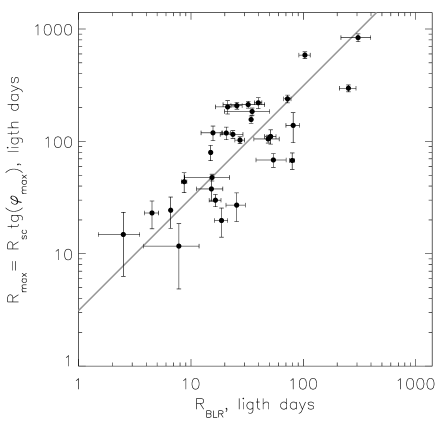
Figure 15: The maximal ($R_{max}$) vs photometric BLR ($R_{BLR}$) radius. The solid line represents the best fit.

To explain this relation, let us consider the connection between photometric size of the BLR and its real size taking photoionization as the mechanism for the broad line emission. Admitting that the reverberation gives the photometic size of the BLR, one can write:

$$R_{BLR}=c\tau\approx{\int^{R_{max}}_{R_{min}}{I(r)r}dr\over{\int^{R_{max}}_{R_{min}}{I(r)}dr}},$$

where $R_{min}$ and $R_{max}$ are the inner and outer radii of the BLR, respectively. $\tau$ is the time lag obtained from reverberation and $c$ is the light speed, and $I(r)$ is the disc emissivity. If we accept that the emissivity of the disc is $I(r)\sim r^{\alpha}$ for $\alpha\neq-1$, assuming that $R_{max}>>R_{min}$ then we have the relation between the photometric and maximum BLR radius:

$$R_{BLR}\approx{1+\alpha\over{2+\alpha}}R_{max},$$

that in the case of the flat-brightness disc ($\alpha=0$) gives $R_{BLR}=0.5R_{max}$, but if we take more realible values $\alpha=-3/4$ (Shakura and Sunyaev, 1973) the connection is $R_{BLR}=0.2R_{max}$. We obtain the relation that is between these two values, and corresponds to $\alpha\approx-0.57$, that is flatter than one expected for the classical disc emission coefficient $\alpha=-0.75$.

5 Conclusions

Here we presented results of the spectropolarimetric observations of 30 Type 1 AGNs. The measured polarization properties have been used for exploring polarization mechanisms in the continuum and determination of the BH masses and the parameters of the BLR (inclination and emissivity) using polarization in the broad H$\alpha$ line.

According to of our analysis of polarization observations of the sample of 30 broad line AGNs, we can outline following conclusions:

(i) The continuum polarization in the sample of 30 Type 1 AGNs is on the level of 1%, that is expected for this class of AGNs (see e.g. Berriman at al., 1990). The continuum polarization for all AGNs from the sample is wavelength dependent, indicating some effect of depolarization by the magnetic field or other effects. Additionally, the degree of polarization is smaller than one expected due to Thompson scattering in an accretion disc. Also the index of the polarized continuum slope is in a relatively good correlation with the black hole masses. This indicates that probably Faraday rotation has a significant role in the depolarization of the continuum light emitted from a magnetized disc.

(ii) The polarization in the H$\alpha$ broad line shows that the equatorial scattering is a dominant mechanism of polarization in the broad lines in Type 1 AGNs. The polarization angle across the broad line profile indicates dominant Keplerian-like motion in the BLR. Using the method given in Afanasiev & Popović (2015) we estimated the masses of central BHs, and found that they follow expected $M-\sigma$ relation. Also we confirmed that BH masses obtained from polarization can be used as calibration masses for other methods.

(iii) Using BH masses obtained by polarization method and corresponding ’virial products’ we estimated the BLR inclinations in our sample. We found that the most of them have the BLR inclination between 20 and 40 degrees with an average BLR inclination of $\sim$ 35 degrees.

(iv) The coefficient of BLR emissivity seems to be smaller than one expected in the Shakura-Sunyaev accretion disc ($\alpha\sim-0.75$) and the BLR tends to have a flatter emissivity ($\alpha\sim-0.57$) than the accretion disc, this should be taken into account in modelling the AGN broad line profiles.

References

- Afanasieva (2016) Afanasieva, I.V. 2016, Astrophysical Bulletin, 71, 366.
- Afanasiev & Amirkhanyan (2012) Afanasiev, V. L. & Amirkhanyan, V. R. 2012, AstBu, 67, 438.
- Afanasiev et al. (2011) Afanasiev, V. L., Borisov, N. V., Gnedin, Yu. N., et al. 2011, AstL, 37, 302
- Afanasiev & Moiseev (2011) Afanasiev, V. L., Moiseev, A. V. 2011, Baltic Astronomy, Vol. 20, p. 363
- Afanasiev & Popović (2015) Afanasiev, V. L., Popović, L. Č. 2015, ApJ, 800L, 35
- Afanasiev et al. (2014a) Afanasiev, V. L., Popović, L. Č., Shapovalova, A. I., Borisov, N. V., Ilić, D. 2014a, MNRAS, 440, 519
- Afanasiev et al. (2014b) Afanasiev, V. L., Rosenbush, V. K., Kiselev, N. N. 2014b, Astrophysical Bulletin, 69, 211
- Afanasiev et al. (2015) Afanasiev, V. L., Shapovalova, A. I., Popović, L. Č., Borisov, N. V. 2015, MNRAS, 448, 2879
- Agol & Blaes (1996) Agol, E., Blaes, O. 1996, MNRAS, 282, 965
- Agol et al. (1998) Agol, E., Blaes, O., Ionescu-Zanetti, C. 1998, MNRAS, 293, 1
- Antonucci (1993) Antonucci, R. R. J. 1993, ARA&A, 31, 473
- Antonucci & Miller (1985) Antonucci, R. R. J., Miller, J. S. 1985, ApJ, 297, 62
- Barvainis, (1987) Barvainis, R. 1987, ApJ, 320, 537
- Bentz at al. (2013) Bentz, M. C., Denney, K. D., Grier, C. J., Barth, A. J., Peterson, B. M. 2013, ApJ, 767, 149
- Bentz & Katz (2015) Bentz, M., Katz, S. 2015, PASP, 127, 67
- Bentz at al. (2009) Bentz, M., Peterson, B, M., Netzer, H, Pogge, R. W., Vestergaard, M. 2009, ApJ , 697, 160
- Berriman at al. (1990) Berriman G., Schmidt G. D., West S. C., Stockman H. S. 1990, ApJS, 74, 869
- Bon et al. (2009) Bon, E., Popović, L. Č., Gavrilović, N., La Mura, G., Mediavilla, E. 2009, MNRAS, 400, 924
- Chandrasekhar (1950) Chandrasekhar, S., 1950, Radiative Transfer (Clarendon, Oxford)
- Coatman et al. (2017) Coatman, L., Hewett, P. C., Banerji, M., Richards, G. T., Hennawi, J. F., Prochaska, J. X. 2017, MNRAS, 465, 2120
- Collin et al. (2006) Collin, S., Kawaguchi, T., Peterson, B. M., Vestergaard, M. 2006, A&A, 456, 75
- Corbett et al. (1998) Corbett, E.A. et al. 1998, MNRAS, 296, 721
- Denney et al. (2009) Denney, K. D., Watson, L. C., Peterson, B. M., Pogge, R. W., Atlee, D. W. et al. 2009, ApJ, 702, 1353
- Doroshenko et al. (2012) Doroshenko, V. T., Sergeev, S. G., Klimanov, S. A., Pronik, V. I., Efimov, Yu. S. 2012, MNRAS, 426, 416
- Eracleous & Halpern (1994) Eracleous, M., Halpern, J. P. 1994, ApJS, 90, 1
- Eracleous et al. (1996) Eracleous, M., Halpern, J. P., Livio, M. 1996, ApJ, 459, 89
- Faber & Jackson (1976) Faber, S.M., Jackson, R.E. 1976, ApJ, 204, 668
- Fausnaugh (2017) Fausnaugh, M. M. 2017, ApJ, 840, 97
- Gaskell & Goosmann (2013) Gaskell, C. M. Goosmann, R. W. 2013, ApJ, 769, 30
- Gil de Paz et al. (2007) Gil de Paz, A., Boissier, S., Madore, B. F. et al. 2007, ApJS, 173, 185
- Gnedin & Silant’ev (1997) Gnedin, Yu. N., Silant’ev, N.A. 1997, Astrophys. Space Phys., 10, 1
- Goodrich & Miller (1994) Goodrich, R.W. & Miller, J.S. 1994, ApJ, 434, 82
- Goosmann & Gaskell (2007) Goosmann, R. W., Gaskell, C. M. 2007, A&A, 465, 129
- Heisler et al. (1997) Heisler, C. A., Lumsden, S. L., & Bailey, J. A. 1997, Nature, 385, 700
- Hsu & Breger (1982) Hsu, J., Breger, M. 1982, AJ, 262, 732
- Kaspi et al. (2000) Kaspi, S., Smith, P. S., Netzer, H., Maoz, D., Jannuzi, B. T., Giveon, U. 2000, ApJ, 533, 631
- Kaspi et al. (2005) Kaspi, S., Maoz, D., Netzer, H., Peterson, B. M., Vestergaard, M., Jannuzi, B. T. 2005, ApJ, 629, 61
- Kay et al. (1999) Kay, L. et al. 1999, ASP Conference Series, 175, 205
- Kishimoto et al. (2002a) Kishimoto, M., Kay, L. E., Antonucci, R. et al. 2002a ApJ, 565, 155
- Kishimoto et al. (2002b) Kishimoto, M., Kay, L. E., Antonucci, R. at al. 2002b, ApJ, 567, 790
- Kishimoto et al. (2011) Kishimoto, M., Honig S. F., Antonucci R. et al. 2011, A&A, 527, A121
- Kollatschny (2003) Kollatschny, W. 2003, A&A, 412, L61
- Koshida at al. (2014) Koshida, S., Minezaki, T., Yoshii, Y., et al. 2014, ApJ, 788, 159
- Lumsden et al. (2004) Lumsden, S. L., Alexander, D. M., Hough, J. H. 2004, MNRAS, 348,1451
- Ma et al. (2007) Ma,R. Y., Yang, F., Wang, D. X. 2007, ApJ, 671, 1981
- Marin et al. (2012) Marin, F., Goosmann, R. W., Gaskell, C. M at al. 2012, A&A, 548, A121
- Martin et al. (1983) Martin, P.G., Tompson, I. B., Maza,J., Angel, J.R.P. 1983, ApJ, 266, 470
- Martel (1998) Martel, A. R. 1998, ApJ, 508, 657
- Mejía-Restrepo et al. (2016) Mejía-Restrepo, J. E., Trakhtenbrot, B., Lira, P., Netzer, H., Capellupo, D. M. 2016, MNRAS, 460, 187
- Miller & Goodrich (1990) Miller, J. S., Goodrich, R. W. 1990, ApJ, 355, 456
- Moran et al. (2000) Moran, E. C., Barth, A. J., Kay, L. E., Filippenko, A. V., 2000, ApJ, 540L, 73
- Oliva (1997) Oliva, E. 1997, A&AS, 123, 589
- Onken & Kollmeie (2008) Onken, C. A. & Kollmeier, J. A. 2008, ApJ, 689L, 13
- Onken et al. (2004) Onken, C. A., Ferrarese, L., Merritt, D., et al. 2004, ApJ, 615, 645
- Peterson (2014) Peterson, B. M. 2014, SSRev, 183, 253
- Peterson et al. (2004) Peterson, B. M., Ferrarese, L., Gilbert, K. M., Kaspi, S., Malkan, M. A. et al. 2004, ApJ, 613, 682
- Popović et al. (2004) Popović, L. Č., Mediavilla, E., Bon, E., & Ilić, D. 2004, A&A, 423, 909
- Ramos Almeida et al. (2016) Ramos Almeida, C., Martínez González, M. J., Asensio Ramos, A., Acosta-Pulido, J. A., et al., 2016, MNRAS, 461, 1387
- Savić et al. (2018) Savić, D., Goosmann, R., Popović, L.Č., Marin, F., Afanasiev, V. L. 2018, A&A, 614A, 120.
- Schmidt et al. (1992) Schmidt, G.D., Elston, R. and Lupie, O.L., 1992, AJ, 104, 1563
- Schmidt & Miller (1985) Schmidt, G.D. Miller, J.S. 1985, ApJ, 290, 517
- Shakura and Sunyaev (1973) Shakura, N. I., Sunyaev, R. A. 1973, A&A, 24, 337S
- Serkowski et al. (1975) Serkowski K., Mthewson D. S., Ford V. L. 1975, ApJ, 196, 261
- Simmons and Stewart (1985) Simmons, J.F.L. and Stewart, B.G., 1985, A&A, 142, 100
- Smith et al. (2004) Smith, J. E., Robinson, A., Alexander, D. M., et al. 2004, MNRAS, 350, 140
- Smith et al. (2005) Smith, J. E., Robinson, A., Young, S., et al. 2005, MNRAS, 359, 846
- Smith et al. (2002) Smith, J. E., Young, S., Robinson, A., et al. 2002, MNRAS, 335, 773
- Storchi-Bergmann et al. (2017) Storchi-Bergmann, T., Schimoia, J. S., Peterson, B. M., Elvis, M., Denney, K. D., Eracleous, M., Nemmen, R. S. 2017, ApJ, 835, 236
- Tilton & Shull (2013) Tilton, E. M., Shull, J. M. 2013, ApJ, 774, 67
- Trakhtenbrot & Netzer (2012) Trakhtenbrot, B., Netzer, H. 2012, MNRAS, 427, 3081
- Tran (2001) Tran, H. D. 2001, ApJ, 554, L19
- Tran (2003) Tran, H. T., 2003, NewAR, 47, 1091
- Tran et al. (1992) Tran, H. D., Miller, J. S., & Kay, L. E. 1992, ApJ, 397, 452
- Tremaine et al (2002) Tremaine, S. Gebhardt, K., Bender, R., Bower, G., Dressler, A. et al. 2002, ApJ, 574, 740
- Turnshek et al. (1990) Turnshek, D.A., Bohlin, R. C., Williamson, R. L., II, Lupie, O. L., Koornneef, J., Morgan, D. H. 1990, AJ. 99, 1243
- Vestergaard (2002) Vestergaard, M. 2002, ApJ, 571, 733
- Vestergaard & Peterson (2006) Vestergaard, M., Peterson, B. M. 2006, ApJ, 641, 689
- Wang et al. (2009) Wang, J.-G., Dong, X.-B., Wang, T.-G., Ho, L. C., Yuan, W., Wang, H., Zhang, K., Zhang, S., Zhou, H. 2009, ApJ, 707, 1334
- Wills et al. (1992a) Wills, B.J. et al. 1992a, ApJ, 398, 454
- Wills et al. (1992b) Wills, B.J. et al. 1992b, ApJ, 400, 96 bibitem[Wolf & Henning(1999)]wo99 Wolf, S., Henning, Th. 1999, A&A, 341, 675
- Young et al. (1996) Young, S., Hough, J. H., Axon, D. J.et al. 1996, MNRAS, 280, 291
- Zu et al. (2011) Zu, Y., Kochanek, C. S., Peterson, B. M. 2011, ApJ, 735, 80