On Controllable Sparse Alternatives to Softmax

Abstract

Converting an n-dimensional vector to a probability distribution over n objects is a commonly used component in many machine learning tasks like multiclass classification, multilabel classification, attention mechanisms etc. For this, several probability mapping functions have been proposed and employed in literature such as softmax, sum-normalization, spherical softmax, and sparsemax, but there is very little understanding in terms how they relate with each other. Further, none of the above formulations offer an explicit control over the degree of sparsity. To address this, we develop a unified framework that encompasses all these formulations as special cases. This framework ensures simple closed-form solutions and existence of sub-gradients suitable for learning via backpropagation. Within this framework, we propose two novel sparse formulations, sparsegen-lin and sparsehourglass, that seek to provide a control over the degree of desired sparsity. We further develop novel convex loss functions that help induce the behavior of aforementioned formulations in the multilabel classification setting, showing improved performance. We also demonstrate empirically that the proposed formulations, when used to compute attention weights, achieve better or comparable performance on standard seq2seq tasks like neural machine translation and abstractive summarization.

1 Introduction

Various widely used probability mapping functions such as sum-normalization, softmax, and spherical softmax enable mapping of vectors from the euclidean space to probability distributions. The need for such functions arises in multiple problem settings like multiclass classification [1, 2], reinforcement learning [3, 4] and more recently in attention mechanism [5, 6, 7, 8, 9] in deep neural networks, amongst others. Even though softmax is the most prevalent approach amongst them, it has a shortcoming in that its outputs are composed of only non-zeroes and is therefore ill-suited for producing sparse probability distributions as output. The need for sparsity is motivated by parsimonious representations [10] investigated in the context of variable or feature selection. Sparsity in the input space offers benefits of model interpretability as well as computational benefits whereas on the output side, it helps in filtering large output spaces, for example in large scale multilabel classification settings [11]. While there have been several such mapping functions proposed in literature such as softmax [4], spherical softmax [12, 13] and sparsemax [14, 15], very little is understood in terms of how they relate to each other and their theoretical underpinnings. Further, for sparse formulations, often there is a need to trade-off interpretability for accuracy, yet none of these formulations offer an explicit control over the desired degree of sparsity.

Motivated by these shortcomings, in this paper, we introduce a general formulation encompassing all such probability mapping functions which serves as a unifying framework to understand individual formulations such as hardmax, softmax, sum-normalization, spherical softmax and sparsemax as special cases, while at the same time helps in providing explicit control over degree of sparsity. With the aim of controlling sparsity, we propose two new formulations: sparsegen-lin and sparsehourglass. Our framework also ensures simple closed-form solutions and existence of sub-gradients similar to softmax. This enables them to be employed as activation functions in neural networks which require gradients for backpropagation and are suitable for tasks that require sparse attention mechanism [14]. We also show that the sparsehourglass formulation can extend from translation invariance to scale invariance with an explicit control, thus helping to achieve an adaptive trade-off between these invariance properties as may be required in a problem domain.

We further propose new convex loss functions which can help induce the behaviour of the above proposed formulations in a multilabel classification setting. These loss functions are derived from a violation of constraints required to be satisfied by the corresponding mapping functions. This way of defining losses leads to an alternative loss definition for even the sparsemax function [14]. Through experiments we are able to achieve improved results in terms of sparsity and prediction accuracies for multilabel classification.

Lastly, the existence of sub-gradients for our proposed formulations enable us to employ them to compute attention weights [5, 7] in natural language generation tasks. The explicit controls provided by sparsegen-lin and sparsehourglass help to achieve higher interpretability while providing better or comparable accuracy scores. A recent work [16] had also proposed a framework for attention; however, they had not explored the effect of explicit sparsity controls. To summarize, our contributions are the following:

• A general framework of formulations producing probability distributions with connections to hardmax, softmax, sparsemax, spherical softmax and sum-normalization (Sec.3).

• New formulations like sparsegen-lin and sparsehourglass as special cases of the general framework which enable explicit control over the desired degree of sparsity (Sec.3.2,3.5).

• A formulation sparsehourglass which enables us to adaptively trade-off between the translation and scale invariance properties through explicit control (Sec.3.5).

• Convex multilabel loss functions correponding to all the above formulations proposed by us. This enable us to achieve improvements in the multilabel classification problem (Sec.4).

• Experiments for sparse attention on natural language generation tasks showing comparable or better accuracy scores while achieving higher interpretability (Sec.5).

2 Preliminaries and Problem Setup

Notations: For $K\in\mathbb{Z}_{+}$, we denote $[K]:=\{1,\ldots,K\}$. Let $\bm{z}\in\mathbb{R}^{K}$ be a real vector denoted as $\bm{z}=\{z_{1},\ldots,z_{K}\}$. 1 and 0 denote vector of ones and zeros resp. Let $\Delta^{K-1}:=\{\bm{p}\in\mathbb{R}^{K}\ |\ \textbf{1}^{T}\bm{p}=1,\bm{p}\geq\textbf{0}\}$ be the $(K-1)$-dimensional simplex and $\bm{p}\in\Delta^{K-1}$ be denoted as $\bm{p}=\{p_{1},\ldots,p_{K}\}$. We use $[t]_{+}:=\text{max}\{0,t\}$. Let $A(\bm{z}):=\{k\in[K]\ |\ z_{k}=\max_{j}z_{j}\}$ be the set of maximal elements of $z$.

Definition: A probability mapping function is a map $\rho:\mathbb{R}^{K}\rightarrow\Delta^{K-1}$ which transforms a score vector $\bm{z}$ to a categorical distribution (denoted as $\rho(\bm{z})=\{\rho_{1}(\bm{z}),\ldots,\rho_{K}(\bm{z})\}$). The support of $\rho(\bm{z})$ is $S(\bm{z}):=\{j\in[K]\ |\ \rho_{j}(\bm{z})>0\}$. Such mapping functions can be used as activation function for machine learning models. Some known probability mapping functions are listed below:

• Softmax function is defined as: $\rho_{i}(\bm{z})=\frac{\text{exp}(z_{i})}{\sum_{j\in[K]}\text{exp}(z_{j})},\ \forall i\in[K].$ Softmax is easy to evaluate and differentiate and its logarithm is the negative log-likelihood loss [14].

• Spherical softmax - Another function which is simple to compute and derivative-friendly: $\rho_{i}(\bm{z})=\frac{z_{i}^{2}}{\sum_{j\in[K]}z_{j}^{2}},\ \forall i\in[K].$ Spherical softmax is not defined for $\sum_{j\in[K]}z_{j}^{2}=0$.

• Sum-normalization : $\rho_{i}(\bm{z})=\frac{z_{i}}{\sum_{j\in[K]}z_{j}},\ \forall i\in[K].$ It is not used in practice much as the mapping is not defined if $z_{i}<0$ for any $i\in[K]$ and for $\sum_{j\in[K]}z_{j}=0$.

The above mapping functions are limited to producing distributions with full support. Consider there is a single value of $z_{i}$ significantly higher than the rest, its desired probability should be exactly 1, while the rest should be grounded to zero (hardmax mapping). Unfortunately, that does not happen unless the rest of the values tend to $-\infty$ (in case of softmax) or are equal to $0$ (in case of spherical softmax and sum-normalization).

• Sparsemax recently introduced by [14] circumvents this issue by projecting the score vector $\bm{z}$ onto a simplex [15]: $\rho(\bm{z})=\operatorname*{argmin}_{\bm{p}\in\Delta^{K-1}}\|\bm{p}-\bm{z}\|^{2}_{2}$. This offers an intermediate solution between softmax (no zeroes) and hardmax (zeroes except for the highest value).

(a) Softmax

(b) Sparsemax

(c) Sum-normalization

Figure 1: Visualization of probability mapping functions in two-dimension. The contour plots show values of $\rho_{1}(\bm{z})$. The green line segment connecting (1,0) and (0,1) is the 1-dimensional probability simplex. Each contour (here it is line) contains points in $\mathbb{R}^{2}$ plane which have the same $\rho_{1}(\bm{z})$, the exact value marked on the contour line.

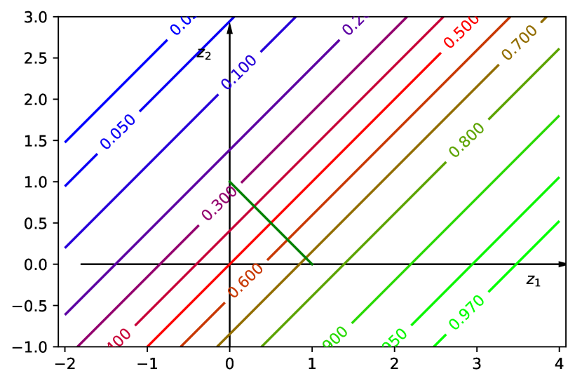
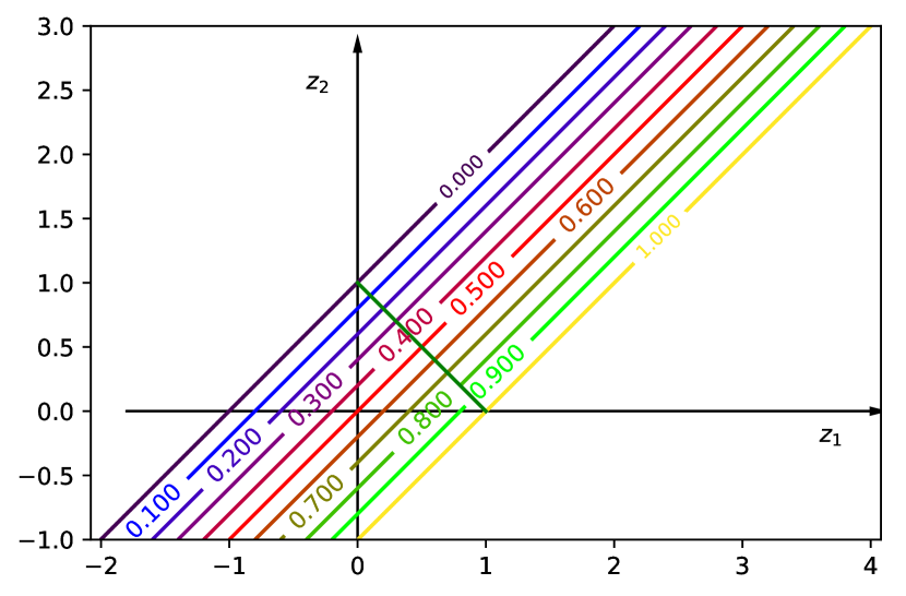
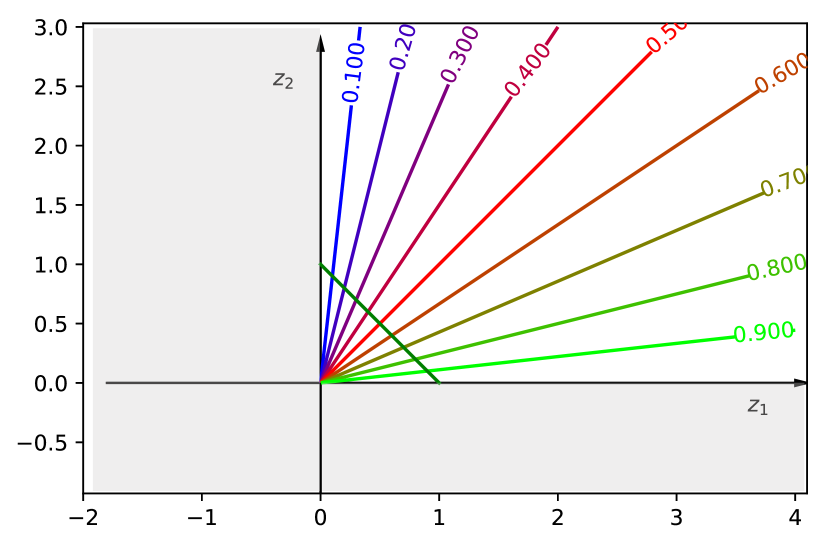
The contour plots for softmax, sparsemax and sum-normalization in two-dimensions ($\bm{z}\in\mathbb{R}^{2}$) are shown in Fig.1. The contours of sparsemax are concentrated over a narrow region, while the remaining region corresponds to sparse solutions. For softmax, the contour plots are spread over the whole real plane, confirming the absence of sparse solutions. Sum-normalization is not defined outside the first quadrant, and yet, the contours cover the whole quadrant, denying sparse solutions.

3 Sparsegen Activation Framework

Definition: We propose a generic probability mapping function inspired from the sparsemax formulation (in Sec.2) which we call sparsegen:

$$\rho(\bm{z})=\text{sparsegen}(\bm{z};g,\lambda)=\operatorname*{argmin}_{\bm{p}\in\Delta^{K-1}}\ \ \|\bm{p}-g(\bm{z})\|^{2}_{2}-\lambda\|\bm{p}\|^{2}_{2}$$ (1)

where $g:\mathbb{R}^{K}\rightarrow\mathbb{R}^{K}$ is a component-wise transformation function applied on $\bm{z}$. Here $g_{i}(\bm{z})$ denotes the $i$-th component of $g(\bm{z})$. The coefficient $\lambda<1$ controls the regularization strength. For $\lambda>0$, the second term becomes negative $L$-2 norm of $\bm{p}$. In addition to minimizing the error on projection of $g(\bm{z})$, Eq.1 tries to maximize the norm, which encourages larger probability values for some indices, hence moving the rest to zero. The above formulation has a closed-form solution (see App. A.1 for solution details), which can be computed in $O(K)$ time using the modified randomized median finding algorithm as followed in [15] while solving the projection onto simplex problem.

The choices of both $\lambda$ and $g$ can help control the cardinality of the support set $S(\bm{z})$, thus influencing the sparsity of $\rho(\bm{z})$. $\lambda$ can help produce distributions with support ranging from full (uniform distribution when $\lambda\rightarrow 1^{-}$) to minimum (hardmax when $\lambda\rightarrow-\infty$). Let $S(\bm{z},\lambda_{1})$ denote the support of sparsegen for a particular coefficient $\lambda_{1}$. It is easy to show: if $|S(\bm{z},\lambda_{1})|>|A(\bm{z})|$, then there exists $\lambda_{x}>\lambda_{1}$ for an $x<|S(\bm{z},\lambda_{1})|$ such that $|S(\bm{z},\lambda_{x})|=x$. In other words, if a sparser solution exists, it can be obtained by changing $\lambda$. The following result has an alternate interpretation for $\lambda$:

Result: The sparsegen formulation (Eq.1) is equivalent to the following, when $\gamma=\frac{1}{1-\lambda}$ (where $\gamma>0$): $\rho(\bm{z})=\operatorname*{argmin}_{\bm{p}\in\Delta^{K-1}}\|\bm{p}-\gamma g(\bm{z})\|^{2}_{2}$.

The above result says that scaling $g(\bm{z})$ by $\gamma=\frac{1}{1-\lambda}$ is equivalent to applying the negative $L$-2 norm with $\lambda$ coefficient when considering projection of $g(\bm{z})$ onto the simplex. Thus, we can write:

$$\text{sparsegen}(\bm{z};g,\lambda)=\text{sparsemax}\Big{(}\frac{g(\bm{z})}{1-\lambda}\Big{)}.$$ (2)

This equivalence helps us borrow results from sparsemax to establish various properties for sparsegen.

Jacobian of sparsegen: To train a model with sparsegen as an activation function, it is essential to compute its Jacobian matrix denoted by $J_{\rho}(\bm{z}):=[\partial\rho_{i}(\bm{z})/\partial z_{j}]_{i,j}$ for using gradient-based optimization techniques. We use Eq.2 and results from [14](Sec.2.5) to derive the Jacobian for sparsegen by applying chain rule of derivatives:

$$J_{\text{sparsegen}}(\bm{z})=J_{\text{sparsemax}}\Big{(}\frac{g(\bm{z})}{1-\lambda}\Big{)}\times\frac{J_{g}(\bm{z})}{1-\lambda}$$ (3)

where $J_{g}(\bm{z})$ is Jacobian of $g(\bm{z})$ and $J_{\text{sparsemax}}(\bm{z})=\Big{[}\text{Diag}(\bm{s})-\frac{\bm{s}\bm{s}^{T}}{|S(\bm{z})|}\Big{]}$. Here $\bm{s}$ is an indicator vector whose $i^{\text{th}}$ entry is 1 if $i\in S(\bm{z})$. $\text{Diag}(\bm{s})$ is a matrix created using $\bm{s}$ as its diagonal entries.

3.1 Special cases of Sparsegen: sparsemax, softmax and spherical softmax

Apart from $\lambda$, one can control the sparsity of sparsegen through $g(\bm{z})$ as well. Moreover, certain choices of $\lambda$ and $g(\bm{z})$ help us establish connections with existing activation functions (see Sec.2). The following cases illustrate these connections (more details in App.A.2):

Example 1: $\bm{g(z)=\text{exp}(z)}$ (sparsegen-exp): $\text{exp}(\bm{z})$ denotes element-wise exponentiation of $\bm{z}$, that is $g_{i}(\bm{z})=\text{exp}(z_{i})$. Sparsegen-exp reduces to softmax when $\lambda=1-\sum_{j\in[K]}e^{z_{j}}$, as it results in $S(\bm{z})=[K]$ as per Eq.13 in App.A.2.

Example 2: $\bm{g(z)=z^{2}}$ (sparsegen-sq): $\bm{z}^{2}$ denotes element-wise square of $\bm{z}$. As observed for sparsegen-exp, when $\lambda=1-\sum_{j\in[K]}z^{2}_{j}$, sparsegen-sq reduces to spherical softmax.

Example 3 : $\bm{g(\bm{z})=\bm{z}},\bm{\lambda}=0$: This case is equivalent to the projection onto the simplex objective adopted by sparsemax. Setting $\lambda\neq 0$ leads the regularized extension of sparsemax as seen next.

3.2 Sparsegen-lin: Extension of sparsemax

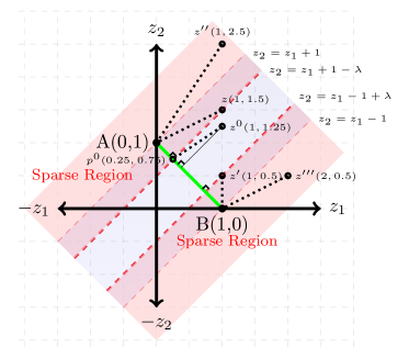
The negative $L$-2 norm regularizer in Eq.4 helps to control the width of the non-sparse region (see Fig.2 for the region plot in two-dimensions). In the extreme case of $\lambda\rightarrow 1^{-}$, the whole real plane maps to sparse region whereas for $\lambda\rightarrow-\infty$, the whole real plane renders non-sparse solutions.

$$\rho(\bm{z})=\text{sparsegen-lin}(\bm{z})=\operatorname*{argmin}_{\bm{p}\in\Delta^{K-1}}\ \ \|\bm{p}-\bm{z}\|^{2}_{2}-\lambda\|\bm{p}\|^{2}_{2}$$ (4)

[capbesideposition=right,bottom,capbesidewidth=7cm]figure[]

Figure 2: Sparsegen-lin: Region plot for $\bm{z}=\{z_{1},z_{2}\}\in\mathbb{R}^{2}$ when $\lambda=0.5$. $\rho(\bm{z})$ is sparse in the red region, whereas non-sparse in the blue region. The dashed red lines depict the boundaries between sparse and non-sparse regions. For $\lambda=0.5$, points like ($\bm{z}$ or $\bm{z}^{\prime}$) are mapped onto the sparse points A or B. Whereas for sparsemax ($\lambda=0$), they fall in the blue region (the boundaries of sparsemax are shown by lighter dashed red lines passing through A and B). The point $\bm{z}^{0}$ lies in the blue region, producing non-sparse solution. Interestingly more points like $\bm{z^{\prime\prime}}$ and $\bm{z^{\prime\prime\prime}}$, which currently lie in the red region can fall in the blue region for some $\lambda<0$. For $\lambda>0.5$, the blue region becomes smaller, as mores points map to sparse solutions.

3.3 Desirable properties for probability mapping functions

Let us enumerate below some properties a probability mapping function $\rho$ should possess:

1. Monotonicity: If $z_{i}\geq z_{j}$, then $\rho_{i}(\bm{z})\geq\rho_{j}(\bm{z})$. This does not always hold true for sum-normalization and spherical softmax when one or both of $z_{i},z_{j}$ is less than zero. For sparsegen, both $g_{i}(\bm{z})$ and $g_{i}(\bm{z})/(1-\lambda)$ should be monotonic increasing, which implies $\lambda$ needs to be less than 1.

2. Full domain: The domain of $\rho$ should include negatives as well as positives, i.e. $\text{Dom}(\rho)\in\mathbb{R}^{K}$. Sum-normalization does not satisfy this as it is not defined if some dimensions of $\bm{z}$ are negative.

3. Existence of Jacobian: This enables usage in any training algorithm where gradient-based optimization is used. For sparsegen, the Jacobian of $g(\bm{z})$ should be easily computable (Eq.3).

4. Lipschitz continuity: The derivative of the function should be upper bounded. This is important for the stability of optimization technique used in training. Softmax and sparsemax are 1-Lipschitz whereas spherical softmax and sum-normalization are not Lipschitz continuous. Eq.3 shows the Lipschitz constant for sparsegen is upper bounded by $1/(1-\lambda)$ times the Lipschitz constant for $g(\bm{z})$.

5. Translation invariance: Adding a constant $c$ to every element in $\bm{z}$ should not change the output distribution : $\rho(\bm{z}+c\bm{1})=\rho(\bm{z})$. Sparsemax and softmax are translation invariant whereas sum-normalization and spherical softmax are not. Sparsegen is translation invariant iff for all $c\in\mathbb{R}$ there exist a $\tilde{c}\in\mathbb{R}$ such that $g(\bm{z}+c\bm{1})=g(\bm{z})+\tilde{c}\bm{1}$. This follows from Eq.2.

6. Scale invariance: Multiplying every element in $\bm{z}$ by a constant $c$ should not change the output distribution : $\rho(c\bm{z})=\rho(\bm{z})$. Sum-normalization and spherical softmax satisfy this property whereas sparsemax and softmax are not scale invariant. Sparsegen is scale invariant iff for all $c\in\mathbb{R}$ there exist a $\hat{c}\in\mathbb{R}$ such that $g(c\bm{z})=g(\bm{z})+\hat{c}\bm{1}$. This also follows from Eq.2.

7. Permutation invariance: If there is a permutation matrix $\bm{P}$, then $\rho(\bm{P}\bm{z})=\bm{P}\rho(\bm{z})$. For sparsegen, the precondition is that $g(\bm{z})$ should be a permutation invariant function.

8. Idempotence: $\rho(\bm{z})=\bm{z}$, $\forall\bm{z}\in\Delta^{K-1}$. This is true for sparsemax and sum-normalization. For sparsegen, it is true if and only if $g(\bm{z})=\bm{z},\ \forall\bm{z}\in\Delta^{K-1}$ and $\lambda=0$.

In the next section, we discuss in detail about the scale invariance and translation invariance properties and propose a new formulation achieving a trade-off between these properties.

3.4 Trading off Translation and Scale Invariances

As mentioned in Sec.1, scale invariance is a desirable property to have for probability mapping functions. Consider applying sparsemax on two vectors $\bm{z}=\{0,1\}$, $\bm{\bar{z}}=\{100,101\}\in\mathbb{R}^{2}$. Both would result in $\{0,1\}$ as the output. However, ideally $\bm{\bar{z}}$ should have mapped to a distribution nearer to $\{0.5,0.5\}$ instead. Scale invariant functions will not have such a problem. Among the existing functions, only sum-normalization and spherical softmax satisfy scale invariance. While sum-normalization is only defined for positive values of $\bm{z}$, spherical softmax is not monotonic or Lipschitz continuous. In addition, both of these methods are also not defined for $\bm{z}=\bm{0}$, thus making them unusable for practical purposes. It can be shown that any probability mapping function with the scale invariance property will not be Lipschitz continuous and will be undefined for $\bm{z}=\bm{0}$.

A recent work[13] had pointed out the lack of clarity over whether scale invariance is more desired than the translation invariance property of softmax and sparsemax. We take this into account to achieve trade-off between the two invariances. In the usual scale invariance property, scaling vector $\bm{z}$ essentially results in another vector along the line connecting $\bm{z}$ and the origin. That resultant vector also has the same output probability distribution as the original vector (See Sec. 3.3). We propose to scale the vector $\bm{z}$ along the line connecting it with a point (we call it anchor point henceforth) other than the origin, yet achieving the same output. Interestingly, the choice of this anchor point can act as a control to help achieve a trade-off between scale invariance and translation invariance.

Let a vector $\bm{z}$ be projected onto the simplex along the line connecting it with an anchor point $\bm{q}=(-q,\dots,-q)\in\mathbb{R}^{K}$, for $q>0$ (See Fig.3a for $K=2$). We choose $g(\bm{z})$ as the point where this line intersects with the affine hyperplane $\bm{1}^{T}\bm{\hat{z}}=1$ containing the probability simplex. Thus, $g(\bm{z})$ is set equal to $\alpha\bm{z}+(1-\alpha)\bm{q}$, where $\alpha=\frac{1+Kq}{\sum_{i}z_{i}+Kq}$ (we denote it as $\alpha(\bm{z})$ as $\alpha$ is a function of $\bm{z}$). From the translation invariance property of sparsemax, the resultant mapping function can be shown equivalent to considering $g(\bm{z})=\alpha(\bm{z})\bm{z}$ in Eq.1. We refer to this variant of sparsegen assuming $g(\bm{z})=\alpha(\bm{z})\bm{z}$ and $\lambda=0$ as sparsecone.

(a) Sparsecone

(b) Sparsehourglass

Figure 3: (a) Sparsecone: The vector $\bm{z}$ maps to a point $\bm{p}$ on the simplex along the line connecting to the point $\bm{q}=(-q,-q)$. Here we consider $q=1$. The red region corresponds to sparse region whereas blue covers the non-sparse region. (b) Sparsehourglass: For the vector $\bm{z}^{\prime}$ in the positive half-space, the mapping to the solution $\bm{p}^{\prime}$ can be obtained similarly as sparsecone. For the vector $\bm{z}$ in the negative half-space, a mirror point $\tilde{\bm{z}}$ needs to be found, which leads to the solution $\bm{p}$.

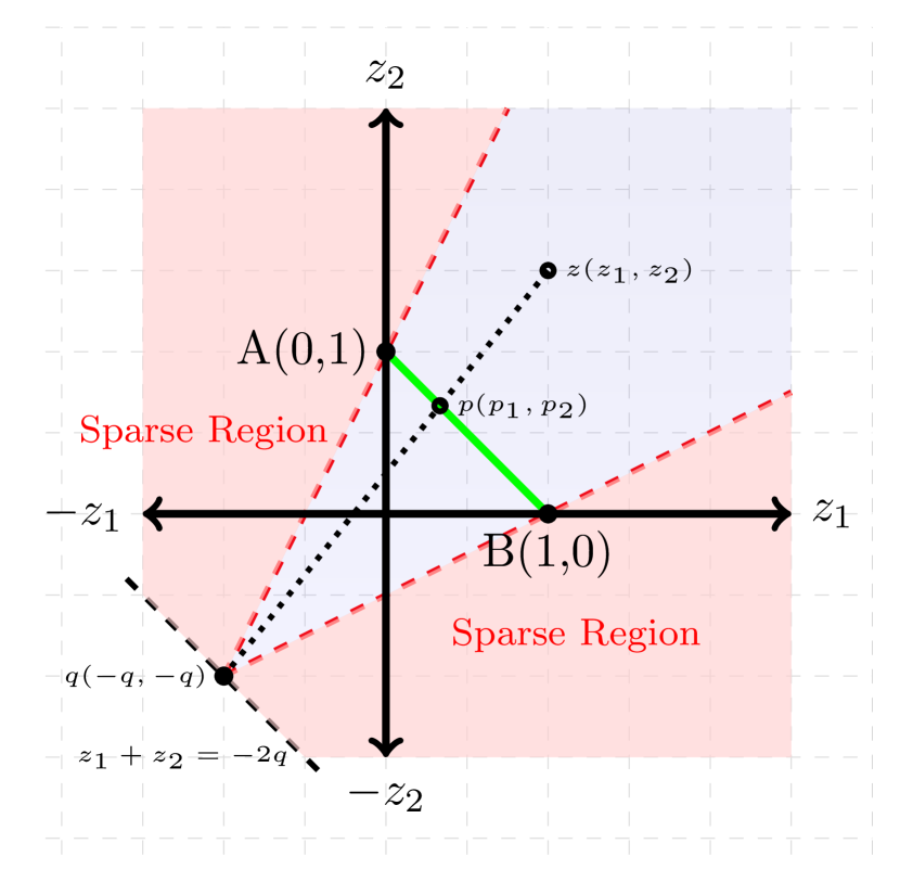
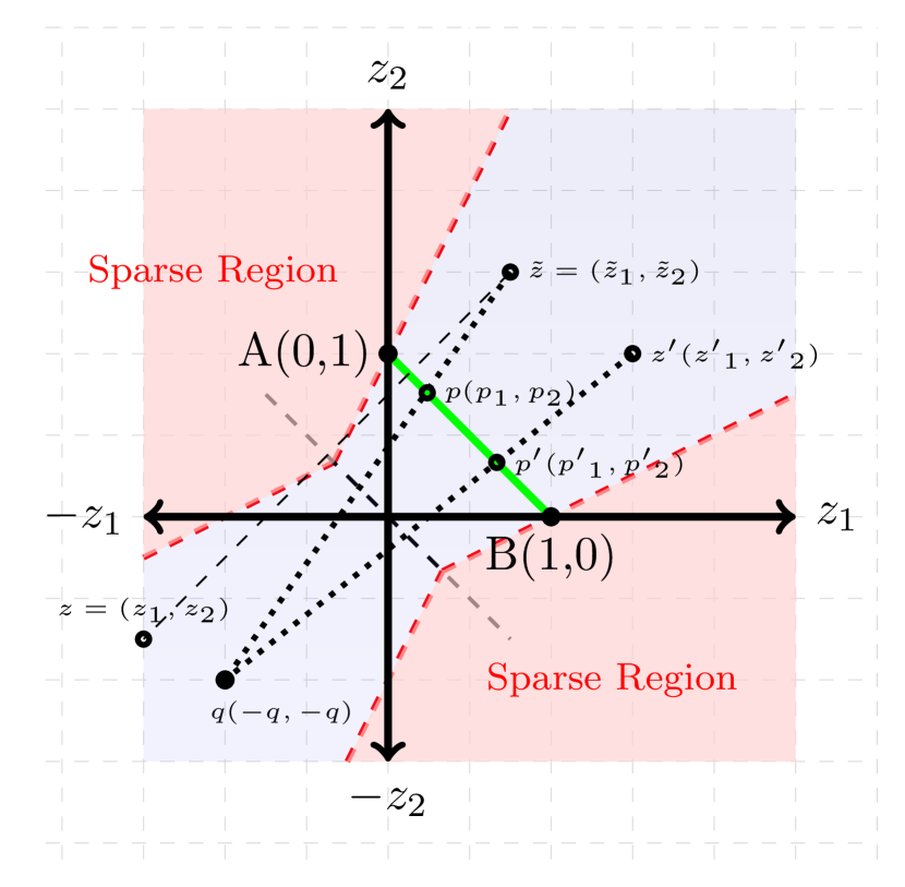
Interestingly, when the parameter $q=0$, sparsecone reduces to sum-normalization (scale invariant) and when $q\rightarrow\infty$, it is equivalent to sparsemax (translation invariant). Thus the parameter $q$ acts as a control taking sparsecone from scale invariance to translation invariance. At intermediate values (that is, for $0<q<\infty$), sparsecone is approximate scale invariant with respect to the anchor point $\bm{q}$. However, it is undefined for $\bm{z}$ where $\sum_{i}z_{i}<-Kq$ (beyond the black dashed line shown in Fig.3a). In this case the denominator term of $\alpha(\bm{z})$ (that is, $\sum_{i}z_{i}+Kq$) becomes negative destroying the monotonicity of $\alpha(\bm{z})\bm{z}$. Also note that sparsecone is not Lipschitz continuous.

3.5 Proposed Solution: Sparsehourglass

To alleviate the issue of monotonicity when $\sum_{i}z_{i}<-Kq$, we choose to restrict applying sparsecone only for the positive half-space $\mathbb{H}^{K}_{+}:=\{\bm{z}\in\mathbb{R}^{K}\ |\ \sum_{i}z_{i}\geq 0\}$. For the remaining negative half-space $\mathbb{H}^{K}_{-}:=\{\bm{z}\in\mathbb{R}^{K}\ |\ \sum_{i}z_{i}<0\}$, we define a mirror point function to transform to a point in $\mathbb{H}^{K}_{+}$, on which sparsecone can be applied. Thus the solution for a point in the negative half-space is given by the solution of its corresponding mirror point in the positive half-space. This mirror point function has some necessary properties (see App. A.4 for details), which can be satisfied by defining $m$: $m_{i}(\bm{z})=z_{i}-\frac{2\sum_{j}z_{j}}{K},\ \forall i\in[K]$. Interestingly, this can alternatively be achieved by choosing $g(\bm{z})=\hat{\alpha}(\bm{z})\bm{z}$, where $\hat{\alpha}$ is a slight modification of $\alpha$ given by $\hat{\alpha}(\bm{z})=\frac{1+Kq}{|\sum_{i}z_{i}|+Kq}$. This leads to the definition of a new probability mapping function (which we call sparsehourglass):

$$\rho(\bm{z})=\text{sparsehourglass}(\bm{z})=\operatorname*{argmin}_{\bm{p}\in\Delta^{K-1}}\Big{\|}\bm{p}-\frac{1+Kq}{|\sum_{i\in[K]}z_{i}|+Kq}\bm{z}\Big{\|}^{2}_{2}$$ (5)

Like sparsecone, sparsehourglass also reduces to sparsemax when $q\rightarrow\infty$. Similarly, $q=0$ for sparsehourglass leads to a corrected version of sum-normalization (we call it sum normalization++ ), which works for the negative domain as well unlike the original version defined in Sec.2. Another advantage of sparsehourglass is that it is Lipschitz continuous with Lipschitz constant equal to $(1+\frac{1}{Kq})$ (proof details in App.A.5). Table.1 summarizes all the formulations seen in this paper and compares them against the various important properties mentioned in Sec.3.3. Note that sparsehourglass is the only probability mapping function which satisfies all the properties. Even though it does not satisfy both scale invariance and translation invariance simultaneously, it is possible to achieve these separately through different values of $q$ parameter, which can be decided independent of $\bm{z}$.

Function	Idempotence	Monotonic	Translation Inv	Scale Inv	Full Domain	Lipschitz
Sum Normalization	✔	✗	✗	✔	✗	$\infty$
Spherical Softmax	✗	✗	✗	✔	✗	$\infty$
Softmax	✗	✔	✔	✗	✔	1
Sparsemax	✔	✔	✔	✗	✔	1
Sparsegen-lin	✓	✔	✔	✗	✔	$1/(1-\lambda)$
Sparsegen-exp	✗	✔	✗	✗	✔	$\infty$
Sparsegen-sq	✗	✗	✗	✗	✔	$\infty$
Sparsecone	✔	✗	✓	✓	✗	$\infty$
Sparsehourglass	✔	✔	✓	✓	✔	$(1+1/Kq)$
Sum Normalization++	✔	✔	✗	✔	✔	$\infty$

Table 1: Summary of the properties satisfied by probability mapping functions. Here ✔ denotes ‘satisfied in general’, ✗ signifies ‘not satisfied’ and ✓says ‘satisfied for some constant parameter independent of $\bm{z}$’. Note that Permutation Inv and existence of Jacobian are satisfied by all.

4 Sparsity Inducing Loss Functions for Multilabel Classification

An important usage of such sparse probability mapping functions is in the output mapping of multilabel classification models. Typical multilabel problems have hundreds of possible labels or tags, but any single instance has only a few tags [17]. Thus, a function which takes in a vector in $\mathbb{R}^{K}$ and outputs a sparse version of the vector is of great value.

Given training instances $(\bm{x}_{i},\bm{y}_{i})\in\pazocal{X}\times\{0,1\}^{K}$, we need to find a model function $f:\pazocal{X}\rightarrow\mathbb{R}^{K}$ that produces score vector over the label space, which on application of $\rho:\mathbb{R}^{K}\rightarrow\Delta^{K-1}$ (the sparse probability mapping function in question) leads to correct prediction of label vector $\bm{y}_{i}$. Define $\bm{\eta}_{i}:=\bm{y}_{i}/\|\bm{y}_{i}\|_{1}$, which is a probability distribution over the labels. Considering a loss function $\mathscr{L}:\Delta^{K-1}\times\Delta^{K-1}\rightarrow[0,\infty)$ and representing $\bm{z}_{i}:=f(\bm{x}_{i})$, a natural way for training using $\rho$ is to find a function $f:\pazocal{X}\rightarrow\mathbb{R}^{K}$ that minimises the error $R(f)$ below over a hypothesis class $\pazocal{F}$:

$$R(f)=\sum_{i=1}^{M}\mathscr{L}(\rho(\bm{z}_{i}),\bm{\eta}_{i})$$

In the prediction phase, for a test instance $\bm{x}$, one can simply predict the non-zero elements in the vector $\rho(f^{*}(\bm{x}))$ where $f^{*}$ is the minimizer of the above training objective $R(f)$.

For all cases where $\rho$ produces sparse probability distributions, one can show that the training objective $R$ above is highly non-convex in $f$, even for the case of a linear hypothesis class $\pazocal{F}$. However, when we remove the requirement of $\rho(\bm{z})$ being there in training part, and use a loss function which works with $\bm{z}$ and $\bm{y}$, we can obtain a system which is convex in $f$. We, thus, design a loss function $\pazocal{L}:\mathbb{R}^{K}\times\Delta^{K-1}\rightarrow[0,\infty)$ such that $\pazocal{L}(\bm{z},\bm{\eta})=0$ only if $\rho(\bm{z})=\bm{\eta}$. To derive such a loss function, we proceed by enumerating a list of constraints which will be satisfied by the zero-loss region in the $K$-dimensional space of the vector $\bm{z}$. For sparsehourglass, the closed-form solution is given by $\rho_{i}(\bm{z})=[\hat{\alpha}(\bm{z})z_{i}-\tau(\bm{z})]_{+}$ (see App.A.1). This enables us to list down the following constraints for zero loss: (1) $\hat{\alpha}(\bm{z})(z_{i}-z_{j})=0,\ \forall i,j\ |\eta_{i}=\eta_{j}\neq 0$, and (2) $\hat{\alpha}(\bm{z})(z_{i}-z_{j})\geq\eta_{i},\ \forall i,j\ |\eta_{i}\neq 0,\eta_{j}=0$. The value of the loss when any such constraints is violated is simply determined by piece-wise linear functions, which lead to the following loss function for sparsehourglass:

$$\begin{split}\pazocal{L}_{\text{sparsehg,hinge}}(\bm{z},\bm{\eta})&=\sum\limits_{\begin{subarray}{c}i,j\\ \eta_{i}\neq 0,\eta_{j}\neq 0\end{subarray}}\big{|}z_{i}-z_{j}\big{|}+\sum\limits_{\begin{subarray}{c}i,j\\ \eta_{i}\neq 0,\eta_{j}=0\end{subarray}}\text{max}\Big{\{}\frac{\eta_{i}}{\hat{\alpha}(\bm{z})}-(z_{i}-z_{j}),0\Big{\}}.\end{split}$$ (6)

It can be easily proved that the above loss function is convex in $\bm{z}$ using the properties that both sum of convex functions and maximum of convex functions result in convex functions. The above strategy can also be applied to derive a multilabel loss function for sparsegen-lin:

$$\begin{split}\pazocal{L}_{\text{sparsegen-lin,hinge}}(\bm{z},\bm{\eta})&=\frac{1}{1-\lambda}\sum\limits_{\begin{subarray}{c}i,j\\ \eta_{i}\neq 0,\eta_{j}\neq 0\end{subarray}}|z_{i}-z_{j}|+\sum\limits_{\begin{subarray}{c}i,j\\ \eta_{i}\neq 0,\eta_{j}=0\end{subarray}}\text{max}\Big{\{}\eta_{i}-\frac{z_{i}-z_{j}}{1-\lambda},0\Big{\}}.\end{split}$$ (7)

The above loss function for sparsegen-lin can be used to derive a multilabel loss for sparsemax by setting $\lambda=0$ (which we use in our experiments for “sparsemax+hinge”) . The piecewise-linear losses proposed in this section based on violation of constraints are similar to the well-known hinge loss, whereas the sparsemax loss proposed by [14] (which we use in our experiments for “sparsemax+huber”) has connections with Huber loss. We have shown through our experiments in next section, that hinge loss variants for multilabel classification work better than Huber loss variants.

5 Experiments and Results

Here we present two sets of evaluations for the proposed probability mapping functions and loss functions. First, we apply them on the multilabel classification task studying the effect of varying label density in synthetic dataset, followed by evaluation on real multilabel datasets. Next, we report results of sparse attention on NLP tasks of machine translation and abstractive summarization.

5.1 Multilabel Classification

We compare the proposed activations and loss functions for multilabel classification with both synthetic and real datasets. We use a linear prediction model followed by a loss function during training. During test time, the corresponding activation is directly applied to the output of the linear model. We consider the following activation-loss pairs: (1) softmax+log: KL-divergence loss applied on top of softmax outputs, (2) sparsemax+huber: multilabel classification method from [14], (3) sparsemax+hinge: hinge loss as in Eq.7 with $\lambda=0$ is used during training compared to Huber loss in (2), and (4) sparsehg+hinge: for sparsehourglass (in short sparsehg), loss in Eq.6 is used during training. Please note as we have a convex system of equations due to an underlying linear prediction model, applying Eq.7 in training and applying sparsegen-lin activation during test time produces the same result as sparsemax+hinge. For softmax+log, we used a threshold $p_{0}$, above which a label is predicted to be “on”. For others, a label is predicted “on” if its predicted probability is non-zero. We tune hyperparams $q$ for sparsehg+hinge and $p_{0}$ for softmax+log using validation set.

5.1.1 Synthetic dataset with varied label density

We use scikit-learn for generating synthetic datasets (details in App.A.6). We conducted experiments in three settings: (1) varying mean number of labels per instance, (2) varying range of number of labels and, (3) varying document length. In the first setting, we study the ability to model varying label sparsity. We draw number of labels $N$ uniformly at random from set $\{\mu-1,\mu,\mu+1\}$ where $\mu\in\{$2$\dots$9$\}$ is mean number of labels. For the second setting we study how these models perform when label density varies across instances. We draw $N$ uniformly at random from set $\{5-r,\dots,5+r\}$. Parameter $r$ controls variation of label density among instances. In the third setting we experiment with different document lengths, we draw $N$ from Poisson with mean $5$ and vary document length $L$ from 200 to 2000. In first two settings document length was fixed to $2000$.

We report F-score and Jensen-Shannon divergence (JSD) on test set in our results.

Figure 4: Sparsity comparison

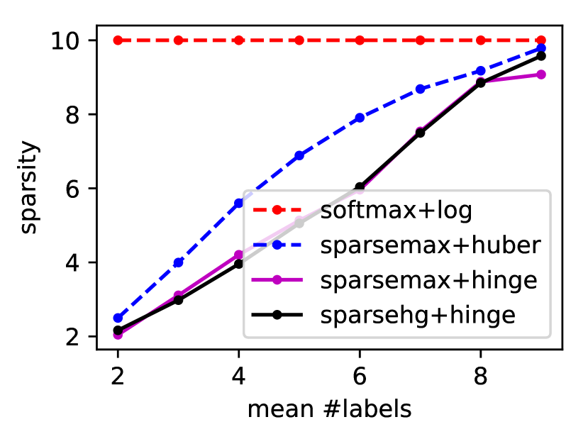
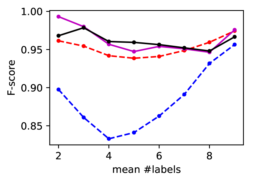
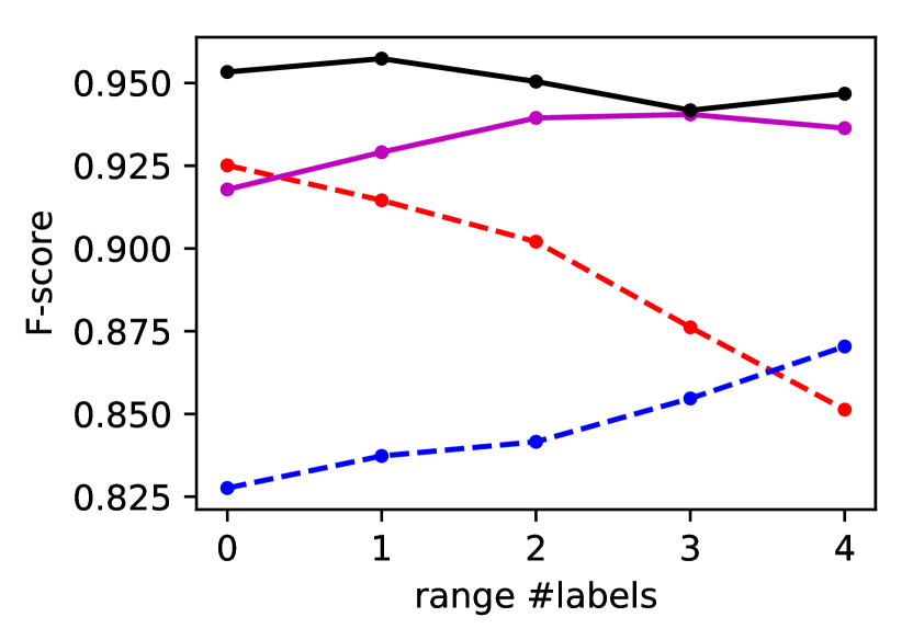
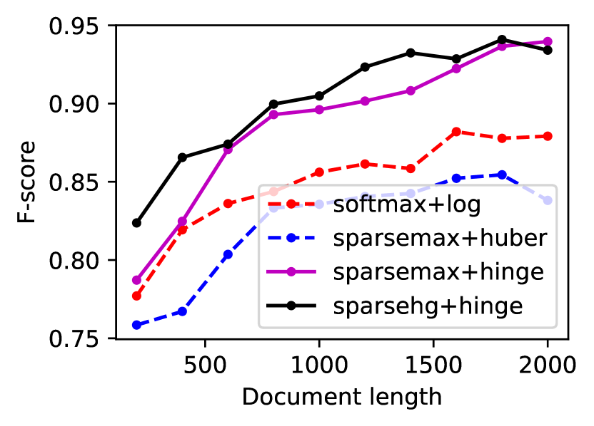
Fig.5 shows F-score on test sets in the three experimental settings. We can observe that sparsemax+hinge and sparsehg+hinge consistently perform better than sparsemax+huber in all three cases, especially the label distributions are sparser. Note that sparsehg+hinge performs better than sparsemax+hinge in most cases. From empirical comparison between sparsemax+hinge and sparsemax+huber, we can conclude that the proposed hinge loss variants are better in producing sparser and and more accurate predictions. This observation is also supported in our analysis of sparsity in outputs (see Fig.4 - lower the curve the sparser it is - this is analysis is done corresponding to the setting in Fig.5(a)), where we find that hinge loss variants encourage more sparsity. We also find the hinge loss variants are doing better than softmax+log in terms of the JSD metric (details in App.A.7.1).

5.1.2 Real Multilabel datasets

We further experiment with three real datasets for multilabel classification: Birds, Scene and Emotions. The experimental setup and baselines are same as that for synthetic dataset described in Sec.5.1.1. For each of the datasets, we consider only those examples with atleast one label. Results are shown in Table 3 in App.A.7.2. All methods give comparable results on these benchmark datasets.

(a) Varying mean #labels

(b) Varying range #labels

(c) Varying document length

Figure 5: F-score on multilabel classification synthetic dataset.

5.2 Sparse Attention for Natural Language Generation

Here we demonstrate the effectiveness of our formulations experimentally on two natural language generation tasks: neural machine translation and abstractive sentence summarization. The purpose of these experiments are two fold: firstly, effectiveness of our proposed formulations sparsegen-lin and sparsehourglass in attention framework on these tasks, and secondly, control over sparsity leads to enhanced interpretability. We borrow the encoder-decoder architecture with attention (see Fig.7 in App.A.8). We replace the softmax function in attention by our proposed functions as well as sparsemax as baseline. In addition we use another baseline where we tune for the temperature in softmax function. More details are provided in App.A.8.

Experimental Setup: In our experiments we adopt the same experimental setup followed by [16] on top of the OpenNMT framework [18]. We varied only the control parameters required by our formulations. The models for the different control parameters were trained for 13 epochs and the epoch with the best validation accuracy is chosen as the best model for that setting. The best control parameter for a formulation is again selected based on validation accuracy. For all our formulations, we report the test scores corresponding to the best control parameter in Table 2.

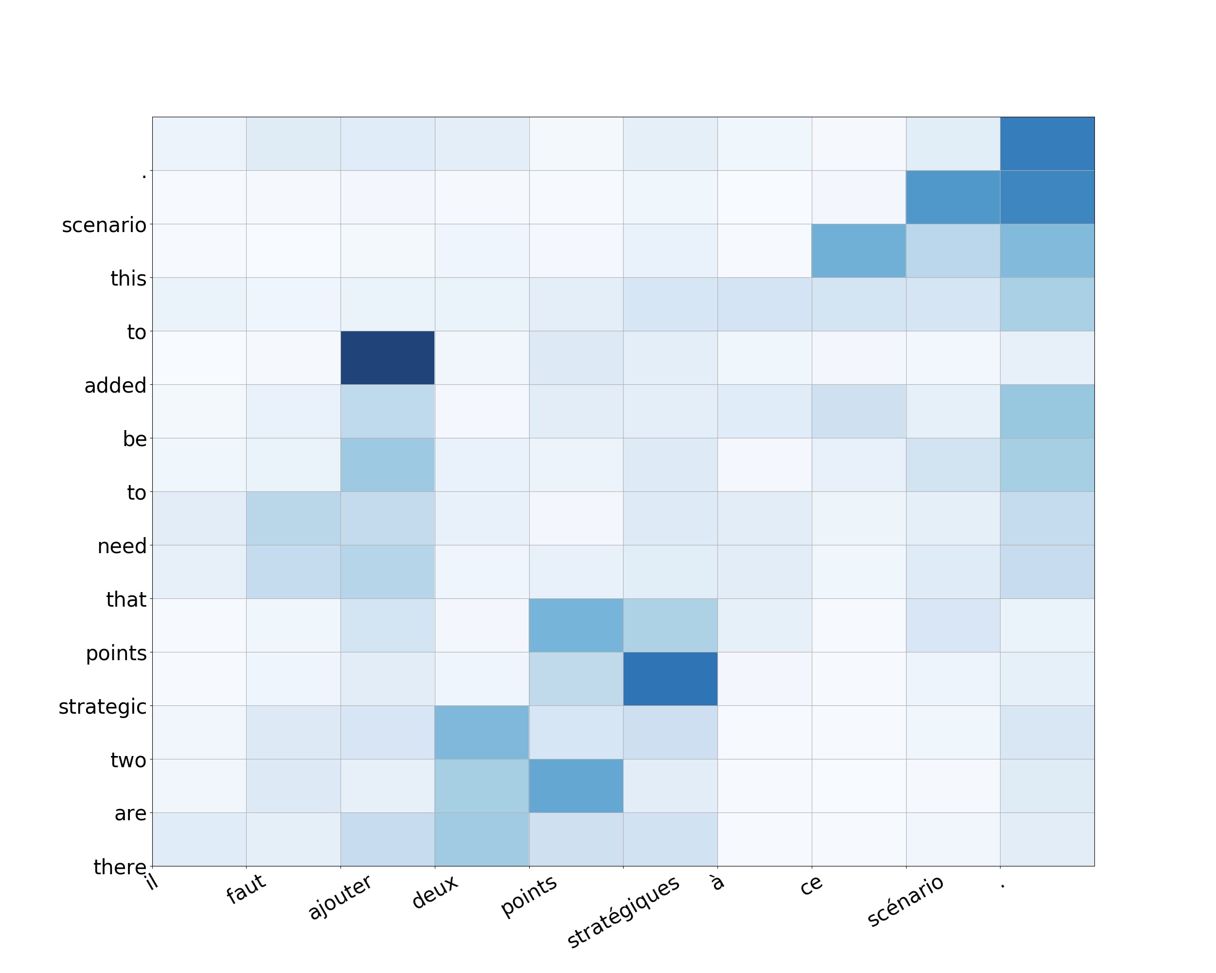
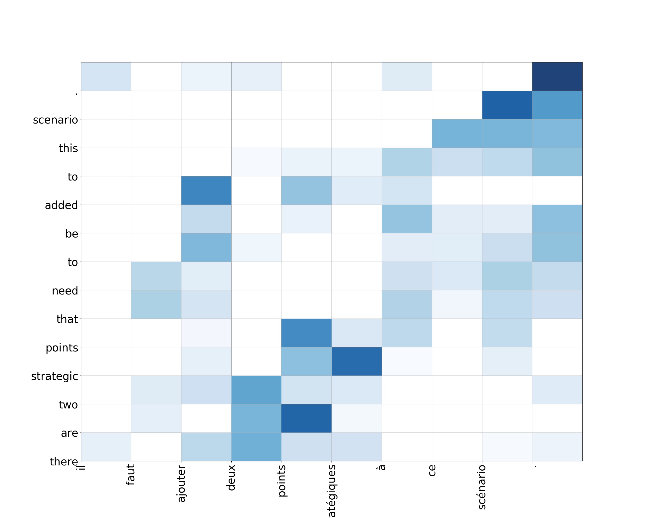
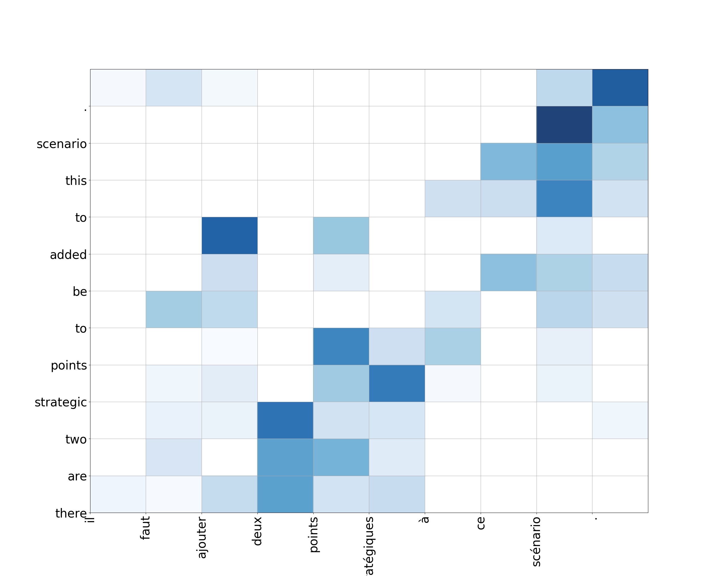
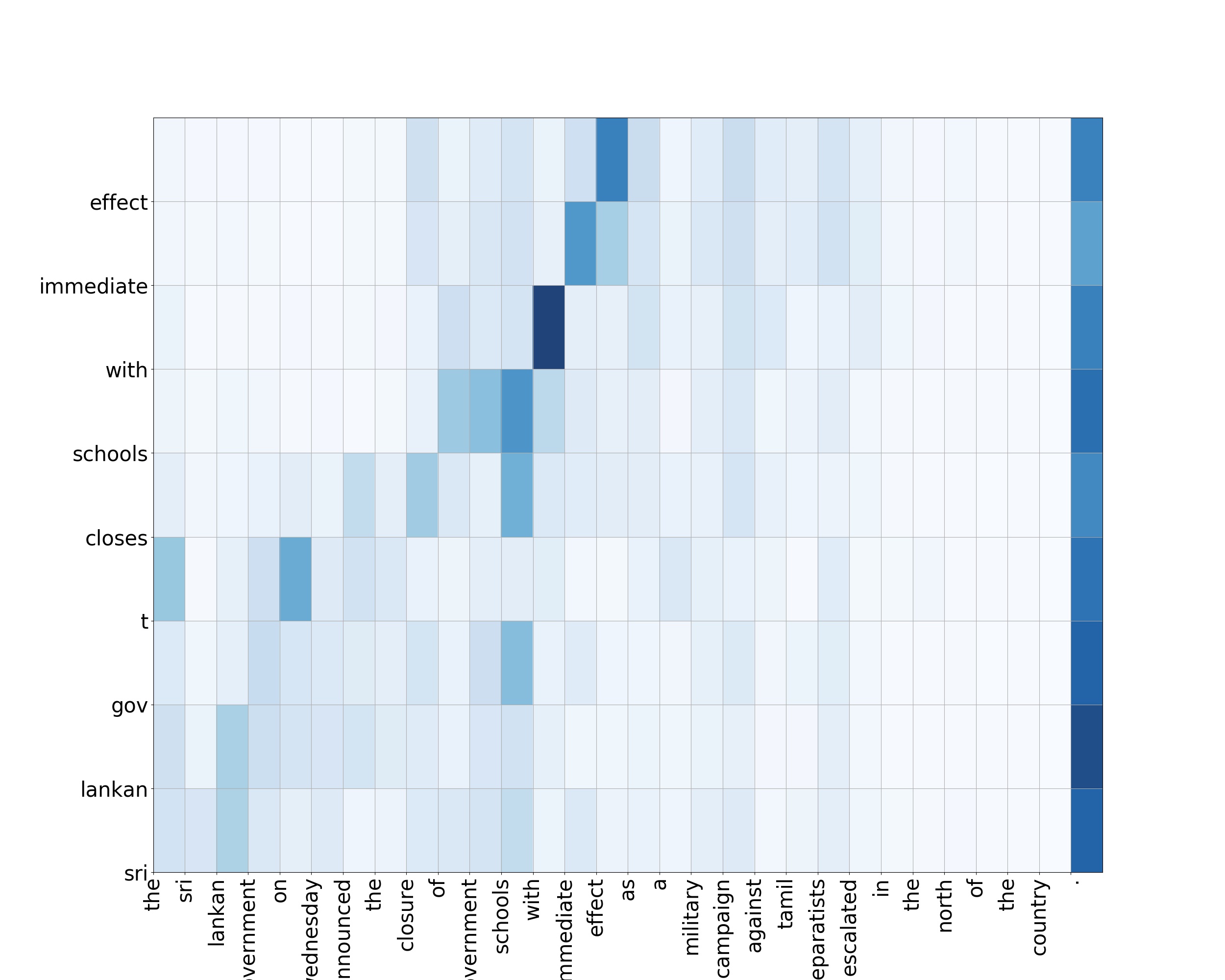
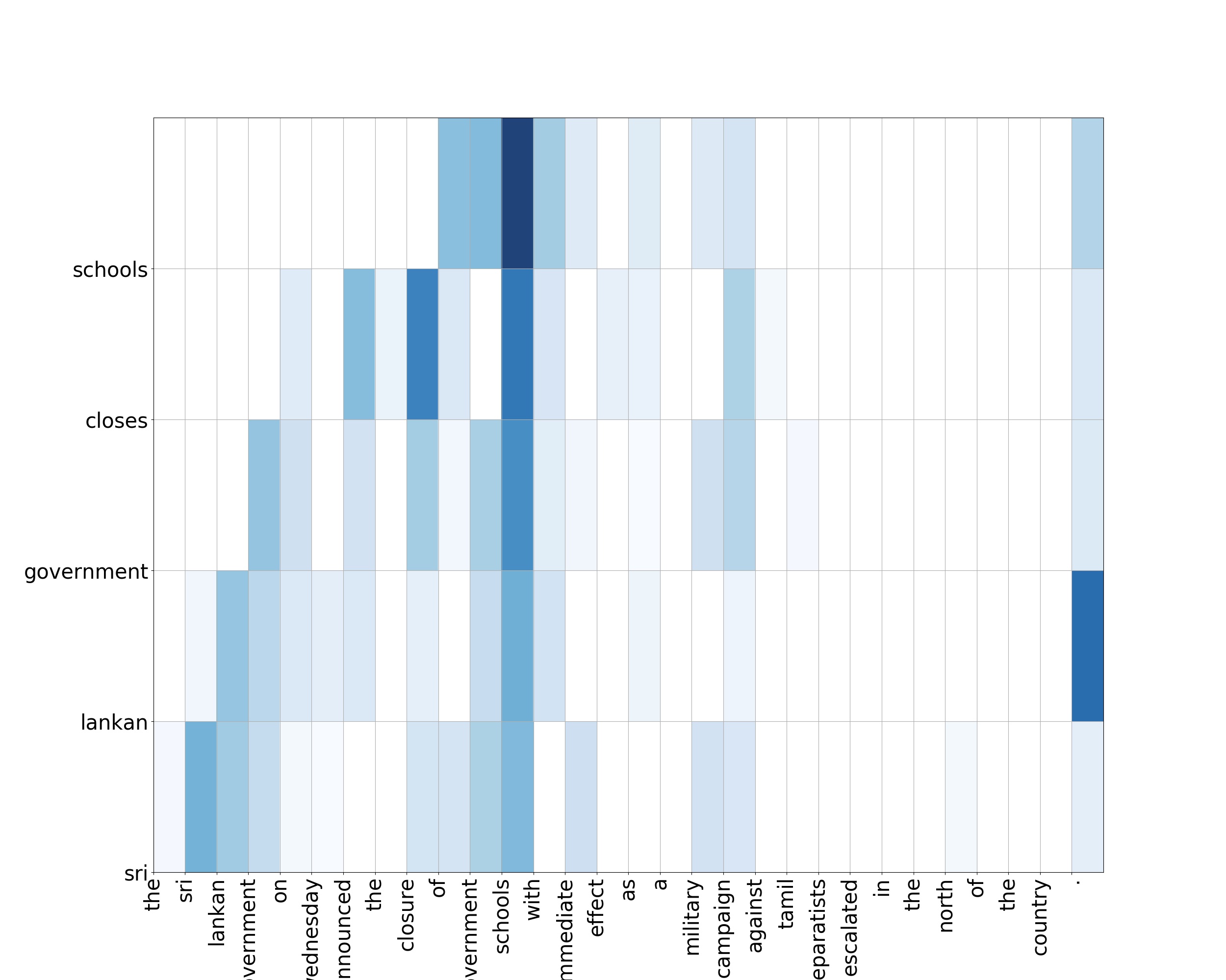
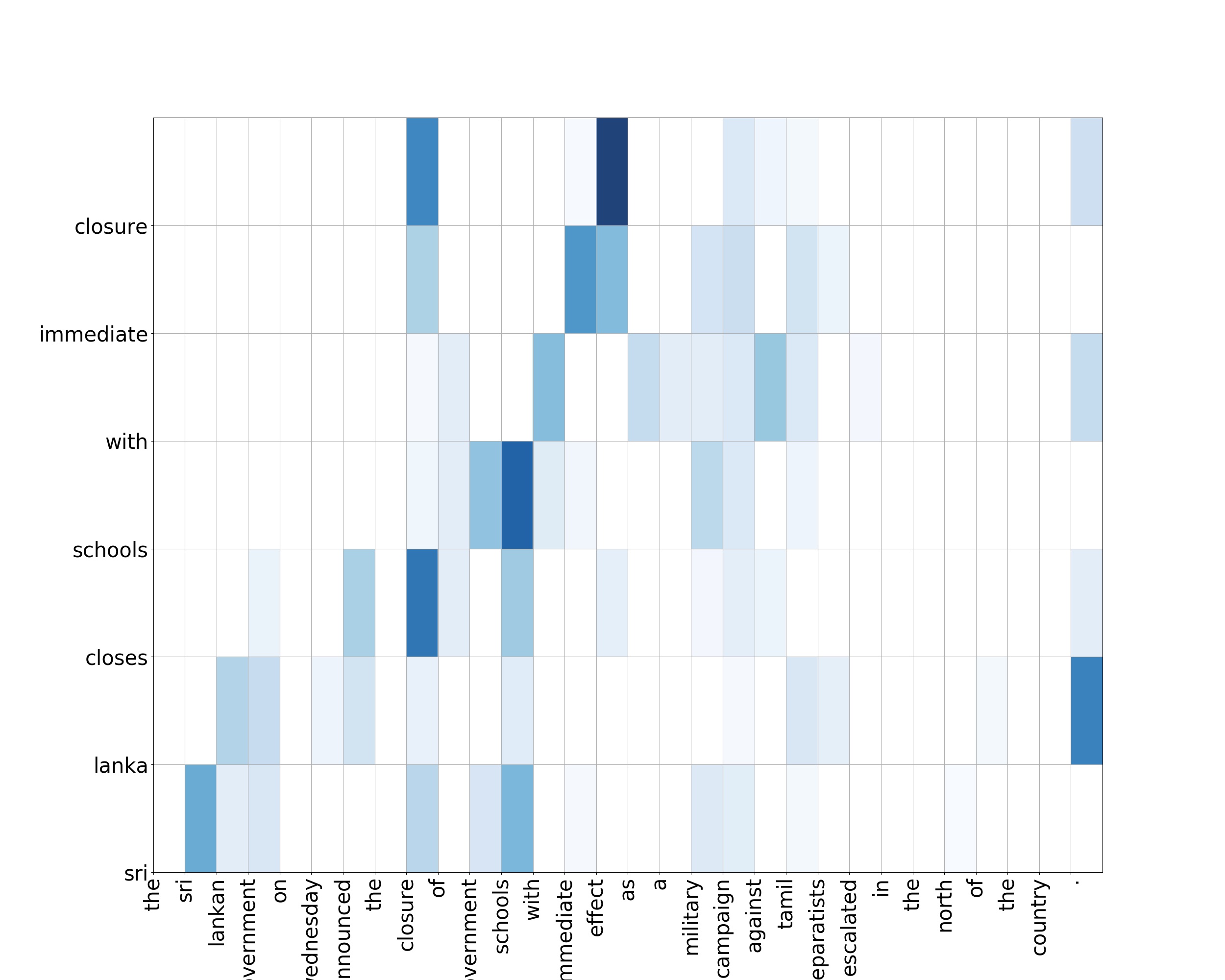
Neural Machine Translation: We consider the FR-EN language pair from the NMT-Benchmark project and perform experiments both ways. We see (refer Table.2) that sparsegen-lin surpasses BLEU scores of softmax and sparsemax for FR-EN translation, whereas sparsehg formulations yield comparable performance. Quantitatively, these metrics show that adding explicit controls do not come at the cost of accuracy. In addition, it is encouraging to see (refer Fig.8 in App.A.8) that increasing $\lambda$ for sparsegen-lin leads to crisper and hence more interpretable attention heatmaps (the lesser number of activated columns per row the better it is). We have also analyzed the average sparsity of heatmaps over the whole test dataset and have indeed observed that larger $\lambda$ leads to sparser attention. Abstractive Summarization: We next perform our experiments on abstractive summarization datasets like Gigaword, DUC2003 & DUC2004 and report ROUGE metrics. The results in Table.2 show that sparsegen-lin stands out in performance with other formulations closely following and comparable to softmax and sparsemax. It is also encouraging to see that all the models trained on Gigaword generalizes well on other datasets DUC2003 and DUC2004. Here again the $\lambda$ control leads to more interpretable attention heatmaps as shown in Fig.9 in App.A.8 and we have also observed the same with average sparsity of heatmaps over the test set.

Attention	Translation		Summarization
	FR-EN	EN-FR	Gigaword			DUC 2003			DUC 2004
	BLEU	BLEU	R-1	R-2	R-L	R-1	R-2	R-L	R-1	R-2	R-L
softmax	36.38	36.00	34.80	16.64	32.15	27.95	9.22	24.54	30.68	12.24	28.12
softmax (with temp.)	36.63	36.08	35.00	17.15	32.57	27.78	8.91	24.53	31.64	12.89	28.51
sparsemax	36.73	35.78	34.89	16.88	32.20	27.29	8.48	24.04	30.80	12.01	28.04
sparsegen-lin	37.27	35.78	35.90	17.57	33.37	28.13	9.00	24.89	31.85	12.28	29.13
sparsehg	36.63	35.69	35.14	16.91	32.66	27.39	9.11	24.53	30.64	12.05	28.18

Table 2: Sparse Attention Results. Here R-1, R-2 and R-L denote the ROUGE scores.

6 Conclusions and Future Work

In this paper, we investigated a family of sparse probability mapping functions, unifying them under a general framework. This framework helped us to understand connections to existing formulations in the literature like softmax, spherical softmax and sparsemax. Our proposed probability mapping functions enabled us to provide explicit control over sparsity to achieve higher interpretability. These functions have closed-form solutions and sub-gradients can be computed easily. We have also proposed convex loss functions, which helped us to achieve better accuracies in the multilabel classification setting. Application of these formulations to compute sparse attention weights for NLP tasks also yielded improvements in addition to providing control to produce enhanced interpretability. As future work, we intend to apply these sparse attention formulations for efficient read and write operations of memory networks [19]. In addition, we would like to investigate application of these proposed sparse formulations in knowledge distillation and reinforcement learning settings.

Acknowledgements

We thank our colleagues in IBM, Abhijit Mishra, Disha Shrivastava, and Parag Jain for the numerous discussions and suggestions which helped in shaping this paper.

Appendix A Supplementary Material

A.1 Closed-Form Solution of Sparsegen

Formulation is given by:

$$\bm{p}^{*}=\text{sparsegen}(\bm{z})=\operatorname*{argmin}_{\bm{p}\in\Delta^{K-1}}\{\|\bm{p}-g(\bm{z})\|^{2}_{2}-\lambda\|\bm{p}\|^{2}_{2}\}$$ (8)

The Lagrangian of the above formulation is:

$$\mathscr{L}(\bm{z},\bm{\mu},\tau)=\frac{1}{2}\|\bm{p}-g(\bm{z})\|^{2}_{2}-\frac{\lambda}{2}\|\bm{p}\|^{2}_{2}-\bm{\mu}^{T}\bm{p}+\tau(\textbf{1}^{T}\bm{p}-1)$$ (9)

Defining the Karush-Kuhn-Tucker conditions with respect to optimal solutions ($\bm{p}^{*},\bm{\mu}^{*},\tau^{*}$):

$$p_{i}^{*}-g_{i}(\bm{z})-\lambda p_{i}^{*}-\mu_{i}^{*}+\tau^{*}=0,\forall i\in[K],$$ (10)

$$\textbf{1}^{T}\bm{p}^{*}=1,\bm{p}^{*}\geq\textbf{0},\bm{\mu}^{*}\geq\textbf{0},$$ (11)

$$\mu_{i}^{*}p_{i}^{*}=0,\forall i\in[K].(\text{complementary slackness})$$ (12)

From Eq.12, if we want $p_{i}^{*}>0$ for certain $i\in[K]$, then we must have $\mu_{i}^{*}=0$. This implies $p_{i}^{*}-g_{i}(\bm{z})-\lambda p_{i}^{*}+\tau^{*}=0$ (according to Eq. 10). This leads to $p_{i}^{*}=(g_{i}(\bm{z})-\tau^{*})/(1-\lambda)$. For $i\notin S(\bm{z})$, where $p_{i}=0$, we have $g_{i}(\bm{z})-\tau^{*}\leq 0$ (as $\mu_{i}^{*}\geq 0$). From Eq. 11 we obtain $\sum_{j\in S(\bm{z})}(g_{j}(\bm{z})-\tau^{*})=1-\lambda$, which leads to $\tau^{*}=(\sum_{j\in S(\bm{z})}g_{j}(\bm{z})-1+\lambda)/|S(\bm{z})|$.

Proposition 0.1

The closed-form solution of sparsegen is as follows ($\forall i\in[K]$):

$$\rho_{i}(\bm{z})=\text{sparsegen}_{i}(\bm{z};g,\lambda)=\Big{[}\frac{g_{i}(\bm{z})-\tau(\bm{z})}{1-\lambda}\Big{]}_{+},$$ (13)

where $\tau(\bm{z})$ is the threshold which makes $\sum_{j\in[K]}\rho_{j}(\bm{z})=1$. Let $g_{(1)}(\bm{z})\geq g_{(2)}(\bm{z})\dots\geq g_{(K)}(\bm{z})$ be the sorted coordinates of $g(\bm{z})$. The cardinality of the support set $S(\bm{z})$ is given by $k(\bm{z}):=\max\{k\in[K]\ |\ 1-\lambda+kg_{(k)}(\bm{z})>\sum_{j\leq k}g_{(j)}(\bm{z})\}$. Then $\tau(\bm{z})$ can be obtained as,

$$\tau(\bm{z})=\frac{\sum_{j\leq k(\bm{z})}g_{(j)}(\bm{z})-1+\lambda}{k(\bm{z})}=\frac{\sum_{j\in S(\bm{z})}g_{j}(\bm{z})-1+\lambda}{|S(\bm{z})|},$$

A.2 Special cases of Sparsegen

Example 1: $\bm{g(\bm{z})=\bm{z}}$ (sparsegen-lin):
When $g(\bm{z})=\bm{z}$, sparsegen reduces to a regularized extension of sparsemax. This is translation invariant, has monotonicity and can work for full domain. It is also Lipschitz continuous with the Lipschitz constant being $1/(1-\lambda)$. The visualization of this variant is shown in Fig.2.

Example 2: $\bm{g(z)=\text{exp}(z)}$ (sparsegen-exp):
$\text{exp}(\bm{z})$ here means element-wise exponentiation of $\bm{z}$, that is $g_{i}(\bm{z})=\text{exp}(z_{i})$. For $\bm{z}$ where all $z_{i}>0$, sparsegen-exp leads to sparser solutions than sparsemax.

Checking with properties from Sec.3.3, sparsegen-exp satisfies monotonicity as $\text{exp}(z_{i})$ is a monotonically increasing function. However, as $\text{exp}(\bm{z})$ is not Lipschitz continuous, sparsegen-exp is not Lipschitz continuous.

It is interesting to note that sparsegen-exp reduces to softmax when $\lambda$ is dependent on $\bm{z}$ and equals $1-\sum_{j\in[K]}e^{z_{j}}$, as it results in $\tau(\bm{z})=0$ and $S(\bm{z})=[K]$ according to Eq.13.

Example 3: $\bm{g(z)=z^{2}}$ (sparsegen-sq):

Unlike sparsegen-lin and sparsegen-exp, sparsegen-sq does not satisfy the monotonicity property as $g_{i}(\bm{z})=z_{i}^{2}$ is not monotonic. Also sparsegen-sq has neither translation invariance nor scale invariance. Moreover, as $\bm{z}^{2}$ is not Lipschitz continuous, sparsegen-sq is not Lipschitz continuous. Additionally, when $\lambda$ depends on $\bm{z}$ and $\lambda=1-\sum_{j\in[K]}z^{2}_{j}$, sparsegen-sq reduces to spherical softmax.

Example 4: $\bm{g(z)=log(z)}$ (sparsegen-log):
$\text{log}(\bm{z})$ here means element-wise natural logarithm of $\bm{z}$, that is $g_{i}(\bm{z})=\text{log}(z_{i})$. This is scale invariant but not translation invariant. However, it is not defined for negative values or zero values of $z_{i}$.

A.3 Derivation of Sparsecone

Let us project a point $\bm{z}=(z_{1},\dots,z_{K})\in\mathbb{R}^{K}$ onto the simplex along the line connecting $\bm{z}$ with $\bm{q}=(-q,\dots,-q)\in\mathbb{R}^{K}$. The equation of this line is $\alpha\bm{z}+(1-\alpha)\bm{q}$. If the point of intersection of the line with the probability simplex (denoted by $\bm{1}^{T}\bm{z}=1$) is represented as $\bm{\hat{z}}=\alpha^{*}\bm{z}+(1-\alpha^{*})\bm{q}$, then it should have the property: $\sum_{i}\hat{z}_{i}=\alpha^{*}\sum_{i}z_{i}-(1-\alpha^{*})Kq=1$, which leads to $\alpha^{*}=(1+Kq)/(\sum_{i}z_{i}+Kq)$. Also, $\hat{z}_{i}\geq 0$ condition must be satisfied, as it should lie on the probability simplex. Thus, the required point can be obtained by solving the following:

$$\bm{p}^{*}=\operatorname*{argmin}_{\bm{p}\in\Delta^{K-1}}\|\bm{p}-\bm{\hat{z}}\|^{2}_{2} =\operatorname*{argmin}_{\bm{p}\in\Delta^{K-1}}\|\bm{p}-\alpha^{*}\bm{z}-(1-\alpha^{*})\bm{q}\|^{2}_{2},$$ (14)

$$=\operatorname*{argmin}_{\bm{p}\in\Delta^{K-1}}\|\bm{p}-\alpha^{*}\bm{z}\|^{2}_{2}=\text{sparsemax}(\alpha^{*}\bm{z}),$$ (15)

$$\alpha^{*} =\frac{1+Kq}{\sum_{i\in[K]}z_{i}+Kq}$$ (16)

As $\alpha^{*}$ is a function of $\bm{z}$, it is denoted by $\alpha(\bm{z})$. The formulation in Eq.14 is equivalent to Eq.15, utilizing the translation invariance property of sparsemax as $(1-\alpha^{*})\bm{q}$ is a constant term for a particular $\bm{z}$. Thus, we can say sparsecone can be obtained by $\text{sparsemax}(\alpha(\bm{z})\bm{z})$, where $\alpha(\bm{z})$ is given by Eq.16.

A.4 Derivation of Sparsehourglass

The above formulation fails for $\bm{z}$ such that $\sum_{i}z_{i}<-Kq$. For example, it fails for $\bm{z}=(-2,-1)$, where $\bm{q}=(-1,-1)$ (the solution will give greater probability mass to -2 compared to -1), that is $q=1$. To make it work for such a $\bm{z}$, we can find a mirror point $\tilde{\bm{z}}$ satisfying the following properties : (1) $\sum_{i}\tilde{z}_{i}=-\sum_{i}z_{i}$, and (2) $\tilde{z}_{i}-\tilde{z}_{j}=z_{i}-z_{j}\forall(i,j)$, and (3) $\text{sparsehourglass}(\bm{z})=\text{sparsecone}(\tilde{\bm{z}})$. Let $\text{sparsecone}(\tilde{\bm{z}})$ be given by $\text{sparsemax}(\alpha(\tilde{\bm{z}})\tilde{\bm{z}})$ (as seen earlier) and $\text{sparsehourglass}(\bm{z})$ be defined by $\text{sparsemax}(\alpha^{*}\bm{z})$. Can we find $\alpha^{*}$ which satisfies the mirror point properties above? Property (3) is true iff $\alpha(\tilde{\bm{z}})(\tilde{z_{i}}-\tilde{z_{j}})=\alpha^{*}(z_{i}-z_{j})\forall(i,j)$. Using property (2) we get, $\alpha(\tilde{\bm{z}})=\alpha^{*}$. From definition of sparsecone, $\alpha(\tilde{\bm{z}})=(1+Kq)/(\sum_{i}\tilde{z_{i}}+Kq)$. Using property (1), we get $\alpha^{*}=\alpha(\tilde{\bm{z}})=(1+Kq)/(\sum_{i}\tilde{z_{i}}+Kq)=(1+Kq)/(-\sum_{i}z_{i}+Kq)$. As $\alpha^{*}$ is a function of $\bm{z}$, let it be represented as $\hat{\alpha}(\bm{z})$. Thus, sparsehourglass is defined as follows:

$$\bm{p}^{*}=\text{sparsehourglass}(\bm{z}) =\operatorname*{argmin}_{\bm{p}\in\Delta^{K-1}}\|\bm{p}-\hat{\alpha}(\bm{z})\bm{z}\|^{2}_{2}$$ (17)

$$=\text{sparsemax}(\hat{\alpha}(\bm{z})\bm{z})$$ (18)

$$\hat{\alpha}(\bm{z}) =\frac{1+Kq}{|\sum_{i\in[K]}z_{i}|+Kq}$$ (19)

A.5 Proof for Lipschitz constant of Sparsehourglass

Lipschitz constant of composition of functions is bounded above by the product of Lipschitz constants of functions in the composition. Applying this principle on Eq.18 we find an upper bound for the Lipschitz constant of sparsehg (denoted as $L_{\text{sparsehg}}$) as the product of Lipschitz constant of sparsemax (denoted as $L_{\text{sparsemax}}$) and Lipschitz constant of $g(\bm{z})=\hat{\alpha}(\bm{z})\bm{z}$ (which we denote as $L_{g}$).

$$L_{\text{sparsehg}}\leq L_{\text{sparsemax}}\times L_{g}$$ (20)

We use the property that Lipschitz constant of a function is the largest matrix norm of Jacobian of that function. For sparsemax that would be,

$$L_{\text{sparsemax}} =\operatorname*{argmax}_{\bm{x},\bm{z}\in\mathbb{R}^{K}}\,\frac{\|J_{\text{sparsemax}}(\bm{z})\bm{x}\|_{2}}{\|\bm{x}\|_{2}}$$

where, $J_{\text{sparsemax}}(\bm{z})$ is the Jacobian of sparsemax at given value $\bm{z}$. From the term given in Sec.3, $J_{\text{sparsemax}}(\bm{z})=\Big{[}\text{Diag}(\bm{s})-\frac{\bm{s}\bm{s}^{T}}{|S(\bm{z})|}\Big{]}$ whose matrix norm is $1$. We use the property that, for any symmetric matrix, matrix norm is the largest absolute eigenvalue, and the eigenvalues of $J_{\text{sparsemax}}(\bm{z})$ are $0$ and $1$. Hence, $L_{\text{sparsemax}}=1$.

For $g(\bm{z})=\hat{\alpha}(\bm{z})\bm{z}$, let us look at the Jacobian of $g(\bm{z})$, which is given as

$$J_{g}(\bm{z})=\hat{\alpha}(\bm{z})\mathbf{I}\,-\,\frac{\hat{\alpha}(\bm{z})\,\text{sgn}(\sum_{i}z_{i})}{|\sum_{i}z_{i}|+Kq}\,\begin{bmatrix}z_{1}&z_{1}&\dots&z_{1}\\ z_{2}&z_{2}&\dots&z_{2}\\ \vdots&\ddots&&\\ z_{K}&&&z_{K}\end{bmatrix},$$ (21)

where $\mathbf{I}$ denotes identity matrix. Eigen values of $J_{g}(\bm{z})$ are $\hat{\alpha}(\bm{z})$ and $\hat{\alpha}(\bm{z})(1-\frac{|\sum z_{i}|}{|\sum z_{i}|+Kq})$, and the largest among them is clearly $\hat{\alpha}(\bm{z})$. As $\hat{\alpha}(\bm{z})>0$, all the eigen values of $J_{g}(\bm{z})$ are greater than 0, making $J_{g}(\bm{z})$ a positive definite matrix. We now use the property that for any positive definite matrix, matrix norm is the largest eigenvalue. From Eq.19, we see that the largest eigen value of $J_{g}(\bm{z})$ is $\hat{\alpha}(\bm{z})$ which assumes the largest value when $\sum_{i}z_{i}=0$. The highest value of $\hat{\alpha}(\bm{z})$ is $1+\frac{1}{Kq}$; therefore, $L_{g}=1+\frac{1}{Kq}$. Thus,

$$L_{\text{sparsehg}}\leq L_{\text{sparsemax}}\times L_{g}=1\times(1+\frac{1}{Kq})=1+\frac{1}{Kq}$$

It turns out this is also a tight bound; hence, $L_{\text{sparsehg}}=1+\frac{1}{Kq}$.

A.6 Synthetic dataset creation

We use scikit-learn for generating synthetic datasets with 5000 instances split across train (0.5), val (0.2) and test (0.3). Each instance is a multilabel document with a sequence of words. Vocabulary size and number of labels $K$ are fixed to $10$. Each instance is generated as follows: We draw number of true labels $N\in\{1,\dots,K\}$ from either a discrete uniform distribution. Then we sample $N$ labels from $\{1,\dots,K\}$ without replacement and sample $L$ number of words (document length) from the mixture of sampled label-specific distribution over words.

A.7 More results on multilabel classification experiments

A.7.1 Synthetic Dataset

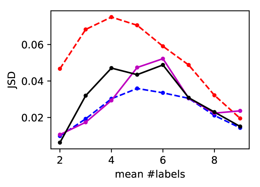
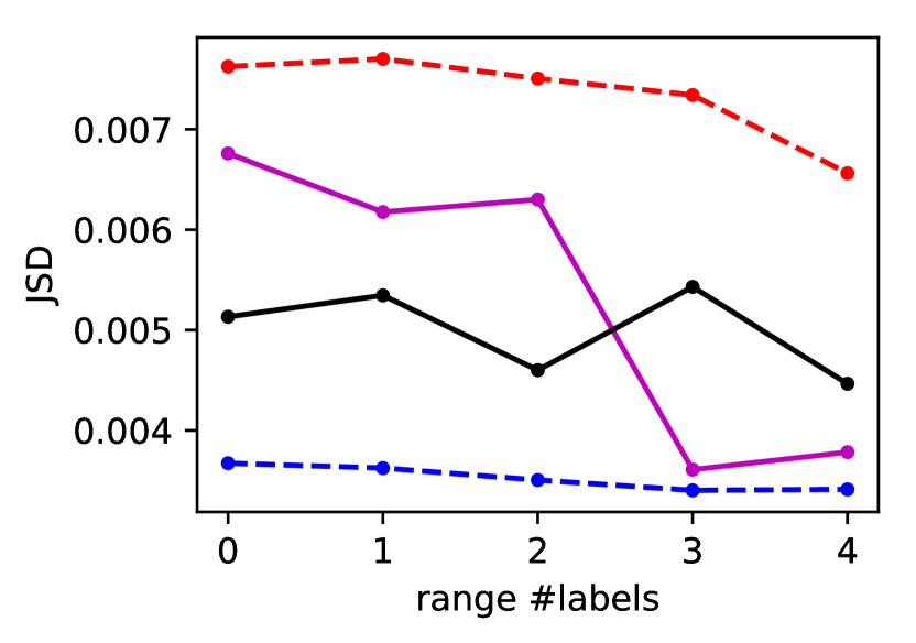
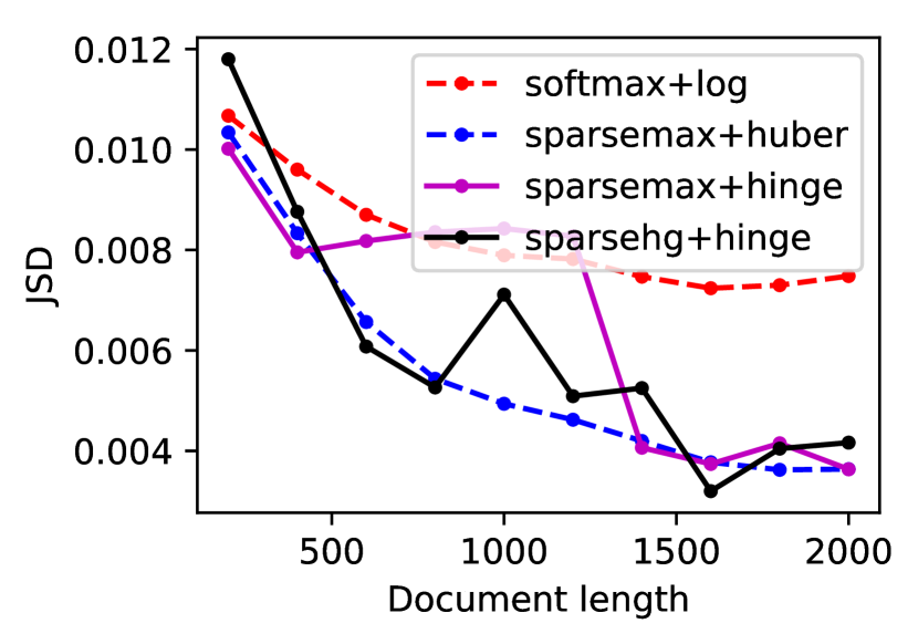
Fig.6 shows JSD between normalized true label and predicted distribution. Though sparsemax+huber is performing overall the best, in the case when number of labels is small we could see sparsehg+hinge and sparsemax+hinge performing as good as sparsemax+huber. In general we could see that sparsehg+hinge is performing better than sparsemax+hinge, which in turn is better than softmax+log.

(a) Varying mean #labels

(b) Varying range #labels

(c) Varying document length

Figure 6: JSD on multilabel classification synthetic dataset

A.7.2 Real Datasets

Activation + Loss	SCENE	EMOTIONS	BIRDS
softmax+log	0.71	0.65	0.43
sparsemax+huber	0.70	0.63	0.42
sparsemax+hinge	0.68	0.65	0.41
sparsehg+hinge	0.69	0.65	0.41

Table 3: F-score on three benchmark multilabel datasets

A.8 Controlled Sparse Attention

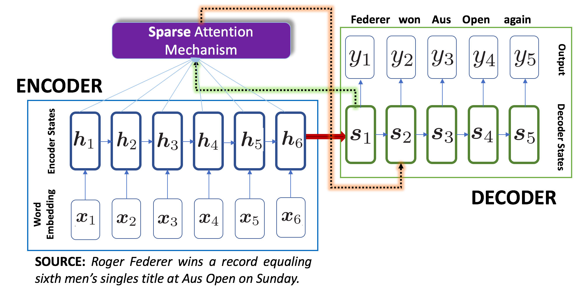
Here we discuss attention mechanism with respect to encoder-decoder architecture as illustrated in Fig. 7. Lets say we have a sequence of inputs (possibly sequence of words) and their corresponding word vectors sequence be $\bm{X}=(\bm{x}_{1},\dots,\bm{x}_{K})$. The task will be to produce a sequence of words $\bm{Y}=(y_{1},\dots,y_{L})$ as output. Here an encoder RNN encodes the input sequence into a sequence of hidden state vectors $\bm{H}=(\bm{h}_{1},\dots,\bm{h}_{K})$. A decoder RNN generates its sequence of hidden states $\bm{S}=(\bm{s}_{1},\dots,\bm{s}_{L})$ by considering different $\bm{h}_{i}$ while generating different $\bm{s}_{j}$. This is known as hard attention. This approach is known to be non-differentiable as it is based on a sampling based approach [6]. As an alternative solution, a softer version (called soft attention) is more popularly used. It involves generating a score vector $\bm{z}_{t}=(z_{t1},\dots,z_{tK})$ based on relevance of encoder hidden states $\bm{H}$ with respect to current decoder state vector $\bm{s}_{t}$ using Eq.22. The score vector is then transformed to a probability distribution using the Eq.23. Considering the attention model parameters [$\bm{W}_{s}$, $\bm{W}_{h}$, $\bm{v}$], we define the following:

$$z_{ti}=\bm{v}^{T}\text{tanh}(\bm{W}_{s}\bm{s}_{t}+\bm{W}_{h}\bm{h}_{i}).$$ (22)

$$\bm{p}_{t}=softmax(\bm{z}_{t})$$ (23)

Following the approach by [14], we replace Eq.23 with our formulations, namely, sparsegen-lin and sparsehourglass. This enables us to apply explicit control over the attention weights (with respect to sparsity and tradeoff between scale and translation invariance) produced for the sequence to sequence architecture. This falls in the sparse attention paradigm as proposed in the earlier work. Unlike hard attention, these formulations lead to easy computation of sub-gradients, thus enabling backpropagation in this encoder-decoder architecture composed RNNs. This approach can also be extended to other forms of non-sequential input (like images) as long as we can compute the score vector $\bm{z}_{t}$ from them, possibly using a different encoder like CNN instead of RNN.

Figure 7: Encoder Decoder with Sparse Attention

A.8.1 Neural Machine Translation

The first task we consider for our experiments is neural machine translation. Our aim is to see how our techniques compare with softmax and sparsemax with respect BLEU metric and interpretability. We consider the french-english language pair from the NMT-Benchmark project and perform experiments both ways using controlled sparse attention. The dataset has around 1M parallel training instances along with equal validation and test sets of 1K parallel instances.

We find from our experiments (refer Table.2) that sparsegen-lin surpasses the BLEU scores of softmax and sparsemax for FR-EN translation, whereas the other formulations yield comparable performance. On the other hand, for EN-FR translation, softmax is still better than others. Quantitatively, these metrics show that adding explicit controls do not come at the cost of accuracy. In addition, it is encouraging to see (refer Fig.8) that increasing $\lambda$ for sparsegen-lin leads to crisper and hence more interpretable attention heatmaps (the lesser number of activated columns per row the better it is).

A.8.2 Abstractive Summarization

We next perform our experiments on abstractive summarization datasets like Gigaword, DUC2003 & DUC2004. This dataset consists of pairs of sentences where the task is to generate the second sentence (news headline) as a summary of the larger first sentence. We trained our models on nearly 4M training pairs of Gigaword and validated on 190K pairs. Then we reported the test scores according to ROUGE metrics on 2K test instances of Gigaword, 624 instances of DUC2003 and 500 instances of DUC2004.

The results in Table.2 show that sparsegen-lin stands out in performance amongst other formulations with the other formulations closely following and comparable to softmax and sparsemax. It is also encouraging to see that all the models trained on Gigaword generalizes well on other datasets DUC2003 and DUC2004. Here again the $\lambda$ control leads to more interpretable attention heatmaps as shown in Fig.9.

Figure 8: The attention heatmaps for softmax, sparsemax and sparsegen-lin ($\lambda=0.75$) in translation (FR-EN) task.

Figure 9: The attention heatmaps for softmax, sparsemax and sparsegen-lin ($\lambda=0.75$) in summarization (Gigaword) task.

References

- [1] M. Aly. Survey on multiclass classification methods. Neural networks, pages 1–9, 2005.
- [2] John S. Bridle. Probabilistic interpretation of feedforward classification network outputs, with relationships to statistical pattern recognition. In Françoise Fogelman Soulié and Jeanny Hérault, editors, Neurocomputing, pages 227–236, Berlin, Heidelberg, 1990. Springer Berlin Heidelberg.
- [3] Richard S. Sutton and Andrew G. Barto. Introduction to Reinforcement Learning. MIT Press, Cambridge, MA, USA, 1st edition, 1998.
- [4] B. Gao and L. Pavel. On the properties of the softmax function with application in game theory and reinforcement learning. ArXiv e-prints, 2017.
- [5] Dzmitry Bahdanau, Kyunghyun Cho, and Yoshua Bengio. Neural machine translation by jointly learning to align and translate. In Proceedings of the International Conference on Learning Representations (ICLR), San Diego, CA, 2015.
- [6] Kelvin Xu, Jimmy Ba, Ryan Kiros, Kyunghyun Cho, Aaron C. Courville, Ruslan Salakhutdinov, Richard S. Zemel, and Yoshua Bengio. Show, attend and tell: Neural image caption generation with visual attention. In Francis R. Bach and David M. Blei, editors, ICML, volume 37 of JMLR Workshop and Conference Proceedings, pages 2048–2057. JMLR.org, 2015.
- [7] K. Cho, A. Courville, and Y. Bengio. Describing multimedia content using attention-based encoder-decoder networks. IEEE Transactions on Multimedia, 17(11):1875–1886, Nov 2015.
- [8] Alexander M. Rush, Sumit Chopra, and Jason Weston. A neural attention model for abstractive sentence summarization. In Proceedings of the 2015 Conference on Empirical Methods in Natural Language Processing, pages 379–389, Lisbon, Portugal, September 2015. Association for Computational Linguistics.
- [9] Preksha Nema, Mitesh Khapra, Anirban Laha, and Balaraman Ravindran. Diversity driven attention model for query-based abstractive summarization. In Proceedings of the 55th Annual Meeting of the Association for Computational Linguistics, Vancouver, Canada, August 2017. Association for Computational Linguistics.
- [10] Francis Bach, Rodolphe Jenatton, and Julien Mairal. Optimization with Sparsity-Inducing Penalties (Foundations and Trends(R) in Machine Learning). Now Publishers Inc., Hanover, MA, USA, 2011.
- [11] Mohammad S. Sorower. A literature survey on algorithms for multi-label learning. 2010.
- [12] Pascal Vincent, Alexandre de Brébisson, and Xavier Bouthillier. Efficient exact gradient update for training deep networks with very large sparse targets. In Proceedings of the 28th International Conference on Neural Information Processing Systems - Volume 1, NIPS’15, pages 1108–1116, Cambridge, MA, USA, 2015. MIT Press.
- [13] Alexandre de Brébisson and Pascal Vincent. An exploration of softmax alternatives belonging to the spherical loss family. In Proceedings of the International Conference on Learning Representations (ICLR), 2016.
- [14] André F. T. Martins and Ramón F. Astudillo. From softmax to sparsemax: A sparse model of attention and multi-label classification. In Proceedings of the 33rd International Conference on International Conference on Machine Learning - Volume 48, ICML’16, pages 1614–1623. JMLR.org, 2016.
- [15] John Duchi, Shai Shalev-Shwartz, Yoram Singer, and Tushar Chandra. Efficient projections onto the l1-ball for learning in high dimensions. In Proceedings of the 25th International Conference on Machine Learning, ICML ’08, pages 272–279, New York, NY, USA, 2008. ACM.
- [16] Vlad Niculae and Mathieu Blondel. A regularized framework for sparse and structured neural attention. In I. Guyon, U. V. Luxburg, S. Bengio, H. Wallach, R. Fergus, S. Vishwanathan, and R. Garnett, editors, Advances in Neural Information Processing Systems 30, pages 3340–3350. Curran Associates, Inc., 2017.
- [17] Ashish Kapoor, Raajay Viswanathan, and Prateek Jain. Multilabel classification using bayesian compressed sensing. In F. Pereira, C. J. C. Burges, L. Bottou, and K. Q. Weinberger, editors, Advances in Neural Information Processing Systems 25, pages 2645–2653. Curran Associates, Inc., 2012.
- [18] Guillaume Klein, Yoon Kim, Yuntian Deng, Jean Senellart, and Alexander M. Rush. Opennmt: Open-source toolkit for neural machine translation. CoRR, abs/1701.02810, 2017.
- [19] Sainbayar Sukhbaatar, arthur szlam, Jason Weston, and Rob Fergus. End-to-end memory networks. In C. Cortes, N. D. Lawrence, D. D. Lee, M. Sugiyama, and R. Garnett, editors, Advances in Neural Information Processing Systems 28, pages 2440–2448. Curran Associates, Inc., 2015.