Semi-crowdsourced Clustering with
Deep Generative Models

Yucen Luo,  Tian Tian,  Jiaxin Shi,  Jun Zhu,  Bo Zhang
Dept. of Comp. Sci. & Tech., Institute for AI, THBI Lab, BNRist Center,
State Key Lab for Intell. Tech. & Sys., Tsinghua University, Beijing, China
{luoyc15,shijx15}@mails.tsinghua.edu.cn, rossowhite@163.com
{dcszj,dcszb}@mail.tsinghua.edu.cn
corresponding author
Abstract

We consider the semi-supervised clustering problem where crowdsourcing provides noisy information about the pairwise comparisons on a small subset of data, i.e., whether a sample pair is in the same cluster. We propose a new approach that includes a deep generative model (DGM) to characterize low-level features of the data, and a statistical relational model for noisy pairwise annotations on its subset. The two parts share the latent variables. To make the model automatically trade-off between its complexity and fitting data, we also develop its fully Bayesian variant. The challenge of inference is addressed by fast (natural-gradient) stochastic variational inference algorithms, where we effectively combine variational message passing for the relational part and amortized learning of the DGM under a unified framework. Empirical results on synthetic and real-world datasets show that our model outperforms previous crowdsourced clustering methods.

1 Introduction

Clustering is a classic data analysis problem when the taxonomy of data is unknown in advance. Its main goal is to divide samples into disjunct clusters based on the similarity between them. Clustering is useful in various application areas including computer vision [20], bioinformatics [27], anomaly detection [2], etc. When the feature vectors of samples are observed, most clustering algorithms require a similarity or distance metric defined in the feature space, so that the optimization objective can be built. Since different metrics may result in entirely different clustering results, and general geometry metrics may not meet the intention of the tasks’ designer, many clustering approaches learn the metric from the side-information provided by domain experts [29], thus the manual labeling procedure of experts could be a bottleneck for the learning pipeline.

Crowdsourcing is an efficient way to collect human feedbacks [12]. It distributes micro-tasks to a group of ordinal web workers in parallel, so the whole task can be done fast with relatively low cost. It has been used on annotating large-scale machine learning datasets such as ImageNet [6], and can also be used to collect side-information for clustering. However, directly collecting labels from crowds may lead to low-quality results due to the lack of expertise of workers. Consider an example of labeling a set of images of flowers from different species. One could show images to the web workers and ask them to identify the corresponding species, but such tasks require the workers to be experts in identifying the flowers and have all the species in their minds, which is not always possible. A more reasonable and easier task is to ask the workers to compare pairs of flower images and to answer whether they are in the same species or not. Then specific clustering methods are required to discover the clusters from the noisy feedbacks.

To solve above clustering problems with pairwise similarity labels between samples from the crowds, Crowdclustering [8] discovers the clusters within the dataset using a Bayesian hierarchical model. By explicitly modeling the mistakes and preferences of web workers, the outputs will match the human consciousness of the clustering tasks. This method reduces the labeling cost to a great degree compared with expert labeling. However, the cost still grows quadratically as the dataset size grows, so it is still only suitable for small datasets. In this work, we move one step further and consider the semi-supervised crowdclustering problem that jointly models the feature vectors and the crowdsourced pairwise labels for only a subset of samples. When we control the size of the subset to be labeled by crowds, the total labeling budget and time can be controlled. A similar problem has been discussed by [30], while the authors use a linear similarity function defined on the low-level object features, and ignore the noise and inter-worker variations in the manual annotations.

Different from existing approaches, we propose a semi-supervised deep Bayesian model to jointly model the generation of the labels and the raw features for both crowd-labeled and unlabeled samples. Instead of the direct usage of low-level features, we build a flexible deep generative model (DGM) to capture the latent representation of data, which is more suitable to express the semantic similarity than the low-level features. The crowdsourced pairwise labels are modeled by a statistical relational model, and the two parts (i.e., DGM and the relational model) share the same latent variables. We also investigate the fully Bayesian variant of this model so that it can automatically control its complexity. Due to the intractability of exact inference, we develop fast (natural-gradient) stochastic variational inference algorithms. To address the challenges in fully Bayesian inference over model parameters, we effectively combine variational message passing and natural gradient updates for the conjugate part (i.e., the relational model and the mixture model) and amortized learning of the nonconjugate part (i.e., DGM) under a unified framework. Empirical results on synthetic and real-world datasets show that our model outperforms previous crowdsourced clustering methods.

2 Semi-crowdsourced deep clustering

𝐨𝐨\mathbf{o}𝐱𝐱\mathbf{x}𝐳𝐳\mathbf{z}𝜸𝜸{\bm{\gamma}}𝐋𝐋\mathbf{L}α𝛼\alphaβ𝛽\beta𝝅𝝅{\bm{\pi}}𝝁𝝁{\bm{\mu}}, 𝚺𝚺{\bm{\Sigma}}N𝑁NM𝑀M
Figure 1: Semi-crowdsourced Deep Clustering (SCDC).

In this section, we propose the semi-crowdsourced clustering with deep generative models for directly modeling the raw data, which enables end-to-end training. We call the model Semi-crowdsourced Deep Clustering (SCDC), whose graphical model is shown in Figure 1. This model is composed of two parts: the raw data model handles the generative process of the observations 𝐎𝐎\mathbf{O}; the crowdsourcing behavior model on labels 𝐋𝐋\mathbf{L} describes the labeling procedure of the workers. The details for each part will be introduced below.

2.1 Model the raw data – deep generative models

We denote the raw data observations by 𝐎={𝐨1,,𝐨N}𝐎subscript𝐨1subscript𝐨𝑁\mathbf{O}=\{\mathbf{o}_{1},...,\mathbf{o}_{N}\}. For images, 𝐨nDsubscript𝐨𝑛superscript𝐷\mathbf{o}_{n}\in\mathbb{R}^{D} denotes the pixel values. For each data point 𝐨nsubscript𝐨𝑛\mathbf{o}_{n} we have a corresponding latent variable 𝐱ndsubscript𝐱𝑛superscript𝑑\mathbf{x}_{n}\in\mathbb{R}^{d} and p(𝐨n|𝐱n,𝜸)𝑝conditionalsubscript𝐨𝑛subscript𝐱𝑛𝜸p(\mathbf{o}_{n}|\mathbf{x}_{n},{\bm{\gamma}}) is a flexible neural network density model parametrized by 𝜸𝜸{\bm{\gamma}}. p(𝐱n|𝐳n;𝝁,𝚺)𝑝conditionalsubscript𝐱𝑛subscript𝐳𝑛𝝁𝚺p(\mathbf{x}_{n}|\mathbf{z}_{n};{\bm{\mu}},{\bm{\Sigma}}) is a Gaussian mixture where 𝐳nsubscript𝐳𝑛\mathbf{z}_{n} comprises a 111-of-K𝐾K binary vector with elements znksubscript𝑧𝑛𝑘z_{nk} for k=1,,K𝑘1𝐾k=1,...,K. Here K𝐾K denotes the number of clusters. We denote the local latent variables by 𝐗={𝐱1,,𝐱N}𝐗subscript𝐱1subscript𝐱𝑁\mathbf{X}=\{\mathbf{x}_{1},...,\mathbf{x}_{N}\}, 𝐙={𝐳1,,𝐳N}𝐙subscript𝐳1subscript𝐳𝑁\mathbf{Z}=\{\mathbf{z}_{1},...,\mathbf{z}_{N}\}. When real-valued observations are given, the generative process is as follows:

p(𝐙;𝝅)𝑝𝐙𝝅\displaystyle p(\mathbf{Z};{\bm{\pi}}) =n=1Np(𝐳n;𝝅)=n=1Nk=1Kπkznk,p(𝐗|𝐙;𝝁,𝚺)=n=1Nk=1K𝒩(𝐱n;𝝁k,𝚺k)znk,formulae-sequenceabsentsuperscriptsubscriptproduct𝑛1𝑁𝑝subscript𝐳𝑛𝝅superscriptsubscriptproduct𝑛1𝑁superscriptsubscriptproduct𝑘1𝐾superscriptsubscript𝜋𝑘subscript𝑧𝑛𝑘𝑝conditional𝐗𝐙𝝁𝚺superscriptsubscriptproduct𝑛1𝑁superscriptsubscriptproduct𝑘1𝐾𝒩superscriptsubscript𝐱𝑛subscript𝝁𝑘subscript𝚺𝑘subscript𝑧𝑛𝑘\displaystyle=\prod_{n=1}^{N}p(\mathbf{z}_{n};{\bm{\pi}})=\prod_{n=1}^{N}\prod_{k=1}^{K}\pi_{k}^{z_{nk}},\quad p(\mathbf{X}|\mathbf{Z};{\bm{\mu}},{\bm{\Sigma}})=\prod_{n=1}^{N}\prod_{k=1}^{K}\mathcal{N}(\mathbf{x}_{n};{{\bm{\mu}}}_{k},{{\bm{\Sigma}}}_{k})^{z_{nk}},
p(𝐎|𝐗;𝜸)𝑝conditional𝐎𝐗𝜸\displaystyle p(\mathbf{O}|\mathbf{X};{\bm{\gamma}}) =n=1N𝒩(𝐨n|𝝁𝜸(𝐱n),diag(𝝈𝜸2(𝐱n))),absentsuperscriptsubscriptproduct𝑛1𝑁𝒩conditionalsubscript𝐨𝑛subscript𝝁𝜸subscript𝐱𝑛diagsubscriptsuperscript𝝈2𝜸subscript𝐱𝑛\displaystyle=\prod_{n=1}^{N}\mathcal{N}(\mathbf{o}_{n}|\mathbf{{\bm{\mu}}}_{{\bm{\gamma}}}(\mathbf{x}_{n}),\text{diag}(\bm{\sigma}^{2}_{{\bm{\gamma}}}(\mathbf{x}_{n}))),

where 𝝁𝜸()subscript𝝁𝜸\mathbf{{\bm{\mu}}}_{{\bm{\gamma}}}(\cdot) and 𝝈𝜸2()subscriptsuperscript𝝈2𝜸\bm{\sigma}^{2}_{{\bm{\gamma}}}(\cdot) are two neural networks parameterized by 𝜸𝜸{\bm{\gamma}}. For other types of observations 𝐎𝐎\mathbf{O}, p(𝐨|𝐱;𝜸)𝑝conditional𝐨𝐱𝜸p(\mathbf{o}|\mathbf{x};{\bm{\gamma}}) can be other distributions, e.g. Bernoulli distribution for binary observations. In general, our model is a deep generative model with structured latent variables.

2.2 Model the behavior of each worker – two-coin Dawid-Skene model

We collect pairwise annotations provided by M𝑀M workers. A partially observed 𝐋(m){0,1,NULL}Nl×Nlsuperscript𝐋𝑚superscript01NULLsubscript𝑁𝑙subscript𝑁𝑙\mathbf{L}^{(m)}\!\in\!\{0,1,\texttt{NULL}\}^{N_{l}\times N_{l}} is the annotation matrix of the m𝑚m-th worker, where Nlsubscript𝑁𝑙N_{l} is the number of annotated data points. For observation pairs (𝐨i,𝐨j),ijsubscript𝐨𝑖subscript𝐨𝑗𝑖𝑗(\mathbf{o}_{i},\mathbf{o}_{j}),i\neq j, Lij(m)=1superscriptsubscript𝐿𝑖𝑗𝑚1L_{ij}^{(m)}=1 represents that the m𝑚m-th worker provides a must-link (ML) constraint, which means observations i𝑖i and j𝑗j belong to a same cluster, Lij(m)=0superscriptsubscript𝐿𝑖𝑗𝑚0L_{ij}^{(m)}=0 represents cannot-link (CL) constraint, which means observations i𝑖i and j𝑗j belong to different clusters, and NULL represents that Lij(m)superscriptsubscript𝐿𝑖𝑗𝑚L_{ij}^{(m)} is not observed. It is obvious that 𝐋(m)superscript𝐋𝑚\mathbf{L}^{(m)} is symmetric, i.e., Lij(m)=Lji(m),i,j,msuperscriptsubscript𝐿𝑖𝑗𝑚superscriptsubscript𝐿𝑗𝑖𝑚for-all𝑖𝑗𝑚L_{ij}^{(m)}=L_{ji}^{(m)},\;\forall i,j,m. Self-edges are not allowed, i.e., Lii(m)=NULL,isuperscriptsubscript𝐿𝑖𝑖𝑚NULLfor-all𝑖L_{ii}^{(m)}=\texttt{NULL},\forall i.

Among all the N𝑁N data observations 𝐎𝐎\mathbf{O}, we only crowdsource pairwise annotations for a small portion of 𝐎𝐎\mathbf{O}, denoted by 𝐎Lsubscript𝐎𝐿\mathbf{O}_{L}. Each worker only provides annotations to a small amount of items in 𝐎Lsubscript𝐎𝐿\mathbf{O}_{L} and the annotation accuracies of non-expert workers may vary with observations and levels of expertise. We adopt the two-coin Dawid-Skene model for annotators from [18] and develop a probabilistic model by explicitly modeling the uncertainty of each worker. Specifically, the uncertainty of the m𝑚m-th worker can be characterized by accuracy parameters (αm,βm)subscript𝛼𝑚subscript𝛽𝑚(\alpha_{m},\beta_{m}), where αmsubscript𝛼𝑚\alpha_{m} represents sensitivity, which means the probability of providing ML constraints for sample pairs belonging to the same cluster. And βmsubscript𝛽𝑚\beta_{m} is the m𝑚m-th worker’s specificity, which means the probability of providing CL constraints for sample pairs from different clusters. Let 𝜶={α1,,αM}𝜶subscript𝛼1subscript𝛼𝑀{\bm{\alpha}}=\{\alpha_{1},...,\alpha_{M}\} and 𝜷={β1,,βM}𝜷subscript𝛽1subscript𝛽𝑀{\bm{\beta}}=\{\beta_{1},...,\beta_{M}\}. The likelihood is defined as

p(Lij(m)|𝐳i,𝐳j;αm,βm)=Bern(Lij(m)|αm)𝐳i𝐳jBern(Lij(m)|1βm)1𝐳i𝐳j,𝑝conditionalsubscriptsuperscript𝐿𝑚𝑖𝑗subscript𝐳𝑖subscript𝐳𝑗subscript𝛼𝑚subscript𝛽𝑚Bernsuperscriptconditionalsubscriptsuperscript𝐿𝑚𝑖𝑗subscript𝛼𝑚superscriptsubscript𝐳𝑖topsubscript𝐳𝑗Bernsuperscriptconditionalsubscriptsuperscript𝐿𝑚𝑖𝑗1subscript𝛽𝑚1superscriptsubscript𝐳𝑖topsubscript𝐳𝑗\displaystyle p(L^{(m)}_{ij}|\mathbf{z}_{i},\mathbf{z}_{j};\alpha_{m},\beta_{m})=\text{Bern}(L^{(m)}_{ij}|\alpha_{m})^{\mathbf{z}_{i}^{\top}\mathbf{z}_{j}}\text{Bern}(L^{(m)}_{ij}|1\!-\!\beta_{m})^{1-\mathbf{z}_{i}^{\top}\mathbf{z}_{j}}, (1)

or equivalently, p(Lij(m)=1|𝐳i=𝐳j,αm)=αmp(L^{(m)}_{ij}=1|\mathbf{z}_{i}=\mathbf{z}_{j},\alpha_{m})=\alpha_{m}, p(Lij(m)=0|𝐳i𝐳j,βm)=βm.p(L^{(m)}_{ij}=0|\mathbf{z}_{i}\neq\mathbf{z}_{j},\beta_{m})=\beta_{m}. To simplify the notation, we define Iij(m)=𝕀[Lij(m)NULL]superscriptsubscript𝐼𝑖𝑗𝑚𝕀delimited-[]superscriptsubscript𝐿𝑖𝑗𝑚NULLI_{ij}^{(m)}=\mathbb{I}[L_{ij}^{(m)}\neq\texttt{NULL}]. Using the symmetry of 𝐋(m)superscript𝐋𝑚\mathbf{L}^{(m)}, the total likelihood of annotations can be written

p(𝐋|𝐙;𝜶,𝜷)=m=1M1i<jNp(Lij(m)|𝐳i,𝐳j;αm,βm)Iij(m).𝑝conditional𝐋𝐙𝜶𝜷superscriptsubscriptproduct𝑚1𝑀subscriptproduct1𝑖𝑗𝑁𝑝superscriptconditionalsuperscriptsubscript𝐿𝑖𝑗𝑚subscript𝐳𝑖subscript𝐳𝑗subscript𝛼𝑚subscript𝛽𝑚superscriptsubscript𝐼𝑖𝑗𝑚p(\mathbf{L}|\mathbf{Z};{\bm{\alpha}},{\bm{\beta}})=\prod_{m=1}^{M}\prod_{1\leq i<j\leq N}p(L_{ij}^{(m)}|\mathbf{z}_{i},\mathbf{z}_{j};\alpha_{m},\beta_{m})^{I_{ij}^{(m)}}. (2)

2.3 Amortized variational inference

As described above, the parameters in the semi-crowdsourced deep clustering model include 𝝅[0,1]K𝝅superscript01𝐾{\bm{\pi}}\in[0,1]^{K}, 𝝁K×d𝝁superscript𝐾𝑑{\bm{\mu}}\in\mathbb{R}^{K\times d},𝚺K×d×d𝚺superscript𝐾𝑑𝑑{\bm{\Sigma}}\in\mathbb{R}^{K\times d\times d}, 𝜶,𝜷[0,1]M𝜶𝜷superscript01𝑀{\bm{\alpha}},{\bm{\beta}}\in[0,1]^{M}, and the parameters of neural networks 𝜸𝜸{\bm{\gamma}}. Let 𝚯={𝝅,𝝁,𝚺,𝜶,𝜷}𝚯𝝅𝝁𝚺𝜶𝜷{\bm{\Theta}}=\{{\bm{\pi}},{\bm{\mu}},{\bm{\Sigma}},{\bm{\alpha}},{\bm{\beta}}\}, the overall joint likelihood of the model is

p(𝐙,𝐗,𝐎,𝐋;𝚯,𝜸)=p(𝐙;𝝅)p(𝐗|𝐙;𝝁,𝚺)p(𝐎|𝐗;𝜸)p(𝐋|𝐙;𝜶,𝜷).𝑝𝐙𝐗𝐎𝐋𝚯𝜸𝑝𝐙𝝅𝑝conditional𝐗𝐙𝝁𝚺𝑝conditional𝐎𝐗𝜸𝑝conditional𝐋𝐙𝜶𝜷\displaystyle p(\mathbf{Z},\mathbf{X},\mathbf{O},\mathbf{L};{\bm{\Theta}},{\bm{\gamma}})=p(\mathbf{Z};{\bm{\pi}})p(\mathbf{X}|\mathbf{Z};{\bm{\mu}},{\bm{\Sigma}})p(\mathbf{O}|\mathbf{X};{\bm{\gamma}})p(\mathbf{L}|\mathbf{Z};{\bm{\alpha}},{\bm{\beta}}). (3)

For this model, the learning objective is to maximize the variational lower bound (𝐎,𝐋)𝐎𝐋\mathcal{L}(\mathbf{O},\mathbf{L}) of the marginal log likelihood of the entire dataset logp(𝐎,𝐋)𝑝𝐎𝐋\log p(\mathbf{O},\mathbf{L}):

logp(𝐎,𝐋)𝔼q(𝐙,𝐗|𝐎)[logp(𝐙,𝐗,𝐎,𝐋;𝚯,𝜸)logq(𝐙,𝐗|𝐎)]=(𝐎,𝐋;𝚯,𝜸,ϕ)𝑝𝐎𝐋subscript𝔼𝑞𝐙conditional𝐗𝐎delimited-[]𝑝𝐙𝐗𝐎𝐋𝚯𝜸𝑞𝐙conditional𝐗𝐎𝐎𝐋𝚯𝜸bold-italic-ϕ\log p(\mathbf{O},\mathbf{L})\geq\mathbb{E}_{q(\mathbf{Z},\mathbf{X}|\mathbf{O})}\left[\log p(\mathbf{Z},\mathbf{X},\mathbf{O},\mathbf{L};{\bm{\Theta}},{\bm{\gamma}})-\log q(\mathbf{Z},\mathbf{X}|\mathbf{O})\right]=\mathcal{L}(\mathbf{O},\mathbf{L};{\bm{\Theta}},{\bm{\gamma}},{\bm{\phi}})\\ (4)

To deal with the non-conjugate likelihood p(𝐎|𝐗;𝜸)𝑝conditional𝐎𝐗𝜸p(\mathbf{O}|\mathbf{X};{\bm{\gamma}}), we introduce inference networks for each of the latent variables 𝐳nsubscript𝐳𝑛\mathbf{z}_{n} and 𝐱nsubscript𝐱𝑛\mathbf{x}_{n}. The inference networks are assumed to have a factorized form q(𝐳n,𝐱n|𝐨n)=q(𝐳n|𝐨n;ϕ)q(𝐱n|𝐳n,𝐨n;ϕ)𝑞subscript𝐳𝑛conditionalsubscript𝐱𝑛subscript𝐨𝑛𝑞conditionalsubscript𝐳𝑛subscript𝐨𝑛bold-italic-ϕ𝑞conditionalsubscript𝐱𝑛subscript𝐳𝑛subscript𝐨𝑛bold-italic-ϕq(\mathbf{z}_{n},\mathbf{x}_{n}|\mathbf{o}_{n})=q(\mathbf{z}_{n}|\mathbf{o}_{n};{\bm{\phi}})q(\mathbf{x}_{n}|\mathbf{z}_{n},\mathbf{o}_{n};{\bm{\phi}}), which are Categorical and Normal distributions, respectively:

q(𝐳n|𝐨n;ϕ)=Cat(𝐳n;𝝅(𝐨n;ϕ)),q(𝐱n|𝐳n,𝐨n;ϕ)=𝒩(𝝁(𝐳n,𝐨n;ϕ),diag(𝝈2(𝐳n,𝐨n;ϕ))),formulae-sequence𝑞conditionalsubscript𝐳𝑛subscript𝐨𝑛bold-italic-ϕCatsubscript𝐳𝑛𝝅subscript𝐨𝑛bold-italic-ϕ𝑞conditionalsubscript𝐱𝑛subscript𝐳𝑛subscript𝐨𝑛bold-italic-ϕ𝒩𝝁subscript𝐳𝑛subscript𝐨𝑛bold-italic-ϕdiagsuperscript𝝈2subscript𝐳𝑛subscript𝐨𝑛bold-italic-ϕ\displaystyle q(\mathbf{z}_{n}|\mathbf{o}_{n};{\bm{\phi}})=\textrm{Cat}(\mathbf{z}_{n};{\bm{\pi}}(\mathbf{o}_{n};{\bm{\phi}})),q(\mathbf{x}_{n}|\mathbf{z}_{n},\mathbf{o}_{n};{\bm{\phi}})=\mathcal{N}({\bm{\mu}}(\mathbf{z}_{n},\mathbf{o}_{n};{{\bm{\phi}}}),\mathrm{diag}({\bm{\sigma}}^{2}(\mathbf{z}_{n},\mathbf{o}_{n};{{\bm{\phi}}}))),

where 𝝈(𝐳n,𝐨n;ϕ)𝝈subscript𝐳𝑛subscript𝐨𝑛bold-italic-ϕ{\bm{\sigma}}(\mathbf{z}_{n},\mathbf{o}_{n};{\bm{\phi}}) is a vector of standard deviations and ϕbold-italic-ϕ{\bm{\phi}} denotes the inference networks parameters. Similar to the approach in [14], we can analytically sum over the discrete variables 𝐳nsubscript𝐳𝑛\mathbf{z}_{n} in the lower bound and use the reparameterization trick to compute gradients w.r.t. to 𝚯,𝜸𝚯𝜸{\bm{\Theta}},{\bm{\gamma}} and ϕbold-italic-ϕ{\bm{\phi}}.

The above objective sums over all data and annotations. For large datasets, we can conveniently use a stochastic version by approximating the lower bound with subsampled minibatches of data. Specifically, the variational lower bound is decomposed into two terms: (𝐋,𝐎;𝚯,𝜸,ϕ)=local+rel𝐋𝐎𝚯𝜸bold-italic-ϕsubscriptlocalsubscriptrel\mathcal{L}(\mathbf{L},\mathbf{O};{\bm{\Theta}},{\bm{\gamma}},{\bm{\phi}})=\mathcal{L}_{\mathrm{local}}+\mathcal{L}_{\mathrm{rel}}, where local=n=1N𝔼q(𝐳n,𝐱n|𝐨n)[logp(𝐳n)+logp(𝐱n|𝐳n)+logp(𝐨n|𝐱n)logq(𝐳n,𝐱n|𝐨n)]subscriptlocalsuperscriptsubscript𝑛1𝑁subscript𝔼𝑞subscript𝐳𝑛conditionalsubscript𝐱𝑛subscript𝐨𝑛delimited-[]𝑝subscript𝐳𝑛𝑝conditionalsubscript𝐱𝑛subscript𝐳𝑛𝑝conditionalsubscript𝐨𝑛subscript𝐱𝑛𝑞subscript𝐳𝑛conditionalsubscript𝐱𝑛subscript𝐨𝑛\mathcal{L}_{\mathrm{local}}=\sum_{n=1}^{N}\mathbb{E}_{q(\mathbf{z}_{n},\mathbf{x}_{n}|\mathbf{o}_{n})}\left[\log p(\mathbf{z}_{n})+\log p(\mathbf{x}_{n}|\mathbf{z}_{n})+\log p(\mathbf{o}_{n}|\mathbf{x}_{n})-\log q(\mathbf{z}_{n},\mathbf{x}_{n}|\mathbf{o}_{n})\right], and rel=m=1M1i<jNIij(m)𝔼q(𝐳i,𝐳j|𝐨i,𝐨j;ϕ)logp(Lij(m)|𝐳i,𝐳j;αm,βm).subscriptrelsuperscriptsubscript𝑚1𝑀subscript1𝑖𝑗𝑁superscriptsubscript𝐼𝑖𝑗𝑚subscript𝔼𝑞subscript𝐳𝑖conditionalsubscript𝐳𝑗subscript𝐨𝑖subscript𝐨𝑗bold-italic-ϕ𝑝conditionalsuperscriptsubscript𝐿𝑖𝑗𝑚subscript𝐳𝑖subscript𝐳𝑗subscript𝛼𝑚subscript𝛽𝑚\mathcal{L}_{\mathrm{rel}}=\sum_{m=1}^{M}\sum_{1\leq i<j\leq N}I_{ij}^{(m)}\mathbb{E}_{q(\mathbf{z}_{i},\mathbf{z}_{j}|\mathbf{o}_{i},\mathbf{o}_{j};{\bm{\phi}})}\log p(L_{ij}^{(m)}|\mathbf{z}_{i},\mathbf{z}_{j};\alpha_{m},\beta_{m}). It is easy to derive an unbiased stochastic approximation of localsubscriptlocal\mathcal{L}_{\mathrm{local}}:

localN|B|nB𝔼q(𝐳n,𝐱n|𝐨n)[logp(𝐳n)+logp(𝐱n|𝐳n)+logp(𝐨n|𝐱n)logq(𝐳n,𝐱n|𝐨n)],subscriptlocal𝑁𝐵subscript𝑛𝐵subscript𝔼𝑞subscript𝐳𝑛conditionalsubscript𝐱𝑛subscript𝐨𝑛delimited-[]𝑝subscript𝐳𝑛𝑝conditionalsubscript𝐱𝑛subscript𝐳𝑛𝑝conditionalsubscript𝐨𝑛subscript𝐱𝑛𝑞subscript𝐳𝑛conditionalsubscript𝐱𝑛subscript𝐨𝑛\displaystyle\mathcal{L}_{\mathrm{local}}\approx\frac{N}{|B|}\sum_{n\in B}\mathbb{E}_{q(\mathbf{z}_{n},\mathbf{x}_{n}|\mathbf{o}_{n})}\left[\log p(\mathbf{z}_{n})+\log p(\mathbf{x}_{n}|\mathbf{z}_{n})+\log p(\mathbf{o}_{n}|\mathbf{x}_{n})-\log q(\mathbf{z}_{n},\mathbf{x}_{n}|\mathbf{o}_{n})\right],

where B𝐵B is the sampled minibatch. For relsubscriptrel\mathcal{L}_{\mathrm{rel}}, we can similarly randomly sample a minibatch S𝑆S of annotations: relNa|S|(i,j,m)S𝔼q(𝐳i,𝐳j|𝐨i,𝐨j;ϕ)logp(Lij(m)|𝐳i,𝐳j;αm,βm)subscriptrelsubscript𝑁𝑎𝑆subscript𝑖𝑗𝑚𝑆subscript𝔼𝑞subscript𝐳𝑖conditionalsubscript𝐳𝑗subscript𝐨𝑖subscript𝐨𝑗bold-italic-ϕ𝑝conditionalsuperscriptsubscript𝐿𝑖𝑗𝑚subscript𝐳𝑖subscript𝐳𝑗subscript𝛼𝑚subscript𝛽𝑚\mathcal{L}_{\mathrm{rel}}\approx\frac{N_{a}}{|S|}\sum_{(i,j,m)\in S}\mathbb{E}_{q(\mathbf{z}_{i},\mathbf{z}_{j}|\mathbf{o}_{i},\mathbf{o}_{j};{\bm{\phi}})}\log p(L_{ij}^{(m)}|\mathbf{z}_{i},\mathbf{z}_{j};\alpha_{m},\beta_{m}), where Na=m=1M1i<jNIij(m)subscript𝑁𝑎superscriptsubscript𝑚1𝑀subscript1𝑖𝑗𝑁superscriptsubscript𝐼𝑖𝑗𝑚N_{a}=\sum_{m=1}^{M}\sum_{1\leq i<j\leq N}I_{ij}^{(m)} denotes the total number of annotations.

3 Natural gradient inference for the fully Bayesian model

In the previous section, the global parameters 𝚯={𝜶,𝜷,𝝅,𝝁,𝚺}𝚯𝜶𝜷𝝅𝝁𝚺{\bm{\Theta}}=\{{\bm{\alpha}},{\bm{\beta}},{\bm{\pi}},{\bm{\mu}},{\bm{\Sigma}}\} are assumed to be deterministic and are directly optimized by gradient descent. In this section, we propose a fully Bayesian variant of our model (BayesSCDC), which has an automatic trade-off between its complexity and fitting the data. There is no overfitting if we choose a large number K𝐾K of components in the mixture, in which case the variational treatment below can automatically determine the optimal number of mixture components. We develop fast natural-gradient stochastic variational inference algorithms for BayesSCDC, which effectively combines variational message passing for the conjugate structures (i.e., the relational part and the mixture part) and amortized learning of deep components (i.e., the deep generative model).

3.1 Fully Bayesian semi-crowdsourced deep clustering (BayesSCDC)

For the mixture model, we choose a Dirichlet prior over the mixing coefficients 𝝅𝝅{\bm{\pi}} and an independent Normal-Inverse-Wishart prior governing the mean and covariance (𝝁,𝚺)𝝁𝚺({\bm{\mu}},{\bm{\Sigma}}) of each Gaussian component, given by

p(𝝅)=Dir(𝝅|α0)=C(α0)k=1Kπkα01,p(𝝁,𝚺)=k=1KNIW(𝝁k,𝚺k|𝐦,κ,𝐒,ν),formulae-sequence𝑝𝝅Dirconditional𝝅subscript𝛼0𝐶subscript𝛼0superscriptsubscriptproduct𝑘1𝐾superscriptsubscript𝜋𝑘subscript𝛼01𝑝𝝁𝚺superscriptsubscriptproduct𝑘1𝐾NIWsubscript𝝁𝑘conditionalsubscript𝚺𝑘𝐦𝜅𝐒𝜈p({\bm{\pi}})=\text{Dir}({\bm{\pi}}|\alpha_{0})=C(\alpha_{0})\prod_{k=1}^{K}\pi_{k}^{\alpha_{0}-1},\quad p({\bm{\mu}},{\bm{\Sigma}})=\prod_{k=1}^{K}\text{NIW}({\bm{\mu}}_{k},{\bm{\Sigma}}_{k}|\mathbf{m},\kappa,\mathbf{S},\nu), (5)

where 𝐦d𝐦superscript𝑑\mathbf{m}\in\mathbb{R}^{d} is the location parameter, κ>0𝜅0\kappa>0 is the concentration, 𝐒d×d𝐒superscript𝑑𝑑\mathbf{S}\in\mathbb{R}^{d\times d} is the scale matrix (positive definite), and ν>d1𝜈𝑑1\nu>d-1 is the degrees of freedom. The densities of 𝝅,𝐳,(𝝁,𝚺),𝐱𝝅𝐳𝝁𝚺𝐱{\bm{\pi}},\mathbf{z},({\bm{\mu}},{\bm{\Sigma}}),\mathbf{x} can be written in the standard form of exponential families as:

p(𝝅)=exp{𝜼𝝅0,𝐭(𝝅)logZ(𝜼𝝅0)},p(𝝁,𝚺)=exp{𝜼𝝁,𝚺0,𝐭(𝝁,𝚺)logZ(𝜼𝝁,𝚺0)},formulae-sequence𝑝𝝅superscriptsubscript𝜼𝝅0𝐭𝝅𝑍superscriptsubscript𝜼𝝅0𝑝𝝁𝚺superscriptsubscript𝜼𝝁𝚺0𝐭𝝁𝚺𝑍superscriptsubscript𝜼𝝁𝚺0\displaystyle p({\bm{\pi}})=\exp\left\{\langle{\bm{\eta}}_{\bm{\pi}}^{0},\,\mathbf{t}({\bm{\pi}})\rangle-\log Z({\bm{\eta}}_{\bm{\pi}}^{0})\right\},\quad p({\bm{\mu}},{\bm{\Sigma}})=\exp\left\{\langle{\bm{\eta}}_{{\bm{\mu}},{\bm{\Sigma}}}^{0},\,\mathbf{t}({\bm{\mu}},{\bm{\Sigma}})\rangle\!-\!\log Z({\bm{\eta}}_{{\bm{\mu}},{\bm{\Sigma}}}^{0})\right\},
p(𝐳|𝝅)=exp{𝜼𝐳0(𝝅),𝐭(𝐳)logZ(𝜼𝐳0(𝝅))}=exp{𝐭(𝝅),(𝐭(𝐳),𝟏)},𝑝conditional𝐳𝝅superscriptsubscript𝜼𝐳0𝝅𝐭𝐳𝑍superscriptsubscript𝜼𝐳0𝝅𝐭𝝅𝐭𝐳1\displaystyle p(\mathbf{z}|{\bm{\pi}})=\exp\left\{\langle{\bm{\eta}}_{\mathbf{z}}^{0}({\bm{\pi}}),\,\mathbf{t}(\mathbf{z})\rangle-\log Z({\bm{\eta}}_{\mathbf{z}}^{0}({\bm{\pi}}))\right\}=\exp\left\{\langle\mathbf{t}({\bm{\pi}}),(\mathbf{t}(\mathbf{z}),\mathbf{1})\rangle\right\},
p(𝐱|𝐳,𝝁,𝚺)=exp{𝐭(𝐳),𝐭(𝝁,𝚺)(𝐭(𝐱),𝟏)},𝑝conditional𝐱𝐳𝝁𝚺𝐭𝐳𝐭superscript𝝁𝚺top𝐭𝐱1\displaystyle p(\mathbf{x}|\mathbf{z},{\bm{\mu}},{\bm{\Sigma}})=\exp\left\{\langle\mathbf{t}(\mathbf{z}),\,\mathbf{t}({\bm{\mu}},{\bm{\Sigma}})^{\top}(\mathbf{t}(\mathbf{x}),\mathbf{1})\rangle\right\},

where 𝜼𝜼{\bm{\eta}} denotes the natural parameters, 𝐭()𝐭\mathbf{t}(\cdot) denotes the sufficient statistics111Detailed expressions of each distribution can be found in Appendix A, and logZ()𝑍\log Z(\cdot) denotes the log partition function.

For the relational model, we assume the accuracy parameters of all workers (𝜶𝜶{\bm{\alpha}}, 𝜷𝜷{\bm{\beta}}) are drawn independently from common priors. We choose conjugate Beta priors for them as

p(𝜶)=m=1Mp(αm)=m=1MBeta(τα01,τα02),p(𝜷)=m=1Mp(βm)=m=1MBeta(τβ01,τβ02).formulae-sequence𝑝𝜶superscriptsubscriptproduct𝑚1𝑀𝑝subscript𝛼𝑚superscriptsubscriptproduct𝑚1𝑀Betasubscript𝜏superscriptsubscript𝛼01subscript𝜏superscriptsubscript𝛼02𝑝𝜷superscriptsubscriptproduct𝑚1𝑀𝑝subscript𝛽𝑚superscriptsubscriptproduct𝑚1𝑀Betasubscript𝜏superscriptsubscript𝛽01subscript𝜏superscriptsubscript𝛽02\displaystyle p({\bm{\alpha}})=\prod_{m=1}^{M}p(\alpha_{m})=\prod_{m=1}^{M}\text{Beta}(\tau_{\alpha_{0}^{1}},\tau_{\alpha_{0}^{2}}),\quad p({\bm{\beta}})=\prod_{m=1}^{M}p(\beta_{m})=\prod_{m=1}^{M}\text{Beta}(\tau_{\beta_{0}^{1}},\tau_{\beta_{0}^{2}}). (6)

We write the exponential family form of p(αm)𝑝subscript𝛼𝑚p(\alpha_{m}) as: p(αm)=exp{𝜼αm0,𝐭(αm)logZ(𝜼αm0)}𝑝subscript𝛼𝑚superscriptsubscript𝜼subscript𝛼𝑚0𝐭subscript𝛼𝑚𝑍superscriptsubscript𝜼subscript𝛼𝑚0p(\alpha_{m})\!=\!\exp\left\{\langle{\bm{\eta}}_{\alpha_{m}}^{0},\mathbf{t}(\alpha_{m})\rangle\!-\!\log Z({\bm{\eta}}_{\alpha_{m}}^{0})\right\} (p(βm)𝑝subscript𝛽𝑚p(\beta_{m}) is similar), where 𝜼αm0=[τα011,τα021]superscriptsubscript𝜼subscript𝛼𝑚0superscriptsubscript𝜏superscriptsubscript𝛼011subscript𝜏superscriptsubscript𝛼021top{\bm{\eta}}_{\alpha_{m}}^{0}=[\tau_{\alpha_{0}^{1}}-1,\tau_{\alpha_{0}^{2}}-1]^{\top} and 𝐭(αm)=[logαm,log(1αm)]𝐭subscript𝛼𝑚superscriptsubscript𝛼𝑚1subscript𝛼𝑚top\mathbf{t}(\alpha_{m})=\left[\log\alpha_{m},\log(1-\alpha_{m})\right]^{\top}.

3.2 Natural-gradient stochastic variational inference

The overall joint distribution of all of the hidden and observed variables takes the form:

p(𝐋(1:M),𝐎,𝐗,𝐙,𝚯;𝜸)=𝑝superscript𝐋:1𝑀𝐎𝐗𝐙𝚯𝜸absent\displaystyle p(\mathbf{L}^{(1:M)},\mathbf{O},\mathbf{X},\mathbf{Z},{\bm{\Theta}};{\bm{\gamma}})= p(𝝅)p(𝐙|𝝅)p(𝝁,𝚺)p(𝐗|𝐙,𝝁,𝚺)p(𝐎|𝐗;𝜸)𝑝𝝅𝑝conditional𝐙𝝅𝑝𝝁𝚺𝑝conditional𝐗𝐙𝝁𝚺𝑝conditional𝐎𝐗𝜸\displaystyle\leavevmode\nobreak\ p({\bm{\pi}})p(\mathbf{Z}|{\bm{\pi}})p({\bm{\mu}},{\bm{\Sigma}})p(\mathbf{X}|\mathbf{Z},{\bm{\mu}},{\bm{\Sigma}})p(\mathbf{O}|\mathbf{X};{\bm{\gamma}}) (7)
p(𝜶)p(𝜷)p(𝐋(1:M)|𝐙,𝜶,𝜷).absent𝑝𝜶𝑝𝜷𝑝conditionalsuperscript𝐋:1𝑀𝐙𝜶𝜷\displaystyle\leavevmode\nobreak\ \cdot p({\bm{\alpha}})p({\bm{\beta}})p(\mathbf{L}^{(1:M)}|\mathbf{Z},{\bm{\alpha}},{\bm{\beta}}).

Our learning objective is to maximize the marginal likelihood of observed data and pairwise annotations logp(𝐎,𝐋(1:M))𝑝𝐎superscript𝐋:1𝑀\log p(\mathbf{O},\mathbf{L}^{(1:M)}). Exact posterior inference for this model is intractable. Thus we consider a mean-field variational family q(𝚯,𝐙,𝐗)=q(𝜶)q(𝜷)q(𝐙)q(𝐗)q(𝝅)q(𝝁,𝚺).𝑞𝚯𝐙𝐗𝑞𝜶𝑞𝜷𝑞𝐙𝑞𝐗𝑞𝝅𝑞𝝁𝚺q({\bm{\Theta}},\mathbf{Z},\mathbf{X})=q({\bm{\alpha}})q({\bm{\beta}})q(\mathbf{Z})q(\mathbf{X})q({\bm{\pi}})q({\bm{\mu}},{\bm{\Sigma}}). To simplify the notations, we write each variational distribution in its exponential family form: q(𝜽)=exp{𝜼𝜽,𝐭(𝜽)logZ(𝜼𝜽)},𝜽𝚯𝐙𝐗.formulae-sequence𝑞𝜽subscript𝜼𝜽𝐭𝜽𝑍subscript𝜼𝜽𝜽𝚯𝐙𝐗q({\bm{\theta}})=\exp\left\{\langle{\bm{\eta}}_{{\bm{\theta}}},\,\mathbf{t}({\bm{\theta}})\rangle-\log Z({\bm{\eta}}_{\bm{\theta}})\right\},\;{\bm{\theta}}\in{\bm{\Theta}}\cup\mathbf{Z}\cup\mathbf{X}. The evidence lower bound (ELBO) (𝜼𝚯,𝜼𝐙,𝜼𝐗;𝜸)subscript𝜼𝚯subscript𝜼𝐙subscript𝜼𝐗𝜸{\mathcal{L}}({\bm{\eta}}_{{\bm{\Theta}}},{\bm{\eta}}_{\mathbf{Z}},{\bm{\eta}}_{\mathbf{X}};{\bm{\gamma}}) of logp(𝐎,𝐋(1:M))𝑝𝐎superscript𝐋:1𝑀\log p(\mathbf{O},\mathbf{L}^{(1:M)}) is

logp(𝐎,𝐋(1:M))(𝜼𝚯,𝜼𝐙,𝜼𝐗;𝜸)𝔼q(𝚯,𝐙,𝐗)log[p(𝐋(1:M),𝐎,𝐗,𝐙,𝚯;𝜸)q(𝚯)q(𝐙)q(𝐗)].𝑝𝐎superscript𝐋:1𝑀subscript𝜼𝚯subscript𝜼𝐙subscript𝜼𝐗𝜸subscript𝔼𝑞𝚯𝐙𝐗𝑝superscript𝐋:1𝑀𝐎𝐗𝐙𝚯𝜸𝑞𝚯𝑞𝐙𝑞𝐗\displaystyle\log p(\mathbf{O},\mathbf{L}^{(1:M)})\geq{\mathcal{L}}({\bm{\eta}}_{{\bm{\Theta}}},{\bm{\eta}}_{\mathbf{Z}},{\bm{\eta}}_{\mathbf{X}};{\bm{\gamma}})\triangleq\mathbb{E}_{q({\bm{\Theta}},\mathbf{Z},\mathbf{X})}\log\left[\frac{p(\mathbf{L}^{(1:M)},\mathbf{O},\mathbf{X},\mathbf{Z},{\bm{\Theta}};{\bm{\gamma}})}{q({\bm{\Theta}})q(\mathbf{Z})q(\mathbf{X})}\right]. (8)

In traditional mean-field variational inference for conjugate models, the optimal solution of maximizing eq. 8 over each variational parameter can be derived analytically given other parameters fixed, thus a coordinate ascent can be applied as an efficient message passing algorithm [26, 11]. However, it is not directly applicable to our model due to the non-conjugate observation likelihood p(𝐎|𝐗;𝜸)𝑝conditional𝐎𝐗𝜸p(\mathbf{O}|\mathbf{X};{\bm{\gamma}}). Inspired by [13], we handle the non-conjugate likelihood by introducing recognition networks r(𝐨i;ϕ)𝑟subscript𝐨𝑖bold-italic-ϕr(\mathbf{o}_{i};{\bm{\phi}}). Different from SCDC in Section 2.3, the recognition networks here are used to form conjugate graphical model potentials:

ψ(𝐱i;𝐨i,ϕ)r(𝐨i;ϕ),𝐭(𝐱i).𝜓subscript𝐱𝑖subscript𝐨𝑖bold-italic-ϕ𝑟subscript𝐨𝑖bold-italic-ϕ𝐭subscript𝐱𝑖\psi(\mathbf{x}_{i};\mathbf{o}_{i},{\bm{\phi}})\triangleq\langle r(\mathbf{o}_{i};{\bm{\phi}}),\mathbf{t}(\mathbf{x}_{i})\rangle. (9)

By replacing the non-conjugate likelihood p(𝐎|𝐗;𝜸)𝑝conditional𝐎𝐗𝜸p(\mathbf{O}|\mathbf{X};{\bm{\gamma}}) in the original ELBO with a conjugate term defined by ψ(𝐱i;𝐨i,ϕ)𝜓subscript𝐱𝑖subscript𝐨𝑖bold-italic-ϕ\psi(\mathbf{x}_{i};\mathbf{o}_{i},{\bm{\phi}}), we have the following surrogate objective ^^\hat{\mathcal{L}}:

^(𝜼𝚯,𝜼𝐙,𝜼𝐗;ϕ)𝔼q(𝚯,𝐙,𝐗)log[p(𝐋(1:M),𝐗,𝐙,𝚯)exp{ψ(𝐗;𝐎,ϕ)}q(𝚯)q(𝐙)q(𝐗)].^subscript𝜼𝚯subscript𝜼𝐙subscript𝜼𝐗bold-italic-ϕsubscript𝔼𝑞𝚯𝐙𝐗𝑝superscript𝐋:1𝑀𝐗𝐙𝚯𝜓𝐗𝐎bold-italic-ϕ𝑞𝚯𝑞𝐙𝑞𝐗\displaystyle\widehat{\mathcal{L}}({\bm{\eta}}_{{\bm{\Theta}}},{\bm{\eta}}_{\mathbf{Z}},{\bm{\eta}}_{\mathbf{X}};{\bm{\phi}})\triangleq\mathbb{E}_{q({\bm{\Theta}},\mathbf{Z},\mathbf{X})}\!\log\!\left[\frac{p(\mathbf{L}^{(1:M)},\mathbf{X},\mathbf{Z},{\bm{\Theta}})\exp\{\psi(\mathbf{X};\mathbf{O},{\bm{\phi}})\}}{q({\bm{\Theta}})q(\mathbf{Z})q(\mathbf{X})}\!\right]. (10)

As we shall see, the surrogate objective ^^\widehat{\mathcal{L}} helps us exploit the conjugate structure in the model, thus enables a fast message-passing algorithm for these parts. Specifically, we can view eq. 10 as the ELBO of a conjugate graphical model with the same structure as in Fig. 1 (up to a constant). Similar to coordinate-ascent mean-field variational inference [11], we can derive the local partial optimizers of individual variational parameters as below.

The optimal solution for q(𝐗)superscript𝑞𝐗{q}^{*}\!(\mathbf{X}) factorizes over n𝑛n , i.e., q(𝐗)=i=1Nq(𝐱i)superscript𝑞𝐗superscriptsubscriptproduct𝑖1𝑁superscript𝑞subscript𝐱𝑖{q}^{*}\!(\mathbf{X})=\prod_{i=1}^{N}{q}^{*}\!(\mathbf{x}_{i}), and q(𝐱i)superscript𝑞subscript𝐱𝑖{q}^{*}\!(\mathbf{x}_{i}) depends on the expected sufficient statistics of (𝝁,𝚺)𝝁𝚺({\bm{\mu}},{\bm{\Sigma}}) and 𝐳nsubscript𝐳𝑛\mathbf{z}_{n}:

logq(𝐱i)superscript𝑞subscript𝐱𝑖\displaystyle\log{q}^{*}\!(\mathbf{x}_{i}) =𝔼q(𝝁,𝚺)q(𝐳i)logp(𝐱i|𝐳i,𝝁,𝚺)+r(𝐨i;ϕ),𝐭(𝐱i)+const,absentsubscript𝔼𝑞𝝁𝚺𝑞subscript𝐳𝑖𝑝conditionalsubscript𝐱𝑖subscript𝐳𝑖𝝁𝚺𝑟subscript𝐨𝑖bold-italic-ϕ𝐭subscript𝐱𝑖const\displaystyle=\mathbb{E}_{q({\bm{\mu}},{\bm{\Sigma}})q(\mathbf{z}_{i})}\log p(\mathbf{x}_{i}|\mathbf{z}_{i},{\bm{\mu}},{\bm{\Sigma}})+\langle r(\mathbf{o}_{i};{\bm{\phi}}),\mathbf{t}(\mathbf{x}_{i})\rangle+\text{const}, (11)
𝜼𝐱isuperscriptsubscript𝜼subscript𝐱𝑖\displaystyle{\bm{\eta}}_{\mathbf{x}_{i}}^{*} =𝔼q(𝝁,𝚺)[𝜼𝐱i0(𝝁,𝚺)]𝔼q(𝐳i)[𝐭(𝐳i)]+r(𝐨i;ϕ).absentsubscript𝔼𝑞𝝁𝚺superscriptdelimited-[]superscriptsubscript𝜼subscript𝐱𝑖0𝝁𝚺topsubscript𝔼𝑞subscript𝐳𝑖delimited-[]𝐭subscript𝐳𝑖𝑟subscript𝐨𝑖bold-italic-ϕ\displaystyle=\mathbb{E}_{q({\bm{\mu}},{\bm{\Sigma}})}[{\bm{\eta}}_{\mathbf{x}_{i}}^{0}({\bm{\mu}},{\bm{\Sigma}})]^{\top}\mathbb{E}_{q(\mathbf{z}_{i})}[\mathbf{t}(\mathbf{z}_{i})]\!+\!r(\mathbf{o}_{i};{\bm{\phi}}). (12)

By further assuming a mean-field structure over 𝐙𝐙\mathbf{Z}: q(𝐙)=i=1Nq(𝐳i)superscript𝑞𝐙superscriptsubscriptproduct𝑖1𝑁superscript𝑞subscript𝐳𝑖{q}^{*}\!(\mathbf{Z})=\prod_{i=1}^{N}{q}^{*}\!(\mathbf{z}_{i}), we have the local partial optimizer for each single q(𝐳i)𝑞subscript𝐳𝑖q(\mathbf{z}_{i}) as

logq(𝐳i)=𝔼q(𝝅)logp(𝐳i|𝝅)+𝔼q(𝝁,𝚺)q(𝐱i)logp(𝐱i|𝐳i,𝝁,𝚺)superscript𝑞subscript𝐳𝑖subscript𝔼𝑞𝝅𝑝conditionalsubscript𝐳𝑖𝝅subscript𝔼𝑞𝝁𝚺𝑞subscript𝐱𝑖𝑝conditionalsubscript𝐱𝑖subscript𝐳𝑖𝝁𝚺\displaystyle\log{q}^{*}\!(\mathbf{z}_{i})=\mathbb{E}_{q({\bm{\pi}})}\log p(\mathbf{z}_{i}|{\bm{\pi}})+\mathbb{E}_{q({\bm{\mu}},{\bm{\Sigma}})q(\mathbf{x}_{i})}\log p(\mathbf{x}_{i}|\mathbf{z}_{i},{\bm{\mu}},{\bm{\Sigma}})
+𝔼q(𝜶)q(𝜷)q(𝐙i)[logp(𝐋(1:M)|𝐙,𝜶,𝜷)]+const,subscript𝔼𝑞𝜶𝑞𝜷𝑞subscript𝐙𝑖delimited-[]𝑝conditionalsuperscript𝐋:1𝑀𝐙𝜶𝜷const\displaystyle\quad\quad\quad\quad\quad+\mathbb{E}_{q({\bm{\alpha}})q({\bm{\beta}})q(\mathbf{Z}_{-i})}\left[\log p(\mathbf{L}^{(1:M)}|\mathbf{Z},{\bm{\alpha}},{\bm{\beta}})\right]+\text{const}, (13)
𝜼𝐳i=𝔼q(𝝅)𝐭(𝝅)+𝔼q(𝝁,𝚺)[𝐭(𝝁,𝚺)]𝔼q(𝐱i)[(𝐭(𝐱i),𝟏)]+m=1Mj=1Nwij(m)𝔼q(𝐳j)[𝐭(𝐳j)],superscriptsubscript𝜼subscript𝐳𝑖subscript𝔼𝑞𝝅𝐭𝝅subscript𝔼𝑞𝝁𝚺superscriptdelimited-[]𝐭𝝁𝚺topsubscript𝔼𝑞subscript𝐱𝑖delimited-[]𝐭subscript𝐱𝑖1superscriptsubscript𝑚1𝑀superscriptsubscript𝑗1𝑁superscriptsubscript𝑤𝑖𝑗𝑚subscript𝔼𝑞subscript𝐳𝑗delimited-[]𝐭subscript𝐳𝑗\displaystyle{\bm{\eta}}_{\mathbf{z}_{i}}^{*}=\mathbb{E}_{q({\bm{\pi}})}\mathbf{t}({\bm{\pi}})+\mathbb{E}_{q({\bm{\mu}},{\bm{\Sigma}})}\left[\mathbf{t}({\bm{\mu}},{\bm{\Sigma}})\right]^{\top}\mathbb{E}_{q(\mathbf{x}_{i})}\left[(\mathbf{t}(\mathbf{x}_{i}),\mathbf{1})\right]+\sum_{m\!=\!1}^{M}\sum_{j=1}^{N}w_{ij}^{(m)}\mathbb{E}_{q(\mathbf{z}_{j})}[\mathbf{t}(\mathbf{z}_{j})], (14)

where wij(m)=Iij(m)𝔼q(𝜶,𝜷)[ln1αmβm+Lij(m)(lnαm1αm+lnβm1βm)]superscriptsubscript𝑤𝑖𝑗𝑚superscriptsubscript𝐼𝑖𝑗𝑚subscript𝔼𝑞𝜶𝜷delimited-[]1subscript𝛼𝑚subscript𝛽𝑚superscriptsubscript𝐿𝑖𝑗𝑚subscript𝛼𝑚1subscript𝛼𝑚subscript𝛽𝑚1subscript𝛽𝑚w_{ij}^{(m)}=I_{ij}^{(m)}\mathbb{E}_{q({\bm{\alpha}},{\bm{\beta}})}\left[\ln\frac{1-\alpha_{m}}{\beta_{m}}+L_{ij}^{(m)}\left(\ln\frac{\alpha_{m}}{1-\alpha_{m}}+\ln\frac{\beta_{m}}{1-\beta_{m}}\right)\right] is the weight of the message from 𝐳jsubscript𝐳𝑗\mathbf{z}_{j} to 𝐳isubscript𝐳𝑖\mathbf{z}_{i}. Using a block coordinate ascent algorithm that applies eqs. 12 and 14 alternatively, we can find the joint local partial optimizers (𝜼𝐙(𝜼𝚯,ϕ),𝜼𝐗(𝜼𝚯,ϕ))superscriptsubscript𝜼𝐙subscript𝜼𝚯bold-italic-ϕsuperscriptsubscript𝜼𝐗subscript𝜼𝚯bold-italic-ϕ\left({\bm{\eta}}_{\mathbf{Z}}^{*}({\bm{\eta}}_{\bm{\Theta}},{\bm{\phi}}),{\bm{\eta}}_{\mathbf{X}}^{*}({\bm{\eta}}_{\bm{\Theta}},{\bm{\phi}})\right) of ^^\widehat{\mathcal{L}} w.r.t. (𝜼𝐗,𝜼𝐙)subscript𝜼𝐗subscript𝜼𝐙\left({\bm{\eta}}_{\mathbf{X}},{\bm{\eta}}_{\mathbf{Z}}\right) given other parameters fixed, i.e.,

𝜼𝐙^(𝜼𝚯,𝜼𝐙(𝜼𝚯,ϕ),𝜼𝐗(𝜼𝚯,ϕ),ϕ)=0,𝜼𝐗^(𝜼𝚯,𝜼𝐙(𝜼𝚯,ϕ),𝜼𝐗(𝜼𝚯,ϕ),ϕ)=0.formulae-sequencesubscriptsubscript𝜼𝐙^subscript𝜼𝚯superscriptsubscript𝜼𝐙subscript𝜼𝚯bold-italic-ϕsuperscriptsubscript𝜼𝐗subscript𝜼𝚯bold-italic-ϕbold-italic-ϕ0subscriptsubscript𝜼𝐗^subscript𝜼𝚯superscriptsubscript𝜼𝐙subscript𝜼𝚯bold-italic-ϕsuperscriptsubscript𝜼𝐗subscript𝜼𝚯bold-italic-ϕbold-italic-ϕ0\displaystyle\nabla_{{\bm{\eta}}_{\mathbf{Z}}}\widehat{\mathcal{L}}({\bm{\eta}}_{{\bm{\Theta}}},{\bm{\eta}}_{\mathbf{Z}}^{*}({\bm{\eta}}_{\bm{\Theta}},{\bm{\phi}}),{\bm{\eta}}_{\mathbf{X}}^{*}({\bm{\eta}}_{\bm{\Theta}},{\bm{\phi}}),{\bm{\phi}})=0,\quad\nabla_{{\bm{\eta}}_{\mathbf{X}}}\widehat{\mathcal{L}}({\bm{\eta}}_{{\bm{\Theta}}},{\bm{\eta}}_{\mathbf{Z}}^{*}({\bm{\eta}}_{\bm{\Theta}},{\bm{\phi}}),{\bm{\eta}}_{\mathbf{X}}^{*}({\bm{\eta}}_{\bm{\Theta}},{\bm{\phi}}),{\bm{\phi}})=0. (15)

Plugging (𝜼𝐙(𝜼𝚯,ϕ),𝜼𝐗(𝜼𝚯,ϕ))superscriptsubscript𝜼𝐙subscript𝜼𝚯bold-italic-ϕsuperscriptsubscript𝜼𝐗subscript𝜼𝚯bold-italic-ϕ\left({\bm{\eta}}_{\mathbf{Z}}^{*}({\bm{\eta}}_{\bm{\Theta}},{\bm{\phi}}),{\bm{\eta}}_{\mathbf{X}}^{*}({\bm{\eta}}_{\bm{\Theta}},{\bm{\phi}})\right) back into \mathcal{L}, we define the final objective

𝒥(𝜼𝚯;ϕ,𝜸)(𝜼𝚯,𝜼𝐙(𝜼𝚯,ϕ),𝜼𝐗(𝜼𝚯,ϕ),𝜸).𝒥subscript𝜼𝚯bold-italic-ϕ𝜸subscript𝜼𝚯superscriptsubscript𝜼𝐙subscript𝜼𝚯bold-italic-ϕsuperscriptsubscript𝜼𝐗subscript𝜼𝚯bold-italic-ϕ𝜸\mathcal{J}({\bm{\eta}}_{{\bm{\Theta}}};{\bm{\phi}},{\bm{\gamma}})\triangleq\mathcal{L}({\bm{\eta}}_{{\bm{\Theta}}},{\bm{\eta}}_{\mathbf{Z}}^{*}({\bm{\eta}}_{{\bm{\Theta}}},{\bm{\phi}}),{\bm{\eta}}_{\mathbf{X}}^{*}({\bm{\eta}}_{{\bm{\Theta}}},{\bm{\phi}}),{\bm{\gamma}}). (16)

As shown in [13], 𝒥(𝜼𝚯;ϕ,𝜸)𝒥subscript𝜼𝚯bold-italic-ϕ𝜸\mathcal{J}({\bm{\eta}}_{{\bm{\Theta}}};{\bm{\phi}},{\bm{\gamma}}) lower-bounds the partially-optimized mean field objective, i.e., max𝜼𝐗,𝜼𝐙(𝜼𝚯,𝜼𝐙,𝜼𝐗,𝜸)𝒥(𝜼𝚯,𝜸,ϕ),subscriptsubscript𝜼𝐗subscript𝜼𝐙subscript𝜼𝚯subscript𝜼𝐙subscript𝜼𝐗𝜸𝒥subscript𝜼𝚯𝜸bold-italic-ϕ\max_{{\bm{\eta}}_{\mathbf{X}},{\bm{\eta}}_{\mathbf{Z}}}\mathcal{L}({\bm{\eta}}_{\bm{\Theta}},{\bm{\eta}}_{\mathbf{Z}},{\bm{\eta}}_{\mathbf{X}},{\bm{\gamma}})\geq\mathcal{J}({\bm{\eta}}_{\bm{\Theta}},{\bm{\gamma}},{\bm{\phi}}), thus can serve as a variational objective itself. We compute the natural gradients of 𝒥𝒥\mathcal{J} w.r.t. the global variational parameters 𝜼𝚯subscript𝜼𝚯{\bm{\eta}}_{\bm{\Theta}}:

~𝜼𝚯𝒥=subscript~subscript𝜼𝚯𝒥absent\displaystyle\widetilde{\nabla}_{{\bm{\eta}}_{{\bm{\Theta}}}}\mathcal{J}= [𝜼𝚯0+𝔼q(𝐙)q(𝐗)(𝐭(𝐙,𝐗,𝐋(1:M)),𝟏)𝜼𝚯]delimited-[]superscriptsubscript𝜼𝚯0subscript𝔼superscript𝑞𝐙superscript𝑞𝐗𝐭𝐙𝐗superscript𝐋:1𝑀1subscript𝜼𝚯\displaystyle\leavevmode\nobreak\ \left[{\bm{\eta}}_{\bm{\Theta}}^{0}+\mathbb{E}_{{q}^{*}\!(\mathbf{Z}){q}^{*}\!(\mathbf{X})}\left(\mathbf{t}(\mathbf{Z},\mathbf{X},\mathbf{L}^{(1:M)}),\mathbf{1}\right)-{\bm{\eta}}_{\bm{\Theta}}\right]
+(𝜼𝐙,𝜼𝐗(𝜼𝚯,𝜼𝐙(𝜼𝚯,ϕ),𝜼𝐗(𝜼𝚯,ϕ);𝜸),𝟎).subscriptsubscript𝜼𝐙subscript𝜼𝐗subscript𝜼𝚯superscriptsubscript𝜼𝐙subscript𝜼𝚯bold-italic-ϕsuperscriptsubscript𝜼𝐗subscript𝜼𝚯bold-italic-ϕ𝜸0\displaystyle\leavevmode\nobreak\ +\left(\nabla_{{\bm{\eta}}_{\mathbf{Z}},{\bm{\eta}}_{\mathbf{X}}}\mathcal{L}({\bm{\eta}}_{{\bm{\Theta}}},{\bm{\eta}}_{\mathbf{Z}}^{*}({\bm{\eta}}_{\bm{\Theta}},{\bm{\phi}}),{\bm{\eta}}_{\mathbf{X}}^{*}({\bm{\eta}}_{\bm{\Theta}},{\bm{\phi}});{\bm{\gamma}}),\mathbf{0}\right). (17)

Note that the first term in section 3.2 is the same as the formula of natural gradient in SVI [11], which is easy to compute, and the second term originates from the dependence of 𝜼𝐙,𝜼𝐗superscriptsubscript𝜼𝐙superscriptsubscript𝜼𝐗{\bm{\eta}}_{\mathbf{Z}}^{*},{\bm{\eta}}_{\mathbf{X}}^{*} on 𝜼𝚯subscript𝜼𝚯{\bm{\eta}}_{\bm{\Theta}} and can be computed using the reparameterization trick. For other parameters ϕ,𝜸bold-italic-ϕ𝜸{\bm{\phi}},{\bm{\gamma}}, we can also get the gradients ϕ𝒥(𝜼𝚯;ϕ,𝜸)subscriptbold-italic-ϕ𝒥subscript𝜼𝚯bold-italic-ϕ𝜸\nabla_{\bm{\phi}}\mathcal{J}({\bm{\eta}}_{\bm{\Theta}};{\bm{\phi}},{\bm{\gamma}}) and 𝜸𝒥(𝜼𝚯;ϕ,𝜸)subscript𝜸𝒥subscript𝜼𝚯bold-italic-ϕ𝜸\nabla_{{\bm{\gamma}}}\mathcal{J}({\bm{\eta}}_{\bm{\Theta}};{\bm{\phi}},{\bm{\gamma}}) using the reparameterization trick.

Stochastic approximation:

Computing the full natural gradient in section 3.2 requires to scan over all data and annotations, which is time-consuming. Similar to Section 2.3, we can approximate the variational lower bound with unbiased estimates using mini-batches of data and annotations, thus getting a stochastic natural gradient. Several sampling strategies have been developed for relational model [9] to keep the stochastic gradient unbiased. Here we choose the simplest way: we sample annotated data pairs uniformly from the annotations and form a subsample of the relational model, and do local message passing (eqs. 12 and 14), then perform the global update using stochastic natural gradient calculated in the subsample. Besides, for all the unannotated data, we also subsample mini-batches from them and perform local and global steps without relational terms. The algorithm of BayesSCDC is shown in Algorithm 1.

Comparison with SCDC

BayesSCDC is different in two aspects: (a) fully Bayesian treatment of global parameters; (b) variational algorithms. As we shall see in experiments, the result of (a) is that BayesSCDC can automatically determine the number of mixture components during training. As for (b), note that the variational family used in SCDC is not more flexible, but more restricted compared to BayesSCDC. In BayesSCDC, the mean-field q(𝐳)q(𝐱)𝑞𝐳𝑞𝐱q(\mathbf{z})q(\mathbf{x}) doesn’t imply that q(𝐳)superscript𝑞𝐳q^{*}(\mathbf{z}) and q(𝐱)superscript𝑞𝐱q^{*}(\mathbf{x}) are independent, instead they implicitly influence each other through message passing in Eqs. (12) and (14). More importantly, in BayesSCDC the variational posterior gathers information from 𝐋𝐋\mathbf{L} through message passing in the relational model. In contrast, the amortized form q(𝐳|𝐨)q(𝐱,𝐳|𝐨)𝑞conditional𝐳𝐨𝑞𝐱conditional𝐳𝐨q(\mathbf{z}|\mathbf{o})q(\mathbf{x},\mathbf{z}|\mathbf{o}) used in SCDC ignores the effect of observed annotations 𝐋𝐋\mathbf{L}. Another advantage of the inference algorithm in BayesSCDC is in the computational cost. As we have seen in Algorithm 1, the number of passes through the 𝐱𝐱\mathbf{x} to 𝐨𝐨\mathbf{o} network is no longer linear with K𝐾K because we get rid of summing over 𝐳𝐳\mathbf{z} in the observation term as in Section 2.3.

Algorithm 1 Semi-crowdsoursed clustering with DGMs (BayesSCDC)
  Input: observations 𝐎={𝐨1,,𝐨N}𝐎subscript𝐨1subscript𝐨𝑁\mathbf{O}=\{\mathbf{o}_{1},...,\mathbf{o}_{N}\}, annotations 𝐋(1:M)superscript𝐋:1𝑀\mathbf{L}^{(1:M)}, variational parameters (𝜼𝚯,𝜸,ϕ)subscript𝜼𝚯𝜸bold-italic-ϕ({\bm{\eta}}_{\bm{\Theta}},{\bm{\gamma}},{\bm{\phi}})
  repeat
     ψir(𝐨i;ϕ),𝐭(𝐱i),i=1,,Nformulae-sequencesubscript𝜓𝑖𝑟subscript𝐨𝑖bold-italic-ϕ𝐭subscript𝐱𝑖𝑖1𝑁\psi_{i}\leftarrow\langle r(\mathbf{o}_{i};{\bm{\phi}}),\mathbf{t}(\mathbf{x}_{i})\rangle,i=1,...,N
     for each local variational parameter 𝜼𝐱isuperscriptsubscript𝜼subscript𝐱𝑖{\bm{\eta}}_{\mathbf{x}_{i}}^{*} and 𝜼𝐳isuperscriptsubscript𝜼subscript𝐳𝑖{\bm{\eta}}_{\mathbf{z}_{i}}^{*} do
        Update alternatively using eq. 12 and eq. 14
     end for
     Sample 𝐱^iq(𝐱i),i=1,,Nformulae-sequencesimilar-tosubscript^𝐱𝑖superscript𝑞subscript𝐱𝑖𝑖1𝑁\hat{\mathbf{x}}_{i}\sim{q}^{*}\!(\mathbf{x}_{i}),i=1,...,N
     Use 𝐱^isubscript^𝐱𝑖\hat{\mathbf{x}}_{i} to approximate 𝔼q(𝐱)logp(𝐨|𝐱;𝜸)subscript𝔼superscript𝑞𝐱𝑝conditional𝐨𝐱𝜸\mathbb{E}_{{q}^{*}\!(\mathbf{x})}\log p(\mathbf{o}|\mathbf{x};{\bm{\gamma}}) in the lower bound 𝒥𝒥\mathcal{J} eq. 16
     Update the global variational parameters 𝜼𝚯subscript𝜼𝚯{\bm{\eta}}_{\bm{\Theta}} using the natural gradient in section 3.2
     Update ϕ,𝜸bold-italic-ϕ𝜸{\bm{\phi}},{\bm{\gamma}} using ϕ,𝜸𝒥(𝜼𝚯;ϕ,𝜸)subscriptbold-italic-ϕ𝜸𝒥subscript𝜼𝚯bold-italic-ϕ𝜸\nabla_{{\bm{\phi}},{\bm{\gamma}}}\mathcal{J}({\bm{\eta}}_{\bm{\Theta}};{\bm{\phi}},{\bm{\gamma}})
  until Convergence

4 Related work

Most previous works on learning-from-crowds are about aggregating noisy crowdsourced labels from several predefined classes [5, 18, 25, 31, 23]. A common way they use is to simultaneously estimate the workers’ behavior models and the ground truths. Different from this line of work, crowdclustering [8] collects pairwise labels, including the must-links and the cannot-links, from the crowds, then discovers the items’ affiliations as well as the category structure from these noisy labels, so it can be used on a border range of applications compared with the classification methods. Recent work [24] also developed crowdclustering algorithm on triplet annotations.

One shortcoming of crowdclustering is that it can only cluster objects with available manual annotations. For large-scale problems, it is not feasible to have each object manually annotated by multiple workers. Similar problems were extensively discussed in the semi-supervised clustering area, where we are given the features for all the items and constraints on only a same portion of the items. Metric learning methods, including Information-Theoretic Metric Learning (ITML[4] and Metric Pairwise Constrained KMeans (MPCKMeans[1], are used on this problem, they first learn the similarity metric between items mainly based on the supervised portion of data, then cluster the rest items using this metric. Semi-crowdsourced clustering (SemiCrowd[30] combines the idea of crowdclustering and semi-supervised clustering, it aims to learn a pairwise similarity measure from the crowdsourced labels of n𝑛n objects (nNmuch-less-than𝑛𝑁n\ll N) and the features of N𝑁N objects. Unlike crowdclustering, the number of clusters in SemiCrowd is assumed to be given a priori. And it doesn’t estimate the behavior of different workers. Multiple Clustering Views from the Crowd (MCVC[3] extends the idea to discover several different clustering results from the noisy labels provided by uncertain experts. A common shortcoming of these semi-crowdsourced clustering methods is they cannot make good use of unlabeled items when measuring the similarities, while our model is a step towards this direction.

As shown in Section 2.1, our model is a deep generative model (DGM) with relational latent structures. DGMs are a kind of probabilistic graphical models that use neural networks to parameterize the conditional distribution between random variables. Unlike traditional probabilistic models, DGMs can directly model high-dimensional outputs with complex structures, which enables end-to-end training on real data. They have shown success in image generation [15], semi-supervised learning [14], and one-shot classification [19]. Typical inference algorithms for DGMs are in the amortized form like that in Section 2.3. However, this approach cannot leverage the conjugate structures in latent variables. Therefore few works have been done on fully Bayesian treatment of global parameters in DGMs. [13, 16] are two exceptions. In [13] the authors propose using recognition networks to produce conjugate graphical model potentials, so that traditional variational message passing algorithms and natural gradient updates can be easily combined with amortized learning of network parameters. Our work extends their algorithm to relational observations, which has not been investigated before.

5 Experiments

In this section, we demonstrate the effectiveness of the proposed methods on synthetic and real-world datasets with simulated or crowdsourced noisy annotations. Code is available at https://github.com/xinmei9322/semicrowd. Part of the implementation is based on ZhuSuan [21].

5.1 Toy Pinwheel dataset

Simulating noisy annotations from workers. Suppose we have M𝑀M workers with accuracy parameters (αm,βm)subscript𝛼𝑚subscript𝛽𝑚(\alpha_{m},\beta_{m}). We random sample pairs of items 𝐨isubscript𝐨𝑖\mathbf{o}_{i} and 𝐨jsubscript𝐨𝑗\mathbf{o}_{j} and generate the annotations provided by worker m𝑚m based on the true clustering labels of 𝐨isubscript𝐨𝑖\mathbf{o}_{i} and 𝐨jsubscript𝐨𝑗\mathbf{o}_{j} as well as the worker’s accuracy parameters (αm,βm)subscript𝛼𝑚subscript𝛽𝑚(\alpha_{m},\beta_{m}). If 𝐨isubscript𝐨𝑖\mathbf{o}_{i} and 𝐨jsubscript𝐨𝑗\mathbf{o}_{j} belong to the same cluster, the worker has probability αmsubscript𝛼𝑚\alpha_{m} to provide ML constraint Lij(m)=1superscriptsubscript𝐿𝑖𝑗𝑚1L_{ij}^{(m)}=1. If not, the worker has probability βmsubscript𝛽𝑚\beta_{m} to provide CL constraint Lij(m)=0superscriptsubscript𝐿𝑖𝑗𝑚0L_{ij}^{(m)}=0.

Evaluation metrics. The clustering performance is evaluated by the commonly used normalized mutual information (NMI) score [22], measuring the similarity between two partitions. Following recent work [28], we also report the unsupervised clustering accuracy, which requires to compute the best mapping using the Hungarian algorithm efficiently.
Refer to caption
(a) The Pinwheel dataset.
Refer to caption
(b) Without annotations, good initialization.
Refer to caption
(c) Without annotations, bad initialization.
Refer to caption
(d) With noisy annotations on a subset of data.
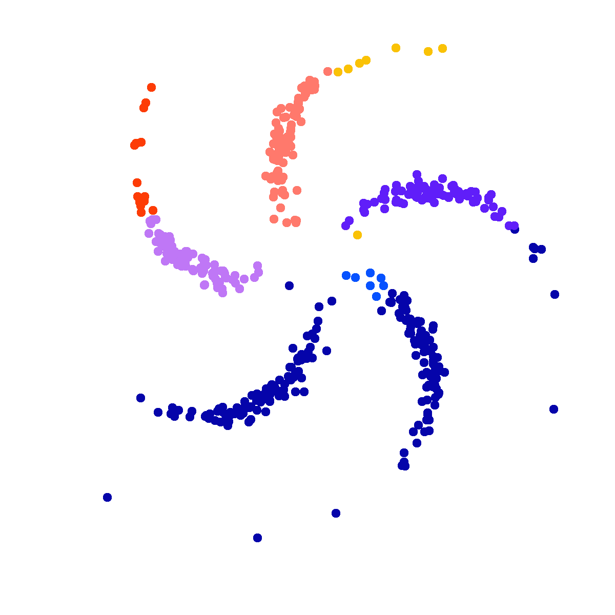
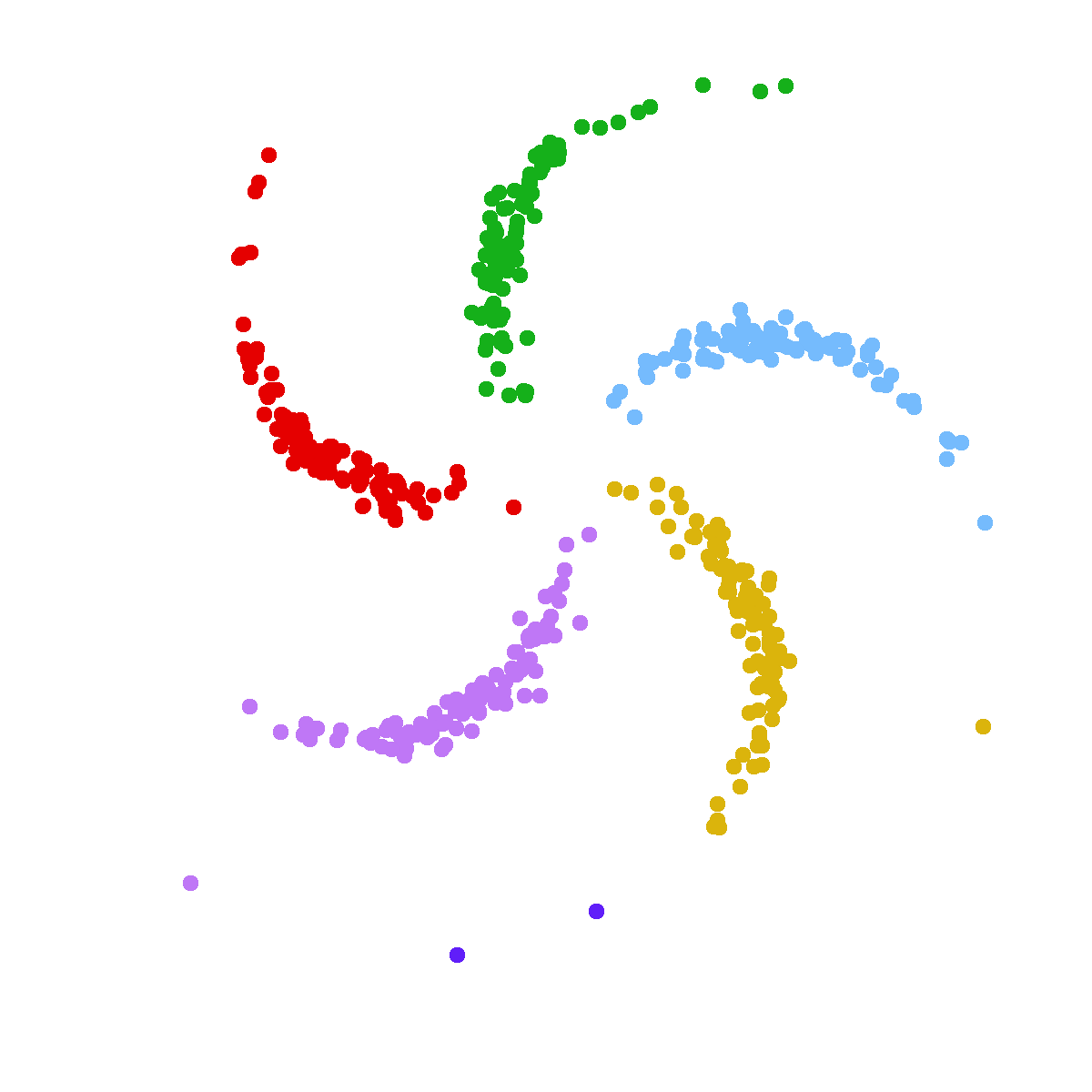
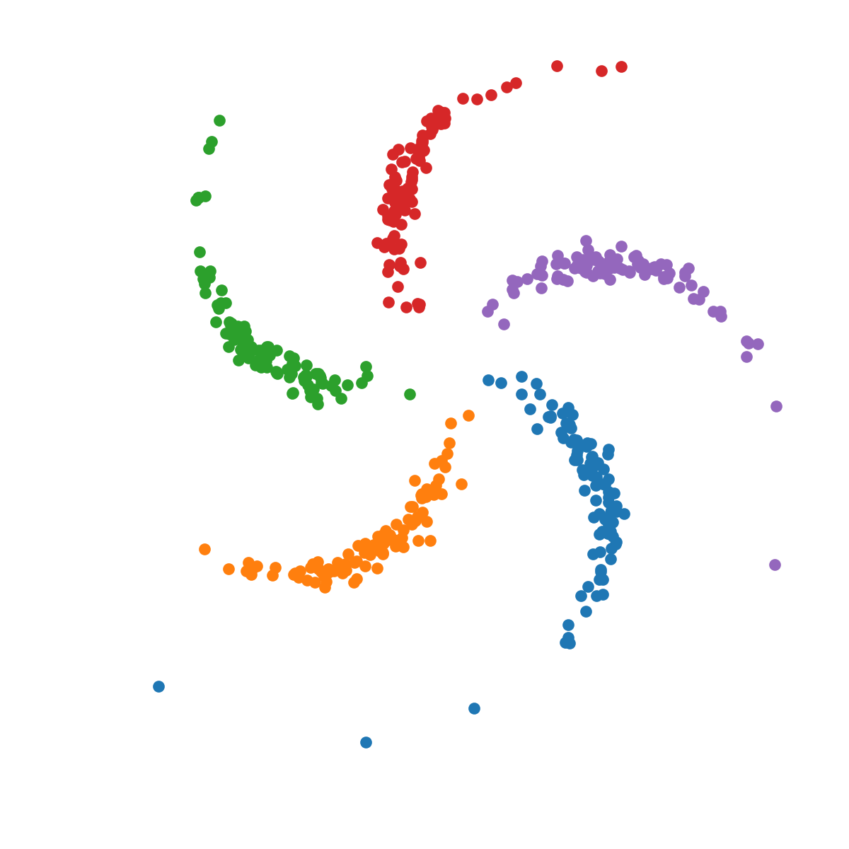
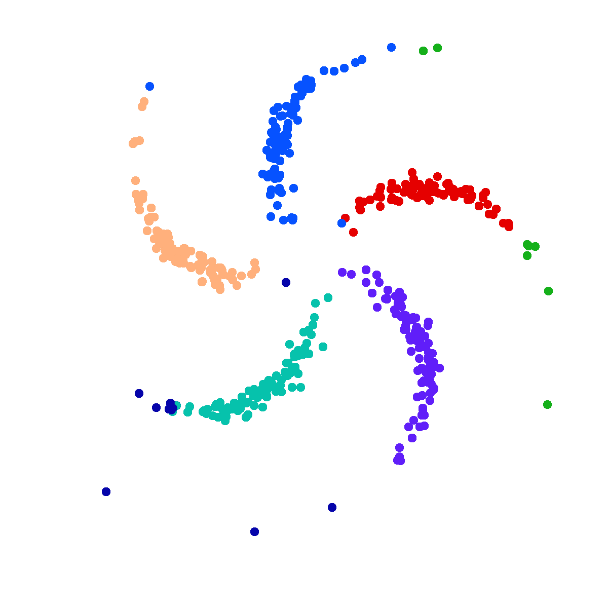
Figure 2: Clustering results on the Pinwheel dataset, with each color representing one cluster.

First we apply our method to a toy example–the pinwheel dataset in Fig. 2(a) following [13, 16]. It has 5 clusters and each cluster has 100 data points, thus there are 500 data points in total. We compare with unsupervised clustering to understand the help of noisy annotations. The clustering results are shown in Fig. 2. We random sampled 100 data points for annotations and simulate 20 workers, each worker gives 49 pairs of annotations, 980 in total. We set equal accuracy to each worker αm=βm=0.9subscript𝛼𝑚subscript𝛽𝑚0.9\alpha_{m}=\beta_{m}=0.9.

We use the fully Bayesian model (BayesSCDC) described in Section 3. The initial number of clusters is set to a larger number K=15𝐾15K=15 since the hyper priors have sparsity property intrinsically and can learn the number of clusters automatically. Unsupervised clustering is sensitive to the initializations, which achieves 95.6% accuracy and NMI score 0.91 with good initializations as shown in Fig. 2(b). After training, it learns K=8𝐾8K=8 clusters. However, with bad initializations, the accuracy and NMI score of unsupervised clustering are 75.6% and 0.806, respectively, as shown in Fig. 2(c). With noisy annotations on random sampled 100 data points, our model improves accuracy to 96.6% and NMI score to 0.94. And it converges to K=6𝐾6K=6 clusters. Our model prevents the bad results in Fig. 2(c) by making use of annotations.

5.2 UCI benchmark experiments

In this subsection, we compare the proposed SCDC with the competing methods on the UCI benchmarks. The baselines include MCVC [3], SemiCrowd [30], semi-supervised clustering methods such as ITML [4], MPCKMeans [1] and Cluster-based Similarity Partitioning Algorithm (CSPA[22].

Crowdsourced annotations are not available for UCI datasets. Following the experimental protocol in MCVC [3], we generate noisy annotations given by M=5𝑀5M=5 simulated workers with different sensitivity and specificity, i.e., 𝜶=𝜷=[0.95,0.9,0.85,0.8,0.75]𝜶𝜷0.950.90.850.80.75{\bm{\alpha}}={\bm{\beta}}=[0.95,0.9,0.85,0.8,0.75], which is more challenging than equal accuracy parameters. The annotations provided by each worker varies from 200200200 to 200020002000 and the number of ML constraints equals to the number of CL constraints.

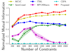
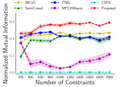
We test on Face dataset [7], containing 640 face images from 20 people with different poses (straight, left, right, up). The ground-truth clustering is based on the poses. The original image has 960 pixels. To speed up training, baseline methods apply Principle Component Analysis (PCA) and keep 20 components. For fair comparison, we test the proposed SCDC on the features after PCA. Fig. 3 plots the mean and standard deviation of NMI scores in 10 different runs for each fixed number of constraints. In Fig. 3(a), the annotations are randomly generated on the whole dataset. We observe that our method consistently outperforms all competing methods, demonstrating that the clustering benefits from the joint generative modeling of inputs and annotations.
Refer to caption
(a)
Refer to caption
(b)
Refer to caption
(c)
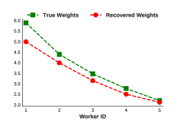
Figure 3: Comparison to baselines: (a) Face: All the data points are annotated; (b) Face: Only 100 data points are annotated; (c) True accuracies are set to 𝜶=𝜷=[0.95,0.9,0.85,0.8,0.75]𝜶𝜷0.950.90.850.80.75{\bm{\alpha}}={\bm{\beta}}=[0.95,0.9,0.85,0.8,0.75]. The green line is the true weights of each worker and the red line is the estimated weights by our model.

Annotations on a subset. To illustrate the benefits of our method in the situation where only a small part of data points are annotated, we simulate noisy annotations on only 100 images. Fig. 3(b) shows the results of 100 annotated images. Our method exploits more structure information in the unlabeled data and shows notable improvements over all competing methods.

Recover worker behaviors. For each worker m𝑚m, our model estimates the different accuracies αmsubscript𝛼𝑚\alpha_{m} and βmsubscript𝛽𝑚\beta_{m}. We can derive from eq. 2 that the annotations of each worker m𝑚m are weighted by logαm1αm+logβm1βmsubscript𝛼𝑚1subscript𝛼𝑚subscript𝛽𝑚1subscript𝛽𝑚\log\frac{\alpha_{m}}{1-\alpha_{m}}+\log\frac{\beta_{m}}{1-\beta_{m}}, which means workers with higher accuracies are more reliable and will be weighted higher. We plot the weights of 5 workers in the Face experiments in Fig. 3(c).

5.3 End-to-end training with raw images

MNIST

As mentioned earlier, an important feature of DGMs is that they can directly model raw data, such as images. To verify this, we experiment with the MNIST dataset of digit images, which includes 60k training images from handwritten digits 0-9. We collect crowdsourced annotations from M=48𝑀48M=48 workers and get 3276 annotations in total. The two variants of our model (SCDC, BayesSCDC) are tested with or without annotations. For BayesSCDC, a non-informative prior Beta(1,1)Beta11\mathrm{Beta}(1,1) is placed over 𝜶,𝜷𝜶𝜷{\bm{\alpha}},{\bm{\beta}}. For fair comparison, we also randomly sample the initial accuracy parameters 𝜶,𝜷𝜶𝜷{\bm{\alpha}},{\bm{\beta}} from Beta(1,1)Beta11\mathrm{Beta}(1,1) for SCDC. We average the results of 5 runs. In each run we randomly initialize the model for 10 times and pick the best result. All models are trained for 200 epochs with minibatch size of 128 for each random initialization. The results are shown in Table 1. We can see that both models can effectively combine the information from the raw data and annotations, i.e., they worked reasonably well with only unlabeled data, and better when given noisy annotations on a subset of data. In terms of clustering accuracy and NMI, BayesSCDC outperforms SCDC. We believe that this is because the variational message passing algorithm used in BayesSCDC can effectively gather information from the crowdsourced annotations to form better variational approximations, as explained in Section 3.2. Besides being more accurate, BayesSCDC is much faster because the computation cost caused by neural networks does not scales linearly with the number of clusters K𝐾K (50 in this case). In Fig. 4(a) we show that BayesSCDC is more flexible and automatically determines the number of mixture components during training.

Table 1: Clustering performance on MNIST. The average time per epoch is reported.
Method without annotations with annotations
Accuracy NMI Time Accuracy NMI Time
SCDC 65.92 ±plus-or-minus\pm 3.47 % 0.6953 ±plus-or-minus\pm 0.0167 177.3s 81.87 ±plus-or-minus\pm 3.86% 0.7657 ±plus-or-minus\pm 0.0233 201.7s
BayesSCDC 77.64 ±plus-or-minus\pm 3.97 % 0.7944 ±plus-or-minus\pm 0.0178 11.2s 84.24 ±plus-or-minus\pm 5.52% 0.8120 ±plus-or-minus\pm 0.0210 16.4s
Epoch 1 \addvbuffer[2pt 0pt]Refer to caption
Epoch 7 \addvbuffer[2pt 0pt]Refer to caption
Epoch 25 \addvbuffer[2pt 0pt]Refer to caption
Epoch 200 \addvbuffer[2pt 0pt]Refer to caption
(a)
Refer to caption
Refer to caption
(b)
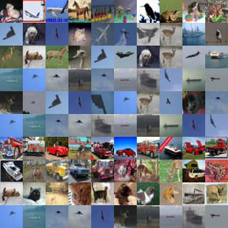
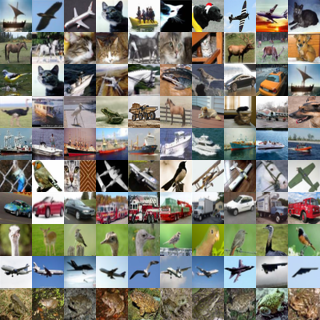
Figure 4: (a) MNIST: visualization of generated random samples of 50 clusters during training BayesSCDC. Each column represents a cluster, whose inferred proportion (πksubscript𝜋𝑘\pi_{k}) is reflected by brightness; (b) Clustering results on CIFAR-10: (top) unsupervised; (bottom) with noisy annotations.

CIFAR-10

We also conduct experiments with real crowdsourced labels on more complex natural images, i.e., CIFAR-10. Using the same crowdsourcing scheme, we collect 8640 noisy annotations from 32 web workers on a subset of randomly sampled 4000 images. We apply SCDC with/without annotations for 5 runs of random initializations. SCDC without annotations failed with NMI score 0.0424 ±plus-or-minus\pm 0.0119 and accuracy 14.23 ±plus-or-minus\pm 0.69% among 5 runs. But the NMI score achieved by SCDC with noisy annotations is 0.5549 ±plus-or-minus\pm 0.0028 and the accuracy is 50.09 ±plus-or-minus\pm 0.08%. The clustering results on test dataset are shown in Fig. 4(b). We plot 10 test samples with the largest probability for each cluster. More experiment details and discussions could be found in the supplementary material.

6 Conclusion

In this paper, we proposed a semi-crowdsourced clustering model based on deep generative models and its fully Bayesian version. We developed fast (natural-gradient) stochastic variational inference algorithms for them. The resulting method can jointly model the crowdsourced labels, worker behaviors, and the (un)annotated items. Experiments have demonstrated that the proposed method outperforms previous competing methods on standard benchmark datasets. Our work also provides general guidelines on how to incorporate DGMs to statistical relational models, where the proposed inference algorithm can be applied under a broader context.

Acknowledgement

Yucen Luo would like to thank Matthew Johnson for helpful discussions on the SVAE algorithm [13], and Yale Chang for sharing the code of the UCI benchmark experiments. We thank the anonymous reviewers for feedbacks that greatly improved the paper. This work was supported by the National Key Research and Development Program of China (No. 2017YFA0700904), NSFC Projects (Nos. 61620106010, 61621136008, 61332007), Beijing NSF Project (No. L172037), Tiangong Institute for Intelligent Computing, NVIDIA NVAIL Program, and the projects from Siemens, NEC and Intel.

References

  • [1] Mikhail Bilenko, Sugato Basu, and Raymond J Mooney. Integrating constraints and metric learning in semi-supervised clustering. In Proceedings of the twenty-first international conference on Machine learning, page 11. ACM, 2004.
  • [2] Varun Chandola, Arindam Banerjee, and Vipin Kumar. Anomaly detection: A survey. ACM computing surveys (CSUR), 41(3):15, 2009.
  • [3] Yale Chang, Junxiang Chen, Michael H Cho, Peter J Castaldi, Edwin K Silverman, and Jennifer G Dy. Multiple clustering views from multiple uncertain experts. In International Conference on Machine Learning, pages 674–683, 2017.
  • [4] Jason V Davis, Brian Kulis, Prateek Jain, Suvrit Sra, and Inderjit S Dhillon. Information-theoretic metric learning. In Proceedings of the 24th international conference on Machine learning, pages 209–216. ACM, 2007.
  • [5] Alexander Philip Dawid and Allan M Skene. Maximum likelihood estimation of observer error-rates using the em algorithm. Applied Statistics, pages 20–28, 1979.
  • [6] Jia Deng, Wei Dong, Richard Socher, Li-Jia Li, Kai Li, and Li Fei-Fei. Imagenet: A large-scale hierarchical image database. In Computer Vision and Pattern Recognition, 2009. CVPR 2009. IEEE Conference on, pages 248–255. IEEE, 2009.
  • [7] Dua Dheeru and Efi Karra Taniskidou. UCI machine learning repository, 2017.
  • [8] Ryan G Gomes, Peter Welinder, Andreas Krause, and Pietro Perona. Crowdclustering. In Advances in neural information processing systems, pages 558–566, 2011.
  • [9] Prem K Gopalan, Sean Gerrish, Michael Freedman, David M Blei, and David M Mimno. Scalable inference of overlapping communities. In Advances in Neural Information Processing Systems, pages 2249–2257, 2012.
  • [10] Kaiming He, Xiangyu Zhang, Shaoqing Ren, and Jian Sun. Deep residual learning for image recognition. In Proceedings of the IEEE conference on computer vision and pattern recognition, pages 770–778, 2016.
  • [11] Matthew D Hoffman, David M Blei, Chong Wang, and John Paisley. Stochastic variational inference. The Journal of Machine Learning Research, 14(1):1303–1347, 2013.
  • [12] Jeff Howe. The rise of crowdsourcing. Wired magazine, 14(6):1–4, 2006.
  • [13] Matthew Johnson, David K Duvenaud, Alex Wiltschko, Ryan P Adams, and Sandeep R Datta. Composing graphical models with neural networks for structured representations and fast inference. In Advances in neural information processing systems, pages 2946–2954, 2016.
  • [14] Diederik P Kingma, Shakir Mohamed, Danilo Jimenez Rezende, and Max Welling. Semi-supervised learning with deep generative models. In Advances in Neural Information Processing Systems, pages 3581–3589, 2014.
  • [15] Diederik P Kingma and Max Welling. Auto-encoding variational bayes. arXiv preprint arXiv:1312.6114, 2013.
  • [16] Wu Lin, Mohammad Emtiyaz Khan, and Nicolas Hubacher. Variational message passing with structured inference networks. In International Conference on Learning Representations, 2018.
  • [17] Yucen Luo, Jun Zhu, Mengxi Li, Yong Ren, and Bo Zhang. Smooth neighbors on teacher graphs for semi-supervised learning. In The IEEE Conference on Computer Vision and Pattern Recognition, 2018.
  • [18] V. C. Raykar, S. Yu, L. H. Zhao, G. H. Valadez, C. Florin, L. Bogoni, and L. Moy. Learning from crowds. JMLR, 11:1297–1322, 2010.
  • [19] Danilo J Rezende, Shakir Mohamed, Ivo Danihelka, Karol Gregor, and Daan Wierstra. One-shot generalization in deep generative models. In Proceedings of the 33rd International Conference on International Conference on Machine Learning-Volume 48, pages 1521–1529. JMLR. org, 2016.
  • [20] Jianbo Shi and Jitendra Malik. Normalized cuts and image segmentation. IEEE Transactions on pattern analysis and machine intelligence, 22(8):888–905, 2000.
  • [21] Jiaxin Shi, Jianfei. Chen, Jun Zhu, Shengyang Sun, Yucen Luo, Yihong Gu, and Yuhao Zhou. ZhuSuan: A library for Bayesian deep learning. arXiv preprint arXiv:1709.05870, 2017.
  • [22] Alexander Strehl and Joydeep Ghosh. Cluster ensembles—a knowledge reuse framework for combining multiple partitions. Journal of machine learning research, 3(Dec):583–617, 2002.
  • [23] Tian Tian and Jun Zhu. Max-margin majority voting for learning from crowds. In Advances in Neural Information Processing Systems, pages 1621–1629, 2015.
  • [24] Ramya Korlakai Vinayak and Babak Hassibi. Crowdsourced clustering: Querying edges vs triangles. In Neural Information Processing System, 2016.
  • [25] Peter Welinder, Steve Branson, Pietro Perona, and Serge J Belongie. The multidimensional wisdom of crowds. In Advances in neural information processing systems, pages 2424–2432, 2010.
  • [26] John Winn and Christopher M Bishop. Variational message passing. Journal of Machine Learning Research, 6(Apr):661–694, 2005.
  • [27] Christian Wiwie, Jan Baumbach, and Richard Röttger. Comparing the performance of biomedical clustering methods. Nature methods, 12(11):1033–1038, 2015.
  • [28] Junyuan Xie, Ross Girshick, and Ali Farhadi. Unsupervised deep embedding for clustering analysis. In International conference on machine learning, pages 478–487, 2016.
  • [29] Eric P Xing, Michael I Jordan, Stuart J Russell, and Andrew Y Ng. Distance metric learning with application to clustering with side-information. In Advances in neural information processing systems, pages 521–528, 2003.
  • [30] Jinfeng Yi, Rong Jin, Shaili Jain, Tianbao Yang, and Anil K Jain. Semi-crowdsourced clustering: Generalizing crowd labeling by robust distance metric learning. In Advances in neural information processing systems, pages 1772–1780, 2012.
  • [31] Dengyong Zhou, Qiang Liu, John Platt, and Christopher Meek. Aggregating ordinal labels from crowds by minimax conditional entropy. In Proceedings of the 31th International Conference on Machine Learning, ICML 2014, Beijing, China, 21-26 June 2014, pages 262–270, 2014.

Appendix A Derivations

A.1 Natural parameters and sufficient statistics

𝜼𝝅=[α11αK1],𝜼𝐳(𝝅)=[logπ1logπK],(𝜼𝝁,𝚺)(k)=[κ𝐦vec(𝐒+κ𝐦𝐦)κν+d+2],𝜼𝐱(𝝁,𝚺)=[𝚺1𝝁vec(12𝚺1)].formulae-sequencesubscript𝜼𝝅matrixsubscript𝛼11subscript𝛼𝐾1formulae-sequencesubscript𝜼𝐳𝝅matrixsubscript𝜋1subscript𝜋𝐾formulae-sequencesuperscriptsubscript𝜼𝝁𝚺𝑘matrix𝜅𝐦vec𝐒𝜅superscript𝐦𝐦top𝜅𝜈𝑑2subscript𝜼𝐱𝝁𝚺matrixsuperscript𝚺1𝝁vec12superscript𝚺1{\bm{\eta}}_{{\bm{\pi}}}=\begin{bmatrix}\alpha_{1}-1\\ \vdots\\ \alpha_{K}-1\end{bmatrix},{\bm{\eta}}_{\mathbf{z}}({\bm{\pi}})=\begin{bmatrix}\log\pi_{1}\\ \vdots\\ \log\pi_{K}\end{bmatrix},({\bm{\eta}}_{{\bm{\mu}},{\bm{\Sigma}}})^{(k)}=\begin{bmatrix}\kappa\mathbf{m}\\ \mathrm{vec}(\mathbf{S}+\kappa\mathbf{m}\mathbf{m}^{\top})\\ \kappa\\ \nu+d+2\end{bmatrix},{\bm{\eta}}_{\mathbf{x}}({\bm{\mu}},{\bm{\Sigma}})=\begin{bmatrix}{\bm{\Sigma}}^{-1}{\bm{\mu}}\\ \mathrm{vec}(-\frac{1}{2}{\bm{\Sigma}}^{-1})\end{bmatrix}.
𝐭(𝝅)=[logπ1logπK],𝐭(𝐳)=[z1zK],𝐭(𝝁,𝚺)(k)=[𝚺k1𝝁kvec(12𝚺k1)12𝝁k𝚺k1𝝁k12ln|𝚺k|],𝐭(𝐱)=[𝐱vec(𝐱𝐱)].formulae-sequence𝐭𝝅matrixsubscript𝜋1subscript𝜋𝐾formulae-sequence𝐭𝐳matrixsubscript𝑧1subscript𝑧𝐾formulae-sequence𝐭superscript𝝁𝚺𝑘matrixsuperscriptsubscript𝚺𝑘1subscript𝝁𝑘vec12superscriptsubscript𝚺𝑘112superscriptsubscript𝝁𝑘topsuperscriptsubscript𝚺𝑘1subscript𝝁𝑘12subscript𝚺𝑘𝐭𝐱matrix𝐱vecsuperscript𝐱𝐱top\mathbf{t}({\bm{\pi}})=\begin{bmatrix}\log\pi_{1}\\ \vdots\\ \log\pi_{K}\end{bmatrix},\mathbf{t}(\mathbf{z})=\begin{bmatrix}z_{1}\\ \vdots\\ z_{K}\end{bmatrix},\mathbf{t}({\bm{\mu}},{\bm{\Sigma}})^{(k)}=\begin{bmatrix}{\bm{\Sigma}}_{k}^{-1}{\bm{\mu}}_{k}\\ \mathrm{vec}{(-\frac{1}{2}{\bm{\Sigma}}_{k}^{-1})}\\ -\frac{1}{2}{\bm{\mu}}_{k}^{\top}{\bm{\Sigma}}_{k}^{-1}{\bm{\mu}}_{k}\\ -\frac{1}{2}\ln|{\bm{\Sigma}}_{k}|\end{bmatrix},\mathbf{t}(\mathbf{x})=\begin{bmatrix}\mathbf{x}\\ \mathrm{vec}(\mathbf{x}\mathbf{x}^{\top})\end{bmatrix}.
(𝜼𝜶)(m)=[ταm11ταm21],𝐭(𝜶)(m)=[logαmlog(1αm)],𝜼𝜷 and 𝐭(𝜷) are similar.formulae-sequencesuperscriptsubscript𝜼𝜶𝑚matrixsubscript𝜏superscriptsubscript𝛼𝑚11subscript𝜏superscriptsubscript𝛼𝑚21𝐭superscript𝜶𝑚matrixsubscript𝛼𝑚1subscript𝛼𝑚𝜼𝜷 and 𝐭(𝜷) are similar.({\bm{\eta}}_{{\bm{\alpha}}})^{(m)}=\begin{bmatrix}\tau_{\alpha_{m}^{1}}-1\\ \tau_{\alpha_{m}^{2}}-1\end{bmatrix},\quad\mathbf{t}({\bm{\alpha}})^{(m)}=\begin{bmatrix}\log\alpha_{m}\\ \log(1-\alpha_{m})\end{bmatrix},\quad\text{${\bm{\eta}}_{{\bm{\beta}}}$ and $\mathbf{t}({\bm{\beta}})$ are similar.}

Note that 𝐭(𝝅)=𝜼𝐳(𝝅)𝐭𝝅subscript𝜼𝐳𝝅\mathbf{t}({\bm{\pi}})={\bm{\eta}}_{\mathbf{z}}({\bm{\pi}}), 𝜼𝐱(𝝁,𝚺)=𝐭(𝝁,𝚺)[:2]{\bm{\eta}}_{\mathbf{x}}({\bm{\mu}},{\bm{\Sigma}})=\mathbf{t}({\bm{\mu}},{\bm{\Sigma}})[:2], where the conjugacy comes. In practice, we parameterized the unnormalized version of 𝜼𝐳~(𝝅)=[logπ1+clogπK+c],~subscript𝜼𝐳𝝅matrixsubscript𝜋1𝑐subscript𝜋𝐾𝑐\tilde{{\bm{\eta}}_{\mathbf{z}}}({\bm{\pi}})=\begin{bmatrix}\log\pi_{1}+c\\ \vdots\\ \log\pi_{K}+c\end{bmatrix}, since it is unconstrained. The update rule for 𝜼𝐳~(𝝅)~subscript𝜼𝐳𝝅\tilde{{\bm{\eta}}_{\mathbf{z}}}({\bm{\pi}}) is the same with 𝜼𝐳(𝝅)subscript𝜼𝐳𝝅{\bm{\eta}}_{\mathbf{z}}({\bm{\pi}}) due to their constant difference.

A.2 Expected sufficient statistics

𝔼q(𝝅)𝐭(𝝅)=[ψ(α1)ψ(αK)]ψ(k=1Kαk),𝔼q(𝝁,𝚺)𝐭(𝝁,𝚺)(k)=[ν𝐒1𝐦vec(12ν𝐒1)12(κ1d+ν𝐦𝐒1𝐦)12(ψd(ν2)+dln2ln|𝐒|)],formulae-sequencesubscript𝔼𝑞𝝅𝐭𝝅matrix𝜓subscript𝛼1𝜓subscript𝛼𝐾𝜓superscriptsubscript𝑘1𝐾subscript𝛼𝑘subscript𝔼𝑞𝝁𝚺𝐭superscript𝝁𝚺𝑘matrix𝜈superscript𝐒1𝐦vec12𝜈superscript𝐒112superscript𝜅1𝑑𝜈superscript𝐦topsuperscript𝐒1𝐦12subscript𝜓𝑑𝜈2𝑑2𝐒\mathbb{E}_{q({\bm{\pi}})}\mathbf{t}({\bm{\pi}})=\begin{bmatrix}\psi(\alpha_{1})\\ \vdots\\ \psi(\alpha_{K})\end{bmatrix}-\psi\left(\sum_{k=1}^{K}\alpha_{k}\right),\quad\mathbb{E}_{q({\bm{\mu}},{\bm{\Sigma}})}\mathbf{t}({\bm{\mu}},{\bm{\Sigma}})^{(k)}=\begin{bmatrix}\nu\mathbf{S}^{-1}\mathbf{m}\\ \mathrm{vec}(-\frac{1}{2}\nu\mathbf{S}^{-1})\\ -\frac{1}{2}(\kappa^{-1}d+\nu\mathbf{m}^{\top}\mathbf{S}^{-1}\mathbf{m})\\ \frac{1}{2}\left(\psi_{d}(\frac{\nu}{2})+d\ln 2-\ln|\mathbf{S}|\right)\end{bmatrix},

where ψd(ν2)=i=1dψ(ν+1i2)subscript𝜓𝑑𝜈2superscriptsubscript𝑖1𝑑𝜓𝜈1𝑖2\psi_{d}(\frac{\nu}{2})=\sum_{i=1}^{d}\psi(\frac{\nu+1-i}{2}), ψ𝜓\psi is the digamma function.

𝔼q(𝐳)𝐭(𝐳)=[π1πK],𝔼q(𝐱)𝐭(𝐱)=[𝝁,vec(𝚺+𝝁𝝁)]formulae-sequencesubscript𝔼𝑞𝐳𝐭𝐳matrixsubscript𝜋1subscript𝜋𝐾subscript𝔼𝑞𝐱𝐭𝐱matrix𝝁vec𝚺𝝁superscript𝝁top\mathbb{E}_{q(\mathbf{z})}\mathbf{t}(\mathbf{z})=\begin{bmatrix}\pi_{1}\\ \vdots\\ \pi_{K}\end{bmatrix},\quad\mathbb{E}_{q(\mathbf{x})}\mathbf{t}(\mathbf{x})=\begin{bmatrix}{\bm{\mu}},\\ \mathrm{vec}({\bm{\Sigma}}+{\bm{\mu}}{\bm{\mu}}^{\top})\end{bmatrix}
𝔼q(𝜶)𝐭(𝜶)(m)=[ψ(ταm1)ψ(ταm2)]ψ(ταm1+ταm2),𝔼q(𝜷)𝐭(𝜷) is similar.subscript𝔼𝑞𝜶𝐭superscript𝜶𝑚matrix𝜓subscript𝜏superscriptsubscript𝛼𝑚1𝜓subscript𝜏superscriptsubscript𝛼𝑚2𝜓subscript𝜏superscriptsubscript𝛼𝑚1subscript𝜏superscriptsubscript𝛼𝑚2𝔼q(𝜷)𝐭(𝜷) is similar.\mathbb{E}_{q({\bm{\alpha}})}\mathbf{t}({\bm{\alpha}})^{(m)}=\begin{bmatrix}\psi(\tau_{\alpha_{m}^{1}})\\ \psi(\tau_{\alpha_{m}^{2}})\end{bmatrix}-\psi(\tau_{\alpha_{m}^{1}}+\tau_{\alpha_{m}^{2}}),\quad\text{$\mathbb{E}_{q({\bm{\beta}})}\mathbf{t}({\bm{\beta}})$ is similar.}

A.3 Log partition function

lnZ(𝜼𝝅)=k=1KlnΓ(αk)lnΓ(k=1Kαk),lnZ(𝜼𝝁,𝚺)=ν2(dln2ln|S|)+lnΓd(ν2)d2lnκ,formulae-sequence𝑍subscript𝜼𝝅superscriptsubscript𝑘1𝐾Γsubscript𝛼𝑘Γsuperscriptsubscript𝑘1𝐾subscript𝛼𝑘𝑍subscript𝜼𝝁𝚺𝜈2𝑑2𝑆subscriptΓ𝑑𝜈2𝑑2𝜅\ln Z({\bm{\eta}}_{{\bm{\pi}}})=\sum_{k=1}^{K}\ln\Gamma(\alpha_{k})-\ln\Gamma\left(\sum_{k=1}^{K}\alpha_{k}\right),\quad\ln Z({\bm{\eta}}_{{\bm{\mu}},{\bm{\Sigma}}})=\frac{\nu}{2}(d\ln 2-\ln|S|)+\ln\Gamma_{d}\left(\frac{\nu}{2}\right)-\frac{d}{2}\ln\kappa,

where Γd(ν2)=πd(d1)/4i=1dΓ(ν+1i2)subscriptΓ𝑑𝜈2superscript𝜋𝑑𝑑14superscriptsubscriptproduct𝑖1𝑑Γ𝜈1𝑖2\Gamma_{d}(\frac{\nu}{2})=\pi^{d(d-1)/4}\prod_{i=1}^{d}\Gamma\left(\frac{\nu+1-i}{2}\right), ΓΓ\Gamma is the Gamma function.

lnZ(𝜼𝐳(𝝅))=0,lnZ(𝜼𝐱(𝝁,𝚺))=12(𝝁𝚺1𝝁+ln|𝚺|)=𝟏{𝐭(𝝁,𝚺)[2:]}.\ln Z({\bm{\eta}}_{\mathbf{z}}({\bm{\pi}}))=0,\quad\ln Z({\bm{\eta}}_{\mathbf{x}}({\bm{\mu}},{\bm{\Sigma}}))=\frac{1}{2}\left({\bm{\mu}}^{\top}{\bm{\Sigma}}^{-1}{\bm{\mu}}+\ln|{\bm{\Sigma}}|\right)=-\mathbf{1}^{\top}\{\mathbf{t}({\bm{\mu}},{\bm{\Sigma}})[2:]\}.
lnZ(𝜼𝜶)=lnΓ(τα1)+lnΓ(τα2)lnΓ(τα1+τα2).𝑍subscript𝜼𝜶Γsubscript𝜏superscript𝛼1Γsubscript𝜏superscript𝛼2Γsubscript𝜏superscript𝛼1subscript𝜏superscript𝛼2\ln Z({\bm{\eta}}_{{\bm{\alpha}}})=\ln\Gamma(\tau_{\alpha^{1}})+\ln\Gamma(\tau_{\alpha^{2}})-\ln\Gamma(\tau_{\alpha^{1}}+\tau_{\alpha^{2}}).

A.4 Variational message passing for local parameters

The local update for 𝐱isubscript𝐱𝑖\mathbf{x}_{i}:

𝜼𝐱i=𝔼q(𝝁,𝚺)[𝐭(𝝁,𝚺)[:2]]𝔼q(𝐳i)𝐭(𝐳i)+r(𝐨i;ϕ).{\bm{\eta}}_{\mathbf{x}_{i}}^{*}=\mathbb{E}_{q({\bm{\mu}},{\bm{\Sigma}})}[\mathbf{t}({\bm{\mu}},{\bm{\Sigma}})[:2]]^{\top}\mathbb{E}_{q(\mathbf{z}_{i})}\mathbf{t}(\mathbf{z}_{i})\!+\!r(\mathbf{o}_{i};{\bm{\phi}}). (18)

The local update for 𝐳isubscript𝐳𝑖\mathbf{z}_{i}:

𝜼𝐳i=𝔼q(𝝅)𝐭(𝝅)+𝔼q(𝝁,𝚺)[𝐭(𝝁,𝚺)]𝔼q(𝐱i)[(𝐭(𝐱i),𝟏)]+m=1Mj=1Nwij(m)𝔼q(𝐳j)[𝐭(𝐳j)].superscriptsubscript𝜼subscript𝐳𝑖subscript𝔼𝑞𝝅𝐭𝝅subscript𝔼𝑞𝝁𝚺superscriptdelimited-[]𝐭𝝁𝚺topsubscript𝔼𝑞subscript𝐱𝑖delimited-[]𝐭subscript𝐱𝑖1superscriptsubscript𝑚1𝑀superscriptsubscript𝑗1𝑁superscriptsubscript𝑤𝑖𝑗𝑚subscript𝔼𝑞subscript𝐳𝑗delimited-[]𝐭subscript𝐳𝑗{\bm{\eta}}_{\mathbf{z}_{i}}^{*}=\mathbb{E}_{q({\bm{\pi}})}\mathbf{t}({\bm{\pi}})+\mathbb{E}_{q({\bm{\mu}},{\bm{\Sigma}})}\left[\mathbf{t}({\bm{\mu}},{\bm{\Sigma}})\right]^{\top}\mathbb{E}_{q(\mathbf{x}_{i})}\left[(\mathbf{t}(\mathbf{x}_{i}),\mathbf{1})\right]+\sum_{m\!=\!1}^{M}\sum_{j=1}^{N}w_{ij}^{(m)}\mathbb{E}_{q(\mathbf{z}_{j})}[\mathbf{t}(\mathbf{z}_{j})].

where wij(m)=Iij(m)𝔼q(𝜶,𝜷)[ln1αmβm+Lij(m)(lnαm1αm+lnβm1βm)]superscriptsubscript𝑤𝑖𝑗𝑚superscriptsubscript𝐼𝑖𝑗𝑚subscript𝔼𝑞𝜶𝜷delimited-[]1subscript𝛼𝑚subscript𝛽𝑚superscriptsubscript𝐿𝑖𝑗𝑚subscript𝛼𝑚1subscript𝛼𝑚subscript𝛽𝑚1subscript𝛽𝑚w_{ij}^{(m)}=I_{ij}^{(m)}\mathbb{E}_{q({\bm{\alpha}},{\bm{\beta}})}\left[\ln\frac{1-\alpha_{m}}{\beta_{m}}+L_{ij}^{(m)}\left(\ln\frac{\alpha_{m}}{1-\alpha_{m}}+\ln\frac{\beta_{m}}{1-\beta_{m}}\right)\right].

A.5 The final objective

The final objective:

𝒥(𝜼𝚯;ϕ,𝜸)𝒥subscript𝜼𝚯bold-italic-ϕ𝜸absent\displaystyle\mathcal{J}({\bm{\eta}}_{{\bm{\Theta}}};{\bm{\phi}},{\bm{\gamma}})\triangleq (𝜼𝚯,𝜼𝐙(𝜼𝚯,ϕ),𝜼𝐗(𝜼𝚯,ϕ),𝜸)subscript𝜼𝚯superscriptsubscript𝜼𝐙subscript𝜼𝚯bold-italic-ϕsuperscriptsubscript𝜼𝐗subscript𝜼𝚯bold-italic-ϕ𝜸\displaystyle\leavevmode\nobreak\ \mathcal{L}({\bm{\eta}}_{{\bm{\Theta}}},{\bm{\eta}}_{\mathbf{Z}}^{*}({\bm{\eta}}_{{\bm{\Theta}}},{\bm{\phi}}),{\bm{\eta}}_{\mathbf{X}}^{*}({\bm{\eta}}_{{\bm{\Theta}}},{\bm{\phi}}),{\bm{\gamma}})
=\displaystyle= 𝔼q(𝐗)logp(𝐎|𝐗;𝜸)+𝔼q(𝜶,𝜷)q(𝐙)logp(𝐋(1:M)|𝐙,𝜶,𝜷)subscript𝔼superscript𝑞𝐗𝑝conditional𝐎𝐗𝜸subscript𝔼𝑞𝜶𝜷superscript𝑞𝐙𝑝conditionalsuperscript𝐋:1𝑀𝐙𝜶𝜷\displaystyle\leavevmode\nobreak\ \mathbb{E}_{{q}^{*}\!(\mathbf{X})}\!\log p(\mathbf{O}|\mathbf{X};{\bm{\gamma}})+\mathbb{E}_{q({\bm{\alpha}},{\bm{\beta}}){q}^{*}\!(\mathbf{Z})}\log p(\mathbf{L}^{(1:M)}|\mathbf{Z},{\bm{\alpha}},{\bm{\beta}})
𝔼q(𝝅,𝝁,𝚺)KL(q(𝐙)q(𝐗)p(𝐙|𝝅)p(𝐗|𝝁,𝚺,𝐙))\displaystyle-\mathbb{E}_{q({\bm{\pi}},{\bm{\mu}},{\bm{\Sigma}})}\operatorname{KL}({q}^{*}\!(\mathbf{Z}){q}^{*}\!(\mathbf{X})\|p(\mathbf{Z}|{\bm{\pi}})p(\mathbf{X}|{\bm{\mu}},{\bm{\Sigma}},\mathbf{Z}))
KL(q(𝝅,𝝁,𝚺,𝜶,𝜷)p(𝝅,𝝁,𝚺,𝜶,𝜷)).KLconditional𝑞𝝅𝝁𝚺𝜶𝜷𝑝𝝅𝝁𝚺𝜶𝜷\displaystyle-\operatorname{KL}(q({\bm{\pi}},{\bm{\mu}},{\bm{\Sigma}},{\bm{\alpha}},{\bm{\beta}})\|p({\bm{\pi}},{\bm{\mu}},{\bm{\Sigma}},{\bm{\alpha}},{\bm{\beta}})). (19)

The annotation likelihood term:

𝔼q(𝜶,𝜷)q(𝐙)logp(𝐋(1:M)|𝐙,𝜶,𝜷)=subscript𝔼𝑞𝜶𝜷superscript𝑞𝐙𝑝conditionalsuperscript𝐋:1𝑀𝐙𝜶𝜷absent\displaystyle\mathbb{E}_{q({\bm{\alpha}},{\bm{\beta}})q^{*}(\mathbf{Z})}\log p(\mathbf{L}^{(1:M)}|\mathbf{Z},{\bm{\alpha}},{\bm{\beta}})=
m=1M1i<jN[wij(m)𝔼q(𝐳i)[𝐭(𝐳i)]𝔼q(𝐳j)𝐭(𝐳j)+Iij(m)𝔼q(𝜷)(Lij(m)ln1βmβm+lnβm)].superscriptsubscript𝑚1𝑀subscript1𝑖𝑗𝑁delimited-[]superscriptsubscript𝑤𝑖𝑗𝑚subscript𝔼𝑞subscript𝐳𝑖superscriptdelimited-[]𝐭subscript𝐳𝑖topsubscript𝔼𝑞subscript𝐳𝑗𝐭subscript𝐳𝑗superscriptsubscript𝐼𝑖𝑗𝑚subscript𝔼𝑞𝜷superscriptsubscript𝐿𝑖𝑗𝑚1subscript𝛽𝑚subscript𝛽𝑚subscript𝛽𝑚\displaystyle\quad\sum_{m=1}^{M}\sum_{1\leq i<j\leq N}\left[w_{ij}^{(m)}\mathbb{E}_{q(\mathbf{z}_{i})}[\mathbf{t}(\mathbf{z}_{i})]^{\top}\mathbb{E}_{q(\mathbf{z}_{j})}\mathbf{t}(\mathbf{z}_{j})+I_{ij}^{(m)}\mathbb{E}_{q({\bm{\beta}})}\left(L_{ij}^{(m)}\ln\frac{1-\beta_{m}}{\beta_{m}}+\ln\beta_{m}\right)\right]. (20)

The local KL divergence term:

𝔼q(𝝅,𝝁,𝚺)KL(q(𝐙)q(𝐗)p(𝐙|𝝅)p(𝐗|𝝁,𝚺,𝐙))\displaystyle\leavevmode\nobreak\ \mathbb{E}_{q({\bm{\pi}},{\bm{\mu}},{\bm{\Sigma}})}\operatorname{KL}({q}^{*}\!(\mathbf{Z}){q}^{*}\!(\mathbf{X})\|p(\mathbf{Z}|{\bm{\pi}})p(\mathbf{X}|{\bm{\mu}},{\bm{\Sigma}},\mathbf{Z}))
=𝔼q(𝝅)KL(q(𝐙)p(𝐙|𝝅))+𝔼q(𝝁,𝚺)q(𝐙)KL(q(𝐗)p(𝐗|𝝁,𝚺,𝐙))\displaystyle=\leavevmode\nobreak\ \mathbb{E}_{q({\bm{\pi}})}\mathrm{KL}(q^{*}(\mathbf{Z})\|p(\mathbf{Z}|{\bm{\pi}}))+\mathbb{E}_{q({\bm{\mu}},{\bm{\Sigma}})q^{*}(\mathbf{Z})}\mathrm{KL}(q^{*}(\mathbf{X})\|p(\mathbf{X}|{\bm{\mu}},{\bm{\Sigma}},\mathbf{Z}))
=i=1N{𝔼q(𝝅)KL(q(𝐳i)p(𝐳i|𝝅))+𝔼q(𝝁,𝚺)q(𝐳i)KL(q(𝐱i)p(𝐱i|𝝁,𝚺,𝐳i))}.\displaystyle=\leavevmode\nobreak\ \sum_{i=1}^{N}\left\{\mathbb{E}_{q({\bm{\pi}})}\mathrm{KL}(q^{*}(\mathbf{z}_{i})\|p(\mathbf{z}_{i}|{\bm{\pi}}))+\mathbb{E}_{q({\bm{\mu}},{\bm{\Sigma}})q^{*}(\mathbf{z}_{i})}\mathrm{KL}(q^{*}(\mathbf{x}_{i})\|p(\mathbf{x}_{i}|{\bm{\mu}},{\bm{\Sigma}},\mathbf{z}_{i}))\right\}. (21)
KL(q(𝐳i)p(𝐳i|𝝅))\displaystyle\mathrm{KL}(q^{*}(\mathbf{z}_{i})\|p(\mathbf{z}_{i}|{\bm{\pi}})) =𝜼𝐳i𝜼𝐳i(𝝅),𝔼q(𝐳i)𝐭(𝐳i)absentsuperscriptsubscript𝜼subscript𝐳𝑖subscript𝜼subscript𝐳𝑖𝝅subscript𝔼superscript𝑞subscript𝐳𝑖𝐭subscript𝐳𝑖\displaystyle=\langle{\bm{\eta}}_{\mathbf{z}_{i}}^{*}-{\bm{\eta}}_{\mathbf{z}_{i}}({\bm{\pi}}),\mathbb{E}_{q^{*}(\mathbf{z}_{i})}\mathbf{t}(\mathbf{z}_{i})\rangle
𝔼q(𝝅)KL(q(𝐳i)p(𝐳i|𝝅))\displaystyle\mathbb{E}_{q({\bm{\pi}})}\mathrm{KL}(q^{*}(\mathbf{z}_{i})\|p(\mathbf{z}_{i}|{\bm{\pi}})) =𝜼𝐳i𝔼q(𝝅)𝐭(𝝅),𝔼q(𝐳i)𝐭(𝐳i).absentsuperscriptsubscript𝜼subscript𝐳𝑖subscript𝔼𝑞𝝅𝐭𝝅subscript𝔼superscript𝑞subscript𝐳𝑖𝐭subscript𝐳𝑖\displaystyle=\langle{\bm{\eta}}_{\mathbf{z}_{i}}^{*}-\mathbb{E}_{q({\bm{\pi}})}\mathbf{t}({\bm{\pi}}),\mathbb{E}_{q^{*}(\mathbf{z}_{i})}\mathbf{t}(\mathbf{z}_{i})\rangle.
KL(q(𝐱i)p(𝐱i|𝝁k,𝚺k))=𝜼𝐱i𝜼𝐱i(𝝁,𝚺)(k),𝔼q(𝐱i)𝐭(𝐱i)[lnZ(𝜼𝐱i)lnZ(𝜼𝐱i(𝝁,𝚺)(k))]\mathrm{KL}(q^{*}(\mathbf{x}_{i})\|p(\mathbf{x}_{i}|{\bm{\mu}}_{k},{\bm{\Sigma}}_{k}))=\langle{\bm{\eta}}_{\mathbf{x}_{i}}^{*}-{\bm{\eta}}_{\mathbf{x}_{i}}({\bm{\mu}},{\bm{\Sigma}})^{(k)},\mathbb{E}_{q^{*}(\mathbf{x}_{i})}\mathbf{t}(\mathbf{x}_{i})\rangle-\left[\ln Z({\bm{\eta}}_{\mathbf{x}_{i}}^{*})-\ln Z({\bm{\eta}}_{\mathbf{x}_{i}}({\bm{\mu}},{\bm{\Sigma}})^{(k)})\right] (22)
𝔼q(𝝁,𝚺)q(𝐳i)KL(q(𝐱i)p(𝐱i|𝝁,𝚺,𝐳i))=\displaystyle\mathbb{E}_{q({\bm{\mu}},{\bm{\Sigma}})q^{*}(\mathbf{z}_{i})}\mathrm{KL}(q^{*}(\mathbf{x}_{i})\|p(\mathbf{x}_{i}|{\bm{\mu}},{\bm{\Sigma}},\mathbf{z}_{i}))= 𝜼𝐱i𝔼q(𝝁,𝚺)[𝜼𝐱i(𝝁,𝚺)]𝔼q(𝐳i)𝐭(𝐳i),𝔼q(𝐱i)𝐭(𝐱i)superscriptsubscript𝜼subscript𝐱𝑖subscript𝔼𝑞𝝁𝚺superscriptdelimited-[]subscript𝜼subscript𝐱𝑖𝝁𝚺topsubscript𝔼superscript𝑞subscript𝐳𝑖𝐭subscript𝐳𝑖subscript𝔼superscript𝑞subscript𝐱𝑖𝐭subscript𝐱𝑖\displaystyle\langle{\bm{\eta}}_{\mathbf{x}_{i}}^{*}-\mathbb{E}_{q({\bm{\mu}},{\bm{\Sigma}})}[{\bm{\eta}}_{\mathbf{x}_{i}}({\bm{\mu}},{\bm{\Sigma}})]^{\top}\mathbb{E}_{q^{*}(\mathbf{z}_{i})}\mathbf{t}(\mathbf{z}_{i}),\mathbb{E}_{q^{*}(\mathbf{x}_{i})}\mathbf{t}(\mathbf{x}_{i})\rangle
{lnZ(𝜼𝐱i)𝔼q(𝝁,𝚺)[lnZ(𝜼𝐱i(𝝁,𝚺))]𝔼q(𝐳i)𝐭(𝐳i)}𝑍superscriptsubscript𝜼subscript𝐱𝑖subscript𝔼𝑞𝝁𝚺superscriptdelimited-[]𝑍subscript𝜼subscript𝐱𝑖𝝁𝚺topsubscript𝔼𝑞subscript𝐳𝑖𝐭subscript𝐳𝑖\displaystyle-\left\{\ln Z({\bm{\eta}}_{\mathbf{x}_{i}}^{*})-\mathbb{E}_{q({\bm{\mu}},{\bm{\Sigma}})}[\ln Z({\bm{\eta}}_{\mathbf{x}_{i}}({\bm{\mu}},{\bm{\Sigma}}))]^{\top}\mathbb{E}_{q*(\mathbf{z}_{i})}\mathbf{t}(\mathbf{z}_{i})\right\}
=\displaystyle= 𝜼𝐱i𝔼q(𝝁,𝚺)[𝐭(𝝁,𝚺)[:2]]𝔼q(𝐳i)𝐭(𝐳i),𝔼q(𝐱i)𝐭(𝐱i)\displaystyle\langle{\bm{\eta}}_{\mathbf{x}_{i}}^{*}-\mathbb{E}_{q({\bm{\mu}},{\bm{\Sigma}})}[\mathbf{t}({\bm{\mu}},{\bm{\Sigma}})[:2]]^{\top}\mathbb{E}_{q^{*}(\mathbf{z}_{i})}\mathbf{t}(\mathbf{z}_{i}),\mathbb{E}_{q^{*}(\mathbf{x}_{i})}\mathbf{t}(\mathbf{x}_{i})\rangle
{lnZ(𝜼𝐱i)+𝟏𝔼q(𝝁,𝚺)[𝐭(𝝁,𝚺)[2:]]𝔼q(𝐳i)𝐭(𝐳i)}.\displaystyle-\left\{\ln Z({\bm{\eta}}_{\mathbf{x}_{i}}^{*})+\mathbf{1}^{\top}\mathbb{E}_{q({\bm{\mu}},{\bm{\Sigma}})}[\mathbf{t}({\bm{\mu}},{\bm{\Sigma}})[2:]]^{\top}\mathbb{E}_{q*(\mathbf{z}_{i})}\mathbf{t}(\mathbf{z}_{i})\right\}.

The global KL divergence term:

KL(q(𝝅)p(𝝅))=𝜼𝝅𝜼𝝅0,𝔼q(𝝅)𝐭(𝝅)[lnZ(𝜼𝝅)lnZ(𝜼𝝅0)].KLconditional𝑞𝝅𝑝𝝅subscript𝜼𝝅subscriptsuperscript𝜼0𝝅subscript𝔼𝑞𝝅𝐭𝝅delimited-[]𝑍subscript𝜼𝝅𝑍superscriptsubscript𝜼𝝅0\displaystyle\mathrm{KL}(q({\bm{\pi}})\|p({\bm{\pi}}))=\langle{\bm{\eta}}_{{\bm{\pi}}}-{\bm{\eta}}^{0}_{{\bm{\pi}}},\mathbb{E}_{q({\bm{\pi}})}\mathbf{t}({\bm{\pi}})\rangle-\left[\ln Z({\bm{\eta}}_{{\bm{\pi}}})-\ln Z({\bm{\eta}}_{{\bm{\pi}}}^{0})\right]. (23)
KL(q(𝝁,𝚺)p(𝝁,𝚺))KLconditional𝑞𝝁𝚺𝑝𝝁𝚺\displaystyle\mathrm{KL}(q({\bm{\mu}},{\bm{\Sigma}})\|p({\bm{\mu}},{\bm{\Sigma}})) =k=1K{𝜼𝝁,𝚺(k)𝜼𝝁,𝚺0(k),𝔼q(𝝁,𝚺)𝐭(𝝁,𝚺)(k)\displaystyle=\sum_{k=1}^{K}\left\{{\langle{\bm{\eta}}_{{\bm{\mu}},{\bm{\Sigma}}}}^{(k)}-{{\bm{\eta}}^{0}_{{\bm{\mu}},{\bm{\Sigma}}}}^{(k)},\mathbb{E}_{q({\bm{\mu}},{\bm{\Sigma}})}\mathbf{t}({\bm{\mu}},{\bm{\Sigma}})^{(k)}\rangle\right.
[lnZ(𝜼𝝁,𝚺(k))lnZ(𝜼𝝁,𝚺0(k))]}.\displaystyle\quad-\left.\left[\ln Z({{\bm{\eta}}_{{\bm{\mu}},{\bm{\Sigma}}}}^{(k)})-\ln Z({{\bm{\eta}}_{{\bm{\mu}},{\bm{\Sigma}}}^{0}}^{(k)})\right]\right\}. (24)
KL(q(𝜶)p(𝜶))=𝜼𝜶𝜼𝜶0,𝔼q(𝜶)𝐭(𝜶)[lnZ(𝜼𝜶)lnZ(𝜼𝜶0)],𝜷 is similar.KLconditional𝑞𝜶𝑝𝜶subscript𝜼𝜶subscriptsuperscript𝜼0𝜶subscript𝔼𝑞𝜶𝐭𝜶delimited-[]𝑍subscript𝜼𝜶𝑍superscriptsubscript𝜼𝜶0𝜷 is similar\displaystyle\mathrm{KL}(q({\bm{\alpha}})\|p({\bm{\alpha}}))=\langle{\bm{\eta}}_{{\bm{\alpha}}}-{\bm{\eta}}^{0}_{{\bm{\alpha}}},\mathbb{E}_{q({\bm{\alpha}})}\mathbf{t}({\bm{\alpha}})\rangle-\left[\ln Z({\bm{\eta}}_{{\bm{\alpha}}})-\ln Z({\bm{\eta}}_{{\bm{\alpha}}}^{0})\right],\quad\text{${\bm{\beta}}$ is similar}. (25)

Global variational parameter updates:

~𝜼𝝅𝒥subscript~subscript𝜼𝝅𝒥\displaystyle\tilde{\nabla}_{{\bm{\eta}}_{{\bm{\pi}}}}\mathcal{J} 𝜼𝝅0+i=1N𝔼q(𝐳i)𝐭(𝐳i)𝜼𝝅,absentsuperscriptsubscript𝜼𝝅0superscriptsubscript𝑖1𝑁subscript𝔼𝑞subscript𝐳𝑖𝐭subscript𝐳𝑖subscript𝜼𝝅\displaystyle\approx{\bm{\eta}}_{{\bm{\pi}}}^{0}+\sum_{i=1}^{N}\mathbb{E}_{q(\mathbf{z}_{i})}\mathbf{t}(\mathbf{z}_{i})-{\bm{\eta}}_{{\bm{\pi}}}, (26)
~𝜼𝝁,𝚺𝒥subscript~subscript𝜼𝝁𝚺𝒥\displaystyle\tilde{\nabla}_{{\bm{\eta}}_{{\bm{\mu}},{\bm{\Sigma}}}}\mathcal{J} 𝜼𝝁,𝚺0+i=1N[𝔼q(𝐱i)(𝐭(𝐱i),𝟏)]𝔼q(𝐳i)𝐭(𝐳i)𝜼𝝁,𝚺,absentsuperscriptsubscript𝜼𝝁𝚺0superscriptsubscript𝑖1𝑁superscriptdelimited-[]subscript𝔼𝑞subscript𝐱𝑖𝐭subscript𝐱𝑖1topsubscript𝔼𝑞subscript𝐳𝑖𝐭subscript𝐳𝑖subscript𝜼𝝁𝚺\displaystyle\approx{\bm{\eta}}_{{\bm{\mu}},{\bm{\Sigma}}}^{0}+\sum_{i=1}^{N}\left[\mathbb{E}_{q(\mathbf{x}_{i})}(\mathbf{t}(\mathbf{x}_{i}),\mathbf{1})\right]^{\top}\mathbb{E}_{q(\mathbf{z}_{i})}\mathbf{t}(\mathbf{z}_{i})-{\bm{\eta}}_{{\bm{\mu}},{\bm{\Sigma}}}, (27)
~𝜼𝜶(m)𝒥subscript~superscriptsubscript𝜼𝜶𝑚𝒥\displaystyle\tilde{\nabla}_{{\bm{\eta}}_{{\bm{\alpha}}}^{(m)}}\mathcal{J} =(𝜼𝜶0)(m)+12i,j=1NIij(m)𝔼q(𝐳i)[𝐭(𝐳i)]𝔼q(𝐳j)𝐭(𝐳j)[Lij(m)1Lij(m)]𝜼𝜶(m),absentsuperscriptsuperscriptsubscript𝜼𝜶0𝑚12superscriptsubscript𝑖𝑗1𝑁superscriptsubscript𝐼𝑖𝑗𝑚subscript𝔼𝑞subscript𝐳𝑖superscriptdelimited-[]𝐭subscript𝐳𝑖topsubscript𝔼𝑞subscript𝐳𝑗𝐭subscript𝐳𝑗matrixsubscriptsuperscript𝐿𝑚𝑖𝑗1subscriptsuperscript𝐿𝑚𝑖𝑗superscriptsubscript𝜼𝜶𝑚\displaystyle=({\bm{\eta}}_{{\bm{\alpha}}}^{0})^{(m)}+\frac{1}{2}\sum_{i,j=1}^{N}I_{ij}^{(m)}\mathbb{E}_{q(\mathbf{z}_{i})}[\mathbf{t}(\mathbf{z}_{i})]^{\top}\mathbb{E}_{q(\mathbf{z}_{j})}\mathbf{t}(\mathbf{z}_{j})\begin{bmatrix}L^{(m)}_{ij}\\ 1-L^{(m)}_{ij}\end{bmatrix}-{\bm{\eta}}_{{\bm{\alpha}}}^{(m)}, (28)
~𝜼𝜷(m)𝒥subscript~superscriptsubscript𝜼𝜷𝑚𝒥\displaystyle\tilde{\nabla}_{{\bm{\eta}}_{{\bm{\beta}}}^{(m)}}\mathcal{J} =(𝜼𝜷0)(m)+12i,j=1NIij(m)(1𝔼q(𝐳i)[𝐭(𝐳i)]𝔼q(𝐳j)𝐭(𝐳j))[1Lij(m)Lij(m)]𝜼𝜷(m).absentsuperscriptsuperscriptsubscript𝜼𝜷0𝑚12superscriptsubscript𝑖𝑗1𝑁superscriptsubscript𝐼𝑖𝑗𝑚1subscript𝔼𝑞subscript𝐳𝑖superscriptdelimited-[]𝐭subscript𝐳𝑖topsubscript𝔼𝑞subscript𝐳𝑗𝐭subscript𝐳𝑗matrix1subscriptsuperscript𝐿𝑚𝑖𝑗subscriptsuperscript𝐿𝑚𝑖𝑗superscriptsubscript𝜼𝜷𝑚\displaystyle=({\bm{\eta}}_{{\bm{\beta}}}^{0})^{(m)}+\frac{1}{2}\sum_{i,j=1}^{N}I_{ij}^{(m)}\left(1-\mathbb{E}_{q(\mathbf{z}_{i})}[\mathbf{t}(\mathbf{z}_{i})]^{\top}\mathbb{E}_{q(\mathbf{z}_{j})}\mathbf{t}(\mathbf{z}_{j})\right)\begin{bmatrix}1-L^{(m)}_{ij}\\ L^{(m)}_{ij}\end{bmatrix}-{\bm{\eta}}_{{\bm{\beta}}}^{(m)}. (29)

Appendix B Experiment settings

Toy Pinwheel dataset

We follow the synthetic data generation process and hyperparameter settings in [13]. The latent dim of 𝐱𝐱\mathbf{x} is set to d=2𝑑2d=2 and initial number of clusters K=15𝐾15K=15. The Dirichlet prior for mixing coefficients 𝝅𝝅{\bm{\pi}}: α0=0.05/Ksubscript𝛼00.05𝐾\alpha_{0}=0.05/K. The NIW prior p(𝝁,𝚺)𝑝𝝁𝚺p({\bm{\mu}},{\bm{\Sigma}}): concentration κ=0.5𝜅0.5\kappa=0.5, location parameter 𝒎=𝟎𝒎0\bm{m}=\mathbf{0}, scale matrix 𝐒=(d+κ)𝐈d𝐒𝑑𝜅subscript𝐈𝑑\mathbf{S}=(d+\kappa)\mathbf{I}_{d} (𝐈dd×dsubscript𝐈𝑑superscript𝑑𝑑\mathbf{I}_{d}\in\mathbb{R}^{d\times d} is the identity matrix), degrees of freedom ν=d+κ𝜈𝑑𝜅\nu=d+\kappa. The Beta prior hyperparameter τα01,τα02,τβ01,τβ02subscript𝜏superscriptsubscript𝛼01subscript𝜏superscriptsubscript𝛼02subscript𝜏superscriptsubscript𝛽01subscript𝜏superscriptsubscript𝛽02\tau_{\alpha_{0}^{1}},\tau_{\alpha_{0}^{2}},\tau_{\beta_{0}^{1}},\tau_{\beta_{0}^{2}} for accuracy (𝜶,𝜷)𝜶𝜷({\bm{\alpha}},{\bm{\beta}}) are all set to 1. The hyperparameters in variational distributions of global variables are α0𝒰(1,2),κ=1,𝒎𝒩(0,3),𝐒=(d+κ)𝐈d,ν=d+κ,τα01=τβ01=10,τα02=τβ02=1formulae-sequenceformulae-sequencesimilar-tosubscript𝛼0𝒰12formulae-sequence𝜅1formulae-sequencesimilar-to𝒎𝒩03formulae-sequence𝐒𝑑𝜅subscript𝐈𝑑formulae-sequence𝜈𝑑𝜅subscript𝜏superscriptsubscript𝛼01subscript𝜏superscriptsubscript𝛽0110subscript𝜏superscriptsubscript𝛼02subscript𝜏superscriptsubscript𝛽021\alpha_{0}\sim\mathcal{U}(1,2),\kappa=1,\bm{m}\sim\mathcal{N}(0,3),\mathbf{S}=(d+\kappa)\mathbf{I}_{d},\nu=d+\kappa,\tau_{\alpha_{0}^{1}}=\tau_{\beta_{0}^{1}}=10,\tau_{\alpha_{0}^{2}}=\tau_{\beta_{0}^{2}}=1. The networks of p(𝐨|𝐱;𝜸)𝑝conditional𝐨𝐱𝜸p(\mathbf{o}|\mathbf{x};{\bm{\gamma}}) and recognition networks r(𝐨;ϕ)𝑟𝐨bold-italic-ϕr(\mathbf{o};{\bm{\phi}}) are both MLPs with two hidden layers of 40 ReLU units. The networks are trained for 20 epochs with minibatch size |B|𝐵|B| of 50, momentum 0.9 and learning rate 1×1031superscript1031\times 10^{-3}. The learning rate for global variational parameters 𝜼𝚯subscript𝜼𝚯{\bm{\eta}}_{\bm{\Theta}} is 1×1041superscript1041\times 10^{-4}. The batch size |S|𝑆|S| of annotations is computed by |S|=Na×|B|/N𝑆subscript𝑁𝑎𝐵𝑁|S|=N_{a}\times|B|/N to ensure that the annotations and the images are feed to the network proportionally.

UCI dataset

The implementation of competing methods are based on the source code provided by MCVC [3]. In our proposed SCDC, the preprocessing of images and generation of annotations are the same as that in MCVC. The latent dim is set to d=8𝑑8d=8 and K=4𝐾4K=4. As for the network architecture, p(𝐨|𝐱;𝜸)𝑝conditional𝐨𝐱𝜸p(\mathbf{o}|\mathbf{x};{\bm{\gamma}}) and recognition networks q(𝐳n|𝐨n;ϕ)q(𝐱n|𝐳n,𝐨n;ϕ)𝑞conditionalsubscript𝐳𝑛subscript𝐨𝑛bold-italic-ϕ𝑞conditionalsubscript𝐱𝑛subscript𝐳𝑛subscript𝐨𝑛bold-italic-ϕq(\mathbf{z}_{n}|\mathbf{o}_{n};{\bm{\phi}})q(\mathbf{x}_{n}|\mathbf{z}_{n},\mathbf{o}_{n};{\bm{\phi}}) are simple MLPs with two hidden layers of 40 ReLU units. The networks are trained for 20 epochs using Adam optimizer with learning rate 1×1031superscript1031\times 10^{-3} and batch size |B|=10𝐵10|B|=10 .

MNIST

For both SCDC and BayesSCDC, p(𝐨|𝐱)𝑝conditional𝐨𝐱p(\mathbf{o}|\mathbf{x}) and recognition networks are MLPs with two hidden layers of 500 ReLU units. The latent dim of 𝐱𝐱\mathbf{x} is d=8𝑑8d=8 and initial number of clusters K=50𝐾50K=50. Both two models are trained for 200 epochs. For SCDC, we use Adam optimizer with learning rate 1×1031superscript1031\times 10^{-3} and minibatch size 128. For BayesSCDC, the hyperparameter settings in the priors and variational distributions are all the same as that in the Pinwheel dataset. The networks are trained with minibatch size |B|𝐵|B| of 128, momentum 0.9 and learning rate 1×1031superscript1031\times 10^{-3}.

CIFAR-10

We set latent dim d=64𝑑64d=64 and K=10𝐾10K=10 here. The p(𝐨|𝐱;𝜸)𝑝conditional𝐨𝐱𝜸p(\mathbf{o}|\mathbf{x};{\bm{\gamma}}), q(𝐱|𝐳,𝐨)𝑞conditional𝐱𝐳𝐨q(\mathbf{x}|\mathbf{z},\mathbf{o}) are both parameterized by 5 deep stack of residual blocks [10], making the scale of images changing from 32×32323232\times 32 to 8×8888\times 8 and reversely for q(𝐱|𝐳,𝐨)𝑞conditional𝐱𝐳𝐨q(\mathbf{x}|\mathbf{z},\mathbf{o}). The network of q(𝐳|𝐨)𝑞conditional𝐳𝐨q(\mathbf{z}|\mathbf{o}) is a simple 9-layer convolutional neural networks as adopted by recent deep semi-supervised methods [17]. The networks are trained for 200 epochs with Adam optimizer with learning rate 3×1033superscript1033\times 10^{-3} and minibatch size |B|=100𝐵100|B|=100 and |S|=200𝑆200|S|=200.

Crowdsourcing scheme

For both MNIST and CIFAR-10, we random sample a subset of 4000 images from the training dataset and ask workers on Amazon Mechanical Turks (AMT) to annotate them. In each task, 36 images are sampled from the subset and shown to the worker. Each worker is asked to divide 36 images into any number of clusters. From these feedbacks, we can derive pairwise annotations for following experiments.

Appendix C Addtional experimental results

Comparison with deep MCVC [3]

In Section 5.2, our model performs better than other competing methods because of the generative “instance model" and thus the usage of structure information in unlabeled data. Discriminative methods such as MCVC [3] cannot take advantage of the observations of those unannotated data, even with a more complex deep neural network. For fair comparison, we modify MCVC by using a more complex DNN (abbr. as deep MCVC). We test deep MCVC on the Face dataset, where deep MCVC uses the same network architecture (MLP with two hidden layers of 40 ReLU units) as our q(𝐳|𝐨)𝑞conditional𝐳𝐨q(\mathbf{z}|\mathbf{o}) in our method. As shown in Fig. 5, the performance of deep MCVC is better than MCVC when more constraints are observed but worse than the proposed SCDC. The reason is that deep MCVC does not exploit the information of unannotated images during the training.

Furthermore, we also evaluate deep MCVC on CIFAR-10, whose best NMI score among 5 runs is 0.44. In contrast, the proposed SCDC achieves NMI score 0.55. The gap of the improvement is due to the help of unannotated data.
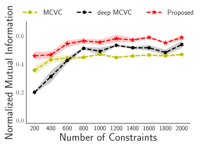
Refer to caption
Figure 5: Comparison to deep MCVC on Face dataset with only a subset of 100 data points annotated. The experiment setting is the same as that in Fig. 3(b).