Sensitivity of $\ell_{1}$ minimization to parameter choice

Abstract

The use of generalized Lasso is a common technique for recovery of structured high-dimensional signals. Each generalized Lasso program has a governing parameter whose optimal value depends on properties of the data. At this optimal value, compressed sensing theory explains why Lasso programs recover structured high-dimensional signals with minimax order-optimal error. Unfortunately in practice, the optimal choice is generally unknown and must be estimated. Thus, we investigate stability of each Lasso program with respect to its governing parameter. Our goal is to aid the practitioner in answering the following question: given real data, which Lasso program should be used? We take a step towards answering this by analyzing the case where the measurement matrix is identity (the so-called proximal denoising setup) and we use $\ell_{1}$ regularization. For each Lasso program, we specify settings in which that program is provably unstable with respect to its governing parameter. We support our analysis with detailed numerical simulations. For example, there are settings where a 0.1% underestimate of a Lasso parameter can increase the error significantly; and a 50% underestimate can cause the error to increase by a factor of $10^{9}$. Parameter instability, Sparse proximal denoising, Lasso, Compressed sensing, Convex optimization

1 Introduction

A fundamental problem of signal processing centers the development and analysis of efficacious methods for structured signal recovery that are widely applicable in practice. Frequently in applications, the signal is assumed to be structured according to some data model and measured by a particular acquisition method. For example, in image deblurring one might assume the objects of interest lie in the dual of a Besov space [28, 24], while in MRI applications, one might assume the images are sparse in a wavelet domain, and measured by subsampling their Fourier coefficients [27]. There is extensive literature concerned with those applications in which the goal is to recover the ground-truth signal from acquired measurements by a prescribed convex program that exploits the signal structure. For example, compressed sensing (CS) has demonstrated that a scale-invariant structure such as sparsity can be captured by convex optimization.

The above paradigm can be put in the following mathematical language. Assume that $K\subseteq\mathbb{R}^{N}$ is a nonempty closed and convex set. Denote the gauge of $K$ by $\|x\|_{K}:=\inf\{\lambda>0:x\in\lambda K\}$ and observe that $\|\cdot\|_{K}$ may be a norm for certain choices of $K$. Assume that a signal $x_{0}\in\mathbb{R}^{N}$ is “structured” in the sense that $\|x_{0}\|_{K}$ is relatively small. Suppose $A\in\mathbb{R}^{m\times N}$ defines the linear measurement process and define the measurements $y=Ax_{0}+\eta z$ where $z\in\mathbb{R}^{m}$ is a possibly stochastic noise vector with noise level $\eta>0$. Here, $1\leq m,N<\infty$ are integers and we do not yet make an assumption on the relative size of $m$ and $N$. For $\tau,\sigma,\lambda>0$, we define the following three generalized Lasso programs, which are convex, where the goal is to best approximate the original signal $x_{0}$.

$$\hat{x}(\tau;y,A,K) :=\operatorname*{\arg\min}\Big{\{}\|y-Ax\|_{2}:x\in\tau K\Big{\}} \mathrm{LS}_{\tau,K}$$ ()

$$x^{\sharp}(\lambda;y,A,K) :=\operatorname*{\arg\min}\Big{\{}\frac{1}{2}\|y-Ax\|_{2}^{2}+\lambda\|x\|_{K}:x\in\mathbb{R}^{N}\Big{\}} \mathrm{QP}_{\lambda,K}$$ ()

$$\tilde{x}(\sigma;y,A,K) :=\operatorname*{\arg\min}\Big{\{}\|x\|_{K}:\|y-Ax\|_{2}\leq\sigma\Big{\}} \mathrm{BP}_{\sigma,K}$$ ()

For brevity of notation, when it is clear from context, we omit explicit dependence of $\hat{x},\tilde{x},x^{\sharp}$ on $y,A$ and $K$. We include below several examples of this general set-up:

1. To obtain total variation (TV) denoising for [continuous-valued discrete] images, define for $x\in\mathbb{R}^{N\times N}$,

   $$\|x\|_{\mathrm{BV}}:=\|x\|_{1}+\sum_{\alpha\in[N]^{2}}\sum_{\beta\in\nu(\alpha)}|x_{\alpha}-x_{\beta}|,$$

   where $[N]=\{1,2,\ldots,N\}$ and $\nu:[N]^{2}\to\mathcal{P}([N]^{2})$ is the neighbour map that determines which “pixels” $x_{\beta}$ of the image are the neighbours of the pixel $x_{\alpha}$. If $\alpha=(i,j)$ and $2\leq i,j\leq N-1$ then one typically has $\nu(i,j)=\{(i-1,j),(i,j-1),(i+1,j),(i,j+1)\}$ with a variety of choices for the remaining indices. So defined, $x^{\sharp}(\lambda;y,I,K)$ is a well-known denoising model for two-dimensional images when $A=I$ is the identity matrix and $K:=\{\|x\|_{\mathrm{BV}}\leq 1\}$ [38]. Instead defining $\|x\|_{\mathrm{BV}}:=\|x\|_{1}+\sum_{i=1}^{N-1}|x_{i+1}-x_{i}|$ for $x\in\mathbb{R}^{N}$, one obtains an equivalent denoising method for one-dimensional signals. With minor modification of $x^{\sharp}(\lambda)$ to allow for $A$ to act as a bounded linear operator on $x\in\mathbb{R}^{N\times N}$ (e.g., convolution with a Gaussian kernel), one may extend the model for image deblurring [15].

2. Say that $x\in\mathbb{R}^{N}$ is $s$-sparse if $x\in\Sigma_{s}^{N}:=\{x\in\mathbb{R}^{N}:\|x\|_{0}\leq s\}$ where $\|x\|_{0}=\#\{j:x_{j}\neq 0\}$. Define $K:=B_{1}^{N}$, suppose $x_{0}\in\mathbb{R}^{N}$ is $s$-sparse for some $s\geq 1$ and suppose that $A\in\mathbb{R}^{m\times N}$ is a Gaussian random matrix with $A_{ij}\overset{\text{iid}}{\sim}\mathcal{N}(0,m^{-1/2})$. Then we obtain three common variants of the Lasso that solve the “vanilla” CS problem: the constrained Lasso yielding $\hat{x}(\tau;y,A,K)$, basis pursuit denoise yielding $\tilde{x}(\sigma;y,A,K)$, and the unconstrained Lasso yielding $x^{\sharp}(\lambda;y,A,K)$.

3. When $A=I$ is the identity matrix, $(\mathrm{LS}_{\tau,K})$ yields the orthogonal projection onto $\tau K$, which we denote by $\mathrm{P}_{\tau K}(y):=\hat{x}(\tau;y,I,K)$. Similarly, $(\mathrm{QP}_{\lambda,K})$ yields the proximal operator for the gauge induced by $K$, which we denote by $\operatorname{\mathrm{prox}}_{\lambda^{-1}K}(y):=x^{\sharp}(\lambda;y,I,K)$. Proximal operators are the workhorses of proximal algorithms. Projected gradient descent methods rely on $\mathrm{P}_{\tau K}(y)$, while $\operatorname{\mathrm{prox}}_{\lambda^{-1}K}(y)$ is central to proximal gradient descent methods.

4. For example, suppose $y=\Phi x_{0}+\eta z$ where $x_{0}$ is $s$-sparse, $\Phi\in\mathbb{R}^{m\times N}$ is a Gaussian random matrix with $m\ll N$ and $\eta z$ is scaled normal random noise. A well-known way of solving for $\hat{x}(\tau;y,\Phi,B_{1}^{N})$ where $B_{1}^{N}$ is the unit $\ell_{1}$ ball, is to compute the following projected gradient descent scheme:

   $$x^{t+1}:=\mathrm{P}_{\tau B_{1}^{N}}(x^{t}-\mu^{t}\nabla\|\Phi x-y\|_{2}^{2}).$$

5. Assume that $x^{\prime}\in\mathbb{R}^{N}$ is $s$-sparse and let $x_{0}=\Psi^{-1}x^{\prime}$ where $\Psi$ is the orthonormal DFT matrix. Given $y=x_{0}+\eta z$, the vector $\hat{x}(\tau;y,\Psi^{-1},B_{1}^{N})$ gives an analogue of running so-called constrained proximal denoising in Fourier space.

6. Consider a matrix $x\in\mathbb{R}^{N\times N}$, let $\|x\|_{*}$ denote its nuclear norm and define $K:=\{x\in\mathbb{R}^{N\times N}:\|x\|_{*}\leq 1\}$. Then $\tilde{x}(\sigma)$ gives the standard optimization program for recovering a low-rank matrix $x_{0}\in\mathbb{R}^{N\times N}$ from measurements $Ax:=\langle A_{i},x\rangle=\sum_{\alpha\in[N]^{2}}A_{i,\alpha}x_{\alpha}$.

In both the second and final examples, the signal $x_{0}$ does not (necessarily) belong to the structure set $K$. Instead, $K$ serves as a kind of structural proxy. To clarify, $K=B_{1}^{N}$ in the second example, which is a structural proxy for sparse vectors in the sense that if $x\in\mathbb{R}^{N}$ is $s$-sparse then $\|x\|_{1}/\|x\|_{2}$ is relatively small compared to non-sparse vectors. A similar statement holds for low-rank matrices and the nuclear norm, as in the final example.

Because of the myriad applications of this class of programs to real-world problems, it is imperative to fully characterize the performance and stability of these algorithms. For example, the error rates of $\hat{x}(\tau)$ are well-known when $\tau$ is equal to the optimal parameter choice, $A$ is a subgaussian random matrix and $K$ is a symmetric, closed, convex set containing the origin [21, 26, 31]. However, the error of the estimator $\hat{x}(\tau)$ is not fully characterized in this setting for values of $\tau$ that are not the optimal choice. Similarly, there lacks a full comparison of the error behaviour between the three estimators $\hat{x}(\tau),\tilde{x}(\sigma)$ and $x^{\sharp}(\lambda)$ as a function of their governing parameters. It is an open question if there are settings in which one estimator is always preferable to another.

Perhaps the most common example of where these programs are used is CS. CS is a provably stable and robust technique for simultaneous data acquisition and dimension reduction [21]. Take the linear measurement model $y=Ax_{0}$, where $x_{0}\in\mathbb{R}^{N}$ is $s$-sparse. The now classical CS result [10, 11, 12, 16, 17, 21] shows if $A$ is suitably random and has $m\geq Cs\log(N/s)$ rows, then one may efficiently recover $x_{0}$ from $(y,A)$. Numerical implementations of CS are commonly tied to one of three convex $\ell_{1}$ programs: constrained Lasso, unconstrained Lasso, and quadratically constrained basis pursuit [40]. The advent of suitable fast and scalable algorithms has made the associated family of convex $\ell_{1}$ minimization problems extremely useful in practice [22, 23, 32, 40].

Proximal Denoising (PD) is a simplification of its more general CS counterpart, in which the measurement matrix is identity. PD uses convex optimization as a means to recover a structured signal corrupted by additive noise. We define three convex programs for PD: constrained proximal denoising, basis pursuit proximal denoising, and unconstrained proximal denoising. To bear greatest relevance to CS, we assume that $x_{0}$ is $s$-sparse, having no more than $s$ non-zero entries, and that $y=x_{0}+\eta z$, where $z\overset{\text{iid}}{\sim}\mathcal{N}(0,1)$ and $\eta>0$. For $\tau,\sigma,\lambda>0$, respectively,

$$\hat{x}(\tau) :=\operatorname*{\arg\min}_{x\in\mathbb{R}^{N}}\big{\{}\|y-x\|_{2}^{2}:\|x\|_{1}\leq\tau\big{\}} \mathrm{LS}_{\tau}^{*}$$ ()

$$\tilde{x}(\sigma) :=\operatorname*{\arg\min}_{x\in\mathbb{R}^{N}}\big{\{}\|x\|_{1}:\|y-x\|_{2}^{2}\leq\sigma^{2}\big{\}} \mathrm{BP}_{\sigma}^{*}$$ ()

$$x^{\sharp}(\lambda) :=\operatorname*{\arg\min}_{x\in\mathbb{R}^{N}}\big{\{}\frac{1}{2}\|y-x\|_{2}^{2}+\lambda\|x\|_{1}\big{\}}. \mathrm{QP}_{\lambda}^{*}$$ ()

These are clear simplifications of $(\mathrm{LS}_{\tau,K})$, $(\mathrm{QP}_{\lambda,K})$ and $(\mathrm{BP}_{\sigma,K})$ introduced above, in which $K=B_{1}^{N}$ is the $\ell_{1}$ ball and where we use ^∗ to denote that the measurement matrix $A\in\mathbb{R}^{N\times N}$ is identity.

Following the dicussion above, minimax order-optimal recovery results for CS and PD programs rely on the ability to make a specific choice of the program’s governing parameter (i.e., “using an oracle”) [21]. However, the optimal choice of the governing parameter for these programs is generally unknown in practice. Consequently, it is desirable that the error of the solution exhibit stability with respect to variation of the parameter about its optimal setting. If the optimal choice of parameter yields order-optimal recovery error, then one may hope that a “nearly” optimal choice of parameter admits “nearly” order-optimal recovery error, too, in the sense that the discrepancy in error is no greater than a multiplicative constant that depends smoothly on the discrepancy in parameter choice. For example, if $R(\alpha)$ is the mean-squared error of a convex program with parameter $\alpha>0$, and $\alpha^{*}>0$ is the value yielding minimal error, then one may hope for smooth dependence on $\alpha$, such as

$$R(\alpha)\lesssim A(\alpha)R(\alpha^{*}),$$

where $A:\mathbb{R}\to\mathbb{R}^{+}$ is a nonnegative smooth function with $A(\alpha^{*})=1$. For example, the risk for $(\mathrm{QP}_{\lambda}^{*})$ satisfies this expression with $A(\lambda)=(\lambda/\lambda^{*})^{2}$ when $\lambda\geq\lambda^{*}$.

Unfortunately, such a hope cannot be guaranteed in general. We prove the existence of regimes in which PD programs exhibit parameter instability — small changes in parameter values can lead to blow-up in risk. Moreover, since the three versions of PD are equivalent in a sense (cf. Proposition 2.4), one might think it does not matter which to choose in practice. However, in this paper we demonstrate regimes in which one program exhibits parameter instability, while the other two do not. For example, in the very sparse regime, our theory and simulations suggest not to use $(\mathrm{BP}_{\sigma}^{*})$, while in the low-noise regime, they suggest not to use $(\mathrm{LS}_{\tau}^{*})$. At the same time, we identify situations where PD programs perform well in theory and simulations alike.

We explore the connection between PD and CS numerically, observing that our theoretical results for PD are mirrored in the CS setup. This holds in both completely synthetic experiments, and for a more realistic example using the Shepp-Logan phantom. Thus, the theoretical results in this paper can help practitioners decide which program to use in CS problems with real data.

2 Summary of results to follow

This section contains three sibling results that simplify the main results in the next sections by considering asymptotic versions of them. By “risk”, we mean the noise-normalized expected squared error (nnse) of an estimator. The risks for the estimators $\hat{x}(\tau),x^{\sharp}(\lambda)$ and $\tilde{x}(\sigma)$ are, respectively:

$$\hat{R}(\tau;x_{0},N,\eta) :=\eta^{-2}\mathbb{E}\|\hat{x}(\tau)-x_{0}\|_{2}^{2},$$

$$R^{\sharp}(\lambda;x_{0},N,\eta) :=\eta^{-2}\mathbb{E}\|x^{\sharp}(\eta\lambda)-x_{0}\|_{2}^{2},$$

$$\tilde{R}(\sigma;x_{0},N,\eta) :=\eta^{-2}\mathbb{E}\|\tilde{x}(\sigma)-x_{0}\|_{2}^{2}.$$

Denote $\Sigma_{s}^{N}:=\{x\in\mathbb{R}^{N}:\|x\|_{0}\leq s\}$ where $\|x\|_{0}$ gives the number of non-zero entries of $x$; it is not a norm. Denote by $R^{*}(s,N)$ the following optimally tuned worst-case risk for $(\mathrm{LS}_{\tau}^{*})$:

$$R^{*}(s,N):=\sup_{x_{0}\in\Sigma_{s}^{N}}\hat{R}(\|x_{0}\|_{1};x_{0},N,\eta)=\max_{\begin{subarray}{c}x_{0}\in\Sigma_{s}^{N}\\ \|x_{0}\|_{1}=1\end{subarray}}\lim_{\eta\to 0}\hat{R}(1;x_{0},N,\eta).$$

A proof of the second equality appears in Proposition 8.3. We use $R^{*}(s,N)$ as a benchmark, noting it is order-optimal in Proposition 2.5.

In section 4, we show that $(\mathrm{LS}_{\tau}^{*})$ exhibits an asymptotic phase transition in the low-noise regime. There is exactly one value $\tau^{*}$ of the governing parameter yielding minimax order-optimal error, with any choice $\tau\neq\tau^{*}$ yielding markedly worse behaviour. The intuition for this result is that $(\mathrm{LS}_{\tau}^{*})$ is extremely sensitive to the value of $\tau$ in the low-noise regime, making empirical use of $(\mathrm{LS}_{\tau}^{*})$ woefully unstable in this regime.

Theorem 2.1.

$$\lim_{N\to\infty}\max_{\begin{subarray}{c}x_{0}\in\Sigma_{s}^{N}\\ \|x_{0}\|_{1}=1\end{subarray}}\lim_{\eta\to 0}\frac{\hat{R}(\tau;x_{0},N,\eta)}{R^{*}(s,N)} =\begin{cases}\infty&\tau<\tau^{*}\\ 1&\tau=\tau^{*}=1\\ \infty&\tau>\tau^{*}\end{cases}$$

Next, in section 5, we show that $(\mathrm{QP}_{\lambda}^{*})$ exhibits an asymptotic phase transition. The worst-case risk over $x_{0}\in\Sigma_{s}^{N}$ is minimized for parameter choice $\lambda^{*}=O(\sqrt{\log(N/s)})$ [30]. While $\lambda^{*}$ has no closed form expression, it satisfies $\lambda^{*}/\sqrt{2\log(N)}\xrightarrow{N\to\infty}1$ for $s$ fixed (Proposition 5.6). Thus, we consider the normalized parameter $\mu=\lambda/\sqrt{2\log(N)}$. The risk $R^{\sharp}(\lambda;x_{0},N,\eta)$ is minimax order-optimal when $\mu>1$ and suboptimal for $\mu<1$.

Theorem 2.2.

Let $\lambda(\mu,N):=\mu\sqrt{2\log N}$ for $\mu>0$. Then,

$$\lim_{N\to\infty}\sup_{x_{0}\in\Sigma_{s}^{N}}\frac{R^{\sharp}(\lambda(\mu,N);x_{0},N,\eta)}{R^{*}(s,N)} =\begin{cases}O(\mu^{2})&\mu\geq 1\\ \infty&\mu<1\end{cases}$$

Lastly, we show in section 6 that $(\mathrm{BP}_{\sigma}^{*})$ is poorly behaved for all $\sigma>0$ when $x_{0}$ is very sparse. Namely, $\tilde{R}(\sigma;x_{0},N,\eta)$ is asymptotically suboptimal for any $\sigma>0$ when $s/N$ is sufficiently small.

Theorem 2.3.

$${\adjustlimits{\lim}_{N\to\infty}{\sup}_{x_{0}\in\Sigma_{s}^{N}}\inf_{\sigma>0}}\frac{\tilde{R}(\sigma;x_{0},N,\eta)}{R^{*}(s,N)} =\infty$$

All numerical results are discussed in section 7, and proofs of most theoretical results are deferred to section 8. Next, we add two clarifications. First, the three PD programs are equivalent in a sense.

Proposition 2.4.

Let $0\neq x_{0}\in\mathbb{R}^{N}$ and $\lambda>0$. Where $x^{\sharp}(\lambda)$ solves $(\mathrm{QP}_{\lambda}^{*})$, define $\tau:=\|x^{\sharp}(\lambda)\|_{1}$ and $\sigma:=\|y-x^{\sharp}(\lambda)\|_{2}$. Then $x^{\sharp}(\lambda)$ solves $(\mathrm{LS}_{\tau}^{*})$ and $(\mathrm{BP}_{\sigma}^{*})$.

However, $\tau$ and $\sigma$ have stochastic dependence on $z$, and this mapping may not be smooth. Thus, parameter stability of one program is not implied by that of another. Second, $R^{*}(s,N)$ has the desirable property that it is computable up to multiplicative constants. The proof follows by [30] and standard bounds in [21]. We don’t claim novelty for this result, and defer its full proof to section 8.2.

Proposition 2.5.

Let $s\geq 1,N\geq 2$ be integers, let $\eta>0$ and suppose $y=x_{0}+\eta z$ for $z\in\mathbb{R}^{N}$ with $z_{i}\overset{\text{iid}}{\sim}\mathcal{N}(0,1)$. Let $M^{*}(s,N):=\inf_{x_{*}}\sup_{x_{0}\in\Sigma_{s}^{N}}\eta^{-2}\|x_{*}-x_{0}\|_{2}^{2}$ be the minimax risk over arbitrary estimators $x_{*}=x_{*}(y)$. There is $c,C_{1},C_{2}>0$ such that for $N\geq N_{0}=N_{0}(s)$, with $N_{0}\geq 2$ sufficiently large,

$$cs\log(N/s)\leq M^{*}(s,N)\leq\adjustlimits{\inf}_{\lambda>0}{\sup}_{x_{0}\in\Sigma_{s}^{N}}R^{\sharp}(\lambda;x_{0},N,\eta)\leq C_{1}R^{*}(s,N)\leq C_{2}s\log(N/s).$$

Thus, in the simplified theorems above, we could have normalized by any of the above expressions instead of $R^{*}(s,N)$, because all three expressions are asymptotically equivalent up to constants. In contrast, a consequence of Proposition 2.5 using Theorem 2.3 is that

$$\adjustlimits{\inf}_{\sigma>0}{\sup}_{x_{0}\in\Sigma_{s}^{N}}\tilde{R}(\sigma;x_{0},N,\eta)\geq\adjustlimits{\sup}_{x_{0}\in\Sigma_{s}^{N}}{\inf}_{\sigma>0}\tilde{R}(\sigma;x_{0},N,\eta)\gg R^{*}(s,N).$$

In particular, removing the parameters’ noise dependence destroys the equivalence attained in Proposition 2.4.

2.1 Related work

PD is a simple model that elucidates crucial properties of models in general [19]. As a central model for denoising, it lays the groundwork for CS, deconvolution and inpainting problems [20]. A fundamental signal recovery phase transition in CS is predicted by geometric properties of PD [2], because the minimax risk for PD is equal to the statistical dimension of the signal class [30]. This quantity is a generalized version of $R^{*}(s,N)$ introduced above.

Robustness of PD to inexact information is discussed briefly in [30], wherein sensitivity to constraint set perturbation is quantified, including an expression for right-sided stability of unconstrained PD. Essentially, PD programs are proximal operators, a powerful tool in convex and non-convex optimization [7, 14]. For a thorough treatment of proximal operators and proximal point algorithms, we refer the reader to [6, 18, 37]. Thus is PD interesting in its own right, as argued in [30].

Equivalence of the above programs is illuminated from several perspectives [6, 40, 30]. PD risk is considered with more general convex constraints [13]. A connection has been made between the risk of Unconstrained Lasso and $R^{\sharp}(\lambda;x_{0},N,\eta)$ [4, 3]. In addition, there are near-optimal error bounds for worst-case noise demonstrating that equality-constrained basis pursuit ($\sigma=0$) performs well under the noisy CS model ($\eta\neq 0$) [43]. It should be noted that these results do not contradict those of this work, as random noise can be expected to perform better than worst-case noise in general. Recently, a bound on the unconstrained Lasso MSE has been proven, which is uniform in $\lambda$ and uniform in $x_{0}\in B_{p}^{N}$ [29, Thm 3.2]. Note that this also does not run contrary to the left-sided parameter instability result mentioned above as the uniformity in $\lambda$ is over a pre-specified interval chosen independently of the optimal parameter choice $\lambda^{*}$, and the assumption on signal structure is different.

2.2 Notation

We use the standard notation for the Euclidean $p$ norm, $\|\cdot\|_{p}$, for values $p\geq 1$, and occasionally make use of the overloaded notation $\|x\|_{0}:=\#\{i\in[N]:x_{i}\neq 0\}$ to denote the number of nonzero entries of a vector $x$. Let $N\in\mathbb{N}$ be an integer representing dimension. Let $x_{0}\in\Sigma_{s}^{N}\subseteq\mathbb{R}^{N}$ be an $s$-sparse signal with support set $T\subseteq[N]:=\{1,2,\ldots,N\}$, where $s\ll N$ and $\Sigma_{s}^{N}:=\{x\in\mathbb{R}^{N}:0\leq\|x\|_{0}\leq s\}$ denotes the set of $s$-sparse vectors. We use $x$ or $x^{\prime}$ to denote an arbitrary $s$-sparse signal, whereas $x_{0}$ denotes the signal for a given problem. Let $z\in\mathbb{R}^{N}$ be a normal random vector with covariance matrix equal to the identity, $z_{i}\overset{\text{iid}}{\sim}\mathcal{N}(0,1)$. Denote by $\eta\in(0,1)$ the standard deviation and suppose $y=x_{0}+\eta z$. Moreover, let $Z\sim\mathcal{N}(0,1)$ denote a standard normal random variable. Denote $B_{p}^{N}:=\{x\in\mathbb{R}^{N}:\|x\|_{p}\leq 1\}$ the standard $\ell_{p}$ ball and for a set $\mathcal{C}\subseteq\mathbb{R}^{N}$, denote by $\gamma\mathcal{C}:=\{\gamma x:x\in\mathcal{C}\}$ the scaling of $\mathcal{C}$ by $\gamma$. All additional notation shall be introduced in context.

3 Main theoretical tools

In this section, we synthesize several known results from convex analysis and probability theory, some with proof sketches to provide intuition. We outline notation to refer to common objects from convex analysis. We introduce two well-known tools for characterizing the effective dimension of a set, and state a result that connects these tools with PD estimators [30]. We state a projection lemma that introduces a notion of ordering for projection operators. To our knowledge, this final result in 3.1.1 novel. In 3.2.1 we state two recent results giving refined bounds on the Gaussian mean width of convex polytopes intersected with Euclidean balls [5].

3.1 Tools from convex analysis

Let $f:\mathbb{R}^{N}\to\mathbb{R}$ be a convex function and let $x\in\mathbb{R}^{N}$. Denote by $\partial f(x)$ the subdifferential of $f$ at the point $x$,

$$\partial f(x):=\{v\in\mathbb{R}^{N}:\forall y,f(y)\geq f(x)+\langle v,y-x\rangle\}$$

Note that $\partial f(x)$ is a nonempty, convex and compact set. Given $A\subseteq\mathbb{R}^{N}$ and $\lambda>0$, denote

$$\lambda A :=\{\lambda a:a\in A\}, \mathrm{cone}(A) :=\{\lambda x:x\in A,\lambda\geq 0\}.$$

For a nonempty set $\mathcal{C}$ and $x\in\mathbb{R}^{N}$, denote the distance of $x$ to $\mathcal{C}$ by $\mathrm{dist}(x,\mathcal{C}):=\inf_{w\in\mathcal{C}}\|x-w\|_{2}$. If $\mathcal{C}$ is also closed and convex, then there exists a unique point in $\mathcal{C}$ attaining the minimum, denoted

$$\mathrm{P}_{\mathcal{C}}(x):=\operatorname*{\arg\min}_{w\in\mathcal{C}}\|x-w\|_{2}.$$

Denote by $C^{\circ}:=\{v\mid\forall x\in\mathcal{C},\langle v,x\rangle\leq 0\}$ the polar cone of $\mathcal{C}$; and define the statistical dimension [2] of $\mathcal{C}$ by

$$\mathbf{D}(\mathcal{C}):=\mathbb{E}[\mathrm{dist}(g,\mathcal{C})^{2}],\quad g\sim\mathcal{N}(0,I_{N})$$

The descent set of a non-empty convex set $\mathcal{C}$ at a point $x\in\mathbb{R}^{N}$ is given by $F_{\mathcal{C}}(x):=\{h:x+h\in\mathcal{C}\}$. The tangent cone is given by $T_{\mathcal{C}}(x):=\mathrm{cl}(\mathrm{cone}(F_{\mathcal{C}}(x)))$ where $\mathrm{cl}$ denotes the closure operation; it is the smallest closed cone containing the set of feasible directions. With these tools, we recall the result of [30] in the PD context, giving a precise characterization of the risk for $(\mathrm{LS}_{\tau}^{*})$.

Theorem 3.1 ([30, Theorem 2.1]).

Let $\mathcal{C}$ be a non-empty closed and convex set, let $x\in C$ be an arbitrary vector and assume that $z\sim\mathcal{N}(0,I_{N})$. Then

$$\sup_{\eta>0}\frac{1}{\eta^{2}}\mathbb{E}\|\mathrm{P}_{\mathcal{C}}(x+\eta z)-x\|_{2}^{2}=\mathbf{D}(T_{\mathcal{C}}(x)^{\circ}).$$ (1)

In that work, the authors note $\mathbf{D}(T_{\mathcal{C}}(x)^{\circ})\approx w^{2}\big{(}T_{\mathcal{C}}(x)\cap B_{2}^{N}\big{)}$, where $w(\cdot)$ denotes the Gaussian mean width. Specifically, Gaussian mean width gives a near-optimal characterization of the risk for $(\mathrm{LS}_{\tau}^{*})$. Thus, $w^{2}(\cdot)$ represents an effective dimension of a structured convex set [34, 35, 36].

Definition 3.2 (Gaussian mean width).

The Gaussian mean width (GMW) of a set $K\subseteq\mathbb{R}^{N}$ is given by

$$w(K):=\mathbb{E}\sup_{x\in K}\langle x,g\rangle,\quad g\sim\mathcal{N}(0,I_{N}).$$

Next, we include one set of conditions under which $\tilde{x}(\sigma)$ lies in the descent cone of the structure set, yielding a useful norm inequality. This proposition is a simplification of classical results found in [21].

Proposition 3.3 (Descent cone condition).

For $s\geq 0$, let $x_{0}\in\Sigma_{s}^{N}$. Suppose $y=x_{0}+\eta z$ where $\eta>0$ and $z\in\mathbb{R}^{N}$ with $z_{i}\overset{\text{iid}}{\sim}\mathcal{N}(0,1)$ lies on the event $\mathcal{E}:=\{\|z\|_{2}^{2}\leq N-2\sqrt{N}\}$. If $\tilde{x}(\sigma)$ solves $(\mathrm{BP}_{\sigma}^{*})$ with $\sigma\geq\eta\sqrt{N}$, then $\|\tilde{x}\|_{1}\leq\|x_{0}\|_{1}$ and $\|\tilde{x}-x_{0}\|_{1}\leq 2\sqrt{s}\|\tilde{x}-x_{0}\|_{2}$.

Proof 3.4 (Proof of Proposition 3.3).

Since $\sigma^{2}\geq N$ and $\|z\|_{2}^{2}\leq N-2\sqrt{N}\leq\sqrt{N}$, it follows by $\tilde{x}(\sigma)$ being the minimizer and $x_{0}$ being in the feasible set that $\|\tilde{x}(\sigma)\|_{1}<\|x_{0}\|_{1}$ on $\mathcal{E}$. Hence, $\tilde{x}-x_{0}\in T_{B_{1}^{N}}(x_{0})$, the $\ell_{1}$ tangent cone of $x_{0}$. By Lemma 3.5, one obtains the desired identity,

$$\|\tilde{x}-x_{0}\|_{1} =\|h\|_{1}=\|h_{T}\|_{1}+\|h_{T^{C}}\|_{1}\leq\langle\mathrm{sgn}(\tilde{x}_{T}-x_{0}),h_{T}\rangle-\langle\operatorname{\mathrm{sgn}}x_{0},h\rangle$$

$$\leq\|\mathrm{sgn}(\tilde{x}_{T}-x_{0})-\mathrm{sgn}(x_{0})\|_{2}\|h\|_{2}\leq 2\sqrt{s}\|h\|_{2}.$$

Lemma 3.5 (Equivalent $\ell_{1}$ descent cone characterization).

Let $x\in\Sigma_{s}^{N}$ with non-empty support set $T\subseteq[N]$ and define $\mathcal{C}:=\|x\|_{1}B_{1}^{N}$. Let $T_{\mathcal{C}}(x)=\mathrm{cone}(F_{\mathcal{C}}(x))$ be the tangent cone of the scaled $\ell_{1}$ ball about the point $x$ and define the set $K(x):=\{h\in\mathbb{R}^{N}:\|h_{T^{C}}\|_{1}\leq-\langle\mathrm{sgn}(x),h\rangle\}$. Then $T_{\mathcal{C}}(x)=K(x)$.

3.1.1 Projection lemma

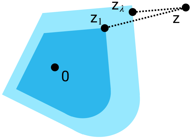
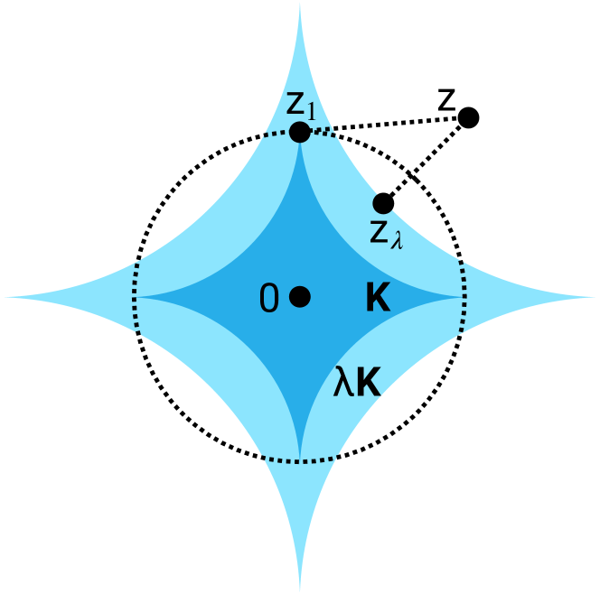
We introduce a result that to our knowledge is novel: the projection lemma. Given $z\in\mathbb{R}^{N}$, this lemma orders the one-parameter family of projections $z_{t}:=\mathrm{P}_{tK}(z)$ as a function of $t>0$ when $K$ is a closed and convex set with $0\in K$. Namely, as depicted in Figure 1(a), $\|\mathrm{P}_{tK}(z)\|_{2}\leq\|\mathrm{P}_{uK}(z)\|_{2}$ for $0<t\leq u<\infty$.

This lemma has immediate consequences for the ability of proximal algorithms to recover the $0$ vector from corrupted measurements. Note that the set $K$ need be neither symmetric nor origin-centered, but it must be convex, in general; we have included a pictorial counterexample in Figure 1(b) to depict why.

(a)

(b)

Figure 1: (1(a)) A visualization of the lemma. Projecting $z$ onto the outer and inner set gives $z_{\lambda}$ and $z_{1}$, respectively; evidently, $\|z_{1}\|_{2}\leq\|z_{\lambda}\|_{2}$. (1(b)) A counterexample using scaled $\ell_{p}$ balls for some $0<p<1$, suggesting why $K$ must be convex in general. Here, $z$ is projected inwards onto $\lambda K$, but towards a distal vertex when projected onto $K$.

Lemma 3.6 (Projection lemma).

Let $K\subseteq\mathbb{R}^{n}$ be a non-empty closed and convex set with $0\in K$, and fix $\lambda\geq 1$. For $z\in\mathbb{R}^{n}$,

$$\|\mathrm{P}_{K}(z)\|_{2}\leq\|\mathrm{P}_{\lambda K}(z)\|_{2}.$$

The following is an alternative version of Lemma 3.6 which quickly follows.

Corollary 3.7.

Let $K\subseteq\mathbb{R}^{n}$ be a non-empty closed and convex set with $0\in K$ and let $\|\cdot\|_{K}$ be the gauge of $K$. Given $y\in\mathbb{R}^{n}$ define

$$x_{\alpha}:=\operatorname*{\arg\min}\{\|x\|_{K}:\|x-y\|_{2}\leq\alpha\}$$

Then $\|x_{\alpha}\|_{2}$ is decreasing in $\alpha$.

Remark 3.8.

The proof of Lemma 3.6 examines the derivative of the function $f(t):=\|u_{t}\|_{2}^{2}$, where $u_{t}:=t\mathrm{P}_{\lambda K}(z)+(1-t)\mathrm{P}_{K}(z)$, and yields a growth rate of this derivative at $t=0$:

$$\frac{1}{2}\left.\frac{\mathrm{d}}{\mathrm{d}t}f(t)\right|_{t=0}=\langle z_{1},z_{\lambda}-z_{1}\rangle\geq\frac{\|z_{\lambda}-z_{1}\|_{2}^{2}}{\lambda-1}.$$

3.2 Tools from probability theory

For a full treatment of the topics herein, we refer the reader to [21, 42, 41, 1]. We start by defining subgaussian random variables and stating Hoeffding’s inequality, which characterizes how they concentrate in high dimensions.

Definition 3.9 ($\psi_{2}$-norm).

The subgaussian norm of a random variable $X$ is

$$\|X\|_{\psi_{2}}:=\sup_{p\geq 1}p^{-1/2}\big{(}\mathbb{E}|X|^{p}\big{)}^{1/p}$$

A random variable $X$ is subgaussian iff $\|X\|_{\psi_{2}}<\infty$.

Theorem 3.10 (General Hoeffding’s inequality [42, Theorem 2.6.3]).

Let $X_{i}$, $i=1,\ldots n$, be mean-zero subgaussian random variables and let $a\in\mathbb{R}^{n}$. For $t>0$,

$$\mathbb{P}\big{(}\big{|}\sum_{i=1}^{n}a_{i}X_{i}\big{|}\geq t\big{)}\leq e\cdot\exp\Big{(}\frac{-t^{2}}{C\sum_{i=1}^{n}a_{i}^{2}\|X_{i}\|_{\psi_{2}}^{2}}\Big{)}$$

One may define subexponential random variables in a way similar to subgaussian random variables. They, too, admit a concentration inequality.

Definition 3.11 ($\psi_{1}$ norm).

The subexponential norm of a random variable is

$$\|X\|_{\psi_{1}}:=\sup_{p\geq 1}p^{-1}\big{(}\mathbb{E}|X|^{p}\big{)}^{1/p}.$$

A random variable $X$ is subexponential iff $\|X\|_{\psi_{1}}<\infty$.

Theorem 3.12 (Bernstein’s inequality [42, Theorem 2.8.1]).

Let $X_{1},\ldots,X_{n}$ be independent mean-zero subexponential random variables. Then for all $\{a_{1},\ldots,a_{n}\}\in\mathbb{R}^{n}$,

$$\mathbb{P}\big{(}|\sum_{i=1}^{n}a_{i}X_{i}|\geq t\big{)}\leq 2\exp\Big{(}-C\min\Big{\{}\frac{t^{2}}{k^{2}\|a\|_{2}^{2}},\frac{t}{k\|a\|_{\infty}}\Big{\}}\Big{)},\qquad t\geq 0,k:=\max_{i}\|X_{i}\|_{\psi_{1}}$$

Finally, we introduce a result of Borell, Tsirelson, Ibragimov, and Sudakov about Gaussian processes, which states that the supremum of a Gaussian process defined over a topological space $T$ behaves nearly like a normal random variable. For a proof of this result, we refer the reader to [1].

Theorem 3.13 (Borell-TIS inequality [8, 39]).

Let $T$ be a topological space and let $\{f_{t}\}_{t\in T}$ be a centred (i.e., mean-zero) Gaussian process on $T$ with

$$\|f\|_{T} :=\sup_{t\in T}|f_{t}| \sigma_{T}^{2} :=\sup_{t\in T}\mathbb{E}\big{[}|f_{t}|^{2}\big{]}$$

such that $\|f\|_{T}$ is almost surely finite. Then $\mathbb{E}\|f\|_{T}$ and $\sigma_{T}$ are both finite and for each $u>0$,

$$\mathbb{P}\big{(}\|f\|_{T}>\mathbb{E}\|f\|_{T}+u\big{)}\leq\exp\big{(}-\frac{u^{2}}{2\sigma_{T}^{2}}\big{)}.$$

3.2.1 Refined bounds on Gaussian mean width

Two recent results yield improved upper- and lower-bounds on the GMW of convex polytopes intersected with Euclidean balls [5]. Each is integral to demonstrating $(\mathrm{BP}_{\sigma}^{*})$ parameter instability. The first describes how local effective dimension of a convex hull scales with neighbourhood size.

Proposition 3.14 ([5, Prop 1]).

Let $m\geq 1$ and $N\geq 2$. Let $T$ be the convex hull of $2N$ points in $\mathbb{R}^{m}$ and assume $T\subseteq B_{2}^{m}$. Then for $\gamma\in(0,1)$,

$$w(T\cap\gamma B_{2}^{m})\leq\min\big{\{}4\sqrt{\max\big{\{}1,\log(8eN\gamma^{2})\big{\}}},\gamma\sqrt{\min\{m,2N\}}\big{\}}$$

The second result shows that Proposition 3.14 is tight up to multiplicative constants.

Proposition 3.15 ([5, Prop 2]).

Let $m\geq 1$ and $N\geq 2$. Let $\gamma\in(0,1]$ and assume for simplicity that $s=1/\gamma^{2}$ is a positive integer such that $s\leq N/5$. Let $T$ be the convex hull of the $2N$ points $\{\pm M_{1},\ldots,\pm M_{N}\}\subseteq\mathbb{S}^{m-1}$. Assume that for some real number $\kappa\in(0,1)$ we have

$$\kappa\|\theta\|_{2}\leq\|M\theta\|_{2}\qquad\text{for all $\theta\in\mathbb{R}^{N}$ such that $\|\theta\|_{0}\leq 2s$},$$

Then

$$w(T\cap\gamma B_{2}^{m})\geq(\sqrt{2}/4)\kappa\sqrt{\log(N\gamma^{2}/5)}.$$

4 $(\mathrm{LS}_{\tau}^{*})$ parameter instability

We describe a parameter instability regime for $(\mathrm{LS}_{\tau}^{*})$, revealing a regime in which there is exactly one choice of parameter $\tau^{*}>0$ such that $\hat{R}(\tau^{*};x_{0},N,\eta)$ is minimax order-optimal. Specifically, Theorem 4.1 shows that $\hat{R}(\tau;x_{0},N,\eta)$ exhibits an asymptotic singularity in the limiting low-noise regime (by low-noise regime, we mean hereafter the regime in which $\eta\to 0$).

In 7.1 we complement this asymptotic result with numerical simulations that contrast how the three risks behave in a simplified experimental context. The numerics support that Theorem 4.1 provides accurate intuition to guide how $(\mathrm{LS}_{\tau}^{*})$ can be expected to perform in practice when the noise level is small relative to the magnitude of the signal’s entries.

The analogue of the classical CS result is included in our result as the special case $\tau=\tau^{*}=\|x_{0}\|_{1}$ (cf. Proposition 2.5). The cases for $\tau\neq\tau^{*}$ may seem surprising initially, but can be understood with the following key intuition: the approximation error is controlled by the effective dimension of the constraint set.

First, one should generally not expect good recovery when the signal lies outside the constraint set. When $\tau<\tau^{*}$, $y$ lies outside of the constraint set with high probability in the limiting low-noise regime. Accordingly, there is a positive distance between the true signal and the recovered signal which may be lower-bounded by a dimension-independent constant. Hence, the risk is determined by the reciprocal of the noise variance, growing unboundedly as $\eta\to 0$.

On the other hand, when $\tau>\tau^{*}$, $y$ lies within the constraint set with high probability in the limiting low-noise regime. Thus, the problem is essentially unconstrained in this setting, so the effective dimension of the constraint set for the problem should be considered equal to that of the ambient dimension. In particular, one should expect that the error be proportional to $N$.

Theorem 4.1 ($(\mathrm{LS}_{\tau}^{*})$ parameter instability).

Let $s\geq 1,\eta>0$ and let $x_{0}\in\Sigma_{s}^{N}\setminus\Sigma_{s-1}^{N}$. Given $\tau>0$,

$$\lim_{\eta\to 0}\hat{R}(\tau;x_{0},N,\eta)=\begin{cases}\infty&\tau<\|x_{0}\|_{1}\\ R^{*}(s,N)&\tau=\|x_{0}\|_{1}\\ N&\tau>\|x_{0}\|_{1}\end{cases}$$

In summary, the surprising part of this result is that there is a sharp phase transition between two unstable regimes, with the optimal regime lying on the boundary of the two phases. We argue this suggests that there is only one reasonable choice for $\tau$ in the low-noise regime. Observe, that Theorem 4.1 connects with Theorem 2.1 by taking the limit of the problem as $N\to\infty$ after first restricting to signals of a finite norm (arbitrarily, $1$) so that the essence of the result is preserved.

5 $(\mathrm{QP}_{\lambda}^{*})$ parameter instability

We show that $R^{\sharp}(\lambda;x_{0},N,\eta)$ is smooth in the low-noise regime. This result becomes evident from the closed-form expression for $R^{\sharp}(\lambda;s,N)$ that emerges for this special case. At first, this smoothness result seems to stand in contrast to the “cusp-like” behaviour that we observe analytically and numerically for $\lim_{\eta\to 0}\hat{R}(\tau;x_{0},N,\eta)$ (cf. Figure 3). However, $R^{\sharp}(\lambda;s,N)$ possesses unfavourable dependence on $N$ that is elucidated in Theorem 5.5.

Briefly, if the governing parameter $\lambda$ is too small, then the risk grows unboundedly as a power law of $N$ in high dimensions. This rate of growth implies that the risk is minimax suboptimal for such $\lambda$. To our knowledge, this result is novel. In contrast, for all suitably large $\lambda$, $R^{\sharp}(\lambda;s,N)$ admits the desirable property suggested in section 1: $R^{\sharp}(\lambda;s,N)\lesssim(\lambda/\lambda^{*})^{2}R^{*}(s,N)$. The result, stated in Theorem 5.8, essentially follows from known Lasso bounds for RIP matrices: $R(\lambda)\leq\lambda^{2}s$. Thus, in the low-noise regime, $R^{\sharp}(\lambda;x_{0},N,\eta)$ exhibits a phase transition between order-optimal and suboptimal regimes.

The numerics of section 7.2 suggest a viable constant for the growth rate of the risk when $\lambda$ is too small, and support Theorem 5.8 in the case where $\lambda$ is sufficiently large. These numerics also clarify the role that the dimension-dependent growth rate serves in the stability of $(\mathrm{QP}_{\lambda}^{*})$ about $\lambda^{*}$.

5.1 Smoothness of the risk

The $(\mathrm{QP}_{\lambda}^{*})$ estimator for a problem with noise level $\eta>0$ and with parameter $\lambda>0$ is given by soft-thresholding by $\eta\lambda$. In particular, $x^{\sharp}(\eta\lambda)$ is a smooth function with respect to the problem parameters, hence so is $R^{\sharp}(\lambda;x_{0},N,\eta)$ (being a composition of smooth functions). However, the closed form expression for $R^{\sharp}(\lambda;x_{0},N,\eta)$ is unavailable, because the expectations involved are untractable in general. When the noise-level vanishes this is no longer true and we may compute an exact expression in terms of $\lambda,s$ and $N$ for the risk. Specifically, we note that the smoothness result below is not special to the case where $\eta\to 0$, but is notable because of the closed form expression for the risk that is obtained.

Moreover, the result is notable, because the closed form expression is equivalent (in some precisely definable sense) to $R^{\sharp}(\lambda;x_{0},N,\eta)$ when $\eta>0$ and the magnitudes of the entries of $x_{0}$ are all large (i.e., “the signal is well-separated from the noise”). We make this connection after the main results discussed below. In turn, this connects Theorem 5.5 and Theorem 5.8 to Theorem 2.2, where the analytic expression is used to derive the so-called left-sided parameter instability and right-sided parameter stability results.

Proposition 5.1 ($R^{\sharp}(\lambda;x_{0},N,\eta)$ smoothness).

Let $s\geq 0,N\geq 1,x_{0}\in\Sigma_{s}^{N}$ and $\eta>0$. For $\lambda>0$,

$$\lim_{\eta\to 0}R^{\sharp}(\lambda;x_{0},N,\eta)=s(1+\lambda^{2})+2(N-s)\big{[}(1+\lambda^{2})\Phi(-\lambda)-\lambda\phi(\lambda)\big{]}$$ (2)

Remark 5.2.

Here and beyond, we denote the limiting low-noise risk by $R^{\sharp}(\lambda;s,N):=\lim_{\eta\to 0}R^{\sharp}(\lambda;x_{0},N,\eta)$; and define the function $G(\lambda):=(1+\lambda^{2})\Phi(-\lambda)-\lambda\phi(\lambda)$ for notational brevity, where $\phi$ and $\Phi$ denote the standard normal pdf and cdf, respectively.

An equivalence in behaviour is seen between the low-noise regime $\eta\to 0$ and the large-entry regime $|x_{0,j}|\to\infty$ for $j\in\mathrm{supp}(x_{0})$ with $\eta>0$. For both programs, the noise level is “effectively” zero by comparison to the size of the entries of $x_{0}$. This type of scale invariance allows us to re-state the previous result as a $\max$ formulation.

Corollary 5.3 ($\max$-formulation).

Let $s\geq 0,N\geq 1,x_{0}\in\Sigma_{s}^{N}$ and $\eta>0$. For $\lambda>0$,

$$\sup_{x_{0}\in\Sigma_{s}^{N}}R^{\sharp}(\lambda;x_{0},N,\eta)=R^{\sharp}(\lambda;s,N)$$

5.2 Left-sided parameter instability

We reveal an asymptotic regime in which $R^{\sharp}(\lambda;s,N)$ is minimax suboptimal for all $\lambda$ sufficiently small. The result follows from showing the risk derivative is large for all $\lambda<\bar{\lambda}$ when $s$ is sufficiently small relative to $N$. Here, $\bar{\lambda}:=\sqrt{2\log N}$ is an Ansatz estimate of $\lambda^{*}$ used to make the proof proceed cleanly. Finally, we show in what sense $\bar{\lambda}$ is asymptotically equivalent to $\lambda^{*}$ in Proposition 5.6.

The proof for the bound on the risk derivative follows by calculus and a standard estimate of $\Phi(-\lambda)$ in terms of $\phi(\lambda)$. Its scaling with respect to the ambient dimension destroys the optimal behaviour of $R^{\sharp}(\lambda;x_{0},N)$ for all $\lambda<\bar{\lambda}$. The proof of this result, stated in Theorem 5.5, follows immediately from Lemma 5.4 by the fundamental theorem of calculus.

Lemma 5.4 (risk derivative instability).

Fix $s\geq 1$. For any $\varepsilon\in(0,1)$, there exists $C>0$ and an integer $N_{0}=N_{0}(s)\geq s$ so that for all $N\geq N_{0}$

$$-\left.\frac{\mathrm{d}}{\mathrm{d}u}\right|_{u=1-\varepsilon}R^{\sharp}(u\bar{\lambda};s,N)\geq CN^{\varepsilon}$$

where $\bar{\lambda}=\sqrt{2\log(N)}$ is an estimate of the optimal parameter choice for $(\mathrm{QP}_{\lambda}^{*})$.

Theorem 5.5 ($(\mathrm{QP}_{\lambda}^{*})$ parameter instability).

Under the conditions of the previous lemma, for $\varepsilon\in(0,1)$ there exists a constant $C>0$ and integer $N_{0}\geq 1$ such that for all $N\geq N_{0}$,

$$R^{\sharp}((1-\varepsilon)\bar{\lambda};s,N)\geq C\frac{N^{\varepsilon}}{\log N}.$$

Though these results may initially seem surprising, we claim they are sensible when viewed in comparison to unregularized proximal denoising (i.e., $\lambda=0$). In this case, sparsity of the signal $x_{0}$ is unused and so one expects error be proporitional to the ambient dimension, as in section 4. In the low-noise regime, the sensitivity of the program to $\lambda$ is apparently amplified, and for $\lambda>0$ one may still expect $(\mathrm{QP}_{\lambda}^{*})$ to behave similarly to unregularized proximal denoising, begetting risk that behaves like a power law of $N$.

Proposition 5.6 (Asymptotic equivalence).

Let $N\in\mathbb{N}$ with $N\geq 2$, $s\in[N]$ and $\bar{\lambda}=\sqrt{2\log N}$. For given problem data, suppose $x^{\sharp}(\lambda)$ solves $(\mathrm{QP}_{\lambda}^{*})$, and let $\lambda^{*}$ be the optimal parameter choice for $R^{\sharp}(\lambda;s,N)$. Then

$$\lim_{N\to\infty}\frac{\bar{\lambda}}{\lambda^{*}}=1$$

Remark 5.7.

The value $\bar{\lambda}$ estimates the optimal parameter choice for $(\mathrm{QP}_{\lambda}^{*})$ in the following sense [30].

$$\lambda^{*}=O(\sqrt{\log(N/s)})\approx\sqrt{2\log N}=:\bar{\lambda}$$

5.3 Right-sided parameter stability

In the low-noise regime, $R^{\sharp}$ may still be order-optimal if $\lambda$ is chosen large enough. Specifically, if $\lambda=L\lambda^{*}$ for some $L>1$, then $R^{\sharp}(\lambda;x_{0},N)$ is still minimax order-optimal. We claim no novelty for the result of this section, but use it as a contrast to elucidate the previous theorem. Whereas for $\lambda<\bar{\lambda}$ we are penalized for under-regularizing in the low-noise regime in high dimensions, the theorem below implies that we are not penalized for over-regularizing.

Theorem 5.8.

$(\mathrm{QP}_{\lambda}^{*})$ is parameter stable in the sense that for any $\lambda>0$ satisfying $L=\lambda/\lambda^{*}>1$, there is $N_{0}=N_{0}(s,\lambda)\geq 2$ so that for all $N\geq N_{0}$,

$$\frac{R^{\sharp}(\lambda;s,N)}{R^{*}(s,N)}\leq CL^{2}.$$

Observe that the theorem still holds in the event that $\lambda^{*}$ is replaced by $\bar{\lambda}$. Thus, one may obtain the exact point of the phase transition, $\bar{\lambda}$, observed in Theorem 2.2. In fact, with this note, Theorem 2.2 follows as a direct consequence of the results of this section by letting $N\to\infty$.

6 $(\mathrm{BP}_{\sigma}^{*})$ parameter instability

The program $(\mathrm{BP}_{\sigma}^{*})$ is maximin suboptimal for very sparse vectors $x_{0}$. We show that $\tilde{R}(\sigma;x_{0},N,\eta)$ scales as a power law of $N$ for all $\sigma>0$. This rate is significantly worse than $R^{*}(s,N)$. When $x_{0}$ is very sparse and $(\mathrm{BP}_{\sigma}^{*})$ is underconstrained, then $\sigma\geq\eta N$ and 6.1 proves that $\tilde{R}(\sigma;x_{0},N,\eta)=\Omega(\sqrt{N})$. When $(\mathrm{BP}_{\sigma}^{*})$ is overconstrained, then $\sigma\leq\eta\sqrt{N}$ and 6.2, proves that $\tilde{R}(\sigma;x_{0},N,\eta)=\Omega(N^{q})$ for some $q>0$ when $x_{0}$ is very sparse.

Intuitively, $(\mathrm{BP}_{\sigma}^{*})$ kills not only the noise, but also eliminates too much of the signal content when underconstrained and $s$ is small compared to $N$. Because the signal is very sparse, destroying the signal content is disastrous to the risk. When overconstrained, the remaining noise overwhelms the risk, because the off-support has size approximately equal to the ambient dimension.

The above two steps are combined in Theorem 6.6 as a minimax formulation over all $\sigma>0$ and $x_{0}\in\Sigma_{s}^{N}$. In Theorem 6.10, this result is strengthened to a maximin statement over $x_{0}\in\Sigma_{s}^{N}$ and all $\sigma>0$.

Although these results may seem to run contrary to the apparent efficacy of the CS analogue of $(\mathrm{BP}_{\sigma}^{*})$ in empirical settings, we assure the reader that they are consistent. The type of parameter instability described in this section occurs at very large dimensions, in the setting where $s\geq 1$ is fixed. Thus, although these results bode poorly for the ability of $(\mathrm{BP}_{\sigma}^{*})$ to recover even the $0$ vector (arguably a desirable property of a denoising program), many structured high-dimensional signals observed in practice are not so sparse [in a basis] as to belong to the present regime. Nevertheless, this result serves as a caveat for the limits of a popular $\ell_{1}$ convex program.

6.1 Underconstrained $(\mathrm{BP}_{\sigma}^{*})$

The proof of this result uses standard methods from CS and may be found in 8.8.

Lemma 6.1.

Let $s\geq 1$ and let $x_{0}\in\Sigma_{s}^{N}\setminus\Sigma_{s-1}^{N}$ be an exactly $s$-sparse signal with $|x_{j}|\gtrsim N$ for all $j\in\mathrm{supp}(x_{0})$. If $\sigma>\eta\sqrt{N}$, then there exists a constant $C>0$ and integer $N_{0}=N_{0}(s)\geq 2$ such that if $N\geq N_{0}$ then

$$\tilde{R}(\sigma;x_{0},N,\eta)\geq C\sqrt{N}.$$

6.2 Overconstrained $(\mathrm{BP}_{\sigma}^{*})$

The proof that $\tilde{R}(\sigma;x_{0},N,\lambda)$ scales as a power law of $N$ when $\sigma\leq\eta\sqrt{N}$ proceeds by an involved argument, hinging on two major steps. The first step is to find an event whose probability is lower-bounded by a universal constant, on which $(\mathrm{BP}_{\sigma}^{*})$ fails to recover the $0$ vector when $\sigma=\eta\sqrt{N}$. Then, Lemma 3.6 extends this result to all $\sigma\leq\eta\sqrt{N}$. At this point, one may obtain the minimax result of Theorem 6.6, as well as a partial maximin result for all $x_{0}\in\Sigma_{s}^{N}$ on the restriction to $\sigma\leq\eta\sqrt{N}$. Then, to strengthen these claims to a maximin result over all $\sigma>0$, we prove a lemma that leverages elementary properties from convex analysis to show how the error of an estimator may be controlled by that of a lower dimensional estimator from the same class.

In this section, we state key results for building intuition and defer technical results and proofs to 8.8.

Theorem 6.2 (Overconstrained Maximin).

There exist universal constants $C>0,q\in(0,\frac{1}{2})$ and $N_{0}\geq 2$ an integer such that for all $N\geq N_{0},s\geq 0$ and $\eta>0$,

$$\sup_{x_{0}\in\Sigma_{s}^{N}}\inf_{\sigma\leq\eta\sqrt{N}}\tilde{R}(\sigma;x_{0},N,\eta)\geq CN^{q}.$$

By scaling, it is sufficient to prove this result in the case where $\eta=1$. The discussion below thus assumes $y=x_{0}+z$, while results are stated in full generality. The main result relies on proving

$$\inf_{\sigma\leq\sqrt{N}}\tilde{R}(\sigma;x_{0},N,1)\geq CN^{q}$$

when $x_{0}\equiv 0$, trivially implying the equation before it. Thus, the problem now becomes that of recovering the $0$ vector from standard normally distributed noise:

$$\tilde{x}(\sigma)=\operatorname*{\arg\min}\{\|x\|_{1}:\|x-z\|_{2}^{2}\leq\sigma^{2}\}.$$

Here and below, we denote the feasible set in $(\mathrm{BP}_{\sigma}^{*})$ by $F(z;\sigma)=B_{2}^{N}(z;\sigma)$ and use the notation $F:=F(z;\sqrt{N})$. For $\lambda>0$ and $0<\alpha_{2}\leq\alpha_{1}<\infty$, define $K_{i}=\lambda B_{1}^{N}\cap\alpha_{i}B_{2}^{N}$ to be the intersection of the $\ell_{1}$-ball scaled by $\lambda$ with the $\ell_{2}$-ball scaled by $\alpha_{i}$ for $i=1,2$.

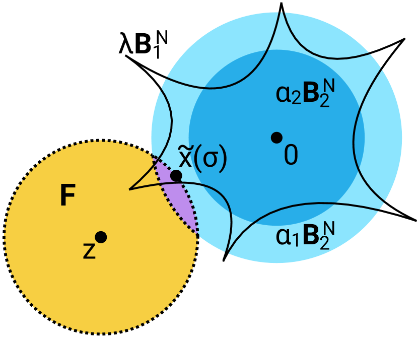
With $\sigma=\sqrt{N}$, we prove a geometric lemma. A pictorial representation of this lemma appears in Figure 2, in which we have represented $\lambda B_{1}^{N}$ using Milman’s 2D representation of high-dimensional $\ell_{1}$ balls to facilitate the intuition for how they behave in the present context. The key to the proof of Theorem 6.2 is the geometric lemma below, Lemma 6.3. It proves there exists an $\ell_{1}$ ball of radius $\lambda$ that intersects the feasible set, hence a solution $\tilde{x}(\sigma)$ must satisfy $\|\tilde{x}(\sigma)\|_{1}\leq\lambda$. Further, it shows that any vector in the ball $\lambda B_{1}^{N}$ which has small Euclidean norm does not intersect the feasible set. Thus, the solution must have large Euclidean norm.

Finally, this geometric lemma verifies that the previous three conditions occur on an event occurring with at least probability $k_{3}>0$. As an immediate consequence, this lemma yields a lower risk bound, Corollary 6.4. The integers $N_{0}^{\eqref{prop:bppd-oc-1b}},N_{0}^{\eqref{prop:bppd-oc-2b}}$ are defined in the technical results of 8.8.2.

Lemma 6.3 (Geometric lemma).

Let $K_{1},K_{2},F$ be defined as above. Let $N_{0}^{\eqref{lem:bppd-oc-3a}}:=\max\{N_{0}^{\eqref{prop:bppd-oc-1b}},N_{0}^{\eqref{prop:bppd-oc-2b}}\}$ be a universal constant and suppose $N>N_{0}^{\eqref{lem:bppd-oc-3a}}$. There are universal constants $k_{3}=k_{3}(N_{0}^{\eqref{lem:bppd-oc-3a}})>0$, $C_{3},q>0$, and an event $\mathcal{E}$ such that

1. $K_{1}\cap F\neq\emptyset$

1. $K_{2}\cap F=\emptyset$

1. $\alpha_{2}>C_{3}N^{q}$

1. $\mathbb{P}(\mathcal{E})>k_{3}$.

Figure 2: A visualization of the lemma. We use Milman’s 2D representation of high-dimensional $\ell_{1}$ balls to facilitate the intuition. In this setting, $\tilde{x}(\sigma)$ must lie inside $\lambda B_{1}^{N}$. On the event $\mathcal{E}$ described by the lemma, one simultaneously finds $K_{1}\cap F\neq\emptyset$ and $K_{2}\cap F=\emptyset$.

Corollary 6.4.

Fix $\eta>0$. There are universal constants $C,q>0$ such that for all $N\geq N_{0}^{\eqref{lem:bppd-oc-3a}}$,

$$\tilde{R}(\eta\sqrt{N};0,N,\eta)\geq CN^{q}.$$

Next we extend Corollary 6.4 from the case where $\sigma=\sqrt{N}$ to any positive $\sigma\leq\sqrt{N}$. The proof of this result follows near immediately from the projection lemma in Lemma 3.6. Thus, one finds $\tilde{x}(\sigma)$ has Euclidean norm at least as large as $\tilde{x}(\sqrt{N})$ when $\tilde{x}(\sigma)$ is an estimator of the $0$ vector.

Lemma 6.5.

Let $0<\sigma_{1}<\sigma_{0}=\sqrt{N}$ and $x_{0}\equiv 0$. Define $\tilde{x}(\sigma_{0}),\tilde{x}(\sigma_{1})$ as in $(\mathrm{BP}_{\sigma}^{*})$ for $\sigma=\sigma_{0},\sigma_{1}$, respectively. Then $\|\tilde{x}(\sigma_{1})\|_{2}^{2}\geq\|\tilde{x}(\sigma_{0})\|_{2}^{2}$. Moreover, for $N\geq 2$,

$$\mathbb{E}\|\tilde{x}(\sigma_{1})\|_{2}^{2}\geq\mathbb{E}\|\tilde{x}(\sigma_{0})\|_{2}^{2}.$$

6.3 Minimax results

We now have the tools to state a minimax instability result for $(\mathrm{BP}_{\sigma}^{*})$. Informally, the best worst-case risk scales as a power law of $N$ in the very sparse regime. In particular, for $s$ fixed and $N$ sufficiently large, there is no choice of $\sigma>0$ yielding order-optimal risk for its corresponding worst-case signal.

Theorem 6.6 (Minimax Suboptimality).

There are universal constants $C>0,q\in(0,\frac{1}{2}],N_{0}\geq 2$ such that for all $N\geq N_{0},\eta\geq 0$ and $s\geq 1$,

$$\adjustlimits{\inf}_{\sigma>0}{\sup}_{x\in\Sigma_{s}^{N}}\tilde{R}(\sigma;x,N,\eta)\geq CN^{q}$$

6.4 Maximin results

The final result of this section establishes maximin parameter instability for all $x_{0}\in\Sigma_{s}^{N}$ and $\sigma>0$. To do this, we must show there exists a choice of signal $x_{0}\in\mathbb{R}^{N}$ admitting no choice of $\sigma>0$ bestowing order optimal recovery error. To this end, we will demonstrate that the previous overconstrained instability results extend to $s$-sparse signals with $s\geq 1$. This will be enough to yield a choice of $x_{0}$ whose recovery is suboptimal over the whole parameter range.

Lemma 6.7 (Overconstrained $(\mathrm{BP}_{\sigma}^{*})$, $s\geq 1$).

Let $x_{0}\in\Sigma_{s}^{N}$ with $\mathrm{supp}(x_{0})\subseteq T\subseteq[N]$, let $y=x_{0}+\xi$ for some $\xi\in\mathbb{R}^{N}$, let $x_{1}:=(x_{0})_{T^{C}}\in\Sigma_{0}^{N-s}$ and fix $\sigma>0$. Let $\tilde{x}=\tilde{x}(\sigma)\in\mathbb{R}^{N}$ be the solution of $(\mathrm{BP}_{\sigma}^{*})$ where $x_{0}$ is the ground truth, and let $\tilde{x}^{\prime}=\tilde{x}^{\prime}(\sigma)\in\mathbb{R}^{N-s}$ be the solution of $(\mathrm{BP}_{\sigma}^{*})$ where $x_{1}$ is the ground truth. Then

$$\|\tilde{x}_{T^{C}}\|_{2}\geq\|\tilde{x}^{\prime}\|_{2}.$$

An immediate consequence of this result is the following inequality between the Euclidean norms of the error vectors.

Corollary 6.8.

Let $h:=\tilde{x}-x_{0}$ and $h^{\prime}:=\tilde{x}^{\prime}-x_{1}$, where $x_{0},x_{1},\tilde{x},\tilde{x}^{\prime}$ are defined as above. Then,

$$\|h\|_{2}\geq\|h^{\prime}\|_{2}.$$

Remark 6.9.

The above corollary is not yet sufficient to imply the desired maximin result below. As per the lemma, if $N-s\geq N_{0}^{\eqref{lem:bppd-oc-3a}}$ then $\tilde{x}^{\prime}$ is parameter unstable for $\sigma\leq\sqrt{N-s}$ and so $\tilde{x}$ is, too. The fix for this slight mismatch is trivial, but technical. The result can be extended to the range $\sigma\leq\sqrt{N}$ by adjusting the constants in the proof of Lemma 6.3 and its constituents, leveraging the fact that $(N-s)/N\to 1$ as $N\to\infty$ and re-selecting $N_{0}^{\eqref{lem:bppd-oc-3a}}$ if necessary. We omit the details of this technical exercise.

We proceed under the assumption that the constants have been tuned to allow for $\tilde{x}^{\prime}$ parameter instability to imply $\tilde{x}$ parameter instability for all $\sigma\leq\sqrt{N}$. Thus equipped, we state the following maximin parameter instability result for $(\mathrm{BP}_{\sigma}^{*})$. The proof of this result proceeds by finding a signal $x_{0}\in\Sigma_{s}^{N}$ such that $\tilde{R}(\sigma;x_{0},N,\eta)$ is suboptimal for all $\sigma>0$. Since Lemma 6.1 applies only to signals $x_{0}$ with at least one non-zero entry, one shows there exists such a signal which simultaneously admits poor risk for $\sigma\leq\eta\sqrt{N}$ and $\sigma\geq\eta\sqrt{N}$. For example, it is enough to take $x_{0}:=Ne_{1}$ where $e_{1}\in\mathbb{R}^{N}$ is the first standard basis vector.

Theorem 6.10 ($(\mathrm{BP}_{\sigma}^{*})$ maximin suboptimality).

There are universal constants $C>0,q\in(0,\frac{1}{2}]$ and $N_{0}\geq 1$ such that for all $N\geq N_{0}$

$$\sup_{x_{0}\in\Sigma_{s}^{N}}\inf_{\sigma>0}\tilde{R}(\sigma;x_{0},N,\eta)\geq CN^{q}.$$

Remark 6.11.

The current result is given in a maximin framework. This framework is stronger than the minimax one in which these types of results are typically framed. In essence, the maximin framework assumes that the minimizer has knowledge about the ground truth signal $x_{0}$; even still it is not possible to choose $\sigma$ to achieve order-optimal risk.

7 Numerical Results

Let $\mathfrak{P}\in\{\text{{$(\mathrm{LS}_{\tau}^{*})$}, {$(\mathrm{QP}_{\lambda}^{*})$}, {$(\mathrm{BP}_{\sigma}^{*})$}}\}$ be a PD program with solution $x^{*}(\varrho)$ where $\varrho\in\{\tau,\lambda,\sigma\}$ is the associated parameter. Given a signal $x_{0}$ and noise $\eta z$, denote by $\mathcal{L}(\varrho;x_{0},N,\eta z)$ the loss associated to $\mathfrak{P}$ and define $\varrho^{*}=\varrho(x_{0},\eta)>0$ to be the value of $\varrho$ yielding best risk (i.e., where $\mathbb{E}_{z}\mathcal{L}(\varrho;x_{0},N,\eta z)$ is minimal). We say the normalized parameter $\rho$ for the problem $\mathfrak{P}$ is given by $\rho:=\varrho/\varrho^{*}$ and note that $\rho=1$ is a population estimate of the argmin of $\mathcal{L}(\varrho;x_{0},N,\eta\hat{z})$; by the law of large numbers, this risk estimates well an average of such losses over many realizations $\hat{z}$. Finally, define the auxiliary function $L(\rho;x_{0},N,\eta\hat{z}):=\mathcal{L}(\rho\varrho^{*};x_{0},N,\eta\hat{z})$.

The plots in Figures Figure 3(a), Figure 3(b), Figure 4(b), Figure 5(a) and Figure 6 visualize the average loss,

$$\bar{L}(\rho_{i};x_{0},N,\eta,k):=\frac{1}{k}\sum_{j=1}^{k}L(\rho_{i};x_{0},N,\eta\hat{z}_{ij})$$ (3)

for each program, evaluated on a grid $\{\rho_{i}\}_{i=1}^{n}$ of size $n$ and plotted on a $\log$-$\log$ scale, where $L(\rho;x_{0},N,\eta\hat{z})=\eta^{-2}\|x^{*}(\varrho)-x_{0}\|_{2}^{2}$. Here, each of the $nk$ realizations of the noise is distributed according to $\hat{z}_{ij}\sim\mathcal{N}(0,1)$, the noise level given by $\eta$ and the signal by $x_{0}$ where $x_{0}=N\sum_{i=1}^{s}e_{i}$ with $e_{i}$ being the $i$th standard basis vector. The grid $\{\rho_{i}\}_{i=1}^{n}$ was logarithmically spaced and centered about $\rho_{(n+1)/2}=1$ with $n$ always odd. The solutions to each PD problem were obtained using standard available methods in Python: sklearn’s minimize_scalar function from the optimize module was used for solving $(\mathrm{LS}_{\tau}^{*})$ and $(\mathrm{BP}_{\sigma}^{*})$ [33], while the solution to $(\mathrm{QP}_{\lambda}^{*})$ was obtained via soft-thresholding. Finally, the optimal values $\tau^{*},\lambda^{*}$ and $\sigma^{*}$ were either determined analytically (e.g., $\tau^{*}=\|x_{0}\|_{1}$), or estimated on a dense grid about an approximately optimal value for that parameter. Initial guesses for $\sigma^{*}$ and $\lambda^{*}$ were $\eta\sqrt{N}$ and $\sqrt{2\log(N/s)}$ respectively.

7.1 $(\mathrm{LS}_{\tau}^{*})$ numerical simulations

(a)

(b)

Figure 3: $(\mathrm{LS}_{\tau}^{*})$ parameter instability in the low-noise regime. Average loss as per (3) for each program plotted on a $\log$-$\log$ scale with respect to the normalized parameter. The data parameters for (a) are $(s,N,\eta,k,n)=(20,10^{3},10^{-3},150,301)$ and those for (b) are $(s,N,\eta,k,n)=(20,10^{6},10^{-3},50,301)$.

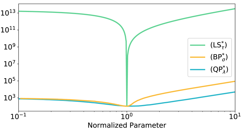
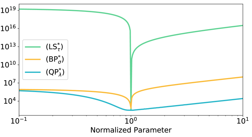
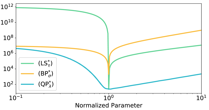
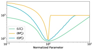
This section presents numerical simulations demonstrating parameter instability of $(\mathrm{LS}_{\tau}^{*})$ in the low-noise regime for two different ambient dimensions $N=10^{3},10^{6}$. This repetition has the benefit of showcasing the behaviour of $(\mathrm{LS}_{\tau}^{*})$ at two different sparsity levels, as well as contrasting the behaviour of $(\mathrm{LS}_{\tau}^{*})$ with $(\mathrm{QP}_{\lambda}^{*})$ and $(\mathrm{BP}_{\sigma}^{*})$ at relatively low and high dimensions. Using the notation above, $n=301$ points and $s=20$; $(k,N)=(150,10^{3})$ for Figure 3(a), while $(k,N)=(50,10^{6})$ for Figure 3(b). In both regimes, $x_{0}$ is quite sparse $s/N\sim 10^{-2},10^{-5}$ with entries that are well separated from the noise $N/\eta\sim 10^{6},10^{9}$.

We may glean several pieces of information from these two plots. Most notably, the $(\mathrm{LS}_{\tau}^{*})$ parameter instability manifests in very low dimensions, relative to practical problem sizes. Moreover, the curve for $(\mathrm{LS}_{\tau}^{*})$ average loss seems to approach something resembling the sharp asymptotic phase transition described by Theorem 4.1. One may also notice the behaviour of the other two programs in the low-noise regime. It is apparent that the magnitude of the derivative for the $(\mathrm{QP}_{\lambda}^{*})$ risk increases markedly on the left-hand side of the optimal normalized parameter value (i.e., below $1$) between the $N=10^{3}$ and $N=10^{6}$ plots. This behaviour is consistent with the result in Theorem 5.5 that the left-sided risk scales as a power law of $N$.

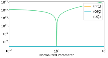
Finally, we observe that $(\mathrm{BP}_{\sigma}^{*})$ develops a shape resembling the instability of $(\mathrm{LS}_{\tau}^{*})$ when $N=10^{6}$. We offer the plausible explanation that the relative sparsity of the signal is small ($s/N=2/10^{5}$) and thus this regime coincides with the regime in which $(\mathrm{BP}_{\sigma}^{*})$ develops parameter instability. Figure 5 demonstrates that such an instability seems to occur in very large dimensions, a suspicion corroborated by the remark at the end of 7.3.

We observe that the parameter instability developed by $(\mathrm{BP}_{\sigma}^{*})$ seems to manifest in a way similar to that of $(\mathrm{LS}_{\tau}^{*})$. This is interesting, because Theorem 6.10 shows that there is no good choice of parameter $\sigma$, though Figure 5 supports that there is a single best choice, albeit minimax suboptimal, when $N$ is moderately large.

7.2 $(\mathrm{QP}_{\lambda}^{*})$ analytic plots

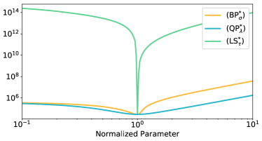
We plot $R^{\sharp}(\lambda;s,N)$ using the expressions derived in (2). Observe that the plot of the analytic expression for $R^{\sharp}(\lambda;s,N)$ agrees well with the simulations of $R^{\sharp}(\lambda;x_{0},N,\eta)$ in Figure 3 and Figure 5.

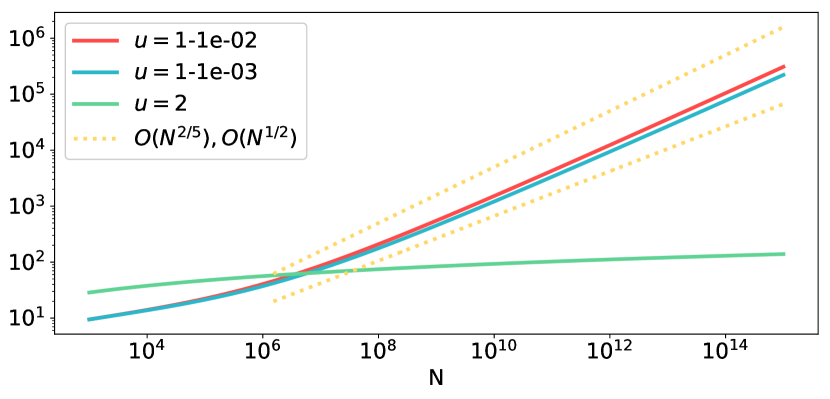
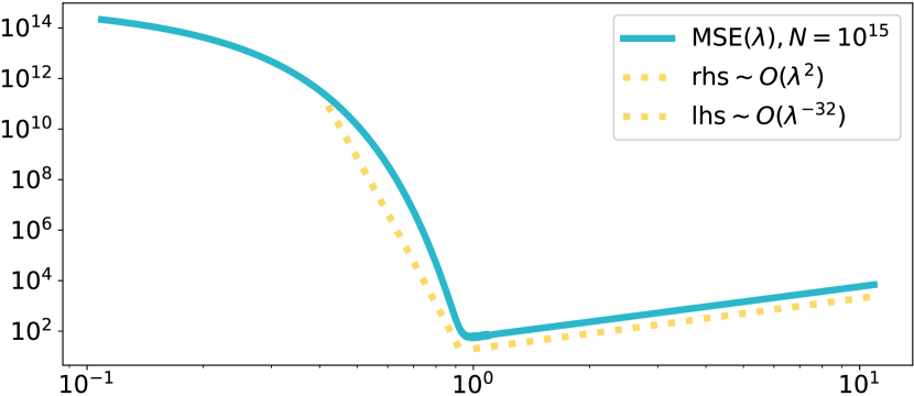
In Figure 4(a) we plot $R^{\sharp}(\lambda;s,N)$ for $\lambda\in\{1-10^{-2},1-10^{-3},2\}$. It is evident from the reference lines $y\sim N^{2/5}$ and $y\sim\sqrt{N}$ that $R^{\sharp}(u\bar{\lambda};s,N)$ scales like a power law of $N$ for $u<1$, while $R^{\sharp}(2\bar{\lambda};s,N)$ appears to have approximately order-optimal growth. The derivatives of these three functions are visualized in Figure 4(c), with plotted reference lines $y=N^{2/5},\sqrt{N}$. Again, it is evident that the derivative scales as a power law of $N$ for those risks with $\lambda<\bar{\lambda}$. In Figure 4(b) we plot $R^{\sharp}(\lambda;s,N)$ as a function of $\lambda$ for $N=10^{15}$. One may observe parameter instability for $\lambda<\lambda^{*}$, for example by comparison to the plotted reference line $y\sim\lambda^{-32}$. Similarly, one may observe right-sided parameter stability of $R^{\sharp}(\lambda;s,N)$ by comparing with the second plotted reference line, $y\sim\lambda^{2}$. From these simulations one may observe that choosing $\lambda=.5\lambda^{*}$ accrues at least a $10^{9}$ fold magnification of the error.

Finally, we would like to clarify a potentially confusing issue. Though our theory for $(\mathrm{QP}_{\lambda}^{*})$ refers to $\lambda^{*}$ only through its connection with $\bar{\lambda}$, we were able to approximate $\lambda^{*}$ empirically in our numerical simulations. Accordingly, we have made reference to it when discussing parameter stability regimes.

(a)

(b)

(c)

Figure 4: $(\mathrm{QP}_{\lambda}^{*})$ parameter instability in the low-noise regime. All curves are generated analytically using the expressions obtained in section 5 and plotted on a $\log$-$\log$ scale. (a) A plot of $R^{\sharp}(u\lambda^{*};s,10^{15})$ as a function of $N$ for $u\in\{1-10^{-2},1-10^{-3},2\}$. The lines $y=N^{2/5}/15$, $y=\sqrt{N}/20$ are plotted for reference. (b) A plot of $R^{\sharp}(\lambda;s,10^{15})$ as a function of $\lambda$. Two lines are plotted as reference for risk growth rate with respect to $\lambda$. (c) A plot of the magnitude of $\frac{\mathrm{d}}{\mathrm{d}u}R^{\sharp}(u\lambda^{*};s,10^{15})$ as a function of $N$ for $u\in\{1-10^{-2},1-10^{-3},2\}$. The lines $y=N^{2/5}$, $y=\sqrt{N}/20$ are plotted as reference.

7.3 $(\mathrm{BP}_{\sigma}^{*})$ numerical simulations

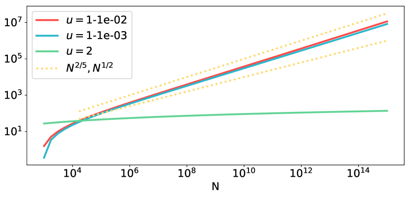
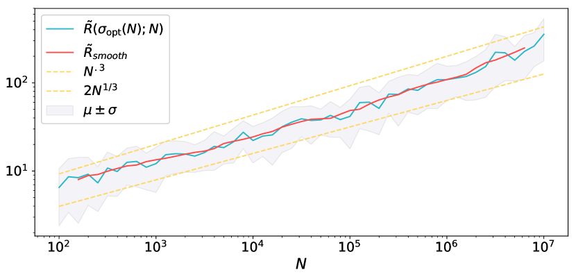
This section presents numerical simulations demonstrating parameter instability of $(\mathrm{BP}_{\sigma}^{*})$ in the regime where $x_{0}$ is very sparse. Figure 5(a) is generated as described by the above procedure in section 7, with parameters $(N,s,\eta,k,n)=(10^{7},1,1,10,237)$, while Figure 5(b) was generated in a way that mirrors the proof of Theorem 6.10, with parameters $(s,\eta,k,n)=(1,1,25,31)$.

The thrust of Figure 5(a) is to resolve parameter instability of $(\mathrm{BP}_{\sigma}^{*})$ about the optimal parameter choice. Because the theory suggests that $\tilde{R}(\sigma;x_{0},N,\eta)$ is surely resolved when the ambient dimension is sufficiently large, we set $N=10^{7}$; this value was expected to resolve the instability, as per the discussion in 7.3.1 below. We limited the number of realizations and grid points because the problem size was computationally prohibitive. The minimal average loss observed on the plot was significantly larger than the respective minimal average losses of $(\mathrm{LS}_{\tau}^{*})$ and $(\mathrm{QP}_{\lambda}^{*})$ by a factor of $82.2$, supporting the theory. We also noticed a cusp-like behaviour, which would be an interesting object of further study.

Figure 5(b) was generated so as to mirror the theory backing Theorem 6.10. Specifically, noise realizations were constrained to the constant probability event $\{\|z\|_{2}^{2}-N\in(.5\sqrt{N},5\sqrt{N})\}$. Plotted in the figure is the average best loss as a function $N$,

$$\bar{L}_{\text{best}}(N;x_{0},\eta,k,n):=\frac{1}{k}\sum_{j=1}^{k}\min_{i\in[n]}L(\sigma_{i}(N);x_{0},N,\eta\hat{z}_{ij}).$$

The domain for $N$ ranges from $10^{2}$ to $10^{7}$, computed on a logarithmically spaced grid composed of $51$ points. For each value $N$ in the grid, the average loss was computed for $n=31$ values of $\sigma$, each using $k=25$ realizations $\hat{z}$ of the noise. The standard deviations of the best loss realizations were computed, and plotted as a grey ribbon about the average best loss. Included for reference is a smoothed version of the average best loss, computed as a rolling window average. In addition, we have plotted two power laws of $N$ that lower- and upper-bound the averaged best loss, and nearly bound that quantity up to a full standard deviation.

(a)

(b)

Figure 5: $(\mathrm{BP}_{\sigma}^{*})$ parameter instability in the very sparse regime. (a) Data parameters: $(s,N,\eta,k,n)=(1,10^{7},1,10,237)$. Average losses plotted on a $\log$-$\log$ scale with respect to the normalized parameter. (b) Average best loss for $(\mathrm{BP}_{\sigma}^{*})$ as a function of $N$. Data parameters: $(s,\eta,k,n)=(1,1,25,31)$. The function $\sigma_{\text{opt}}(N)$ was obtained as the value of $\sigma$ bestowing minimal loss of the program for each $N$ and realization. These best losses were averaged, yielding average best loss. The standard deviation was computed for each $N$ from the same loss realizations and included as a ribbon about the mean; functions $y=N^{3/10}$ and $y=2N^{1/3}$ are included for reference.

7.3.1 Simulating theorem parameters

Here we clarify the relationship between some of the constants appearing in the proofs of Theorem 6.6 and Theorem 6.10. We provide two examples of minimal $N_{0}$ values guaranteeing parameter instability behaviour of $(\mathrm{BP}_{\sigma}^{*})$ for given parameter choices. The theory does not claim these values to be optimal, nor do we claim that the constants are tuned. In particular, these demonstrations seem rather pessimistic, especially by comparison with the numerical simulations in Figure 5.

The following values were determined by computing $N_{0}:=\max\{N_{0}^{\eqref{prop:bppd-oc-1a}}(a_{1},C_{1},L),N_{0}^{\eqref{prop:bppd-oc-2a}}(C_{2},L)\}$ for particular choices of $a_{1},C_{1},C_{2}$ and $L$, using their definitions in the technical results of 8.8.2. Thus, the theory of section 6 guarantees parameter instability for all $N\geq N_{0}$ when

$$N_{0}\approx 1.5\rm{e}6 \quad\text{and}\quad(a_{1},C_{1},C_{2},L)\approx(1.45,5,4,3.78)\qquad\text{or}$$

$$N_{0}\approx 4.9\rm{e}5 \quad\text{and}\quad(a_{1},C_{1},C_{2},L)\approx(1.58,4.04,4,3.62).$$

These numbers appear pessimistic, given that $N_{0}$ is large, while $(C_{2},C_{1})\approx(4,5)$ implies the instability arises on the event $\{\|z\|_{2}^{2}-N\in(4\sqrt{N},5\sqrt{N})\}$, which occurs with relatively minute (but constant) probability. Thus, it may not be all that surprising that $(\mathrm{BP}_{\sigma}^{*})$ suboptimality is difficult to ascertain empirically from a small number of realizations in only moderately large dimension when $\sigma\approx\sigma^{*}$.

7.4 Parameter stability in sparse proximal denoising

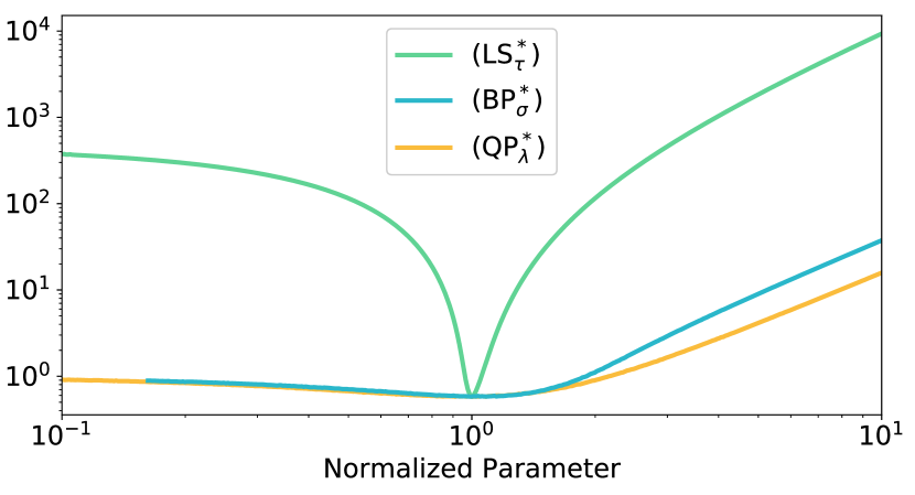
In this section we show numerical simulations in which the three programs appear to exhibit better parameter stability. For these simulations, $\eta\approx 233.0$, $s=2500$ and $N=10^{4}$. Average loss was computed from $k=25$ realizations for $n=401$ grid points. As the noise is large, this setting lies (mostly) outside the regime in which $(\mathrm{LS}_{\tau}^{*})$ and $(\mathrm{QP}_{\lambda}^{*})$ exhibit parameter instability. Moreover, the signal is not very sparse, since $s/N=.25$. Thus, this setting also lies outside the regime in which $(\mathrm{BP}_{\sigma}^{*})$ exhibits parameter instability. Accordingly, smooth risk curves are seen for $(\mathrm{BP}_{\sigma}^{*})$ and $(\mathrm{QP}_{\lambda}^{*})$. While $(\mathrm{QP}_{\lambda}^{*})$ and $(\mathrm{BP}_{\sigma}^{*})$ appear relatively gradual, $(\mathrm{LS}_{\tau}^{*})$ appears at least to avoid a cusp-like point about $\tau/\tau^{*}=1$. These data visualized in Figure 6.

Figure 6: Parameter stability of sparse PD programs when $(s,N,\eta,k,n)=(2500,10^{4},233,25,401)$. Plotted curves represent average loss, plotted on a $\log$-$\log$ scale.

7.5 Realistic denoising examples

7.5.1 Image-space denoising

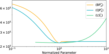
We visualize how proximal denoising behaves for a realistic denoising problem. The ground truth signal is the standard $512\times 512\times 3$ colour image of a mandrill face, ravelled to a vector $x_{0}\in[0,1]^{N}\subseteq\mathbb{R}^{N}$, $N=786\,432$. The denoising is performed in image space. Specifically, the signal $x_{0}$ is not sparse: $99.98\%$ of its coefficients are nonzero. We set $y_{j}=x_{0,j}+\eta z_{j}\in\mathbb{R}^{N}$ where $\eta=10^{-5},1$ and $z_{j}\overset{\text{iid}}{\sim}\mathcal{N}(0,1)$. The results of this example are displayed in Figure 7: the ground truth and noisy images in the top row, and quantitative results captured by plots of the average loss (3) in the bottom row.

The plots of average loss were generated from $k=25$ realizations of noise $z$, with a logarithmically spaced grid of $n=501$ points centered about the optimal parameter value for each of the three proximal denoising programs. The optimal parameter value for each program was determined analytically where possible, or numerically using standard solvers [25]. A smooth approximating curve of the non-uniformly spaced point cloud of loss realizations was computed using radial basis function approximation. The RBF approximation used multiquadric kernels with parameters $(\varepsilon_{\text{rbf}},\mu_{\text{rbf}},n_{\text{rbf}})=(10^{-3},10^{-2},301)$. Here, $\varepsilon_{\text{rbf}}$ is the associated RBF scale parameter, $\mu_{\text{rbf}}$ is a smoothing parameter and $n_{\text{rbf}}$ is the number of grid points at which to approximate [25]. The RBF parameters for the approximation were selected so as to generate a smooth line that best represents the path about which the individual (noisy) data points concentrate.

About the optimal average loss (where the normalized parameter is $1$), an average difference of $1.382\%$ in the value of $\tau$ results in a $4.694\times 10^{5}$ fold difference in nnse on average when $\eta=10^{-5}$. In contrast, that error varies by no more than a factor of three in the large noise regime ($\eta=1$). Moreover, we observe that the average losses computed for $\eta=10^{-5}$ upper bound those computed for $\eta=1$. These results suggest not to use $(\mathrm{LS}_{\tau}^{*})$ for proximal denoising when $\eta$ is small, even when the underlying data are not sparse.

Figure 7: Top (left-to-right): The underlying signal is the $512\times 512\times 3$ mandrill image; the middle image is corrupted by iid normally distributed noise ($\eta=10^{-5}$); the right-most image is corrupted by iid normally distributed noise ($\eta=1$). The pixel values of the original image lie in $[0,1]^{3}$; those of the noisy images are scaled to this range for plotting. Bottom: Average loss is plotted with respect to the normalized parameter for $(\mathrm{LS}_{\tau}^{*})$, $(\mathrm{QP}_{\lambda}^{*})$ and $(\mathrm{BP}_{\sigma}^{*})$ respectively when $\eta=10^{-5}$ (left) and $\eta=1$ (right). The associated parameters are $(N,k,n)=(786\,432,25,501)$. Plotted lines are smoothed approximations of loss realization data using multiquadric RBFs.

7.5.2 1D denoising example

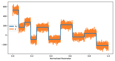
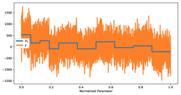
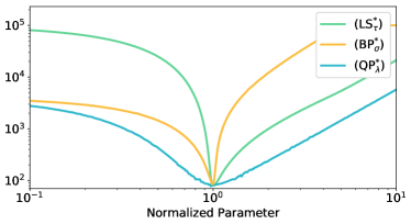
In this section, we demonstrate parameter instability regimes for a realistic example of a 1D signal using wavelet domain denoising. Specifically, an $s$-sparse 1D signal $x_{0}\in\mathbb{R}^{N}$ was generated in the Haar wavelet domain, where $(s,N)=(10,4096)$. In the signal domain, iid normal random noise was added to the signal to generate $\mathcal{W}^{-1}y:=\mathcal{W}^{1}x_{0}+\eta z$ where $\eta=\frac{N}{100},\frac{N}{10}$. The denoising problem was solved in the wavelet domain on a grid of size $501$ centered about the optimal normalized parameter and logarithmically spaced. Namely, the input to each program was $y$. The loss was computed in the signal domain after applying the inverse transform to the estimated solution:

$$L(\rho;x_{0},N,\eta\hat{z}):=\eta^{-2}\|\mathcal{W}^{-1}(x^{*}(\rho)-x_{0})\|_{2}^{2}$$

A smooth approximation to the average loss $\bar{L}(\rho_{i};x_{0},N,\eta,k)$ was computed from $k=25$ realizations of the noise using linear radial basis function approximation with parameters $(\mu_{\text{rbf}},n_{\text{rbf}})=(0.01,501)$.

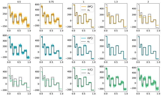
In Figure 8, we visualize how the three programs behave for denoising a 1D signal, sparse in the Haar wavelet domain, which has been corrupted by one of two different noise levels in the signal domain. The top row visualizes the ground truth signal with a realization of the corrupted signal for $\eta=N/100$ (top-left) and $\eta=N/10$ (top-right). The bottom row visualizes the average loss with respect to the normalized parameter of each program. In the high-noise regime (bottom-right), it is clearly seen that $(\mathrm{BP}_{\sigma}^{*})$ is the most parameter unstable about the optimal parameter choice. Moreover, the best average loss for $(\mathrm{BP}_{\sigma}^{*})$ is greater than that for $(\mathrm{QP}_{\lambda}^{*})$ or $(\mathrm{LS}_{\tau}^{*})$, as suggested by the supporting theory. We note that $(\mathrm{QP}_{\lambda}^{*})$ also has an average loss greater than the minimal one, and suggest — noting the local variability in the curve — that this is an artifact of the RBF approximation through the optimality region. In the moderate-noise regime, we see a situation in which $(\mathrm{QP}_{\lambda}^{*})$ appears to be the most parameter stable — again consistent with our reasoning that unconstrained programs should exhibit better stability. In contrast, $(\mathrm{LS}_{\tau}^{*})$ is most parameter unstable below the optimal parameter, while it is $(\mathrm{BP}_{\sigma}^{*})$ that is most parameter unstable above the optimal parameter. This behaviour may be indicative of a regime intermediate to those we have previously discussed (i.e., lying between strictly low-noise and strictly very sparse).

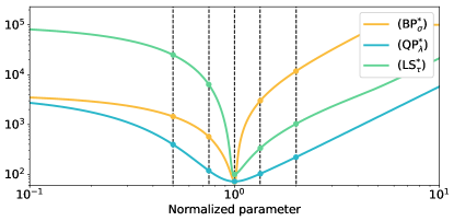
With the grid in Figure 9, we intend to elucidate how parameter instability manifests for each program as a function of the normalized parameter, by visualizing the recovered signal for different values of the normalized parameter. The top plot shows the same average losses that are plotted in the bottom-left of Figure 8. The dotted lines at $\rho=.5,.75,1,4/3,2$ and the markers located approximately at the intersection of these lines with the loss curves visualize sections of the loss for which the solution to the program will be visualized. Indeed, for each value of $\rho$ and each program, there is a corresponding plot in the grid that depicts the solution to the program for that normalized parameter value $\rho$, along with the original signal $x_{0}$, which is depicted as a black dotted line in each of the 15 plots. When $\rho$ is too small for $(\mathrm{BP}_{\sigma}^{*})$ and $(\mathrm{QP}_{\lambda}^{*})$, it is clear that the noise fails to be thresholded away. In contrast, this occurs for $(\mathrm{LS}_{\tau}^{*})$ when $\rho$ is too large. On the other hand, the signal content is thresholded away by $(\mathrm{BP}_{\sigma}^{*})$ when $\rho$ too large, and by $(\mathrm{LS}_{\tau}^{*})$ when $\rho$ is too small. Notice that this behaviour does not seem to occur with $(\mathrm{QP}_{\lambda}^{*})$, further supporting that $(\mathrm{QP}_{\lambda}^{*})$ admits right-sided parameter stability.

Figure 8: Haar wavelet space denoising of a 1D signal that is sparse in the Haar wavelet domain for two different noise levels, $\eta=N/100$ (left column) and $\eta=N/10$ (right column). Top: each plot contains a realization of the noisy 1D signal plotted in orange with the ground truth signal in blue. Bottom: visualizations of the average loss curve, computed using RBF approximation. The parameters for this example are: $(s,N,k,n)=(10,4096,25,501)$.

Figure 9: Wavelet space denoising of a 1D signal for different values of the normalized parameter when $\eta\approx 41$. Top: The sections of the average-loss surface for which estimator recovery will be visualized are depicted by the dots which lie nearly on the blacked dotted lines, themselves located at $\rho=0.5,0.75,1,4/3,2$. Bottom: This group of fifteen plots represents a program’s solution for a particular value of the normalized parameter, arranged in a grid. Each row of the 15 plot grouping represents a program, as denoted by the legend label; each column a value of the normalized parameter, as determined by the heading above the top row.

7.5.3 Wavelet-space denoising

In this section, we demonstrate parameter instability regimes for a realistic example using proximal denoising of an image signal in a wavelet domain. Namely, noise is added in the image domain, the data denoised in Haar wavelet space, and performance of the back-transformed estimator is evaluated in the image domain. The image was designed to resemble a Shepp-Logan phantom, but to admit a very sparse expansion in Haar wavelets. This modified phantom, which we coin the “Square Shepp-Logan phantom”, was created so as to be sparse enough to allow for better visualization of $(\mathrm{BP}_{\sigma}^{*})$ parameter instability. Specifically, if one were to generate the same figures for the Shepp-Logan phantom, one would see that $(\mathrm{BP}_{\sigma}^{*})$ is less parameter stable than $(\mathrm{QP}_{\lambda}^{*})$, but that the behaviour is markedly less pronounced than the behaviour we visualize in Figure 10 or Figure 12. Indeed this discrepancy results from the standard Shepp-Logan phantom being less sparse (having more non-zero entries) in its Haar wavelet transform than our modification. An alternative demonstration using the standard Shepp-Logan phantom might proceed using a different transform domain in which its representation is sparser.

A corrupted Square Shepp-Logan phantom was obtained by adding iid noise $z_{i,j}\overset{\text{iid}}{\sim}\mathcal{N}(0,1)$ to the image pixels $I=(I_{i,j})_{i,j}$, yielding $y$ where $y_{i,j}=I_{i,j}+\eta z_{i,j}$ with $\eta=10^{-5},0.5$ and where $I_{i,j}\in[0,1]$ is the $(i,j)$th pixel of the uncorrupted Square Shepp-Logan phantom. The input signal to each recovery program was the vectorized 2D Haar wavelet transform of $y_{i,j}$: $w=\mathcal{W}(y_{i,j})_{i,j}$ where $\mathcal{W}$ is the operator connoting a Haar wavelet transform to (vectorized) Haar wavelet coefficients. Loss was computed in the image domain, using the nnse of the inverse-transformed proximal denoising estimator. For example, the loss for $(\mathrm{BP}_{\sigma}^{*})$ is given by $\eta^{-2}\|\mathcal{W}^{-1}(\tilde{x}(\sigma))-I\|_{2}^{2}$. Average loss (3) was thus computed by averaging the loss over $k=25$ realizations of the noise $z$.

The associated parameters of the problem are $(s,N,k,n)=(5188,409618,25,501)$, implying a relative sparsity of $1.27\%$. To create effective visualizations of the parameter instability behaviour, the noisy images seen in the top row of Figure 10 are scaled to the interval $[0,1]$. Subsequent visualizations do not perform this rescaling so that a perceptual evaluation of the recovery is better facilitated.

The plots in the bottom row of Figure 10 depict the average loss as a function of the normalized parameter $\rho$ of each program. For each of the $k$ realizations, the loss was computed on a logarithmically spaced grid of $n=501$ points about the optimal parameter. As in section 7.5.1, a smooth approximating curve to the non-uniformly spaced point cloud of loss realizations was computed using RBF approximation. The RBF approximation used multiquadric kernels with parameters $(\varepsilon_{\text{rbf}},\mu_{\text{rbf}},n_{\text{rbf}})=(10^{-3},10^{-2},301)$ [25]. The RBF parameters for the approximation were selected so as to generate a smooth line that best represents the path about which the individual (noisy) data points concentrate, especially so as to resolve the behaviour of the loss about $\rho=1$.

About the optimal average loss, an approximate $10^{6}$ fold difference in nnse results from a less than $2\%$ perturbation of $\tau$ in the low-noise and very sparse regime ($\eta=10^{-5},s/N\approx 1.27\%$). In this regime, we observe that $(\mathrm{BP}_{\sigma}^{*})$ is less stable than $(\mathrm{QP}_{\lambda}^{*})$, especially for values of the normalized parameter greater than $1$, as suggested by our theory. In the very sparse regime with large noise ($\eta=0.5$), $(\mathrm{BP}_{\sigma}^{*})$ is markedly more parameter unstable than $(\mathrm{LS}_{\tau}^{*})$ or $(\mathrm{QP}_{\lambda}^{*})$, especially for values of the normalized parameter exceeding $1$. Moreover, we observe that the minimal average loss for $(\mathrm{BP}_{\sigma}^{*})$ is greater than that for $(\mathrm{LS}_{\tau}^{*})$ or $(\mathrm{QP}_{\lambda}^{*})$. This numerical behaviour is consistent with our theoretical results.

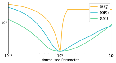
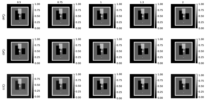
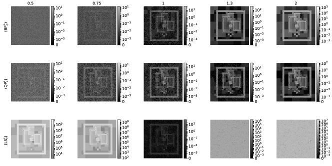
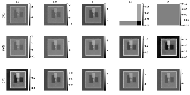
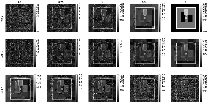
In Figure 11 and Figure 12 we depict estimator performance by visualizing the solution to each program at specific values of the normalized parameter. The description of each figure is identical, but the noise levels $\eta$ differ between them. Specifically, for each program we show the recovered image and its pixel-wise nnse for values of the normalized parameter $\rho=0.5,0.75,1,4/3,2$. The plot in the top row of the figure depicts a loss curve for each program (i.e., a curve generated from one realization of the noise $z$), along with reference lines for the corresponding values of the normalized parameter whose recovered image are visualized. The middle row contains a grid of 15 images; each column corresponds to a value of the normalized parameter as denoted by the title heading, while each row corresponds to a proximal denoising program as denoted by the labels along the left-most $y$-axis. The bottom grouping of 15 images depicts the pixel-wise nnse, arranged identically to the middle row. Because the average loss curves were computed on a grid of $n$ logarithmically spaced points centered about the optimal parameter value, we do not visualize the recovered image for the exact values of $\rho$ given above, but for those values represented by the coloured points seen in the plot of the top row. These points are sufficiently close to the quoted values of $\rho$ so as to visualize the program behaviour all the same.

The numerics of Figure 11 occur in the low-noise regime $(\eta=10^{-5})$, and so, as expected, demonstrate parameter instability of $(\mathrm{LS}_{\tau}^{*})$. We note that pixel-wise nnse for $(\mathrm{BP}_{\sigma}^{*})$ is approximately $20$ times worse than $(\mathrm{QP}_{\lambda}^{*})$ when $\rho\approx 2$. Moreover, the pathologies (in the sense of pixel-wise nnse) of these latter two programs appear similar. We also observe that the pixel-wise nnse varies more greatly for $(\mathrm{BP}_{\sigma}^{*})$ than for $(\mathrm{QP}_{\lambda}^{*})$ as $\rho$ varies from $0.75$ to $4/3$. This is consistent with our theory for the behaviour of $(\mathrm{BP}_{\sigma}^{*})$ in the very sparse regime. The numerics of Figure 12 occur in the high-noise regime $(\eta=0.5)$. Failure of $(\mathrm{BP}_{\sigma}^{*})$ in the very sparse regime is seen from examining the solution itself. For example, when $\rho<1$, pixel values of the solution to $(\mathrm{BP}_{\sigma}^{*})$ may reach more than $2$ or even be negative. This pathology manifests as large-magnitude pixelation in the corresponding plots of pixel-wise nnse. Catastrophic failure of $(\mathrm{BP}_{\sigma}^{*})$ is observed for $\rho>1$, in which the program fails to recover any semblance of the original image. Specifically, large $\sigma$ shrinks the wavelet coefficients to near the origin, enforcing few non-zero components that are small in magnitude. This yields the rectangular pattern observed in the solutions for $(\mathrm{BP}_{\sigma}^{*})$ (top-right of the middle row). In contrast, moderate deformation of the image is observed for $\rho\neq 1$ for both $(\mathrm{QP}_{\lambda}^{*})$ and $(\mathrm{LS}_{\tau}^{*})$.

Figure 10: Top (left-to-right): The underlying signal is the $640\times 640$ Square Shepp-Logan phantom image; the middle image is corrupted by iid normally distributed noise ($\eta=10^{-5}$); the right-most image is corrupted by iid normally distributed noise ($\eta=0.5$). The pixel values of the original image lie in $[0,1]$; those of the noisy images are scaled to $[0,1]$. Bottom: Average loss is plotted with respect to the normalized parameter for $(\mathrm{LS}_{\tau}^{*})$, $(\mathrm{QP}_{\lambda}^{*})$ and $(\mathrm{BP}_{\sigma}^{*})$ respectively when $\eta=10^{-5}$ (left) and $\eta=0.5$ (right). The associated parameters are $(s,N,k,n)=(5188,409618,25,501)$, implying relative sparsity of $1.27\%$. Plotted lines are smoothed approximations of loss realization data using multiquadric RBFs.

Figure 11: Wavelet space denoising of the square Shepp-Logan phantom for different values of the normalized parameter when $\eta=10^{-5}$. Top: The sections of the average-loss surface for which estimator recovery will be visualized are depicted by the dots which lie nearly on the blacked dotted lines, themselves located at $\rho=0.5,0.75,1,4/3,2$. Middle: This group of fifteen plots represents a program’s solution for a particular value of the normalized parameter, arranged in a grid. Image pixel values are not scaled to $[0,1]$; their range is given by the associated colour bar. Bottom: This group of fifteen plots depicts pixel-wise nnse for each (program, normalized parameter) pairing. In both the middle and bottom groups, the program is denoted along the left-hand side, while the normalized parameter value is denoted along the top row of each group.

Figure 12: Wavelet space denoising of the square Shepp-Logan phantom for different values of the normalized parameter when $\eta=0.5$. Top: The sections of the average-loss surface for which estimator recovery will be visualized are depicted by the dots which lie nearly on the blacked dotted lines, themselves located at $\rho=0.5,0.75,1,4/3,2$. Middle: This group of fifteen plots represents a program’s solution for a particular value of the normalized parameter, arranged in a grid. Image pixel values are not scaled to $[0,1]$; their range is given by the associated colour bar. Bottom: This group of fifteen plots depicts pixel-wise nnse for each (program, normalized parameter) pairing. In both the middle and bottom groups, the program is denoted along the left-hand side, while the normalized parameter value is denoted along the top row of each group.

7.5.4 Lasso Example

This section includes a realistic example comparing parameter instability of Lasso programs in the very sparse regime, both in the low noise regime and when the noise is relatively large. Specifically, we assume the model

$$y=Ax_{0}+z,\qquad x_{0}=\mathcal{W}(I)$$

where $\mathcal{W}(I)$ connotes the 2D Haar wavelet transform of $I$, the $80\times 80$ square Shepp-Logan phantom. This image size was reduced from that of section 7.5.3, because using the full image for the examples in this section would have been computationally prohibitive. The measurement matrix $A\in\mathbb{R}^{m\times N}$ has entries $A_{ij}\overset{\text{iid}}{\sim}Z/\sqrt{m}$ where $Z\sim\mathcal{N}(0,1)$. The parameters for the problem are $(N,s,m)=(6418,416,3110)$, implying a sparsity ratio of $6.48\%$ in the Haar wavelet domain, and a measurement matrix aspect ratio of $48.46\%$ with $m\gtrsim s\log(N/s)$. The wavelet coefficients $x_{0}$ are recovered according to $(\mathrm{LS}_{\tau,K})$, $(\mathrm{BP}_{\sigma,K})$ and $(\mathrm{QP}_{\lambda,K})$ where $K=B_{1}^{N}$.

Figure 13: Average loss (top) and average psnr (bottom) vs. normalized parameter for $(\mathrm{LS}_{\tau,K})$, $(\mathrm{QP}_{\lambda,K})$ and $(\mathrm{BP}_{\sigma,K})$ respectively when $\eta=2\cdot 10^{-3}$ (left) and $\eta=0.5$ (right). Associated parameters: $(s,N,m,k,n)=(416,6418,3110,25,301)$; relative sparsity $6.48\%$, aspect ratio $48.46\%$. Plotted lines approximate average of realization data using multiquadric RBFs.

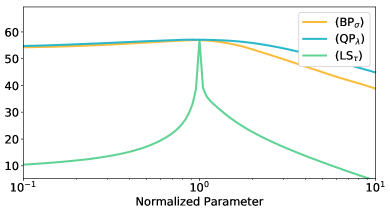
Given two signals $x^{*},x_{0}$ define the peak signal-to-noise ratio (psnr) by

$$\mathrm{psnr}(x^{*},x):=10\log_{10}\Big{(}\frac{\max_{i\in[N]}x_{i}^{2}}{\mathrm{mse}(x^{*},x_{0})}\Big{)},\qquad\mathrm{mse}(x^{*},x_{0}):=\frac{1}{N}\sum_{i=1}^{N}(x^{*}_{i}-x_{i})^{2}.$$ (4)

As with defining loss $L(\rho;x_{0},N,\eta\hat{z}_{ij})$, by abuse of notation we define psnr as a function of the normalized parameter $\rho$, $\mathrm{psnr}(\rho):=\mathrm{psnr}(\rho;x_{0},N,\eta\hat{z}_{ij}):=\mathrm{psnr}(x^{*}(\varrho),x_{0})$.

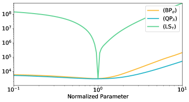
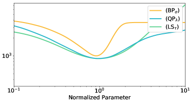
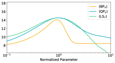
In Figure 13, we compute average loss and average psnr as a function of the normalized parameter, where average loss is measured using nnse in the image domain, as in section 7.5.3 and average psnr is defined as in (4). The data was simulated for $k=25$ realizations of noise for both $\eta=2\cdot 10^{-3}$ (left) and $\eta=0.5$ (right). Each curve visualized is a radial basis function approximation to the true average curve, obtained from the non-uniformly spaced point cloud of realization data. Specifically, the loss and psnr for each realization was computed on a logarithmically spaced grid of $n=301$ points about the optimal normalized parameter. For both average psnr and average loss, the resultant point cloud of $7\,525$ points for each program was used as input for a multiquadric RBF approximation with parameters $(\varepsilon_{\mathrm{rbf}},\mu_{\mathrm{rbf}},n_{\mathrm{rbf}})=(10^{-1},10,301)$ (except for $(\mathrm{LS}_{\tau,K})$ when $\eta=2\cdot 10^{-3}$, for which the parameters were $(\varepsilon_{\mathrm{rbf}},\mu_{\mathrm{rbf}},n_{\mathrm{rbf}})=(10^{-3},20^{-1},301)$, selected so as to properly resolve the cusp about $\rho=1$) [25].

About the optimal choice of normalized parameter, $\rho=1$, an approximate $1.51\cdot 10^{5}$ fold difference in average loss results from a $2.73\%$ average perturbation of the normalized parameter for $(\mathrm{LS}_{\tau,K})$ in the low-noise regime ($\eta=2\cdot 10^{-3}$). In contrast, the error difference is no more than $10^{3}$ for the other two programs. In particular, $(\mathrm{LS}_{\tau,K})$ undergoes an approximate $30\,\mathrm{dB}$ drop in psnr for this small variation. In the very sparse regime with $\eta=0.5$ (right), one observes that $(\mathrm{BP}_{\sigma,K})$ is the least stable when compared with the other two programs. If $\sigma$ is $10\%$ larger than the optimal choice, the psnr is approximately halved. Moreover, its best average loss is observed to be strictly greater than that for either of the other two programs. This observation mirrors the numerics for $(\mathrm{BP}_{\sigma}^{*})$ in section 7.5.3 and is consistent with the theoretical results of section 6.

Finally, we observe that the numerics for $(\mathrm{QP}_{\lambda,K})$ exhibit parameter stability, though the data regime is low-noise and very sparse (Figure 13, left). We claim this behaviour is not contrary to 5.2, and use the following intuition from $(\mathrm{QP}_{\lambda}^{*})$ to elucidate. When $\lambda<\bar{\lambda}$, Theorem 5.5 demonstrates parameter instability for $(\mathrm{QP}_{\lambda}^{*})$ behaving as $R^{\sharp}(\lambda;s,N)\gtrsim N^{\varepsilon}$ where $\lambda=(1-\varepsilon)\bar{\lambda}$. This term dominates $R^{\sharp}(\lambda;s,N)$ only for relatively high dimensional problems (cf. section 7.2), roughly requiring that $N^{\varepsilon}\gtrsim s\log(N/s)$. By this heuristic, in the present example, the instability does not dominate for $\varepsilon\leq C\cdot 0.80$ where $C>1$ is a constant. In particular, the theoretical results of 5.2 show that in high dimensions, if the signal is very sparse and the noise level is small, then $(\mathrm{QP}_{\lambda}^{*})$ is an appropriate choice only if $\lambda>\bar{\lambda}$, while our numerics support that $\lambda<\bar{\lambda}$ remains a safe choice for $(\mathrm{QP}_{\lambda}^{*})$ (cf. section 7.5.3) and $(\mathrm{QP}_{\lambda,K})$ in relatively lower dimensional problems. This observation is particularly advantageous given that parameter instability may still be expected of both $(\mathrm{LS}_{\tau,K})$ and $(\mathrm{BP}_{\sigma,K})$.

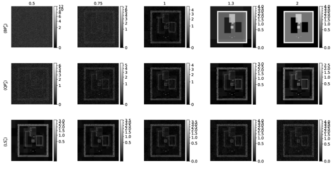
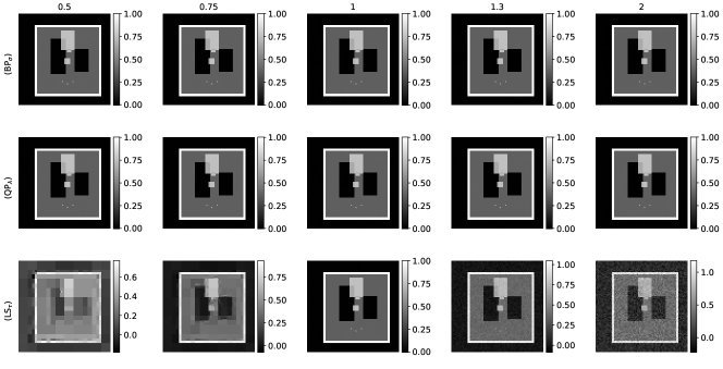
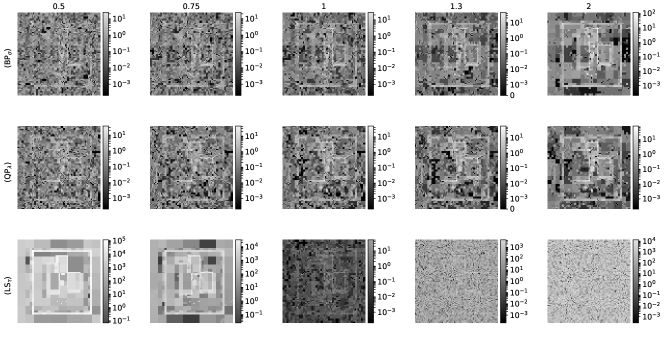
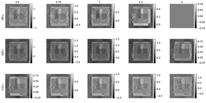
In Figure 14 and Figure 15, a grid of plots similar to those of section 7.5.3 were generated to visualize the solution to each program as a function of the normalized parameter $\rho\in\{0.5,0.75,1,4/3,2\}$. As before, the topmost image in each figure is a reference plot to depict the locations on the curve to which the displayed images correspond; however, these plots now depict psnr as a function of the normalized parameter. The images displayed below the reference plot do not correspond exactly to the quoted normalized parameters, but to a closest approximation obtained from a logarithmically spaced grid of $n=301$ points centered about the optimal parameter. These true normalized parameter values are visualized as large coloured dots on the reference plot; that they approximate well the quoted normalized parameter values for $\rho$ is verified by their proximity to the black dotted lines in the reference plot. Showing the estimator corresponding to a normalized parameter has the twofold purpose of visualizing the pathology of each program as its parameter varies, and demonstrating when a program is relatively unstable in a given regime.

The images in Figure 14 portray the setting of low-noise regime, with $\eta=2\cdot 10^{-3}$. Indeed, the reference plot displays a cusp for the $(\mathrm{LS}_{\tau,K})$ loss that was characteristic of $(\mathrm{LS}_{\tau}^{*})$ in the low-noise regime. Moreover, one observes similar pathologies in both the recovered image for $(\mathrm{LS}_{\tau,K})$ as well as the point-wise nnse. The image recovered using $(\mathrm{LS}_{\tau,K})$ is blurry for $\rho<1$, which is indicative of incompletely recovered wavelet coefficients. For $\rho>1$, the noise was not suppressed on the off-support of the wavelet coefficients yielding a noisy pixelated image in both the recovered image and the error image. This behaviour is observed to a significantly lesser degree for the corresponding $(\mathrm{BP}_{\sigma,K})$ and $(\mathrm{QP}_{\lambda,K})$ images.

The images in Figure 15 portray the very sparse regime where $\eta=0.5$. As is consistent with the asymptotics in section 6 for $(\mathrm{BP}_{\sigma}^{*})$, it is difficult to visualize $(\mathrm{BP}_{\sigma,K})$ parameter instability for relatively low dimensional problems. We suspect that this instability would have been markedly more apparent were it possible to run these simulations for the full $640\times 640$ square Shepp-Logan phantom image. Nevertheless, one observes that $(\mathrm{BP}_{\sigma,K})$ is the least stable of the three programs for $\rho>1$. In particular, the visualized estimator and point-wise nnse both depict catastrophic failure of $(\mathrm{BP}_{\sigma,K})$ for $\rho=2$.

Lastly, it is readily observed that the curves computed from single realizations resemble very closely those computed to approximate the average of several realizations. Notably, the nnse curves in Figure 14 and Figure 15 strongly resemble the corresponding average nnse curves in Figure 13.

Figure 14: Wavelet space compressed sensing problem with the square Shepp-Logan phantom for different values of the normalized parameter when $(s,N,m,\eta)=(416,6418,3110,2\cdot 10^{-3})$. Top: The sections of the psnr surface for which estimator recovery will be visualized are depicted by the dots which lie nearly on the black dotted lines, themselves located at $\rho=0.5,0.75,1,4/3,2$. Middle: This first $3\times 5$ group of plots shows each program’s solution for a particular value of the normalized parameter. Pixel values in an image are associated to its colour bar. Bottom: This $3\times 5$ group of plots depicts pixel-wise nnse for each (program, parameter) pairing. The program is denoted along the left-hand side, while the normalized parameter value is denoted along top row.

Figure 15: Wavelet space compressed sensing problem with the square Shepp-Logan phantom for different values of the normalized parameter when $(s,N,m,\eta)=(416,6418,3110,0.5)$. Top: The sections of the psnr surface for which estimator recovery will be visualized are depicted by the dots which lie nearly on the black dotted lines, themselves located at $\rho=0.5,0.75,1,4/3,2$. Middle: This first $3\times 5$ group of plots shows each program’s solution for a particular value of the normalized parameter. Pixel values in an image are associated to its colour bar. Bottom: This $3\times 5$ group of plots depicts pixel-wise nnse for each (program, parameter) pairing. The program is denoted along the left-hand side, while the normalized parameter value is denoted along top row.

8 Proofs

8.1 Proof of worst-case risk equivalence

Lemma 8.1 (Increasing risk).

Fix $x_{0}\in\Sigma_{s}^{N}$, $\|x_{0}\|_{1}=1$. Then $\hat{R}(\tau;\tau x_{0},N,\eta)$ is an increasing function of $\tau\geq 0$.

Proof 8.2 (Proof of Lemma 8.1).

Given $y(\tau):=\tau x_{0}+\eta z$ for $\eta>0$ and $z\in\mathbb{R}^{N},z_{i}\overset{\text{iid}}{\sim}\mathcal{N}(0,1)$, let $\hat{x}(\tau):=\hat{x}(\tau;y(\tau))$ solve

$$\hat{x}(\tau;y(\tau)):=\operatorname*{\arg\min}_{x}\{\|y(\tau)-x\|_{2}:\|x\|_{1}\leq\tau\}$$

Let $K:=B_{1}^{N}-x_{0}$, a convex set containing the origin. Using a standard scaling property of orthogonal projections,

$$\hat{x}(\tau)-x_{0} =\operatorname*{\arg\min}_{w}\{\|\eta z-w\|_{2}:\|w+\tau x_{0}\|_{1}\leq\tau\}$$

$$=\mathrm{P}_{\tau K}(\eta z).$$

Hence, it follows by Lemma 3.6 that $\|\hat{x}(\tau)-\tau x_{0}\|_{2}$ is an increasing function of $\tau$.

Proposition 8.3 (Risk equivalence).

Let $\eta,\tau>0$ and fix $N\geq 2$. Then

$$\sup_{x\in\Sigma_{s}^{N}}\hat{R}(\|x\|_{1};x,N,\eta)=\max_{\begin{subarray}{c}x\in\Sigma_{s}^{N}\\ \|x\|_{1}=1\end{subarray}}\lim_{\tau\to\infty}\hat{R}(\tau;\tau x,N,\eta)=\max_{\begin{subarray}{c}x\in\Sigma_{s}^{N}\\ \|x\|_{1}=1\end{subarray}}\lim_{\eta\to 0}\hat{R}(1;x,N,\eta).$$

Proof 8.4 (Proof of Proposition 8.3).

The first equality is an immediate consequence of Lemma 8.1:

$$\sup_{x\in\Sigma_{s}^{N}}\hat{R}(\|x\|_{1};x,N,\eta)=\max_{\begin{subarray}{c}x\in\Sigma_{s}^{N}\\ \|x\|_{1}=1\end{subarray}}\sup_{\tau>0}\hat{R}(\tau;\tau x,N,\eta)=\max_{\begin{subarray}{c}x\in\Sigma_{s}^{N}\\ \|x\|_{1}=1\end{subarray}}\lim_{\tau\to\infty}\hat{R}(\tau;\tau x,N,\eta).$$

The second equality follows from a standard property of orthogonal projections, and the risk expression derived in Lemma 8.1. For $K:=B_{1}^{N}-x$,

$$\max_{\begin{subarray}{c}x\in\Sigma_{s}^{N}\\ \|x\|_{1}=1\end{subarray}}\lim_{\tau\to\infty}\hat{R}(\tau;\tau x,N,\eta) =\max_{\begin{subarray}{c}x\in\Sigma_{s}^{N}\\ \|x\|_{1}=1\end{subarray}}\lim_{\tau\to\infty}\eta^{-2}\|\mathrm{P}_{\tau K}(\eta z)\|_{2}^{2}=\max_{\begin{subarray}{c}x\in\Sigma_{s}^{N}\\ \|x\|_{1}=1\end{subarray}}\lim_{\tau\to\infty}\frac{\tau^{2}}{\eta^{2}}\|\mathrm{P}_{K}(\tau^{-1}\eta z)\|_{2}^{2}$$

$$=\max_{\begin{subarray}{c}x\in\Sigma_{s}^{N}\\ \|x\|_{1}=1\end{subarray}}\lim_{\tilde{\eta}\to 0}\tilde{\eta}^{-2}\|\mathrm{P}_{K}(\tilde{\eta}z)\|_{2}^{2}=\max_{\begin{subarray}{c}x\in\Sigma_{s}^{N}\\ \|x\|_{1}=1\end{subarray}}\lim_{\eta\to 0}\hat{R}(1;x,N,\eta).$$

8.2 Proof of $(\mathrm{LS}_{\tau}^{*})$ optimal risk

Proof 8.5 (Proof of Proposition 2.5).

Directly from Theorem 3.1,

$$R^{*}(s,N)=\max_{\begin{subarray}{c}x_{0}\in\Sigma_{s}^{N}\\ \|x_{0}\|_{1}=1\end{subarray}}\mathbf{D}(T_{B_{1}^{N}}(x_{0})^{\circ})$$

where $\mathbf{D}(T_{B_{1}^{N}}(x_{0})^{\circ})$ is the mean-squared distance to the polar of the $\ell_{1}$ descent cone. The operator $\mathbf{D}$ has the following desirable relation to the Gaussian mean width, where $\mathcal{C}$ is a non-empty convex cone [2, Prop 10.2]:

$$w^{2}(\mathcal{C}\cap\mathbb{S}^{N-1})\leq\mathbf{D}(C^{\circ})\leq w^{2}(\mathcal{C}\cap\mathbb{S}^{N-1})+1.$$

Thus, it suffices to lower- and upper-bound $w^{2}\big{(}T_{B_{1}^{N}}\cap\mathbb{S}^{N-1}\big{)}$. The desired upper bound is an elementary but technical exercise using Hölder’s inequality, Stirling’s approximation and a bit of calculus. The lower bound may be computed using Sudakov’s inequality and [21, Lemma 10.12]. It thereby follows that

$$cs\log(N/s)\leq\mathbf{D}(T_{B_{1}^{N}}(x_{0})^{\circ})\leq Cs\log(N/s).$$

where $c,C>0$ are universal constants. Accordingly, $cs\log(N/s)\leq R^{*}(s,N)\leq Cs\log(N/s)$.

From Theorem 5.8, $R^{\sharp}(\lambda^{*};s,N)\leq Cs\log N$ for any $N\geq N_{0}(s)$ with $N_{0}(s)$ sufficiently large. Using the above equation gives, for $c,C_{1}>0$, $Cs\log N\leq C_{1}cs\log(N/s)\leq C_{1}R^{*}(s,N)$. Finally, observe that $R^{\sharp}(\lambda^{*};s,N)$ is trivially lower bounded by $M^{*}(s,N)=\Theta(s\log(N/s))$ [9].

8.3 Proof of $\ell_{1}$ tangent cone equivalence

Proof 8.6 (Proof of Lemma 3.5).

First observe that the definition of $F_{\mathcal{C}}(x)$ is equivalent to

$$F_{\mathcal{C}}(x)=\{h\in\mathbb{R}^{N}:h=z-x,\,\|z\|_{1}\leq\|x\|_{1}\}.$$

Next, observe that $K(x)$ is a cone. So, for left containment, it suffices to show $F_{\mathcal{C}}(x)\subseteq K(x)$ since the cone generated by a set is no larger than any cone containing that set. These two expressions:

$$\langle\mathrm{sgn}(x)_{T},x\rangle =\|x\|_{1}\geq\|z\|_{1}=\|z_{T}\|_{1}+\|h_{T^{C}}\|_{1}$$

$$\|z_{T}\|_{1} =\langle\mathrm{sgn}(z),z_{T}\rangle\geq\langle\mathrm{sgn}(x),z_{T}\rangle,$$

are by definition of $h=z-x\in F_{\mathcal{C}}(x)$. They combine to yield left containment:

$$\|h_{T^{C}}\|_{1}\leq-\langle\mathrm{sgn}(x),z_{T}-x\rangle=-\langle\mathrm{sgn}(x),h_{T}\rangle=-\langle\mathrm{sgn}(x),h\rangle.$$

To show right containment, first fix $w\in K(x)$ and select $\alpha\geq 0$ sufficiently small so that $z:=x+\alpha w$ admits $z_{j}x_{j}\geq 0$ for all $j\in T$. Using $\alpha\|w_{T^{C}}\|_{1}\leq-\alpha\langle\mathrm{sgn}(x),w_{T}\rangle$, we show $\|z\|_{1}\leq\|x\|_{1}$ implying that $\alpha w\in F_{\mathcal{C}}(x)$, whence $w\in T_{\mathcal{C}}(x)$. Where $h:=\alpha w=z-x$,

$$\|z\|_{1} =\|z_{T}\|_{1}+\|z_{T^{C}}\|_{1}=\langle\mathrm{sgn}(z_{T}),z_{T}\rangle+\|h_{T^{C}}\|_{1}$$

$$\leq\langle\mathrm{sgn}(z_{T}),z_{T}\rangle-\langle\mathrm{sgn}(x),h_{T}\rangle=\langle\mathrm{sgn}(z_{T}),z_{T}\rangle-\langle\mathrm{sgn}(x),h_{T}\rangle+\langle\mathrm{sgn}(x),x\rangle-\langle\mathrm{sgn}(x),x\rangle$$

$$=\langle\mathrm{sgn}(x),x\rangle+\langle\mathrm{sgn}(z_{T}),z_{T}\rangle-\langle\mathrm{sgn}(x),z_{T}\rangle=\|x\|_{1}+\langle\mathrm{sgn}(z_{T})-\mathrm{sgn}(x),z_{T}\rangle=\|x\|_{1}$$

where the latter equality follows from the fact that $\langle\mathrm{sgn}(z_{T})-\mathrm{sgn}(x),z_{T}\rangle\neq 0$ only if $x_{j}z_{j}<0$ for some $j\in T$, which goes against the initial assumption defining $\alpha$ and $z$. Thus, $w\in T_{\mathcal{C}}(x)$ and $T_{\mathcal{C}}(x)=K(x)$ as desired.

8.4 Proof of the projection lemma

Proof 8.7 (Proof of Lemma 3.6).

Define $z_{\alpha}:=\mathrm{P}_{\alpha K}(z)$ for $\alpha=1,\lambda$ and define $f(t):=\|u_{t}\|_{2}^{2}$, where $u_{t}:=tz_{\lambda}+(1-t)z_{1}$ for $t\in[0,1]$. Our goal is to show $\left.\frac{\mathrm{d}}{\mathrm{d}t}\right|_{t=0}f(t)\geq 0$; this implies $\|z_{\lambda}\|_{2}\geq\|z_{1}\|_{2}$, because $f$ is convex. Expanding $f(t)$,

$$f(t) =t^{2}\big{(}(\|z_{\lambda}\|_{2}^{2}-2\langle z_{1},z_{\lambda}\rangle+\|z_{1}\|_{2}^{2}\big{)}+2t\big{(}\langle z_{1},z_{\lambda}\rangle-\|z_{1}\|_{2}^{2}\big{)}+\|z_{1}\|_{2}^{2}.$$

So it is required to check the condition $(\star)$:

$$\left.\frac{\mathrm{d}}{\mathrm{d}t}f(t)\right|_{t=0} =\left[2t\|z_{\lambda}-z_{1}\|_{2}^{2}+2\langle z_{1},z_{\lambda}-z_{1}\rangle\right|_{t=0}=2\langle z_{1},z_{\lambda}-z_{1}\rangle\overset{(\star)}{\geq}0$$

The projection condition says that if $\mathrm{P}_{C}(x)$ is the projection of $x$ onto a convex set $C$ then for any $y\in C$, $\langle y-\mathrm{P}_{C}(x),x-\mathrm{P}_{C}(x)\rangle\leq 0$. From the projection condition [6], we have

• $\langle\lambda^{-1}z_{\lambda}-z_{1},z-z_{1}\rangle\leq 0$

• $\langle\lambda z_{1}-z_{\lambda},z-z_{\lambda}\rangle\leq 0$.

Accordingly,

$$0 \geq\langle z_{\lambda}-\lambda z_{1},z-z_{1}\rangle+\langle\lambda z_{1}-z_{\lambda},z-z_{\lambda}\rangle$$

$$=\langle\lambda z_{1}-z_{\lambda},z_{1}-z_{\lambda}\rangle=\langle(\lambda-1)z_{1},z_{1}-z_{\lambda}\rangle+\|z_{1}-z_{\lambda}\|_{2}^{2}$$

$$\geq(\lambda-1)\langle z_{1},z_{1}-z_{\lambda}\rangle$$

which is equivalent to $\langle z_{1},z_{\lambda}-z_{1}\rangle\geq 0$. Therefore, $f$ is a convex function increasing on the interval $t\in[0,1]$, whence $\|z_{1}\|_{2}\leq\|z_{\lambda}\|_{2}$ as desired.

Remark 8.8.

There is a simpler way to begin the proof of the projection lemma. To show

$$\|z_{1}\|_{2}\leq\|z_{\lambda}\|_{2}\quad\iff\quad\|z_{1}\|_{2}^{2}\leq\|z_{1}\|_{2}\|z_{\lambda}\|_{2},$$

one may instead prove the following chain,

$$\|z_{1}\|_{2}^{2}\leq\langle z_{1},z_{\lambda}\rangle\leq\|z_{1}\|_{2}\|z_{\lambda}\|_{2}.$$

The latter inequality is true by Cauchy-Schwarz, so it remains only to prove the former:

$$\langle z_{1},z_{\lambda}\rangle-\|z_{1}\|_{2}^{2}\geq 0\quad\iff\quad\langle z_{1},z_{\lambda}-z_{1}\rangle\geq 0.$$

Rearranging shows this inequality is equivalent to $(\star)$, and the remainder of the proof proceeds as is. This remark is included for intuition, but this approach is less generalizable. For example, it does not yield the rate of growth observed in the remark at the end of 3.1.1.

8.5 Elementary results from probability

We briefly recall two aspects of how normal random vectors concentrate in high dimensions.

Proposition 8.9.

Let $z\in\mathbb{R}^{N}$ with $z_{i}\overset{\text{iid}}{\sim}\mathcal{N}(0,1)$, fix constants $0<C_{2}<C_{1}<\infty$ and define the event $\mathcal{Z}_{\pm}$ by $\mathcal{Z}_{\pm}:=\{C_{2}\sqrt{2N}\leq\|z\|_{2}^{2}-N\leq C_{1}\sqrt{2N}\}$. There exists a constant $p=p(C_{1},C_{2})>0$ and integer $N_{0}\geq 1$ such that for all $N\geq N_{0}$,

$$\mathbb{P}\big{(}\mathcal{Z}_{\pm}\big{)}\geq p$$

Proof 8.10 (Proof of Proposition 8.9).

Define the $\chi^{2}_{N}$-distributed random variable

$$X_{N}:=\frac{\|z\|_{2}^{2}-N}{\sqrt{2N}}.$$

Since $X_{N}\xrightarrow{N\to\infty}\mathcal{N}(0,1)$ by the central limit theorem, for any $\varepsilon>0$ there is $N_{0}\in\mathbb{N}$ such that

$$\big{|}\mathbb{P}\big{(}X_{N}\leq t\big{)}-\Phi(t)\big{|}\leq\varepsilon$$

for all $N\geq N_{0}$, where $\Phi$ is the standard normal cdf. One need merely choose $\varepsilon>0$ so that

$$\mathbb{P}\big{(}\mathcal{Z}_{\pm}\big{)}\geq\Phi(C_{2})-\Phi(C_{1})-2\varepsilon=:p(C_{1},C_{2})>0$$

and choose the first $N_{0}$ for which the chain of inequalities is valid for all $N\geq N_{0}$.

Corollary 8.11.

Fix $N,N_{0}\in\mathbb{N}$ with $N\geq N_{0}\geq 2$. Let $z\in\mathbb{R}^{N}$ with $z_{i}\overset{\text{iid}}{\sim}\mathcal{N}(0,1)$ and define the event

$$A_{N}:=\big{\{}\|z\|_{2}^{2}\leq N-2\sqrt{N}\quad\And\quad\|z\|_{\infty}\leq\sqrt{3\log N}\big{\}}$$

There exists a real constant $C=C(N_{0})>0$ such that $\mathbb{P}(A_{N})\geq C$.

Proof 8.12 (Proof of Corollary 8.11).

Given $N$, define the events $E_{N}:=\{\|z\|_{2}^{2}\leq N-2\sqrt{N}\}$ and $F_{N}:=\{\|z\|_{\infty}\leq\sqrt{3\log N}\}$. Using the standard identity $\Phi(-x)\leq\phi(x)/x$, we note that

$$\mathbb{P}(F_{N})\geq 1-2N\mathbb{P}(|Z|>\sqrt{3\log N})\geq 1-\frac{2}{\sqrt{\frac{3}{2}\pi N_{0}\log N_{0}}}>0$$

With this, and a standard argument similar to that of Proposition 8.9, one may show

$$\mathbb{P}(A_{N})=\mathbb{P}(E_{N}F_{N})=\mathbb{P}(E_{N}\mid F_{N})\mathbb{P}(F_{N})\geq\mathbb{P}(E_{N})\mathbb{P}(F_{N})\geq C\geq 0.$$

We also recall that an event holding with high probability, intersected with an event occurring with constant probability, still occurs with constant probability.

Proposition 8.13.

Let $N\geq 1$ be an integer and suppose that $\mathcal{E}=\mathcal{E}(N)$ is an event that holds with high probability in the sense that

$$\mathbb{P}(\mathcal{E}_{N})\geq 1-p(N)$$

for some function $p(N)>0$ with $\lim_{N\to\infty}p(N)=0$. Suppose also that for an event $\mathcal{F}=\mathcal{F}(N)$ there exists $q>0$ such that $\inf_{N\geq 1}\mathbb{P}(\mathcal{F}(N))\geq q$. Then there exists a constant $q^{\prime}>0$ and integer $N_{0}\geq 1$ such that $\mathbb{P}\big{(}\mathcal{E}(N)\cap\mathcal{F}\big{)}\geq q^{\prime}$ for all $N\geq N_{0}$.

Proof 8.14 (Proof of Proposition 8.13).

The proof is very similar to that of Proposition 8.9. Simply choose a threshold $\varepsilon>0$ and select the first $N_{0}\geq 1$ for which

$$\mathbb{P}\big{(}\mathcal{E}(N)\cap\mathcal{F}\big{)}\geq q-p(N)\geq q-\varepsilon=:q^{\prime}>0$$

for all $N\geq N_{0}$.

Remark 8.15.

An example of such a $p(N)$ as in Proposition 8.13 is $p(N)\sim O(e^{-N})$ when $\mathcal{E}_{N}:=\{|X-\mu|\leq t\}$ for $X$ a subgaussian random variable, $\mathbb{E}X=\mu$ and $t>0$.

8.6 Proof of $(\mathrm{LS}_{\tau}^{*})$ parameter instability

Proof 8.16 (Proof of Theorem 4.1).

Let $x_{0}\in\Sigma_{s}^{N}$ with non-empty support and let $\tau>0$ be the governing parameter of $(\mathrm{LS}_{\tau}^{*})$. First suppose the parameter is chosen smaller than the optimal value, i.e., $\tau<\|x_{0}\|_{1}$. The discrepancy of the guess, $\rho:=|\|x_{0}\|_{1}-\tau|=\|x_{0}\|_{1}-\tau>0$, induces the instability.

The solution $\hat{x}(\tau)$ to $(\mathrm{LS}_{\tau}^{*})$ satisfies $0\leq\|\hat{x}(\tau)\|_{1}\leq\tau$ by construction. Therefore, by the Cauchy-Schwarz inequality and an application of the triangle inequality,

$$\|\hat{x}(\tau)-x_{0}\|_{2}^{2}\geq N^{-1}\|\hat{x}(\tau)-x_{0}\|_{1}^{2}\geq\frac{\rho^{2}}{N}>0.$$

Accordingly,

$$\lim_{\eta\to 0}\frac{1}{\eta^{2}}\|\hat{x}(\tau)-x_{0}\|_{2}^{2}\geq\lim_{\eta\to 0}\frac{\rho^{2}}{N\eta^{2}}=\infty.$$

Next assume $\tau$ is chosen too large, with discrepancy between the correct and actual guesses for the parameter again being denoted $\rho=\tau-\|x_{0}\|_{1}>0$. Two key pieces of intuition guide this result. The first is that the error of approximation should be controlled by the effective dimension of the constraint set. The second suggests that $y$ continues to lie within the constraint set for sufficiently small noise level, meaning recovery behaves as though it were unconstrained. Hence, the effective dimension of the problem is that of the ambient dimension, and so one should expect the error to be proportional to $N$.

First, we show that for $\eta$ sufficiently small, $y\in\tau B_{1}^{N}$ with high probability. Fix a sequence $\eta_{j}\xrightarrow{j\to\infty}0$ and define $y_{j}:=x_{0}+\eta_{j}z$. Since $\|z\|_{1}$ is subgaussian, Theorem 3.10 implies there is a constant $C>0$ such that

$$\mathbb{P}\big{(}\|z\|_{1}\geq t+N\sqrt{\frac{2}{\pi}}\big{)}\leq\mathbb{P}\big{(}\big{|}\|z\|_{1}-N\sqrt{\frac{2}{\pi}}\big{|}\geq t\big{)}\leq e\cdot\exp\big{(}\frac{-t^{2}}{CN}\big{)}.$$

In order to satisfy $x_{0}+\eta z\in\tau B_{1}^{N}$, we need $\|x_{0}+\eta z\|_{1}<\tau$, for which $\eta\|z\|_{1}<\rho$ is sufficient. The probability that this event does not occur is upper bounded by

$$\mathbb{P}\big{(}\|z\|_{1}\geq\frac{\rho}{\eta}\big{)}\leq\mathbb{P}\big{(}\|z\|_{1}\geq t+N\sqrt{\frac{2}{\pi}}\big{)}\leq e\cdot\exp\big{(}-\frac{t^{2}}{CN}\big{)}$$

For $t=\rho/\eta-N\sqrt{\frac{2}{\pi}}$, and $\tilde{C}>0$ a new constant,

$$\mathbb{P}\left(\|z\|_{1}\geq\frac{\rho}{\eta}\right)\leq e\cdot\exp\left(-\frac{\big{(}\rho/\eta-N\sqrt{2/\pi}\big{)}^{2}}{CN}\right)\lesssim\tilde{C}\exp\left(-\frac{\rho^{2}}{N\eta^{2}}\right)\xrightarrow{\eta\to 0}0.$$

Let $E_{j}:=\{\|z\|_{1}<\displaystyle\frac{\rho}{\eta_{j}}\}$ for $j\geq 1$; their respective probabilities lower-bounded by $p_{j}:=1-\tilde{C}\exp(-\rho^{2}/N\eta_{j}^{2})$. Given $0<\varepsilon\ll 1$, denote by $j_{0}$ the first integer such that $p_{j}\geq 1-\varepsilon$ for all $j\geq j_{0}$. On $E_{j}$ with $j\geq j_{0}$, $y_{j}\in\tau B_{1}^{N}$ so $y_{j}$ is the unique minimizer of $(\mathrm{LS}_{\tau}^{*})$, meaning:

$$\frac{1}{\eta^{2}}\|\hat{x}(\tau)-x_{0}\|_{2}^{2}=\|z\|_{2}^{2}.$$

The result follows by bounding the following expectations:

$$\lim_{\eta\to 0}\frac{1}{\eta^{2}}\mathbb{E}\|\hat{x}(\tau)-x_{0}\|_{2}^{2}=\lim_{j\to\infty}\mathbb{E}\big{[}\eta_{j}^{-2}\|\hat{x}(\tau)-x_{0}\|_{2}^{2}\operatorname{\mathbbm{1}}(E_{j})\big{]}+\mathbb{E}\big{[}\eta_{j}^{-2}\|\hat{x}(\tau)-x_{0}\|_{2}^{2}\operatorname{\mathbbm{1}}(E_{j}^{C})\big{]}. \star$$ ()

The first term converges by dominated convergence theorem:

$$\lim_{j\to\infty}\mathbb{E}\big{[}\eta_{j}^{-2}\|\hat{x}(\tau)-x_{0}\|_{2}^{2}\operatorname{\mathbbm{1}}(E_{j})\big{]}=\lim_{j\to\infty}\mathbb{E}\big{[}\operatorname{\mathbbm{1}}(E_{j})\|z\|_{2}^{2}\big{]}=\mathbb{E}\big{[}\|z\|_{2}^{2}\big{]}=N.$$

On $E_{j}^{C}$, $\|\hat{x}(\tau)-x_{0}\|_{2}^{2}\leq\|\hat{x}(\tau)-x_{0}\|_{1}^{2}\leq\rho^{2}\eta^{2}$, so by dominated convergence theorem,

$$\lim_{j\to\infty}\mathbb{E}\big{[}\eta_{j}^{-2}\|\hat{x}(\tau)-x_{0}\|_{2}^{2}\operatorname{\mathbbm{1}}(E_{j}^{C})\big{]}\leq\lim_{j\to\infty}\mathbb{E}\big{[}\|z\|_{1}^{2}\operatorname{\mathbbm{1}}(E_{j}^{C})\big{]}=0.$$

This immediately yields the desired result,

$$\lim_{\eta\to 0}\frac{1}{\eta^{2}}\mathbb{E}\|\hat{x}(\tau)-x_{0}\|_{2}^{2}=N.$$

To prove the final case where $\tau=\|x_{0}\|_{1}$, set $\mathcal{C}=B_{1}^{N}$ in (1) of Theorem Theorem 3.1. Then,

$$\lim_{\eta\to 0}\eta^{-2}\mathbb{E}\|\hat{x}(\tau)-x_{0}\|_{2}^{2}=\mathbf{D}(T_{\mathbb{B}_{1}^{N}}(x_{0})^{\circ})=\Theta(s\log(N/s))\ll N.$$

8.7 Proofs of $(\mathrm{QP}_{\lambda}^{*})$ results

Proof 8.17 (Proof of Proposition 5.1).

Because $z$ is isotropic and iid, one can split the signal $x_{0}=x_{0}^{+}-x_{0}^{-}$ into “positive” and “negative” components, and so it suffices to consider the case where $x_{0,j}\geq 0$ for all $j\in[N]$. The heart of this proposition again relies on the fact that the noise limits to $0$. In general, $\lambda>0$ is finite and typically small ($\sim\mathcal{O}(\eta\sqrt{\log N})$, so we require only that $|x_{0,j}|=\mathcal{O}(1)$ for $j\in T=\mathrm{supp}(x_{0})$. This requirement can be written $x_{0,j}\geq a>0$ for all $j\in T$ and some real number $a>0$. Recall that the minimizer of $(\mathrm{QP}_{\lambda}^{*})$ is given by the soft-thresholding operator which we denote by

$$x^{\sharp}(\eta\lambda)=S_{\eta\lambda}(x_{0}+\eta z).$$

Where $k\in T,\ell\in T^{C}$ so that $x_{0,k}\geq a$, $x_{0,\ell}=0$, one has

$$S_{\eta\lambda}(x_{0,k}+\eta z_{k})-x_{0,k} =\begin{cases}\eta(z_{k}-\lambda)&x_{0,k}>\eta(\lambda-z_{k})\\ -x_{0,k}&|x_{0,k}+\eta z_{k}|\leq\eta\lambda\\ \eta(z_{k}+\lambda)&x_{0,k}<-\eta(\lambda+z_{k})\end{cases} S_{\eta\lambda}(\eta z_{\ell}) =\begin{cases}\eta(z_{\ell}-\lambda)&z_{\ell}>\lambda\\ 0&|z_{\ell}|\leq\lambda\\ \eta(z_{\ell}+\lambda)&z_{\ell}<-\lambda\end{cases}$$

and so independence of $z_{j}$ yields

$$\lim_{\eta\to 0}\frac{1}{\eta^{2}}\mathbb{E}\|x^{\sharp}(\eta\lambda)-x_{0}\|_{2}^{2}=\lim_{\eta\to 0}\frac{s}{\eta^{2}}\mathbb{E}\big{[}(S_{\eta\lambda}(x_{0,k}+\eta z_{k})-x_{0,k})^{2}\big{]}+\lim_{\eta\to 0}\frac{N-s}{\eta^{2}}\mathbb{E}\big{[}S_{\eta\lambda}(z_{\ell})^{2}\big{]}.$$

Passing to a sequence $\eta_{j}\to 0$, there exists $J\in\mathbb{N}$ such that for all $j\geq J$,

$$S_{\eta_{j}\lambda}(x_{0,k}+\eta_{j}z_{k})-x_{0,k}=\eta_{j}(z_{k}-\lambda)\qquad\text{with high probability.} \star$$ ()

If this equality were true almost surely, it would follow that for $k\in T$

$$\eta^{-2}\mathbb{E}\|(x^{\sharp}(\eta\lambda)-x_{0})_{T}\|_{2}^{2}=\mathbb{E}\big{[}(z_{T}-\lambda)^{2}\big{]}=\mathbb{E}[z_{T}^{2}\big{]}+s\lambda^{2}=s(1+\lambda^{2}).$$

Indeed this is still true in the case of $(\star)$ with $\eta\to 0$. In particular, using independence of $z_{k}$ for $k\in T$ and denoting by $E_{j}$ the high probability event $(\star)$, we obtain by similar means as in the proof of Theorem 4.1,

$$\lim_{\eta\to 0}\eta^{-2}\mathbb{E}\|(x^{\sharp}(\eta\lambda)-x_{0})_{T}\|_{2}^{2} =\lim_{j\to\infty}\frac{s}{\eta_{j}^{2}}\mathbb{E}\big{[}\eta_{j}^{2}(z_{k}-\lambda)^{2}\operatorname{\mathbbm{1}}(E_{j})\big{]}+\frac{s}{\eta_{j}^{2}}\mathbb{E}\big{[}(x^{\sharp}_{k}(\eta_{j}\lambda)-x_{0,k})^{2}\operatorname{\mathbbm{1}}(E_{j}^{C})\big{]}=s(1+\lambda^{2})$$

Next, define $G(\lambda):=(1+\lambda^{2})\Phi(-\lambda)-\lambda\phi(\lambda)$. By independence of the entries of $z_{T^{C}}$, with any $\ell\in T^{C}$, the second quantity is exactly computable as

$$\lim_{\eta\to 0}\eta^{-2}\mathbb{E}\|(x^{\sharp}(\eta\lambda)-x)_{T^{C}}\|_{2}^{2}=(N-s)\mathbb{E}\big{[}S_{\lambda}(z_{\ell})^{2}\big{]}=2(N-s)G(\lambda),$$

where the final equality is by definition of $S_{\lambda}$ and elementary calculations (cf. remark remark 8.23). Therefore, as desired,

$$\lim_{\eta\to 0}\eta^{-2}\mathbb{E}\|x^{\sharp}(\eta\lambda)-x\|_{2}^{2}=s(1+\lambda^{2})+2(N-s)G(\lambda).$$

Proof 8.18 (Proof of Corollary 5.3).

For $0\leq t\leq s$, where we define for simplicity of notation $\Sigma_{-1}^{N}:=\emptyset$, observe that

$$\sup_{x_{0}\in\Sigma_{t}^{N}\setminus\Sigma_{t-1}^{N}}R^{\sharp}(\lambda;x_{0},N,\eta)=R^{\sharp}(\lambda;t,N)$$

because the regime $\eta\to 0$ is equivalent, by a rescaling argument, to the regime in which $\eta>0$ and $|x_{0,j}|\to\infty$ for $j\in\mathrm{supp}(x_{0})$ (as shown explicitly in the proof of Proposition 8.3). Therefore,

$$\sup_{x_{0}\in\Sigma_{s}^{N}}R^{\sharp}(\lambda;x_{0},N,\eta) =\max_{0\leq t\leq s}\sup_{x_{0}\in\Sigma_{t}^{N}\setminus\Sigma_{t-1}^{N}}R^{\sharp}(\lambda;x_{0},N,\eta)$$

$$=\max\{R^{\sharp}(\lambda;0,N),R^{\sharp}(\lambda;s,N)\}$$

$$=R^{\sharp}(\lambda;s,N)$$

by linearity of the $\max$ argument and the fact that $1+\lambda^{2}\geq G(\lambda)$ for $\lambda>0$.

8.7.1 Proof of $(\mathrm{QP}_{\lambda}^{*})$ parameter instability

We now prove Lemma Lemma 5.4.

Proof 8.19 (Proof of Lemma Lemma 5.4).

By Proposition Proposition 5.1, $R^{\sharp}(\lambda;s,N)=s(1+\lambda^{2})+2(N-s)G(\lambda)$. We prove the result by controlling $G^{\prime}(\lambda)$ using integration by parts. Thus,

$$\frac{\mathrm{d}}{\mathrm{d}\lambda}G(\lambda)=2\lambda\Phi(-\lambda)-2\phi(\lambda)\leq 2\lambda(\frac{1}{\lambda}-\frac{1}{\lambda^{3}}+\frac{3}{\lambda^{5}})\phi(\lambda)-2\phi(\lambda)=-2\frac{\lambda^{2}-3}{\lambda^{4}}\phi(\lambda)$$

A simple substitution yields, for all $N>\exp\Big{(}\frac{3}{2}(1-\varepsilon)^{-2}\Big{)}$,

$$\left.\frac{\mathrm{d}}{\mathrm{d}u}\right|_{u=1-\varepsilon}\hskip-22.0ptG(u\bar{\lambda}) \leq\left[-2\frac{(u\bar{\lambda})^{2}-3}{u^{4}\bar{\lambda}^{3}}\phi(u\bar{\lambda})\right|_{u=1-\varepsilon}=-\frac{2(1-\varepsilon)^{2}\log(N)-3}{(1-\varepsilon)^{4}\sqrt{\pi\log^{3}(N)}}N^{-(1-\varepsilon)^{2}}=:-\frac{1}{2}\gamma(N,\varepsilon)N^{-(1-\varepsilon)^{2}}.$$

Multiplying $G((1-\varepsilon)\bar{\lambda})$ by $N-s$ yields

$$\left|\frac{\mathrm{d}}{\mathrm{d}u}R^{\sharp}(u\bar{\lambda};s,N)\right|_{u=1-\varepsilon} \geq(N-s)\gamma(N,\varepsilon)N^{-(1-\varepsilon)^{2}}-2s(1-\varepsilon)\sqrt{2\log N}$$

$$=\gamma(N,\varepsilon)N^{2\varepsilon-\varepsilon^{2}}-s\gamma(N,\varepsilon)N^{-(1-\varepsilon)^{2}}-2s(1-\varepsilon)\sqrt{2\log N}$$

$$\geq CN^{\varepsilon}$$

for some constant $C>0$ under the condition that $N\geq N_{0}$, where $N_{0}>\exp\Big{(}\frac{3}{2}(1-\varepsilon)^{-2}\Big{)}$ is chosen so that for all $N\geq N_{0}$ the following two conditions are satisfied:

$$\begin{cases}(N-s)\gamma(N,\varepsilon)N^{-(1-\varepsilon)^{2}}\geq 2s(1-\varepsilon)\sqrt{2\log N}\\[7.11317pt] \gamma(N,\varepsilon)\big{(}1-\frac{s}{N}\big{)}\geq 2s(1-\varepsilon)N^{-2\varepsilon+\varepsilon^{2}}\sqrt{2\log N}+CN^{-\varepsilon+\varepsilon^{2}}\end{cases}$$

In this regime, one achieves unbounded growth of the risk as a power law of the ambient dimension.

Remark 8.20.

Using integration by parts, one has for $x>0$,

$$\Phi(-x) =\int_{x}^{\infty}\phi(t)\,\mathrm{d}t=\Big{(}\frac{1}{x}-\frac{1}{x^{3}}\Big{)}\phi(x)+3\int_{x}^{\infty}\frac{t\phi(t)}{t^{5}}\,\mathrm{d}t$$

$$\leq\Big{(}\frac{1}{x}-\frac{1}{x^{3}}\Big{)}\phi(x)+3x^{-5}\int_{x}^{\infty}t\phi(t)\,\mathrm{d}t=\Big{(}\frac{1}{x}-\frac{1}{x^{3}}+\frac{3}{x^{5}}\Big{)}\phi(x)$$

Proof 8.21 (Proof of Theorem 5.5).

Define $f(u):=\frac{\mathrm{d}}{\mathrm{d}u}R^{\sharp}(u\bar{\lambda};s,N)$ and $F(u):=R^{\sharp}(u\bar{\lambda};s,N)$ its anti-derivative. The proof is an application of the fundamental theorem of calculus:

$$F(1)-F(1-\varepsilon)=\int_{0}^{\varepsilon}f(1-t)\,\mathrm{d}t\leq-C\int_{0}^{\varepsilon}N^{t}\,\mathrm{d}t=C\frac{1-N^{\varepsilon}}{\log N}.$$

The result follows by substituting:

$$R^{\sharp}((1-\varepsilon)\bar{\lambda};s,N)\geq C\frac{N^{\varepsilon}-1}{\log N}+R^{\sharp}(\bar{\lambda};s,N)\geq C\frac{N^{\varepsilon}}{\log N}$$

where the latter inequality holds after taking $N$ sufficiently large, and $C>0$ is a universal constant that has changed values in the final expression.

Proof 8.22 (Proof of Proposition 5.6).

By Proposition 5.1, $R^{\sharp}(\lambda;s,N)=s(1+\lambda^{2})+2(N-s)G(\lambda)$. We prove the result by controlling $G^{\prime}(\lambda)$. One may lower bound $G^{\prime}(\lambda)$ as

$$\frac{\mathrm{d}}{\mathrm{d}\lambda}G(\lambda)=2\lambda\Phi(-\lambda)-2\phi(\lambda)\geq 2\lambda\Big{(}\frac{\lambda}{\lambda^{2}+1}\Big{)}\phi(\lambda)-2\phi(\lambda)=-2\frac{\phi(\lambda)}{\lambda^{2}+1}.$$

This gives the following lower bound for $\frac{\mathrm{d}}{\mathrm{d}\lambda}R^{\sharp}(\lambda;s,N)$:

$$\frac{\mathrm{d}R^{\sharp}}{\mathrm{d}\lambda}(\lambda;s,N)\geq 2s\lambda-4(N-s)\frac{\phi(\lambda)}{\lambda^{2}+1}\geq 2\lambda-4N\frac{\phi(\lambda)}{\lambda^{2}+1}=\frac{2}{\lambda^{2}+1}\big{(}\lambda(\lambda^{2}+1)-2N\phi(\lambda)\big{)}.$$

Substituting $\bar{\lambda}$ gives a positive quantity, since $N\geq 2$:

$$\frac{2}{2\log N+1}\big{(}\sqrt{2\log N}(2\log N+1)-\frac{2}{\sqrt{2\pi}}\big{)}>0.$$

Consequently, $\lambda^{*}<\bar{\lambda}$ because $\lambda^{*}$ is the value giving optimal risk and $\frac{\mathrm{d}}{\mathrm{d}\lambda}R^{\sharp}(\lambda;s,N)$ is increasing for all $\lambda\geq\bar{\lambda}$. Then it must be that $|\lambda^{*}-\bar{\lambda}|<\varepsilon$ for any $\varepsilon>0$ when $N$ is sufficiently large. Indeed, fix $\varepsilon>0$. By Lemma 5.4 there exists $N_{0}\geq 1$ so that for all $N\geq N_{0}$ $(\mathrm{QP}_{\lambda}^{*})$ is parameter unstable for $\lambda<\bar{\lambda}$, yielding $R^{\sharp}(\lambda;s,N)\gtrsim N^{\varepsilon}$. But $R^{\sharp}(\lambda^{*};s,N)\leq CR^{*}(s,N)$ for $N\geq N_{0}$ by Proposition 2.5, where we re-choose $N_{0}=N_{0}(s)$ if necessary. Thus, it must be that $|\lambda^{*}-\bar{\lambda}|<\varepsilon$ for all $N\geq N_{0}$. In particular, $\lim_{N\to\infty}\bar{\lambda}/\lambda^{*}=1$.

Remark 8.23.

One may derive the following lower bound using integration by parts.

$$\Phi(-\lambda)\geq\frac{\lambda}{\lambda^{2}+1}\phi(\lambda)$$

Let $Z\sim\mathcal{N}(0,1)$ be a standard normal random variable and let $S_{\lambda}(\cdot)$ denote soft-thresholding by $\lambda>0$. Then,

$$0\leq\mathbb{E}\big{[}S_{\lambda}(Z)^{2}\big{]}=2\int_{\lambda}^{\infty}(z-\lambda)^{2}\phi(\lambda)\,\mathrm{d}z=2(1+\lambda^{2})\Phi(-\lambda)-2\lambda\phi(\lambda).$$

Thus, $(1+\lambda^{2})\Phi(-\lambda)\geq\lambda\phi(\lambda)$, giving the desired lower bound.

8.7.2 Proof of $(\mathrm{QP}_{\lambda}^{*})$ right-sided stability

We next prove right-sided stability of $(\mathrm{QP}_{\lambda}^{*})$.

Proof 8.24 (Proof of Theorem 5.8).

Given $L=\lambda/\lambda^{*}>1$, define $\bar{L}=\bar{L}(s,N)>0$ by $\lambda=\bar{L}\bar{\lambda}=\bar{L}\sqrt{2\log N}$. Note $\lim_{N\to\infty}\bar{L}(s,N)=L$, because $\bar{\lambda}$ is asymptotically equivalent to $\lambda^{*}$ up to constants. A direct substitution of $\lambda=\bar{L}\bar{\lambda}=\bar{L}\sqrt{2\log N}$ in the analytic formula for $R^{\sharp}(\lambda;s,N)$ yields the desired bound, noting that $R^{\sharp}(\lambda^{*};s,N)$ equals $R^{*}(s,N)$ up to constants. Thus, there is $C>0$ and $N_{0}=N_{0}(s)\geq 2$ so that for all $N\geq N_{0}$

$$R^{\sharp}(\lambda;s,N)\leq s(1+2\bar{L}^{2}\log N)+\frac{N-s}{\bar{L}N^{\bar{L}^{2}}\sqrt{\pi\log N}}\leq CL^{2}R^{*}(s,N).$$

8.8 Proofs of $(\mathrm{BP}_{\sigma}^{*})$ results

8.8.1 Proof of underconstrained $(\mathrm{BP}_{\sigma}^{*})$ parameter instability

We prove parameter instability of $(\mathrm{BP}_{\sigma}^{*})$ in the underconstrained regime.

Proof 8.25 (Proof of Lemma 6.1).

By scaling, it suffices to consider the case where $\eta=1$. Define the event

$$A_{N}:=\big{\{}\|z\|_{2}^{2}\leq N-2\sqrt{N}\quad\And\quad\|z\|_{\infty}\leq\sqrt{3\log N}\big{\}}.$$

On $A_{N}$, it follows from the KKT conditions, where $h=\tilde{x}(\sigma)-x_{0}$, that

$$N\leq\sigma^{2}=\|h\|_{2}^{2}-2\langle h,z\rangle+\|z\|_{2}^{2}\leq\|h\|_{2}^{2}-2\langle h,z\rangle+N-2\sqrt{N}$$

By Cauchy-Schwartz and definition of $A_{N}$,

$$\frac{1}{2}\|h\|_{2}^{2}\geq\sqrt{N}+\langle h,z\rangle\geq\sqrt{N}-\|h\|_{1}\|z\|_{\infty}\geq\sqrt{N}-\|h\|_{1}\sqrt{3\log N}.$$

Applying Proposition 3.3 and the binomial inequality $2ab\leq a^{2}+b^{2}$ gives

$$\sqrt{N}-\|h\|_{1}\sqrt{3\log N}\geq\sqrt{N}-2\sqrt{s}\|h\|_{2}\sqrt{3\log N}\geq\sqrt{N}-\frac{1}{2}\|h\|_{2}^{2}-6s\log N$$

Combining these two groups of inequalities gives $\|h\|_{2}^{2}\geq\sqrt{N}-6s\log N$. Hence, by Bayes’ rule and Corollary 8.11 there exist dimension independent constants $C,C^{\prime}>0$ such that

$$\mathbb{E}\|\tilde{x}(\sigma)-x_{0}\|_{2}^{2}\geq\mathbb{P}(A_{N})\cdot\mathbb{E}\big{[}\|\tilde{x}(\sigma)-x_{0}\|_{2}^{2}\mid A_{N}\big{]}\geq C^{\prime}\big{(}\sqrt{N}-6s\log N\big{)}\geq C\sqrt{N}.$$

The final inequality follows by the assumption that $N\geq N_{0}(s)$.

8.8.2 Supporting propositions for the geometric lemma

This section is dedicated to several results necessary for the proof of Lemma 6.3, a main lemma in the proof of Theorem 6.6 and Theorem 6.10. We state and prove these propositions in line.

Proposition 8.26.

Fix $C_{1}>0$. Let $\alpha_{1}=a_{1}N^{1/4}$ and $\lambda=L\sqrt{\frac{N}{\log N}}$. Where $K_{1}:=\lambda B_{1}^{N}\cap\alpha_{1}B_{2}^{N}$, there exists a choice of universal constants $a_{1}>0$, $L\gg 1$ and $N_{0}=N_{0}^{\eqref{prop:bppd-oc-1a}}(a_{1},C_{1},L)\geq 1$ satisfying

$$N_{0}^{\eqref{prop:bppd-oc-1a}}(a_{1},C_{1},L):=D_{1}^{2/(2D_{2}-1)},\quad D_{1}:=\frac{a_{1}^{2}}{5L^{2}}<1,D_{2}:=2\Big{(}\frac{C_{1}+a_{1}^{2}}{L^{2}}\Big{)}^{2}<\frac{1}{2}$$

so that for all $N>N_{0}$

$$w(K_{1})\geq(\frac{a_{1}^{2}+C_{1}}{2})\sqrt{N}.$$

Proof 8.27 (Proof of Proposition 8.26).

Since $w(K_{1})=\mathbb{E}_{z}\sup_{q\in K_{1}}\langle q,z\rangle$ is the Gaussian mean width of $K_{1}$, we may invoke Proposition 3.15 to obtain a sufficient chain of inequalities:

$$\mathbb{E}\sup_{K_{1}}\langle q,z\rangle=w(K_{1})\overset{\eqref{prop:bellec2}}{\geq}\frac{\sqrt{2}}{4}\kappa\lambda\sqrt{\log\big{(}\frac{N\alpha_{1}^{2}}{5\lambda^{2}}\big{)}}\overset{(*)}{\geq}\Big{(}\frac{\alpha_{1}^{2}+C_{1}}{2}\Big{)}\sqrt{N}.$$

In particular, Proposition 3.15 holds with $\kappa=1$, since $\kappa$ is the lower-RIP constant of the sensing matrix for $(\mathrm{BP}_{\sigma}^{*})$, which is the identity. We thus turn our attention to $(*)$, which is equivalent to

$$\log\big{(}D_{1}\sqrt{N}\log N\big{)}\geq D_{2}\log N,\qquad D_{1}:=\frac{a_{1}^{2}}{5L^{2}},D_{2}:=2\Big{(}\frac{C_{1}+a_{1}^{2}}{L^{2}}\Big{)}^{2}$$

Rearranging gives

$$\frac{1}{2}+\frac{\log D_{1}+\log\log N}{\log N}\geq D_{2}$$

and for $D_{1},2D_{2}\leq 1$, this is certainly satisfied for $N\geq D_{1}^{2/(2D_{2}-1)}$ (e.g., $L=11$ imposes $N\gtrsim 10^{5}$ when $a_{1}=1,C_{1}=2$). Accordingly, it suffices to choose $N_{0}=N_{0}(a_{1},C_{1},L)$ as in the proposition statement so that for all $N\geq N_{0}$, as desired,

$$w(K_{1})\geq\Big{(}\frac{a_{1}^{2}+C_{1}}{2}\Big{)}\sqrt{N}.$$

Proposition 8.28.

Fix $\delta>0$, $c\in(0,1)$. Let $K_{1}=\lambda B_{1}^{N}\cap\alpha_{1}B_{2}^{N}$ be as defined above. There are universal constants $\tilde{D}_{1}>0,N_{0}\geq 2$ such that for

$$N>N_{0}:=N_{0}^{\eqref{prop:gmw-lb-ip}}(c,\tilde{D}_{1},\delta,L):=\Big{(}\frac{1}{\tilde{D}_{1}L^{2}(1-c)^{2}}\log\big{(}\frac{1}{\delta}\big{)}\Big{)}^{2}$$

there exists $q\in K_{1}$ such that $\langle q,z\rangle\geq cw(K_{1})$ with probability at least $1-\delta$, where $z\in\mathbb{R}^{N}$ with $z_{i}\overset{\text{iid}}{\sim}\mathcal{N}(0,1)$.

Proof 8.29 (Proof of Proposition 8.28).

Note that $K_{1}\subseteq\mathbb{R}^{N}$ is a topological space and define the centered Gaussian process $f_{x}:=\langle x,g\rangle$ for $g_{i}\overset{\text{iid}}{\sim}\mathcal{N}(0,1)$. Observe that $\|f\|_{K_{1}}:=\sup_{x\in K_{1}}|f_{x}|$ is almost surely finite. For any $u>0$,

$$\mathbb{P}\big{(}\sup_{x\in K_{1}}|\langle x,g\rangle|<w(K_{1})-u\big{)}\leq\exp\big{(}-\frac{u^{2}}{2\sigma_{K_{1}}^{2}}\big{)}.$$

by Theorem 3.13. Therefore, for $c\in(0,1)$,

$$\mathbb{P}\big{(}\sup_{x\in K_{1}}|\langle x,g\rangle|<cw(K_{1})\big{)}\leq\exp\big{(}-\frac{(1-c)^{2}w^{2}(K_{1})}{2\sigma_{K_{1}}^{2}}\big{)}\leq\exp\big{(}-\frac{(1-c)^{2}L^{2}\sqrt{N}\log(D_{1}\sqrt{N}\log N)}{16\log N}\big{)}\leq\delta$$

because

$$\sigma_{K_{1}}^{2} =\sup_{x\in K_{1}}\mathbb{E}|\langle x,g\rangle|^{2}=\sup_{x\in K_{1}}\sum_{i=1}^{N}x_{i}^{2}\mathbb{E}|g_{i}|^{2}=\sup_{x\in K_{1}}\|x\|_{2}^{2}=\alpha_{1}^{2}=\sqrt{N}.$$

A specific choice of $q\in K_{1}$ follows by choosing the $q\in K_{1}$ that realizes the supremum, since $K_{1}$ is closed.

Proposition 8.30.

Fix $C_{1},\delta>0$ and define the event $\mathcal{Z}_{-}:=\{\|z\|_{2}^{2}\leq N+C_{1}\sqrt{N}\}$ for $z\in\mathbb{R}^{N}$ with $z_{i}\overset{\text{iid}}{\sim}\mathcal{N}(0,1)$. There is a universal constant $N_{0}=N_{0}^{\eqref{prop:bppd-oc-1b}}\geq 1$ satisfying

$$N_{0}^{\eqref{prop:bppd-oc-1b}}\geq\max\{N_{0}^{\eqref{prop:bppd-oc-1a}}(a_{1},C_{1},L),N_{0}^{\eqref{prop:gmw-lb-ip}}(c,\tilde{D}_{1},\delta,L)\big{\}},$$

and a universal constant $k_{1}=k_{1}(N_{0}^{\eqref{prop:bppd-oc-1b}},\delta)>0$ so that for all $N\geq N_{0}$ there is an event $\mathcal{E}\subseteq\mathcal{Z}_{-}$ satisfying

$$K_{1}\cap F\neq\emptyset\text{ on }\mathcal{E}\qquad\text{and}\qquad\mathbb{P}(\mathcal{E})\geq\mathbb{P}(\mathcal{Z}_{-})-\delta.$$

Proof 8.31 (Proof of Proposition 8.30).

By Proposition 8.28, for any $c_{1}\in(0,1)$ there is an event $\mathcal{E}_{1}$ that holds with high probability such that ${\sup_{q\in K_{1}}\langle q,z\rangle\geq c_{1}w(K_{1})}$ on $\mathcal{E}_{1}$. Subsequent statements are made on the restriction to $\mathcal{E}_{1}$.

As $K_{1}$ is closed, there is $q\in K_{1}$ realizing the supremum, whence $\langle q,z\rangle\geq c_{1}w(K_{1})$. Now, choose $C_{1}^{\prime}>0$ such that $C_{1}\geq c_{1}^{-1}\big{(}a_{1}^{2}+C_{1}\big{)}-a_{1}^{2}$. Then $q\in K_{1}$ satisfies

$$\langle q,z\rangle\geq c_{1}w(K_{1})\geq c_{1}\Big{(}\frac{a_{1}^{2}+C_{1}^{\prime}}{2}\Big{)}\sqrt{N}\geq\Big{(}\frac{a_{1}^{2}+C_{1}}{2}\Big{)}\sqrt{N}.$$

Now, because $\|q\|_{2}\leq\alpha_{1}$ and $q\in K_{1}$, it holds on the event $\mathcal{E}_{1}\cap\mathcal{Z}_{-}$ that

$$\Big{(}\frac{a_{1}^{2}+C_{1}}{2}\Big{)}\sqrt{N}\geq\frac{1}{2}\|q\|_{2}^{2}+\frac{1}{2}\big{(}\|z\|_{2}^{2}-N\big{)}$$

Combining the two previous chains of inequalities implies that

$$\|q-z\|_{2}^{2}\leq N$$

Namely, there exists an event $\mathcal{Z}_{-}\cap\mathcal{E}_{1}$, such that $q\in K_{1}\cap F$, so long as $N\geq N_{0}^{\eqref{prop:bppd-oc-1b}}$. Because $\mathcal{E}_{1}$ holds with high probability and the probability of $\mathcal{Z}_{-}$ is lower-bounded by a universal constant, Proposition 8.13 implies $\mathbb{P}(\mathcal{Z}_{-}\cap\mathcal{E}_{1})\geq k_{1}(N_{0}^{\eqref{prop:bppd-oc-1b}},\delta)$ for $N\geq N_{0}^{\eqref{prop:bppd-oc-1b}}$, where

$$N_{0}^{\eqref{prop:bppd-oc-1b}}\geq\max\{N_{0}^{\eqref{prop:bppd-oc-1a}}(a_{1},C_{1},L),N_{0}^{\eqref{prop:gmw-lb-ip}}(c,\tilde{D}_{1},\delta,L)\big{\}}.$$

Proposition 8.32.

Fix $C_{2}>0$ and let $L\geq 1$. Set $K_{2}:=\lambda B_{1}^{N}\cap\alpha_{2}B_{2}^{N}$, where $\lambda=L\sqrt{\frac{N}{\log N}}$. There is a maximal choice of $\alpha_{2}=\alpha_{2}(N)>0$ so that for all $N\geq 1$,

$$w(K_{2})\leq\frac{C_{2}}{2}\sqrt{N}$$

Proof 8.33 (Proof of Proposition 8.32).

Since $w(K_{2})=\mathbb{E}_{z}\sup_{q\in K_{2}}\langle q,z\rangle$ is the Gaussian mean width of $K_{2}$, we may invoke Proposition 3.14 to obtain a sufficient chain of inequalities:

$$w(K_{2})\overset{\eqref{prop:bellec1}}{\leq}4\lambda\sqrt{\log(\frac{4eN\alpha_{2}^{2}}{\lambda^{2}})}\overset{(**)}{\leq}\frac{C_{2}}{2}\sqrt{N}.$$

The first inequality follows by (3.14) immediately. Rearranging and substituting for $\lambda$, $(**)$ is equivalent to

$$D_{3}\log N\geq\log\big{(}D_{4}\alpha_{2}^{2}\log N\big{)},\qquad D_{3}:=\Big{(}\frac{C_{2}}{8L}\Big{)}^{2},D_{4}:=\frac{4e}{L^{2}}.$$

This inequality is satisfied for any $\alpha_{2}$ with

$$\alpha_{2}^{2}\leq\frac{N^{D_{3}}}{D_{4}\log N}=:A^{2}(C_{2},N)$$

For example, one may choose

$$\alpha_{2}=\frac{LN^{D_{5}}}{2\sqrt{e\log N}},\qquad D_{5}:=\frac{C_{2}^{2}}{32L^{2}}.$$

For such $0<\alpha_{2}\leq A(N;C_{2},L)$, it holds as desired that $w(K_{2})\leq\frac{C_{2}}{2}\sqrt{N}$.

Remark 8.34.

Notice that we want to choose $N_{0}$ so that $A(C_{2},N)$ is increasing for all $N\geq N_{0}$. A quick calculation reveals that $N_{0}=N_{0}^{\eqref{prop:bppd-oc-2a}}(C_{2},L):=\exp\big{(}(2D_{5})^{-1}\big{)}$ is sufficient.

Proposition 8.35.

Fix $\delta>0$, and $C>1$. Let $K_{2}=\lambda B_{1}^{N}\cap\alpha_{2}B_{2}^{N}$ as above. There are universal constants $\tilde{D}_{2}>0,N_{0}\geq 1$ such that for

$$N>N_{0}:=N_{0}^{\eqref{prop:gmw-ub-ip}}(C,\tilde{D}_{2},\delta,L):=\Big{(}\frac{1}{\tilde{D}_{2}L^{2}(C-1)^{2}}\log\big{(}\frac{1}{\delta}\big{)}\Big{)}^{2}$$

one has $\sup_{q\in K_{2}}\langle q,z\rangle\leq Cw(K_{2})$ with probability at least $1-\delta$, where $z\in\mathbb{R}^{N}$ with $z_{i}\overset{\text{iid}}{\sim}\mathcal{N}(0,1)$.

Proof 8.36 (Proof of Proposition 8.35).

Define the centered Gaussian process $f_{x}:=\langle x,g\rangle$ for $x\in K_{2}\subseteq\mathbb{R}^{N}$, a topological space, and where $g_{i}\overset{\text{iid}}{\sim}\mathcal{N}(0,1)$. Observe $\|f\|_{K_{2}}=\sup_{x\in K_{2}}|f_{x}|<\infty$ almost surely. For any $u>0$,

$$\mathbb{P}\big{(}\sup_{x\in K_{2}}|\langle x,g\rangle|>w(K_{2})+u\big{)}\leq\exp\Big{(}-\frac{u^{2}}{2\sigma_{K_{2}}^{2}}\Big{)}$$

by Theorem 3.13. Hence, for $C>1$,

$$\mathbb{P}\big{(}\sup_{x\in K_{2}}|\langle x,g\rangle|>Cw(K_{2})\big{)}\leq\exp\Big{(}-\frac{(C-1)^{2}w^{2}(K_{2})}{2\sigma_{K_{2}}^{2}}\Big{)}\leq\exp\Big{(}-\frac{(C-1)^{2}L^{2}N\log(D_{1}\sqrt{N}\log N)}{16\alpha_{2}^{2}\log N}\Big{)}\leq\delta$$

because

$$\sigma_{K_{2}}^{2}=\sup_{x\in K_{2}}\mathbb{E}|\langle x,g\rangle|^{2}=\sup_{x\in K_{2}}\sum_{i=1}^{N}x_{i}\mathbb{E}|g_{i}|^{2}=\sup_{x\in K_{2}}\|x\|_{2}^{2}=\alpha_{2}^{2}\leq\alpha_{1}^{2}=\sqrt{N}.$$

Finally, for $\delta>0$ and $C>1$, $\sup_{x\in K_{2}}|\langle x,g\rangle|\leq Cw(K_{2})$ with probability at least $1-\delta$ for any $N\geq N_{0}^{\eqref{prop:gmw-ub-ip}}$.

Proposition 8.37.

Fix $C_{2},\delta>0$ and define the event $\mathcal{Z}_{+}:=\{\|z\|_{2}^{2}\geq N+C_{2}\sqrt{N}\}$ where $z\in\mathbb{R}^{N}$ with $z_{i}\overset{\text{iid}}{\sim}\mathcal{N}(0,1)$. There is a universal constant $N_{0}:=N_{0}^{\eqref{prop:bppd-oc-2b}}\geq 1$ satisfying

$$N_{0}^{\eqref{prop:bppd-oc-2b}}\geq\max\big{\{}N_{0}^{\eqref{prop:bppd-oc-2a}},N_{0}^{\eqref{prop:gmw-ub-ip}}\big{\}}.$$

and a universal constant $k_{2}=k_{2}(N_{0},\delta)>0$ so that for all $N\geq N_{0}$ there is an event $\mathcal{E}\subseteq\mathcal{Z}_{+}$ satisfying

$$K_{2}\cap F=\emptyset\text{ on }\mathcal{E}\qquad\text{and}\qquad\mathbb{P}(\mathcal{E})\geq k_{2}:=\mathbb{P}(\mathcal{Z}_{+})-\delta.$$

Proof 8.38 (Proof of Proposition 8.37).

By Proposition 8.35, for any $0<c_{2}<1$ there is an event $\mathcal{E}_{2}$ that holds with high probability such that $\sup_{q\in K_{2}}\langle q,z\rangle\leq c_{2}w(K_{2})$ on $\mathcal{E}_{2}$. Because $K_{2}$ is closed, there is $q\in K_{2}$ realizing the supremum when restricted to $\mathcal{E}_{2}$, whence

$${\langle q,z\rangle\leq\sup_{q^{\prime}\in K_{2}}\langle q^{\prime},z\rangle\leq c_{2}w(K_{2})}.$$

Now, choose $C_{2}^{\prime}>0$ such that $0\leq C_{2}\leq c_{2}C_{2}^{\prime}$. Then $q\in K_{2}$ satisfies

$$\langle q,z\rangle\leq c_{2}w(K_{2})\leq c_{2}\frac{C_{2}^{\prime}}{2}\sqrt{N}\leq\frac{C_{2}}{2}\sqrt{N}$$

On the other hand, for any $q^{\prime}\in F$ on the event $\mathcal{Z}_{+}$,

$$C_{2}\sqrt{N}\leq\|q^{\prime}\|_{2}^{2}+\|z\|_{2}^{2}-N\leq 2\langle q^{\prime},z\rangle$$

whence $K_{2}\cap F=\emptyset$ on the event $\mathcal{Z}_{+}\cap\mathcal{E}_{2}$. Because $\mathcal{E}_{2}$ holds with high probability and the probability of $\mathcal{Z}_{+}$ is lower-bounded by a universal constant, Proposition 8.13 implies $\mathbb{P}\big{(}\mathcal{Z}_{+}\cap\mathcal{E}_{2}\big{)}>k_{2}(N_{0}^{\eqref{prop:bppd-oc-2b}},\delta)$ for $N\geq N_{0}^{\eqref{prop:bppd-oc-1b}}$ where

$$N_{0}^{\eqref{prop:bppd-oc-2b}}\geq\max\big{\{}N_{0}^{\eqref{prop:bppd-oc-2a}},N_{0}^{\eqref{prop:gmw-ub-ip}}\big{\}}.$$

8.8.3 Proof of the geometric lemma

We now have the tools required for Lemma 6.3. For intuiton of the result, we refer the reader to Figure 2 in 6.2.

Proof 8.39 (Proof of Lemma 6.3).

The proof of the first two items follows trivially from Proposition 8.30 and Proposition 8.37. Define the event

$$\mathcal{E}:=\mathcal{Z}_{-}\cap\mathcal{E}_{1}\cap\mathcal{Z}_{+}\cap\mathcal{E}_{2}$$

To prove the final item, observe that $\mathbb{P}\big{(}\mathcal{E}\big{)}\geq\mathbb{P}\big{(}\mathcal{Z}_{-}\cap\mathcal{Z}_{+}\big{)}-2\delta\geq k_{3}$ for all sufficiently large $N$. This is a direct consequence of Proposition 8.9 and Proposition 8.13.

The proof of the third item follows from a note in Proposition 8.32. Specifically, the result holds for any choice of $\alpha_{2}$ satisfying

$$0<\alpha_{2}\leq A(N;C_{2};L)=\frac{LN^{D_{5}}}{2\sqrt{e\log N}},\quad D_{5}:=\frac{C_{2}^{2}}{32L^{2}}$$

Hence, choose $C_{3},q>0$ so that $\alpha_{2}>C_{3}N^{q}$ for all $N\geq N_{0}^{\eqref{lem:bppd-oc-3a}}\geq N_{0}^{\eqref{prop:bppd-oc-2a}}$.

8.8.4 Proofs for overconstrained suboptimality

First we prove a key ingredient in the main results for $\tilde{R}(\sigma;x_{0},N,\eta)$ parameter instability. Then, we prove the lemma that extends $(\mathrm{BP}_{\sigma}^{*})$ parameter instability from $\sigma=\sqrt{N}$ and $x_{0}\equiv 0$ to $\sigma\leq\sqrt{N}$ and $x_{0}\equiv 0$. Finally, we prove the restricted maximin result, yielding parameter instability for overconstrained $(\mathrm{BP}_{\sigma}^{*})$.

Proof 8.40 (Proof of Corollary 6.4).

Restrict to the event $\mathcal{E}$ as given in the lemma and assume that $N\geq N_{0}^{\eqref{lem:bppd-oc-3a}}$. $K_{1}\cap F$ is non-empty, so $\tilde{x}(\sigma)\in K_{1}\cap F$ by definition. $K_{2}\cap F=\emptyset$ thereby implies

$$\tilde{x}(\sigma)\in\lambda B_{1}^{N}\cap\big{(}\alpha_{1}B_{2}^{N}\setminus\alpha_{2}B_{2}^{N}\big{)}\cap F=(K_{1}\setminus K_{2})\cap F.$$

Whence follows $\|\tilde{x}(\sigma)\|_{1}\leq\lambda$ and $\alpha_{2}\leq\|\tilde{x}(\sigma)\|_{2}\leq\alpha_{1}$. Applying Bayes’ rule to the noise-normalized risk yields:

$$\tilde{R}(\sigma;0,N,\eta)\geq\frac{\mathbb{P}(\mathcal{E})}{\eta^{2}}\mathbb{E}\big{[}\|\tilde{x}(\sigma)\|_{2}^{2}\mid\mathcal{E}\big{]}\geq k_{3}C_{3}N^{q}=:CN^{q}.$$

Proof 8.41 (Proof of Lemma 6.5).

This result is an immediate consequence of Corollary 3.7.

Proof 8.42 (Proof of Theorem 6.2).

Without loss of generality, assume $\eta=1$. We may trivially lower-bound the minimax expression by considering only the case where $x_{0}\equiv 0$,

$$\sup_{x_{0}\in\Sigma_{s}^{N}}\inf_{\sigma\leq\sqrt{N}}\tilde{R}(\sigma;x_{0},N,1)\geq\inf_{\sigma\leq\sqrt{N}}\tilde{R}(\sigma;0,N,1)$$

Lemma 6.5 and Corollary 6.4 imply in turn,

$$\inf_{\sigma\leq\sqrt{N}}\tilde{R}(\sigma;0,N,\eta)\geq\tilde{R}(\sqrt{N};0,N,\eta)\geq CN^{q}$$

for all $N\geq N_{0}$, where $N_{0}\geq N_{0}^{\eqref{lem:bppd-oc-3a}}$ and $C,q>0$ are chosen according to Lemma 6.3.

8.8.5 Proof of minimax suboptimality

We prove that $(\mathrm{BP}_{\sigma}^{*})$ is minimax suboptimal.

Proof 8.43 (Proof of Theorem 6.6).

Without loss of generality, take $\eta=1$. Observe that

$$\inf_{\sigma>0}\sup_{x_{0}\in\Sigma_{s}^{N}}\tilde{R}(\sigma;x_{0},N,1)=\min\Big{\{}\inf_{\sigma\leq\sqrt{N}}S(\sigma),\inf_{\sigma>\sqrt{N}}S(\sigma)\Big{\}}$$

where $S(\sigma):=\sup_{x_{0}\in\Sigma_{s}^{N}}\tilde{R}(\sigma;x_{0},N,1)$. Next, assume $N\geq N_{0}^{\eqref{lem:bppd-oc-3a}}$. Then one has $\inf_{\sigma>\sqrt{N}}S(\sigma)\geq C_{1}\sqrt{N}$ by Lemma 6.1. Moreover, a trivial lower bound, Lemma 6.5 and Corollary 6.4 successively imply

$$\inf_{\sigma\leq\sqrt{N}}S(\sigma) \geq\inf_{\sigma\leq\sqrt{N}}\tilde{R}(\sigma;0,N,1)\geq\tilde{R}(\sqrt{N};0,N,1)\geq C_{2}N^{q}.$$

In particular, there is a universal constant $C>0$ so that

$$\inf_{\sigma>0}\sup_{x_{0}\in\Sigma_{s}^{N}}\tilde{R}(\sigma;x_{0},N,1)\geq\min\{C_{2}N^{q},C_{1}\sqrt{N}\}\geq CN^{q}.$$

8.8.6 Proof of maximin suboptimality

We prove that $(\mathrm{BP}_{\sigma}^{*})$ is maximin suboptimal.

Proof 8.44 (Proof of Lemma 6.7).

The proof is completed by the following chain of inequalities. The first and last equalities are by definition of the $(\mathrm{BP}_{\sigma}^{*})$ estimator. The first inequality follows by relaxing the objective; the second inequality follows by relaxing the constraint condition.

$$\|\tilde{x}_{T^{C}}\|_{2} =\big{\|}\operatorname*{\arg\min}\{\|x\|_{1}:\|y-x\|_{2}^{2}\leq\sigma^{2}\}_{T^{C}}\big{\|}_{2}$$

$$\geq\big{\|}\operatorname*{\arg\min}\{\|x_{T^{C}}\|_{1}:\|y-x\|_{2}^{2}\leq\sigma^{2}\}_{T^{C}}\big{\|}_{2}$$

$$\geq\big{\|}\operatorname*{\arg\min}\{\|x_{T^{C}}\|_{1}:\|(y-x)_{T^{C}}\|_{2}^{2}\leq\sigma^{2}\}_{T^{C}}\big{\|}_{2}$$

$$\equiv\|\tilde{x}^{\prime}\|_{2}$$

Proof 8.45 (Proof of Theorem 6.10).

We may trivially lower-bound the maximin expression by considering the case where $x_{0}:=Ne_{1}$ where $e_{1}$ is the first standard basis vector. Without loss of generality, we may assume that this entry is in the first coordinate, and is at least $N$. Again without loss of generality, it suffices to consider the case where $\eta=1$. We write the lower bound as

$$\sup_{x\in\Sigma_{s}^{N}}\inf_{\sigma>0}\tilde{R}(\sigma;x,N,1)\geq\inf_{\sigma>0}\tilde{R}(\sigma;x_{0},N,1).$$

If $\sigma\geq\sqrt{N}$, then the result follows by Lemma 6.1. Otherwise, it must be that $\sigma\leq\sqrt{N}$, in which case the result follows immediately by Lemma 6.7. In this latter case, we have implicitly assumed that if $\sigma\in(\sqrt{N-1},\sqrt{N})$, then the omitted technical exercise of adjusting constants in Corollary 6.4 and its constituents has been carried out. For further detail on this caveat, see the remark immediately succeeding Corollary 6.8.

9 Conclusions

We have illustrated regimes in which each program is unstable. The theory of section 4, section 5 and section 6 proves asymptotic results for each program, while the numerics of section 7 supports using the asymptotic behaviour as a basis for practical intuition. Thus, we hope these results inform practitioners about which program to use.

In section 4 and 7.1 we observe that $(\mathrm{LS}_{\tau}^{*})$ exhibits parameter instability in the low-noise regime. The risk $\hat{R}(\tau;x_{0},N,\eta)$ develops an asymptotic singularity as $\eta\to 0$, blowing up for any $\tau\neq\|x_{0}\|_{1}$, where $\hat{R}(\|x_{0}\|_{1};x_{0},N,\eta)$ attains minimax order-optimal error. Numerical simulations support that
$\hat{R}(\tau;x_{0},N,\eta)$ develops cusp-like behaviour in the low-noise regime, which agrees with the asymptotic singularity of Theorem 4.1. Notably, $(\mathrm{LS}_{\tau}^{*})$ parameter instability manifests in very low dimensions relative to practical problem sizes. Outside of the low-noise regime, $(\mathrm{LS}_{\tau}^{*})$ appears to exhibit better parameter stability, as exemplified in Figure 6.

In section 5 and section 7.2 we observe that $(\mathrm{QP}_{\lambda}^{*})$ exhibits left-sided parameter instability in the low-noise regime. When $\lambda<\bar{\lambda}$ we prove that $R^{\sharp}(\lambda;s,N)$ scales asymptotically as a power law of $N$. The suboptimal scaling of the risk manifests in relatively higher dimensional problems, as suggested by Figure 4(a). Minimax order-optimal scaling of the risk when $\lambda\geq\bar{\lambda}$ is clear from Figure 4(b). The numerics of section 7 support that $(\mathrm{QP}_{\lambda}^{*})$ is generally the most stable of the three programs considered.

In section 6 and 7.3 we observe that $(\mathrm{BP}_{\sigma}^{*})$ exhibits parameter instability in the very sparse regime. Notably, $\tilde{R}(\sigma;x_{0},N,\eta)$ is maximin suboptimal for any choice of $\sigma>0$ for $s/N$ sufficiently small. This behaviour is supported by Figure 5(a), in which the best average loss of $(\mathrm{BP}_{\sigma}^{*})$ is a $82.2$ times worse than that for $(\mathrm{LS}_{\tau}^{*})$ and $(\mathrm{QP}_{\lambda}^{*})$. Further, the average loss for $(\mathrm{BP}_{\sigma}^{*})$ exhibits a clear cusp-like behaviour in Figure 5(a), like for that of $(\mathrm{LS}_{\tau}^{*})$, which would be an interesting object of further study. Outside of the very sparse regime, $(\mathrm{BP}_{\sigma}^{*})$ appears to exhibit parameter stability, as exemplified in Figure 6.

In section 7.5 we portray how estimators behave as a function of the normalized parameter for each program. We show the kinds of pathologies from which these estimators suffer in unstable regimes, and demonstrate that estimators for compressed sensing problems can exhibit similar pathologies (section 7.5.4). These simulations support the intuition that our theory may be extended to the compressed sensing setting.

Finally, we demonstrated the usefulness of Lemma 3.6. By this result, the size of $\tilde{x}(\eta\sqrt{N})$ controls the size of $\tilde{x}(\sigma)$ for $\sigma\leq\eta\sqrt{N}$ when $x_{0}\equiv 0$. This was key to demonstrating risk suboptimality for underconstrained $(\mathrm{BP}_{\sigma}^{*})$. Moreover, Lemma 3.6 was used to prove $\hat{R}(\tau;\tau x_{0},N,\eta)$ is an increasing function of $\tau$ when $\|x_{0}\|_{1}=1$. Thus, the projection lemma was particularly effective for proving minimax order-optimality of $R^{*}(s,N)$.

Future works include extending the main results to the CS set-up and to more general atomic norms. These results may also extend to ones under more general noise models. Some of these extensions are in preparation by the authors. Lastly, it would be interesting to see what role parameter instability might play in proximal point algorithms and those algorithms relying on proximal operators. Conversely, it would be useful to understand rigorously when a PD program exhibits parameter instability, and to determine systematically the regime in which that instability arises.

Funding

This work was supported by the Natural Sciences and Engineering Research Council of Canada (NSERC) [CGSD3-489677 to A.B., 22R23068 to Y.P., 22R82411 to O.Y., 22R68054 to O.Y.]; and the Pacific Institute for the Mathematical Sciences (PIMS) [CRG 33: HDDA to Y.P., CRG 33: HDDA to O.Y.].

References

- [1] Robert J Adler and Jonathan E Taylor. Random Fields and Geometry. Springer Science & Business Media, 2009.
- [2] Dennis Amelunxen, Martin Lotz, Michael B McCoy, and Joel A Tropp. Living on the edge: Phase transitions in convex programs with random data. Inf. Inference, 3(3):224–294, 2014.
- [3] Mohsen Bayati and Andrea Montanari. The dynamics of message passing on dense graphs, with applications to compressed sensing. IEEE Trans. Inform. Theory, 57(2):764–785, 2011.
- [4] Mohsen Bayati and Andrea Montanari. The LASSO risk for Gaussian matrices. IEEE Trans. Inform. Theory, 58(4):1997–2017, 2012.
- [5] Pierre C Bellec. Localized Gaussian width of -convex hulls with applications to LASSO and convex aggregation. arXiv preprint arXiv:1705.10696, 2017.
- [6] Dimitri P Bertsekas, Angelia Nedi, Asuman E Ozdaglar, et al. Convex Analysis and Optimization. Athena Scientific, 2003.
- [7] Jérôme Bolte, Patrick L Combettes, and J-C Pesquet. Alternating proximal algorithm for blind image recovery. In 17th IEEE International Conference on Image Processing (ICIP), pages 1673–1676. IEEE, 2010.
- [8] Christer Borell. The Brunn-Minkowski inequality in Gauss space. Invent. Math., 30(2):207–216, 1975.
- [9] Emmanuel J Candes and Mark A Davenport. How well can we estimate a sparse vector? Appl. Comput. Harmon. Anal., 34(2):317–323, 2013.
- [10] Emmanuel J Candès, Justin Romberg, and Terence Tao. Robust uncertainty principles: Exact signal reconstruction from highly incomplete frequency information. IEEE Trans. Inform. Theory, 52(2):489–509, 2006.
- [11] Emmanuel J Candes, Justin K Romberg, and Terence Tao. Stable signal recovery from incomplete and inaccurate measurements. Comm. Pure Appl. Math., 59(8):1207–1223, 2006.
- [12] Emmanuel J Candes and Terence Tao. Near-optimal signal recovery from random projections: Universal encoding strategies? IEEE Trans. Inform. Theory, 52(12):5406–5425, 2006.
- [13] Sourav Chatterjee et al. A new perspective on least squares under convex constraint. Ann. Statist., 42(6):2340–2381, 2014.
- [14] Patrick L Combettes and Jean-Christophe Pesquet. Proximal splitting methods in signal processing. In Fixed-Point Algorithms for Inverse Problems in Science and Engineering, pages 185–212. Springer, 2011.
- [15] Ingrid Daubechies and Gerd Teschke. Variational image restoration by means of wavelets: Simultaneous decomposition, deblurring, and denoising. Appl. Comput. Harmon. Anal., 19(1):1–16, 2005.
- [16] Mark A. Davenport, Marco F. Duarte, Yonina C. Eldar, and Gitta Kutyniok. Introduction to Compressed Sensing, page 1–64. Cambridge University Press, 2012.
- [17] David L Donoho. Compressed sensing. IEEE Trans. Inform. Theory, 52(4):1289–1306, 2006.
- [18] Jonathan Eckstein and Dimitri P Bertsekas. On the Douglas—Rachford splitting method and the proximal point algorithm for maximal monotone operators. Math. Program., 55(1-3):293–318, 1992.
- [19] Michael Elad. Sparse and redundant representation modeling — What next? IEEE Signal Processing Letters, 19(12):922–928, 2012.
- [20] Michael Elad, Mario AT Figueiredo, and Yi Ma. On the role of sparse and redundant representations in image processing. Proc. IEEE, 98(6):972–982, 2010.
- [21] Simon Foucart and Holger Rauhut. A Mathematical Introduction to Compressive Sensing. Number 1 in 3. Birkhäuser Basel, 2013.
- [22] Michael P Friedlander, Ives Macedo, and Ting Kei Pong. Gauge optimization and duality. SIAM J. Optim., 24(4):1999–2022, 2014.
- [23] Jerome Friedman, Trevor Hastie, and Rob Tibshirani. Regularization paths for generalized linear models via coordinate descent. J. Stat. Softw., 33(1):1, 2010.
- [24] John B Garnett, Triet M Le, Yves Meyer, and Luminita A Vese. Image decompositions using bounded variation and generalized homogeneous besov spaces. Appl. Comput. Harmon. Anal., 23(1):25–56, 2007.
- [25] Eric Jones, Travis Oliphant, Pearu Peterson, et al. SciPy: Open source scientific tools for Python, 2001–. [Online; accessed 14 February 2019].
- [26] Christopher Liaw, Abbas Mehrabian, Yaniv Plan, and Roman Vershynin. A simple tool for bounding the deviation of random matrices on geometric sets. In Geometric Aspects of Functional Analysis, pages 277–299. Springer, 2017.
- [27] Michael Lustig, David Donoho, and John M Pauly. Sparse mri: The application of compressed sensing for rapid mr imaging. Magn. Reson. Med., 58(6):1182–1195, 2007.
- [28] Yves Meyer. Oscillating patterns in image processing and nonlinear evolution equations: the fifteenth Dean Jacqueline B. Lewis memorial lectures, volume 22. American Mathematical Soc., 2001.
- [29] Léo Miolane and Andrea Montanari. The distribution of the lasso: Uniform control over sparse balls and adaptive parameter tuning. arXiv preprint arXiv:1811.01212, 2018.
- [30] Samet Oymak and Babak Hassibi. Sharp MSE bounds for proximal denoising. Found. Comput. Math., 16(4):965–1029, 2016.
- [31] Samet Oymak, Christos Thrampoulidis, and Babak Hassibi. The squared-error of generalized LASSO: A precise analysis. In 51st Annual Allerton Conference on Communication, Control, and Computing, pages 1002–1009. IEEE, 2013.
- [32] Mee Young Park and Trevor Hastie. -regularization path algorithm for generalized linear models. J. R. Stat. Soc. Ser. B. Stat. Methodol., 69(4):659–677, 2007.
- [33] F. Pedregosa, G. Varoquaux, A. Gramfort, V. Michel, B. Thirion, O. Grisel, M. Blondel, P. Prettenhofer, R. Weiss, V. Dubourg, J. Vanderplas, A. Passos, D. Cournapeau, M. Brucher, M. Perrot, and E. Duchesnay. Scikit-learn: Machine learning in Python. J. Mach. Learn. Res., 12:2825–2830, 2011.
- [34] Yaniv Plan and Roman Vershynin. Robust 1-bit compressed sensing and sparse logistic regression: A convex programming approach. IEEE Trans. Inform. Theory, 59(1):482–494, 2013.
- [35] Yaniv Plan and Roman Vershynin. Dimension reduction by random hyperplane tessellations. Discrete Comput. Geom., 51(2):438–461, 2014.
- [36] Yaniv Plan and Roman Vershynin. The generalized LASSO with non-linear observations. IEEE Trans. Inform. Theory, 62(3):1528–1537, 2016.
- [37] R Tyrrell Rockafellar. Monotone operators and the proximal point algorithm. SIAM J. Control Optim., 14(5):877–898, 1976.
- [38] Leonid I Rudin, Stanley Osher, and Emad Fatemi. Nonlinear total variation based noise removal algorithms. Phys. D, 60(1-4):259–268, 1992.
- [39] BS Tsirelson, IA Ibragimov, and VN Sudakov. Norms of Gaussian sample functions. In Proceedings of the Third Japan—USSR Symposium on Probability Theory, pages 20–41. Springer, 1976.
- [40] Ewout Van Den Berg and Michael P Friedlander. Probing the pareto frontier for basis pursuit solutions. SIAM J. Sci. Comput., 31(2):890–912, 2008.
- [41] Ramon van Handel. Probability in high dimension. Technical report, Princeton University NJ, 2014.
- [42] Roman Vershynin. High-dimensional Probability: An Introduction with Applications in Data Science, volume 47. Cambridge University Press, 2018.
- [43] P Wojtaszczyk. Stability and instance optimality for Gaussian measurements in compressed sensing. Found. Comput. Math., 10(1):1–13, 2010.