Optimized Signal Distortion for PAPR Reduction of OFDM Signals with IFFT/FFT Complexity via ADMM Approaches

Yongchao Wang, , Yanjiao Wang and Qingjiang Shi
Abstract

In this paper, we propose two low-complexity optimization methods to reduce peak-to-average power ratio (PAPR) values of orthogonal frequency division multiplexing (OFDM) signals via alternating direction method of multipliers (ADMM). First, we formulate a non-convex signal distortion optimization model based on minimizing data carrier distortion such that the constraints are placed on PAPR and the power of free carriers. Second, to obtain the modelโ€™s approximate optimal solution efficiently, we design two low-complexity ADMM algorithms, named ADMM-Direct and ADMM-Relax respectively. Third, we show that, in ADMM-Direct/-Relax, all the optimization subproblems can be solved semi-analytically and the computational complexity in each iteration is roughly ๐’ชโ€‹(โ„“โ€‹Nโ€‹log2โกโ„“โ€‹N)๐’ชโ„“๐‘subscript2โ„“๐‘\mathcal{O}(\ell N\log_{2}\ell N), where โ„“โ„“\ell and N๐‘N are over-sampling factor and carrier number respectively. Moreover, we show that the resulting solution of ADMM-Direct is guaranteed to be some Karush-Kuhn-Tucker (KKT) point of the non-convex model when the iteration algorithm is convergent. For ADMM-Relax, we prove that it has theoretically guaranteed convergence and can approach arbitrarily close to some KKT point of the model if proper parameters are chosen. Simulation results demonstrate the effectiveness of the proposed approaches.

Index Terms:
Orthogonal frequency division multiplexing (OFDM), peak-to-average power ratio (PAPR), free carrier power overhead (FCPO), signal distortion, alternating direction method of multipliers (ADMM).

I Introduction

ORTHOGONAL frequency division multiplexing (OFDM) is an important multi-carrier modulation technique which has been used widely in modern wireless communication systems since it has high bandwidth efficiency and powerful ability to resist the effects of multi-path fading [1]. However, a major drawback of OFDM signals is their high peak-to-average power ratio (PAPR). Since the transmitterโ€™s power amplifiers (PA) are peak-power limited, the large PAPR lets the wireless communication engineers face a difficult dilemma between signal distortion and power efficiency [2]. The above dilemma can be seen from the following facts: On the one hand, to achieve high power amplifier efficiency, one can move working-point approaching to nonlinear region. Then, large signals would suffer from severe nonlinear distortion; On the other hand, to release nonlinear distortion of the large signals, one must move working-point back away from nonlinear region. Then, power efficiency would be low.

Over the past decades, there have been a variety of PAPR reduction techniques proposed in the literatures, which can be roughly classified into three categories: multiple signaling and probabilistic techniques, coding techniques, and signal distortion techniques [3]. The ideas of multiple signaling and probabilistic techniques, such as selective mapping (SLM) [4], partial transmit sequence (PTS) [5], tone reservation (TR) [6], constellation shaping [7], etc., are used to generate multiple permutations of the OFDM signals and transmit the one with a minimum PAPR, or to modify the OFDM signals by introducing phase shifts, adding peak reduction carriers, or changing constellation points to reduce the OFDM signalsโ€™ PAPR. The coding techniques use some coding schemes, for example low density parity-check (LDPC) code [8], Hadamard code [9], etc., to perform PAPR reduction. Signal distortion techniques reduce the PAPR by distorting the transmitted OFDM signal before it passes through the PA. In comparison with other PAPR reduction techniques, signal distortion techniques have an important merit, which is that the signal distortion module can be inserted into the OFDM system directly and the corresponding transceiverโ€™s structure does not need to be changed. Repeated clipping and filtering (RCF) [10] may be the simplest signal distortion method in the sense of computational complexity, which in every iteration is dominant by one fast fourier transform (FFT) operation and one inverse FFT (IFFT) operation. However, on the one hand, the classical RCF technique and its variants, such as companding transform [11], peak windowing [12], peak cancellation [13], etc., cannot meet more complicated practical demands, such as controlling free carrier power under the specified level or achieving optimized signal distortion while approaching the desired PAPR values. On the other hand, as iteration algorithms, complete convergence analysis of these methods is still unavailable.

In recent years, signal distortion techniques based on optimization methods have been exploited to reduce the PAPR of OFDM signals while achieving optimal system parameters. These kinds of optimization methods can make up the performance of the existing signal distortion methods, such as PAPR values and the corresponding signal distortion. Second order conic programming (SOCP) approach was one of the widely used techniques, which is exploited to minimize peaks of the time-domain waveforms subject to constraints on error vector magnitude (EVM) and the free carrier power overhead (FCPO) [14]. After that, several SOCP approaches were proposed to improve the PAPR performance of OFDM signals [15]-โ€‹โ€‹[18]. Semi-definite programming (SDP) is another important optimization technique to reduce the PAPR of the OFDM signals. In [19], the authors exploited the semi-definite relaxation technique to relax the non-convex quadratic optimization model for OFDM signals and showed that the optimized OFDM symbols have a quasi-constant PAPR value.

The main concern of the existing PAPR optimization methods is their high-computational complexity. In this paper, we focus on this issue and develop two low-complexity optimization methods via the alternating direction method of multipliers (ADMM) technique, whose complexities are comparable to the classical RCF method and also are calculated as dominant by one FFT operation and one IFFT operation. The main content of this paper is as follows: first, we establish a non-convex signal distortion optimization model which is based on minimizing data carrier distortion such that the constraints are placed on PAPR and the power of the free carriers. To obtain approximate optimal solution of the non-convex model efficiently, we exploit the ADMM technique [20]-โ€‹โ€‹[23], and propose two customized ADMM algorithms, named ADMM-Direct and ADMM-Relax respectively. It can be shown that, in both of the proposed algorithms, all the subproblemsโ€™ optimal solutions can be determined semi-analytically and the computational complexity in each iteration is roughly ๐’ชโ€‹(โ„“โ€‹Nโ€‹log2โกโ„“โ€‹N)๐’ชโ„“๐‘subscript2โ„“๐‘\mathcal{O}(\ell N\log_{2}\ell N), where โ„“โ„“\ell and N๐‘N are the over-sampling factor and carrier number respectively. Moreover, we show that the resulting solution of the ADMM-Direct algorithm is guaranteed to be some Karush-Kuhn-Tucker (KKT) point of the considered model when the iteration algorithm is convergent. For ADMM-Relax, we prove that it is convergent and can approach arbitrarily close to some KKT point of the model if proper parameters are chosen. Furthermore, the proposed ADMM algorithms outperform the existing approaches. For example, not only the desired OFDM symbols with quasi-constant PAPR values and small signal distortion can be obtained just after a few iterations but also convergence is theoretically guaranteed.

The rest of this paper is organized as follows. Section II introduces preliminaries related to OFDM signals and the considered OFDM optimization model. In Section III and IV, we exploit the ADMM technique and propose two low-complexity algorithms, named ADMM-Direct and ADMM-Relax respectively. Their performance analysis, such as convergence, convergence rate and complexity, are presented. Simulation results are shown to evaluate the performance of the proposed low-complexity OFDM PAPR reduction algorithms in Section V. Section VI concludes this paper.

Notations: In this paper, bold lowercase and uppercase letters denote vectors and matrices respectively; (โ‹…)Tsuperscriptโ‹…๐‘‡(\cdot)^{T} and (โ‹…)Hsuperscriptโ‹…๐ป(\cdot)^{H} symbolize the transpose and conjugate transpose operations; 2-norm of a vector ๐š๐š\mathbf{a}, โˆž\infty-norm of a vector ๐š๐š\mathbf{a} and the Frobenius norm of a matrix ๐€๐€{\bf A} are denoted by โ€–๐šโ€–2subscriptnorm๐š2||\mathbf{a}||_{2}, โ€–๐šโ€–โˆžsubscriptnorm๐š||\mathbf{a}||_{\infty} and โ€–๐€โ€–Fsubscriptnorm๐€F||\mathbf{A}||_{\rm F} respectively; โˆ‡โˆ‡\nabla denotes the gradient operator. โ€ โ€ \dagger denotes pseudo-inverse operator.

II Preliminaries

Consider an OFDM system with N๐‘N carriers. Let ๐œโˆˆโ„‚N๐œsuperscriptโ„‚๐‘\mathbf{c}\in\mathbb{C}^{N} denote an OFDM frequency-domain symbol and ๐ฑโˆˆโ„‚โ„“โ€‹N๐ฑsuperscriptโ„‚โ„“๐‘\mathbf{x}\in\mathbb{C}^{\ell N} be its corresponding time-domain symbol. Let ๐€โˆˆโ„‚โ„“โ€‹Nร—N๐€superscriptโ„‚โ„“๐‘๐‘\mathbf{A}\in\mathbb{C}^{\ell N\times N} be the first N๐‘N columns of the โ„“โ€‹Nโ„“๐‘\ell N-points IDFT matrix. Then, there are

๐ฑ=๐€๐œ=IFFTโ„“โ€‹(๐œ),๐ฑ๐€๐œsubscriptIFFTโ„“๐œ\displaystyle\mathbf{x}=\mathbf{Ac}=\mathrm{IFFT}_{\ell}(\mathbf{c}), (1a)
๐œ=โ„“โ€‹Nโ€‹๐€Hโ€‹๐ฑ=FFTโ„“โ€‹(๐ฑ),๐œโ„“๐‘superscript๐€๐ป๐ฑsubscriptFFTโ„“๐ฑ\displaystyle\mathbf{c}=\ell N\mathbf{A}^{H}\mathbf{x}=\mathrm{FFT}_{\ell}(\mathbf{x}), (1b)

where โ„“โ„“\ell is the over-sampling factor, IFFTโ„“โ€‹(๐œ)subscriptIFFTโ„“๐œ\mathrm{IFFT}_{\ell}(\mathbf{c}) denotes โ„“โ€‹Nโ„“๐‘\ell N-points IFFT operation for the frequency-domain symbol ๐œ๐œ\mathbf{c} with โ„“โ„“\ell-times over-sampling, and FFTโ„“โ€‹(๐ฑ)subscriptFFTโ„“๐ฑ\mathrm{FFT}_{\ell}(\mathbf{x}) denotes โ„“โ€‹Nโ„“๐‘\ell N-points FFT operation for the time-domain symbol ๐ฑ๐ฑ\mathbf{x}, but only outputs the first N๐‘N elements.

PAPR of the time-domain OFDM symbol ๐ฑ๐ฑ\mathbf{x} is defined as

PAPR:maxi=1,โ€ฆ,โ„“โ€‹Nโก|xi|21โ„“โ€‹Nโ€‹โˆ‘i=1โ„“โ€‹N|xi|2=โ€–๐ฑโ€–โˆž21โ„“โ€‹Nโ€‹โ€–๐ฑโ€–22.:PAPRsubscript๐‘–1โ€ฆโ„“๐‘superscriptsubscript๐‘ฅ๐‘–21โ„“๐‘superscriptsubscript๐‘–1โ„“๐‘superscriptsubscript๐‘ฅ๐‘–2superscriptsubscriptnorm๐ฑ21โ„“๐‘superscriptsubscriptnorm๐ฑ22{\rm{PAPR:}}~{}\frac{\max\limits_{i=1,\ldots,\ell N}|x_{i}|^{2}}{\frac{1}{\ell N}\sum\limits_{i=1}^{\ell N}|x_{i}|^{2}}=\frac{\|\mathbf{x}\|_{\infty}^{2}}{\frac{1}{\ell N}\|\mathbf{x}\|_{2}^{2}}. (2)

From (1) and (2), we see that there could exist large peaks in the time-domain OFDM symbol if carriers in the frequency-domain OFDM symbol are in phase or nearly in phase.

In many OFDM systems, carriers in an OFDM symbol consist of data carriers and free carriers. The former are exploited to carry information and the latter are reserved to control the out-of-band emission or some future possible applications. Generally, both introducing small distortion in the data carriers and assigning some controlled power to the free carriers can change PAPR values of the OFDM symbols. Based on these observations, we combine PAPR, data carrier distortion, free carrier power together and formulate the following optimization model

min๐œโˆˆโ„‚N,๐ฑโˆˆโ„‚โ„“โ€‹Nโ€‹12โ€‹โ€–๐’Dโ€‹(๐œโˆ’๐œo)โ€–22,formulae-sequence๐œsuperscriptโ„‚๐‘๐ฑsuperscriptโ„‚โ„“๐‘12superscriptsubscriptnormsubscript๐’D๐œsubscript๐œo22\displaystyle\underset{\displaystyle\mathbf{c}\in\mathbb{C}^{N},\mathbf{x}\in\mathbb{C}^{\ell N}}{\min}\hskip 3.41418pt\frac{1}{2}\|\mathbf{S}_{\rm D}(\mathbf{c}-\mathbf{c}_{\rm o})\|_{2}^{2}, (3a)
subjectโ€‹toโ€–๐ฑโ€–โˆž21โ„“โ€‹Nโ€‹โ€–๐ฑโ€–22=ฮฑ,subjecttosuperscriptsubscriptnorm๐ฑ21โ„“๐‘superscriptsubscriptnorm๐ฑ22๐›ผ\displaystyle\hskip 15.6491pt{\rm subject\ to}\hskip 14.22636pt\frac{\|\mathbf{x}\|_{\infty}^{2}}{\frac{1}{\ell N}\|\mathbf{x}\|_{2}^{2}}=\alpha, (3b)
โ€–๐’Fโ€‹๐œโ€–22โ€–๐’Dโ€‹๐œโ€–22โ‰คฮฒ,superscriptsubscriptnormsubscript๐’F๐œ22superscriptsubscriptnormsubscript๐’D๐œ22๐›ฝ\displaystyle\hskip 76.82234pt\displaystyle\frac{\|\mathbf{S}_{\rm F}\mathbf{c}\|_{2}^{2}}{\|\mathbf{S}_{\rm D}\mathbf{c}\|_{2}^{2}}\leq\beta, (3c)
๐€๐œ=๐ฑ.๐€๐œ๐ฑ\displaystyle\hskip 76.82234pt\mathbf{Ac}=\mathbf{x}. (3d)

In the model (3), ๐œosubscript๐œo\mathbf{c}_{\rm o} is the original OFDM symbol. The matrix ๐’Dsubscript๐’D\mathbf{S}_{\rm D} is binary and diagonal. The corresponding set D={im|m=1,โ‹ฏ,M}Dconditional-setsubscript๐‘–๐‘š๐‘š1โ‹ฏ๐‘€{\rm D}=\{i_{m}|m=1,\dotsb,M\} and imsubscript๐‘–๐‘ši_{m} labels the m๐‘šmth data carrier. ๐’Dโ€‹iโ€‹i=1subscript๐’D๐‘–๐‘–1\mathbf{S}_{{\rm D}ii}=1 if iโˆˆD๐‘–Di\in{\rm D} and ๐’Dโ€‹iโ€‹i=0subscript๐’D๐‘–๐‘–0\mathbf{S}_{{\rm D}ii}=0 otherwise. The matrix ๐’Fsubscript๐’F\mathbf{S}_{\rm F} and index set F have similar definitions except for the free carriers. The constraints (3b) and (3c) are PAPR constraint and free carriers constraint respectively, where ฮฑ๐›ผ\alpha and ฮฒ๐›ฝ\beta are pre-set thresholds.

We have the following comments on the model (3):

  • โ€ข

    Direct minimizing peak values of the OFDM time domain symbols is another optimization strategy. In comparison with it, the main benefit of the model (3) is that the optimized OFDM symbols have almost quasi-constant PAPR values, which can help us choose a proper working point of nonlinear PA.

  • โ€ข

    According to the definitions of the matrices ๐’Dsubscript๐’D\mathbf{S}_{\rm D} and ๐’Fsubscript๐’F\mathbf{S}_{\rm F}, it can be seen that ๐’D+๐’F=๐ˆsubscript๐’Dsubscript๐’F๐ˆ\mathbf{S}_{\rm D}+\mathbf{S}_{\rm F}=\mathbf{I} and ๐’Dโ€‹๐’F=๐ŸŽsubscript๐’Dsubscript๐’F0\mathbf{S}_{\rm D}\mathbf{S}_{\rm F}=\mathbf{0}, where ๐ˆ๐ˆ\mathbf{I} is an identity matrix.

  • โ€ข

    To guarantee that the feasible region of the model (3) is non-empty, the pre-set thresholds ฮฑ๐›ผ\alpha and ฮฒ๐›ฝ\beta should be set no less than 1 and 0 respectively, i.e., ฮฑโ‰ฅ1๐›ผ1\alpha\geq 1 and ฮฒโ‰ฅ0๐›ฝ0\beta\geq 0.

  • โ€ข

    The model (3) is designed to optimize the OFDM symbol whose PAPR is larger than ฮฑ๐›ผ\alpha. So, if the considered OFDM symbolโ€™s PAPR is less than ฮฑ๐›ผ\alpha, we do not process it and pass it to PA directly.

  • โ€ข

    Since the constraints (3b) and (3c) are non-convex, it is difficult to obtain its global optimizer of the model (3). Existing techniques, such as semi-definite relaxation, can be exploited to relax the model (3) to be convex and generate approximate optimal solutions. However, its computational cost is roughly ๐’ชโ€‹(โ„“3.5โ€‹N3.5)๐’ชsuperscriptโ„“3.5superscript๐‘3.5\mathcal{O}(\ell^{3.5}N^{3.5}), which is prohibitive in practice. In the sequel, two low-complexity algorithms based on the ADMM technique for the model (3) are proposed and we show that their computational complexities in each iteration are roughly ๐’ชโ€‹(โ„“โ€‹Nโ€‹log2โกโ„“โ€‹N)๐’ชโ„“๐‘subscript2โ„“๐‘\mathcal{O}(\ell N\log_{2}\ell N). Moreover, the desired OFDM symbol with quasi-constant PAPR values and optimized signal distortion can be obtained just after a few iterations and the proposed iteration algorithms have theoretically guaranteed convergence. In comparison with the proposed ADMM algorithms, the RCF method does not have these kinds of theoretical results.

III Solving algorithm I: ADMM-Direct

ADMM is a simple but powerful technique that solves large scale optimization problems by breaking them into small ones, each of which is then easier to handle. In this section, we propose the ADMM-Direct algorithm, which solves the problem (3) via the ADMM technique directly. In ADMM-Direct, all the subproblemsโ€™ optimal solutions can be determined semi-analytically and the computational complexity in each iteration is roughly ๐’ชโ€‹(โ„“โ€‹Nโ€‹log2โกโ„“โ€‹N)๐’ชโ„“๐‘subscript2โ„“๐‘\mathcal{O}(\ell N\log_{2}\ell N). Moreover, we prove that the resulting solution of the ADMM-Direct algorithm is guaranteed to be some KKT point of the model (3) when the algorithm is convergent.

III-A ADMM-Direct Algorithm Framework

The proposed ADMM-Direct algorithm is shown as follows.

๐œk+1superscript๐œ๐‘˜1\displaystyle{{\mathbf{c}}^{k+1}} =argโกmin๐œโˆˆ๐’žLฯโ€‹(๐œ,๐ฑk,๐ฒk),absentsubscript๐œ๐’žsubscript๐ฟ๐œŒ๐œsuperscript๐ฑ๐‘˜superscript๐ฒ๐‘˜\displaystyle=\mathop{\arg\min}\limits_{\mathbf{c}\in\mathcal{C}}\ L_{\rho}(\mathbf{c},\mathbf{x}^{k},\mathbf{y}^{k}), (4a)
๐ฑk+1superscript๐ฑ๐‘˜1\displaystyle{{\mathbf{x}}^{k+1}} =argโกmin๐ฑโˆˆ๐’ณLฯโ€‹(๐œk+1,๐ฑ,๐ฒk),absentsubscript๐ฑ๐’ณsubscript๐ฟ๐œŒsuperscript๐œ๐‘˜1๐ฑsuperscript๐ฒ๐‘˜\displaystyle=\mathop{\arg\min}\limits_{\mathbf{x}\in\mathcal{X}}\ L_{\rho}(\mathbf{c}^{k+1},\mathbf{x},\mathbf{y}^{k}), (4b)
๐ฒk+1superscript๐ฒ๐‘˜1\displaystyle{{\mathbf{y}}^{k+1}} =๐ฒk+ฯโ€‹(๐€๐œk+1โˆ’๐ฑk+1).absentsuperscript๐ฒ๐‘˜๐œŒsuperscript๐€๐œ๐‘˜1superscript๐ฑ๐‘˜1\displaystyle={{\mathbf{y}}^{k}}+\rho(\mathbf{A}{{\mathbf{c}}^{k+1}}-{{\mathbf{x}}^{k+1}}). (4c)

In (4), Lฯโ€‹(๐œ,๐ฑ,๐ฒ)subscript๐ฟ๐œŒ๐œ๐ฑ๐ฒL_{\rho}(\mathbf{c},\mathbf{x},\mathbf{y}) is the augmented Lagrangian function of the model (3) and it can be expressed as 222When the constraint is complex, one can introduce real Lagrangian multipliers ๐ฒRsubscript๐ฒR\mathbf{y}_{\rm R} and ๐ฒIsubscript๐ฒI\mathbf{y}_{\rm I} respectively for its real part and imaginary part. Then, according to the classical Lagrangian multiplier theory, the augmented Lagrangian function (5) can be derived easily, where ๐ฒ=๐ฒR+jโ€‹๐ฒI๐ฒsubscript๐ฒR๐‘—subscript๐ฒI\mathbf{y}=\mathbf{y}_{\rm R}+j\mathbf{y}_{\rm I}.

Lฯโ€‹(๐œ,๐ฑ,๐ฒ)=12โ€‹โ€–๐’Dโ€‹(๐œโˆ’๐œo)โ€–22+Reโ€‹(๐ฒHโ€‹(๐€๐œโˆ’๐ฑ))+ฯ2โ€‹โ€–๐€๐œโˆ’๐ฑโ€–22,subscript๐ฟ๐œŒ๐œ๐ฑ๐ฒ12superscriptsubscriptdelimited-โˆฅโˆฅsubscript๐’D๐œsubscript๐œo22Resuperscript๐ฒ๐ป๐€๐œ๐ฑ๐œŒ2superscriptsubscriptdelimited-โˆฅโˆฅ๐€๐œ๐ฑ22\begin{split}L_{\rho}(\mathbf{c},\mathbf{x},\mathbf{y})=&\frac{1}{2}\|\mathbf{S}_{\rm D}(\mathbf{c}-\mathbf{c}_{\rm o})\|_{2}^{2}+{\rm Re}\big{(}\mathbf{y}^{H}(\mathbf{Ac}-\mathbf{x})\big{)}\\ &+\frac{\rho}{2}\|\mathbf{Ac}-\mathbf{x}\|_{2}^{2},\end{split} (5)

where ฯ>0๐œŒ0\rho>0 is the penalty parameter, ๐ฑโˆˆ๐’ณ๐ฑ๐’ณ\mathbf{x}\in\mathcal{X} and ๐œโˆˆ๐’ž๐œ๐’ž\mathbf{c}\in\mathcal{C} denote the constraints (3b) and (3c) respectively, ๐ฒโˆˆโ„‚โ„“โ€‹N๐ฒsuperscriptโ„‚โ„“๐‘\mathbf{y}\in\mathbb{C}^{\ell N} is the Lagrangian multiplier, and k๐‘˜k is the iteration number.

The challenges of implementing ADMM-Direct (4) are how to solve (4a) and (4b) since their corresponding constraints are non-convex. In the following, we show that both of them can be obtained effectively by exploiting the structure of (3).

III-B Solving the Subproblem (4a)

Based on the augmented Lagrangian function Lฯโ€‹(๐œ,๐ฑ,๐ฒ)subscript๐ฟ๐œŒ๐œ๐ฑ๐ฒL_{\rho}(\mathbf{c},\mathbf{x},\mathbf{y}), the problem (4a) can be equivalent to

min๐œโˆˆโ„‚N12โ€‹โ€–๐’Dโ€‹(๐œโˆ’๐œo)โ€–22+ฯ2โ€‹โ€–๐€๐œโˆ’๐ฑk+๐ฒkฯโ€–22,๐œsuperscriptโ„‚๐‘12superscriptsubscriptnormsubscript๐’D๐œsubscript๐œo22๐œŒ2superscriptsubscriptnorm๐€๐œsuperscript๐ฑ๐‘˜superscript๐ฒ๐‘˜๐œŒ22\displaystyle\hskip 5.69046pt\underset{\displaystyle\mathbf{c}\in\mathbb{C}^{N}}{\min}\hskip 11.38092pt\frac{1}{2}\|\mathbf{S}_{\rm D}(\mathbf{c}-\mathbf{c}_{\rm o})\|_{2}^{2}+\frac{\rho}{2}\|\mathbf{Ac}-\mathbf{x}^{k}+\frac{\mathbf{y}^{k}}{\rho}\|_{2}^{2}, (6a)
subjectโ€‹toโ€‹โ€–๐’Fโ€‹๐œโ€–22โˆ’ฮฒโ€‹โ€–๐’Dโ€‹๐œโ€–22โ‰ค0.subjecttosuperscriptsubscriptnormsubscript๐’F๐œ22๐›ฝsuperscriptsubscriptnormsubscript๐’D๐œ220\displaystyle{\rm subject\ to}\hskip 5.69046pt\|\mathbf{S}_{\rm F}\mathbf{c}\|_{2}^{2}-\beta\|\mathbf{S}_{\rm D}\mathbf{c}\|_{2}^{2}\leq 0. (6b)

Since there is only one constraint in (6), its optimal solution can be determined through the Lagrangian multiplier method. The Lagrangian function of model (6) can be written as

Lโ€‹(๐œ,ฮผk)=12โ€‹โ€–๐’Dโ€‹(๐œโˆ’๐œo)โ€–22+ฯ2โ€‹โ€–๐€๐œโˆ’๐ฑk+๐ฒkฯโ€–22+ฮผkโ€‹(โ€–๐’Fโ€‹๐œโ€–22โˆ’ฮฒโ€‹โ€–๐’Dโ€‹๐œโ€–22),๐ฟ๐œsuperscript๐œ‡๐‘˜12superscriptsubscriptdelimited-โˆฅโˆฅsubscript๐’D๐œsubscript๐œo22๐œŒ2superscriptsubscriptdelimited-โˆฅโˆฅ๐€๐œsuperscript๐ฑ๐‘˜superscript๐ฒ๐‘˜๐œŒ22superscript๐œ‡๐‘˜superscriptsubscriptdelimited-โˆฅโˆฅsubscript๐’F๐œ22๐›ฝsuperscriptsubscriptdelimited-โˆฅโˆฅsubscript๐’D๐œ22\begin{split}L(\mathbf{c},\mu^{k})&=\frac{1}{2}\|\mathbf{S}_{\rm D}(\mathbf{c}-\mathbf{c}_{\rm o})\|_{2}^{2}+\frac{\rho}{2}\|\mathbf{Ac}-\mathbf{x}^{k}+\frac{\mathbf{y}^{k}}{\rho}\|_{2}^{2}\\ &\hskip 14.22636pt+\mu^{k}\big{(}\|\mathbf{S}_{\rm F}\mathbf{c}\|_{2}^{2}-\beta\|\mathbf{S}_{\rm D}\mathbf{c}\|_{2}^{2}\big{)},\end{split} (7)

where the Lagrangian multiplier is ฮผkโ‰ฅ0superscript๐œ‡๐‘˜0\mu^{k}\geq 0. Since the problem (6) is feasible, the Lagrangian multiplier theorem indicates that its global optimal solution ๐œk+1superscript๐œ๐‘˜1\mathbf{c}^{k+1}, combining the optimal Lagrangian multiplier ฮผkโฃโˆ—superscript๐œ‡๐‘˜\mu^{k*}, should satisfy โˆ‡๐œLโ€‹(๐œk+1,ฮผkโฃโˆ—)=0subscriptโˆ‡๐œ๐ฟsuperscript๐œ๐‘˜1superscript๐œ‡๐‘˜0\displaystyle\nabla_{\mathbf{c}}L(\mathbf{c}^{k+1},\mu^{k*})=0, i.e.,

โˆ‡๐œLโ€‹(๐œk+1,ฮผkโฃโˆ—)=๐’Dโ€‹(๐œk+1โˆ’๐œo)+ฯโ€‹๐€Hโ€‹(๐€๐œk+1โˆ’๐ฑk+๐ฒkฯ)+2โ€‹ฮผkโฃโˆ—โ€‹(๐’Fโˆ’ฮฒโ€‹๐’D)โ€‹๐œk+1=0.subscriptโˆ‡๐œ๐ฟsuperscript๐œ๐‘˜1superscript๐œ‡๐‘˜subscript๐’Dsuperscript๐œ๐‘˜1subscript๐œo๐œŒsuperscript๐€๐ปsuperscript๐€๐œ๐‘˜1superscript๐ฑ๐‘˜superscript๐ฒ๐‘˜๐œŒ2superscript๐œ‡๐‘˜subscript๐’F๐›ฝsubscript๐’Dsuperscript๐œ๐‘˜10\begin{split}\nabla_{\mathbf{c}}L(\!\mathbf{c}^{k+1}\!,\mu^{k*}\!)\!&=\!\mathbf{S_{\rm D}}\!(\mathbf{c}^{k+1}\!-\!\mathbf{c}_{\rm o}\!)\!+\!\rho\mathbf{A}^{H}\!\big{(}\!\mathbf{A}\mathbf{c}^{k+1}\!-\!\mathbf{x}^{k}\!+\!\frac{\mathbf{y}^{k}}{\rho}\!\big{)}\\ &\hskip 14.22636pt+2\mu^{k*}(\mathbf{S}_{\rm F}-\beta\mathbf{S}_{\rm D})\mathbf{c}^{k+1}=0.\end{split} (8)

Since ๐€Hโ€‹๐€=๐ˆโ„“โ€‹Nsuperscript๐€๐ป๐€๐ˆโ„“๐‘\mathbf{A}^{H}\mathbf{A}=\frac{\mathbf{I}}{\ell N} and ๐œo=๐’Dโ€‹๐œosubscript๐œosubscript๐’Dsubscript๐œo\mathbf{c}_{\rm o}=\mathbf{S}_{\rm D}\mathbf{c}_{\rm o}, we can further derive (8) as

(๐’D+ฯโ„“โ€‹Nโ€‹๐ˆ+2โ€‹ฮผkโฃโˆ—โ€‹(๐’Fโˆ’ฮฒโ€‹๐’D))โ€‹๐œk+1=๐œo+ฯโ€‹๐€Hโ€‹(๐ฑkโˆ’๐ฒkฯ).subscript๐’D๐œŒโ„“๐‘๐ˆ2superscript๐œ‡๐‘˜subscript๐’F๐›ฝsubscript๐’Dsuperscript๐œ๐‘˜1subscript๐œo๐œŒsuperscript๐€๐ปsuperscript๐ฑ๐‘˜superscript๐ฒ๐‘˜๐œŒ\big{(}\mathbf{S}_{\rm D}+\frac{\rho}{\ell N}\mathbf{I}\!+\!2\mu^{k*}(\mathbf{S}_{\rm F}-\beta\mathbf{S}_{\rm D})\big{)}\mathbf{c}^{k+1}=\mathbf{c}_{\rm o}+\!\rho\mathbf{A}^{H}(\mathbf{x}^{k}-\!\frac{\mathbf{y}^{k}}{\rho}).

Then, we can obtain

๐œk+1=(๐’D+ฯโ„“โ€‹Nโ€‹๐ˆ+2โ€‹ฮผkโฃโˆ—โ€‹(๐’Fโˆ’ฮฒโ€‹๐’D))โ€ โ€‹๐ฏk,superscript๐œ๐‘˜1superscriptsubscript๐’D๐œŒโ„“๐‘๐ˆ2superscript๐œ‡๐‘˜subscript๐’F๐›ฝsubscript๐’Dโ€ superscript๐ฏ๐‘˜\mathbf{c}^{k+1}=\big{(}\mathbf{S}_{\rm D}+\frac{\rho}{\ell N}\mathbf{I}+2\mu^{k*}(\mathbf{S}_{\rm F}-\beta\mathbf{S}_{\rm D})\big{)}^{\dagger}\mathbf{v}^{k}, (9)

where ๐ฏk=๐œo+ฯโ€‹๐€Hโ€‹(๐ฑkโˆ’๐ฒkฯ)superscript๐ฏ๐‘˜subscript๐œo๐œŒsuperscript๐€๐ปsuperscript๐ฑ๐‘˜superscript๐ฒ๐‘˜๐œŒ\displaystyle\mathbf{v}^{k}=\mathbf{c}_{\rm o}+\rho\mathbf{A}^{H}(\mathbf{x}^{k}-\frac{\mathbf{y}^{k}}{\rho}).

Now we consider how to determine ฮผkโฃโˆ—superscript๐œ‡๐‘˜\mu^{k*}. If the constraint (6b) is inactive, the corresponding Lagrangian multiplier ฮผkโฃโˆ—=0superscript๐œ‡๐‘˜0\mu^{k*}=0. Otherwise, if the constraint (6b) is active, ๐œk+1superscript๐œ๐‘˜1\mathbf{c}^{k+1} should satisfy the constraint (6b) when โ€œ=โ€ holds. We first consider the latter. Plugging (9) into โ€–๐’Fโ€‹๐œk+1โ€–2subscriptnormsubscript๐’Fsuperscript๐œ๐‘˜12\|\mathbf{S}_{\rm F}\mathbf{c}^{k+1}\|_{2} and โ€–๐’Dโ€‹๐œk+1โ€–2subscriptnormsubscript๐’Dsuperscript๐œ๐‘˜12\|\!\mathbf{S}_{\rm D}\mathbf{c}^{k+1}\!\|_{2}, we have

โ€–๐’Fโ€‹๐œk+1โ€–2subscriptnormsubscript๐’Fsuperscript๐œ๐‘˜12\displaystyle\|\!\mathbf{S}_{\rm F}\mathbf{c}^{k+1}\!\|_{2}\! =โ€–๐’Fโ€‹๐ฏkโ€–2ฯโ„“โ€‹N+2โ€‹ฮผkโฃโˆ—,absentsubscriptnormsubscript๐’Fsuperscript๐ฏ๐‘˜2๐œŒโ„“๐‘2superscript๐œ‡๐‘˜\displaystyle=\frac{\|\mathbf{S}_{\rm F}\mathbf{v}^{k}\|_{2}}{\frac{\rho}{\ell N}+2\mu^{k*}}, (10a)
โ€–๐’Dโ€‹๐œk+1โ€–2subscriptnormsubscript๐’Dsuperscript๐œ๐‘˜12\displaystyle\|\!\mathbf{S}_{\rm D}\mathbf{c}^{k+1}\!\|_{2}\! =โ€–๐’Dโ€‹๐ฏkโ€–21+ฯโ„“โ€‹Nโˆ’2โ€‹ฮผkโฃโˆ—โ€‹ฮฒ.absentsubscriptnormsubscript๐’Dsuperscript๐ฏ๐‘˜21๐œŒโ„“๐‘2superscript๐œ‡๐‘˜๐›ฝ\displaystyle=\frac{\|\mathbf{S}_{\rm D}\mathbf{v}^{k}\|_{2}}{1+\frac{\rho}{\ell N}-2\mu^{k*}\beta}. (10b)

Notice here we use the properties that ๐’Dsubscript๐’D\mathbf{S}_{\rm D} and ๐’Fsubscript๐’F\mathbf{S}_{\rm F} are diagonal matrices and ๐’Dโ€‹๐’F=0subscript๐’Dsubscript๐’F0\mathbf{S}_{\rm D}\mathbf{S}_{\rm F}=0. Plugging (10a) and (10b) into โ€–๐’Fโ€‹๐œk+1โ€–22=ฮฒโ€‹โ€–๐’Dโ€‹๐œk+1โ€–22superscriptsubscriptnormsubscript๐’Fsuperscript๐œ๐‘˜122๐›ฝsuperscriptsubscriptnormsubscript๐’Dsuperscript๐œ๐‘˜122\|\mathbf{S}_{\rm F}\mathbf{c}^{k+1}\|_{2}^{2}=\beta\|\mathbf{S}_{\rm D}\mathbf{c}^{k+1}\|_{2}^{2}, we obtain

ฮผkโฃโˆ—=(1+ฯโ„“โ€‹N)โ€‹โ€–๐’Fโ€‹๐ฏkโ€–2โˆ’ฮฒโ€‹ฯโ„“โ€‹Nโ€‹โ€–๐’Dโ€‹๐ฏkโ€–22โ€‹(ฮฒโ€‹โ€–๐’Fโ€‹๐ฏkโ€–2+ฮฒโ€‹โ€–๐’Dโ€‹๐ฏkโ€–2).superscript๐œ‡๐‘˜1๐œŒโ„“๐‘subscriptnormsubscript๐’Fsuperscript๐ฏ๐‘˜2๐›ฝ๐œŒโ„“๐‘subscriptnormsubscript๐’Dsuperscript๐ฏ๐‘˜22๐›ฝsubscriptnormsubscript๐’Fsuperscript๐ฏ๐‘˜2๐›ฝsubscriptnormsubscript๐’Dsuperscript๐ฏ๐‘˜2\mu^{k*}\!=\!\frac{\big{(}1+\frac{\rho}{\ell N}\big{)}\|\mathbf{S}_{\rm F}\mathbf{v}^{k}\|_{2}-\sqrt{\beta}\frac{\rho}{\ell N}\|\mathbf{S}_{\rm D}\mathbf{v}^{k}\|_{2}}{2(\beta\|\mathbf{S}_{\rm F}\mathbf{v}^{k}\|_{2}+\sqrt{\beta}\|\mathbf{S}_{\rm D}\mathbf{v}^{k}\|_{2})}. (11)

In the implementation, we still need to know in what case we use (11) to compute ฮผkโฃโˆ—superscript๐œ‡๐‘˜\mu^{k*} or just set ฮผkโฃโˆ—superscript๐œ‡๐‘˜\mu^{k*} as zero. Observing (11), we see that the computed result for ฮผkโฃโˆ—superscript๐œ‡๐‘˜\mu^{k*} could be negative. However, the Lagrangian multiplier theory guarantees that ฮผkโฃโˆ—superscript๐œ‡๐‘˜\mu^{k*} should always be nonnegative since it is for the inequality constraint (6b). This contradiction comes from the assumption that the constraint is active. It means that the constraint is inactive and so ฮผkโฃโˆ—superscript๐œ‡๐‘˜\mu^{k*} should be zero. Based on this observation, we can compute ฮผkโฃโˆ—superscript๐œ‡๐‘˜\mu^{k*} by

ฮผkโฃโˆ—=maxโก{0,(1+ฯโ„“โ€‹N)โ€‹โ€–๐’Fโ€‹๐ฏkโ€–2โˆ’ฮฒโ€‹ฯโ„“โ€‹Nโ€‹โ€–๐’Dโ€‹๐ฏkโ€–22โ€‹(ฮฒโ€‹โ€–๐’Fโ€‹๐ฏkโ€–2+ฮฒโ€‹โ€–๐’Dโ€‹๐ฏkโ€–2)}.superscript๐œ‡๐‘˜01๐œŒโ„“๐‘subscriptnormsubscript๐’Fsuperscript๐ฏ๐‘˜2๐›ฝ๐œŒโ„“๐‘subscriptnormsubscript๐’Dsuperscript๐ฏ๐‘˜22๐›ฝsubscriptnormsubscript๐’Fsuperscript๐ฏ๐‘˜2๐›ฝsubscriptnormsubscript๐’Dsuperscript๐ฏ๐‘˜2\!\mu^{k*}\!=\!\max\!\bigg{\{}\!0,\!\frac{\big{(}1\!+\!\frac{\rho}{\ell N}\big{)}\|\mathbf{S}_{\rm F}\mathbf{v}^{k}\|_{2}\!-\!\sqrt{\beta}\frac{\rho}{\ell N}\|\mathbf{S}_{\rm D}\mathbf{v}^{k}\|_{2}}{2(\beta\|\mathbf{S}_{\rm F}\mathbf{v}^{k}\|_{2}+\sqrt{\beta}\|\mathbf{S}_{\rm D}\mathbf{v}^{k}\|_{2})}\bigg{\}}. (12)
TABLE I: Binary section searching procedure for ฮณkโฃโˆ—superscript๐›พ๐‘˜\gamma^{k*}
Initialization: Set search boundary (ฮณleftksubscriptsuperscript๐›พ๐‘˜left\gamma^{k}_{\rm left}, ฮณrightksubscriptsuperscript๐›พ๐‘˜right\gamma^{k}_{\rm right}). To
guarantee ฮณkโฃโˆ—โˆˆ(ฮณleftk\gamma^{k*}\in(\gamma^{k}_{\rm left}, ฮณrightksubscriptsuperscript๐›พ๐‘˜right\gamma^{k}_{\rm right}), we set ฮณleftk=0subscriptsuperscript๐›พ๐‘˜left0\gamma^{k}_{\rm left}=0 and ฮณrightksubscriptsuperscript๐›พ๐‘˜right\gamma^{k}_{\rm right}
is large enough.
Repeat: Let ฮณk=ฮณleftk+ฮณrightk2superscript๐›พ๐‘˜subscriptsuperscript๐›พ๐‘˜leftsubscriptsuperscript๐›พ๐‘˜right2\displaystyle\gamma^{k}=\frac{\gamma^{k}_{\rm left}+\gamma^{k}_{\rm right}}{2}. Update ๐ณk+1superscript๐ณ๐‘˜1\mathbf{z}^{k+1} using (19).
If โ€–๐ณk+1โ€–22<1superscriptsubscriptnormsuperscript๐ณ๐‘˜1221\|\mathbf{z}^{k+1}\|_{2}^{2}<1, set ฮณrightk=ฮณksubscriptsuperscript๐›พ๐‘˜rightsuperscript๐›พ๐‘˜\gamma^{k}_{\rm right}=\gamma^{k}. Otherwise set ฮณleftk=ฮณksubscriptsuperscript๐›พ๐‘˜leftsuperscript๐›พ๐‘˜\gamma^{k}_{\rm left}=\gamma^{k}.
Until โ€–๐ณk+1โ€–22superscriptsubscriptnormsuperscript๐ณ๐‘˜122\|\mathbf{z}^{k+1}\|_{2}^{2} is close to 1 enough and let
ฮณkโฃโˆ—=ฮณleftk+ฮณrightk2superscript๐›พ๐‘˜subscriptsuperscript๐›พ๐‘˜leftsubscriptsuperscript๐›พ๐‘˜right2\gamma^{k*}=\frac{\displaystyle\gamma^{k}_{\rm left}+\gamma^{k}_{\rm right}}{2}.

III-C Solving the Subproblem (4b)

Based on the augmented Lagrangian function Lฯโ€‹(๐œ,๐ฑ,๐ฒ)subscript๐ฟ๐œŒ๐œ๐ฑ๐ฒL_{\rho}(\mathbf{c},\mathbf{x},\mathbf{y}), the subproblem (4b) can be equivalent to

min๐ฑโˆˆโ„‚โ„“โ€‹Nโ€–๐€๐œk+1โˆ’๐ฑ+๐ฒkฯโ€–22,๐ฑsuperscriptโ„‚โ„“๐‘superscriptsubscriptnormsuperscript๐€๐œ๐‘˜1๐ฑsuperscript๐ฒ๐‘˜๐œŒ22\displaystyle\hskip 2.84544pt\underset{\displaystyle\mathbf{x}\in\mathbb{C}^{\ell N}}{\min}\hskip 14.22636pt\|\mathbf{Ac}^{k+1}-\mathbf{x}+\frac{\mathbf{y}^{k}}{\rho}\|_{2}^{2}, (13a)
subjectโ€‹toโ€–๐ฑโ€–โˆž21โ„“โ€‹Nโ€‹โ€–๐ฑโ€–22=ฮฑ.subjecttosuperscriptsubscriptnorm๐ฑ21โ„“๐‘superscriptsubscriptnorm๐ฑ22๐›ผ\displaystyle{\rm subject\ to}\hskip 14.22636pt\frac{\|\mathbf{x}\|_{\infty}^{2}}{\frac{1}{\ell N}\|\mathbf{x}\|_{2}^{2}}=\alpha. (13b)

To simplify the constraint (13b), we introduce auxiliary variables t๐‘กt and ๐ณ๐ณ\mathbf{z} to express ๐ฑ๐ฑ\mathbf{x} by ๐ฑ=tโ€‹๐ณ๐ฑ๐‘ก๐ณ\mathbf{x}=t\mathbf{z}, where t>0๐‘ก0t>0 and โ€–๐ณโ€–22=1superscriptsubscriptnorm๐ณ221\|\mathbf{z}\|_{2}^{2}=1. Plugging them into (13), it is equivalent to

min๐ณโˆˆโ„‚โ„“โ€‹N,t>0โ€‹t2โˆ’2โ€‹tโ€‹Reโ€‹(๐ณHโ€‹๐›k),formulae-sequence๐ณsuperscriptโ„‚โ„“๐‘๐‘ก0superscript๐‘ก22๐‘กResuperscript๐ณ๐ปsuperscript๐›๐‘˜\displaystyle\underset{\displaystyle\mathbf{z}\in\mathbb{C}^{\ell N},t>0}{\min}\hskip 8.5359ptt^{2}-2t{\rm Re}(\mathbf{z}^{H}\mathbf{b}^{k}), (14a)
subjectโ€‹to|zi|2โ‰คฮฑโ„“โ€‹N,i=1,โ‹ฏ,โ„“โ€‹N,formulae-sequencesubjecttosuperscriptsubscript๐‘ง๐‘–2๐›ผโ„“๐‘๐‘–1โ‹ฏโ„“๐‘\displaystyle\hskip 11.38092pt{\rm subject\ to}\hskip 16.50264pt|z_{i}|^{2}\leq\frac{\alpha}{\ell N},\ \ i=1,\dotsb,\ell N, (14b)
โ€–๐ณโ€–22=1,superscriptsubscriptnorm๐ณ221\displaystyle\hskip 71.13188pt\|\mathbf{z}\|_{2}^{2}=1, (14c)

where ๐›k=๐€๐œk+1+๐ฒkฯsuperscript๐›๐‘˜superscript๐€๐œ๐‘˜1superscript๐ฒ๐‘˜๐œŒ\displaystyle\mathbf{b}^{k}=\mathbf{Ac}^{k+1}+\frac{\mathbf{y}^{k}}{\rho} and ziโˆˆ๐ณsubscript๐‘ง๐‘–๐ณz_{i}\in\mathbf{z}.

To be clear, we use ๐ณk+1superscript๐ณ๐‘˜1\mathbf{z}^{k+1} and tk+1superscript๐‘ก๐‘˜1t^{k+1} to denote the optimal solutions of the model (14). Apparently, to minimize the objective (14a), Reโ€‹(๐ณHโ€‹๐›k)Resuperscript๐ณ๐ปsuperscript๐›๐‘˜{\rm Re}(\mathbf{z}^{H}\mathbf{b}^{k}) should be maximized subject to (14b) and (14c). Specifically, we drop t๐‘กt from the model (14) and formulate (15) to solve ๐ณk+1superscript๐ณ๐‘˜1\mathbf{z}^{k+1}.

max๐ณโˆˆโ„‚โ„“โ€‹NReโ€‹(๐ณHโ€‹๐›k),๐ณsuperscriptโ„‚โ„“๐‘maxResuperscript๐ณHsuperscript๐›k\displaystyle\underset{\displaystyle\mathbf{z}\in\mathbb{C}^{\ell N}}{\rm max}\hskip 17.07182pt{\rm Re}(\mathbf{z}^{H}\mathbf{b}^{k}), (15a)
subjectโ€‹toโ€‹|zi|2โ‰คฮฑโ„“โ€‹N,i=1,โ‹ฏ,โ„“โ€‹N,formulae-sequencesubjecttosuperscriptsubscript๐‘ง๐‘–2๐›ผโ„“๐‘๐‘–1โ‹ฏโ„“๐‘\displaystyle{\rm subject\ to}\hskip 8.5359pt|z_{i}|^{2}\leq\frac{\alpha}{\ell N},\ \ i=1,\dotsb,\ell N, (15b)
โ€–๐ณโ€–22=1.superscriptsubscriptnorm๐ณ221\displaystyle\hskip 52.63777pt\|\mathbf{z}\|_{2}^{2}=1. (15c)

Moreover, we can further change (15c) to an inequality constraint and formulate an equivalent convex optimization model (16), which can be solved as an SOCP problem with computational complexity ๐’ชโ€‹(โ„“3โ€‹N3)๐’ชsuperscriptโ„“3superscript๐‘3\mathcal{O}(\ell^{3}N^{3}) using free optimization solver [24][25]. Here, we say that the models (15) and (16) are equivalent in the sense that both of them have the same optimal solution. We prove this fact in Appendix A.

max๐ณโˆˆโ„‚โ„“โ€‹NReโ€‹(๐ณHโ€‹๐›k),๐ณsuperscriptโ„‚โ„“๐‘maxResuperscript๐ณHsuperscript๐›k\displaystyle\underset{\displaystyle\mathbf{z}\in\mathbb{C}^{\ell N}}{\rm max}\hskip 17.07182pt{\rm Re}(\mathbf{z}^{H}\mathbf{b}^{k}), (16a)
subjectโ€‹toโ€‹|zi|2โ‰คฮฑโ„“โ€‹N,i=1,โ‹ฏ,โ„“โ€‹N,formulae-sequencesubjecttosuperscriptsubscript๐‘ง๐‘–2๐›ผโ„“๐‘๐‘–1โ‹ฏโ„“๐‘\displaystyle{\rm subject\ to}\hskip 8.5359pt|z_{i}|^{2}\leq\frac{\alpha}{\ell N},\ \ i=1,\dotsb,\ell N, (16b)
โ€–๐ณโ€–22โ‰ค1.superscriptsubscriptnorm๐ณ221\displaystyle\hskip 54.06006pt\|\mathbf{z}\|_{2}^{2}\leq 1. (16c)

From a practical viewpoint, solving the problem (16) with complexity ๐’ชโ€‹(โ„“3โ€‹N3)๐’ชsuperscriptโ„“3superscript๐‘3\mathcal{O}(\ell^{3}N^{3}) is still expensive. In the following, we devise an inexact parallel solving algorithm, which can be implemented very effectively. First, we introduce the Lagrangian multiplier ฮณk>0superscript๐›พ๐‘˜0\gamma^{k}>0 for the constraint (16c) and rewrite (16) as

minziโˆˆโ„‚,ฮณk>0โˆ‘i=1โ„“โ€‹Nโˆ’Reโ€‹(ziโ€ โ€‹bik)+ฮณkโ€‹(โˆ‘i=1โ„“โ€‹N|zi|2โˆ’1),formulae-sequencesubscript๐‘ง๐‘–โ„‚superscript๐›พ๐‘˜0superscriptsubscript๐‘–1โ„“๐‘Resuperscriptsubscript๐‘ง๐‘–โ€ superscriptsubscript๐‘๐‘–๐‘˜superscript๐›พ๐‘˜superscriptsubscript๐‘–1โ„“๐‘superscriptsubscript๐‘ง๐‘–21\displaystyle\underset{\displaystyle{z_{i}}\in\mathbb{C},\!\gamma^{k}>0}{\min}\hskip 9.95863pt\displaystyle\sum_{i=1}^{\ell N}\!-{\rm Re}(z_{i}^{\dagger}b_{i}^{k})\!+\!{\gamma}^{k}\!\bigg{(}\!\displaystyle\sum_{i=1}^{\ell N}|z_{i}|^{2}\!-\!1\!\bigg{)}\!, (17a)
subjectโ€‹to|zi|โ‰คฮฑโ„“โ€‹N,i=1,โ‹ฏ,โ„“โ€‹N,formulae-sequencesubjecttosubscript๐‘ง๐‘–๐›ผโ„“๐‘๐‘–1โ‹ฏโ„“๐‘\displaystyle\hskip 10.81218pt{\rm subject\ to}\hskip 19.91684pt|z_{i}|\leq\sqrt{\frac{\alpha}{\ell N}},\ \ i=1,\dotsb,\ell N, (17b)

where ``โ€ โ€ฒโ€ฒ``\dagger^{\prime\prime} denotes the conjugate operator. Since both the objective function (17a) and constraint (17b) can be treated separately in zisubscript๐‘ง๐‘–z_{i}, solving the model (17) is equivalent to solving the following โ„“โ€‹Nโ„“๐‘\ell N subproblems (18), which can be implemented in parallel.

minziโˆˆโ„‚,ฮณk>0โˆ’Reโ€‹(ziโ€ โ€‹bik)+ฮณkโ€‹|zi|2,formulae-sequencesubscript๐‘ง๐‘–โ„‚superscript๐›พ๐‘˜0Resuperscriptsubscript๐‘ง๐‘–โ€ superscriptsubscript๐‘๐‘–๐‘˜superscript๐›พ๐‘˜superscriptsubscript๐‘ง๐‘–2\displaystyle\underset{\displaystyle{z_{i}}\in\mathbb{C},\gamma^{k}>0}{\min}\hskip 8.5359pt-{\rm Re}(z_{i}^{\dagger}b_{i}^{k})+\gamma^{k}|z_{i}|^{2}, (18a)
subjectโ€‹to|zi|โ‰คฮฑโ„“โ€‹N.subjecttosubscript๐‘ง๐‘–๐›ผโ„“๐‘\displaystyle\hskip 13.6572pt{\rm subject\ to}\hskip 17.07182pt|z_{i}|\leq\sqrt{\frac{\alpha}{\ell N}}. (18b)

Since (18a) is a convex quadratic function and the constraint (18b) involves only one variable, the modelโ€™s optimizer can be obtained by setting the objectiveโ€™s gradient as zero and then projecting the corresponding equationโ€™s solution onto the feasible region, i.e.,

zik+1={bik2โ€‹ฮณk,|bik|2โ€‹ฮณk<ฮฑโ„“โ€‹N,ฮฑโ„“โ€‹Nโ€‹ejโ€‹ฯ•โ€‹(bik),otherwise,superscriptsubscript๐‘ง๐‘–๐‘˜1casessuperscriptsubscript๐‘๐‘–๐‘˜2superscript๐›พ๐‘˜superscriptsubscript๐‘๐‘–๐‘˜2superscript๐›พ๐‘˜๐›ผโ„“๐‘otherwise๐›ผโ„“๐‘superscript๐‘’๐‘—italic-ฯ•superscriptsubscript๐‘๐‘–๐‘˜otherwiseotherwisez_{i}^{k+1}=\begin{cases}\hskip 14.22636pt\displaystyle\frac{b_{i}^{k}}{2\gamma^{k}},\hskip 28.45274pt\frac{|b_{i}^{k}|}{2\gamma^{k}}<\sqrt{\frac{\alpha}{\ell N}},\\ \sqrt{\frac{\alpha}{\ell N}}e^{\displaystyle j\phi(b_{i}^{k})},\ \ {\rm otherwise},\end{cases} (19)

where ฯ•โ€‹(bik)italic-ฯ•superscriptsubscript๐‘๐‘–๐‘˜\phi(b_{i}^{k}) represents the phase of biksuperscriptsubscript๐‘๐‘–๐‘˜b_{i}^{k}. Moreover, the optimal Lagrangian multiplier ฮณkโฃโˆ—superscript๐›พ๐‘˜\gamma^{k*} can be obtained effectively through the binary section searching procedure as shown in Table I. Then, plugging ๐ณk+1superscript๐ณ๐‘˜1\mathbf{z}^{k+1} into the model (14) and simplifying it as a quadratic problem, we can get

tk+1=Reโ€‹(๐ณk+1โ€‹Hโ€‹๐›k).superscript๐‘ก๐‘˜1Resuperscript๐ณ๐‘˜1๐ปsuperscript๐›๐‘˜t^{k+1}={\rm Re}\big{(}\mathbf{z}^{k+1H}\mathbf{b}^{k}\big{)}. (20)

According to (19), we can find that Reโ€‹(๐ณk+1โ€‹Hโ€‹๐›k)Resuperscript๐ณ๐‘˜1๐ปsuperscript๐›๐‘˜{\rm Re}\big{(}\mathbf{z}^{k+1H}\mathbf{b}^{k}\big{)} is guaranteed to be positive. Thus, the constraint t>0๐‘ก0t>0 is always satisfied. Plugging ๐ณk+1superscript๐ณ๐‘˜1\mathbf{z}^{k+1} and tk+1superscript๐‘ก๐‘˜1t^{k+1} into ๐ฑ=tโ€‹๐ณ๐ฑ๐‘ก๐ณ\mathbf{x}=t\mathbf{z}, we get ๐ฑk+1superscript๐ฑ๐‘˜1\mathbf{x}^{k+1}.

{Bflushleft}[b] ย ย Initialization: Initialize (๐œ1,๐ฑ1,๐ฒ1superscript๐œ1superscript๐ฑ1superscript๐ฒ1\mathbf{c}^{1},\mathbf{x}^{1},\mathbf{y}^{1}). Choose parameters
(ฮฑ,ฮฒ,ฯ๐›ผ๐›ฝ๐œŒ\alpha,\beta,\rho). Based on the considered OFDM scheme, set
diagonal matrices ๐’Dsubscript๐’D\mathbf{S}_{\rm D} and ๐’Fsubscript๐’F\mathbf{S}_{\rm F}.
For k=1, 2, 3โ€‹โ‹ฏ๐‘˜123โ‹ฏk=1,\ 2,\ 3\dotsb
โ€… S.1 ย Solve the subproblem (4a).
ย ย ย  1.1 ย Compute ๐ฏk=๐œo+ฯโ„“โ€‹Nโ€‹FFTโ„“โ€‹(๐ฑkโˆ’๐ฒkฯ)superscript๐ฏ๐‘˜subscript๐œo๐œŒโ„“๐‘subscriptFFTโ„“superscript๐ฑ๐‘˜superscript๐ฒ๐‘˜๐œŒ\displaystyle\mathbf{v}^{k}=\mathbf{c}_{\rm o}+\frac{\rho}{\ell N}{\rm FFT}_{\ell}(\mathbf{x}^{k}-\frac{\mathbf{y}^{k}}{\rho}).
ย ย ย  1.2 ย Compute
ย ย ย ย ย ฮผkโฃโˆ—=maxโก{0,(1+ฯโ„“โ€‹N)โ€‹โ€–๐’Fโ€‹๐ฏkโ€–2โˆ’ฮฒโ€‹ฯโ„“โ€‹Nโ€‹โ€–๐’Dโ€‹๐ฏkโ€–22โ€‹(ฮฒโ€‹โ€–๐’Fโ€‹๐ฏkโ€–2+ฮฒโ€‹โ€–๐’Dโ€‹๐ฏkโ€–2)}superscript๐œ‡๐‘˜01๐œŒโ„“๐‘subscriptnormsubscript๐’Fsuperscript๐ฏ๐‘˜2๐›ฝ๐œŒโ„“๐‘subscriptnormsubscript๐’Dsuperscript๐ฏ๐‘˜22๐›ฝsubscriptnormsubscript๐’Fsuperscript๐ฏ๐‘˜2๐›ฝsubscriptnormsubscript๐’Dsuperscript๐ฏ๐‘˜2\mu^{k*}\!=\!\max\!\bigg{\{}\!0,\!\displaystyle\frac{\big{(}\!1\!+\!\frac{\rho}{\ell N}\!\big{)}\|\mathbf{S}_{\rm F}\mathbf{v}^{k}\|_{2}\!-\!\sqrt{\beta}\frac{\rho}{\ell N}\|\mathbf{S}_{\rm D}\mathbf{v}^{k}\|_{2}}{2(\beta\|\mathbf{S}_{\rm F}\mathbf{v}^{k}\|_{2}\!+\!\sqrt{\beta}\|\mathbf{S}_{\rm D}\mathbf{v}^{k}\|_{2})}\!\bigg{\}}.
ย ย ย  1.3 ย Compute
ย ย ย ย ย ๐œk+1=(๐’D+ฯโ„“โ€‹Nโ€‹๐ˆ+2โ€‹ฮผkโฃโˆ—โ€‹(๐’Fโˆ’ฮฒโ€‹๐’D))โ€ โ€‹๐ฏksuperscript๐œ๐‘˜1superscriptsubscript๐’D๐œŒโ„“๐‘๐ˆ2superscript๐œ‡๐‘˜subscript๐’F๐›ฝsubscript๐’Dโ€ superscript๐ฏ๐‘˜\mathbf{c}^{k+1}=\big{(}\mathbf{S}_{\rm D}+\frac{\rho}{\ell N}\mathbf{I}+2\mu^{k*}(\mathbf{S}_{\rm F}-\beta\mathbf{S}_{\rm D})\big{)}^{\dagger}\mathbf{v}^{k}.
โ€… S.2 ย Solve the subproblem (4b).
ย ย ย  2.1 ย Compute ๐›k=IFFTโ„“โ€‹(๐œk+1)+๐ฒkฯsuperscript๐›๐‘˜subscriptIFFTโ„“superscript๐œ๐‘˜1superscript๐ฒ๐‘˜๐œŒ\displaystyle\mathbf{b}^{k}={\rm IFFT}_{\ell}(\mathbf{c}^{k+1})+\frac{\mathbf{y}^{k}}{\rho}.
ย ย ย  2.2 ย Compute ๐ณk+1superscript๐ณ๐‘˜1\mathbf{z}^{k+1} through the binary section
ย ย ย ย ย searching procedure in Table I.
ย ย ย  2.3 ย Compute tk+1=maxโก{0,Reโ€‹(๐ณk+1โ€‹Hโ€‹๐›k)}superscript๐‘ก๐‘˜10Resuperscript๐ณ๐‘˜1๐ปsuperscript๐›๐‘˜t^{k+1}=\max\{0,{\rm Re}\big{(}\mathbf{z}^{k+1H}\mathbf{b}^{k}\big{)}\}.
ย ย ย  2.4 ย Compute ๐ฑk+1=tk+1โ€‹๐ณk+1superscript๐ฑ๐‘˜1superscript๐‘ก๐‘˜1superscript๐ณ๐‘˜1\mathbf{x}^{k+1}=t^{k+1}\mathbf{z}^{k+1}.
โ€… S.3 ย Update Lagrangian multipliers.
ย ย ย  Compute ๐ฒk+1=๐ฒk+ฯโ€‹(IFFTโ„“โ€‹(๐œk+1)โˆ’๐ฑk+1)superscript๐ฒ๐‘˜1superscript๐ฒ๐‘˜๐œŒsubscriptIFFTโ„“superscript๐œ๐‘˜1superscript๐ฑ๐‘˜1{{\mathbf{y}}^{k+1}}=\mathbf{y}^{k}+\rho({\rm IFFT}_{\ell}(\mathbf{c}^{k+1})-\mathbf{x}^{k+1}).
ย Until some preset termination conditions are satisfied.
ย ย ย ย ย ย ย ย  Then, let ๐ฑk+1superscript๐ฑ๐‘˜1\mathbf{x}^{k+1} be the output.

Figure 1: ADMM-Direct algorithm for the model (3).

III-D Performance Analysis on the ADMM-Direct Algorithm

III-D1 Computational complexity

In each ADMM-Direct iteration, the computational cost is quite cheap, which is comparable to the classical RCF approach [10]. For ADMM-Direct algorithm scheme in Figure 1, we first consider the computational complexity of solving ๐œk+1superscript๐œ๐‘˜1\mathbf{c}^{k+1}. In S.1.1, when we compute ๐ฏksuperscript๐ฏ๐‘˜\mathbf{v}^{k}, it is obvious that the main cost lies in computing FFTโ„“โ€‹(๐ฑkโˆ’๐ฒkฯ)subscriptFFTโ„“superscript๐ฑ๐‘˜superscript๐ฒ๐‘˜๐œŒ{\rm FFT}_{\ell}(\mathbf{x}^{k}-\frac{\mathbf{y}^{k}}{\rho}). Since ๐ฑkโˆ’๐ฒkฯsuperscript๐ฑ๐‘˜superscript๐ฒ๐‘˜๐œŒ\mathbf{x}^{k}-\frac{\mathbf{y}^{k}}{\rho} is an โ„“โ€‹Nโ„“๐‘\ell N-length vector, the computational complexity to determine ๐ฏksuperscript๐ฏ๐‘˜\mathbf{v}^{k} is roughly ๐’ชโ€‹(โ„“โ€‹Nโ€‹log2โกโ„“โ€‹N)๐’ชโ„“๐‘subscript2โ„“๐‘\mathcal{O}(\ell N\log_{2}\ell N). Notice here that โ„“โ€‹Nโ„“๐‘\ell N points FFT operation can be implemented through 12โ€‹โ„“โ€‹Nโ€‹log2โกโ„“โ€‹N12โ„“๐‘subscript2โ„“๐‘\frac{1}{2}\ell N\log_{2}\ell N complex multiplications. In S.1.2, since ๐’Dsubscript๐’D\mathbf{S}_{\rm D} and ๐’Fsubscript๐’F\mathbf{S}_{\rm F} are binary and diagonal matrices, it costs only ๐’ชโ€‹(N)๐’ช๐‘\mathcal{O}(N) complex multiplications to obtain โ€–๐’Dโ€‹๐ฏkโ€–2subscriptnormsubscript๐’Dsuperscript๐ฏ๐‘˜2\|\mathbf{S}_{\rm D}\mathbf{v}^{k}\|_{2} and โ€–๐’Fโ€‹๐ฏkโ€–2subscriptnormsubscript๐’Fsuperscript๐ฏ๐‘˜2\|\mathbf{S}_{\rm F}\mathbf{v}^{k}\|_{2}, i.e., the computational cost to determine ฮผkโฃโˆ—superscript๐œ‡๐‘˜\mu^{k*} is roughly ๐’ชโ€‹(2โ€‹N)๐’ช2๐‘\mathcal{O}(2N). In S.1.3, since the matrix ๐’D+ฯโ„“โ€‹Nโ€‹๐ˆ+2โ€‹ฮผkโฃโˆ—โ€‹(๐’Fโˆ’ฮฒโ€‹๐’D)subscript๐’D๐œŒโ„“๐‘๐ˆ2superscript๐œ‡๐‘˜subscript๐’F๐›ฝsubscript๐’D\mathbf{S}_{\rm D}+\frac{\rho}{\ell N}\mathbf{I}+2\mu^{k*}(\mathbf{S}_{\rm F}-\beta\mathbf{S}_{\rm D}) is diagonal, its pseudo-inverse can be implemented using N๐‘N complex multiplications. Summarizing S.1.1-S.1.3, we can conclude that the computational cost to determiner ๐œk+1superscript๐œ๐‘˜1\mathbf{c}^{k+1} is dominant by โ„“โ€‹Nโ„“๐‘\ell N-points IFFT operation, i.e., roughly ๐’ชโ€‹(โ„“โ€‹Nโ€‹log2โกโ„“โ€‹N)๐’ชโ„“๐‘subscript2โ„“๐‘\mathcal{O}(\ell N\log_{2}\ell N). Second, we analyze the computational cost to obtain ๐ฑk+1superscript๐ฑ๐‘˜1\mathbf{x}^{k+1}. In S.2.1, the main cost to compute ๐›ksuperscript๐›๐‘˜\mathbf{b}^{k} lies in IFFTโ„“โ€‹(๐œk+1)subscriptIFFTโ„“superscript๐œ๐‘˜1{\rm IFFT}_{\ell}(\mathbf{c}^{k+1}). Since implementing โ„“โ€‹Nโ„“๐‘\ell N points IFFT operation needs 12โ€‹โ„“โ€‹Nโ€‹log2โกโ„“โ€‹N12โ„“๐‘subscript2โ„“๐‘\frac{1}{2}\ell N\log_{2}\ell N complex multiplications, we can obtain ๐›ksuperscript๐›๐‘˜\mathbf{b}^{k} through roughly ๐’ชโ€‹(โ„“โ€‹Nโ€‹log2โกโ„“โ€‹N)๐’ชโ„“๐‘subscript2โ„“๐‘\mathcal{O}(\ell N\log_{2}\ell N) complex multiplications. In S.2.2, Bi-section searching procedure is exploited to determine ๐ณk+1superscript๐ณ๐‘˜1\mathbf{z}^{k+1}. Observing (19), we can see that every element zik+1superscriptsubscript๐‘ง๐‘–๐‘˜1z_{i}^{k+1} in ๐ณk+1superscript๐ณ๐‘˜1\mathbf{z}^{k+1} can be obtained just through one multiplication. Notice here ฮฑโ„“โ€‹N๐›ผโ„“๐‘\sqrt{\frac{\alpha}{\ell N}} is constant and can be reused for computing all elements in ๐ณk+1superscript๐ณ๐‘˜1\mathbf{z}^{k+1}. Here, it should note that the solution accuracy of the Bi-section searching procedure depends on the iteration number and the value ฮณrightksuperscriptsubscript๐›พright๐‘˜\gamma_{\rm right}^{k} (see Table I). Usually, when it takes several iterations, for example 10, and the corresponding ฮณrightk=100superscriptsubscript๐›พright๐‘˜100\gamma_{\rm right}^{k}=100 , pretty good solution, for example one percent accuracy in PAPR dB can be obtained, which is enough for the practical applications. Therefore, the computational complexity to obtain ๐ณk+1superscript๐ณ๐‘˜1\mathbf{z}^{k+1} is comparable to or less than implementing IFFTโ„“โ€‹(๐œk+1)subscriptIFFTโ„“superscript๐œ๐‘˜1{\rm IFFT}_{\ell}(\mathbf{c}^{k+1}), especially when โ„“โ„“\ell and N๐‘N are large. Since the costs of implementing S.2.3 and S.2.4 are far less than that of S.2.1 and S.2.2, it also takes roughly ๐’ชโ€‹(โ„“โ€‹Nโ€‹log2โกโ„“โ€‹N)๐’ชโ„“๐‘subscript2โ„“๐‘\mathcal{O}(\ell N\log_{2}\ell N) complex multiplications to compute ๐ฑk+1superscript๐ฑ๐‘˜1\mathbf{x}^{k+1}. At last, in S.3, since IFFTโ„“โ€‹(๐œk+1)subscriptIFFTโ„“superscript๐œ๐‘˜1{\rm IFFT}_{\ell}(\mathbf{c}^{k+1}) is already obtained in S.2.1, ๐ฒk+1superscript๐ฒ๐‘˜1\mathbf{y}^{k+1} can be obtained through โ„“โ€‹Nโ„“๐‘\ell N complex multiplications. Combining the above analysis on S.1-S.3, we can conclude that the total computational cost in each ADMM-Direct iteration is the order ๐’ชโ€‹(โ„“โ€‹Nโ€‹log2โกโ„“โ€‹N)๐’ชโ„“๐‘subscript2โ„“๐‘\mathcal{O}(\ell N\log_{2}\ell N).

Moreover, we should note that it may take many iterations to let ADMM-Direct converge, which could be a significant burden in practice. However, in the simulation section, we show that good OFDM symbol, i.e., with quasi-constant PAPR and very small distortion, can be obtained just after a few iterations.

III-D2 Convergence issue

We have the following theorem on ADMM-Direct algorithm. Its proof is shown in Appendix B.

Theorem 1

Let {๐œk,๐ฑk,๐ฒk,k=1,2,โ‹ฏ}formulae-sequencesuperscript๐œ๐‘˜superscript๐ฑ๐‘˜superscript๐ฒ๐‘˜๐‘˜12โ‹ฏ\{\mathbf{c}^{k},\mathbf{x}^{k},\mathbf{y}^{k},k=1,2,\dotsb\} be the tuples generated by the proposed ADMM-Direct algorithm. If limkโ†’+โˆž{๐œk,๐ฑk\underset{k\rightarrow+\infty}{\lim}\{\mathbf{c}^{k},\mathbf{x}^{k}, ๐ฒk}=(๐œโˆ—,๐ฑโˆ—,๐ฒโˆ—)\mathbf{y}^{k}\}=(\mathbf{c}^{*},\mathbf{x}^{*},\mathbf{y}^{*}), then (๐œโˆ—,๐ฑโˆ—,๐ฒโˆ—)superscript๐œsuperscript๐ฑsuperscript๐ฒ(\mathbf{c}^{*},\mathbf{x}^{*},\mathbf{y}^{*}) is some KKT point of the model (3).

Remarks: Here, we should note that the above Theorem 1 just states the quality of the solution when the ADMM-Direct algorithm is convergent. Exact convergence analysis is difficult since the feasible region in the model (3) is non-convex. Actually, the convergence analysis of the ADMM algorithm for the general non-convex optimization problem is still open to date. Existing analysis methods, such as in [26] and [27], cannot be exploited since the non-convex model (3) cannot satisfy their specifical conditions. However, the simulation results in this paper show that the proposed ADMM-Direct algorithm always converges, and the resulting OFDM symbols have good practical performance, i.e. quasi-constant PAPR values. In the next section, we develop a different ADMM algorithm named ADMM-Relax for the model (3), which is theoretically guaranteed to be convergent and can be arbitrarily close to some KKT point of the model (3) if proper penalty parameters are chosen.

IV Solving Algorithm II: ADMM-Relax

In this section, we propose the ADMM-Relax algorithm. In ADMM-Relax, we relax the model (3) to the model (21) and then we use the ADMM technique to solve the model (21). In this algorithm, all the subproblemsโ€™ optimal solutions can be determined semi-analytically and the computational complexity in each iteration is roughly ๐’ชโ€‹(โ„“โ€‹Nโ€‹log2โกโ„“โ€‹N)๐’ชโ„“๐‘subscript2โ„“๐‘\mathcal{O}(\ell N\log_{2}\ell N). Furthermore, we prove that ADMM-Relax is convergent and can approach arbitrarily close to some KKT point of the model (3) if proper parameters are chosen. Morever, the simulation results show that the optimal OFDM symbols optimized by ADMM-Relax through a few iterations have quasi-constant PAPR values.

IV-A ADMM-Relax Algorithm Framework

In ADMM-Relax, we relax the model (3) to the model (21) by introducing auxiliary variables ๐ฎ๐ฎ\mathbf{u} and ๐ฐ๐ฐ\mathbf{w} for the constraint (3d) and adding penalty โ€–๐ฎโˆ’๐ฐโ€–22superscriptsubscriptnorm๐ฎ๐ฐ22\|\mathbf{u}-\mathbf{w}\|_{2}^{2} to the objective function. The proposed ADMM-Relax algorithm is shown as follows

min๐œโˆˆโ„‚N,๐ฑ,๐ฎ,๐ฐโˆˆโ„‚โ„“โ€‹Nโ€‹12โ€‹โ€–๐’Dโ€‹(๐œโˆ’๐œo)โ€–22+ฯ~2โ€‹โ€–๐ฎโˆ’๐ฐโ€–22,formulae-sequence๐œsuperscriptโ„‚๐‘๐ฑ๐ฎ๐ฐsuperscriptโ„‚โ„“๐‘12superscriptsubscriptnormsubscript๐’D๐œsubscript๐œo22~๐œŒ2superscriptsubscriptnorm๐ฎ๐ฐ22\displaystyle\underset{\mathbf{c}\in\mathbb{C}^{N},\mathbf{x},\mathbf{u,w}\in\mathbb{C}^{\ell N}}{\min}\hskip 5.69046pt\frac{1}{2}\|\mathbf{S}_{\rm D}(\mathbf{c}-\mathbf{c}_{\rm o})\|_{2}^{2}+\frac{\tilde{\rho}}{2}\|\mathbf{u}-\mathbf{w}\|_{2}^{2}, (21a)
subjectโ€‹toโ€–๐ฑโ€–โˆž21โ„“โ€‹Nโ€‹โ€–๐ฑโ€–22=ฮฑ,subjecttosuperscriptsubscriptnorm๐ฑ21โ„“๐‘superscriptsubscriptnorm๐ฑ22๐›ผ\displaystyle\hskip 15.6491pt{\rm subject\ to}\hskip 14.22636pt\frac{\|\mathbf{x}\|_{\infty}^{2}}{\frac{1}{\ell N}\|\mathbf{x}\|_{2}^{2}}=\alpha, (21b)
โ€–๐’Fโ€‹๐œโ€–22โ€–๐’Dโ€‹๐œโ€–22โ‰คฮฒ,superscriptsubscriptnormsubscript๐’F๐œ22superscriptsubscriptnormsubscript๐’D๐œ22๐›ฝ\displaystyle\hskip 76.82234pt\displaystyle\frac{\|\mathbf{S}_{\rm F}\mathbf{c}\|_{2}^{2}}{\|\mathbf{S}_{\rm D}\mathbf{c}\|_{2}^{2}}\leq\beta, (21c)
๐€๐œ=๐ฎ,๐€๐œ๐ฎ\displaystyle\hskip 76.82234pt\mathbf{Ac}=\mathbf{u}, (21d)
๐ฑ=๐ฐ,๐ฑ๐ฐ\displaystyle\hskip 76.82234pt\mathbf{x}=\mathbf{w}, (21e)

where ฯ~>0~๐œŒ0\tilde{\rho}>0 is the penalty factor. Intuitively, ๐ฎ๐ฎ\mathbf{u} and ๐ฐ๐ฐ\mathbf{w} can be arbitrarily close if ฯ~~๐œŒ\tilde{\rho} is large enough. The augmented Lagrangian function for the model (21) is formulated as

Lฯ(๐œ,๐ฑ,๐ฎ,๐ฐ,๐ฒ1,๐ฒ2)=12โˆฅ๐’D(๐œโˆ’๐œo)โˆฅ22+Reโ€‹(๐ฒ1Hโ€‹(๐€๐œโˆ’๐ฎ))+Reโ€‹(๐ฒ2Hโ€‹(๐ฑโˆ’๐ฐ))+ฯ~2โ€‹โ€–๐ฎโˆ’๐ฐโ€–22+ฯ2โ€‹(โ€–๐€๐œโˆ’๐ฎโ€–22+โ€–๐ฑโˆ’๐ฐโ€–22),subscript๐ฟ๐œŒ๐œ๐ฑ๐ฎ๐ฐsubscript๐ฒ1subscript๐ฒ212superscriptsubscriptdelimited-โˆฅโˆฅsubscript๐’D๐œsubscript๐œo22Resuperscriptsubscript๐ฒ1๐ป๐€๐œ๐ฎResuperscriptsubscript๐ฒ2๐ป๐ฑ๐ฐ~๐œŒ2superscriptsubscriptdelimited-โˆฅโˆฅ๐ฎ๐ฐ22๐œŒ2superscriptsubscriptdelimited-โˆฅโˆฅ๐€๐œ๐ฎ22superscriptsubscriptdelimited-โˆฅโˆฅ๐ฑ๐ฐ22\begin{split}L_{\rho}(\mathbf{c},\mathbf{x},\mathbf{u},&\mathbf{w},\mathbf{y}_{1},\mathbf{y}_{2})=\frac{1}{2}\|\mathbf{S}_{\rm D}(\mathbf{c}-\mathbf{c}_{\rm o})\|_{2}^{2}\\ +&{\rm Re}\big{(}\mathbf{y}_{1}^{H}(\mathbf{Ac}-\mathbf{u})\big{)}+{\rm Re}\big{(}\mathbf{y}_{2}^{H}(\mathbf{x}-\mathbf{w})\big{)}\\ +&\frac{\tilde{\rho}}{2}\|\mathbf{u}-\mathbf{w}\|_{2}^{2}+\frac{\rho}{2}(\|\mathbf{Ac}-\mathbf{u}\|_{2}^{2}+\|\mathbf{x}-\mathbf{w}\|_{2}^{2}),\end{split} (22)

where ๐ฒ1โˆˆโ„‚โ„“โ€‹Nsubscript๐ฒ1superscriptโ„‚โ„“๐‘\mathbf{y}_{1}\in\mathbb{C}^{\ell N} and ๐ฒ2โˆˆโ„‚โ„“โ€‹Nsubscript๐ฒ2superscriptโ„‚โ„“๐‘\mathbf{y}_{2}\in\mathbb{C}^{\ell N} are Lagrangian multipliers corresponding to the constraints (21d) and (21e) respectively. The proposed ADMM-Relax algorithm for the model (3) is formulated as follows

๐œk+1=argโกmin๐œโˆˆ๐’žLฯโ€‹(๐œ,๐ฑk,๐ฎk,๐ฐk,๐ฒ1k,๐ฒ2k),superscript๐œ๐‘˜1subscript๐œ๐’žsubscript๐ฟ๐œŒ๐œsuperscript๐ฑ๐‘˜superscript๐ฎ๐‘˜superscript๐ฐ๐‘˜superscriptsubscript๐ฒ1๐‘˜superscriptsubscript๐ฒ2๐‘˜\displaystyle{{\mathbf{c}}^{k+1}}=\mathop{\arg\min}\limits_{\mathbf{c}\in\mathcal{C}}\ L_{\rho}(\mathbf{c},\mathbf{x}^{k},\mathbf{u}^{k},\mathbf{w}^{k},\mathbf{y}_{1}^{k},\mathbf{y}_{2}^{k}), (23a)
๐ฑk+1=argโกmin๐ฑโˆˆ๐’ณLฯโ€‹(๐œk+1,๐ฑ,๐ฎk,๐ฐk,๐ฒ1k,๐ฒ2k),superscript๐ฑ๐‘˜1subscript๐ฑ๐’ณsubscript๐ฟ๐œŒsuperscript๐œ๐‘˜1๐ฑsuperscript๐ฎ๐‘˜superscript๐ฐ๐‘˜superscriptsubscript๐ฒ1๐‘˜superscriptsubscript๐ฒ2๐‘˜\displaystyle{{\mathbf{x}}^{k+1}}=\mathop{\arg\min}\limits_{\mathbf{x}\in\mathcal{X}}\ L_{\rho}(\mathbf{c}^{k+1},\mathbf{x},\mathbf{u}^{k},\mathbf{w}^{k},\mathbf{y}_{1}^{k},\mathbf{y}_{2}^{k}), (23b)
(๐ฎk+1,๐ฐk+1)=argโกmin๐ฎ,๐ฐโˆˆโ„‚โ„“โ€‹NLฯโ€‹(๐œk+1,๐ฑk+1,๐ฎ,๐ฐ,๐ฒ1k,๐ฒ2k),superscript๐ฎ๐‘˜1superscript๐ฐ๐‘˜1subscript๐ฎ๐ฐsuperscriptโ„‚โ„“๐‘subscript๐ฟ๐œŒsuperscript๐œ๐‘˜1superscript๐ฑ๐‘˜1๐ฎ๐ฐsuperscriptsubscript๐ฒ1๐‘˜superscriptsubscript๐ฒ2๐‘˜\displaystyle(\!{{\mathbf{u}}^{k+1},\mathbf{w}^{k+1}}\!)\!=\!\mathop{\arg\min}\limits_{\mathbf{u,w}\in\mathbb{C}^{\ell N}}L_{\rho}\!(\!\mathbf{c}^{k+1},\mathbf{x}^{k+1},\mathbf{u},\mathbf{w},\mathbf{y}_{1}^{k},\mathbf{y}_{2}^{k}\!), (23c)
๐ฒ1k+1=๐ฒ1k+ฯโ€‹(๐€๐œk+1โˆ’๐ฎk+1),superscriptsubscript๐ฒ1๐‘˜1superscriptsubscript๐ฒ1๐‘˜๐œŒsuperscript๐€๐œ๐‘˜1superscript๐ฎ๐‘˜1\displaystyle{{\mathbf{y}}_{1}^{k+1}}={{\mathbf{y}}_{1}^{k}}+\rho(\mathbf{A}{{\mathbf{c}}^{k+1}}-{{\mathbf{u}}^{k+1}}), (23d)
๐ฒ2k+1=๐ฒ2k+ฯโ€‹(๐ฑk+1โˆ’๐ฐk+1),superscriptsubscript๐ฒ2๐‘˜1superscriptsubscript๐ฒ2๐‘˜๐œŒsuperscript๐ฑ๐‘˜1superscript๐ฐ๐‘˜1\displaystyle{{\mathbf{y}}_{2}^{k+1}}={{\mathbf{y}}_{2}^{k}}+\rho(\mathbf{x}^{k+1}-{{\mathbf{w}}^{k+1}}), (23e)

where ๐ฑโˆˆ๐’ณ๐ฑ๐’ณ\mathbf{x}\in\mathcal{X} and ๐œโˆˆ๐’ž๐œ๐’ž\mathbf{c}\in\mathcal{C} denote the constraints (21b) and (21c) respectively, and k๐‘˜k is the iteration number. Solving (23a) and (23b) are quite similar to solving (4a) and (4b). Their optimal solutions can also be determined semi-analytically. Moreover, (23c) is an unconstrained convex quadratic problem. It means that its optimal solutions can also be expressed in close-form. Detailed derivations for (๐œk+1,๐ฑk+1,๐ฎk+1,๐ฐk+1superscript๐œ๐‘˜1superscript๐ฑ๐‘˜1superscript๐ฎ๐‘˜1superscript๐ฐ๐‘˜1\mathbf{c}^{k+1},\mathbf{x}^{k+1},\mathbf{u}^{k+1},\mathbf{w}^{k+1}) are presented in Appendix C. In Figure 2, we summarize the proposed ADMM-Relax algorithm for the model (3).

{Bflushleft}[b] ย ย Initialization: Initialize (๐œ1,๐ฑ1superscript๐œ1superscript๐ฑ1\mathbf{c}^{1},\mathbf{x}^{1}, ๐ฎ1superscript๐ฎ1\mathbf{u}^{1}, ๐ฐ1superscript๐ฐ1\mathbf{w}^{1}, ๐ฒ11superscriptsubscript๐ฒ11\mathbf{y}_{1}^{1}, ๐ฒ21superscriptsubscript๐ฒ21\mathbf{y}_{2}^{1}).
Choose parameters (ฮฑ,ฮฒ,ฯ,ฯ~๐›ผ๐›ฝ๐œŒ~๐œŒ\alpha,\beta,\rho,\tilde{\rho}). Based on the considered
OFDM scheme, set diagonal matrices ๐’Dsubscript๐’D\mathbf{S}_{\rm D} and ๐’Fsubscript๐’F\mathbf{S}_{\rm F}.
For k=1, 2, 3โ€‹โ‹ฏ๐‘˜123โ‹ฏk=1,\ 2,\ 3\dotsb
โ€… S.1 ย Solve the subproblem (23a).
ย ย ย  1.1 ย Compute ๐ฏk=๐œo+ฯโ„“โ€‹Nโ€‹FFTโ„“โ€‹(๐ฎkโˆ’๐ฒ1kฯ)superscript๐ฏ๐‘˜subscript๐œo๐œŒโ„“๐‘subscriptFFTโ„“superscript๐ฎ๐‘˜superscriptsubscript๐ฒ1๐‘˜๐œŒ\displaystyle\mathbf{v}^{k}=\mathbf{c}_{\rm o}+\frac{\rho}{\ell N}{\rm FFT}_{\ell}(\mathbf{u}^{k}-\frac{\mathbf{y}_{1}^{k}}{\rho}).
ย ย ย  1.2 ย Compute
ย ย ย ย ย ฮผkโฃโˆ—=maxโก{0,(1+ฯโ„“โ€‹N)โ€‹โ€–๐’Fโ€‹๐ฏkโ€–2โˆ’ฮฒโ€‹ฯโ„“โ€‹Nโ€‹โ€–๐’Dโ€‹๐ฏkโ€–22โ€‹(ฮฒโ€‹โ€–๐’Fโ€‹๐ฏkโ€–2+ฮฒโ€‹โ€–๐’Dโ€‹๐ฏkโ€–2)}superscript๐œ‡๐‘˜01๐œŒโ„“๐‘subscriptnormsubscript๐’Fsuperscript๐ฏ๐‘˜2๐›ฝ๐œŒโ„“๐‘subscriptnormsubscript๐’Dsuperscript๐ฏ๐‘˜22๐›ฝsubscriptnormsubscript๐’Fsuperscript๐ฏ๐‘˜2๐›ฝsubscriptnormsubscript๐’Dsuperscript๐ฏ๐‘˜2\mu^{k*}\!=\!\max\!\bigg{\{}\!0,\!\displaystyle\frac{\big{(}\!1\!+\!\frac{\rho}{\ell N}\!\big{)}\|\mathbf{S}_{\rm F}\mathbf{v}^{k}\|_{2}\!-\!\sqrt{\beta}\frac{\rho}{\ell N}\|\mathbf{S}_{\rm D}\mathbf{v}^{k}\|_{2}}{2(\beta\|\mathbf{S}_{\rm F}\mathbf{v}^{k}\|_{2}\!+\!\sqrt{\beta}\|\mathbf{S}_{\rm D}\mathbf{v}^{k}\|_{2})}\!\bigg{\}}.
ย ย ย  1.3 ย Compute
ย ย ย ย ย ๐œk+1=(๐’D+ฯโ„“โ€‹Nโ€‹๐ˆ+2โ€‹ฮผkโฃโˆ—โ€‹(๐’Fโˆ’ฮฒโ€‹๐’D))โ€ โ€‹๐ฏksuperscript๐œ๐‘˜1superscriptsubscript๐’D๐œŒโ„“๐‘๐ˆ2superscript๐œ‡๐‘˜subscript๐’F๐›ฝsubscript๐’Dโ€ superscript๐ฏ๐‘˜\mathbf{c}^{k+1}=\big{(}\mathbf{S}_{\rm D}+\frac{\rho}{\ell N}\mathbf{I}+2\mu^{k*}(\mathbf{S}_{\rm F}-\beta\mathbf{S}_{\rm D})\big{)}^{\dagger}\mathbf{v}^{k}.
โ€… S.2 ย Solve the subproblem (23b).
ย ย ย  2.1 ย Compute ๐›k=๐ฐkโˆ’๐ฒ2kฯsuperscript๐›๐‘˜superscript๐ฐ๐‘˜superscriptsubscript๐ฒ2๐‘˜๐œŒ\displaystyle\mathbf{b}^{k}=\mathbf{w}^{k}-\frac{\mathbf{y}_{2}^{k}}{\rho}.
ย ย ย  2.2 ย Compute ๐ณk+1superscript๐ณ๐‘˜1\mathbf{z}^{k+1} through the binary section
ย ย ย ย ย searching procedure in Table I.
ย ย ย  2.3 ย Compute tk+1=maxโก{0,Reโ€‹(๐ณk+1โ€‹Hโ€‹๐›k)}superscript๐‘ก๐‘˜10Resuperscript๐ณ๐‘˜1๐ปsuperscript๐›๐‘˜t^{k+1}=\max\{0,{\rm Re}\big{(}\mathbf{z}^{k+1H}\mathbf{b}^{k}\big{)}\}.
ย ย ย  2.4 ย Compute ๐ฑk+1=tk+1โ€‹๐ณk+1superscript๐ฑ๐‘˜1superscript๐‘ก๐‘˜1superscript๐ณ๐‘˜1\mathbf{x}^{k+1}=t^{k+1}\mathbf{z}^{k+1}.
โ€… S.3 ย Solve the subproblem (23c).
ย ย ย  3.1 ย Compute
ย ย ย ย ย ๐ฎk+1=๐ฒ1k+ฯ~โ€‹๐ฑk+1+(ฯ+ฯ~)โ€‹IFFTโ„“โ€‹(๐œk+1)2โ€‹ฯ~+ฯ.superscript๐ฎ๐‘˜1superscriptsubscript๐ฒ1๐‘˜~๐œŒsuperscript๐ฑ๐‘˜1๐œŒ~๐œŒsubscriptIFFTโ„“superscript๐œ๐‘˜12~๐œŒ๐œŒ\mathbf{u}^{k+1}=\displaystyle\frac{\mathbf{y}_{1}^{k}+\tilde{\rho}\mathbf{x}^{k+1}+(\rho+\tilde{\rho}){\rm IFFT}_{\ell}(\mathbf{c}^{k+1})}{2\tilde{\rho}+\rho}.
ย ย ย  3.2 ย Compute
ย ย ย ย ย ๐ฐk+1=๐ฒ2k+(ฯ~+ฯ)โ€‹๐ฑk+1+ฯ~โ€‹IFFTโ„“โ€‹(๐œk+1)2โ€‹ฯ~+ฯsuperscript๐ฐ๐‘˜1superscriptsubscript๐ฒ2๐‘˜~๐œŒ๐œŒsuperscript๐ฑ๐‘˜1~๐œŒsubscriptIFFTโ„“superscript๐œ๐‘˜12~๐œŒ๐œŒ\mathbf{w}^{k+1}=\displaystyle\frac{\mathbf{y}_{2}^{k}+(\tilde{\rho}+\rho)\mathbf{x}^{k+1}+\tilde{\rho}{\rm IFFT}_{\ell}(\mathbf{c}^{k+1})}{2\tilde{\rho}+\rho}.
โ€… S.4 ย Update Lagrangian multipliers.
ย ย ย  4.1 ย Compute ๐ฒ1k+1=๐ฒ1k+ฯโ€‹(IFFTโ„“โ€‹(๐œk+1)โˆ’๐ฎk+1)superscriptsubscript๐ฒ1๐‘˜1superscriptsubscript๐ฒ1๐‘˜๐œŒsubscriptIFFTโ„“superscript๐œ๐‘˜1superscript๐ฎ๐‘˜1{{\mathbf{y}}_{1}^{k+1}}=\mathbf{y}_{1}^{k}+\rho({\rm IFFT}_{\ell}(\mathbf{c}^{k+1})-\mathbf{u}^{k+1}).
ย ย ย  4.2 ย Compute ๐ฒ2k+1=๐ฒ2k+ฯโ€‹(๐ฑk+1โˆ’๐ฐk+1)superscriptsubscript๐ฒ2๐‘˜1superscriptsubscript๐ฒ2๐‘˜๐œŒsuperscript๐ฑ๐‘˜1superscript๐ฐ๐‘˜1{\mathbf{y}}_{2}^{k+1}=\mathbf{y}_{2}^{k}+\rho(\mathbf{x}^{k+1}-\mathbf{w}^{k+1}).
ย Until some preset termination conditions are satisfied.
ย ย ย ย ย ย ย ย  Then, let ๐ฑk+1superscript๐ฑ๐‘˜1\mathbf{x}^{k+1} be the output.

Figure 2: ADMM-Relax algorithm for the model (3).

IV-B Performance Analysis

IV-B1 Convergence issue

We have Theorem 2 to show the convergence properties of the proposed ADMM-Relax algorithm (23). Its proof is shown in Appendix D.

Theorem 2

Let {๐œk,๐ฑk\{\mathbf{c}^{k},\mathbf{x}^{k}, ๐ฎksuperscript๐ฎ๐‘˜\mathbf{u}^{k}, ๐ฐksuperscript๐ฐ๐‘˜\mathbf{w}^{k}, ๐ฒ1ksuperscriptsubscript๐ฒ1๐‘˜\mathbf{y}_{1}^{k}, ๐ฒ2k,k=1,2,โ‹ฏ}\mathbf{y}_{2}^{k},k=1,2,\dotsb\} be the sequence generated by the proposed ADMM-Relax algorithm (23) as shown in Figure 2. If ฯ>2โ€‹ฯ~๐œŒ2~๐œŒ\rho>2\tilde{\rho}, then

  • โ€ข

    sequence {๐œk,๐ฑk\{\mathbf{c}^{k},\mathbf{x}^{k}, ๐ฎksuperscript๐ฎ๐‘˜\mathbf{u}^{k}, ๐ฐksuperscript๐ฐ๐‘˜\mathbf{w}^{k}, ๐ฒ1ksuperscriptsubscript๐ฒ1๐‘˜\mathbf{y}_{1}^{k}, ๐ฒ2k}\mathbf{y}_{2}^{k}\} is convergent, i.e.,

    limkโ†’+โˆžโ€‹๐œk=๐œโˆ—,limkโ†’+โˆžโ€‹๐ฑk=๐ฑโˆ—,limkโ†’+โˆžโ€‹๐ฎk=๐ฎโˆ—,limkโ†’+โˆžโ€‹๐ฐk=๐ฐโˆ—,limkโ†’+โˆžโ€‹๐ฒ1k=๐ฒ1โˆ—,limkโ†’+โˆžโ€‹๐ฒ2k=๐ฒ2โˆ—,\begin{split}&\underset{k\rightarrow+\infty}{\lim}\mathbf{c}^{k}=\mathbf{c}^{*},\ \ \ \underset{k\rightarrow+\infty}{\lim}\mathbf{x}^{k}=\mathbf{x}^{*},\\ &\underset{k\rightarrow+\infty}{\lim}\mathbf{u}^{k}=\mathbf{u}^{*},\ \ \ \underset{k\rightarrow+\infty}{\lim}\mathbf{w}^{k}=\mathbf{w}^{*},\\ &\underset{k\rightarrow+\infty}{\lim}\mathbf{y}_{1}^{k}=\mathbf{y}_{1}^{*},\ \ \ \underset{k\rightarrow+\infty}{\lim}\mathbf{y}_{2}^{k}=\mathbf{y}_{2}^{*},\end{split} (24)

    and ๐€๐œโˆ—=๐ฎโˆ—,๐ฑโˆ—=๐ฐโˆ—,๐ฒ1โˆ—=โˆ’๐ฒ2โˆ—formulae-sequencesuperscript๐€๐œsuperscript๐ฎformulae-sequencesuperscript๐ฑsuperscript๐ฐsuperscriptsubscript๐ฒ1superscriptsubscript๐ฒ2\mathbf{Ac}^{*}=\mathbf{u}^{*},\ \mathbf{x}^{*}=\mathbf{w}^{*},\ \mathbf{y}_{1}^{*}=-\mathbf{y}_{2}^{*}.

  • โ€ข

    (๐œโˆ—,๐ฑโˆ—,๐ฎโˆ—,๐ฐโˆ—)superscript๐œsuperscript๐ฑsuperscript๐ฎsuperscript๐ฐ(\mathbf{c}^{*},\mathbf{x}^{*},\mathbf{u}^{*},\mathbf{w}^{*}) is some KKT point of the model (21).

  • โ€ข

    If (๐œ1,๐ฑ1)superscript๐œ1superscript๐ฑ1(\mathbf{c}^{1},\mathbf{x}^{1}) lies in the feasible region of the model (3), (๐œโˆ—,๐ฑโˆ—)superscript๐œsuperscript๐ฑ(\mathbf{c}^{*},\mathbf{x}^{*}) approaches some KKT point of the model (3) as ฯ~~๐œŒ\tilde{\rho} increases.

Remarks: Theorem 2 shows that the proposed ADMM-Relax algorithm is theoretically guaranteed to be convergent. Especially, its third part indicates that if (๐œ1,๐ฑ1)superscript๐œ1superscript๐ฑ1(\mathbf{c}^{1},\mathbf{x}^{1}) lies in the feasible region of the original model (3), (๐œโˆ—,๐ฑโˆ—)superscript๐œsuperscript๐ฑ(\mathbf{c}^{*},\mathbf{x}^{*}) approaches some KKT point of the model (3) as ฯ~~๐œŒ\tilde{\rho} increases. Moreover, in the simulation section, we also show that the residual error, โˆฅ๐€๐œโˆ—โˆ’๐ฑโˆ—โˆฅ22superscriptsubscriptdelimited-โˆฅโˆฅsuperscript๐€๐œsuperscript๐ฑ22\lVert\mathbf{Ac}^{*}-\mathbf{x}^{*}\rVert_{2}^{2}, of the KKT equations decreases as ฯ~~๐œŒ\tilde{\rho} increases. Furthermore, the key to prove Theorem 2 is to exploit the unconstrained auxiliary variables ๐ฎ๐ฎ\mathbf{u} and ๐ฐ๐ฐ\mathbf{w}, the augmented Lagrangian function can be guaranteed sufficient descent in every iteration. However, in ADMM-Direct, the corresponding augmented Lagrangian function cannot be proved to have this kind of property. The detailed proof of Theorem 2 can be found in Appendix B.

Moreover, the relaxation does not cause larger PAPR values than ฮฑ๐›ผ\alpha since we let the optimized ๐ฑ๐ฑ\mathbf{x} be the final output. In the above theorem, we mention that, to guarantee the convergence of ADMM-Relax, ฯ๐œŒ\rho and ฯ~~๐œŒ\tilde{\rho} should satisfy ฯ>2โ€‹ฯ~>0๐œŒ2~๐œŒ0\rho>2\tilde{\rho}>0. Besides that, we should note that there is no theoretical results to help us to set their values. However, it can be seen that the relaxed optimization problem (21) could be ill-conditional if ฯ~~๐œŒ\tilde{\rho} is too large. In the classical augmented Lagrangian multiplier method, there is similar problem on how to set penalty factor. In practice, a general way, but heuristic, to choose proper ฯ~~๐œŒ\tilde{\rho} is to perform simulations when different ฯ~~๐œŒ\tilde{\rho} are set and then select the value corresponding to the best simulation result. In the simulation section, we choose ฯ~=100~๐œŒ100\tilde{\rho}=100 and ฯ=300๐œŒ300\rho=300, which leads to pretty good optimization results.

IV-B2 Iteration complexity

We use the residual error which is defined as โ€–๐ฎk+1โˆ’๐ฎkโ€–22+โ€–๐ฐk+1โˆ’๐ฐkโ€–22superscriptsubscriptnormsuperscript๐ฎ๐‘˜1superscript๐ฎ๐‘˜22superscriptsubscriptnormsuperscript๐ฐ๐‘˜1superscript๐ฐ๐‘˜22\|\mathbf{u}^{k+1}-\mathbf{u}^{k}\|_{2}^{2}+\|\mathbf{w}^{k+1}-\mathbf{w}^{k}\|_{2}^{2} to measure the convergence progress of the ADMM-Relax algorithm since it converges to zero as kโ†’+โˆžโ†’๐‘˜k\rightarrow+\infty. Then, we have Theorem 3 about its convergence progress. The detailed proof is shown in Appendix E.

Theorem 3

Let r๐‘Ÿr be the minimum iteration index such that โ€–๐ฎk+1โˆ’๐ฎkโ€–22+โ€–๐ฐk+1โˆ’๐ฐkโ€–22โ‰คฯตsuperscriptsubscriptnormsuperscript๐ฎ๐‘˜1superscript๐ฎ๐‘˜22superscriptsubscriptnormsuperscript๐ฐ๐‘˜1superscript๐ฐ๐‘˜22italic-ฯต\|\mathbf{u}^{k+1}-\mathbf{u}^{k}\|_{2}^{2}+\|\mathbf{w}^{k+1}-\mathbf{w}^{k}\|_{2}^{2}\leq\epsilon, where ฯตitalic-ฯต\epsilon is the desired precise parameter for the solution. Then, we have the following iteration complexity result

rโ‰ค1Cโ€‹ฯต(Lฯ(๐œ1,๐ฑ1,๐ฎ1,๐ฐ1,๐ฒ11,๐ฒ21)โˆ’(12โˆฅ๐’D(๐œโˆ—โˆ’๐œo)โˆฅ22+ฯ~2โˆฅ๐ฎโˆ—โˆ’๐ฐโˆ—โˆฅ22)),๐‘Ÿ1๐ถitalic-ฯตsubscript๐ฟ๐œŒsuperscript๐œ1superscript๐ฑ1superscript๐ฎ1superscript๐ฐ1superscriptsubscript๐ฒ11superscriptsubscript๐ฒ2112superscriptsubscriptdelimited-โˆฅโˆฅsubscript๐’Dsuperscript๐œsubscript๐œo22~๐œŒ2superscriptsubscriptdelimited-โˆฅโˆฅsuperscript๐ฎsuperscript๐ฐ22\begin{split}&r\leq\frac{1}{C\epsilon}\bigg{(}{L}_{\rho}(\mathbf{c}^{1},\mathbf{x}^{1},\mathbf{u}^{1},\mathbf{w}^{1},\mathbf{y}_{1}^{1},\mathbf{y}_{2}^{1})\\ &\hskip 42.67912pt-\big{(}\frac{1}{2}\|\mathbf{S}_{\rm D}(\mathbf{c}^{*}-\mathbf{c}_{\rm o})\|_{2}^{2}+\frac{\tilde{\rho}}{2}\|\mathbf{u}^{*}-\mathbf{w}^{*}\|_{2}^{2}\big{)}\bigg{)},\end{split}

where ฯ>2โ€‹ฯ~๐œŒ2~๐œŒ\rho>2\tilde{\rho} and the constant C๐ถC is the minimum eigenvalue of the following positive definite matrix

[ฯ~+ฯ2โˆ’2โ€‹ฯ~2ฯ2โ€‹ฯ~2ฯโˆ’ฯ~22โ€‹ฯ~2ฯโˆ’ฯ~2ฯ~+ฯ2โˆ’2โ€‹ฯ~2ฯ].matrix~๐œŒ๐œŒ22superscript~๐œŒ2๐œŒ2superscript~๐œŒ2๐œŒ~๐œŒ22superscript~๐œŒ2๐œŒ~๐œŒ2~๐œŒ๐œŒ22superscript~๐œŒ2๐œŒ\begin{bmatrix}\frac{\tilde{\rho}+\rho}{2}-\frac{2\tilde{\rho}^{2}}{\rho}&\ \frac{2\tilde{\rho}^{2}}{\rho}-\frac{\tilde{\rho}}{2}\\ \frac{2\tilde{\rho}^{2}}{\rho}-\frac{\tilde{\rho}}{2}&\frac{\tilde{\rho}+\rho}{2}-\frac{2\tilde{\rho}^{2}}{\rho}\\ \end{bmatrix}.

IV-B3 Computational cost

In Figure 2, we still use operators IFFTโ„“โ€‹(โ‹…)subscriptIFFTโ„“โ‹…{\rm IFFT}_{\ell}(\cdot) and FFTโ„“โ€‹(โ‹…)subscriptFFTโ„“โ‹…{\rm FFT}_{\ell}(\cdot) to take the place of ๐€๐€\mathbf{A} and ๐€Hsuperscript๐€๐ป\mathbf{A}^{H} respectively. Similar to the computational complexity analysis for ADMM-Direct, we can conclude that the computational cost in each ADMM-Relax iteration is roughly ๐’ชโ€‹(โ„“โ€‹Nโ€‹log2โกโ„“โ€‹N)๐’ชโ„“๐‘subscript2โ„“๐‘\mathcal{O}(\ell N\log_{2}\ell N). Combining this result with Theorem 3, we conclude that the total computational cost to attain an ฯตitalic-ฯต\epsilon-optimal solution is ๐’ชโ€‹(โŒŠdโŒ‹โ€‹โ„“โ€‹Nโ€‹log2โกโ„“โ€‹N)๐’ช๐‘‘โ„“๐‘subscript2โ„“๐‘\mathcal{O}(\lfloor d\rfloor\ell N\log_{2}\ell N), where d=1Cโ€‹ฯตโ€‹(Lฯโ€‹(๐œ1,๐ฑ1,๐ฎ1,๐ฐ1,๐ฒ11,๐ฒ21)โˆ’(12โ€‹โ€–๐’Dโ€‹(๐œโˆ—โˆ’๐œo)โ€–22+ฯ~2โ€‹โ€–๐ฎโˆ—โˆ’๐ฐโˆ—โ€–22))๐‘‘1๐ถitalic-ฯตsubscript๐ฟ๐œŒsuperscript๐œ1superscript๐ฑ1superscript๐ฎ1superscript๐ฐ1superscriptsubscript๐ฒ11superscriptsubscript๐ฒ2112superscriptsubscriptnormsubscript๐’Dsuperscript๐œsubscript๐œo22~๐œŒ2superscriptsubscriptnormsuperscript๐ฎsuperscript๐ฐ22d=\frac{1}{C\epsilon}\big{(}{L}_{\rho}(\mathbf{c}^{1},\mathbf{x}^{1},\mathbf{u}^{1},\mathbf{w}^{1},\mathbf{y}_{1}^{1},\mathbf{y}_{2}^{1})-(\frac{1}{2}\|\mathbf{S}_{\rm D}(\mathbf{c}^{*}-\mathbf{c}_{\rm o})\|_{2}^{2}+\frac{\tilde{\rho}}{2}\|\mathbf{u}^{*}-\mathbf{w}^{*}\|_{2}^{2})\big{)}.

V Simulation Results

In this section, several simulation results are presented to illustrate the performance of the proposed ADMM-Direct and ADMM-Relax. We compare the proposed algorithms with the RCF approach [10], Aggarwal SOCP approach [14], simplified OICF approach [17], modified SLM approach [28] and low-complexity tone injection scheme [29].

Throughout this section, simulation parameters are set as follows: PAPR constraint, for ADMMs, is 4.0dB. Free carrier power overhead, for ADMMs, is 0, 0.15, and 0.3. The penalty parameters for ADMM-Direct are ฯ=100๐œŒ100\rho=100, and for ADMM-Relax they are ฯ=300๐œŒ300\rho=300 and ฯ~=100~๐œŒ100\tilde{\rho}=100. Consider an OFDM scheme333The considered OFDM scheme is based on IEEE 802.11a/g Wi-Fi standard. The proposed ADMM-Direct/-Relax algorithms can also be applied to reducing PAPR values of OFDM signals in the 4G/5G cellular systems. But the simulation parameters, such as ฮฑ๐›ผ\alpha, ฮฒ๐›ฝ\beta, ฯ๐œŒ\rho, and ฯ~~๐œŒ\tilde{\rho}, should be re-chosen carefully to achieve desired system performance. Moreover, since the proposed algorithms have much cheaper computational complexity in each iteration than state-of-the-art PAPR reduction approaches, they could be more suitable for large-scale OFDM system.ย with 52 data carriers and 12 free carriers and the over-sampling factor โ„“=4โ„“4\ell=4. For all of the bit error ratio (BER) simulations, we calculate EbsubscriptEb\rm{E}_{b} by

Eb=EยฏsMโ‹…modโ€‹_โ€‹style,subscriptEbsubscriptยฏEsโ‹…Mmod_style{\rm E_{b}}=\frac{{{\rm\bar{E}_{s}}}}{\rm M\cdot mod\_style},

where EยฏssubscriptยฏEs{\rm{\bar{E}}_{s}} represents the averaged energy of the optimal frequency-domain OFDM symbols, M๐‘€M is the number of data carriers, and โ€œmodโ€‹_โ€‹stylemod_style{\rm mod\_style}โ€ represents the modulation scheme, which is 2 and 4 corresponding to QPSK and 16-QAM modulation respectively. In the simulations, the number of OFDM symbols are 5000. Moreover, all the simulations are implemented in MATLAB 2017 environment.

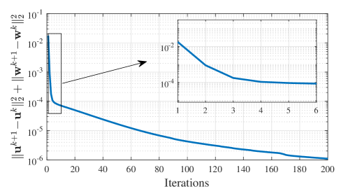
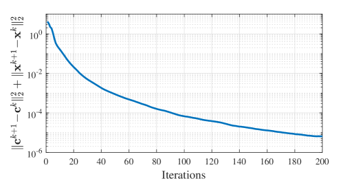
Figureย 3 shows the convergence curves of the proposed ADMM-Direct and ADMM-Relax algorithms. In Figureย 3(a), the residual error of ADMM-Direct is defined as โ€–๐œk+1โˆ’๐œkโ€–22+โ€–๐ฑk+1โˆ’๐ฑkโ€–22superscriptsubscriptnormsuperscript๐œ๐‘˜1superscript๐œ๐‘˜22superscriptsubscriptnormsuperscript๐ฑ๐‘˜1superscript๐ฑ๐‘˜22\|\mathbf{c}^{k+1}-\mathbf{c}^{k}\|_{2}^{2}+\|\mathbf{x}^{k+1}-\mathbf{x}^{k}\|_{2}^{2}, and in Figureย 3(b), the residual error of ADMM-Relax is defined as โ€–๐ฎk+1โˆ’๐ฎkโ€–22+โ€–๐ฐk+1โˆ’๐ฐkโ€–22superscriptsubscriptnormsuperscript๐ฎ๐‘˜1superscript๐ฎ๐‘˜22superscriptsubscriptnormsuperscript๐ฐ๐‘˜1superscript๐ฐ๐‘˜22\|\mathbf{u}^{k+1}-\mathbf{u}^{k}\|_{2}^{2}+\|\mathbf{w}^{k+1}-\mathbf{w}^{k}\|_{2}^{2}. From the curves, we can see that both of the ADMMs can converge after a few iterations. Here, we should note that we do not give the exact proof of the convergence for the ADMM-Direct algorithm. However, we observe that ADMM-Direct can converge from Figureย 3(a). From Figureย 3(b), we can see that the residual error decreases quickly in the first several iterations and after 5 iterations, the convergence curve is relatively flat.
Refer to caption

(a) ADMM-Direct

Refer to caption

(b) ADMM-Relax

Figure 3: The convergence performance of ADMM-Direct and ADMM-Relax with 16-QAM modulation.
Refer to caption
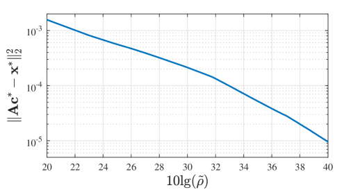
Figure 4: The relationship between โ€–๐€๐œโˆ—โˆ’๐ฑโˆ—โ€–22subscriptsuperscriptnormsuperscript๐€๐œsuperscript๐ฑ22\|\mathbf{Ac}^{*}-\mathbf{x}^{*}\|^{2}_{2} and ฯ~~๐œŒ\tilde{\rho}.

To further illustrate the third part of Theorem 2, which indicates that if (๐œ1,๐ฑ1)superscript๐œ1superscript๐ฑ1(\mathbf{c}^{1},\mathbf{x}^{1}) lies in the feasible region of the model (3), (๐œโˆ—,๐ฑโˆ—)superscript๐œsuperscript๐ฑ(\mathbf{c}^{*},\mathbf{x}^{*}) approaches some KKT point of the model (3) as ฯ~~๐œŒ\tilde{\rho} increases, we plot the curve of the relationship between โ€–๐€๐œโˆ—โˆ’๐ฑโˆ—โ€–22subscriptsuperscriptnormsuperscript๐€๐œsuperscript๐ฑ22\|\mathbf{Ac}^{*}-\mathbf{x}^{*}\|^{2}_{2} and ฯ~~๐œŒ\tilde{\rho} in Figureย 4. In this figure, (๐œโˆ—,๐ฑโˆ—)superscript๐œsuperscript๐ฑ(\mathbf{c}^{*},\mathbf{x}^{*}) is the optimal solution of the model (21). Moreover, we use โ€–๐€๐œโˆ—โˆ’๐ฑโˆ—โ€–22subscriptsuperscriptnormsuperscript๐€๐œsuperscript๐ฑ22\|\mathbf{Ac}^{*}-\mathbf{x}^{*}\|^{2}_{2} to measure whether (๐œโˆ—,๐ฑโˆ—)superscript๐œsuperscript๐ฑ(\mathbf{c}^{*},\mathbf{x}^{*}) approaches some KKT point of the model (3), because if โ€–๐€๐œโˆ—โˆ’๐ฑโˆ—โ€–22subscriptsuperscriptnormsuperscript๐€๐œsuperscript๐ฑ22\|\mathbf{Ac}^{*}-\mathbf{x}^{*}\|^{2}_{2} approaches zero, (๐œโˆ—,๐ฑโˆ—)superscript๐œsuperscript๐ฑ(\mathbf{c}^{*},\mathbf{x}^{*}) approaches some KKT point of the model (3) as Appendix D shows. From the curve, we can see that, โ€–๐€๐œโˆ—โˆ’๐ฑโˆ—โ€–22subscriptsuperscriptnormsuperscript๐€๐œsuperscript๐ฑ22\|\mathbf{Ac}^{*}-\mathbf{x}^{*}\|^{2}_{2} approaches zero as ฯ~~๐œŒ\tilde{\rho} increases as we expected. That is, (๐œโˆ—,๐ฑโˆ—)superscript๐œsuperscript๐ฑ(\mathbf{c}^{*},\mathbf{x}^{*}) approaches some KKT point of (3).

TABLE II: Comparison of EVMs (dB) at different ฮฒ๐›ฝ\beta (Modulation: 16-QAM; PAPR constraint: 4dB)
ฮฒ๐›ฝ\beta EVM
ADMM-Direct ADMM-Relax
0 -16.58dB -16.36dB
0.15 -27.33dB -27.51dB
0.3 -32.96dB -32.89dB

In Table II, we show that the impact of the different values of ฮฒ๐›ฝ\beta on signal distortion introduced to data carriers of OFDM signals. Here, we use averaged error vector magnitude (EVM) to evaluate distortion, which is defined by

EVMยฏ=1Kโ€‹โˆ‘i=1Kโ€–๐’Dโ€‹(๐œโˆ’๐œo)โ€–22โ€–๐œoโ€–22,ยฏEVM1๐พsuperscriptsubscript๐‘–1๐พsubscriptsuperscriptnormsubscript๐’D๐œsubscript๐œo22subscriptsuperscriptnormsubscript๐œo22\overline{\rm EVM}=\sqrt{\frac{1}{K}\displaystyle\sum_{i=1}^{K}\frac{\|\mathbf{S}_{\rm D}(\mathbf{c}-\mathbf{c}_{\rm o})\|^{2}_{2}}{\|\mathbf{c}_{\rm o}\|^{2}_{2}}},

where K๐พK is set 5000 in the simulations. From Table II, we can see clearly that the signal distortion decreases almost 10dB when we increase ฮฒ๐›ฝ\beta from 0 to 0.15. However, when we further increase ฮฒ๐›ฝ\beta from 0.15 to 0.3, the corresponding EVM values, i.e., introduced distortions, only decrease about 5.5dB. Checking the optimized free carriers, we find that the power overheads of some OFDM symbols in the latter are less than the pre-set upper-bound 0.3. It means that the constraint 3(c) becomes inactive for these kinds of OFDM symbols and their optimizers locate inside the defined feasible region. The fact indicates that increasing ฮฒ๐›ฝ\beta can decrease averaged signal distortion of the optimized OFDM symbols efficiently. However, for a larger ฮฒ๐›ฝ\beta, its influence becomes weaker.

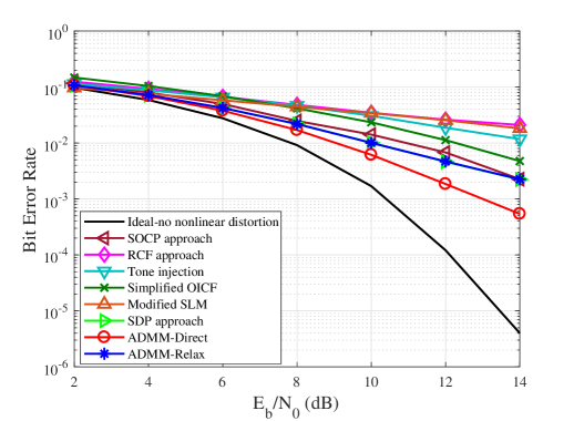
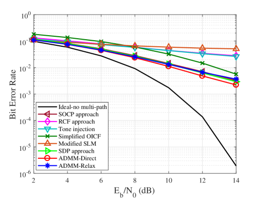
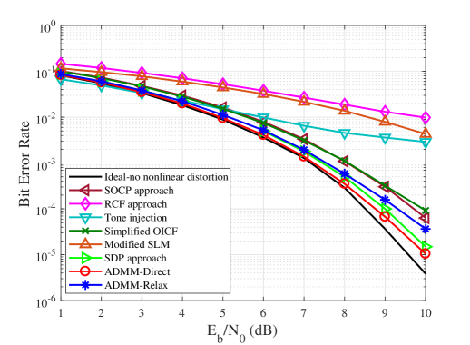
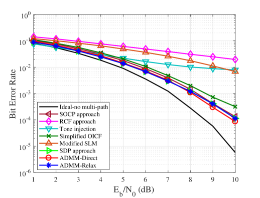
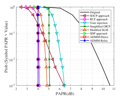
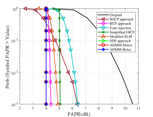
Figureย 5 and Figureย 6 plot PAPR complementary cumulative distribution functions (CCDFs), bit error rate (BER) performance of the original and processed OFDM signals after the solid state PA (SSPA) with smoothing factor 3 (modeled in [3]) and through AWGN channel, and BER performance of OFDM signals after SSPA and through multi-path channel. Data carrier modulations are assumed to be 16-QAM or QPSK. CCDF denotes the probability that the PAPR of the OFDM symbols exceeds some given threshold T๐‘‡T, i.e., CCDFโ€‹(T)=Probโ€‹(PAPR>T)CCDF๐‘‡ProbPAPR๐‘‡{\rm CCDF}({T})={\rm Prob}({\rm PAPR}>{T}). The simulation results of ADMMs are obtained through 5 iterations.
Refer to caption

(a) PAPR reduction performance

Refer to caption

(b) BER performance (after SSPA)

Refer to caption

(b) BER performance (through multi-path channel)

Figure 5: The performance of various systems with 16-QAM modulation(5 iterations for ADMMs, 10 iterations for RCF).

In Figureย 5(a), the word โ€œOriginalโ€ means no distortion is introduced. From the figure, we can see that the proposed ADMMs, RCF, OICF, and SDP, have cut-off CCDF curves. However, the CCDF curves of ADMMs and SDP locate on the left side of the othersโ€™. It means that the former three approaches have better PAPR reduction performance. Moreover, CCDF curves of SOCP, modified SLM and tone injection are slow-down. It means that some of their optimized OFDM symbols still have larger PAPR values. In practice, these kinds of signals would suffer from severe nonlinear distortion of the PA, which can worse BER performance of the OFDM signals. Figureย 5(b) shows the BER curves of the optimized OFDM symbols after SSPA. The input power back-off of the working-point away from saturation region is set as 4.1dB. From it, we can see that BER curves of ADMMs and SDP are closest to the idealโ€™s. Here, the word โ€œidealโ€ means no distortion is introduced in the OFDM symbols. Figureย 6 plots the PAPR-reduction performance and BER performance of the original OFDM signals and the processed OFDM signals with QPSK data carrier modulation. Similar to the performance with 16-QAM modulation, ADMM-Direct and ADMM-Relax still have cut-off PAPR reduction performance. Meanwhile, from Figureย 6(b), we can see that the ADMM-Direct and ADMM-Relax have pretty good BER performance. Here, the input power back-off is also set as 4.1dB. Furthermore, Figureย 5(c) and 6(c) plot the BER curves of the optimized OFDM symbols after SSPA and multi-path channel. Here, four paths are considered and in each path delay/fading parameters are (0,1)01(0,1) (direct path), (190,0.2)1900.2(190,0.2), (300,0.07)3000.07(300,0.07), and (400,0.05)4000.05(400,0.05) respectively. From the figures, we can see that, in comparison with AWGN channel case, BER performance of all PAPR reduction methods becomes worse when multi-path effects are considered. However, ADMM-Direct/-Relax approaches are still better than state-of-the-art approaches. At last, from Figure 5 and 6, we see that SDP approach has similar PAPR reduction performance and BER performance to our proposed ADMM approaches. However, we should note that the computational complexity of SDP is prohibitive in practice, which is roughly ๐’ชโ€‹(โ„“3โ€‹N3)๐’ชsuperscriptโ„“3superscript๐‘3\mathcal{O}(\ell^{3}N^{3}) in each iteration. In comparison, the computational complexity of our ADMMs is roughly ๐’ชโ€‹(โ„“โ€‹Nโ€‹log2โก(โ„“โ€‹N))๐’ชโ„“๐‘subscript2โ„“๐‘\mathcal{O}(\ell N\log_{2}(\ell N)) in each iteration, which is much cheaper than SDP.
Refer to caption

(a) PAPR reduction performance

Refer to caption

(b) BER performance (after SSPA)

Refer to caption

(b) BER performance (through multi-path channel)

Figure 6: The performance of various systems with QPSK modulation(5 iterations for ADMMs, 10 iterations for RCF).

The out-of-band radiation performance is shown in Figureย 7. On the one hand, we can see from the curves that SDP, ADMM-Direct/-Relax and RCF have lower out-of-band emission (OOBE). On the other hand, we can also observe that tone injection and modified SLM have higher OOBE. The reason that OOBE performance of the proposed ADMM-Direct/-Relax approaches and SDP appraoch is better because all of them have cut-off CCDF curves, which means that their processed OFDM symbols have quasi-constant PAPR values. It is well known that OOBE is mainly caused by nonlinear distortion of the OFDM signals. In the simulations, since the input power back-off of the working-point is set as 4.1dB and the PAPR of OFDM symbols optimized by ADMM-Direct/-Relax are almost 4dB (quasi-constant), it means that most of the signals are amplified in the linear region of the PA. So, there is only very small nonlinear distortion (caused by nonlinear PA) introduced into the OFDM symbols. Accordingly, it is reasonable that their OOBEs are low.
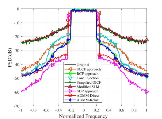
Refer to caption
Figure 7: Out-of-band radiation performance with 16-QAM modulation.

VI Conclusion

This paper proposes two low-complexity iteration optimization methods named ADMM-Direct and ADMM-Relax, to reduce PAPR values of the OFDM signals. Both of their computational complexities in each iteration are similar to the classical RCF method and the desired OFDM symbols can be obtained just after a few iterations; meanwhile, they have quasi-constant PAPR values and optimized signal distortion. Moreover, the resulting solution of ADMM-Direct is guaranteed to be some KKT point of the established model when the iteration algorithm converges. We also prove that ADMM-Relax is convergent and can approach arbitrarily close to some KKT point of the model if proper algorithm parameters are chosen. In comparison with existing algorithms, the proposed ADMM algorithms outperform the existing approaches not only in the simulation results but also in strong theoretically guaranteed performance. In the end, we should mention that high PAPR problem is still an issue in the systems of multiple-input multiple-output (MIMO) and non-orthogonal multiple access (NOMA) [30] when multi-carriers techniques are applied. Designing low-complexity, but theoretically guaranteed, ADMM-like optimization algorithm could be an interesting research topic in the future.

Appendix A Proof of equivalence between models (15) and (16)

The equivalence between the models (15) and (16) is in the sense that the global optimal solution of the latter model is always attained when โ€œ=โ€ holds in (16c). We prove this fact by contradiction. To be clear, we suppose some feasible point ๐ณ~~๐ณ\tilde{\mathbf{z}} satisfies โ€–๐ณ~โ€–22<1superscriptsubscriptnorm~๐ณ221\|\tilde{\mathbf{z}}\|_{2}^{2}<1 and the constraint (16b). Notice that the constant modulus ๐ณ~~๐ณ\tilde{\mathbf{z}} is in the feasible region since ฮฑ๐›ผ\alpha is greater than 1. Therefore, we can always find a vector โ–ณ๐ณ~โ–ณ~๐ณ\bigtriangleup\tilde{\mathbf{z}}, whose phase vector is equal to that of vector ๐›ksuperscript๐›๐‘˜\mathbf{b}^{k}, which can let ๐ณ~+โ–ณ๐ณ~\tilde{\mathbf{z}}+\bigtriangleup\tilde{\mathbf{z}} satisfy the constraints (16b) and (16c). It is obvious that the new vector corresponds to a larger objective value, which means that ๐ณ~~๐ณ\tilde{\mathbf{z}} is not the global optimal solution of the model (16). So, we can conclude that the maximizer in model (16) should always satisfy (16c) when โ€œ=โ€ holds.

Appendix B Proof of Theorem 1

To be clear, we let Lโ€‹(๐œ,๐ฑ,ฮณ,ฮผ,๐ฒ)๐ฟ๐œ๐ฑ๐›พ๐œ‡๐ฒL(\mathbf{c},\mathbf{x},\gamma,\mu,\mathbf{y}), L๐œโ€‹(๐œ,๐ฒ,ฮผ)superscript๐ฟ๐œ๐œ๐ฒ๐œ‡L^{\mathbf{c}}(\mathbf{c},\mathbf{y},\mu), and L๐ฑโ€‹(๐ฑ,๐ฒ,ฮณ)superscript๐ฟ๐ฑ๐ฑ๐ฒ๐›พL^{\mathbf{x}}(\mathbf{x},\mathbf{y},\gamma) be the Lagrangian functions of the model (3), (4a), and (4b) respectively. ฮผ๐œ‡\mu and ฮณ๐›พ\gamma are the Lagrangian multipliers corresponding to the constraints (3c) and (3b) respectively. We also let ฮผโˆ—superscript๐œ‡\mu^{*} and ฮณโˆ—superscript๐›พ\gamma^{*} be the corresponding optimal Lagrangian multipliers when ADMM-Direct algorithm is convergent. To show (๐œโˆ—,๐ฑโˆ—)superscript๐œsuperscript๐ฑ(\mathbf{c}^{*},\mathbf{x}^{*}) is a KKT point, we should prove that it, combining (๐ฒโˆ—superscript๐ฒ\mathbf{y}^{*}, ฮผโˆ—superscript๐œ‡\mu^{*}, ฮณโˆ—superscript๐›พ\gamma^{*} ), should satisfy the conditions of the primal feasibility (25a), the dual feasibility (25b) and the complementary slackness (25c), and is also a stationary point of the Lagrangian function Lโ€‹(๐œ,๐ฑ,ฮณ,ฮผ,๐ฒ)๐ฟ๐œ๐ฑ๐›พ๐œ‡๐ฒL(\mathbf{c},\mathbf{x},\gamma,\mu,\mathbf{y}), i.e.,

๐œโˆ—โˆˆ๐’ž,๐ฑโˆ—โˆˆ๐’ณ,formulae-sequencesuperscript๐œ๐’žsuperscript๐ฑ๐’ณ\displaystyle\mathbf{c^{*}\in\mathcal{C}},\ \ \mathbf{x^{*}\in\mathcal{X}}, (25a)
ฮผโˆ—โ‰ฅ0,superscript๐œ‡0\displaystyle\mu^{*}\geq 0, (25b)
ฮผโˆ—โ€‹(โ€–๐’Fโ€‹๐œโˆ—โ€–22โˆ’ฮฒโ€‹โ€–๐’Dโ€‹๐œโˆ—โ€–22)=0,superscript๐œ‡superscriptsubscriptnormsubscript๐’Fsuperscript๐œ22๐›ฝsuperscriptsubscriptnormsubscript๐’Dsuperscript๐œ220\displaystyle\mu^{*}(\|\mathbf{S}_{\rm F}\mathbf{c}^{*}\|_{2}^{2}-\beta\|\mathbf{S}_{\rm D}\mathbf{c}^{*}\|_{2}^{2})=0, (25c)
โˆ‡๐œLโ€‹(๐œโˆ—,๐ฑโˆ—,ฮณโˆ—,ฮผโˆ—,๐ฒโˆ—)=0,subscriptโˆ‡๐œ๐ฟsuperscript๐œsuperscript๐ฑsuperscript๐›พsuperscript๐œ‡superscript๐ฒ0\displaystyle\nabla_{\mathbf{c}}{L}(\mathbf{c}^{*},\mathbf{x}^{*},\gamma^{*},\mu^{*},\mathbf{y}^{*})=0, (25d)
โˆ‡๐ฑLโ€‹(๐œโˆ—,๐ฑโˆ—,ฮณโˆ—,ฮผโˆ—,๐ฒโˆ—)=0,subscriptโˆ‡๐ฑ๐ฟsuperscript๐œsuperscript๐ฑsuperscript๐›พsuperscript๐œ‡superscript๐ฒ0\displaystyle\nabla_{\mathbf{x}}L(\mathbf{c}^{*},\mathbf{x}^{*},\gamma^{*},\mu^{*},\mathbf{y}^{*})=0, (25e)

where ๐’ณ๐’ณ\mathcal{X} and ๐’ž๐’ž\mathcal{C} denote the constraints (3b) and (3c) respectively.

Since in every ADMM-Direct iteration, ๐œk+1superscript๐œ๐‘˜1\mathbf{c}^{k+1} and ๐ฑk+1superscript๐ฑ๐‘˜1\mathbf{x}^{k+1} are located in the feasible region, we can see that the primal feasibility condition (25a) is satisfied. Since ฮผkโฃโˆ—superscript๐œ‡๐‘˜\mu^{k*} is guaranteed to be greater than zero (see (12)) in every iteration, it means that ฮผโˆ—superscript๐œ‡\mu^{*} is also greater than zero. Moreover, checking (12) again, we see that the value of ฮผkโฃโˆ—,โˆ€k,superscript๐œ‡๐‘˜for-all๐‘˜\mu^{k*},\ \forall k, is nonzero or zero corresponding to the constraint (3c), which is active or inactive respectively. It means that ฮผโˆ—superscript๐œ‡\mu^{*} satisfies the condition of complementary slackness.

Now, let us consider (25d) and (25e). Since ๐œk+1superscript๐œ๐‘˜1\mathbf{c}^{k+1} and ๐ฑk+1superscript๐ฑ๐‘˜1{\mathbf{x}^{k+1}} are the minimizers of the problems (4a) and (4b) in the k๐‘˜kth iteration respectively, they should satisfy

โˆ‡๐œL๐œโ€‹(๐œk+1,๐ฒk,ฮผkโฃโˆ—)+ฯโ€‹๐€Hโ€‹(๐€๐œk+1โˆ’๐ฑk)=0,โˆ‡๐ฑL๐ฑโ€‹(๐ฑk+1,๐ฒk,ฮณkโฃโˆ—)โˆ’ฯโ€‹(๐€๐œk+1โˆ’๐ฑk+1)=0.formulae-sequencesubscriptโˆ‡๐œsuperscript๐ฟ๐œsuperscript๐œ๐‘˜1superscript๐ฒ๐‘˜superscript๐œ‡๐‘˜๐œŒsuperscript๐€๐ปsuperscript๐€๐œ๐‘˜1superscript๐ฑ๐‘˜0subscriptโˆ‡๐ฑsuperscript๐ฟ๐ฑsuperscript๐ฑ๐‘˜1superscript๐ฒ๐‘˜superscript๐›พ๐‘˜๐œŒsuperscript๐€๐œ๐‘˜1superscript๐ฑ๐‘˜10\begin{split}&\nabla_{\mathbf{c}}{L}^{\mathbf{c}}(\mathbf{c}^{k+1},\mathbf{y}^{k},\mu^{k*})+\rho\mathbf{A}^{H}(\mathbf{Ac}^{k+1}-\mathbf{x}^{k})=0,\\ &\nabla_{\mathbf{x}}{L}^{\mathbf{x}}(\mathbf{x}^{k+1},\mathbf{y}^{k},\gamma^{k*})-\rho(\mathbf{Ac}^{k+1}-\mathbf{x}^{k+1})=0.\end{split} (26)

Since limkโ†’+โˆžโ€‹(๐œk,๐ฑk,๐ฒk)=(๐œโˆ—,๐ฑโˆ—,๐ฒโˆ—)โ†’๐‘˜superscript๐œ๐‘˜superscript๐ฑ๐‘˜superscript๐ฒ๐‘˜superscript๐œsuperscript๐ฑsuperscript๐ฒ\underset{k\rightarrow+\infty}{\lim}(\mathbf{c}^{k},\mathbf{x}^{k},\mathbf{y}^{k})=(\mathbf{c}^{*},\mathbf{x}^{*},\mathbf{y}^{*}) and ๐ฒk+1=๐ฒk+ฯโ€‹(๐€๐œk+1โˆ’๐ฑk+1)superscript๐ฒ๐‘˜1superscript๐ฒ๐‘˜๐œŒsuperscript๐€๐œ๐‘˜1superscript๐ฑ๐‘˜1\mathbf{y}^{k+1}=\mathbf{y}^{k}+\rho(\mathbf{Ac}^{k+1}-\mathbf{x}^{k+1}), we can drop the second terms in (26) as kโ†’+โˆžโ†’๐‘˜k\rightarrow+\infty and obtain

โˆ‡๐œL๐œโ€‹(๐œโˆ—,๐ฒโˆ—,ฮผโˆ—)=0,โˆ‡๐ฑL๐ฑโ€‹(๐ฑโˆ—,๐ฒโˆ—,ฮณโˆ—)=0.\begin{split}&\nabla_{\mathbf{c}}{L}^{\mathbf{c}}(\mathbf{c}^{*},\mathbf{y}^{*},\mu^{*})=0,\ \ \nabla_{\mathbf{x}}L^{\mathbf{x}}(\mathbf{x}^{*},\mathbf{y}^{*},\gamma^{*})=0.\end{split} (27)

Since there are โˆ‡๐œL๐œโ€‹(๐œโˆ—,๐ฒโˆ—,ฮผโˆ—)=โˆ‡๐œLโ€‹(๐œโˆ—,๐ฑโˆ—,ฮณโˆ—,ฮผโˆ—,๐ฒโˆ—)subscriptโˆ‡๐œsuperscript๐ฟ๐œsuperscript๐œsuperscript๐ฒsuperscript๐œ‡subscriptโˆ‡๐œ๐ฟsuperscript๐œsuperscript๐ฑsuperscript๐›พsuperscript๐œ‡superscript๐ฒ\nabla_{\mathbf{c}}{L}^{\mathbf{c}}(\mathbf{c}^{*},\mathbf{y}^{*},\mu^{*})=\nabla_{\mathbf{c}}{L}(\mathbf{c}^{*},\mathbf{x}^{*},\gamma^{*},\mu^{*},\mathbf{y}^{*}) and โˆ‡๐ฑL๐ฑโ€‹(๐ฑโˆ—,๐ฒโˆ—,ฮณโˆ—)=โˆ‡๐ฑLโ€‹(๐œโˆ—,๐ฑโˆ—,ฮณโˆ—,ฮผโˆ—,๐ฒโˆ—)subscriptโˆ‡๐ฑsuperscript๐ฟ๐ฑsuperscript๐ฑsuperscript๐ฒsuperscript๐›พsubscriptโˆ‡๐ฑ๐ฟsuperscript๐œsuperscript๐ฑsuperscript๐›พsuperscript๐œ‡superscript๐ฒ\nabla_{\mathbf{x}}{L}^{\mathbf{x}}(\mathbf{x}^{*},\mathbf{y}^{*},\gamma^{*})=\nabla_{\mathbf{x}}{L}(\mathbf{c}^{*},\mathbf{x}^{*},\gamma^{*},\mu^{*},\mathbf{y}^{*}), we can see that (๐œโˆ—,๐ฑโˆ—,๐ฒโˆ—)superscript๐œsuperscript๐ฑsuperscript๐ฒ(\mathbf{c}^{*},\mathbf{x}^{*},\mathbf{y}^{*}) should satisfy (25d) and (25e), i.e., it is a stationary point of the Lagrangian function Lโ€‹(๐œ,๐ฑ,ฮณ,ฮผ,๐ฒ)๐ฟ๐œ๐ฑ๐›พ๐œ‡๐ฒL(\mathbf{c},\mathbf{x},\gamma,\mu,\mathbf{y}). This concludes the proof of Theorem 1.

Appendix C Solving the optimization subproblems (23a)-(23c)

C-A Solving the Subproblem (23a)

Based on the augmented Lagrangian function (22), the problem (23a) is equivalent to

min๐œโˆˆโ„‚N12โ€‹โ€–๐’Dโ€‹(๐œโˆ’๐œo)โ€–22+ฯ2โ€‹โ€–๐€๐œโˆ’๐ฎk+๐ฒ1kฯโ€–22,๐œsuperscriptโ„‚๐‘min12superscriptsubscriptnormsubscript๐’D๐œsubscript๐œo22๐œŒ2superscriptsubscriptnorm๐€๐œsuperscript๐ฎksuperscriptsubscript๐ฒ1k๐œŒ22\displaystyle\underset{\displaystyle\mathbf{c}\in\mathbb{C}^{N}}{\rm min}\hskip 14.22636pt\frac{1}{2}\|\mathbf{S}_{\rm D}(\mathbf{c}-\mathbf{c}_{\rm o})\|_{2}^{2}+\frac{\rho}{2}\|\mathbf{Ac}-\mathbf{u}^{k}+\frac{\mathbf{y}_{1}^{k}}{\rho}\|_{2}^{2}, (28a)
subjectโ€‹toโ€‹โ€–๐’Fโ€‹๐œโ€–22โˆ’ฮฒโ€‹โ€–๐’Dโ€‹๐œโ€–22โ‰ค0.subjecttosuperscriptsubscriptnormsubscript๐’F๐œ22๐›ฝsuperscriptsubscriptnormsubscript๐’D๐œ220\displaystyle{\rm subject\ to}\hskip 7.53996pt\|\mathbf{S}_{\rm F}\mathbf{c}\|_{2}^{2}-\beta\|\mathbf{S}_{\rm D}\mathbf{c}\|_{2}^{2}\leq 0. (28b)

Its Lagrangian function can be written as

Lโ€‹(๐œ,ฮผk)=12โ€‹โ€–๐’Dโ€‹(๐œโˆ’๐œo)โ€–22+ฯ2โ€‹โ€–๐€๐œโˆ’๐ฎk+๐ฒ1kฯโ€–22+ฮผkโ€‹(โ€–๐’Fโ€‹๐œโ€–22โˆ’ฮฒโ€‹โ€–๐’Dโ€‹๐œโ€–22),๐ฟ๐œsuperscript๐œ‡๐‘˜12superscriptsubscriptdelimited-โˆฅโˆฅsubscript๐’D๐œsubscript๐œo22๐œŒ2superscriptsubscriptdelimited-โˆฅโˆฅ๐€๐œsuperscript๐ฎ๐‘˜superscriptsubscript๐ฒ1๐‘˜๐œŒ22superscript๐œ‡๐‘˜superscriptsubscriptdelimited-โˆฅโˆฅsubscript๐’F๐œ22๐›ฝsuperscriptsubscriptdelimited-โˆฅโˆฅsubscript๐’D๐œ22\begin{split}L(\mathbf{c},\mu^{k})&=\frac{1}{2}\|\mathbf{S}_{\rm D}(\mathbf{c}-\mathbf{c}_{\rm o})\|_{2}^{2}+\frac{\rho}{2}\|\mathbf{Ac}-\mathbf{u}^{k}+\frac{\mathbf{y}_{1}^{k}}{\rho}\|_{2}^{2}\\ &\hskip 14.22636pt+\mu^{k}\big{(}\|\mathbf{S}_{\rm F}\mathbf{c}\|_{2}^{2}-\beta\|\mathbf{S}_{\rm D}\mathbf{c}\|_{2}^{2}\big{)},\end{split} (29)

where the Lagrangian multiplier is ฮผkโ‰ฅ0superscript๐œ‡๐‘˜0\mu^{k}\geq 0. Since the global optimal solution ๐œk+1superscript๐œ๐‘˜1\mathbf{c}^{k+1}, combining the optimal Lagrangian multiplier ฮผkโฃโˆ—superscript๐œ‡๐‘˜\mu^{k*} should satisfy โˆ‡๐œLโ€‹(๐œk+1,ฮผkโฃโˆ—)=0subscriptโˆ‡๐œ๐ฟsuperscript๐œ๐‘˜1superscript๐œ‡๐‘˜0\displaystyle\nabla_{\mathbf{c}}L(\mathbf{c}^{k+1},\mu^{k*})=0, we can get

๐œk+1=(๐’D+ฯโ„“โ€‹Nโ€‹๐ˆ+2โ€‹ฮผkโฃโˆ—โ€‹(๐’Fโˆ’ฮฒโ€‹๐’D))โ€ โ€‹๐ฏk,superscript๐œ๐‘˜1superscriptsubscript๐’D๐œŒโ„“๐‘๐ˆ2superscript๐œ‡๐‘˜subscript๐’F๐›ฝsubscript๐’Dโ€ superscript๐ฏ๐‘˜\mathbf{c}^{k+1}=\big{(}\mathbf{S}_{\rm D}+\frac{\rho}{\ell N}\mathbf{I}+2\mu^{k*}(\mathbf{S}_{\rm F}-\beta\mathbf{S}_{\rm D})\big{)}^{\dagger}\mathbf{v}^{k}, (30)

where ๐ฏk=๐œo+ฯโ€‹๐€Hโ€‹(๐ฎkโˆ’๐ฒ1kฯ)superscript๐ฏ๐‘˜subscript๐œo๐œŒsuperscript๐€๐ปsuperscript๐ฎ๐‘˜superscriptsubscript๐ฒ1๐‘˜๐œŒ\displaystyle\mathbf{v}^{k}=\mathbf{c}_{\rm o}+\rho\mathbf{A}^{H}(\mathbf{u}^{k}-\frac{\mathbf{y}_{1}^{k}}{\rho}).

Moreover, when the constraint (28b) is inactive, ๐œk+1superscript๐œ๐‘˜1\mathbf{c}^{k+1} is located inside the feasible region ๐’ž๐’ž\mathcal{C}. It means that ฮผkโฃโˆ—=0superscript๐œ‡๐‘˜0\mu^{k*}=0. Otherwise, if the constraint (28b) is active, it means that ๐œk+1superscript๐œ๐‘˜1\mathbf{c}^{k+1} and the optimal Lagrangian multiplier ฮผkโฃโˆ—superscript๐œ‡๐‘˜\mu^{k*} should satisfy the constraint (28b) when โ€œ=โ€ holds. Plugging (30) into โ€–๐’Fโ€‹๐œk+1โ€–2subscriptnormsubscript๐’Fsuperscript๐œ๐‘˜12\|\mathbf{S}_{\rm F}\mathbf{c}^{k+1}\|_{2} and โ€–๐’Dโ€‹๐œk+1โ€–2subscriptnormsubscript๐’Dsuperscript๐œ๐‘˜12\|\mathbf{S}_{\rm D}\mathbf{c}^{k+1}\|_{2}, we can obtain

โ€–๐’Fโ€‹๐œk+1โ€–2=โ€–๐’Fโ€‹๐ฏkโ€–2ฯโ„“โ€‹N+2โ€‹ฮผkโฃโˆ—,โ€–๐’Dโ€‹๐œk+1โ€–2=โ€–๐’Dโ€‹๐ฏkโ€–21+ฯโ„“โ€‹Nโˆ’2โ€‹ฮผkโฃโˆ—โ€‹ฮฒ.formulae-sequencesubscriptdelimited-โˆฅโˆฅsubscript๐’Fsuperscript๐œ๐‘˜12subscriptnormsubscript๐’Fsuperscript๐ฏ๐‘˜2๐œŒโ„“๐‘2superscript๐œ‡๐‘˜subscriptdelimited-โˆฅโˆฅsubscript๐’Dsuperscript๐œ๐‘˜12subscriptnormsubscript๐’Dsuperscript๐ฏ๐‘˜21๐œŒโ„“๐‘2superscript๐œ‡๐‘˜๐›ฝ\begin{split}&\|\mathbf{S}_{\rm F}\mathbf{c}^{k+1}\|_{2}=\frac{\|\mathbf{S}_{\rm F}\mathbf{v}^{k}\|_{2}}{\frac{\rho}{\ell N}+2\mu^{k*}},\\ &\|\mathbf{S}_{\rm D}\mathbf{c}^{k+1}\|_{2}=\frac{\|\mathbf{S}_{\rm D}\mathbf{v}^{k}\|_{2}}{1+\frac{\rho}{\ell N}-2\mu^{k*}\beta}.\end{split} (31)

Then, we can solve ฮผkโฃโˆ—superscript๐œ‡๐‘˜\mu^{k*} as (32) when โ€–๐’Fโ€‹๐œk+1โ€–22=ฮฒโ€‹โ€–๐’Dโ€‹๐œk+1โ€–22superscriptsubscriptnormsubscript๐’Fsuperscript๐œ๐‘˜122๐›ฝsuperscriptsubscriptnormsubscript๐’Dsuperscript๐œ๐‘˜122\|\mathbf{S}_{\rm F}\mathbf{c}^{k+1}\|_{2}^{2}=\beta\|\mathbf{S}_{\rm D}\mathbf{c}^{k+1}\|_{2}^{2}.

ฮผkโฃโˆ—=(1+ฯโ„“โ€‹N)โ€‹โ€–๐’Fโ€‹๐ฏkโ€–2โˆ’ฮฒโ€‹ฯโ„“โ€‹Nโ€‹โ€–๐’Dโ€‹๐ฏkโ€–22โ€‹(ฮฒโ€‹โ€–๐’Fโ€‹๐ฏkโ€–2+ฮฒโ€‹โ€–๐’Dโ€‹๐ฏkโ€–2).superscript๐œ‡๐‘˜1๐œŒโ„“๐‘subscriptnormsubscript๐’Fsuperscript๐ฏ๐‘˜2๐›ฝ๐œŒโ„“๐‘subscriptnormsubscript๐’Dsuperscript๐ฏ๐‘˜22๐›ฝsubscriptnormsubscript๐’Fsuperscript๐ฏ๐‘˜2๐›ฝsubscriptnormsubscript๐’Dsuperscript๐ฏ๐‘˜2\mu^{k*}=\frac{\big{(}1+\frac{\rho}{\ell N}\big{)}\|\mathbf{S}_{\rm F}\mathbf{v}^{k}\|_{2}-\sqrt{\beta}\frac{\rho}{\ell N}\|\mathbf{S}_{\rm D}\mathbf{v}^{k}\|_{2}}{2(\beta\|\mathbf{S}_{\rm F}\mathbf{v}^{k}\|_{2}+\sqrt{\beta}\|\mathbf{S}_{\rm D}\mathbf{v}^{k}\|_{2})}. (32)

Furthermore, observing (32), we see that the computed result for ฮผkโฃโˆ—superscript๐œ‡๐‘˜\mu^{k*} could be negative. However, the Lagrangian multiplier theory guarantees that ฮผkโฃโˆ—superscript๐œ‡๐‘˜\mu^{k*} should always be nonnegative since it is an inequality constraint (28b). This contradiction comes from the assumption that the constraint is active. It means that the constraint is inactive, therefore ฮผkโฃโˆ—superscript๐œ‡๐‘˜\mu^{k*} should be zero. Based on this fact, we compute ฮผkโฃโˆ—superscript๐œ‡๐‘˜\mu^{k*} by

ฮผkโฃโˆ—=maxโก{0,(1+ฯโ„“โ€‹N)โ€‹โ€–๐’Fโ€‹๐ฏkโ€–2โˆ’ฮฒโ€‹ฯโ„“โ€‹Nโ€‹โ€–๐’Dโ€‹๐ฏkโ€–22โ€‹(ฮฒโ€‹โ€–๐’Fโ€‹๐ฏkโ€–2+ฮฒโ€‹โ€–๐’Dโ€‹๐ฏkโ€–2)}.superscript๐œ‡๐‘˜01๐œŒโ„“๐‘subscriptnormsubscript๐’Fsuperscript๐ฏ๐‘˜2๐›ฝ๐œŒโ„“๐‘subscriptnormsubscript๐’Dsuperscript๐ฏ๐‘˜22๐›ฝsubscriptnormsubscript๐’Fsuperscript๐ฏ๐‘˜2๐›ฝsubscriptnormsubscript๐’Dsuperscript๐ฏ๐‘˜2\mu^{k*}\!=\!\max\!\bigg{\{}\!0,\!\frac{\big{(}1\!+\!\frac{\rho}{\ell N}\big{)}\|\mathbf{S}_{\rm F}\mathbf{v}^{k}\|_{2}\!-\!\sqrt{\beta}\frac{\rho}{\ell N}\|\mathbf{S}_{\rm D}\mathbf{v}^{k}\|_{2}}{2(\beta\|\mathbf{S}_{\rm F}\mathbf{v}^{k}\|_{2}+\sqrt{\beta}\|\mathbf{S}_{\rm D}\mathbf{v}^{k}\|_{2})}\bigg{\}}. (33)

C-B Solving the Subproblem (23b)

The problem (23b) can be equivalent to

min๐ฑโˆˆโ„‚โ„“โ€‹Nโ€–๐ฑโˆ’๐ฐk+๐ฒ2kฯโ€–22,๐ฑsuperscriptโ„‚โ„“๐‘minsuperscriptsubscriptnorm๐ฑsuperscript๐ฐksuperscriptsubscript๐ฒ2k๐œŒ22\displaystyle\underset{\displaystyle\mathbf{x}\in\mathbb{C}^{\ell N}}{\rm min}\hskip 14.22636pt\|\mathbf{x}-\mathbf{w}^{k}+\frac{\mathbf{y}_{2}^{k}}{\rho}\|_{2}^{2}, (34a)
subjectโ€‹toโ€–๐ฑโ€–โˆž21โ„“โ€‹Nโ€‹โ€–๐ฑโ€–22=ฮฑ.subjecttosuperscriptsubscriptnorm๐ฑ21โ„“๐‘superscriptsubscriptnorm๐ฑ22๐›ผ\displaystyle{\rm subject\ to}\hskip 14.22636pt\frac{\|\mathbf{x}\|_{\infty}^{2}}{\frac{1}{\ell N}\|\mathbf{x}\|_{2}^{2}}=\alpha. (34b)

Similar to the ADMM-Direct algorithm, we also introduce auxiliary variables t๐‘กt and ๐ณ๐ณ\mathbf{z} to express ๐ฑ๐ฑ\mathbf{x} by ๐ฑ=tโ€‹๐ณ๐ฑ๐‘ก๐ณ\mathbf{x}=t\mathbf{z}, where t>0๐‘ก0t>0 and โ€–๐ณโ€–22=1superscriptsubscriptnorm๐ณ221\|\mathbf{z}\|_{2}^{2}=1. Plugging the auxiliary variables t๐‘กt and ๐ณ๐ณ\mathbf{z} into the problem (34), we can obtain

min๐ณโˆˆโ„‚โ„“โ€‹N,t>0โ€‹t2โˆ’2โ€‹tโ€‹Rโ€‹eโ€‹(๐ณHโ€‹๐›k),formulae-sequence๐ณsuperscriptโ„‚โ„“๐‘๐‘ก0minsuperscriptt22tResuperscript๐ณHsuperscript๐›k\displaystyle\underset{\displaystyle\mathbf{z}\in\mathbb{C}^{\ell N},t>0}{\rm min}\hskip 8.5359ptt^{2}-2t{\rm Re}(\mathbf{z}^{H}\mathbf{b}^{k}), (35a)
subjectโ€‹to|zi|2โ‰คฮฑโ„“โ€‹N,i=1,โ‹ฏ,โ„“โ€‹N,formulae-sequencesubjecttosuperscriptsubscript๐‘ง๐‘–2๐›ผโ„“๐‘๐‘–1โ‹ฏโ„“๐‘\displaystyle\hskip 13.6572pt{\rm subject\ to}\hskip 14.22636pt|z_{i}|^{2}\leq\frac{\alpha}{\ell N},\ \ i=1,\dotsb,\ell N, (35b)
โ€–๐ณโ€–22=1,superscriptsubscriptnorm๐ณ221\displaystyle\hskip 73.97733pt\|\mathbf{z}\|_{2}^{2}=1, (35c)

where ๐›k=๐ฐkโˆ’๐ฒ2kฯ.superscript๐›๐‘˜superscript๐ฐ๐‘˜superscriptsubscript๐ฒ2๐‘˜๐œŒ\displaystyle\mathbf{b}^{k}=\mathbf{w}^{k}-\frac{\mathbf{y}_{2}^{k}}{\rho}.

To solve ๐ณk+1superscript๐ณ๐‘˜1\mathbf{z}^{k+1}, we can drop t๐‘กt from the model (35) and formulate the following equivalent convex optimization model.

max๐ณโˆˆโ„‚โ„“โ€‹NReโ€‹(๐ณHโ€‹๐›k),๐ณsuperscriptโ„‚โ„“๐‘maxResuperscript๐ณHsuperscript๐›k\displaystyle\underset{\displaystyle\mathbf{z}\in\mathbb{C}^{\ell N}}{\rm max}\hskip 17.07182pt{\rm Re}(\mathbf{z}^{H}\mathbf{b}^{k}), (36a)
subjectโ€‹toโ€‹|zi|2โ‰คฮฑโ„“โ€‹N,i=1,โ‹ฏ,โ„“โ€‹N,formulae-sequencesubjecttosuperscriptsubscript๐‘ง๐‘–2๐›ผโ„“๐‘๐‘–1โ‹ฏโ„“๐‘\displaystyle{\rm subject\ to}\hskip 8.5359pt|z_{i}|^{2}\leq\frac{\alpha}{\ell N},\ \ i=1,\dotsb,\ell N, (36b)
โ€–๐ณโ€–22โ‰ค1.superscriptsubscriptnorm๐ณ221\displaystyle\hskip 52.63777pt\|\mathbf{z}\|_{2}^{2}\leq 1. (36c)

By introducing the Lagrangian multiplier ฮณk>0superscript๐›พ๐‘˜0\gamma^{k}>0 for the constraint (36c), we can change the model (36) to

minziโˆˆโ„‚,ฮณk>0โ€‹โˆ‘i=1โ„“โ€‹Nโˆ’Reโ€‹(ziโ€ โ€‹bik)+ฮณkโ€‹(โˆ‘i=1โ„“โ€‹N|zi|2โˆ’1),formulae-sequencesubscript๐‘ง๐‘–โ„‚superscript๐›พ๐‘˜0minsuperscriptsubscripti1โ„“NResuperscriptsubscriptziโ€ superscriptsubscriptbiksuperscript๐›พksuperscriptsubscripti1โ„“Nsuperscriptsubscriptzi21\displaystyle\underset{\displaystyle{z_{i}}\in\mathbb{C},\gamma^{k}>0}{\rm min}\hskip 8.5359pt\displaystyle\sum_{i=1}^{\ell N}-{\rm Re}(z_{i}^{\dagger}b_{i}^{k})+{\gamma}^{k}\big{(}\displaystyle\sum_{i=1}^{\ell N}|z_{i}|^{2}-1\big{)}, (37a)
subjectโ€‹to|zi|โ‰คฮฑโ„“โ€‹N,i=1,โ‹ฏ,โ„“โ€‹N.formulae-sequencesubjecttosubscript๐‘ง๐‘–๐›ผโ„“๐‘๐‘–1โ‹ฏโ„“๐‘\displaystyle\hskip 13.6572pt{\rm subject\ to}\hskip 17.07182pt|z_{i}|\leq\sqrt{\frac{\alpha}{\ell N}},\ \ i=1,\dotsb,\ell N. (37b)

Since both the objective function (37a) and constraint (37b) are treated separately in the variable zisubscript๐‘ง๐‘–z_{i}, solving the model (37) is equivalent to solving the following โ„“โ€‹Nโ„“๐‘\ell N subproblems, which can be performed in parallel.

minziโˆˆโ„‚,ฮณk>0โˆ’Reโ€‹(ziโ€ โ€‹bik)+ฮณkโ€‹|zi|2,formulae-sequencesubscript๐‘ง๐‘–โ„‚superscript๐›พ๐‘˜0minResuperscriptsubscriptziโ€ superscriptsubscriptbiksuperscript๐›พksuperscriptsubscriptzi2\displaystyle\underset{\displaystyle{z_{i}}\in\mathbb{C},\gamma^{k}>0}{\rm min}\hskip 8.5359pt-{\rm Re}(z_{i}^{\dagger}b_{i}^{k})+\gamma^{k}|z_{i}|^{2}, (38a)
subjectโ€‹to|zi|โ‰คฮฑโ„“โ€‹N.subjecttosubscript๐‘ง๐‘–๐›ผโ„“๐‘\displaystyle\hskip 13.6572pt{\rm subject\ to}\hskip 17.07182pt|z_{i}|\leq\sqrt{\frac{\alpha}{\ell N}}. (38b)

Moreover, since only one constraint is involved in (38), its optimal solution can be obtained through (39).

zik+1={bik2โ€‹ฮณk,|bik|2โ€‹ฮณk<ฮฑโ„“โ€‹N,ฮฑโ„“โ€‹Nโ€‹ejโ€‹ฯ•โ€‹(bik),otherwise,superscriptsubscript๐‘ง๐‘–๐‘˜1casessuperscriptsubscript๐‘๐‘–๐‘˜2superscript๐›พ๐‘˜superscriptsubscript๐‘๐‘–๐‘˜2superscript๐›พ๐‘˜๐›ผโ„“๐‘otherwise๐›ผโ„“๐‘superscript๐‘’๐‘—italic-ฯ•superscriptsubscript๐‘๐‘–๐‘˜otherwiseotherwisez_{i}^{k+1}=\begin{cases}\hskip 14.22636pt\displaystyle\frac{b_{i}^{k}}{2\gamma^{k}},\hskip 28.45274pt\frac{|b_{i}^{k}|}{2\gamma^{k}}<\sqrt{\frac{\alpha}{\ell N}},\\ \sqrt{\frac{\alpha}{\ell N}}e^{\displaystyle j\phi(b_{i}^{k})},\ \ {\rm otherwise},\end{cases} (39)

where ฯ•โ€‹(bik)italic-ฯ•superscriptsubscript๐‘๐‘–๐‘˜\phi(b_{i}^{k}) represents the phase of biksuperscriptsubscript๐‘๐‘–๐‘˜b_{i}^{k}. Furthermore, since ๐ณk+1superscript๐ณ๐‘˜1\mathbf{z}^{k+1} should satisfy the constraint โ€–๐ณk+1โ€–22=1superscriptsubscriptnormsuperscript๐ณ๐‘˜1221\|\mathbf{z}^{k+1}\|_{2}^{2}=1, the optimal Lagrangian multiplier ฮณkโฃโˆ—superscript๐›พ๐‘˜\gamma^{k*} can be determined by the binary section searching procedure as shown in Table I. After that, plugging the obtained ๐ณk+1superscript๐ณ๐‘˜1\mathbf{z}^{k+1} into the model (36) and simplifying it as a quadratic problem, we can get tk+1=Reโ€‹(๐ณk+1โ€‹Hโ€‹๐›k)superscript๐‘ก๐‘˜1Resuperscript๐ณ๐‘˜1๐ปsuperscript๐›๐‘˜t^{k+1}={\rm Re}\big{(}\mathbf{z}^{k+1H}\mathbf{b}^{k}\big{)}. At last, plugging ๐ณk+1superscript๐ณ๐‘˜1\mathbf{z}^{k+1} and tk+1superscript๐‘ก๐‘˜1t^{k+1} into ๐ฑ=tโ€‹๐ณ๐ฑ๐‘ก๐ณ\mathbf{x}=t\mathbf{z}, we get the optimal solution ๐ฑk+1superscript๐ฑ๐‘˜1\mathbf{x}^{k+1} of (34).

C-C Solving the Subproblem (23c)

Since the problem (23c) is an unconstrained quadratic problem, its optimal solution (๐ฎk+1,๐ฐk+1)superscript๐ฎ๐‘˜1superscript๐ฐ๐‘˜1(\mathbf{u}^{k+1},\mathbf{w}^{k+1}) should satisfy

โˆ‡๐ฎLฯโ€‹(๐ฑk+1,๐œk+1,๐ฎk+1,๐ฐk+1,๐ฒ1k,๐ฒ2k)=0,subscriptโˆ‡๐ฎsubscript๐ฟ๐œŒsuperscript๐ฑ๐‘˜1superscript๐œ๐‘˜1superscript๐ฎ๐‘˜1superscript๐ฐ๐‘˜1superscriptsubscript๐ฒ1๐‘˜superscriptsubscript๐ฒ2๐‘˜0\displaystyle\nabla_{\mathbf{u}}{L}_{\rho}(\mathbf{x}^{k+1},\mathbf{c}^{k+1},\mathbf{u}^{k+1},\mathbf{w}^{k+1},\mathbf{y}_{1}^{k},\mathbf{y}_{2}^{k})=0, (40a)
โˆ‡๐ฐLฯโ€‹(๐ฑk+1,๐œk+1,๐ฎk+1,๐ฐk+1,๐ฒ1k,๐ฒ2k)=0.subscriptโˆ‡๐ฐsubscript๐ฟ๐œŒsuperscript๐ฑ๐‘˜1superscript๐œ๐‘˜1superscript๐ฎ๐‘˜1superscript๐ฐ๐‘˜1superscriptsubscript๐ฒ1๐‘˜superscriptsubscript๐ฒ2๐‘˜0\displaystyle\nabla_{\mathbf{w}}{L}_{\rho}(\mathbf{x}^{k+1},\mathbf{c}^{k+1},\mathbf{u}^{k+1},\mathbf{w}^{k+1},\mathbf{y}_{1}^{k},\mathbf{y}_{2}^{k})=0. (40b)

That is (๐ฎk+1,๐ฐk+1)superscript๐ฎ๐‘˜1superscript๐ฐ๐‘˜1(\mathbf{u}^{k+1},\mathbf{w}^{k+1}) is the solution of

โˆ’๐ฒ1k+ฯ~โ€‹(๐ฎk+1โˆ’๐ฐk+1)โˆ’ฯโ€‹(๐€๐œk+1โˆ’๐ฎk+1)=0,superscriptsubscript๐ฒ1๐‘˜~๐œŒsuperscript๐ฎ๐‘˜1superscript๐ฐ๐‘˜1๐œŒsuperscript๐€๐œ๐‘˜1superscript๐ฎ๐‘˜10\displaystyle-\mathbf{y}_{1}^{k}+\tilde{\rho}(\mathbf{u}^{k+1}-\mathbf{w}^{k+1})-\rho(\mathbf{Ac}^{k+1}-\mathbf{u}^{k+1})=0, (41a)
โˆ’๐ฒ2kโˆ’ฯ~โ€‹(๐ฎk+1โˆ’๐ฐk+1)โˆ’ฯโ€‹(๐ฑk+1โˆ’๐ฐk+1)=0.superscriptsubscript๐ฒ2๐‘˜~๐œŒsuperscript๐ฎ๐‘˜1superscript๐ฐ๐‘˜1๐œŒsuperscript๐ฑ๐‘˜1superscript๐ฐ๐‘˜10\displaystyle-\mathbf{y}_{2}^{k}-\tilde{\rho}(\mathbf{u}^{k+1}-\mathbf{w}^{k+1})-\rho(\mathbf{x}^{k+1}-\mathbf{w}^{k+1})=0. (41b)

Solving these two equations, we can get

๐ฎk+1=๐ฒ1k+ฯ~โ€‹๐ฑk+1+(ฯ+ฯ~)โ€‹IFFTโ„“โ€‹(๐œk+1)2โ€‹ฯ~+ฯ,superscript๐ฎ๐‘˜1superscriptsubscript๐ฒ1๐‘˜~๐œŒsuperscript๐ฑ๐‘˜1๐œŒ~๐œŒsubscriptIFFTโ„“superscript๐œ๐‘˜12~๐œŒ๐œŒ\displaystyle\mathbf{u}^{k+1}=\displaystyle\frac{\mathbf{y}_{1}^{k}+\tilde{\rho}\mathbf{x}^{k+1}+(\rho+\tilde{\rho}){\rm IFFT}_{\ell}(\mathbf{c}^{k+1})}{2\tilde{\rho}+\rho}, (42a)
๐ฐk+1=๐ฒ2k+(ฯ~+ฯ)โ€‹๐ฑk+1+ฯ~โ€‹IFFTโ„“โ€‹(๐œk+1)2โ€‹ฯ~+ฯ.superscript๐ฐ๐‘˜1superscriptsubscript๐ฒ2๐‘˜~๐œŒ๐œŒsuperscript๐ฑ๐‘˜1~๐œŒsubscriptIFFTโ„“superscript๐œ๐‘˜12~๐œŒ๐œŒ\displaystyle\mathbf{w}^{k+1}=\displaystyle\frac{\mathbf{y}_{2}^{k}+(\tilde{\rho}+\rho)\mathbf{x}^{k+1}+\tilde{\rho}{\rm IFFT}_{\ell}(\mathbf{c}^{k+1})}{2\tilde{\rho}+\rho}. (42b)

Appendix D Proof of Theorem 2

First, we can see that the ADMM-Relax algorithm (23) can guarantee the resulting ๐œk+1superscript๐œ๐‘˜1\mathbf{c}^{k+1} and ๐ฑk+1superscript๐ฑ๐‘˜1\mathbf{x}^{k+1} to satisfy (21b) and (21c) respectively. Thus, without loss of generality we assume that ๐œ1superscript๐œ1\mathbf{c}^{1} and ๐ฑ1superscript๐ฑ1\mathbf{x}^{1} satisfy (21b) and (21c) respectively.

Since ๐œk+1superscript๐œ๐‘˜1\mathbf{c}^{k+1} and ๐ฑk+1superscript๐ฑ๐‘˜1\mathbf{x}^{k+1} are the minimizers of the problems (23a) and (23b) respectively, we have

Lฯโ€‹(๐œk,๐ฑk,๐ฎk,๐ฐk,๐ฒ1k,๐ฒ2k)โˆ’Lฯโ€‹(๐œk+1,๐ฑk,๐ฎk,๐ฐk,๐ฒ1k,๐ฒ2k)โ‰ฅ0,subscript๐ฟ๐œŒsuperscript๐œ๐‘˜superscript๐ฑ๐‘˜superscript๐ฎ๐‘˜superscript๐ฐ๐‘˜superscriptsubscript๐ฒ1๐‘˜superscriptsubscript๐ฒ2๐‘˜subscript๐ฟ๐œŒsuperscript๐œ๐‘˜1superscript๐ฑ๐‘˜superscript๐ฎ๐‘˜superscript๐ฐ๐‘˜superscriptsubscript๐ฒ1๐‘˜superscriptsubscript๐ฒ2๐‘˜0\begin{split}&L_{\rho}(\mathbf{c}^{k},\mathbf{x}^{k},\mathbf{u}^{k},\mathbf{w}^{k},\mathbf{y}_{1}^{k},\mathbf{y}_{2}^{k})\\ &\hskip 56.9055pt-L_{\rho}(\mathbf{c}^{k+1},\mathbf{x}^{k},\mathbf{u}^{k},\mathbf{w}^{k},\mathbf{y}_{1}^{k},\mathbf{y}_{2}^{k})\geq 0,\end{split} (43)
Lฯโ€‹(๐œk+1,๐ฑk,๐ฎk,๐ฐk,๐ฒ1k,๐ฒ2k)โˆ’Lฯโ€‹(๐œk+1,๐ฑk+1,๐ฎk,๐ฐk,๐ฒ1k,๐ฒ2k)โ‰ฅ0.subscript๐ฟ๐œŒsuperscript๐œ๐‘˜1superscript๐ฑ๐‘˜superscript๐ฎ๐‘˜superscript๐ฐ๐‘˜superscriptsubscript๐ฒ1๐‘˜superscriptsubscript๐ฒ2๐‘˜subscript๐ฟ๐œŒsuperscript๐œ๐‘˜1superscript๐ฑ๐‘˜1superscript๐ฎ๐‘˜superscript๐ฐ๐‘˜superscriptsubscript๐ฒ1๐‘˜superscriptsubscript๐ฒ2๐‘˜0\begin{split}&L_{\rho}(\mathbf{c}^{k+1},\mathbf{x}^{k},\mathbf{u}^{k},\mathbf{w}^{k},\mathbf{y}_{1}^{k},\mathbf{y}_{2}^{k})\\ &\hskip 56.9055pt-L_{\rho}(\mathbf{c}^{k+1},\mathbf{x}^{k+1},\mathbf{u}^{k},\mathbf{w}^{k},\mathbf{y}_{1}^{k},\mathbf{y}_{2}^{k})\geq 0.\end{split} (44)

Moreover, based on the Taylor expansion, we can obtain

Lฯโ€‹(๐œk+1,๐ฑk+1,๐ฎk,๐ฐk,๐ฒ1k,๐ฒ2k)โˆ’Lฯโ€‹(๐œk+1,๐ฑk+1,๐ฎk+1,๐ฐk+1,๐ฒ1k,๐ฒ2k)=12โ€‹[๐ฎkโˆ’๐ฎk+1๐ฐkโˆ’๐ฐk+1]Hโ€‹[ฯ~+ฯโˆ’ฯ~โˆ’ฯ~ฯ~+ฯ]โ€‹[๐ฎkโˆ’๐ฎk+1๐ฐkโˆ’๐ฐk+1],subscript๐ฟ๐œŒsuperscript๐œ๐‘˜1superscript๐ฑ๐‘˜1superscript๐ฎ๐‘˜superscript๐ฐ๐‘˜superscriptsubscript๐ฒ1๐‘˜superscriptsubscript๐ฒ2๐‘˜subscript๐ฟ๐œŒsuperscript๐œ๐‘˜1superscript๐ฑ๐‘˜1superscript๐ฎ๐‘˜1superscript๐ฐ๐‘˜1superscriptsubscript๐ฒ1๐‘˜superscriptsubscript๐ฒ2๐‘˜12superscriptmatrixsuperscript๐ฎ๐‘˜superscript๐ฎ๐‘˜1superscript๐ฐ๐‘˜superscript๐ฐ๐‘˜1๐ปmatrix~๐œŒ๐œŒ~๐œŒ~๐œŒ~๐œŒ๐œŒmatrixsuperscript๐ฎ๐‘˜superscript๐ฎ๐‘˜1superscript๐ฐ๐‘˜superscript๐ฐ๐‘˜1\begin{split}&L_{\rho}(\mathbf{c}^{k+1},\mathbf{x}^{k+1},\mathbf{u}^{k},\mathbf{w}^{k},\mathbf{y}_{1}^{k},\mathbf{y}_{2}^{k})\\ &\hskip 28.45274pt-L_{\rho}(\mathbf{c}^{k+1},\mathbf{x}^{k+1},\mathbf{u}^{k+1},\mathbf{w}^{k+1},\mathbf{y}_{1}^{k},\mathbf{y}_{2}^{k})\\ =&\frac{1}{2}\begin{bmatrix}\mathbf{u}^{k}-\mathbf{u}^{k+1}\\ \mathbf{w}^{k}-\mathbf{w}^{k+1}\end{bmatrix}^{H}\begin{bmatrix}\tilde{\rho}+\rho&\ -\tilde{\rho}\\ -\tilde{\rho}&\tilde{\rho}+\rho\\ \end{bmatrix}\begin{bmatrix}\mathbf{u}^{k}-\mathbf{u}^{k+1}\\ \mathbf{w}^{k}-\mathbf{w}^{k+1}\end{bmatrix},\\ \end{split} (45)

where the linear term is dropped since ๐ฎk+1superscript๐ฎ๐‘˜1\mathbf{u}^{k+1} and ๐ฐk+1superscript๐ฐ๐‘˜1\mathbf{w}^{k+1} are the minimizers of the problem (23c), that is

โˆ‡๐ฎLฯโ€‹(๐ฑk+1,๐œk+1,๐ฎk+1,๐ฐk+1,๐ฒ1k,๐ฒ2k)=0,subscriptโˆ‡๐ฎsubscript๐ฟ๐œŒsuperscript๐ฑ๐‘˜1superscript๐œ๐‘˜1superscript๐ฎ๐‘˜1superscript๐ฐ๐‘˜1superscriptsubscript๐ฒ1๐‘˜superscriptsubscript๐ฒ2๐‘˜0\nabla_{\mathbf{u}}{L}_{\rho}(\mathbf{x}^{k+1},\mathbf{c}^{k+1},\mathbf{u}^{k+1},\mathbf{w}^{k+1},\mathbf{y}_{1}^{k},\mathbf{y}_{2}^{k})=0,
โˆ‡๐ฐLฯโ€‹(๐ฑk+1,๐œk+1,๐ฎk+1,๐ฐk+1,๐ฒ1k,๐ฒ2k)=0.subscriptโˆ‡๐ฐsubscript๐ฟ๐œŒsuperscript๐ฑ๐‘˜1superscript๐œ๐‘˜1superscript๐ฎ๐‘˜1superscript๐ฐ๐‘˜1superscriptsubscript๐ฒ1๐‘˜superscriptsubscript๐ฒ2๐‘˜0\nabla_{\mathbf{w}}{L}_{\rho}(\mathbf{x}^{k+1},\mathbf{c}^{k+1},\mathbf{u}^{k+1},\mathbf{w}^{k+1},\mathbf{y}_{1}^{k},\mathbf{y}_{2}^{k})=0.

Furthermore, according to (23d) and (23e), we have

Lฯโ€‹(๐œk+1,๐ฑk+1,๐ฎk+1,๐ฐk+1,๐ฒ1k,๐ฒ2k)โˆ’Lฯโ€‹(๐œk+1,๐ฑk+1,๐ฎk+1,๐ฐk+1,๐ฒ1k+1,๐ฒ2k)=โˆ’1ฯโ€‹โ€–๐ฒ1k+1โˆ’๐ฒ1kโ€–22,subscript๐ฟ๐œŒsuperscript๐œ๐‘˜1superscript๐ฑ๐‘˜1superscript๐ฎ๐‘˜1superscript๐ฐ๐‘˜1superscriptsubscript๐ฒ1๐‘˜superscriptsubscript๐ฒ2๐‘˜subscript๐ฟ๐œŒsuperscript๐œ๐‘˜1superscript๐ฑ๐‘˜1superscript๐ฎ๐‘˜1superscript๐ฐ๐‘˜1superscriptsubscript๐ฒ1๐‘˜1superscriptsubscript๐ฒ2๐‘˜1๐œŒsuperscriptsubscriptdelimited-โˆฅโˆฅsuperscriptsubscript๐ฒ1๐‘˜1superscriptsubscript๐ฒ1๐‘˜22\begin{split}&L_{\rho}(\mathbf{c}^{k+1},\mathbf{x}^{k+1},\mathbf{u}^{k+1},\mathbf{w}^{k+1},\mathbf{y}_{1}^{k},\mathbf{y}_{2}^{k})\\ &\hskip 28.45274pt-L_{\rho}(\mathbf{c}^{k+1},\mathbf{x}^{k+1},\mathbf{u}^{k+1},\mathbf{w}^{k+1},\mathbf{y}_{1}^{k+1},\mathbf{y}_{2}^{k})\\ =&-\frac{1}{\rho}\|\mathbf{y}_{1}^{k+1}-\mathbf{y}_{1}^{k}\|_{2}^{2},\end{split} (46)

and

Lฯโ€‹(๐œk+1,๐ฑk+1,๐ฎk+1,๐ฐk+1,๐ฒ1k+1,๐ฒ2k)โˆ’Lฯโ€‹(๐œk+1,๐ฑk+1,๐ฎk+1,๐ฐk+1,๐ฒ1k+1,๐ฒ2k+1)=โˆ’1ฯโ€‹โ€–๐ฒ2k+1โˆ’๐ฒ2kโ€–22.subscript๐ฟ๐œŒsuperscript๐œ๐‘˜1superscript๐ฑ๐‘˜1superscript๐ฎ๐‘˜1superscript๐ฐ๐‘˜1superscriptsubscript๐ฒ1๐‘˜1superscriptsubscript๐ฒ2๐‘˜subscript๐ฟ๐œŒsuperscript๐œ๐‘˜1superscript๐ฑ๐‘˜1superscript๐ฎ๐‘˜1superscript๐ฐ๐‘˜1superscriptsubscript๐ฒ1๐‘˜1superscriptsubscript๐ฒ2๐‘˜11๐œŒsuperscriptsubscriptdelimited-โˆฅโˆฅsuperscriptsubscript๐ฒ2๐‘˜1superscriptsubscript๐ฒ2๐‘˜22\begin{split}&L_{\rho}(\mathbf{c}^{k+1},\mathbf{x}^{k+1},\mathbf{u}^{k+1},\mathbf{w}^{k+1},\mathbf{y}_{1}^{k+1},\mathbf{y}_{2}^{k})\\ &\hskip 28.45274pt-L_{\rho}(\mathbf{c}^{k+1},\mathbf{x}^{k+1},\mathbf{u}^{k+1},\mathbf{w}^{k+1},\mathbf{y}_{1}^{k+1},\mathbf{y}_{2}^{k+1})\\ =&-\frac{1}{\rho}\|\mathbf{y}_{2}^{k+1}-\mathbf{y}_{2}^{k}\|_{2}^{2}.\end{split} (47)

Adding both sides of (43)โ€“(47), we can obtain

Lฯโ€‹(๐œk,๐ฑk,๐ฎk,๐ฐk,๐ฒ1k,๐ฒ2k)โˆ’Lฯโ€‹(๐œk+1,๐ฑk+1,๐ฎk+1,๐ฐk+1,๐ฒ1k+1,๐ฒ2k+1)โ‰ฅ12โ€‹[๐ฎkโˆ’๐ฎk+1๐ฐkโˆ’๐ฐk+1]Hโ€‹[ฯ~+ฯโˆ’ฯ~โˆ’ฯ~ฯ~+ฯ]โ€‹[๐ฎkโˆ’๐ฎk+1๐ฐkโˆ’๐ฐk+1]โˆ’1ฯโ€‹(โ€–๐ฒ1k+1โˆ’๐ฒ1kโ€–22+โ€–๐ฒ2k+1โˆ’๐ฒ2kโ€–22).subscript๐ฟ๐œŒsuperscript๐œ๐‘˜superscript๐ฑ๐‘˜superscript๐ฎ๐‘˜superscript๐ฐ๐‘˜superscriptsubscript๐ฒ1๐‘˜superscriptsubscript๐ฒ2๐‘˜subscript๐ฟ๐œŒsuperscript๐œ๐‘˜1superscript๐ฑ๐‘˜1superscript๐ฎ๐‘˜1superscript๐ฐ๐‘˜1superscriptsubscript๐ฒ1๐‘˜1superscriptsubscript๐ฒ2๐‘˜112superscriptmatrixsuperscript๐ฎ๐‘˜superscript๐ฎ๐‘˜1superscript๐ฐ๐‘˜superscript๐ฐ๐‘˜1๐ปmatrix~๐œŒ๐œŒ~๐œŒ~๐œŒ~๐œŒ๐œŒmatrixsuperscript๐ฎ๐‘˜superscript๐ฎ๐‘˜1superscript๐ฐ๐‘˜superscript๐ฐ๐‘˜11๐œŒsuperscriptsubscriptdelimited-โˆฅโˆฅsuperscriptsubscript๐ฒ1๐‘˜1superscriptsubscript๐ฒ1๐‘˜22superscriptsubscriptdelimited-โˆฅโˆฅsuperscriptsubscript๐ฒ2๐‘˜1superscriptsubscript๐ฒ2๐‘˜22\begin{split}&L_{\rho}(\mathbf{c}^{k},\mathbf{x}^{k},\mathbf{u}^{k},\mathbf{w}^{k},\mathbf{y}_{1}^{k},\mathbf{y}_{2}^{k})\\ &\hskip 28.45274pt-L_{\rho}(\mathbf{c}^{k+1},\mathbf{x}^{k+1},\mathbf{u}^{k+1},\mathbf{w}^{k+1},\mathbf{y}_{1}^{k+1},\mathbf{y}_{2}^{k+1})\\ &\geq\frac{1}{2}\begin{bmatrix}\mathbf{u}^{k}-\mathbf{u}^{k+1}\\ \mathbf{w}^{k}-\mathbf{w}^{k+1}\end{bmatrix}^{H}\begin{bmatrix}\tilde{\rho}+\rho&\ -\tilde{\rho}\\ -\tilde{\rho}&\tilde{\rho}+\rho\\ \end{bmatrix}\begin{bmatrix}\mathbf{u}^{k}-\mathbf{u}^{k+1}\\ \mathbf{w}^{k}-\mathbf{w}^{k+1}\end{bmatrix}\\ &-\frac{1}{\rho}(\|\mathbf{y}_{1}^{k+1}-\mathbf{y}_{1}^{k}\|_{2}^{2}+\|\mathbf{y}_{2}^{k+1}-\mathbf{y}_{2}^{k}\|_{2}^{2}).\end{split} (48)

Setting the gradient of the objective function in (23c) with respect to ๐ฎ๐ฎ\mathbf{u} as zero, we have the following derivations

0=โˆ‡๐ฎLฯโ€‹(๐œk+1,๐ฑk+1,๐ฎk+1,๐ฐk+1,๐ฒ1k,๐ฒ2k)=โˆ’๐ฒ1k+ฯ~โ€‹(๐ฎk+1โˆ’๐ฐk+1)โˆ’ฯโ€‹(๐€๐œk+1โˆ’๐ฎk+1)=โˆ’๐ฒ1k+ฯ~โ€‹(๐ฎk+1โˆ’๐ฐk+1)+(๐ฒ1kโˆ’๐ฒ1k+1)=ฯ~โ€‹(๐ฎk+1โˆ’๐ฐk+1)โˆ’๐ฒ1k+1,0subscriptโˆ‡๐ฎsubscript๐ฟ๐œŒsuperscript๐œ๐‘˜1superscript๐ฑ๐‘˜1superscript๐ฎ๐‘˜1superscript๐ฐ๐‘˜1superscriptsubscript๐ฒ1๐‘˜superscriptsubscript๐ฒ2๐‘˜superscriptsubscript๐ฒ1๐‘˜~๐œŒsuperscript๐ฎ๐‘˜1superscript๐ฐ๐‘˜1๐œŒsuperscript๐€๐œ๐‘˜1superscript๐ฎ๐‘˜1superscriptsubscript๐ฒ1๐‘˜~๐œŒsuperscript๐ฎ๐‘˜1superscript๐ฐ๐‘˜1superscriptsubscript๐ฒ1๐‘˜superscriptsubscript๐ฒ1๐‘˜1~๐œŒsuperscript๐ฎ๐‘˜1superscript๐ฐ๐‘˜1superscriptsubscript๐ฒ1๐‘˜1\begin{split}0=&\nabla_{\mathbf{u}}L_{\rho}(\mathbf{c}^{k+1},\mathbf{x}^{k+1},\mathbf{u}^{k+1},\mathbf{w}^{k+1},\mathbf{y}_{1}^{k},\mathbf{y}_{2}^{k})\\ =&-\mathbf{y}_{1}^{k}+\tilde{\rho}(\mathbf{u}^{k+1}-\mathbf{w}^{k+1})-\rho(\mathbf{Ac}^{k+1}-\mathbf{u}^{k+1})\\ =&-\mathbf{y}_{1}^{k}+\tilde{\rho}(\mathbf{u}^{k+1}-\mathbf{w}^{k+1})+(\mathbf{y}_{1}^{k}-\mathbf{y}_{1}^{k+1})\\ =&\tilde{\rho}(\mathbf{u}^{k+1}-\mathbf{w}^{k+1})-\mathbf{y}_{1}^{k+1},\end{split}

then we can get

๐ฒ1k+1=ฯ~โ€‹(๐ฎk+1โˆ’๐ฐk+1),superscriptsubscript๐ฒ1๐‘˜1~๐œŒsuperscript๐ฎ๐‘˜1superscript๐ฐ๐‘˜1\mathbf{y}_{1}^{k+1}=\tilde{\rho}(\mathbf{u}^{k+1}-\mathbf{w}^{k+1}), (49)

where the third equality comes from (23d). So, we have

โˆฅ๐ฒ1k+1โˆ’๐ฒ1kโˆฅ22=โˆฅฯ~โ€‹(๐ฎk+1โˆ’๐ฐk+1)โˆ’ฯ~โ€‹(๐ฎkโˆ’๐ฐk)โˆฅ22=ฯ~2โ€‹โˆฅ(๐ฎkโˆ’๐ฎk+1)โˆ’(๐ฐkโˆ’๐ฐk+1)โˆฅ22=[๐ฎkโˆ’๐ฎk+1๐ฐkโˆ’๐ฐk+1]Hโ€‹[ฯ~2โˆ’ฯ~2โˆ’ฯ~2ฯ~2]โ€‹[๐ฎkโˆ’๐ฎk+1๐ฐkโˆ’๐ฐk+1].superscriptsubscriptdelimited-โˆฅโˆฅsuperscriptsubscript๐ฒ1๐‘˜1superscriptsubscript๐ฒ1๐‘˜22superscriptsubscriptdelimited-โˆฅโˆฅ~๐œŒsuperscript๐ฎ๐‘˜1superscript๐ฐ๐‘˜1~๐œŒsuperscript๐ฎ๐‘˜superscript๐ฐ๐‘˜22superscript~๐œŒ2superscriptsubscriptdelimited-โˆฅโˆฅsuperscript๐ฎ๐‘˜superscript๐ฎ๐‘˜1superscript๐ฐ๐‘˜superscript๐ฐ๐‘˜122superscriptmatrixsuperscript๐ฎ๐‘˜superscript๐ฎ๐‘˜1superscript๐ฐ๐‘˜superscript๐ฐ๐‘˜1๐ปmatrixsuperscript~๐œŒ2superscript~๐œŒ2superscript~๐œŒ2superscript~๐œŒ2matrixsuperscript๐ฎ๐‘˜superscript๐ฎ๐‘˜1superscript๐ฐ๐‘˜superscript๐ฐ๐‘˜1\begin{split}&\lVert\mathbf{y}_{1}^{k+1}-\mathbf{y}_{1}^{k}\rVert_{2}^{2}=\lVert\tilde{\rho}(\mathbf{u}^{k+1}-\mathbf{w}^{k+1})-\tilde{\rho}(\mathbf{u}^{k}-\mathbf{w}^{k})\rVert_{2}^{2}\\ &=\tilde{\rho}^{2}\lVert(\mathbf{u}^{k}-\mathbf{u}^{k+1})-(\mathbf{w}^{k}-\mathbf{w}^{k+1})\rVert_{2}^{2}\\ &=\begin{bmatrix}\mathbf{u}^{k}-\mathbf{u}^{k+1}\\ \mathbf{w}^{k}-\mathbf{w}^{k+1}\end{bmatrix}^{H}\begin{bmatrix}\tilde{\rho}^{2}&\ -\tilde{\rho}^{2}\\ -\tilde{\rho}^{2}&\tilde{\rho}^{2}\\ \end{bmatrix}\begin{bmatrix}\mathbf{u}^{k}-\mathbf{u}^{k+1}\\ \mathbf{w}^{k}-\mathbf{w}^{k+1}\end{bmatrix}.\end{split} (50)

Through similar derivations for the gradient of the problem (23c) with respect to ๐ฐ๐ฐ\mathbf{w}, we can obtain (51) and (52).

๐ฒ2k+1=โˆ’ฯ~โ€‹(๐ฎk+1โˆ’๐ฐk+1),superscriptsubscript๐ฒ2๐‘˜1~๐œŒsuperscript๐ฎ๐‘˜1superscript๐ฐ๐‘˜1\mathbf{y}_{2}^{k+1}=-\tilde{\rho}(\mathbf{u}^{k+1}-\mathbf{w}^{k+1}), (51)
โˆฅ๐ฒ2k+1โˆ’๐ฒ2kโˆฅ22=โˆฅฯ~โ€‹(๐ฎkโˆ’๐ฐk)โˆ’ฯ~โ€‹(๐ฎk+1โˆ’๐ฐk+1)โˆฅ22=[๐ฎkโˆ’๐ฎk+1๐ฐkโˆ’๐ฐk+1]Hโ€‹[ฯ~2โˆ’ฯ~2โˆ’ฯ~2ฯ~2]โ€‹[๐ฎkโˆ’๐ฎk+1๐ฐkโˆ’๐ฐk+1].superscriptsubscriptdelimited-โˆฅโˆฅsuperscriptsubscript๐ฒ2๐‘˜1superscriptsubscript๐ฒ2๐‘˜22superscriptsubscriptdelimited-โˆฅโˆฅ~๐œŒsuperscript๐ฎ๐‘˜superscript๐ฐ๐‘˜~๐œŒsuperscript๐ฎ๐‘˜1superscript๐ฐ๐‘˜122superscriptmatrixsuperscript๐ฎ๐‘˜superscript๐ฎ๐‘˜1superscript๐ฐ๐‘˜superscript๐ฐ๐‘˜1๐ปmatrixsuperscript~๐œŒ2superscript~๐œŒ2superscript~๐œŒ2superscript~๐œŒ2matrixsuperscript๐ฎ๐‘˜superscript๐ฎ๐‘˜1superscript๐ฐ๐‘˜superscript๐ฐ๐‘˜1\begin{split}&\lVert\mathbf{y}_{2}^{k+1}-\mathbf{y}_{2}^{k}\rVert_{2}^{2}=\lVert\tilde{\rho}(\mathbf{u}^{k}-\mathbf{w}^{k})-\tilde{\rho}(\mathbf{u}^{k+1}-\mathbf{w}^{k+1})\rVert_{2}^{2}\\ &=\begin{bmatrix}\mathbf{u}^{k}-\mathbf{u}^{k+1}\\ \mathbf{w}^{k}-\mathbf{w}^{k+1}\end{bmatrix}^{H}\begin{bmatrix}\tilde{\rho}^{2}&\ -\tilde{\rho}^{2}\\ -\tilde{\rho}^{2}&\tilde{\rho}^{2}\\ \end{bmatrix}\begin{bmatrix}\mathbf{u}^{k}-\mathbf{u}^{k+1}\\ \mathbf{w}^{k}-\mathbf{w}^{k+1}\end{bmatrix}.\end{split} (52)

Plugging (50) and (52) into (48), we obtain

Lฯโ€‹(๐œk,๐ฑk,๐ฎk,๐ฐk,๐ฒ1k,๐ฒ2k)โˆ’Lฯโ€‹(๐œk+1,๐ฑk+1,๐ฎk+1,๐ฐk+1,๐ฒ1k+1,๐ฒ2k+1)โ‰ฅ[๐ฎkโˆ’๐ฎk+1๐ฐkโˆ’๐ฐk+1]Hโ€‹๐‘ธโ€‹[๐ฎkโˆ’๐ฎk+1๐ฐkโˆ’๐ฐk+1],subscript๐ฟ๐œŒsuperscript๐œ๐‘˜superscript๐ฑ๐‘˜superscript๐ฎ๐‘˜superscript๐ฐ๐‘˜superscriptsubscript๐ฒ1๐‘˜superscriptsubscript๐ฒ2๐‘˜subscript๐ฟ๐œŒsuperscript๐œ๐‘˜1superscript๐ฑ๐‘˜1superscript๐ฎ๐‘˜1superscript๐ฐ๐‘˜1superscriptsubscript๐ฒ1๐‘˜1superscriptsubscript๐ฒ2๐‘˜1superscriptmatrixsuperscript๐ฎ๐‘˜superscript๐ฎ๐‘˜1superscript๐ฐ๐‘˜superscript๐ฐ๐‘˜1๐ป๐‘ธmatrixsuperscript๐ฎ๐‘˜superscript๐ฎ๐‘˜1superscript๐ฐ๐‘˜superscript๐ฐ๐‘˜1\begin{split}&L_{\rho}(\mathbf{c}^{k},\mathbf{x}^{k},\mathbf{u}^{k},\mathbf{w}^{k},\mathbf{y}_{1}^{k},\mathbf{y}_{2}^{k})\\ &\hskip 28.45274pt-L_{\rho}(\mathbf{c}^{k+1},\mathbf{x}^{k+1},\mathbf{u}^{k+1},\mathbf{w}^{k+1},\mathbf{y}_{1}^{k+1},\mathbf{y}_{2}^{k+1})\\ \geq&\begin{bmatrix}\mathbf{u}^{k}-\mathbf{u}^{k+1}\\ \mathbf{w}^{k}-\mathbf{w}^{k+1}\end{bmatrix}^{H}\boldsymbol{Q}\begin{bmatrix}\mathbf{u}^{k}-\mathbf{u}^{k+1}\\ \mathbf{w}^{k}-\mathbf{w}^{k+1}\end{bmatrix},\end{split} (53)

where ๐‘ธ=[ฯ~+ฯ2โˆ’2โ€‹ฯ~2ฯ2โ€‹ฯ~2ฯโˆ’ฯ~22โ€‹ฯ~2ฯโˆ’ฯ~2ฯ~+ฯ2โˆ’2โ€‹ฯ~2ฯ]๐‘ธmatrix~๐œŒ๐œŒ22superscript~๐œŒ2๐œŒ2superscript~๐œŒ2๐œŒ~๐œŒ22superscript~๐œŒ2๐œŒ~๐œŒ2~๐œŒ๐œŒ22superscript~๐œŒ2๐œŒ\boldsymbol{Q}=\begin{bmatrix}\frac{\tilde{\rho}+\rho}{2}-\frac{2\tilde{\rho}^{2}}{\rho}&\ \frac{2\tilde{\rho}^{2}}{\rho}-\frac{\tilde{\rho}}{2}\\ \frac{2\tilde{\rho}^{2}}{\rho}-\frac{\tilde{\rho}}{2}&\frac{\tilde{\rho}+\rho}{2}-\frac{2\tilde{\rho}^{2}}{\rho}\\ \end{bmatrix} and its eigenvalues ฮปโ€‹(๐)๐œ†๐\lambda(\mathbf{Q}) are ฯ2๐œŒ2\frac{\rho}{2} and ฯ2+2โ€‹ฯโ€‹ฯ~โˆ’8โ€‹ฯ~22โ€‹ฯsuperscript๐œŒ22๐œŒ~๐œŒ8superscript~๐œŒ22๐œŒ\frac{\rho^{2}+2\rho\tilde{\rho}-8\tilde{\rho}^{2}}{2\rho} respectively. We can verify that, when ฯ>2โ€‹ฯ~>0๐œŒ2~๐œŒ0\rho>2\tilde{\rho}>0, the matrix ๐๐\mathbf{Q} is positive definite. Then, (53) can be simplified as

Lฯโ€‹(๐œk,๐ฑk,๐ฎk,๐ฐk,๐ฒ1k,๐ฒ2k)โˆ’Lฯโ€‹(๐œk+1,๐ฑk+1,๐ฎk+1,๐ฐk+1,๐ฒ1k+1,๐ฒ2k+1)โ‰ฅฮปminโ€‹(๐)โ€‹(โ€–๐ฎk+1โˆ’๐ฎkโ€–22+โ€–๐ฐk+1โˆ’๐ฐkโ€–22).subscript๐ฟ๐œŒsuperscript๐œ๐‘˜superscript๐ฑ๐‘˜superscript๐ฎ๐‘˜superscript๐ฐ๐‘˜superscriptsubscript๐ฒ1๐‘˜superscriptsubscript๐ฒ2๐‘˜subscript๐ฟ๐œŒsuperscript๐œ๐‘˜1superscript๐ฑ๐‘˜1superscript๐ฎ๐‘˜1superscript๐ฐ๐‘˜1superscriptsubscript๐ฒ1๐‘˜1superscriptsubscript๐ฒ2๐‘˜1subscript๐œ†๐superscriptsubscriptdelimited-โˆฅโˆฅsuperscript๐ฎ๐‘˜1superscript๐ฎ๐‘˜22superscriptsubscriptdelimited-โˆฅโˆฅsuperscript๐ฐ๐‘˜1superscript๐ฐ๐‘˜22\begin{split}&L_{\rho}(\mathbf{c}^{k},\mathbf{x}^{k},\mathbf{u}^{k},\mathbf{w}^{k},\mathbf{y}_{1}^{k},\mathbf{y}_{2}^{k})\\ &\hskip 28.45274pt-L_{\rho}(\mathbf{c}^{k+1},\mathbf{x}^{k+1},\mathbf{u}^{k+1},\mathbf{w}^{k+1},\mathbf{y}_{1}^{k+1},\mathbf{y}_{2}^{k+1})\\ \geq&\lambda_{\min}(\mathbf{Q})(\|\mathbf{u}^{k+1}-\mathbf{u}^{k}\|_{2}^{2}+\|\mathbf{w}^{k+1}-\mathbf{w}^{k}\|_{2}^{2}).\end{split} (54)

Adding both sides of the above inequality from k=1,2,โ€ฆ๐‘˜12โ€ฆk=1,2,..., we can get

Lฯโ€‹(๐œ1,๐ฑ1,๐ฎ1,๐ฐ1,๐ฒ11,๐ฒ21)โˆ’limkโ†’+โˆžโ€‹Lฯโ€‹(๐œk+1,๐ฑk+1,๐ฎk+1,๐ฐk+1,๐ฒ1k+1,๐ฒ2k+1)โ‰ฅฮปminโ€‹(๐)โ€‹(โˆ‘k=1+โˆžโ€–๐ฎk+1โˆ’๐ฎkโ€–22+โˆ‘k=1+โˆžโ€–๐ฐk+1โˆ’๐ฐkโ€–22)>0.subscript๐ฟ๐œŒsuperscript๐œ1superscript๐ฑ1superscript๐ฎ1superscript๐ฐ1superscriptsubscript๐ฒ11superscriptsubscript๐ฒ21โ†’๐‘˜subscript๐ฟ๐œŒsuperscript๐œ๐‘˜1superscript๐ฑ๐‘˜1superscript๐ฎ๐‘˜1superscript๐ฐ๐‘˜1superscriptsubscript๐ฒ1๐‘˜1superscriptsubscript๐ฒ2๐‘˜1subscript๐œ†๐superscriptsubscript๐‘˜1superscriptsubscriptdelimited-โˆฅโˆฅsuperscript๐ฎ๐‘˜1superscript๐ฎ๐‘˜22superscriptsubscript๐‘˜1superscriptsubscriptdelimited-โˆฅโˆฅsuperscript๐ฐ๐‘˜1superscript๐ฐ๐‘˜220\begin{split}&L_{\rho}(\mathbf{c}^{1},\mathbf{x}^{1},\mathbf{u}^{1},\mathbf{w}^{1},\mathbf{y}_{1}^{1},\mathbf{y}_{2}^{1})\\ &\hskip 5.69046pt-\underset{k\rightarrow+\infty}{\lim}{L_{\rho}}(\mathbf{c}^{k+1},\mathbf{x}^{k+1},\mathbf{u}^{k+1},\mathbf{w}^{k+1},\mathbf{y}_{1}^{k+1},\mathbf{y}_{2}^{k+1})\\ &\!\geq\!\lambda_{\min}(\mathbf{Q})\!\bigg{(}\!\displaystyle\sum_{k=1}^{+\infty}\!\|\mathbf{u}^{k+1}\!-\!\mathbf{u}^{k}\|_{2}^{2}\!+\!\displaystyle\sum_{k=1}^{+\infty}\!\|\mathbf{w}^{k+1}\!-\!\mathbf{w}^{k}\|_{2}^{2}\!\bigg{)}\!>\!0.\end{split} (55)

Moreover, plugging (49) and (51) into the augmented Lagrangian function Lฯโ€‹(๐œk+1,๐ฑk+1,๐ฎk+1,๐ฐk+1,๐ฒ1k+1,๐ฒ2k+1)subscript๐ฟ๐œŒsuperscript๐œ๐‘˜1superscript๐ฑ๐‘˜1superscript๐ฎ๐‘˜1superscript๐ฐ๐‘˜1superscriptsubscript๐ฒ1๐‘˜1superscriptsubscript๐ฒ2๐‘˜1L_{\rho}(\mathbf{c}^{k+1},\mathbf{x}^{k+1},\mathbf{u}^{k+1},\mathbf{w}^{k+1},\mathbf{y}_{1}^{k+1},\mathbf{y}_{2}^{k+1}), we can derived it as

Lฯโ€‹(๐œk+1,๐ฑk+1,๐ฎk+1,๐ฐk+1,๐ฒ1k+1,๐ฒ2k+1)=12โ€‹โ€–๐’Dโ€‹(๐œk+1โˆ’๐œo)โ€–22+ฯ~โ€‹โ€–๐€๐œk+1โˆ’12โ€‹๐ฎk+1โˆ’12โ€‹๐ฐk+1โ€–22+(ฯ2โˆ’ฯ~)โ€‹(โ€–๐€๐œk+1โˆ’๐ฎk+1โ€–22+โ€–๐ฑk+1โˆ’๐ฐk+1โ€–22)+ฯ~โ€‹โ€–๐ฑk+1โˆ’12โ€‹๐ฎk+1โˆ’12โ€‹๐ฐk+1โ€–22.subscript๐ฟ๐œŒsuperscript๐œ๐‘˜1superscript๐ฑ๐‘˜1superscript๐ฎ๐‘˜1superscript๐ฐ๐‘˜1superscriptsubscript๐ฒ1๐‘˜1superscriptsubscript๐ฒ2๐‘˜112superscriptsubscriptdelimited-โˆฅโˆฅsubscript๐’Dsuperscript๐œ๐‘˜1subscript๐œo22~๐œŒsuperscriptsubscriptdelimited-โˆฅโˆฅsuperscript๐€๐œ๐‘˜112superscript๐ฎ๐‘˜112superscript๐ฐ๐‘˜122๐œŒ2~๐œŒsuperscriptsubscriptdelimited-โˆฅโˆฅsuperscript๐€๐œ๐‘˜1superscript๐ฎ๐‘˜122superscriptsubscriptdelimited-โˆฅโˆฅsuperscript๐ฑ๐‘˜1superscript๐ฐ๐‘˜122~๐œŒsuperscriptsubscriptdelimited-โˆฅโˆฅsuperscript๐ฑ๐‘˜112superscript๐ฎ๐‘˜112superscript๐ฐ๐‘˜122\begin{split}&L_{\rho}(\mathbf{c}^{k+1},\mathbf{x}^{k+1},\mathbf{u}^{k+1},\mathbf{w}^{k+1},\mathbf{y}_{1}^{k+1},\mathbf{y}_{2}^{k+1})\\ =&\frac{1}{2}\|\mathbf{S}_{\rm D}(\mathbf{c}^{k+1}\!-\!\mathbf{c}_{\rm o})\|_{2}^{2}\!+\!\tilde{\rho}\|\!\mathbf{Ac}^{k+1}\!-\!\frac{1}{2}\mathbf{u}^{k+1}\!-\!\frac{1}{2}\mathbf{w}^{k+1}\!\|_{2}^{2}\\ +&(\frac{\rho}{2}-\tilde{\rho})\big{(}\|\mathbf{Ac}^{k+1}-\mathbf{u}^{k+1}\|_{2}^{2}+\|\mathbf{x}^{k+1}-\mathbf{w}^{k+1}\|_{2}^{2}\big{)}\\ +&\tilde{\rho}\|\mathbf{x}^{k+1}-\frac{1}{2}\mathbf{u}^{k+1}-\frac{1}{2}\mathbf{w}^{k+1}\|_{2}^{2}.\end{split} (56)

Since ฯ>2โ€‹ฯ~๐œŒ2~๐œŒ\rho>2\tilde{\rho}, we see that

Lฯโ€‹(๐œk+1,๐ฑk+1,๐ฎk+1,๐ฐk+1,๐ฒ1k+1,๐ฒ2k+1)โ‰ฅ0,โˆ€k.subscript๐ฟ๐œŒsuperscript๐œ๐‘˜1superscript๐ฑ๐‘˜1superscript๐ฎ๐‘˜1superscript๐ฐ๐‘˜1superscriptsubscript๐ฒ1๐‘˜1superscriptsubscript๐ฒ2๐‘˜10for-all๐‘˜L_{\rho}(\mathbf{c}^{k+1},\mathbf{x}^{k+1},\mathbf{u}^{k+1},\mathbf{w}^{k+1},\mathbf{y}_{1}^{k+1},\mathbf{y}_{2}^{k+1})\geq 0,\ \ \forall k. (57)

We can conclude from (55) and (57) that

limkโ†’+โˆžโ€‹๐ฎk+1โˆ’๐ฎk=0,โ†’๐‘˜superscript๐ฎ๐‘˜1superscript๐ฎ๐‘˜0\displaystyle\underset{k\rightarrow+\infty}{\lim}\mathbf{u}^{k+1}-\mathbf{u}^{k}=0, (58a)
limkโ†’+โˆžโ€‹๐ฐk+1โˆ’๐ฐk=0.โ†’๐‘˜superscript๐ฐ๐‘˜1superscript๐ฐ๐‘˜0\displaystyle\underset{k\rightarrow+\infty}{\lim}\mathbf{w}^{k+1}-\mathbf{w}^{k}=0. (58b)

Plugging (58) into (50) and (52) respectively, we get

limkโ†’+โˆžโ€‹๐ฒ1k+1โˆ’๐ฒ1k=0,โ†’๐‘˜superscriptsubscript๐ฒ1๐‘˜1superscriptsubscript๐ฒ1๐‘˜0\displaystyle\underset{k\rightarrow+\infty}{\lim}\mathbf{y}_{1}^{k+1}-\mathbf{y}_{1}^{k}=0, (59a)
limkโ†’+โˆžโ€‹๐ฒ2k+1โˆ’๐ฒ2k=0.โ†’๐‘˜superscriptsubscript๐ฒ2๐‘˜1superscriptsubscript๐ฒ2๐‘˜0\displaystyle\underset{k\rightarrow+\infty}{\lim}\mathbf{y}_{2}^{k+1}-\mathbf{y}_{2}^{k}=0. (59b)

Combining the above results with (23d) and (23e), we derive the following equalities

limkโ†’+โˆžโ€‹๐€๐œk+1โˆ’๐ฎk+1=0,โ†’๐‘˜superscript๐€๐œ๐‘˜1superscript๐ฎ๐‘˜10\displaystyle\underset{k\rightarrow+\infty}{\lim}\mathbf{Ac}^{k+1}-\mathbf{u}^{k+1}=0, (60a)
limkโ†’+โˆžโ€‹๐ฑk+1โˆ’๐ฐk+1=0.โ†’๐‘˜superscript๐ฑ๐‘˜1superscript๐ฐ๐‘˜10\displaystyle\underset{k\rightarrow+\infty}{\lim}\mathbf{x}^{k+1}-\mathbf{w}^{k+1}=0. (60b)

Next, let us show that ๐œk+1,๐ฑk+1,๐ฎk+1,๐ฐk+1,๐ฒ1k+1superscript๐œ๐‘˜1superscript๐ฑ๐‘˜1superscript๐ฎ๐‘˜1superscript๐ฐ๐‘˜1superscriptsubscript๐ฒ1๐‘˜1\mathbf{c}^{k+1},\mathbf{x}^{k+1},\mathbf{u}^{k+1},\mathbf{w}^{k+1},\mathbf{y}_{1}^{k+1} and ๐ฒ2k+1superscriptsubscript๐ฒ2๐‘˜1\mathbf{y}_{2}^{k+1} are bounded as kโ†’+โˆžโ†’๐‘˜k\rightarrow+\infty.

Plugging the limitation results (58) and (60) into (56), we can derive Lฯโ€‹(๐œk+1,๐ฑk+1,๐ฎk+1,๐ฐk+1,๐ฒ1k+1,๐ฒ2k+1)subscript๐ฟ๐œŒsuperscript๐œ๐‘˜1superscript๐ฑ๐‘˜1superscript๐ฎ๐‘˜1superscript๐ฐ๐‘˜1superscriptsubscript๐ฒ1๐‘˜1superscriptsubscript๐ฒ2๐‘˜1{L_{\rho}}(\mathbf{c}^{k+1},\mathbf{x}^{k+1},\mathbf{u}^{k+1},\mathbf{w}^{k+1},\mathbf{y}_{1}^{k+1},\mathbf{y}_{2}^{k+1}) as

limkโ†’+โˆžโ€‹Lฯโ€‹(๐œk+1,๐ฑk+1,๐ฎk+1,๐ฐk+1,๐ฒ1k+1,๐ฒ2k+1)=limkโ†’+โˆžโ€‹12โ€‹โ€–๐’Dโ€‹(๐œk+1โˆ’๐œo)โ€–22+limkโ†’+โˆžโ€‹ฯ~2โ€‹โ€–๐ฎk+1โˆ’๐ฐk+1โ€–22โ‰คLฯโ€‹(๐œ1,๐ฑ1,๐ฎ1,๐ฐ1,๐ฒ11,๐ฒ21),โ†’๐‘˜subscript๐ฟ๐œŒsuperscript๐œ๐‘˜1superscript๐ฑ๐‘˜1superscript๐ฎ๐‘˜1superscript๐ฐ๐‘˜1superscriptsubscript๐ฒ1๐‘˜1superscriptsubscript๐ฒ2๐‘˜1โ†’๐‘˜12superscriptsubscriptdelimited-โˆฅโˆฅsubscript๐’Dsuperscript๐œ๐‘˜1subscript๐œo22โ†’๐‘˜~๐œŒ2superscriptsubscriptdelimited-โˆฅโˆฅsuperscript๐ฎ๐‘˜1superscript๐ฐ๐‘˜122subscript๐ฟ๐œŒsuperscript๐œ1superscript๐ฑ1superscript๐ฎ1superscript๐ฐ1superscriptsubscript๐ฒ11superscriptsubscript๐ฒ21\begin{split}&\underset{k\rightarrow+\infty}{\lim}{L_{\rho}}(\mathbf{c}^{k+1},\mathbf{x}^{k+1},\mathbf{u}^{k+1},\mathbf{w}^{k+1},\mathbf{y}_{1}^{k+1},\mathbf{y}_{2}^{k+1})\\ &\!=\!\underset{k\rightarrow+\infty}{\lim}\frac{1}{2}\|\mathbf{S}_{\rm D}(\mathbf{c}^{k+1}\!-\!\mathbf{c}_{\rm o})\|_{2}^{2}\!+\!\underset{k\rightarrow+\infty}{\lim}\frac{\tilde{\rho}}{2}\|\mathbf{u}^{k+1}\!-\!\mathbf{w}^{k+1}\|_{2}^{2}\\ &\leq{L_{\rho}}(\mathbf{c}^{1},\mathbf{x}^{1},\mathbf{u}^{1},\mathbf{w}^{1},\mathbf{y}_{1}^{1},\mathbf{y}_{2}^{1}),\end{split} (61)

which means that โ€–๐’Dโ€‹๐œk+1โ€–22superscriptsubscriptnormsubscript๐’Dsuperscript๐œ๐‘˜122\|\mathbf{S}_{\rm D}\mathbf{c}^{k+1}\|_{2}^{2} and โ€–๐ฎk+1โˆ’๐ฐk+1โ€–22superscriptsubscriptnormsuperscript๐ฎ๐‘˜1superscript๐ฐ๐‘˜122\|\mathbf{u}^{k+1}-\mathbf{w}^{k+1}\|_{2}^{2} are bounded as kโ†’+โˆžโ†’๐‘˜k\rightarrow+\infty. Moreover, since ๐œk+1superscript๐œ๐‘˜1\mathbf{c}^{k+1} satisfies the constraint (3c), we can conclude that โ€–๐’Fโ€‹๐œk+1โ€–22superscriptsubscriptnormsubscript๐’Fsuperscript๐œ๐‘˜122\|\mathbf{S}_{\rm F}\mathbf{c}^{k+1}\|_{2}^{2} is also bounded. Since ๐’D+๐’Fsubscript๐’Dsubscript๐’F\mathbf{S}_{\rm D}+\mathbf{S}_{\rm F} is an identity matrix, we get that โ€–๐œk+1โ€–2subscriptnormsuperscript๐œ๐‘˜12\|\mathbf{c}^{k+1}\|_{2} is bounded as kโ†’+โˆžโ†’๐‘˜k\rightarrow+\infty. Plugging this result into (60a), we can see that โ€–๐ฎk+1โ€–2subscriptnormsuperscript๐ฎ๐‘˜12\|\mathbf{u}^{k+1}\|_{2} is bounded as kโ†’+โˆžโ†’๐‘˜k\rightarrow+\infty, which leads to โ€–๐ฐk+1โ€–2subscriptnormsuperscript๐ฐ๐‘˜12\|\mathbf{w}^{k+1}\|_{2} is also bounded. So, we can get that โ€–๐ฑk+1โ€–2subscriptnormsuperscript๐ฑ๐‘˜12\|\mathbf{x}^{k+1}\|_{2} is bounded from (60b). Furthermore, since ๐ฒ1k+1=ฯ~โ€‹(๐ฎk+1โˆ’๐ฐk+1)superscriptsubscript๐ฒ1๐‘˜1~๐œŒsuperscript๐ฎ๐‘˜1superscript๐ฐ๐‘˜1\mathbf{y}_{1}^{k+1}=\tilde{\rho}(\mathbf{u}^{k+1}-\mathbf{w}^{k+1}) and ๐ฒ2k+1=โˆ’ฯ~โ€‹(๐ฎk+1โˆ’๐ฐk+1)superscriptsubscript๐ฒ2๐‘˜1~๐œŒsuperscript๐ฎ๐‘˜1superscript๐ฐ๐‘˜1\mathbf{y}_{2}^{k+1}=-\tilde{\rho}(\mathbf{u}^{k+1}-\mathbf{w}^{k+1}), we can conclude that the Lagrangian multipliers ๐ฒ1k+1superscriptsubscript๐ฒ1๐‘˜1\mathbf{y}_{1}^{k+1} and ๐ฒ2k+1superscriptsubscript๐ฒ2๐‘˜1\mathbf{y}_{2}^{k+1} are also bounded.

Combining the above bounded results with (58) and (59), we can obtain the following results

limkโ†’+โˆžโ€‹๐ฎk=๐ฎโˆ—,limkโ†’+โˆžโ€‹๐ฐk=๐ฐโˆ—,limkโ†’+โˆžโ€‹๐ฒ1k=๐ฒ1โˆ—,limkโ†’+โˆžโ€‹๐ฒ2k=๐ฒ2โˆ—,๐ฒ1โˆ—=โˆ’๐ฒ2โˆ—.\begin{split}&\underset{k\rightarrow+\infty}{\lim}\mathbf{u}^{k}=\mathbf{u}^{*},\ \ \ \underset{k\rightarrow+\infty}{\lim}\mathbf{w}^{k}=\mathbf{w}^{*},\\ &\underset{k\rightarrow+\infty}{\lim}\mathbf{y}_{1}^{k}=\mathbf{y}_{1}^{*},\ \ \ \underset{k\rightarrow+\infty}{\lim}\mathbf{y}_{2}^{k}=\mathbf{y}_{2}^{*},\ \ \ \mathbf{y}_{1}^{*}=-\mathbf{y}_{2}^{*}.\end{split} (62)

Since ๐ฎksuperscript๐ฎ๐‘˜\mathbf{u}^{k} and ๐ฐksuperscript๐ฐ๐‘˜\mathbf{w}^{k} are convergent as kโ†’+โˆžโ†’๐‘˜k\rightarrow+\infty, we have limkโ†’+โˆžโ€‹๐€๐œk=๐ฎโˆ—โ†’๐‘˜superscript๐€๐œ๐‘˜superscript๐ฎ\underset{k\rightarrow+\infty}{\lim}\mathbf{Ac}^{k}=\mathbf{u}^{*} and limkโ†’+โˆžโ€‹๐ฑk=๐ฐโˆ—โ†’๐‘˜superscript๐ฑ๐‘˜superscript๐ฐ\underset{k\rightarrow+\infty}{\lim}\mathbf{x}^{k}=\mathbf{w}^{*}. Moreover, since ๐€๐€\mathbf{A} is full rank in columns, it means that limkโ†’+โˆžโ€‹๐œk=โ„“โ€‹Nโ€‹๐€Hโ€‹๐ฎโˆ—โ†’๐‘˜superscript๐œ๐‘˜โ„“๐‘superscript๐€๐ปsuperscript๐ฎ\underset{k\rightarrow+\infty}{\lim}\mathbf{c}^{k}={\ell N}\mathbf{A}^{H}\mathbf{u}^{*}. We can further obtain

limkโ†’+โˆžโ€‹๐œk=๐œโˆ—,limkโ†’+โˆžโ€‹๐ฑk=๐ฑโˆ—,๐€๐œโˆ—=๐ฎโˆ—,๐ฑโˆ—=๐ฐโˆ—,\begin{split}&\underset{k\rightarrow+\infty}{\lim}\mathbf{c}^{k}=\mathbf{c}^{*},\ \ \ \underset{k\rightarrow+\infty}{\lim}\mathbf{x}^{k}=\mathbf{x}^{*},\\ &\ \ \mathbf{Ac}^{*}=\mathbf{u}^{*},\ \ \ \ \ \ \ \ \mathbf{x}^{*}=\mathbf{w}^{*},\end{split} (63)

which concludes the proof of the first part of Theorem 2.

Next, we consider to prove the second part of Theorem 2 that (๐œโˆ—,๐ฑโˆ—,๐ฎโˆ—,๐ฐโˆ—)superscript๐œsuperscript๐ฑsuperscript๐ฎsuperscript๐ฐ(\mathbf{c}^{*},\mathbf{x}^{*},\mathbf{u}^{*},\mathbf{w}^{*}) is a KKT point of the model (21). Its proof is similar to the proof presented in Appendix B. Here, we denote L~โ€‹(๐œ,๐ฑ,๐ฎ,๐ฐ,๐ฒ1,๐ฒ2,ฮผ,ฮณ)~๐ฟ๐œ๐ฑ๐ฎ๐ฐsubscript๐ฒ1subscript๐ฒ2๐œ‡๐›พ\tilde{L}(\mathbf{c},\mathbf{x},\mathbf{u},\mathbf{w},\mathbf{y}_{1},\mathbf{y}_{2},\mu,\gamma), L~๐œโ€‹(๐œ,๐ฒ1,ฮผ)superscript~๐ฟ๐œ๐œsubscript๐ฒ1๐œ‡\tilde{L}^{\mathbf{c}}(\mathbf{c},\mathbf{y}_{1},\mu), L~๐ฑโ€‹(๐ฑ,๐ฒ2,ฮณ)superscript~๐ฟ๐ฑ๐ฑsubscript๐ฒ2๐›พ\tilde{L}^{\mathbf{x}}(\mathbf{x},\mathbf{y}_{2},\gamma), L~๐ฎโ€‹(๐ฎ,๐ฐ,๐ฒ1)superscript~๐ฟ๐ฎ๐ฎ๐ฐsubscript๐ฒ1\tilde{L}^{\mathbf{u}}(\mathbf{u},\mathbf{w},\mathbf{y}_{1}) and L~๐ฐโ€‹(๐ฎ,๐ฐ,๐ฒ2)superscript~๐ฟ๐ฐ๐ฎ๐ฐsubscript๐ฒ2\tilde{L}^{\mathbf{w}}(\mathbf{u},\mathbf{w},\mathbf{y}_{2}) as the Lagrangian functions of the problems (21), (23a), (23b), and (23c) with respect to ๐ฎ๐ฎ\mathbf{u} and ๐ฐ๐ฐ\mathbf{w} respectively. ฮผ๐œ‡\mu and ฮณ๐›พ\gamma are the Lagrangian multipliers corresponding to the constraints (21c) and (21b) respectively. When ADMM-Relax algorithm is convergent, we let ฮผโˆ—superscript๐œ‡\mu^{*} and ฮณโˆ—superscript๐›พ\gamma^{*} denote the corresponding optimal Lagrangian multipliers. Since in every ADMM-Relax iteration ๐œk+1superscript๐œ๐‘˜1\mathbf{c}^{k+1} and ๐ฑk+1superscript๐ฑ๐‘˜1\mathbf{x}^{k+1} are always located in the feasible region, we can see that ๐œโˆ—superscript๐œ\mathbf{c}^{*} and ๐ฑโˆ—superscript๐ฑ\mathbf{x}^{*} satisfy the feasibility conditions, i.e.,

๐œโˆ—โˆˆ๐’ž,๐ฑโˆ—โˆˆ๐’ณ.formulae-sequencesuperscript๐œ๐’žsuperscript๐ฑ๐’ณ\mathbf{c^{*}\in\mathcal{C}},\ \ \mathbf{x^{*}\in\mathcal{X}}. (64)

Since ฮผkโฃโˆ—โ‰ฅ0superscript๐œ‡๐‘˜0\mu^{k*}\geq 0 in every ADMM-Relax iteration, it means

ฮผโˆ—โ‰ฅ0.superscript๐œ‡0\mu^{*}\geq 0. (65)

Moreover, from (33), we see that the value of ฮผkโฃโˆ—,โˆ€k,superscript๐œ‡๐‘˜for-all๐‘˜\mu^{k*},\ \forall k, is nonzero or zero corresponding to the constraint (28b), which is active or inactive respectively. It means that ฮผโˆ—superscript๐œ‡\mu^{*} satisfies the complementary slackness condition, i.e.,

ฮผโˆ—โ€‹(โ€–๐’Fโ€‹๐œโˆ—โ€–22โˆ’ฮฒโ€‹โ€–๐’Dโ€‹๐œโˆ—โ€–22)=0.superscript๐œ‡superscriptsubscriptnormsubscript๐’Fsuperscript๐œ22๐›ฝsuperscriptsubscriptnormsubscript๐’Dsuperscript๐œ220\mu^{*}(\|\mathbf{S}_{\rm F}\mathbf{c}^{*}\|_{2}^{2}-\beta\|\mathbf{S}_{\rm D}\mathbf{c}^{*}\|_{2}^{2})=0. (66)

Furthermore, since ๐œk+1superscript๐œ๐‘˜1\mathbf{c}^{k+1}, ๐ฑk+1superscript๐ฑ๐‘˜1{\mathbf{x}^{k+1}}, ๐ฎk+1superscript๐ฎ๐‘˜1{\mathbf{u}^{k+1}}, and ๐ฐk+1superscript๐ฐ๐‘˜1{\mathbf{w}^{k+1}} are the minimizers of the problems (23a), (23b), and (23c) respectively in the k๐‘˜kth ADMM-Relax iteration, so they should satisfy

โˆ‡๐œL~๐œโ€‹(๐œk+1,๐ฒ1k,ฮผk+1)+ฯโ€‹๐€Hโ€‹(๐€๐œk+1โˆ’๐ฎk)=0,โˆ‡๐ฑL~๐ฑโ€‹(๐ฑk+1,๐ฒ2k,ฮณk+1)+ฯโ€‹(๐ฑk+1โˆ’๐ฐk)=0,โˆ‡๐ฎL~๐ฎโ€‹(๐ฎk+1,๐ฐk+1,๐ฒ1k)โˆ’ฯโ€‹(๐€๐œk+1โˆ’๐ฎk+1)=0,โˆ‡๐ฐL~๐ฐโ€‹(๐ฎk+1,๐ฐk+1,๐ฒ2k)โˆ’ฯโ€‹(๐ฑk+1โˆ’๐ฐk+1)=0.formulae-sequencesubscriptโˆ‡๐œsuperscript~๐ฟ๐œsuperscript๐œ๐‘˜1superscriptsubscript๐ฒ1๐‘˜superscript๐œ‡๐‘˜1๐œŒsuperscript๐€๐ปsuperscript๐€๐œ๐‘˜1superscript๐ฎ๐‘˜0formulae-sequencesubscriptโˆ‡๐ฑsuperscript~๐ฟ๐ฑsuperscript๐ฑ๐‘˜1superscriptsubscript๐ฒ2๐‘˜superscript๐›พ๐‘˜1๐œŒsuperscript๐ฑ๐‘˜1superscript๐ฐ๐‘˜0formulae-sequencesubscriptโˆ‡๐ฎsuperscript~๐ฟ๐ฎsuperscript๐ฎ๐‘˜1superscript๐ฐ๐‘˜1superscriptsubscript๐ฒ1๐‘˜๐œŒsuperscript๐€๐œ๐‘˜1superscript๐ฎ๐‘˜10subscriptโˆ‡๐ฐsuperscript~๐ฟ๐ฐsuperscript๐ฎ๐‘˜1superscript๐ฐ๐‘˜1superscriptsubscript๐ฒ2๐‘˜๐œŒsuperscript๐ฑ๐‘˜1superscript๐ฐ๐‘˜10\begin{split}&\nabla_{\mathbf{c}}\tilde{L}^{\mathbf{c}}(\mathbf{c}^{k+1},\mathbf{y}_{1}^{k},\mu^{k+1})+\rho\mathbf{A}^{H}(\mathbf{Ac}^{k+1}-\mathbf{u}^{k})=0,\\ &\nabla_{\mathbf{x}}\tilde{L}^{\mathbf{x}}(\mathbf{x}^{k+1},\mathbf{y}_{2}^{k},\gamma^{k+1})+\rho(\mathbf{x}^{k+1}-\mathbf{w}^{k})=0,\\ &\nabla_{\mathbf{u}}\tilde{L}^{\mathbf{u}}(\mathbf{u}^{k+1},\mathbf{w}^{k+1},\mathbf{y}_{1}^{k})-\rho(\mathbf{Ac}^{k+1}-\mathbf{u}^{k+1})=0,\\ &\nabla_{\mathbf{w}}\tilde{L}^{\mathbf{w}}(\mathbf{u}^{k+1},\mathbf{w}^{k+1},\mathbf{y}_{2}^{k})-\rho(\mathbf{x}^{k+1}-\mathbf{w}^{k+1})=0.\end{split} (67)

According to the convergence results (62) and (63) , we can change (67) to (68) when kโ†’+โˆžโ†’๐‘˜k\rightarrow+\infty.

โˆ‡๐œL~๐œโ€‹(๐œโˆ—,๐ฒ1โˆ—,ฮผโˆ—)=0,โˆ‡๐ฑL~๐ฑโ€‹(๐ฑโˆ—,๐ฒ2โˆ—,ฮณโˆ—)=0,โˆ‡๐ฎL~๐ฎโ€‹(๐ฎโˆ—,๐ฐโˆ—โ€‹๐ฒ1โˆ—)=0,โˆ‡๐ฐL~๐ฐโ€‹(๐ฎโˆ—,๐ฐโˆ—,๐ฒ2โˆ—)=0.\begin{split}&\nabla_{\mathbf{c}}\tilde{L}^{\mathbf{c}}(\mathbf{c}^{*},\mathbf{y}_{1}^{*},\mu^{*})=0,\ \ \ \nabla_{\mathbf{x}}\tilde{L}^{\mathbf{x}}(\mathbf{x}^{*},\mathbf{y}_{2}^{*},\gamma^{*})=0,\\ &\nabla_{\mathbf{u}}\tilde{L}^{\mathbf{u}}(\mathbf{u}^{*},\mathbf{w}^{*}\mathbf{y}_{1}^{*})=0,\ \ \ \nabla_{\mathbf{w}}\tilde{L}^{\mathbf{w}}(\mathbf{u}^{*},\mathbf{w}^{*},\mathbf{y}_{2}^{*})=0.\end{split} (68)

Since there are

โˆ‡๐œL~๐œโ€‹(๐œโˆ—,๐ฒ1โˆ—,ฮผโˆ—)=โˆ‡๐œL~โ€‹(๐œโˆ—,๐ฑโˆ—,๐ฎโˆ—,๐ฐโˆ—,๐ฒ1โˆ—,๐ฒ2โˆ—),โˆ‡๐ฑL~๐ฑโ€‹(๐ฑโˆ—,๐ฒ2โˆ—,ฮณโˆ—)=โˆ‡๐ฑL~โ€‹(๐œโˆ—,๐ฑโˆ—,๐ฎโˆ—,๐ฐโˆ—,๐ฒ1โˆ—,๐ฒ2โˆ—),โˆ‡๐ฎL~๐ฎโ€‹(๐ฎโˆ—,๐ฐโˆ—โ€‹๐ฒ1โˆ—)=โˆ‡๐ฎL~โ€‹(๐œโˆ—,๐ฑโˆ—,๐ฎโˆ—,๐ฐโˆ—,๐ฒ1โˆ—,๐ฒ2โˆ—),โˆ‡๐ฐL~๐ฐโ€‹(๐ฎโˆ—,๐ฐโˆ—,๐ฒ2โˆ—)=โˆ‡๐ฐL~โ€‹(๐œโˆ—,๐ฑโˆ—,๐ฎโˆ—,๐ฐโˆ—,๐ฒ1โˆ—,๐ฒ2โˆ—),formulae-sequencesubscriptโˆ‡๐œsuperscript~๐ฟ๐œsuperscript๐œsuperscriptsubscript๐ฒ1superscript๐œ‡subscriptโˆ‡๐œ~๐ฟsuperscript๐œsuperscript๐ฑsuperscript๐ฎsuperscript๐ฐsuperscriptsubscript๐ฒ1superscriptsubscript๐ฒ2formulae-sequencesubscriptโˆ‡๐ฑsuperscript~๐ฟ๐ฑsuperscript๐ฑsuperscriptsubscript๐ฒ2superscript๐›พsubscriptโˆ‡๐ฑ~๐ฟsuperscript๐œsuperscript๐ฑsuperscript๐ฎsuperscript๐ฐsuperscriptsubscript๐ฒ1superscriptsubscript๐ฒ2formulae-sequencesubscriptโˆ‡๐ฎsuperscript~๐ฟ๐ฎsuperscript๐ฎsuperscript๐ฐsuperscriptsubscript๐ฒ1subscriptโˆ‡๐ฎ~๐ฟsuperscript๐œsuperscript๐ฑsuperscript๐ฎsuperscript๐ฐsuperscriptsubscript๐ฒ1superscriptsubscript๐ฒ2subscriptโˆ‡๐ฐsuperscript~๐ฟ๐ฐsuperscript๐ฎsuperscript๐ฐsuperscriptsubscript๐ฒ2subscriptโˆ‡๐ฐ~๐ฟsuperscript๐œsuperscript๐ฑsuperscript๐ฎsuperscript๐ฐsuperscriptsubscript๐ฒ1superscriptsubscript๐ฒ2\begin{split}&\nabla_{\mathbf{c}}\tilde{L}^{\mathbf{c}}(\mathbf{c}^{*},\mathbf{y}_{1}^{*},\mu^{*})=\nabla_{\mathbf{c}}{\tilde{L}}(\mathbf{c}^{*},\mathbf{x}^{*},\mathbf{u}^{*},\mathbf{w}^{*},\mathbf{y}_{1}^{*},\mathbf{y}_{2}^{*}),\\ &\nabla_{\mathbf{x}}\tilde{L}^{\mathbf{x}}(\mathbf{x}^{*},\mathbf{y}_{2}^{*},\gamma^{*})=\nabla_{\mathbf{x}}{\tilde{L}}(\mathbf{c}^{*},\mathbf{x}^{*},\mathbf{u}^{*},\mathbf{w}^{*},\mathbf{y}_{1}^{*},\mathbf{y}_{2}^{*}),\\ &\nabla_{\mathbf{u}}\tilde{L}^{\mathbf{u}}(\mathbf{u}^{*},\mathbf{w}^{*}\mathbf{y}_{1}^{*})=\nabla_{\mathbf{u}}{\tilde{L}}(\mathbf{c}^{*},\mathbf{x}^{*},\mathbf{u}^{*},\mathbf{w}^{*},\mathbf{y}_{1}^{*},\mathbf{y}_{2}^{*}),\\ &\nabla_{\mathbf{w}}\tilde{L}^{\mathbf{w}}(\mathbf{u}^{*},\mathbf{w}^{*},\mathbf{y}_{2}^{*})=\nabla_{\mathbf{w}}{\tilde{L}}(\mathbf{c}^{*},\mathbf{x}^{*},\mathbf{u}^{*},\mathbf{w}^{*},\mathbf{y}_{1}^{*},\mathbf{y}_{2}^{*}),\end{split}

(๐œโˆ—,๐ฑโˆ—,๐ฎโˆ—,๐ฐโˆ—)superscript๐œsuperscript๐ฑsuperscript๐ฎsuperscript๐ฐ(\mathbf{c}^{*},\mathbf{x}^{*},\mathbf{u}^{*},\mathbf{w}^{*}) should also satisfy

โˆ‡๐œL~โ€‹(๐œโˆ—,๐ฑโˆ—,๐ฎโˆ—,๐ฐโˆ—,๐ฒ1โˆ—,๐ฒ2โˆ—)=0,โˆ‡๐ฑL~โ€‹(๐œโˆ—,๐ฑโˆ—,๐ฎโˆ—,๐ฐโˆ—,๐ฒ1โˆ—,๐ฒ2โˆ—)=0,โˆ‡๐ฎL~โ€‹(๐œโˆ—,๐ฑโˆ—,๐ฎโˆ—,๐ฐโˆ—,๐ฒ1โˆ—,๐ฒ2โˆ—)=0,โˆ‡๐ฐL~โ€‹(๐œโˆ—,๐ฑโˆ—,๐ฎโˆ—,๐ฐโˆ—,๐ฒ1โˆ—,๐ฒ2โˆ—)=0.formulae-sequencesubscriptโˆ‡๐œ~๐ฟsuperscript๐œsuperscript๐ฑsuperscript๐ฎsuperscript๐ฐsuperscriptsubscript๐ฒ1superscriptsubscript๐ฒ20formulae-sequencesubscriptโˆ‡๐ฑ~๐ฟsuperscript๐œsuperscript๐ฑsuperscript๐ฎsuperscript๐ฐsuperscriptsubscript๐ฒ1superscriptsubscript๐ฒ20formulae-sequencesubscriptโˆ‡๐ฎ~๐ฟsuperscript๐œsuperscript๐ฑsuperscript๐ฎsuperscript๐ฐsuperscriptsubscript๐ฒ1superscriptsubscript๐ฒ20subscriptโˆ‡๐ฐ~๐ฟsuperscript๐œsuperscript๐ฑsuperscript๐ฎsuperscript๐ฐsuperscriptsubscript๐ฒ1superscriptsubscript๐ฒ20\begin{split}&\nabla_{\mathbf{c}}{\tilde{L}}(\mathbf{c}^{*},\mathbf{x}^{*},\mathbf{u}^{*},\mathbf{w}^{*},\mathbf{y}_{1}^{*},\mathbf{y}_{2}^{*})=0,\\ &\nabla_{\mathbf{x}}{\tilde{L}}(\mathbf{c}^{*},\mathbf{x}^{*},\mathbf{u}^{*},\mathbf{w}^{*},\mathbf{y}_{1}^{*},\mathbf{y}_{2}^{*})=0,\\ &\nabla_{\mathbf{u}}{\tilde{L}}(\mathbf{c}^{*},\mathbf{x}^{*},\mathbf{u}^{*},\mathbf{w}^{*},\mathbf{y}_{1}^{*},\mathbf{y}_{2}^{*})=0,\\ &\nabla_{\mathbf{w}}{\tilde{L}}(\mathbf{c}^{*},\mathbf{x}^{*},\mathbf{u}^{*},\mathbf{w}^{*},\mathbf{y}_{1}^{*},\mathbf{y}_{2}^{*})=0.\end{split} (69)

Combining (64), (65), (66), and (69), we can conclude that (๐œโˆ—,๐ฑโˆ—,๐ฎโˆ—,๐ฐโˆ—)superscript๐œsuperscript๐ฑsuperscript๐ฎsuperscript๐ฐ(\mathbf{c}^{*},\mathbf{x}^{*},\mathbf{u}^{*},\mathbf{w}^{*}) is some KKT point of the model (21).

To prove the third part of Theorem 2, we need to prove that (๐œโˆ—,๐ฑโˆ—)superscript๐œsuperscript๐ฑ(\mathbf{c}^{*},\mathbf{x}^{*}), combining the Lagrangian multipliers ๐ฒโˆ—superscript๐ฒ\mathbf{y}^{*}, ฮผโˆ—superscript๐œ‡\mu^{*} and ฮณโˆ—superscript๐›พ\gamma^{*} satisfies the following KKT conditions

๐œโˆ—โˆˆ๐’ž,๐ฑโˆ—โˆˆ๐’ณ,formulae-sequencesuperscript๐œ๐’žsuperscript๐ฑ๐’ณ\displaystyle\mathbf{c^{*}\in\mathcal{C}},\ \ \mathbf{x^{*}\in\mathcal{X}}, (70a)
limฯ~โ†’+โˆžโ€‹โ€–๐€๐œโˆ—โˆ’๐ฑโˆ—โ€–22=0,โ†’~๐œŒsuperscriptsubscriptnormsuperscript๐€๐œsuperscript๐ฑ220\displaystyle\underset{\tilde{\rho}\rightarrow+\infty}{\lim}\|\mathbf{Ac}^{*}-\mathbf{x}^{*}\|_{2}^{2}=0, (70b)
ฮผโˆ—โ‰ฅ0,superscript๐œ‡0\displaystyle\mu^{*}\geq 0, (70c)
ฮผโˆ—โ€‹(โ€–๐’Fโ€‹๐œโˆ—โ€–22โˆ’ฮฒโ€‹โ€–๐’Dโ€‹๐œโˆ—โ€–22)=0,superscript๐œ‡superscriptsubscriptnormsubscript๐’Fsuperscript๐œ22๐›ฝsuperscriptsubscriptnormsubscript๐’Dsuperscript๐œ220\displaystyle\mu^{*}(\|\mathbf{S}_{\rm F}\mathbf{c}^{*}\|_{2}^{2}-\beta\|\mathbf{S}_{\rm D}\mathbf{c}^{*}\|_{2}^{2})=0, (70d)
โˆ‡๐œLโ€‹(๐œโˆ—,๐ฑโˆ—,ฮณโˆ—,ฮผโˆ—,๐ฒโˆ—)=0,subscriptโˆ‡๐œ๐ฟsuperscript๐œsuperscript๐ฑsuperscript๐›พsuperscript๐œ‡superscript๐ฒ0\displaystyle\nabla_{\mathbf{c}}L(\mathbf{c}^{*},\mathbf{x}^{*},\gamma^{*},\mu^{*},\mathbf{y}^{*})=0, (70e)
โˆ‡๐ฑLโ€‹(๐œโˆ—,๐ฑโˆ—,ฮณโˆ—,ฮผโˆ—,๐ฒโˆ—)=0,subscriptโˆ‡๐ฑ๐ฟsuperscript๐œsuperscript๐ฑsuperscript๐›พsuperscript๐œ‡superscript๐ฒ0\displaystyle\nabla_{\mathbf{x}}L(\mathbf{c}^{*},\mathbf{x}^{*},\gamma^{*},\mu^{*},\mathbf{y}^{*})=0, (70f)

where ฮณ๐›พ\gamma, ฮผ๐œ‡\mu and ๐ฒ๐ฒ\mathbf{y} are the Lagrangian multipliers corresponding to the constraints (3b), (3c), and (3d) respectively, and Lโ€‹(๐œ,๐ฑ,ฮณ,ฮผ,๐ฒ)๐ฟ๐œ๐ฑ๐›พ๐œ‡๐ฒL(\mathbf{c},\mathbf{x},\gamma,\mu,\mathbf{y}) is the Lagrangian function of the model (3). Notice here ๐ฒโˆ—=๐ฒ1โˆ—=โˆ’๐ฒ2โˆ—superscript๐ฒsuperscriptsubscript๐ฒ1superscriptsubscript๐ฒ2\mathbf{y}^{*}=\mathbf{y}_{1}^{*}=-\mathbf{y}_{2}^{*}. The proof for (๐œโˆ—,๐ฑโˆ—,ฮณโˆ—,ฮผโˆ—,๐ฒโˆ—)superscript๐œsuperscript๐ฑsuperscript๐›พsuperscript๐œ‡superscript๐ฒ(\mathbf{c}^{*},\mathbf{x}^{*},\gamma^{*},\mu^{*},\mathbf{y}^{*}) satisfying (70a), (70c), (70d) (70e) , and (70f) are the same as (64), (65) and (66).

Here, we only need to prove that (๐œโˆ—,๐ฑโˆ—,ฮณโˆ—,ฮผโˆ—,๐ฒโˆ—)superscript๐œsuperscript๐ฑsuperscript๐›พsuperscript๐œ‡superscript๐ฒ(\mathbf{c}^{*},\mathbf{x}^{*},\gamma^{*},\mu^{*},\mathbf{y}^{*}) also satisfies (70b). According to (61), we have

Lฯโ€‹(๐œโˆ—,๐ฑโˆ—,๐ฎโˆ—,๐ฐโˆ—,๐ฒ1โˆ—,๐ฒ2โˆ—)=12โ€‹โ€–๐’Dโ€‹(๐œโˆ—โˆ’๐œo)โ€–22+ฯ~2โ€‹โ€–๐ฎโˆ—โˆ’๐ฐโˆ—โ€–22โ‰คLฯโ€‹(๐œ1,๐ฑ1,๐ฎ1,๐ฐ1,๐ฒ11,๐ฒ21).subscript๐ฟ๐œŒsuperscript๐œsuperscript๐ฑsuperscript๐ฎsuperscript๐ฐsuperscriptsubscript๐ฒ1superscriptsubscript๐ฒ212superscriptsubscriptdelimited-โˆฅโˆฅsubscript๐’Dsuperscript๐œsubscript๐œo22~๐œŒ2superscriptsubscriptdelimited-โˆฅโˆฅsuperscript๐ฎsuperscript๐ฐ22subscript๐ฟ๐œŒsuperscript๐œ1superscript๐ฑ1superscript๐ฎ1superscript๐ฐ1superscriptsubscript๐ฒ11superscriptsubscript๐ฒ21\begin{split}&L_{\rho}(\mathbf{c}^{*},\mathbf{x}^{*},\mathbf{u}^{*},\mathbf{w}^{*},\mathbf{y}_{1}^{*},\mathbf{y}_{2}^{*})\\ =&\frac{1}{2}\|\mathbf{S}_{\rm D}(\mathbf{c}^{*}-\mathbf{c}_{\rm o})\|_{2}^{2}+\frac{\tilde{\rho}}{2}\|\mathbf{u}^{*}-\mathbf{w}^{*}\|_{2}^{2}\\ \leq&L_{\rho}(\mathbf{c}^{1},\mathbf{x}^{1},\mathbf{u}^{1},\mathbf{w}^{1},\mathbf{y}_{1}^{1},\mathbf{y}_{2}^{1}).\end{split} (71)

If ๐œ1โˆˆ๐’žsuperscript๐œ1๐’ž\mathbf{c}^{1}\in\mathcal{C}, ๐ฑ1โˆˆ๐’ณsuperscript๐ฑ1๐’ณ\mathbf{x}^{1}\in\mathcal{X}, ๐€๐œ1=๐ฑ1superscript๐€๐œ1superscript๐ฑ1\mathbf{Ac}^{1}=\mathbf{x}^{1} and ๐ฎ1=๐ฐ1superscript๐ฎ1superscript๐ฐ1\mathbf{u}^{1}=\mathbf{w}^{1}, then

Lฯโ€‹(๐œ1,๐ฑ1,๐ฎ1,๐ฐ1,๐ฒ11,๐ฒ21)=12โ€‹โ€–๐’Dโ€‹(๐œ1โˆ’๐œo)โ€–22.subscript๐ฟ๐œŒsuperscript๐œ1superscript๐ฑ1superscript๐ฎ1superscript๐ฐ1superscriptsubscript๐ฒ11superscriptsubscript๐ฒ2112superscriptsubscriptnormsubscript๐’Dsuperscript๐œ1subscript๐œo22L_{\rho}(\mathbf{c}^{1},\mathbf{x}^{1},\mathbf{u}^{1},\mathbf{w}^{1},\mathbf{y}_{1}^{1},\mathbf{y}_{2}^{1})=\frac{1}{2}\|\mathbf{S}_{\rm D}(\mathbf{c}^{1}-\mathbf{c}_{\rm o})\|_{2}^{2}.

Then, we can change (71) to

โ€–๐ฎโˆ—โˆ’๐ฐโˆ—โ€–22โ‰ค1ฯ~โ€‹(โ€–๐’Dโ€‹(๐œ1โˆ’๐œo)โ€–22โˆ’โ€–๐’Dโ€‹(๐œโˆ—โˆ’๐œo)โ€–22).superscriptsubscriptnormsuperscript๐ฎsuperscript๐ฐ221~๐œŒsuperscriptsubscriptnormsubscript๐’Dsuperscript๐œ1subscript๐œo22superscriptsubscriptnormsubscript๐’Dsuperscript๐œsubscript๐œo22\|\mathbf{u}^{*}-\mathbf{w}^{*}\|_{2}^{2}\leq\frac{1}{\tilde{\rho}}(\|\mathbf{S}_{\rm D}(\mathbf{c}^{1}-\mathbf{c}_{\rm o})\|_{2}^{2}-\|\mathbf{S}_{\rm D}(\mathbf{c}^{*}-\mathbf{c}_{\rm o})\|_{2}^{2}).

Moreover, since ๐€๐œโˆ—=๐ฎโˆ—superscript๐€๐œsuperscript๐ฎ\mathbf{Ac}^{*}\!=\!\mathbf{u}^{*} and ๐ฑโˆ—=๐ฐโˆ—superscript๐ฑsuperscript๐ฐ\mathbf{x}^{*}\!=\!\mathbf{w}^{*}, we can further get

โ€–๐€๐œโˆ—โˆ’๐ฑโˆ—โ€–22โ‰ค1ฯ~โ€‹(โ€–๐’Dโ€‹(๐œ1โˆ’๐œo)โ€–22โˆ’โ€–๐’Dโ€‹(๐œโˆ—โˆ’๐œo)โ€–22)=๐’ชโ€‹(1ฯ~),superscriptsubscriptnormsuperscript๐€๐œsuperscript๐ฑ221~๐œŒsuperscriptsubscriptnormsubscript๐’Dsuperscript๐œ1subscript๐œo22superscriptsubscriptnormsubscript๐’Dsuperscript๐œsubscript๐œo22๐’ช1~๐œŒ\|\mathbf{Ac}^{*}-\mathbf{x}^{*}\|_{2}^{2}\leq\frac{1}{\tilde{\rho}}(\|\mathbf{S}_{\rm D}(\mathbf{c}^{1}-\mathbf{c}_{\rm o})\|_{2}^{2}-\|\mathbf{S}_{\rm D}(\mathbf{c}^{*}-\mathbf{c}_{\rm o})\|_{2}^{2})=\mathcal{O}(\frac{1}{\tilde{\rho}}),

which concludes the proof of the third part of Theorem 2.

Appendix E Proof of Theorem 3

To be clear, here we rewrite (54)

Lฯโ€‹(๐œk,๐ฑk,๐ฎk,๐ฐk,๐ฒ1k,๐ฒ2k)โˆ’Lฯโ€‹(๐œk+1,๐ฑk+1,๐ฎk+1,๐ฐk+1,๐ฒ1k+1,๐ฒ2k+1)โ‰ฅฮปminโ€‹(๐)โ€‹(โ€–๐ฎk+1โˆ’๐ฎkโ€–22+โ€–๐ฐk+1โˆ’๐ฐkโ€–22).subscript๐ฟ๐œŒsuperscript๐œ๐‘˜superscript๐ฑ๐‘˜superscript๐ฎ๐‘˜superscript๐ฐ๐‘˜superscriptsubscript๐ฒ1๐‘˜superscriptsubscript๐ฒ2๐‘˜subscript๐ฟ๐œŒsuperscript๐œ๐‘˜1superscript๐ฑ๐‘˜1superscript๐ฎ๐‘˜1superscript๐ฐ๐‘˜1superscriptsubscript๐ฒ1๐‘˜1superscriptsubscript๐ฒ2๐‘˜1subscript๐œ†๐superscriptsubscriptdelimited-โˆฅโˆฅsuperscript๐ฎ๐‘˜1superscript๐ฎ๐‘˜22superscriptsubscriptdelimited-โˆฅโˆฅsuperscript๐ฐ๐‘˜1superscript๐ฐ๐‘˜22\begin{split}&\ \ \ L_{\rho}(\mathbf{c}^{k},\mathbf{x}^{k},\mathbf{u}^{k},\mathbf{w}^{k},\mathbf{y}_{1}^{k},\mathbf{y}_{2}^{k})\\ &\hskip 28.45274pt-L_{\rho}(\mathbf{c}^{k+1},\mathbf{x}^{k+1},\mathbf{u}^{k+1},\mathbf{w}^{k+1},\mathbf{y}_{1}^{k+1},\mathbf{y}_{2}^{k+1})\\ &\geq\lambda_{\min}(\mathbf{Q})(\|\mathbf{u}^{k+1}-\mathbf{u}^{k}\|_{2}^{2}+\|\mathbf{w}^{k+1}-\mathbf{w}^{k}\|_{2}^{2}).\\ \end{split}

Summing both sides of the above inequality from k=1,โ‹ฏ,K๐‘˜1โ‹ฏ๐พk=1,\dotsb,K, we have

Lฯโ€‹(๐œ1,๐ฑ1,๐ฎ1,๐ฐ1,๐ฒ11,๐ฒ21)โˆ’Lฯโ€‹(๐œK+1,๐ฑK+1,๐ฎK+1,๐ฐK+1,๐ฒ1K+1,๐ฒ2K+1)โ‰ฅฮปminโ€‹(๐)โ€‹โˆ‘k=1K(โ€–๐ฎk+1โˆ’๐ฎkโ€–22+โ€–๐ฐk+1โˆ’๐ฐkโ€–22).subscript๐ฟ๐œŒsuperscript๐œ1superscript๐ฑ1superscript๐ฎ1superscript๐ฐ1superscriptsubscript๐ฒ11superscriptsubscript๐ฒ21subscript๐ฟ๐œŒsuperscript๐œ๐พ1superscript๐ฑ๐พ1superscript๐ฎ๐พ1superscript๐ฐ๐พ1superscriptsubscript๐ฒ1๐พ1superscriptsubscript๐ฒ2๐พ1subscript๐œ†๐superscriptsubscript๐‘˜1๐พsuperscriptsubscriptdelimited-โˆฅโˆฅsuperscript๐ฎ๐‘˜1superscript๐ฎ๐‘˜22superscriptsubscriptdelimited-โˆฅโˆฅsuperscript๐ฐ๐‘˜1superscript๐ฐ๐‘˜22\begin{split}&L_{\rho}(\mathbf{c}^{1},\mathbf{x}^{1},\mathbf{u}^{1},\mathbf{w}^{1},\mathbf{y}_{1}^{1},\mathbf{y}_{2}^{1})\\ &\hskip 14.22636pt-L_{\rho}(\mathbf{c}^{K+1},\mathbf{x}^{K+1},\mathbf{u}^{K+1},\mathbf{w}^{K+1},\mathbf{y}_{1}^{K+1},\mathbf{y}_{2}^{K+1})\\ \geq&\lambda_{\min}(\mathbf{Q})\displaystyle\sum_{k=1}^{K}(\|\mathbf{u}^{k+1}-\mathbf{u}^{k}\|_{2}^{2}+\|\mathbf{w}^{k+1}-\mathbf{w}^{k}\|_{2}^{2}).\end{split} (72)

Since r=min๐‘˜โ€‹{k|โ€–๐ฎk+1โˆ’๐ฎkโ€–22+โ€–๐ฐk+1โˆ’๐ฐkโ€–22โ‰คฯต}๐‘Ÿ๐‘˜minconditional-setksuperscriptsubscriptnormsuperscript๐ฎk1superscript๐ฎk22superscriptsubscriptnormsuperscript๐ฐk1superscript๐ฐk22italic-ฯตr=\underset{k}{\rm min}\{k|\|\mathbf{u}^{k+1}-\mathbf{u}^{k}\|_{2}^{2}+\|\mathbf{w}^{k+1}-\mathbf{w}^{k}\|_{2}^{2}\leq\epsilon\}, we can change (72) to

Lฯโ€‹(๐œ1,๐ฑ1,๐ฎ1,๐ฐ1,๐ฒ11,๐ฒ21)โˆ’Lฯโ€‹(๐œr+1,๐ฑr+1,๐ฎr+1,๐ฐr+1,๐ฒ1r+1,๐ฒ2r+1)โ‰ฅฮปminโ€‹(๐)โ€‹rโ€‹ฯต.subscript๐ฟ๐œŒsuperscript๐œ1superscript๐ฑ1superscript๐ฎ1superscript๐ฐ1superscriptsubscript๐ฒ11superscriptsubscript๐ฒ21subscript๐ฟ๐œŒsuperscript๐œ๐‘Ÿ1superscript๐ฑ๐‘Ÿ1superscript๐ฎ๐‘Ÿ1superscript๐ฐ๐‘Ÿ1superscriptsubscript๐ฒ1๐‘Ÿ1superscriptsubscript๐ฒ2๐‘Ÿ1subscript๐œ†๐๐‘Ÿitalic-ฯต\begin{split}&L_{\rho}(\mathbf{c}^{1},\mathbf{x}^{1},\mathbf{u}^{1},\mathbf{w}^{1},\mathbf{y}_{1}^{1},\mathbf{y}_{2}^{1})\\ &\hskip 28.45274pt-L_{\rho}(\mathbf{c}^{r+1},\mathbf{x}^{r+1},\mathbf{u}^{r+1},\mathbf{w}^{r+1},\mathbf{y}_{1}^{r+1},\mathbf{y}_{2}^{r+1})\\ \geq&\lambda_{\min}(\mathbf{Q})r\epsilon.\end{split} (73)

Since we have Lฯโ€‹(๐œr+1,๐ฑr+1,๐ฎr+1,๐ฐr+1,๐ฒ1r+1,๐ฒ2r+1)โ‰ฅLฯโ€‹(๐œโˆ—,๐ฑโˆ—,๐ฎโˆ—,๐ฐโˆ—,๐ฒ1โˆ—,๐ฒ2โˆ—)subscript๐ฟ๐œŒsuperscript๐œ๐‘Ÿ1superscript๐ฑ๐‘Ÿ1superscript๐ฎ๐‘Ÿ1superscript๐ฐ๐‘Ÿ1superscriptsubscript๐ฒ1๐‘Ÿ1superscriptsubscript๐ฒ2๐‘Ÿ1subscript๐ฟ๐œŒsuperscript๐œsuperscript๐ฑsuperscript๐ฎsuperscript๐ฐsuperscriptsubscript๐ฒ1superscriptsubscript๐ฒ2L_{\rho}(\mathbf{c}^{r+1},\mathbf{x}^{r+1},\mathbf{u}^{r+1},\mathbf{w}^{r+1},\mathbf{y}_{1}^{r+1},\mathbf{y}_{2}^{r+1})\geq L_{\rho}(\mathbf{c}^{*},\mathbf{x}^{*},\mathbf{u}^{*},\mathbf{w}^{*},\mathbf{y}_{1}^{*},\mathbf{y}_{2}^{*}), (73) can be reduced to

rโ‰ค1Cโ€‹ฯต(Lฯ(๐œ1,๐ฑ1,๐ฎ1,๐ฐ1,๐ฒ11,๐ฒ21)โˆ’Lฯ(๐œโˆ—,๐ฑโˆ—,๐ฎโˆ—,๐ฐโˆ—,๐ฒ1โˆ—,๐ฒ2โˆ—)),๐‘Ÿ1๐ถitalic-ฯตsubscript๐ฟ๐œŒsuperscript๐œ1superscript๐ฑ1superscript๐ฎ1superscript๐ฐ1superscriptsubscript๐ฒ11superscriptsubscript๐ฒ21subscript๐ฟ๐œŒsuperscript๐œsuperscript๐ฑsuperscript๐ฎsuperscript๐ฐsuperscriptsubscript๐ฒ1superscriptsubscript๐ฒ2\begin{split}r&\leq\frac{1}{C\epsilon}\big{(}L_{\rho}(\mathbf{c}^{1},\mathbf{x}^{1},\mathbf{u}^{1},\mathbf{w}^{1},\mathbf{y}_{1}^{1},\mathbf{y}_{2}^{1})\\ &\hskip 56.9055pt-L_{\rho}(\mathbf{c}^{*},\mathbf{x}^{*},\mathbf{u}^{*},\mathbf{w}^{*},\mathbf{y}_{1}^{*},\mathbf{y}_{2}^{*})\big{)},\end{split}

where C=ฮปminโ€‹(๐)๐ถsubscript๐œ†๐C=\lambda_{\min}(\mathbf{Q}), and Lฯโ€‹(๐œโˆ—,๐ฑโˆ—,๐ฎโˆ—,๐ฐโˆ—,๐ฒ1โˆ—,๐ฒ2โˆ—)=12โ€‹โ€–๐’Dโ€‹(๐œโˆ—โˆ’๐œo)โ€–22+ฯ~2โ€‹โ€–๐ฎโˆ—โˆ’๐ฐโˆ—โ€–22subscript๐ฟ๐œŒsuperscript๐œsuperscript๐ฑsuperscript๐ฎsuperscript๐ฐsuperscriptsubscript๐ฒ1superscriptsubscript๐ฒ212superscriptsubscriptnormsubscript๐’Dsuperscript๐œsubscript๐œo22~๐œŒ2superscriptsubscriptnormsuperscript๐ฎsuperscript๐ฐ22L_{\rho}(\mathbf{c}^{*},\mathbf{x}^{*},\mathbf{u}^{*},\mathbf{w}^{*},\mathbf{y}_{1}^{*},\mathbf{y}_{2}^{*})=\frac{1}{2}\|\mathbf{S}_{\rm D}(\mathbf{c}^{*}-\mathbf{c}_{\rm o})\|_{2}^{2}+\frac{\tilde{\rho}}{2}\|\mathbf{u}^{*}-\mathbf{w}^{*}\|_{2}^{2}, which concludes the proof of Theorem 3.

References

  • [1] J. Bingham, โ€œMulticarrier modulation for data transmission: an idea whose time has comeโ€, IEEE Commun. Mag., vol. 28, no. 5, pp. 5-14, May. 1990.
  • [2] S. H. Han and J. H. Lee, โ€œAn overview of peak-to-average power ratio reduction techniques for multicarrier transmissionโ€, IEEE Wireless Commun., vol. 12, no. 2, pp. 56-65, Apr. 2005.
  • [3] Y. Rahmatallah and S. Mohan, โ€œPeak-to-average power ratio reduction in OFDM systems: a survey and taxonomyโ€, IEEE Commun. Surveys Tuts., vol. 15, no. 4, Fourth Quarter 2013.
  • [4] N. Taspinar and M. Yildirim, โ€œA novel parallel artificial bee colony algorithm and its PAPR reduction performance using SLM scheme in OFDM and MIMO-OFDM systemsโ€, IEEE Commun. Lett., vol 19, no. 10, pp. 1830-1833, Oct. 2015.
  • [5] Y. J. Cho, K. H. Kim, and J. Y. Woo, โ€œLow-complexity PTS schemes using dominant time-domain samples in OFDM systemsโ€, IEEE Trans. Broadcast., vol. 63, no. 2, pp. 440-445, June. 2017.
  • [6] T. Jiang, C. Ni, C. Xu, and Q. Qi, โ€œCurve fitting based tone reservation method with low complexity for PAPR reduction in OFDM systemsโ€, IEEE Commun. Lett., vol. 18, no. 5, pp. 805-808, May. 2014.
  • [7] R. Yoshizawa, and H. Ochiai, โ€œA trellis shaping for peak and average power reduction of BICM-OFDM signalsโ€, IEEE Trans. Wireless Commun., vol. 14, no. 2, pp. 1143-1154, Feb. 2015.
  • [8] S. Shu, D. Qu, L. Li, and T. Jiang, โ€œInvertible subset QC-LDPC codes for PAPR reduction of OFDM signalsโ€, IEEE Trans. Broadcast., vol. 61, no. 2, pp. 290-298, June. 2015.
  • [9] M. Noshad and M. Brandt-Pearce, โ€œHadamard-coded modulation for visible light communicationsโ€, IEEE Trans. Commun., vol. 64, no. 3, pp. 1167-1175, Mar. 2016.
  • [10] J. Armstrong, โ€œPeak-to-average power reduction for OFDM by repeated clipping and frequency domain filteringโ€, Electron. Lett., vol. 38, no. 5, pp. 246-247, Feb. 2002.
  • [11] M.-X. Hu, Y.-Z. Li, W. Wang, and H.-L. Zhang, โ€œA piecewise linear companding transform for PAPR reduction of OFDM signals with companding distortion mitigationโ€, IEEE Trans. Broadcast., vol. 60, no. 3, pp. 532-539, Sep. 2014.
  • [12] J. Hou, J.-H. Ge, and F.-K. Gong, โ€œTone reservation technique based on peak-windowing residual noise for PAPR reduction in OFDM systemsโ€, IEEE Trans. Veh. Technol., vol. 64, no. 11, pp. 5373-5378, Nov. 2015.
  • [13] J.-J. Song and H. Ochiai, โ€œPerformance analysis for OFDM signals with peak cancellationโ€, IEEE Trans. Commun. vol. 64, no. 1, pp. 261-270, Jan. 2016.
  • [14] A. Aggarwal and T. Meng, โ€œMinimizing the peak-to-average power ratio of OFDM signals using convex optimizationโ€, IEEE Trans. Signal Process., vol. 54, no. 8, pp. 3099-3110, Aug. 2006.
  • [15] Y.-C. Wang and Z.-Q. Luo, โ€œOptimized iterative clipping and filtering for PAPR reduction of OFDM signalsโ€, IEEE Trans. Commun., vol. 59, no. 1, pp. 33-37, Jan. 2011.
  • [16] Q.-J.ย Liu, R.ย Baxley, X.ย Ma, and G.-T.ย Zhou, โ€œError vector magnitude optimization for OFDM systems with a deterministic peak-to-average power ratio constraintโ€, IEEE J. Sel. Topics Signal Process., vol.3, no.3, pp. 418-429, June. 2009.
  • [17] X.-D. Zhu, W.-S. Pan, H. Li, and Y.-X. Tang, โ€œSimplified approach to optimized iterative clipping and filtering for PAPR reduction of OFDM signalsโ€, IEEE Trans. Commun., vol. 61, no. 5, pp. 1891-1901, May. 2013.
  • [18] L. Anoh, C. Tanriover, and B. Adebisi, โ€œOn the optimization of iterative clipping and filtering for PAPR reduction in OFDM systemsโ€, IEEE Access, vlo. 5, pp. 12004-12013, 2017.
  • [19] Y.-C. Wang, J.-L. Wang, K.-C. Yi, and B. Tian, โ€œPAPR reduction of OFDM signals with minimized EVM via semidefinite relaxationโ€, IEEE Trans. Veh. Technol., vol. 60, no. 9, pp. 4662-4667, Nov. 2011.
  • [20] S. Boyd, N. Parikh, E. Chu, B. Peleato, and J. Eckstein, โ€œDistributed optimization and statistical learning via the alternating direction method of multipliersโ€, Foundations and Trends in Machine Learning, vol. 3, no. 1, pp. 1-122, 2010.
  • [21] S. Boyd and L. Vandenberghe, โ€œConvex optimizationโ€, New York: Cambridge University Press, 2004, pp. 650-652.
  • [22] M.-Y. Hong and Z.-Q. Luo, โ€œOn the linear convergence of the alternating direction method of multiplierโ€, Mar. 2013 [Online]. Available: http://arxiv.org/abs/1208.3922.
  • [23] T. Goldstein, B. Oโ€™Donoghue, S. Setzer, and R. Baraniuk, โ€œFast alternating direction optimization methodsโ€, SIAM Journal on Imaging Sciences, vol. 7, no. 3, pp. 225-231, 2014.
  • [24] J. Sturm, โ€œUsing sedumi 1.02, a matlab toolbox for optimization over symmetric conesโ€, Optimiz. Math. Softw., vol. 11โ€“12, pp. 625โ€“653, 1999.
  • [25] M. Grant and S. Boyd, โ€œCVX: matlab software for disciplined convex programming (Web page and software)โ€, Oct. 2008 [Online]. Available: http://stanford.edu/-boyd/cvx.
  • [26] Y. Wang, W. Yin, and J. Zeng, โ€œGlobal convergence of ADMM in nonconvex nonsmooth optimizationโ€, [Online]. Available: https://arxiv.org/abs/1511.06324.
  • [27] M.-Y. Hong, Z.-Q. Luo, and M. Razaviyayn, โ€œConvergence analysis of alternating direction method of multipliers for a family of nonconvex problemโ€ [Online], Available: http://arxiv.org/abs/1410.1390., Nov. 2015.
  • [28] V. Sudha, B. Anilkumar, M. S. Samatha, and D. S. Kumar, โ€œA low-complexity modified SLM with new phase sequences for PAPR reduction in OFDM systemโ€, in Annual IEEE India Conf., Dec. 2015, pp. 1-5.
  • [29] W. Wang, M.-X. Hu, Y.-Z. Li, and H.-L. Zhang, โ€œA low-complexity tone injection scheme based on distortion signals for PAPR reduction in OFDM systemsโ€, IEEE Trans. Broadcast., vol. 62, no. 4, Dec. 2016.
  • [30] Y. Sun, D. W. K. Ng, Z. Ding, and R. Schober, โ€œOptimal joint power and subcarrier allocation for full-duplex multicarrier non-orthogonal multiple access systems,โ€ IEEE Trans. Commun., vol. 65, no. 3, pp. 1077-1091, Mar. 2017.