Energy-Reliability Aware Link Optimization for Battery-Powered IoT Devices with
Non-Ideal Power Amplifiers

Abstract

In this paper, we study cross-layer optimization of low-power wireless links for reliability-aware applications while considering both the constraints and the non-ideal characteristics of the hardware in Internet of things (IoT) devices. Specifically, we define an energy consumption (EC) model that captures the energy cost—of transceiver circuitry, power amplifier, packet error statistics, packet overhead, etc.—in delivering a useful data bit. We derive the EC models for an ideal and two realistic non-linear power amplifier models. To incorporate packet error statistics, we develop a simple, in the form of elementary functions, and accurate closed-form packet error rate (PER) approximation in Rayleigh block-fading. Using the EC models, we derive energy-optimal yet reliability and hardware compliant conditions for limiting unconstrained optimal signal-to-noise ratio (SNR), and payload size. Together with these conditions, we develop a semi-analytic algorithm for resource-constrained IoT devices to jointly optimize parameters on physical (modulation size, SNR) and medium access control (payload size and the number of retransmissions) layers in relation to link distance. Our results show that despite reliability constraints, the common notion—higher-order $M$-ary modulations (MQAM) are energy optimal for short-range communication—prevails, and can provide up to $180\text{\,}\mathrm{\char 37\relax}\text{/}$ lifetime extension as compared to often used OQPSK modulation in IoT devices. However, the reliability constraints reduce both their range and the energy efficiency, while non-ideal traditional PA reduces the range further by $50\text{\,}\mathrm{\char 37\relax}\text{/}$ and diminishes the energy gains unless a better PA is used.

I Introduction

In rapidly growing Internet-of-things (IoT), a broad-range of applications—from time-critical services to connectivity of massive autonomous devices [2]—rely on energy- and hardware-constrained radio devices for local-area machine-to-machine type communications (MTC). In MTC, the devices exchange short packets at a low duty cycle [3] with a controller or directly between two devices [4] with guaranteed reliability and latency. When the devices are battery-powered, the main design concern is to minimize energy consumption in wireless communication module to prolong the lifetime as much as possible [5, 6]. However, energy- and reliability-aware communication are two conflicting demands that often require design trade-offs.

Reliable transfer of information has a direct impact on the needed energy consumption[7]. This is because the reliability depends on the bit error or packet error statistics of the wireless channel, which in turn are influenced by the choice of link parameters such as transmit power, modulation scheme, packet length, etc. If the packet error probability has to be reduced to transfer a packet successfully with a limited number of retransmissions, the link parameters must be optimized jointly while restraining the energy consumption. Note that transmitting the same packet to provide reliability not only translates into a higher transmission cost but also causes delay violations. As a result, it is becoming imperative to look not only into physical (PHY) and medium access control (MAC) layers separately, but across layers with awareness to extreme energy and reliability constraints posed by MTC-IoT devices.

In any energy-aware design, the impact of constraints and the characteristics of components in the hardware layer cannot be ignored. In an RF device, the transmitter consumes a major chunk of energy for RF signal generation. This is because the signal generation at the desired output power requires amplification via a power amplifier (PA). However, due to the limited efficiency and linearity of traditional PAs, typically $50\text{\,}\mathrm{\char 37\relax}\text{/}80\text{\,}\mathrm{\char 37\relax}\text{/}$ of energy is consumed by the PAs [8, 9]. Therefore, the low-power and low-cost IoT devices require a PA-centric joint design of PHY and MAC parameters.

In this paper, we study the selection of optimal—energy consumption minimizing and reliability aware—link (PHY and MAC) parameters in Rayleigh block-fading channels, however, under the often neglected hardware constraints and non-ideal PA characteristics of the IoT devices. To such an end, we analyze the interplay among optimal parameters under a widely used hypothetical constant PA (CPA) model, and two realistic non-linear models: prevailing traditional PA (TPA), and envelop-tracking PA (ETPA) [9, 10], which to our best knowledge is the first such study.

I-A Related Works and Contributions

To minimize energy consumption in low-power wireless sensor networks (WSNs), cross-layer optimization of PHY and MAC parameters has been investigated by many authors both in additive white Gaussian noise (AWGN) channel [11, 12, 13] and fading channels [14, 15, 16, 17]. These studies suggest using higher-order modulations—$M$-ary quadrature amplitude modulation (MQAM)—at short distances, as opposed to the common notion followed in power-limited WSNs, which prefer low-order modulations for their low SNR requirement. For instance, highly proliferated low-power transceivers CC1100 and CC2420 in WSNs employ BPSK and OQPSK modulations, respectively.

In [14, 15, 16, 17], an energy consumption (EC) model is formulated that corresponds to energy per payload bit transferred without error in fading channels. In [14, 16], it is shown that, for each modulation scheme, there exist an optimal SNR and packet length that minimizes the energy consumption. In [14, 15], the optimal SNR is conditioned on the maximum transmit power, but this constraint is ignored in [16]. In [17], the energy minimization is considered via the outage probability instead of packet error statistics. Importantly, all these studies assume the system is delay-tolerant, i.e., no restriction on the number of retransmissions is imposed. As a result, the optimal link parameters are not bound to satisfy the time-critical MTC [18], unless retransmissions are adapted according to reliability and latency constraints [1]. Moreover, PA efficiency is assumed to be constant irrespective of the transmit power. However for MQAM modulations, which carry information in both phase and amplitude, the realistic PAs suffer from poor power efficiency because of their non-constant envelops. Therefore, it is yet to be analyzed how these modulations behave at short distances under realistic PAs.

For link optimization, a valuable cross-layer metric capturing the cost-benefit trade-off, is packet error rate (PER) [19, 14]. However, an exact analytical expression of PER in fading channels is not found in the literature. A generic upper bound on average PER in Rayleigh block-fading channels is $1-\exp(\omega_{0}/\textrm{SNR})$, where $\omega_{0}$—the water-fall threshold—is defined in terms of an integral of the PER function in the AWGN channel. Its approximation based on log-domain linear approximation of $\omega_{0}$ is developed for uncoded schemes in [20], and for (un)coded schemes in [16]. However, the approximation in [20] is tight in an asymptotic regime while the approximation parameters in [16] are simulation-aided. As a result, the integral is evaluated numerically, though not computationally intensive, but does not offer insights regarding what parameters determine the system performance.

In our previous study [1], we developed an EC model for cross-layer optimization that captured the energy cost (of transceiver circuitry, PA, packet error statistics, packet overhead etc.) in delivering a useful data bit under prescribed delay and error performance constraints. In addition, we tightly approximated $\omega_{0}$ to get a PER approximation in Rayleigh block-fading, which was accurate than [16] and [20] while it maintained an explicit relation with the PHY/MAC layer parameters unlike [16]. However in [1], we assumed hypothetical PA characteristics in the EC model, and the ensuing optimal parameters did not to reflect the true gain in using higher-order modulations for short-range communication. In this present work, we significantly consolidate our earlier study by introducing non-ideal characteristics of PAs in the EC model and by analyzing their influence on the link design. A summary of our main contributions follows.

• We develop energy consumption (EC) models for two realistic non-linear power amplifier (PA) models. We find the optimal SNR and payload size analytically for the studied PA models, and find the conditions for energy-reliability aware selection of SNR and payload size for a power-limited system.

• We propose a joint optimization algorithm to find the optimal link parameters as a function of link distance under the prescribed reliability constraints. We show that the right selection of parameters can increase the link’s lifetime up to $180\text{\,}\mathrm{\char 37\relax}\text{/}$ compared to OQPSK modulation.

• Our analysis with non-linear PA models gives several new insights: under a realistic PA, the energy consumption to operate a link reliably increases; the traditional PA diminishes the gain in using higher (PAPR) modulations at short distances; PAs with better linearity (e.g., envelop-tracking PA) can improve this situation, and must be studied for power-limited devices.

The rest of the paper is organized as follows. Section II presents the system model and energy-efficiency metrics. Section III develops the EC model for various PA models, and drives expression for the associated PER function. Section IV performs cross-layer optimization with reliability constraints and develops an algorithm for link’s parameters optimization. Section V gives the insightful results and analysis. Finally, conclusions are drawn in Section VI.

II System Model

II-A Communication Model

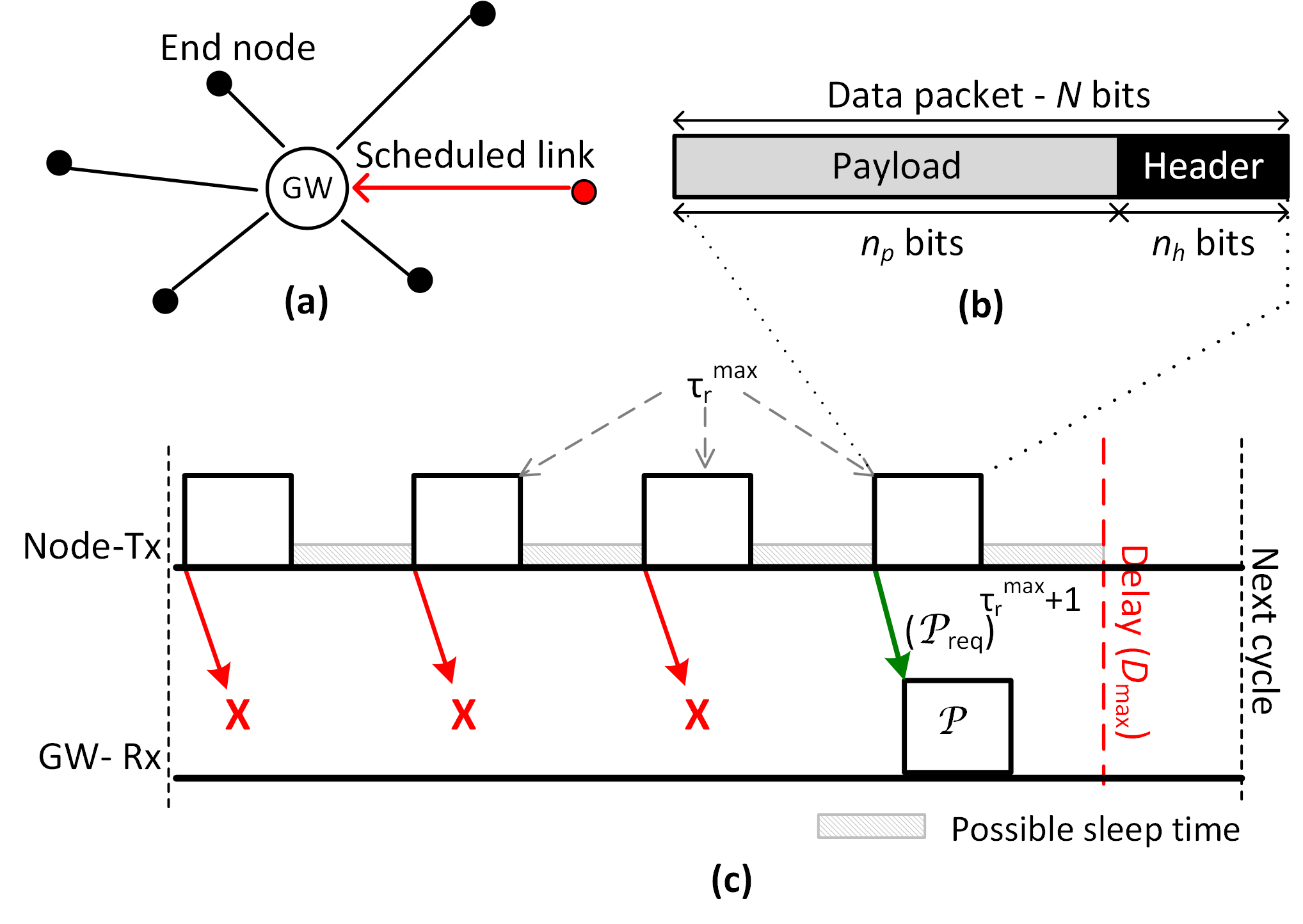
Figure 1: Network model: (a) network topology, (b) packet structure,(c) probabilistic service model: after $\tau_{r}^{\max}+1$ transmissions, a packet must be delivered within delivery deadline ($D_{\max}$) and reliability target ($\mathcal{P}$).

We consider a master-slave communication model, typical for industrial automation applications [21, 22]; a gateway (GW) acting as the master, and battery-operated wireless sensors as the slaves (see Fig. 1(a)). The sensors are placed at random locations within the communication range of the GW. The GW schedules a transmission by broadcasting a short control message, which indicates the sensor that shall transmit a packet exclusively in time and/or frequency resource. The control message also indicates the permissible maximum delay, $D_{\max}$, and the target packet error probability, $\mathcal{P}$, of the sanctioned transaction (see Fig. 1(c)). Note that the design of a scheduling policy that could satisfy the end-to-end latency including the delay in scheduling of a sensor is beyond the scope of this paper although one may refer to [4].

II-B Metrics, QoS Model and Objectives

In this work, we are interested in minimizing the energy consumption of the wireless sensor devices in transmitting the packet to the gateway. While optimizing the energy efficiency, we also want to ensure that the quality-of-service (QoS) requirements are fulfilled.

Energy efficiency metric. To capture the energy consumption and reliability trade-off, the cost-benefit of the link is expressed as the ratio of the energy consumption to the corresponding data reliably delivered as

$$E=\left(\frac{1}{1-p}\right)E_{0},$$ (1)

where the first term is the average number of transmissions, $\bar{\tau}$, over an i.i.d channel realizations between transmissions, which is the mean of a geometric random variable with parameter $p$–the packet error rate (PER). The term $E_{0}$, to be defined precisely in Sec. III, accounts for the energy consumed by the radio circuitry to operate the link. The measure unit of (1) is [$\mathrm{Joule}\text{/}\mathrm{bit}$] as it represents the amount of energy required to transmit a given amount of data or, as stated otherwise, the energy cost per reliably transmitted information bit.

The measure of energy consumption in (1), with its relation to PER, depends on the physical parameters as SNR or transmit power, modulation order and symbol rate, and MAC layer parameters including packet size—information and overhead bits (see Fig. 1(b))—and the number of retransmissions.

Energy efficiency metric with probabilistic QoS model. Since delay $D_{\max}$ is finite, the maximum number of retransmissions has to be bounded i.e., $\tau_{r}^{\max}=\left\lfloor{D_{\max}}/{t_{T}}\right\rfloor-1$ where $t_{T}$ is the transmission time of the packet. Moreover, due to finite retransmissions, an error-free delivery cannot be ensured. Since a packet loses its value after $D_{\max}$ in typical control applications, the packet is dropped after $\tau_{r}^{\max}$ retransmissions. Therefore, the condition: the probability of packet error after $\tau_{r}^{\max}$ retransmissions is not greater than $\mathcal{P}$, defines a probabilistic QoS model [23]

$$p^{\tau_{r}^{\max}+1}\leq\mathcal{P}.$$ (2)

Solving (2) for $p$ gives the reliability needed at the PHY layer under a limited number of retransmissions at the MAC layer

$$p\leq\mathcal{P}^{1/(\tau_{r}^{\max}+1)}:=\mathcal{P}_{\mathrm{req}}.$$ (3)

If (3) is satisfied for each transmission attempt at the physical layer, the application QoS requirement in (2) with maximum $\tau_{r}^{\max}$ retransmissions will be satisfied with the average number of transmissions per packet $\bar{\tau}_{\mathrm{trunc}}={1-p^{\tau_{r}^{\max}+1}}/{(1-p)}$. In this case, the energy consumption follows from (1) as

$$E_{\mathrm{trunc}}=\left(\frac{1-p^{\tau_{r}^{\max}+1}}{1-p}\right)E_{0}.$$ (4)

Objectives. From the above-defined probabilistic QoS model, our objective is to find the modulation scheme and its operational parameters: SNR at the PHY layer, and packet size at the MAC layer such that the required PER in (3) is satisfied by implementing $\tau_{r}^{\max}$ retransmissions at the MAC while energy efficiency in (4) for the sanctioned transaction is maximized.

III Elements of Energy Consumption Model

In this section, we define energy consumption model $E_{0}$, and derive it for various power amplifier models. Also, we find a PER expression that maintains an explicit connection with the modulation order and the associated parameters.

III-A Average Energy Per Information Bit

The energy consumption of the signal path between the transmitter and receiver is composed of baseband processing blocks and radio-frequency (RF) chain. The RF chain consists of a power amplifier (PA) and other electronic components such as analog-to-digital and digital-to-analog converters, low-noise amplifier, filters, mixers and frequency synthesizers. However, for an energy-constrained wireless system, the energy consumption of RF chain is the orders of magnitude higher than the consumption of baseband processing blocks. The power consumption of PA is considered to be proportional to the transmit power $P_{t}$ as $P_{\mathrm{PA}}=\xi P_{t}/\eta(P_{t})$, where $\xi$ is the modulation scheme dependent peak-to-average power ratio (PAPR) and $\eta(P_{t})$ is the $P_{t}$-dependent drain efficiency of the PA (see Sec. III-B). If baseband power consumption is neglected and the power consumption of all the other components in RF chain excluding PA is denoted as $P_{c}$, a simple power consumption model is $P_{\mathrm{on}}=\xi P_{t}/\eta(P_{t})+P_{c}$. From [11], it leads to total energy consumption to transmit and receive a symbol, $E_{\mathrm{sym}}$

$$E_{\mathrm{sym}}=\frac{\xi E_{t}}{\eta(P_{t})}+\frac{P_{c}}{R_{s}},$$ (5)

where $E_{t}$ is the average transmission energy of a symbol and $R_{s}$ is the symbol rate at PHY. For FSK, BPSK and QPSK modulations, PAPR $\xi=1$, for OQPSK $\xi=2.138$, and for a square MQAM modulations, it can be approximated as $\xi=3(\sqrt{M}-\frac{1}{\sqrt{M}}+1)$ [11].

Let $E_{b}={E_{r}}/{\log_{2}M}$ be the average received energy per uncoded bit, where $E_{r}$ is the average received energy per symbol and $M$ is the constellation size. Then, the average SNR ($\bar{\gamma}$) at the receiver is

$$\bar{\gamma}=\frac{E_{r}}{N_{0}\log_{2}M}.$$ (6)

Assuming a $\kappa$th-power path-loss model, the transmission energy at distance $d$ from (6) can be expressed as [11]

$$E_{t}\triangleq E_{r}G_{d}=\Big{(}\bar{\gamma}N_{0}\log_{2}M\Big{)}G_{d},$$ (7)

where $G_{d}\triangleq G_{1}d^{\kappa}M_{\ell}$ is the path-loss gain, where $G_{1}$ is the gain factor at unit distance, which depends on the transmit and receive antenna gains and carrier frequency, and $M_{l}$ is the link margin.

In a packet-based wireless system, the information bits are encapsulated into packets each carrying $n_{p}$ payload and $n_{h}$ overhead bits; thus the number of symbols in each packet are $n_{s}=(n_{h}+n_{p})/\log_{2}M$. Therefore, the average energy required to transmit and receive an information bit, from (5) and (7), is

$$E_{0}=\left(\frac{n_{p}+n_{h}}{n_{p}\log_{2}M}\right)E_{\mathrm{sym}}.$$ (8)

III-B $E_{0}$ for Different Power Amplifier Models

As PA is the most power consuming component of a wireless link, its real-life characteristics must be considered for energy efficient communication. The power consumption of PA is high mainly for its inefficiency in signal amplification, and non-linearity in signal amplification outside the limited dynamic range. As a result, if the PA input signal is higher than its linear region, the output signal is distorted; whereas, if PA input signal falls below from a saturation point—where the output power is maximum—the PA drain efficiency drops significantly. It is energy efficient to operate the PA at its saturation point [8], but because of the dynamic range of input signals (i.e., higher-order modulations with high PAPR), it cannot operate at the saturation point and the PA must back off at a certain output power.

In earlier studies, a PA model with constant drain efficiency is assumed (e.g., see [11, 16]), which is far from reality. To capture the trade-off in energy efficiency and reliability, the link dynamics under realistic PA models must be studied. In the following, we compare the constant PA (CPA) with two non-linear PA models: a) commonly used traditional PA (TPA) and, b) envelop tracking PA (ETPA) that uses a linear PA along with a supply modulation circuitry in which the supply voltage tracks the input signal envelope.

Constant PA. The drain efficiency $\eta$ of CPA is assumed to be constant irrespective of the output power $P_{t}$ i.e., $\eta(P_{t})=\eta_{0}$.

Traditional PA. Let $\eta(P_{t})$ be the drain or power efficiency of PA at the output power $P_{t}$, then it is given by [24]

$$\eta(P_{t})=\eta_{\max}\left(\frac{P_{t}}{P_{t,\max}}\right)^{\!\!1/2},$$ (9)

where $P_{t,\max}$ is the maximum designed output power and $\eta_{\max}$ is the maximum PA efficiency, which is achieved when $P_{t}=P_{t,\max}$.

At maximum output power e.g., $P_{t}=P_{0}$, a PA must be able to handle peak power, therefore $P_{0}\leq P_{t,\max}/\xi$. It means that, for instance, if PAPR of a modulation scheme is $8\text{\,}\mathrm{dB}\text{/}$ then $P_{0}$ must be $8\text{\,}\mathrm{dB}\text{/}$ less than $P_{t,\max}$.

Envelop tracking PA. For ET-PA, the power efficiency $\eta(P_{t})$ is modeled as [9]

$$\eta(P_{t})=\eta_{\max}\frac{P_{t}\left(1+c\right)}{P_{t}+cP_{t,\max}},$$ (10)

where $c=0.0082$ is a PA-dependent constant.

Fig. 2 depicts the efficiency response of these PA models. It can be clearly observed how unrealistic CPA model is from real-life PA models, while ETPA model is expected to improve energy efficiency in comparison with TPA.

Using these power efficiency relations, we derive energy consumption per information bit ($E_{0}$, (8)). Table I shows $E_{0}$ and its associated parameters for the consider PA models, where $R_{b}=W\log_{2}M$ is the PHY layer bit rate in bandwidth $W$.

TABLE I: Expressions For Energy Per Information Bit for Studied Power Amplifier Models

	CPA	TPA	ETPA
$E_{0}$	$\displaystyle\frac{n_{p}+n_{h}}{n_{p}}A\bar{\gamma}+B$	$\displaystyle\frac{n_{p}+n_{h}}{n_{p}}A\frac{\bar{\gamma}}{\sqrt{\bar{\gamma}}}+B$	Same as for CPA
$A$	$\displaystyle\frac{\xi N_{0}G_{d}}{\eta_{0}}$	$\displaystyle\frac{\xi N_{0}G_{d}\sqrt{P_{t,\max}}}{\eta_{\max}\sqrt{N_{0}G_{d}R_{b}}}$	$\displaystyle\frac{\xi N_{0}G_{d}}{\eta_{\max}\left(c+1\right)}$
$B$	$\displaystyle\frac{P_{c}}{R_{b}}$	$\displaystyle\frac{P_{c}}{R_{b}}$	$\displaystyle\frac{1}{R_{b}}\!\!\left(\!\frac{\xi cP_{t,\max}}{\eta_{\max}(c+1)}\!+\!P_{c}\!\!\right)$

Figure 2: Efficiency curves of different PA models, assuming $\eta_{\max}=$80\text{\,}\mathrm{\char 37\relax}\text{/}$$ and $P_{0}=$10\text{\,}\mathrm{dBm}\text{/}$$.

III-C Packet Error Rate

To minimize energy consumption per information bit $E$ in (1), we require a generic packet error rate (PER) approximation that is accurate and also maintains an explicit connection with the parameters defining the system performance. An accurate approximation for uncoded schemes is proposed in [25], which however cannot be utilized for optimizing the function $E$. Another, approximation is the upper bound on PER for (un)coded schemes in Rayleigh fading

$$\bar{P_{e}}\left(\bar{\gamma}\right)\leq 1-\mathrm{exp}\left(-\frac{\omega_{0}}{\bar{\gamma}}\right),$$ (11)

where $\bar{\gamma}$ is the SNR and $\omega_{0}$ is the waterfall threshold [26]. The threshold is defined as an integral of the PER function in the AWGN channel, $f\left(\gamma\right)$

$$\omega_{0}=\int_{0}^{\infty}{f\left(\gamma\right)d\gamma}.$$ (12)

For an $N$-bit uncoded packet with a bit error rate (BER) function $b_{e}\left(\gamma\right)$, $f\left(\gamma\right)$ is defined as

$$f(\gamma)=1-\Big{(}1-b_{e}\left(\gamma\right)\Big{)}^{N}.$$ (13)

A log-domain linear approximation of $\omega_{0}$ is proposed for uncoded schemes in [20], and for (un)coded schemes in [16]. However, the approximation in [20] is tight for large packets only while in [16] the approximation parameters for a given modulation scheme are calculated by simulations. On the other hand, the following new proposition shows that the waterfall threshold in (12) is tightly approximated by the expected value of an asymptotic distribution of $f(\gamma)$.

Proposition 1: For uncoded transmission of a packet with length $N$, with a BER function described by $c_{m}e^{-k_{m}\gamma}$ or $c_{m}Q(\sqrt{k_{m}\gamma})$ where $0<c_{m}\leq 1$ and $k_{m}>0$, the threshold, $\omega_{0}$, in Rayleigh fading channel is approximated by the expected value of the Gumbel distribution for sample maximum

$$\omega_{0}\approx{\mathbb{E}[\gamma]}\triangleq a_{N}+\gamma_{e}\,b_{N},$$ (14)

where $a_{N}$ and $b_{N}$ are the parameters of the Gumbel distribution, and $\gamma_{e}$ is the Euler constant.

Proof: See Appendix. $\blacksquare$

In [25], we have shown that the normalizing constants for BER functions of the form $c_{m}e^{-k_{m}\gamma}$ and $c_{m}Q(\sqrt{k_{m}\gamma})$ are

$$a_{N}=\frac{\log(Nc_{m})}{k_{m}},\,\,\,\,\,\,\,\,b_{N}=\frac{1}{k_{m}},$$ (15)

where the optimal parameters for the BER function $c_{m}Q(\sqrt{k_{m}\gamma})$ are $c_{m}\Rightarrow 0.2114c_{m}$ and $k_{m}\Rightarrow 0.5598k_{m}$ [1].

Inserting (14) and (15) in (11) leads to a simple PER approximation which maintains explicit connection with the modulation specific parameters ($c_{m}$, $k_{m}$), packet size ($N$) and SNR ($\bar{\gamma}$)

$$\bar{P}_{e}(\bar{\gamma})\approx 1-\big{(}N\big{)}^{-\frac{1}{k_{m}\bar{\gamma}}}\mathrm{exp}\left(-\frac{\log c_{m}+\gamma_{e}}{k_{m}\bar{\gamma}}\right).$$ (16)

The PER approximation in (16) tightly matches to the upper bound, as compared to existing solutions for any modulation scheme with the BER function in the form of exponential and the Gaussian-$Q$ function. In order to show the accuracy of proposed approximation, using as an example of uncoded 16 QAM, Fig. 3 compares it with the numerical evaluation of (11), and also with the prior approximations in terms of relative error (RE) with respect to real PER. The real PER is found by the numerical integration of (13) over Rayleigh fading distribution. It can be observed that the RE of the proposed approximation is close to the upper bound (11) for small to large packet lengths. In comparison, the RE of approximations in [16][20] is small at low SNR, however it increases rapidly especially for small packet lengths.

Figure 3: Relative error (RE) in average PER for 16 QAM modulation in Rayleigh fading.

PER for Coded Schemes. We can easily use the approximation (16) for PER evaluation of coded schemes by equating $k_{M}=1/k_{m}$, and $b_{M}=\left(\log c_{m}+\gamma_{e}\right)/k_{m}$, where $k_{M}$ and $b_{M}$ are calculated by simulations for various coded schemes in [16, Table I]. Therefore, one can perform the energy-reliability analysis presented in this paper for coded schemes as well. However, as the low-cost and low-power IoT devices rely on retransmissions instead of error-correction to reduce the system complexity [7], we adhere to uncoded schemes to be compatible with low-cost IoT devices.

IV Link Optimization with Minimum Energy Consumption

With two main components of our objective function $E$ in place, now we find energy optimal yet QoS-aware (i.e., maintaining the PER constraint in (3)) PHY and MAC parameters.

IV-A Optimal Average SNR / Transmit Power

To find an energy-optimal SNR, we fix the packet payload $n_{p}$. It also represents a case where the sensors have to send fixed-size reports. Moreover, the optimal SNR must satisfy the reliability constraints set via PER and the constraints on the maximum transmit power, which could be either due to hardware limitations or frequency band regulations. Therefore, the optimization of objective function (1) with respect to SNR $\bar{\gamma}$ can be written as

$$\underset{\bar{\gamma}}{\text{minimize}} E(\bar{\gamma})$$ (17)

subject to $$\bar{\gamma}_{\min}\leq\bar{\gamma}\leq\bar{\gamma}_{\max},$$

where $\bar{\gamma}_{\min}$ is the minimum average SNR requirement under PER bound in (3). From (16), $\bar{\gamma}_{\min}$ is

$$\bar{\gamma}_{\min}=-\frac{\gamma_{e}+\log\Big{(}c_{m}\left(n_{h}+n_{p}\right)\Big{)}}{k_{m}\log\left(1-\mathcal{P}_{\mathrm{req}}\right)}.$$ (18)

While $\bar{\gamma}_{\max}$ is the maximum achievable SNR at transmit power limit $P_{0}$. Since the transmit power $P_{t}$ cannot exceed $P_{0}$, i.e., $P_{\mathrm{t}}\leq P_{0}$, it translates to $\bar{\gamma}\leq\bar{\gamma}_{\max}$ with $\bar{\gamma}_{\max}$ from (7) as

$$\bar{\gamma}_{\max}=\frac{P_{0}}{WN_{0}G_{d}}.$$ (19)

From (18) and (19), the required SNR, denoted as $\bar{\gamma}^{*}_{\mathrm{req}}$, relates to an unconstrained optimal SNR $\bar{\gamma}^{*}$ as

$$\bar{\gamma}^{*}_{\mathrm{req}}=\begin{dcases}\bar{\gamma}_{\min},&\bar{\gamma}^{*}<\bar{\gamma}_{\min}\\ \bar{\gamma}_{\max},&\bar{\gamma}^{*}>\bar{\gamma}_{\max}\\ \,\,\bar{\gamma}^{*},&\mathrm{otherwise}\\ \end{dcases}$$ (20)

which holds only if the condition $\bar{\gamma}_{\min}<\bar{\gamma}_{\max}$ is satisfied. Otherwise, the reliability target cannot be satisfied for a given modulation scheme because of transmit power constraint.

The conditions in (20) can be visualized with Fig. 4, which is obtained using the parameters in Sec. V Table. II under constant PA. Fig. 4 shows an example case of minimum required SNR $\bar{\gamma}_{\min}$ to satisfy certain QoS at various distances. It also depicts the unconstrained optimal SNR $\bar{\gamma}^{*}$ and maximum achievable SNR $\bar{\gamma}_{\max}$. At $d=$10\text{\,}\mathrm{m}\text{/}$$, $\bar{\gamma}_{\min}$ is less than $\bar{\gamma}^{*}$, therefore $\bar{\gamma}^{*}$ is energy optimal and is preferred over $\bar{\gamma}_{\min}$. While at $d=$30\text{\,}\mathrm{m}\text{/}$$, $\bar{\gamma}^{*}$ cannot satisfy the target and $\bar{\gamma}_{\min}$, though not energy optimal, is selected. At $d=$70\text{\,}\mathrm{m}\text{/}$$, the reliability target is not satisfied as $\bar{\gamma}_{\min}>\bar{\gamma}_{\max}$.

Figure 4: Comparison of optimal, required and maximum achievable SNRs at different distances ($d$) for 4-QAM under reliability constraints of $\mathcal{P}=$0.001$$, $\tau_{r}^{\max}=$3$$, $n_{p}=$976\text{\,}\mathrm{bit}\text{/}$$ and maximum transmit power $P_{0}=$10\text{\,}\mathrm{mW}\text{/}$$.

We can find $\bar{\gamma}^{*}$, which is finally conditioned by (20), based on the following unconstrained optimization problem

$$\underset{\bar{\gamma}}{\text{minimize}} E(\bar{\gamma})$$ (21)

subject to $$\bar{\gamma}\in\left[0,\infty\right].$$

Note that $E(\bar{\gamma})$ is a product of two functions: the number of retransmissions $\bar{\tau}(\gamma)$ with $\bar{\tau}^{{}^{\prime}}(\gamma)\leq 0$, and the average energy per transmission attempt $E_{0}(\gamma)$ such that $E_{0}^{{}^{\prime}}(\gamma)\geq 0$ where $\acute{x}$ denotes the first derivative. Given that both $\bar{\tau}(\gamma)$ and $E_{0}(\gamma)$ are convex, the function $E(\bar{\gamma})$ is also convex [16, Lemma 1].

CPA/ETPA model. For CPA/ETPA model with $E_{0}$ in Table I, $\bar{\gamma}^{*}$ can be obtained by solving $\frac{\partial E}{\partial\bar{\gamma}}=0$ in (21), which yields a quadratic equation with a positive root as

$$\bar{\gamma}^{*}=\frac{\omega_{0}}{2}+\sqrt{\omega_{0}\left(\frac{\omega_{0}}{4}+\frac{B}{A}\frac{n_{p}}{n_{h}+n_{p}}\right)}.$$ (22)

TPA model. For $E_{0}$ with TPA model in Table I, although $E$ is convex, the optimal $\bar{\gamma}^{*}$ is not found explicitly. However, it can be determined numerically from the following non-quadratic equation

$$Ak_{m}\left(\bar{\gamma}\right)^{3/2}-2A\omega_{0}(\bar{\gamma})^{1/2}-{2\omega_{0}B}\left(\frac{n_{p}}{{n_{p}+n_{h}}}\right)=0,$$ (23)

which has a real positive root if the condition $\!27B^{2}k_{m}\left({n_{p}}/{(n_{p}\!+\!n_{h})}\right)^{2}>8A^{2}\omega_{0}$ is satisfied

$$\bar{\gamma}^{*}=\frac{1}{3}\left(\frac{4\omega_{0}}{k_{m}}\,\,+\,\,\frac{4\omega_{0}^{2}}{\mathcal{A}^{\frac{1}{3}}}\,\,+\,\,\frac{\mathcal{A}^{\frac{1}{3}}}{k_{m}^{2}}\right),$$ (24)

where

$$\mathcal{A}= \frac{1}{A^{2}}\bigg{[}54B^{2}k_{m}^{4}\omega_{0}^{2}\Big{(}\frac{n_{p}}{n_{p}\!+\!n_{h}}\Big{)}^{\!\!2}-8A^{2}k_{m}^{3}\omega_{0}^{3}+6\sqrt{3}\,\,\times$$

$$\!\!\!\left(\!B^{2}k_{m}^{7}\omega_{0}^{4}\Big{(}\frac{n_{p}}{n_{p}\!+\!n_{h}}\Big{)}^{\!\!2}\Big{(}\!27B^{2}k_{m}\Big{(}\frac{n_{p}}{n_{p}\!+\!n_{h}}\Big{)}^{\!\!2}\!-\!8A^{2}\omega_{0}\!\Big{)}\!\right)^{\!\frac{1}{2}}\!\bigg{]}.$$

IV-B Optimal Packet Payload

Now we find the optimal $n_{p}$—the payload that minimizes the objective function (1)—by keeping SNR constant. The upper limit on the maximum payload size ${n_{p,\max}}$ is determined by required $\bar{\gamma}_{\min}$ to satisfy a PER target. Therefore, our objective function is

$$\underset{\bar{\gamma}}{\text{minimize}} E(n_{p})$$ (25)

subject to $$0\leq n_{p}\leq n_{p,{\max}},$$

where $n_{p,{\max}}$, from (3), is

$${n_{p,\max}}=-n_{h}+\frac{1}{c_{m}}10^{\displaystyle{-\big{(}\gamma_{e}+\bar{\gamma}_{\min}k_{m}\log\left(1-\mathcal{P}_{\textrm{req}}\right)\big{)}}},$$ (26)

with $\bar{\gamma}_{\min}$ defined in (18). After reliability condition known with respect to maximum payload size, $n_{p}^{*}$ obtained via unconstrained optimization of $E(n_{p})$ can easily be conditioned i.e., if $n_{p}^{*}>n_{p,{\max}}$ then $n_{p}=n_{p,{\max}}$ and otherwise $n_{p}=n_{p}^{*}$.

The function $E(n_{p})$ is convex in $n_{p}$ and the unconstrained optimal $n_{p}^{*}$ for the considered PA models is given below.

CPA/ETPA model. In case of ETPA, the optimal $n_{p}^{*}$ is determined as

$$n_{p}^{*}=\!\!\frac{n_{h}\bar{\gamma}\left(\left(k_{m}\!-1\right)\bar{\gamma}\!+\!\sqrt{k_{m}^{2}\bar{\gamma}^{2}\!+\!2k_{m}\bar{\gamma}\!+\!\frac{4Bk_{m}}{A}\!+\!1}\right)}{2\Big{(}\bar{\gamma}+\frac{B}{A}\Big{)}}.$$ (27)

TPA model. For TPA, $n_{p}^{*}$ is

$$n_{p}^{*}=\frac{n_{h}\mathcal{K}+\sqrt{4Ak_{m}n_{h}^{2}\bar{\gamma}\left(A\bar{\gamma}-B\sqrt{\bar{\gamma}}\right)\left(\bar{\gamma}-\frac{B^{2}}{A^{2}}\right)-n_{p}^{2}\mathcal{K}^{2}}}{2A\left(\bar{\gamma}-\frac{B^{2}}{A^{2}}\right)},$$ (28)

where $\mathcal{K}=Ak_{m}\bar{\gamma}^{2}-Bk_{m}\bar{\gamma}^{3/2}-A\bar{\gamma}+B\sqrt{\bar{\gamma}}$.

IV-C Joint Energy Optimal Parameters—$\bar{\gamma},n_{p},M,\tau_{r}^{\max}$

As the IoT devices will be used in diverse monitoring and control applications, it might be important in many to find the optimal SNR, payload size, modulation order and the number of retransmissions for energy efficient communication. For example, after deployment in harsh and inaccessible areas, the devices can optimize these parameters at the start of their operation and then continue with the optimal link setting. The problem to jointly optimization these parameters can be formulated as

$$\underset{\bar{\gamma},n_{p},M,\tau_{r}^{\max}}{\text{minimize}} E\Big{(}\bar{\gamma},n_{p},M,\tau_{r}^{\max}\Big{)},$$ (29)

where $M\in\{\mathrm{FSK,MPSK,MQAM}\}$ and $\tau_{r}^{\max}=i,\;i\geq 1$. Note that the IoT devices will support only a few modulation schemes $M$. In addition, a small value of maximum retransmissions $\tau_{r}^{\max}$ is feasible for operation with minimum energy consumption [16]. As a result, an exhaustive search over the combination of $M$ and $\tau_{r}^{\max}$ will not be computationally demanding.

On the other hand, for each combination of $M$ and $\tau_{r}^{\max}$, the joint optimum of $\bar{\gamma}$ and $n_{p}$ can be found from (22) and (27) either by solving a system of two non-linear equations or by iteratively invoking these equations. In either case, we must ensure that the reliability conditions in (20) and (26) are satisfied. However, the former approach requires numerical evaluation that might not be computationally feasible for hardware-constrained IoT devices. Whereas, by iteratively invoking (22) and (27), $\bar{\gamma}$ and $n_{p}$ can efficiently converge to joint energy optimum values while satisfying the reliability conditions. It is straightforward to develop the proof of convergence of the iterative approach [16, Corollary 3] under the probabilistic QoS model. We observed that by initializing $n_{p}$ and $\bar{\gamma}$ to any random values, this approach converges to their optimum values within a few iterations.

A pseudocode of the proposed joint optimization of (29) is given in Algorithm 1. At a given distance, the algorithm iterates over all combinations of $M$ and $\tau_{r}^{\max}$ while for each combination, $\bar{\gamma}$ and $n_{p}$ are evaluated iteratively. The convergence of $\bar{\gamma}$ and $n_{p}$ is monitored with the residual SNR $\Delta>\delta$, where $\delta$ is the precision tolerance.

Algorithm 1 Joint Energy-Reliability Aware Optimization of a Link’s Parameters

0:  $\mathcal{P}_{\mathrm{req}},\tau_{r}^{\max},\delta$

0:  $\bar{\gamma}^{*},n_{p}^{*},\tau_{r}^{*},M^{*}$

1:  for $M\in\left[\mathrm{FSK,MPSK,MQAM}\right]$ do

2:     for $i=1$ to $\tau_{r}^{\max}$ do

3:        $n_{p}\leftarrow 0$

4:        while $\Delta>\delta$ do

5:           $\bar{\gamma}\leftarrow$ Evaluate (22) or (23), $\bar{\gamma}_{\min}\leftarrow$ Evaluate (18), $\bar{\gamma}_{\max}\leftarrow$ Evaluate (19), $n_{p,{\max}}\leftarrow$ Evaluate (26)

6:           if ($\bar{\gamma}_{\min}>\bar{\gamma}_{\max}$) then

7:              $\mathrm{break}$;

8:           else

9:              $\bar{\gamma}_{\mathrm{req}}\leftarrow$ Evaluate (20)

10:           end if

11:           $n_{p}\leftarrow$ Evaluate (27) or (28) with $\bar{\gamma}$ = $\bar{\gamma}_{\mathrm{req}}$

12:           if $(n_{p}>n_{p,{\max}})$ then

13:              $n_{p}\leftarrow n_{p,{\max}}$

14:           end if

15:           $E\leftarrow$ Evaluate (4), Print $E,{\gamma},n_{p},\tau_{r},M$ $\Delta\leftarrow|\bar{\gamma}_{\mathrm{req}}-\bar{\gamma}^{{}^{\prime}}|,\,\,\bar{\gamma}^{{}^{\prime}}=\bar{\gamma}_{\mathrm{req}}$

16:        end while

17:     end for

18:  end for

19:  return  $\bar{\gamma},n_{p},\tau_{r},M$ giving minimum $E$

V Numerical Results

In this section, we present the numerical results of the proposed link optimization approach. The parameters used for the numerical analysis are given in Table II, where the PER target of $\mathcal{P}=$0.001$$ translates to $99.9\text{\,}\mathrm{\char 37\relax}\text{/}$ reliability.

TABLE II: Parameters for Numerical Analysis

Parameter	Symbol	Value
Max. transmit power	$P_{0}$	$10\text{\,}\mathrm{mW}\text{/}$
Noise power density	$N_{0}/2$	$-174\text{\,}\mathrm{dBm}\text{/}\mathrm{Hz}$
Path loss exponent	$\kappa$	$3.5$
Path gain at unit distance	$G_{1}$	$30\text{\,}\mathrm{dB}\text{/}$
Link margin	$M_{\ell}$	$40\text{\,}\mathrm{dB}\text{/}$
Bandwidth	$W$	$10\text{\,}\mathrm{kHz}\text{/}$
Circuit power - MQAM, MFSK	$P_{c}$	$310\text{\,}\mathrm{mW}\text{/}$, $265\text{\,}\mathrm{mW}\text{/}$
Max. PA efficiency	$\eta_{0},{\eta_{\max}}$	$80\text{\,}\mathrm{\char 37\relax}\text{/}$
Packet overhead	$n_{h}$	$48\text{\,}\mathrm{bit}\text{/}$
Target PER	$\mathcal{P}$	$0.001$
Max. retransmission	$\tau_{r}^{\max}$	$3$
Precision tolerance	$\delta$	$10^{-6}$

When operated at the optimal SNR and payload size, the energy consumption (EC) of the selected modulation schemes with respect to distance with (solid lines) and without (dotted-marker lines) reliability constraints is shown in Fig. 5. These results are obtained based on constant PA. It is observed that there is an energy-optimal modulation scheme at each distance that also satisfies the reliability target: higher-order modulations at lower distance and lower-order at higher distance. However, for a given transmit power limit, the distance until which the reliability target is satisfied decreases as the reliability requirements get tight. Also, how energy efficiency takes a toll under reliability constraints, compared to a link with unlimited allowed transmissions, can also be noticed especially for higher-order modulations. Note that the EC gap increases with reliability constraints becoming stringent. This is because, to meet the reliability target, the parameters other than the energy-optimal ones are selected. We observed the similar EC trend for other PA models however with exceptions that need in-depth analysis.

Figure 5: Energy consumption of various modulation schemes under CPA model with optimal SNR ($\bar{\gamma}^{*}$) and payload ($n_{p}^{*}$) at each distance. Reliability parameters: $\mathcal{P}=$0.001$$, $\tau_{r}^{\max}=$3$$. The dotted-marker curves ($\cdot\cdot$+$\cdot\cdot$) show the energy consumption without any reliability constraints.

Using Algorithm 1, Fig. 6 gives a holistic view of how energy-optimal parameters—modulation size ($M$), SNR ($\bar{\gamma}$) or transmit power ($P_{t}$), payload ($n_{p}$) and the number of retransmissions ($\tau_{r}$)—vary with the link distance. Mainly, it compares the impact of PA models on the EC while closely looking at the optimal system parameters. Fig. 6LABEL:sub@fig:1a shows that the EC under constant PA (CPA)-model is considerably optimistic compared to realistic PA models. Although the EC for envelope-tracking PA (ETPA) is higher and closely follows the EC for CPA, it is considerably higher for traditional PA (TPA). As a result, TPA model sees a link switching to a low-order modulation at shorter distances. Thus, TPA reduces the gain in using high-order modulation for a device using only OQPSK modulation.

(a) Energy consumption ($E$)

(b) Optimal transmit power ($P_{t}$) and PA power consumption ($P_{\textrm{pa}}$)

(c) Optimal SNR ($\bar{\gamma}$)

(d) Optimal payload ($n_{p}$)

(e) Optimal no. of retransmissions ($\tau_{r}$)

Figure 6: Impact of PA models on energy consumption and optimal PHY/MAC parameters. Figures (a) and (b) are essentially reciprocal results for $\bar{\gamma}$ and $P_{t}$, respectively, while (b) shows additional information on PA power consumption ($P_{\textrm{pa}}$).

In Fig. 6LABEL:sub@fig:1b–Fig. 6LABEL:sub@fig:1d, we can observe the trade-off or inter-play among the link parameters in minimizing EC under ETPA and TPA, where the parameters under CPA are omitted for the clarity of figures. Nevertheless, their trend is similar to the link parameters for ETPA. In general, the behavior of these parameters must be interpreted together with the PA-efficiency curves in Fig. 2. It can be noticed that, for a device at short distances, higher-order modulation and high-power transmissions are energy efficient under ETPA. Although ETPA has a higher power consumption ($P_{pa}=\xi P_{t}/\eta(P_{t})$) than TPA at the same distances (see Fig. 6LABEL:sub@fig:1b-(top) for distance between $1\text{\,}\mathrm{m}\text{/}11\text{\,}\mathrm{m}\text{/}$), thanks to better linearity of ETPA, high-power transmissions are capitalized by the device to successfully transfer (small-sized) information bits with a low number of retransmissions. Whereas, the power consumption of TPA is smaller but, with the increase in distance, it causes the increase in EC at a higher rate than the ETPA. As a result, TPA leads to almost third modulation degradation (i.e., to OQPSK) while 64 QAM is still energy optimal under ETPA. The reason behind low energy efficiency of TPA can be explained from its inefficiency at low output powers. To compensate for the limited gain in transmitting at high-power at short distances, the device opt for small transmit power but with a higher payload size and a higher number of retransmissions.

In general, the order of optimal modulation reduces as the distance increases. However with ETPA, at distances around $11\text{\,}\mathrm{m}\text{/}24\text{\,}\mathrm{m}\text{/}$, 16 QAM achieves better energy efficiency than TPA owing to its better trade-off in efficiency and the other link parameters (as discussed earlier). An interesting observation in this range is the rapid increase in payload size with the distance, which starts at around $17\text{\,}\mathrm{m}\text{/}$. However, note that, the corresponding SNR (in Fig. 6LABEL:sub@fig:1c) remains constant in this distance range. That is because increasing the transmit power with increasing packet size is optimal until next smaller modulation becomes energy optimal. If observed carefully, a small jump in payload size before the ETPA link downgrades its modulation from 64 QAM to 16 QAM can also be noticed.

When comparing the results where the same modulation scheme is employed under both the ETPA and TPA (i.e., at distances $\geq$$24\text{\,}\mathrm{m}\text{/}$), it can be observed that both transmit power and power consumption for TPA jumps higher than ETPA for the first time and their corresponding EC become almost identical. This is because the TPA efficiency increase exponentially in this range of output power, and also the small PAPR of OQPSK modulation reduces the amount of back off from the saturation region. As a consequence, this has an effect on the link parameters under TPA where the payload starts reducing with the distance and the number of retransmissions also reduce at some distances. However, as soon as the link operates at its maximum allowed transmit power, the link parameters under two PAs, including the modulation scheme (i.e., BPSK), become identical.

V-A Lifetime Analysis of IoT Links/Devices

The optimal link parameters, as discussed earlier, allow analyzing the lifetime of IoT devices while considering their non-ideal hardware characteristics. For the analysis, we assume that each device is battery-powered, and it reserves a charge capacity of $2\text{\,}\mathrm{A}\text{/}$$\text{\,}\mathrm{h}$ only for data communication. Also, each device, located at a certain distance from the gateway, is assumed to be transmitting $5\text{\,}\mathrm{kbit}\text{/}$ of sensory data on the average within a period of $5\text{\,}\mathrm{min}\text{/}$.

Fig. 7 shows the lifetime of a device with respect to link distance for the studied PA models, when operated with the optimized link parameters. It also depicts the lifetime of a device using only OQPSK modulation while the selection of other link parameters at any distance is energy-reliability optimal. We observe that spectral efficient modulations can significantly prolong the lifetime of the devices located at short-range distances, i.e., within $1\text{\,}\mathrm{m}\text{/}24\text{\,}\mathrm{m}\text{/}$ under CPA and ETPA. The expected lifetime increases as the distance decreases, and compared to a commonly used low-order modulation (i.e., OQPSK) in IoT devices, the lifetime can be extended up to $180\text{\,}\mathrm{\char 37\relax}\text{/}$ in case of an ideal PA and $125\text{\,}\mathrm{\char 37\relax}\text{/}$ for ETPA. On the other hand, traditional PA (TPA) not only halves the range in which a high-order modulation can help in extending the device/link life, it also brings down the gain in using higher-order modulations significantly.

VI Conclusions

We studied cross-layer optimization of battery-operated wireless links with energy consumption (EC) minimization objective while considering: (a) reliability requirements of IoT applications, and (b) operational constraints and non-ideal characteristics of the IoT devices’ hardware. To this end, we derived EC models while capturing energy cost of ideal and realistic power amplifiers (PAs), and packet error statistics in particular. For packet error statistics, we developed an accurate PER approximation in Rayleigh block-fading, which is simple to exploit for cross-layer link design and optimization. Using the EC models, we derived energy-optimal, reliability-aware, and hardware-compliant conditions for SNR and payload size, which we exploited for developing a holistic algorithm to optimize the link parameters jointly. The algorithm can be utilized by resource-constrained devices for link adaptation based on the optimal selection of parameters.

Our path to link optimization allowed to make useful observations, especially when the target is to simultaneously minimize energy consumption and ensure certain reliability. We found that at each distance there is an optimal SNR and payload size, which leads to an energy optimal modulation scheme where the modulation order increases for short-range links. However a reliability-aware link compared to a delay tolerant system reduces this distance, and increases the energy consumption. Also, when non-realistic power amplifier (PA) characteristics are considered, we found that the traditional PA significantly diminishes the gain in the usage of higher-order modulations (causing both the higher energy consumption for higher-order modulations, and switching to smaller modulations at shorter distances). While an envelop-tracking PA behaves closely to an ideal PA. Since the higher-order modulations offer packing more information bits, they are energy-optimal at short distances, because circuit power exceeds PA power consumption. However, PA’s non-linearity makes these powers comparable and leads to a higher energy consumption compared to an ideal PA.

Our lifetime analysis found that under ideal PA the lifetime can be extended up to $180\text{\,}\mathrm{\char 37\relax}\text{/}$ by selecting higher-order modulations in short-range networks compared to OQPSK. However, this gain reduces significantly under traditional PA, and the distance up to which a higher-order modulation can provide any gain reduces to half. Whereas, the envelop-tracking PA can still provide the lifetime extension of up to $125\text{\,}\mathrm{\char 37\relax}\text{/}$. These results highlight the need to investigate efficient PAs for short-range IoT networks in order to gain from spectral efficient modulations.

As a future work, the presented link optimization under non-linear PAs can be refined for relay selection and transmission duty-cycle optimization in an IoT system, as in [27].

Figure 7: Lifetime analysis of a device transmitting on average $5\text{\,}\mathrm{kbit}\text{/}$ of sensor data every $5\text{\,}\mathrm{min}\text{/}$. Reliability parameters: $\mathcal{P}=$0.001$$, $\tau_{r}^{\max}=$3$$, Other parameters: $P_{0}=$10\text{\,}\mathrm{mW}\text{/}$$, $n_{h}=$48\text{\,}\mathrm{bit}\text{/}$$, $\eta_{\max}=$80\text{\,}\mathrm{\char 37\relax}\text{/}$$.

[Proof of Proposition 1] For an $N$-bit packet, the PER function in (13) for BER functions described by $c_{m}e^{-k_{m}\gamma}$ and $c_{m}Q(\sqrt{k_{m}\gamma})$ is asymptotically approximated by the Gumbel distribution function for the sample minimum [25]

$$f(\gamma)\simeq 1-\mathrm{exp}\left(-\mathrm{exp}\left(-\frac{\gamma-a_{N}}{b_{N}}\right)\right),$$ (30)

where $a_{N}$ and $b_{N}>0$ are the normalizing constants.

Let $G\left(\gamma\right)=\mathrm{exp}(-\mathrm{exp}(-\frac{\gamma-a_{N}}{b_{N}}))$ be the cumulative distribution function (CDF) of the Gumbel distribution for the sample maximum, then from (30) and (12) we have

$$\omega_{0}\approx\int_{0}^{\infty}{\left(1-G\left(\gamma\right)\right)d\gamma},$$ (31)

which is the expected value of a continuous and non-negative random variable $\gamma$.

References

- [1] A. Mahmood, M. M. A. Hossain, and M. Gidlund, “Cross-layer optimization of wireless links under reliability and energy constraints,” in IEEE WCNC, Apr 2018, pp. 1–6.
- [2] H. Shariatmadari, R. Ratasuk, S. Iraji, A. Laya, T. Taleb, R. Jäntti, and A. Ghosh, “Machine-type communications: current status and future perspectives toward 5G systems,” IEEE Commun.Mag., vol. 53, no. 9, pp. 10–17, Sep 2015.
- [3] G. Durisi, T. Koch, and P. Popovski, “Toward massive, ultrareliable, and low-latency wireless communication with short packets,” Proc. of IEEE, vol. 104, no. 9, pp. 1711–1726, Sep 2016.
- [4] Y. Chen, H. Zhang, N. Fisher, L. Y. Wang, and G. Yin, “Probabilistic per-packet real-time guarantees for wireless networked sensing and control,” IEEE Trans. Ind. Informat., vol. 14, no. 5, pp. 2133–2145, May 2018.
- [5] B. Martinez, M. Montón, I. Vilajosana, and J. D. Prades, “The power of models: Modeling power consumption for IoT devices,” IEEE Sensors J., vol. 15, no. 10, pp. 5777–5789, Oct 2015.
- [6] X. Chen, Y. Xu, and A. Liu, “Cross layer design for optimizing transmission reliability, energy efficiency, and lifetime in body sensor networks,” Sensors, vol. 17, no. 4, 2017.
- [7] T. Shafique, A. M. Abdelhady, O. Amin, and M. Alouini, “Energy efficiency, spectral efficiency and delay analysis for selective ARQ multichannel systems,” IEEE Trans. Green Commun. Netw., vol. 2, no. 3, pp. 612–622, Sep 2018.
- [8] J. Joung, C. K. Ho, K. Adachi, and S. Sun, “A survey on power-amplifier-centric techniques for spectrum- and energy-efficient wireless communications,” IEEE Commun. Surveys Tuts., vol. 17, no. 1, pp. 315–333, Firstquarter 2015.
- [9] M. A. Hossain and R. Jäntti, “Impact of efficient power amplifiers in wireless access,” in IEEE Online Conf. on Green Communications, 2011, pp. 36–40.
- [10] Q. Cui, Y. Zhang, W. Ni, M. Valkama, and R. Jäntti, “Energy efficiency maximization of full-duplex two-way relay with non-ideal power amplifiers and non-negligible circuit power,” IEEE Trans. W. Commun., vol. 16, no. 9, pp. 6264–6278, Sep 2017.
- [11] S. Cui, A. J. Goldsmith, and A. Bahai, “Energy-constrained modulation optimization,” IEEE Trans. W. Commun., vol. 4, no. 5, pp. 2349–2360, 2005.
- [12] T. Wang, W. Heinzelman, and A. Seyedi, “Minimization of transceiver energy consumption in wireless sensor networks with AWGN channels,” in 46th Conf. on Commun., Control, and Computing, 2008, pp. 62–66.
- [13] Y. Hou, M. Hamamura, and S. Zhang, “Performance tradeoff with adaptive frame length and modulation in wireless network,” in 5th Intl. Conf. on Computer and Inf. Tech., 2005, pp. 490–494.
- [14] F. Rosas and C. Oberli, “Modulation and SNR optimization for achieving energy-efficient communications over short-range fading channels,” IEEE Trans. W. Commun., vol. 11, no. 12, pp. 4286–4295, 2012.
- [15] R. S. Prabhu and B. Daneshrad, “Energy minimization of a QAM system with fading,” IEEE Trans. W. Commun., vol. 7, no. 12, pp. 4837–4842, Dec 2008.
- [16] J. Wu, G. Wang, and Y. R. Zheng, “Energy efficiency and spectral efficiency tradeoff in type-I ARQ systems,” IEEE J. Sel. A. in Commun., vol. 32, no. 2, pp. 356–366, 2014.
- [17] M. Holland, T. Wang, B. Tavli, A. Seyedi, and W. Heinzelman, “Optimizing physical-layer parameters for wireless sensor networks,” ACM Trans. Sen. Netw., vol. 7, no. 4, pp. 28:1–28:20, Feb. 2011.
- [18] E. Sisinni, A. Saifullah, S. Han, U. Jennehag, and M. Gidlund, “Industrial internet of things: Challenges, opportunities, and directions,” IEEE Trans. Indus. Informat., vol. 14, no. 11, pp. 4724–4734, Nov 2018.
- [19] A. Zappone, L. Sanguinetti, and M. Debbah, “Energy-delay efficient power control in wireless networks,” IEEE Trans. Commun., vol. 66, no. 1, pp. 418–431, Jan 2018.
- [20] S. Liu, X. Wu, Y. Xi, and J. Wei, “On the throughput and optimal packet length of an uncoded ARQ system over slow Rayleigh fading channels,” IEEE Commun. Lett., vol. 16, no. 8, pp. 1173–1175, 2012.
- [21] S. Vitturi, L. Seno, F. Tramarin, and M. Bertocco, “On the rate adaptation techniques of IEEE 802.11 networks for industrial applications,” IEEE Trans. Indus. Informat., vol. 9, no. 1, pp. 198–208, Feb 2013.
- [22] Q. Wang and J. Jiang, “Comparative examination on architecture and protocol of industrial wireless sensor network standards,” IEEE Commun. Surveys Tuts., vol. 18, no. 3, pp. 2197–2219, thirdquarter 2016.
- [23] Q. Liu, S. Zhou, and G. B. Giannakis, “Cross-layer combining of adaptive modulation and coding with truncated ARQ over wireless links,” IEEE Trans. W. Commun., vol. 3, no. 5, pp. 1746–1755, 2004.
- [24] K. Han, Y. Choi, S. Choi, and Y. Kwon, “Power amplifier characteristic-aware energy-efficient transmission strategy,” Lecture Notes in Computer Science, vol. 4479, p. 37, 2007.
- [25] A. Mahmood and R. Jäntti, “Packet error rate analysis of uncoded schemes in block-fading channels using extreme value theory,” IEEE Commun. Lett., vol. 21, no. 1, pp. 208–211, Jan 2017.
- [26] Y. Xi, A. Burr, J. Wei, and D. Grace, “A general upper bound to evaluate packet error rate over quasi-static fading channels,” IEEE Trans. W. Commun., vol. 10, no. 5, pp. 1373–1377, 2011.
- [27] J. Tan, A. Liu, M. Zhao, H. Shen, and M. Ma, “Cross-layer design for reducing delay and maximizing lifetime in industrial wireless sensor networks,” EURASIP J. Wirel. Commun. Netw., vol. 2018, no. 1, p. 50, 2018.