A mesoscopic model for the effective electrical conductivity of composite polymeric electrolytes

Abstract

The effective quasistatic conductivity of composite polymeric electrolytes is studied in terms of a hard-core–penetrable-layer model. Used to incorporate the interface phenomena (such as amorphization of the polymer matrix around filler particles, stiffening effect by those on the amorphous phase, irregularities of the filler grains’ surfaces, etc.), the layers are assumed to be electrically inhomogeneous, consisting of a finite or infinite number of concentric uniform shells. The rules of dominance, imposed on the overlapping regions, are equivalent to the requirement that the local electric properties in the system be determined by the distance from the point of interest to the nearest particle’s center. The desired conductivity is calculated using our original many-particle (compact-group) approach which, however, avoids an in-depth elaboration of polarization and correlation processes. The result is expressed through the electrical and geometrical parameters of the constituents. Contrasting it with experiment reveals that the theory adequately describes the effective conductivity as a function of the filler concentration and temperature for a number of polymeric composites based on poly(ethylene oxide) or oxymethylene-linked poly(ethylene oxide) and is more flexible in comparison with other theories.

Key words: conductivity, amorphous region, composite, electrolyte, polymer, disperse systems, core-shell
PACS: 81.05.Qk, 82.70.-y, 72.80.Ng

1 Introduction

It has been shown experimentally [1, 2, 3, 4, 5, 6, 7] that the effective electrical conductivity $\sigma_{\rm eff}$ of composite polymeric electrolytes (CPEs) comprising nano- or microsized filler particles embedded into a polymer matrix demonstrates a nonmonotonic behavior with the filler volume concentration $c$. One typically observes a considerable increase in $\sigma_{\rm eff}$ at small $c$, even if nonconductive particles are added, followed up by a decrease in $\sigma_{\rm eff}$ at high $c$. The maximum value of $\sigma_{\rm eff}$ can exceed the electrical conductivity of the pure matrix by up to three orders of magnitude. This property makes CPEs useful materials for numerous electrochemical applications, such as batteries, supercapacitors, fuel cells, sensors, displays, etc. [8, 9, 10, 11, 12, 13, 14, 15].

Qualitatively, the indicated behavior of $\sigma_{\rm eff}$ is explained by the formation of a highly-conductive amorphous polymer phase around filler particles due to retardation of the polymer crystallization process by them [16]. As $c$ is low, the volume fraction of the amorphous regions increases almost additively, leading to an increase in $\sigma_{\rm eff}$. As $c$ is high, that decreases, and so does $\sigma_{\rm eff}$. The existence of such an amorphous phase has been confirmed experimentally by, say, NMR [17], DSC [2, 18], Raman spectroscopy [19], and X-ray investigations [3, 20, 21].

Analytical theories of $\sigma_{\rm eff}$ for systems of spherical particles are represented by various combinations, such as [2, 16, 22, 23, 24, 25], of the classical one-particle approaches by Maxwell-Garnett  [26, 27, 28] and Bruggeman (“effective medium”) [29, 30] applied to systems of hard core-shell particles. They pursue the idea [31, 32] that each particle and the adjacent interphase can be viewed as a single “complex particle”, with its effective conductivity found through the effective response of the isolated complex particle to a uniform field. In this way, the original three-phase system is reduced to a two-phase one whose effective conductivity is found again by the standard one-particle methods [26, 27, 28, 29, 30] or their modifications. Introducing different quasi-two-phase models of CPEs for the limiting cases of low and high values of $c$ [22, 33, 34], and sewing the solutions at the concentration $c^{*}$ corresponding to the maximum of $\sigma_{\rm{eff}}$, the functional form of $\sigma_{\rm eff}$ is obtained for the entire range of $c$. As a result, the dependence of $\sigma_{\rm{eff}}$ upon $c$ has a nonphysical cusp at $c=c^{*}$, with $c^{*}$ being a fitting parameter. Finally, assuming the validity of the empirical Vogel–Tamman–Fulcher (VTF) equation (18) for the shell conductivity and postulating a certain dependence of $T_{0}$ upon $c$, the expression for $\sigma_{\rm eff}$ can be obtained which is claimed [4] to reproduce both the concentration and temperature dependences of $\sigma_{\rm eff}$.

In our opinion, repeated applications of homogenization procedure to the same system, oversimplification of it to one-particle approaches, and presence of a number of fitting parameters testify that the above theories cannot be considered as fully consistent. This fact necessitates the development of new approaches to the problem.

In this paper, we present a theory for $\sigma_{\rm eff}$ of CPEs viewed as macroscopically homogeneous and isotropic 3D dispersions of hard-core particles encompassed by penetrable (freely overlapping) layers. Such models have already been proposed and thoroughly studied in random resistor network simulations [7, 16, 35, 36]. Our analytical calculations are based upon the compact-group approach (CGA) [37, 38, 39, 40] and its results [41, 42] for the case of homogeneous layers. Even in this simplest case, the theory has proven to be efficient in describing $\sigma_{\rm eff}$ of percolating dispersions [41] and colloidal suspensions of nanosized particles [42]. Here, we generalize results [41, 42] to the case of inhomogeneous (multi-shell and continuous) penetrable layers to show that the functional forms of the theoretical concentration and temperature dependences obtained for $\sigma_{\rm eff}$ are sufficient to describe, in a single way, extensive experimental data [2, 4] for a series of CPEs based on poly(ethy1ene oxide) (PEO) and oxymethylene-linked PEO (OMPEO): PEO–NaI–NASICON [sodium (Na) Super Ionic CONductor $\rm Na_{3.2}Zr_{2}P_{0.8}Si_{2.2}O_{12}$] [2], (PEO)₁₀–NaI–$\theta$-Al₂O₃ [4], PEO–LiClO₄–PAAM (polyacrylamid) [2, 4], and OMPEO–PAAM–LiClO₄ [4].

Three crucial features of the theory should be emphasized.

1. We use the notion of penetrable layers as a feasible mathematical way of modelling the mesoscale structure of real CPEs. Formally embedding hard-core–penetrable-layer particles into a uniform matrix and imposing a certain order of dominance for the overlapping constituents (see subsection 2.2), we actually require that the local properties of the resulting physical system be determined by the distance from the point of interest to the center of the nearest particle. In the case of homogeneous layers, we associate the regions occupied by the layers with a homogeneous amorphous polymer phase. Finally, taken the layers to be inhomogeneous, say, consisting of a number of concentric shells, we introduce an inhomogeneous amorphous phase and other mesostructural units in real CPEs.

2. For a system with overlapping constituents, the concepts of an individual particle and its conductivity become ambiguous. Consequently, neither one-particle classical approaches, nor any combinations of them are applicable. In contrast, the CGA is a consistent many-particle approach whose results are expected to be rigorous in the quasistatic limit. The analysis within the CGA requires no in-depth elaboration of polarization and correlation processes, but reduces to simple modeling of the complex dielectric permittivity distribution in the system, calculations and summation of the moments of its local deviations from the effective complex permittivity, and obtaining an integral relation for $\sigma_{\rm eff}$ in the quasistatic limit. It will be shown elsewhere that the CGA results for the $\sigma_{\rm eff}$ of dispersions of hard-core–penetrable-layer particles are in very good agreement with the available simulation results [7, 16, 35, 36]. Other applications of the CGA can be found in [43, 44], where the problems of step-like electric percolation in nematic liquid crystals filled with multiwalled carbon nanotubes [43] and applicability of differential mixing rules [44] are discussed.

3. The theory is limited to finding and testing the functional relationships between $\sigma_{\rm eff}$ of CPEs and the electrical and geometrical parameters of their constituents. It turns out that the agreement of our results for $\sigma_{\rm eff}$ with experimental data  [2, 4] can be reached only on condition that the penetrable layer is inhomogeneous. This fact may signify that several physical and/or chemical mechanisms are responsible for the formation of the properties of CPEs. Some suggestions on the relevant physical mechanisms and their effects on the mesoscale structure of real CPEs are given in the text. The feasible chemical mechanisms involving the complexation via alkali metal cations are discussed in [4, 16]. Yet the analysis of these questions lies far beyond the scope of this paper.

The paper is arranged as follows. The basic concepts and relations of the CGA are presented in subsection 2.1. The model for the microstructure of CPEs and the calculation of $\sigma_{\rm eff}$ for this model within the CGA are discussed in subsection 2.2. The fitting procedures for comparison of our theory with experiment are outlined in subsection 3.1. The results of processing data [2, 4] for $\sigma_{\rm eff}$ as a function of filler particle concentration and that of temperature with our theory are discussed in subsections 3.2 and 3.3, respectively. The main results of the paper are summarized in section 4.

2 Theoretical model

2.1 Basic concepts and relations

The basic ideas behind the CGA were formulated in [37, 38, 39] and developed further in [40, 41, 42]. A compact group is defined as a macroscopic region that contains a sufficiently large number $N\gg 1$ of structural units (say, filler particles) to reproduce the properties of the entire system, but still has a linear size that is much smaller than the wavelength $\lambda$ of probing radiation. With respect to a field with $\lambda\to\infty$, a compact group can be treated as a point-like inhomogeneity, with the fluctuations of $N$ inside being negligibly small. Under these conditions, a particulate system can be viewed as a set of such groups, and its local complex permittivity can be written as $\hat{\varepsilon}_{0}+\delta\hat{\epsilon}(\bf{r})$, where $\hat{\varepsilon}_{0}$ is the complex permittivity of the matrix and $\delta\hat{\epsilon}(\bf{r})$ is the contribution from a compact group located at the point of interest $\bf{r}$. The problem is to find the effective complex permittivity $\hat{\varepsilon}_{\rm{eff}}$ characterizing the effective electrodynamic response of the system to a long-wavelength probing field of frequency $\omega\to 0$.

To allow for different ways of electrodynamic homogenization, we assume that this response is equivalent to that of a system made up by embedding the constituents (filler particles and matrix) of the given system into a uniform host with a complex permittivity $\hat{\varepsilon}_{\rm f}$. The complex permittivity distribution in this auxiliary system is modeled as

$$\hat{\varepsilon}(\bf{r})=\hat{\varepsilon}_{\rm f}+\delta\hat{\varepsilon}(\bf{r})$$ (1)

where the term $\delta\hat{\varepsilon}(\bf{r})$ is due to a compact group (now comprising filler particles and regions occupied by the real matrix) located at point $\bf{r}$. The explicit expression for $\delta\hat{\varepsilon}(\bf{r})$ is constructed in terms of the permittivities and characteristic (indicator) functions of the constituents, with other relevant parameters (the degree of penetrability, etc.) taken into account. For probing fields with the time dependence given, by convention, by a factor $e^{-{\rm i}\omega t}$, the desired complex permittivity $\hat{\varepsilon}_{\rm{eff}}$ is defined as the proportionality coefficient in the relation

$$\langle{\bf{J}(\bf{r})}\rangle=-{\rm i}\omega\langle{\epsilon_{0}}\hat{\varepsilon}{(\bf{r})\bf{E}(\bf{r})}\rangle=-{\rm i}\omega{\epsilon_{0}}\hat{\varepsilon}_{\rm eff}\langle\bf{E}(\bf{r})\rangle$$ (2)

where ${\bf{E}}(\bf{r})$ and ${\bf{J}}(\bf{r})$ are the local field and the complex current density, respectively, the angular brackets stand for the ensemble averaging or averaging by integration over the volume, ${\rm i}$ is the imaginary unit, and $\epsilon_{0}$ is the electric constant.

In the quasistatic limit $\omega\to 0$, the averages in Eq. (2) are formed mainly by multiple reemissions and correlations within compact groups. As a result, they can be evaluated, without a detailed elaboration of the processes involved, by

$$\langle{\rm{\bf{E}}}\rangle={\left[{1+{\sum\limits_{s=1}^{\infty}{\left({-{\frac{{1}}{{3\hat{\varepsilon}_{\rm f}}}}}\right)^{s}\langle{{\mathop{\left({\delta\hat{\varepsilon}({\rm{\bf r}})}\right)^{s}}}}}}}\rangle\right]}\,{\rm{\bf E}}_{0}$$ (3)

$$\langle{\rm{\bf{J}}}\rangle=-{\rm i}\omega\epsilon_{0}\hat{\varepsilon}_{\rm f}{\left[{1-2{\sum\limits_{s=1}^{\infty}{\left({-{\frac{{1}}{{3\hat{\varepsilon}_{\rm f}}}}}\right)^{s}{\langle{\mathop{\left({\delta\hat{\varepsilon}({\rm{\bf r}})}\right)^{s}}}}\rangle}}}\right]}\,{\rm{\bf E}}_{0}$$ (4)

where ${\bf E}_{0}$ is the probing field amplitude in the host of permittivity $\hat{\varepsilon}_{\rm f}$.

So, the procedure for finding $\hat{\varepsilon}_{\rm{eff}}$ involves: 1) the choice of $\hat{\varepsilon_{\rm f}}$; 2) modeling the permittivity distribution (1); 3) finding and summing up the moments of $\delta\hat{\varepsilon}(\bf{r})$ in Eqs. (3) and (4). Due to the macroscopicity of compact groups, the final equation for $\hat{\varepsilon}_{\rm{eff}}$ is independent of their size.

The approximation $\hat{\varepsilon}_{\rm f}=\hat{\varepsilon}_{0}$ is known as the Maxwell-Garnett type of homogenization. In what follows, we, however, take $\hat{\varepsilon}_{\rm f}=\hat{\varepsilon}_{\rm eff}$; this corresponds to the Bruggeman-type homogenization. Besides being physically reasonable for systems with complex microstructure, it is the one that is compatible with the CGA, as shown in [40]. It should be emphasized that despite a seeming similarity of some of their results, the CGA is not identical to the classical Maxwell-Garnett [26, 27, 28] and Bruggeman [29, 30] approaches. The latter deal with the responses of solitary particles to a uniform field, whereas the former considers that of a macroscopically large group of particles embedded in the effective medium of permittivity $\hat{\varepsilon}_{\rm{eff}}$.

Finally, modeling each complex permittivity involved as $\hat{\varepsilon}=\varepsilon+{\rm i}{\sigma}/{\epsilon_{0}\omega}$, where $\varepsilon$ is the quasistatic real part of the permittivity, and passing to the limit $\omega\to 0$ in the equation for $\hat{\varepsilon}_{\rm{eff}}$, we obtained a closed equation for the effective conductivity $\sigma_{\rm{eff}}$ of the system as a function of the volume concentrations and conductivities of the constituents.

2.2 Application to CPEs

The model under consideration is partially depicted in Fig. 1. A CPE is viewed as a dispersion of filler particles consisting of hard cores, with complex permittivity $\hat{\varepsilon}_{1}$ and radius $R_{0}$, and adjacent interphase layers; the particles are embedded into a uniform matrix, with complex permittivity $\hat{\varepsilon}_{0}$. The interphase layers are penetrable and in general inhomogeneous. We model each one as a set of $M$ concentric penetrable shells (an “$M$-shell” approximation), with complex permittivities $\hat{\varepsilon}_{2,j}$ and radii $R_{j}$, $j=1,\,2,\dots,M$ ($R_{0}\leq R_{1}\leq R_{2}\leq\dots\leq R_{M}$); passing to $M\to\infty$, we obtain the case of continuous inhomogeneous layers (a “continuous-layer” approximation).

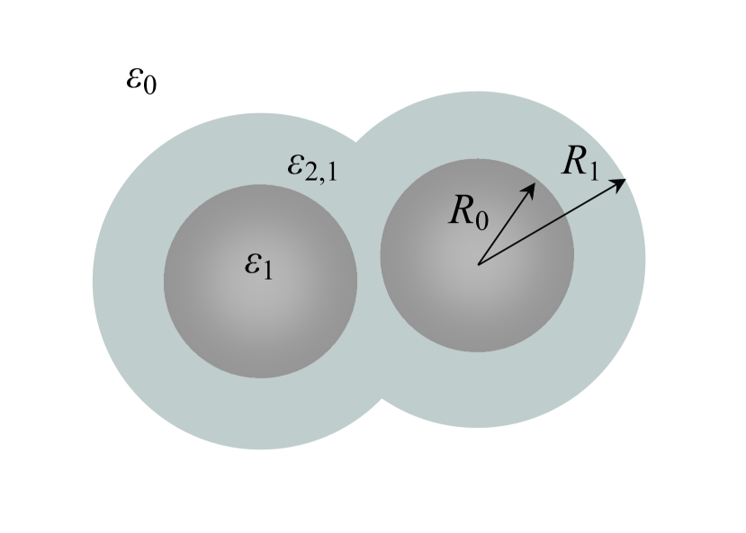
(a)

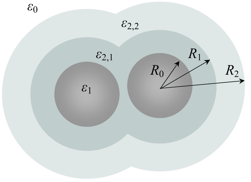
(b)

Figure 1: A composite electrolyte viewed as a dispersion of filler particles, with hard cores and penetrable interphase layers, embedded into a uniform matrix. The cases of one-shell (homogeneous, a) and two-shell (inhomogeneous, b) layers are shown.

To complete the model, a rule defining the complex permittivity distribution $\hat{\varepsilon}=\hat{\varepsilon}({\bf{r}})$ in the dispersion is needed. We assume that the local properties of the dispersion are formed according to the principle of dominance: if some of its constituents overlap, the properties of the dominant one are expressed to the exclusion of those of the others. The order of dominance is: hard cores $>$ penetrable shells with a smaller $j$ $>$ penetrable shells with a larger $j$ $>$ the matrix. Consequently, the local value $\hat{\varepsilon}({\bf{r}})$ is determined only by the distance $l\equiv\min\limits_{{\bf r}_{a}}|{\bf r}-{{\bf r}_{a}}|$ from the point of interest ${\bf r}$ to the center of the nearest particle (${{\bf r}_{a}}$ are the position vectors of the particles):

$$\hat{\varepsilon}({\bf r})=\begin{cases}\hat{\varepsilon}_{1}&{\text{if}}\quad\,\,l<R_{0}\\ \hat{\varepsilon}_{2,j}&{\text{if}}\quad R_{j-1}<l<R_{j}\,\,(1\leq j\leq M)\\ \hat{\varepsilon}_{0}&{\text{if}}\quad\,\,l>R_{M}\end{cases}$$ (5)

In view of the accepted rule, the volume concentrations of the constituents are found as follows. Let $\phi=\phi(c,\delta)$ be the effective volume concentration (the sum of the hard-core, $c$, and penetrable-layer, $\phi-c$, volume concentrations) of filler particles for the case of uniform one-shell layers; here $\delta=t/R_{0}$ is the relative thickness of such layers, of thickness $t=R_{1}-R_{0}$, with respect to $R_{0}$. Given $\phi(c,\delta)$ and under suggestion (5), the overall volume concentration of regions with permittivity $\hat{\varepsilon}_{2,j}$ is

$$\phi_{j}=\phi(c,\delta_{j})-\phi(c,\delta_{j-1})$$ (6)

where $\delta_{j}=(R_{j}-R_{0})/R_{0}$, $\phi(c,0)=c$.

Thus, provided the fluctuation effects are negligible, the dispersion can be considered as an aggregate of non-overlapping regions with permittivities $\hat{\varepsilon_{1}}$, $\hat{\varepsilon}_{2,j}$, $\hat{\varepsilon}_{0}$ and net volume concentrations $c$, $\phi_{j}$, $1-\phi(c,\delta_{M})$, respectively. Within the CGA, its effective permittivity $\hat{\varepsilon}_{\rm eff}$ is found as follows. Let $\Pi_{0}({\bf r})$, $\Pi_{1}({\bf r})$ and $\Pi_{2,j}({\bf r})$ be the characteristic functions of the entire sets of those regions (occupied by, respectively, the real matrix, hard cores and $j$-th shells) which form a compact group at point ${\bf r}$ in the pertinent auxiliary system. The permittivity distribution in this system is written in form (1) with $\hat{\varepsilon}_{\rm f}=\hat{\varepsilon}_{\rm eff}$ and, in view of Eq. (5),

$$\delta\hat{\varepsilon}({\bf r})=(\hat{\varepsilon}_{0}-\hat{\varepsilon}_{\rm eff})\Pi_{0}({\bf r})+(\hat{\varepsilon}_{1}-\hat{\varepsilon}_{\rm eff})\Pi_{1}({\bf r})+\sum\limits_{j=1}^{M}(\hat{\varepsilon}_{2,j}-\hat{\varepsilon}_{\rm eff})\Pi_{2,j}({\bf r})$$ (7)

Due to the orthogonality of $\Pi_{0}({\bf r})$, $\Pi_{1}({\bf r})$ and $\Pi_{2,j}({\bf r})$ to one another, the moments of $\delta\hat{\varepsilon}({\bf r})$ are calculated readily:

$${\langle{\mathop{\left({\delta\hat{\varepsilon}({\rm{\bf r}})}\right)^{s}}}}\rangle=\frac{1}{V}\int\limits_{V}{\mathop{\left({\delta\hat{\varepsilon}({\rm{\bf r}})}\right)^{s}}}d{\bf r}=(1-\phi(c,\delta_{M}))(\hat{\varepsilon}_{0}-\hat{\varepsilon}_{\rm eff})^{s}+c(\hat{\varepsilon}_{1}-\hat{\varepsilon}_{\rm eff})^{s}+\sum\limits_{j=1}^{M}\phi_{j}(\hat{\varepsilon}_{2,j}-\hat{\varepsilon}_{\rm eff})^{s}$$ (8)

Then Eqs. (2), (3), and (4) give the equation for $\hat{\varepsilon}_{\rm eff}$:

$$(1-\phi(c,\delta_{M}))\frac{\hat{\varepsilon}_{0}-\hat{\varepsilon}_{\rm eff}}{2\,\hat{\varepsilon}_{\rm eff}+\hat{\varepsilon}_{0}}+c\frac{\hat{\varepsilon}_{1}-\hat{\varepsilon}_{\rm eff}}{2\,\hat{\varepsilon}_{\rm eff}+\hat{\varepsilon}_{1}}+\sum\limits_{j=1}^{M}\phi_{j}\frac{\hat{\varepsilon}_{2,j}-\hat{\varepsilon}_{\rm eff}}{2\,\hat{\varepsilon}_{\rm eff}+\hat{\varepsilon}_{2,j}}=0$$ (9)

Whence the desired equation for $\sigma_{\rm eff}$ is obtained:

$$(1-\phi(c,\delta_{M}))\frac{\sigma_{0}-\sigma_{\rm eff}}{2\,\sigma_{\rm eff}+\sigma_{0}}+c\frac{\sigma_{1}-\sigma_{\rm eff}}{2\,\sigma_{\rm eff}+\sigma_{1}}+\sum\limits_{j=1}^{M}\phi_{j}\frac{\sigma_{2,j}-\sigma_{\rm eff}}{2\,\sigma_{\rm eff}+\sigma_{2,j}}=0$$ (10)

For the case of penetrable layers with piecewise-continuous conductivity profile $\sigma_{2}=\sigma_{2}(r)$ and finite thickness, that is, in the limit $M\to\infty$, $\delta_{M}$ fixed, Eq. (10) takes the form

$$(1-\phi(c,\delta_{M}))\frac{\sigma_{0}-\sigma_{\rm eff}}{2\,\sigma_{\rm eff}+\sigma_{0}}+c\frac{\sigma_{1}-\sigma_{\rm eff}}{2\,\sigma_{\rm eff}+\sigma_{1}}+\int\limits_{0}^{\delta_{M}}du\frac{\partial\phi(c,u)}{\partial u}\frac{\sigma_{2}(u)-\sigma_{\rm eff}}{2\,\sigma_{\rm eff}+\sigma_{2}(u)}=0$$ (11)

where the layer’s conductivity profile $\sigma_{2}(r)$ is expressed as a function $\sigma_{2}=\sigma_{2}(u)$ of the variable $u=(r-R_{0})/R_{0}$, the relative distance from a current point in the layer to the surface of the core.

In deriving Eqs. (9) and (10) in the above way, the fact of spherical symmetry of cores and layers is actually insignificant; as a consequence, these equations remain valid for macroscopically homogeneous and isotropic dispersions of nonspherical particles, with properly determined $c$ and $\phi_{j}$. For spherical hard-core–penetrable-shell, $\phi=\phi(c,\delta)$ can be estimated using the scaled-particle approximation [45, 46] ($\psi=(1+\delta)^{-3}$, $\phi_{t}=c/\psi$):

$$\phi(c,\delta) = 1-(1-c)\exp{\left[-\frac{(1-\psi)\phi_{t}}{1-c}\right]}$$ (12)

$$\times\exp{\left[-\frac{3c\phi_{t}}{2(1-c)^{3}}\left(2-3\psi^{1/3}+\psi-c\left(3\psi^{1/3}-6\psi^{2/3}+3\psi\right)\right)\right]}$$

This result is in a good agreement with Monte Carlo simulations [47, 48]. We use it in further applications of the theory.

3 Processing experimental data

3.1 Fitting procedures

To put the theory to the test, we first check the applicability of the $M$-shell and continuous-layer approximations to the description of the concentration dependence of $\sigma_{\rm eff}$. Then we use the three-shell approximation to describe the temperature behavior of $\sigma_{\rm eff}$. The procedures involved consist of the following three steps:

1. Fitting experimental data [2, 4] for $\sigma_{\rm eff}$ as a function of $c$ at a fixed temperature with Eq. (10) in order to determine the relative thicknesses $\delta_{j}$ and conductivities $x_{2,j}=\sigma_{2,j}/\sigma_{0}$ of the shells in the layer. For each electrolyte under study, the number of the shells is taken not to exceed three.

In other words, the one-, two- and three-shell approximations are exploited for $\sigma_{2}(r)$ at this step. Outside the hard core ($r>R_{0}$, $u>0$), the corresponding conductivity profiles $x(u)=\sigma(r)/\sigma_{0}$ for the local conductivity values $\sigma(r)$ are, respectively,

$$x(u)=x_{2,1}+(1-x_{2,1})\theta(u-\delta_{1}),\quad M=1$$ (13)

$$x(u)=x_{2,1}+(x_{2,2}-x_{2,1})\theta(u-\delta_{1})+(1-x_{2,2})\theta(u-\delta_{2}),\quad M=2$$ (14)

$$x(u)=x_{2,1}+(x_{2,2}-x_{2,1})\theta(u-\delta_{1})+(x_{2,3}-x_{2,2})\theta(u-\delta_{2})+(1-x_{2,3})\theta(u-\delta_{3}),\quad M=3$$ (15)

where $\theta(u)$ is the unit step-function.

If the values of $x_{2,j}$ (or some of them) differ considerably, then $\sigma_{2}(r)$ consists of several distinct parts. We assume that these parts account for different mechanisms (discussed in subsection 3.2) that are responsible for the formation of $\sigma_{\rm eff}$ and contribute most significantly to $\sigma_{\rm eff}$ in certain ranges of $c$. To estimate these ranges, we take into account the following facts: in the system of the $j$th shells, with inner radius $R_{j-1}$ and outer radius $R_{j}$, percolation paths start to form at the threshold concentration $c=c_{{\rm c},j}$ given by the condition $\phi(c_{{\rm c},j},\delta_{j})=1/3$ (see [41]); the greatest value of these shells’ contribution to $\sigma_{\rm eff}$ occurs at $c=c_{{\rm m},j}$ where their volume concentration $\phi_{j}$ has a maximum; the parameter $x_{2,j}$ governs whether this contribution increases ($x_{2,j}>x_{\rm eff}|_{c_{{\rm c},j}}$) or decreases ($x_{2,j}<x_{\rm eff}|_{c_{{\rm c},j}}$) with $c$ in the interval $(c_{{\rm c},j},c_{{\rm m},j})$.

Consequently, the behavior of $\sigma_{\rm eff}$ in the interval $(c_{{\rm c},M},c_{{\rm m},M})$ is governed by the outermost shells ($j=M$), with the largest inner and outer radii; $\sigma_{\rm eff}$ increases if $x_{2,M}>1$ and decreases if $x_{2,M}>1$. As $c$ is further increased, the $(M-1)$th shells, with smaller inner $R_{M-2}$ and outer $R_{M-1}$ radii, start to contribute; the role of the $M$th shells starts to diminish; and the behavior of $\sigma_{\rm eff}$ with $c$ becomes governed by $x_{2,M-1}$. If, for instance, $x_{2,M-1}\gg x_{2,M}>1$, then $\sigma_{\rm eff}$ should keep growing with $c$. However, if $x_{2,M}>1$ and $x_{2,M-1}\ll x_{2,M}$, then a maximum of $\sigma_{\rm eff}$ is expected to appear near $c_{{\rm m},M}$; and if $x_{2,M}<1$ and $x_{2,M-1}\gg 1$, then a minimum of $\sigma_{\rm eff}$ is expected near $c_{{\rm m},M}$. For sufficiently large and differing $\delta_{M}$ and $\delta_{M-1}$, these local extrema may become resolvable. The parameters of their location and height (depth) are used to obtain preliminary estimates for $\delta_{M}$, $\delta_{M-1}$, and $x_{2,M}$; that for $x_{2,M-1}$ is obtained by varying $x_{2,M-1}$ so as to recover the behavior of $\sigma_{\rm eff}$ at $c>c_{{\rm m},M}$.

Similar considerations can be developed for other inner shells, should they be needed to incorporate a greater number of the mechanisms involved. They considerably restrict the ranges for admissible values of the fitting parameters. Furthermore, the shapes of fitting curves prove to be very sensitive to the fitting parameters’ variations. The result is that for the observed nonmonotonic dependences of $\sigma_{\rm eff}$ upon $c$, even by-hand fitting is efficient to obtain the fitting curves with reasonable percentage deviations, mostly within the interval $(-25\%,25\%)$, from experimental data and high values, $\approx 0.92$ to 0.99, for the coefficient of determination $R^{2}$. In the situation where the number of experimental points is limited and the experimental errors have not been reported, a further optimization of the fitting procedure for profiles (14) and (15) does not seem necessary.

2. Fitting the same data for $\sigma_{\rm eff}$ using Eq. (11) with $\sigma_{2}(r)$ generated by the continuously differentiable sigmoid-type functions ($0<u<\delta_{M}$)

$$x_{2}(u)=X_{21}+\frac{X_{22}-X_{21}}{1+\exp\left[-\frac{u-\Delta_{1}}{\alpha}\right]}+\frac{1-X_{22}}{1+\exp\left[-\frac{u-\Delta_{2}}{\alpha}\right]}$$ (16)

$$x_{2}(u)=X_{21}+\frac{X_{22}-X_{21}}{1+\exp\left[-\frac{u-\Delta_{1}}{\alpha}\right]}+\frac{X_{23}-X_{22}}{1+\exp\left[-\frac{u-\Delta_{2}}{\alpha}\right]}+\frac{1-X_{23}}{1+\exp\left[-\frac{u-\Delta_{3}}{\alpha}\right]}$$ (17)

In the limiting case $\alpha\to 0$ and $\delta_{M}\to\infty$, profiles (16) and (17) transform into profiles (14) and (15), respectively, with $\Delta_{j}=\delta_{j}$ and $X_{2,j}=x_{2,j}$ having the previous physical meanings. For $\alpha\neq 0$, $\Delta_{j}$ and $X_{2,j}$ should be viewed only as formal parameters in the generating functions (16) and (17).

At this step, the continuous-layer approximation is used in order to fit the experimental $\sigma_{\rm eff}$ versus $c$ data. In doing so, the layer’s conductivity profiles of types (16) and (17) are varied by increasing $\alpha$ as much as possible and adjusting $\Delta_{j}$ and $X_{2,j}$ properly.

3. Applying the three-shell approximation, with corresponding $\delta_{j}$ taken to be temperature-independent, to $\sigma_{\rm eff}$ versus $c$ data [4] for three conductivity isotherms of blends of amorphous OMPEO with PAAM in order to obtain the values for $\sigma_{2,j}$ and $\sigma_{0}$ at three different temperatures. Next, assuming that the latter conductivities obey the VTF equation

$$\sigma=\frac{A}{\sqrt{T}}\exp{\left(-\frac{B}{T-T_{0}}\right)}$$ (18)

the parameters $A$, $B$, and $T_{0}$ for each shell and the matrix are found by solving the pertinent systems of three equations. Finally, having $\delta_{j}$ from the same fitting procedure, and disregarding the temperature dependence of $\sigma_{1}$, the temperature dependence of $\sigma_{\rm eff}$ is recovered with Eq. (10) and contrasted with experiment.

3.2 Concentration dependence of $\sigma_{\rm eff}$

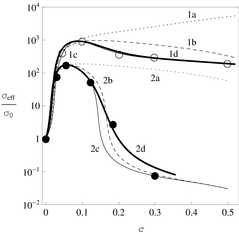
(a)

(b)

Figure 2: (a) Experimental data for $\sigma_{\rm eff}$ as a function of $c$ for PEO–NaI–NASICON [2] ($\circ$) and (PEO)₁₀–NaI–$\theta$-Al₂O₃ [4] ($\bullet$) electrolytes, and their fits within the one-shell, two-shell, and continuous layer approximations. The legends identify the fits with parameters specified in Table 1. (b) The corresponding one-particle’s conductivity profiles used to model the mesoscopic structure of these electrolytes.

(a)

(b)

Figure 3: (a) Experimental data for $\sigma_{\rm eff}$ as a function of $c$ for PEO–PAAM–LiClO₄ [2, 4] ($\circ$) and OMPEO–PAAM–LiClO₄ [4] ($\bullet$) electrolytes, and their fits within the two-shell, three-shell, and continuous layer approximations. The legends identify the fits with parameters specified in Table 1. (b) The corresponding one-particle’s conductivity profiles used to model the mesoscopic structure of these electrolytes.

Table 1: Parameters used to fit $\sigma_{\rm eff}$ vs $c$ data [2, 4] for composite polyether-based electrolytes at $t=25\,\rm{{}^{o}C}$ within several-shell and continuous-layer approximations, and $R^{2}$ values for appropriate fits.

Layer	La	$\sigma_{0}$, S/cm	$x_{1}$	$\delta_{1}$b	$\delta_{2}$b	$\delta_{3}$b	$x_{21}$b	$x_{22}$b	$x_{23}$b	$R^{2}$, %
				$\Delta_{1}$c	$\Delta_{2}$c	$\Delta_{3}$c	$X_{21}{\textsuperscript{c}}$	$X_{22}$c	$X_{23}{\textsuperscript{c}}$
PEO–NaI–NASICON
one-shell	1a	$9.86\times 10^{-9}$	$1.4\times 10^{4}$	1.6	–	–	1000	–	–	–
one-shell	1b		1.4	1.6	–	–	1300	–	–	–
two-shell	1c		70	1.0	1.55	–	400	20000	–	99.4
continuous,	1d		70	1.0	1.55	–	400	6000	–	95.5
$\alpha=0.05$
(PEO)10–NaI–$\theta$-Al2O3
one-shell	2a	$1.54\times 10^{-8}$	$6.5\times 10^{-13}$	2.1	–	–	230	–	–	–
two-shell	2b			0.7	2.1	–	0.12	435	–	92.8
two-shell	2c			0.8	2.1	–	0.12	520	–	98.6
continuous,	2d			0.9	2.1	–	0.12	560	–	95.0
$\alpha=0.05$
PEO–PAAM–LiClO4
two-shell	3a	$6.12\times 10^{-7}$	$1.6\times 10^{-6}$	0.15	0.60	–	5.0	800	–	88.7
three-shell	3b			0.16	0.50	0.80	5.0	1800	27	92.3
continuous,	3c			0.32	0.45	0.48	2.0	9400	27	92.9
$\alpha=0.03$
OMPEO–PAAM–LiClO4, after annealing
two-shell	4a	$1.61\times 10^{-5}$	$6.2\times 10^{-8}$	0.36	0.75	–	0.60	75	–	46.3
three-shell	4b			0.40	0.80	1.40	0.57	750	0.10	93.8
continuous,	4c			0.54	0.64	1.53	0.44	14200	0.10	81.7
$\alpha=0.02$

• Legends used to identify the corresponding fitting curves.

• Parameters for several-shell approximations.

• Parameters for continuous-layer approximations.

Figure 4: Percentage deviations of experimental $\sigma_{\rm eff}$ vs $c$ data for PEO–NaI–NASICON [2], (PEO)₁₀–NaI–$\theta$-Al₂O₃ [4], PEO–PAAM–LiClO₄ [2, 4], and OMPEO–PAAM–LiClO₄ [4] electrolytes from fitting curves 1c ($\square$), 2c ($\triangle$), 3b ($\triangledown$), and 4b ($\lozenge$), respectively (see Figs. 2 and 3). The filled markers: the same for fitting curves 1d, 2d, 3c, and 4c, respectively. The percentage deviation, $\approx 1040\,\%$, for the reported experimental point $c\approx 0.18$, $x_{\rm eff}\approx 2.8$ for (PEO)₁₀–NaI–$\theta$-Al₂O₃ (the fifth $\bullet$ in Fig. 2) from the 2c curve is not shown. The $R^{2}$ values for the above fits are summarized in Table 1.

Figure 5: Comparison of the three-shell approximation (solid lines 3b and 4b, see Table 1) with effective medium theory [4] (dashed lines, see Table 7 and Fig. 10 in [4]), both applied to experimental data [4] for PEO–PAAM–LiClO₄ ($\circ$) and OMPEO–PAAM–LiClO₄ (after annealing) ($\bullet$) at $25{\rm{}^{o}C}$ (concentration of LiClO₄ is equal to 10 mol % with respect to ether oxygen concentration).

Experimental data [2, 4] for several types of PEO- and OMPEO-based CPEs reveal a nonmonotonic behavior of $\sigma_{\rm eff}$ with $c$, with a maximum of $\sigma_{\rm eff}$ occurring for $c$ in between 0.05 and 0.1 for PEO–NaI–NASICON and (PEO)₁₀–NaI–$\theta$-Al₂O₃ (see Fig. 2(a)), that in between 0.2 and 0.3 for PEO–PAAM–LiClO₄ and OMPEO–PAAM–LiClO₄ (Fig. 3(a)), and possibly a minimum of $\sigma_{\rm eff}$ at $c$ close to 0.1 for OMPEO–PAAM–LiClO₄. Our fitting results (see Figs. 2(a), 3(a) and Table 1) for different types of $\sigma_{2}(r)$ (Figs. 2(b) and 3(b), respectively) give a clear hint at the inhomogeneity of it: a good agreement of our theory with data [2, 4] (see Fig. 4 for the percentage deviations of experimental data from our fits and Table 1 for the corresponding values of $R^{2}$) is reached within the two-shell approximation for CPEs with inorganic conductive (NASICON) or nonconductive ($\rm\theta$-Al₂O₃) filler particles, and the three-shell approximation for blends, complexed with LiClO₄, of PEO or OMPEO with PAAM. The values of $\delta_{j}$ and $x_{2,j}$ obtained correlate well with those expected to lead to the previously predicted scenarios of the behavior of $\sigma_{\rm eff}$ with $c$.

The use of the continuous-layer approximation, which may seem more adequate physically, alters the model shapes of the one-particle’s conductivity profiles noticeably; in fact, they become similar to those suggested in simulations [16, 35, 36]. However, at least for the indicated CPEs, this approximation does not change much the theoretical estimates for $\sigma_{\rm eff}$ as compared to those given by the three-shell approximation, yet usually reducing the $R^{2}$ values for the corresponding fits to the experiment. This fact gives grounds to apply the three-shell approximation to the study of the temperature behavior of $\sigma_{\rm eff}$ (see subsection 3.3). In a more comprehensive sense, it sustains the idea that $\sigma_{2}(r)$ effectively accounts for the net effect on $\sigma_{\rm eff}$ by different mechanisms.

Based on the conductivity values obtained (see Table 1), we can assume that $\sigma_{\rm eff}$ of the above CPEs is contributed by several common mechanisms [16]:

1. The amorphization of the polymer matrix by filler grains, that is, formation of a highly conductive (due to its large disorder and enhanced ionic mobility) amorphous polymer phase near the polymer-filler interface. This effect is attributed to the inhibition of the polymer crystallization process near the filler grains, which act as both nucleation centers for the polymer matrix and mechanical hindrances for polymer crystallite growth.

2. The stiffening effect of the filler on the amorphous phase, that is, the reduction of the flexibility of polymer chain segments and, consequently, of the ionic mobility in the close vicinity of the polymer-filler interface. It leads to a decrease in the local conductivity values ($\sigma_{2,1}$) there in comparison with those ($\sigma_{2,2}$) at greater distances from the interface. The innermost shell, of conductivity $\sigma_{2,1}$, is also supposed to incorporate the effects caused by irregularities in the shape of the filler grains (such as PAAM globes in polymer blends).

3. An effective decrease, compared to that of the pure filler, of the conductivity of highly-conductive filler grains inside CPEs caused by the formation of the highly-resistive polymer-filler interface. Our processing results for $\sigma_{1}$ in PEO–NaI–NASICON electrolytes agree with this expectation.

Of interest is the fact that the layer’s conductivity profiles inferred for the OMPEO-based electrolytes exhibit a peak followed by a trough, whereas those for the PEO-based electrolytes exhibit a peak alone (see Figs. 2(b) and 3(b)). To explain it, we should return to the concept of penetrable layers and emphasize that their conductivity profiles are not equivalent to the actual conductivity distributions around the hard cores, but represent a convenient way for modeling the effective microstructure of CPEs. The electrical properties of the layer’s outermost part determine the behavior of $\sigma_{\rm eff}$ at low $c$ where $\sigma_{\rm eff}$ is significantly contributed by the matrix. If the pure matrix polymer is relatively high-conductive (such as amorphous OMPEO compared to semicrystalline PEO), then the addition of a low-conductive polymer (such as PAAM) to it may detectably decrease its conductivity (say, due to the formation of complexes involving the ${\rm Li^{+}}$ cations and PAAM). A visible trough may then be needed on $\sigma_{2}(r)$ to incorporate this effect within our approach. As $c$ is increased, the interphase amorphous regions with higher conductivities come into play.

Finally, two examples of contrasting our results with those predicted by theory [4] (outlined in section 1) are given in Fig. 5. They clearly demonstrate that our approach exhibits a greater flexibility in the quantitative description of the electrical conductivities of CPEs.

3.3 Temperature dependence of $\sigma_{\rm eff}$

Figure 6: Experimental data [4] for the $t=0{\rm{}^{o}C}$ ($\circ$), $25{\rm{}^{o}C}$ ($\bullet$), and $100{\rm{}^{o}C}$ ($\nabla$) isotherms of $\sigma_{\rm eff}$ of OMPEO–PAAM–LiClO₄ electrolytes (with 10 mol% LiClO₄, after annealing) versus PAAM concentration. Dashed lines: VTF-type fits [4] with parameter values from Table 5 in [4]. Solid lines: our fits within the three-shell approximation, given by Eq. (10) at $M=3$ [see also Eqs. (11) and (15)], with parameter values summarized in Table 2. The percentage deviations of these data from and $R^{2}$ values for our fits are presented in Fig. 7.

Figure 7: Percentage deviations of experimental $\sigma_{\rm eff}$ vs $c$ data [4] for three $\sigma_{\rm eff}$ isotherms of OMPEO–PAAM–LiClO₄ electrolytes (with 10 mol% LiClO₄, after annealing) from our fits shown in Fig. 6. The markers $\circ$, $\bullet$, and $\nabla$ refer to the same data as those in Fig. 6. The $R^{2}$ values for these fits are 87.2, 91.4, and 94.5 %, respectively.

The results of applying the three-shell approximation to three $\sigma_{\rm{eff}}$ vs $c$ isotherms [4] of OMPEO–PAAM–LiClO₄ electrolytes (with 10 mol% LiClO₄, after annealing) are presented in Figs. 6, 7 and Table 2; the temperature-independent values $\delta_{1}=0.40$, $\delta_{2}$=0.80, and $\delta_{3}=1.40$ were used (see Table 1). The fitting values obtained for $\sigma_{0}$ and $\sigma_{2,j}$ were then used to estimate the VTF parameters for the CPE’s constituents; they are summarized in Table 3. Finally, employing Eqs. (10) at $M=3$ and (18) and the above geometrical and electrical data for the CPE’s constituents, the $\sigma_{\rm{eff}}$ vs $T$ dependences were recovered for all OMPEO–PAAM–LiClO₄ samples discussed in [4]; these results are shown in Figs. 8 and 9.

Three remarks are worth making here:

1. Our estimates $B=1270\,\rm{K}$ and $T_{0}=190\,\rm{K}$ for pure OMPEO turn out to be close to estimates $B=1200\,\rm{K}$ and $T_{0}=195\,\rm{K}$ obtained from direct conductivity measurements [4]. In contrast, our estimate for the preexponential factor $A$ differs noticeably from that in [4]: $A=36.1$ and $27.0\,\rm{S}\cdot\rm{K}^{1/2}/\rm{cm}$, respectively. Together with the fact that our theoretical curves fit the experimental data better, this result may indicate that the effective electrical properties of the polymer matrix are altered in the course of CPE preparation.

2. All our estimates of the VTF parameters for the shells fall in the value ranges reported in [4] for all OMPEO–PAAM–LiClO₄ samples studied. Therefore, from this point of view, they are not contradictory.

3. Taking into account the original uncertainties in the shells’ conductivity values obtained by processing the three conductivity isotherms, it can be concluded that the experimental data for the samples with 5, 25, and 40 vol% PAAM are reproduced by our theory well. Those for the samples with 10 and 50 vol% PAAM are recovered sufficiently well; the agreement is improved by a multiplicative renormalization (multiplication by a constant factor) of the theoretical results. The latter fact may be attributed to the discrepancy in the $A$-values obtained in [4] and in the present work for the matrix conductivity.

Table 2: Conductivity values, in S/cm, used to fit $\sigma_{\rm{eff}}$ vs $c$ isotherms [4] for OMPEO–PAAM–LiClO₄ electrolytes ^a,b (see Fig. 6).

Constituent	$t=0\,\rm{{}^{o}C}$	$t=25\,\rm{{}^{o}C}$	$t=100\,\rm{{}^{o}C}$
Matrix, $\sigma_{0}$	$4.64\times 10^{-7}$	$1.57\times 10^{-5}$	$1.78\times 10^{-3}$
First shell, $\sigma_{21}$	$5.75\times 10^{-7}$	$8.70\times 10^{-6}$	$4.21\times 10^{-4}$
Second shell, $\sigma_{22}$	$1.025\times 10^{-3}$	$7.74\times 10^{-3}$	$1.00\times 10^{-1}$
Third shell, $\sigma_{23}$	$1.07\times 10^{-7}$	$3.12\times 10^{-6}$	$1.36\times 10^{-4}$

• With 10 mol% LiClO₄.

• Due to the complexation of $\rm{Li}^{+}$ cations with PAAM chains, PAAM–LiClO₄ cores are essentially nonconductive, with room temperature conductivity $\sigma_{1}\sim 1\times 10^{-12}\,\rm{S/cm}$ [4]. This value was used in our calculations. An increase of $\sigma_{1}$ by several orders of magnitude does not affect, within the required accuracy, the results obtained.

Table 3: VTF parameters obtained for OMPEO–PAAM–LiClO₄ electrolytes ^a

Constituent	$A$, $\rm{S}\times\rm{K}^{1/2}/\rm{cm}$	$B$, K	$T_{0}$, K
Matrix, $\sigma_{0}$	36.1a	1270	190
First shell, $\sigma_{21}$	4.33	1210	180
Second shell, $\sigma_{22}$	71.1	634	197
Third shell, $\sigma_{23}$	0.229	720	212

• With 10 mol% LiClO₄.

(a) (b)

Figure 8: Experimental data [4] for $\sigma_{\rm eff}$ as a function of temperature for OMPEO–PAAM–LiClO₄ electrolytes (10 mol% LiClO₄, after annealing) with 5 ($\nabla$), 10 ($\circ$), 25 ($\square$), 40 ($\blacktriangle$), and 50 ($\bullet$) vol% PAAM. Dashed lines, (b): VTF-type fits, with parameter values from Table 5 in [4], proposed by the authors of [4] for the same electrolytes with 10 and 50 vol% PAAM. Solid lines: our calculation results within the three-shell approximation, given by Eq. (10) at $M=3$, under the suggestion that the conductivities of the constituents obey the VTF equation (18) with parameter values summarized in Table 3. Dotted lines, (b): the same, but for multiplicatively renormalized $\sigma_{\rm eff}$: $0.40\,\sigma_{\rm eff}$ and $0.75\,\sigma_{\rm eff}$ for electrolytes with 10 and 50 vol% PAAM, respectively. The percentage deviations of the above data from and $R^{2}$ values for the calculated (and, if so, renormalized) curves are presented in Fig. 9.

Figure 9: Percentage deviations of experimental $\sigma_{\rm eff}$ vs $T$ data [4] for OMPEO–PAAM–LiClO₄ electrolytes (10 mol% LiClO₄, after annealing) from the calculated (and, if so, renormalized) curves in Fig. 8. The deviations are calculated for all the electrolyte samples with 5 ($\nabla$), 10 ($\circ$), 25 ($\square$), 40 ($\blacktriangle$), and 50 ($\bullet$) vol% PAAM. The $R^{2}$ values for the indicated curves are 94.8, 94.0, 83.4, 77.5, and 96.0 %, respectively.

4 Conclusion

We have proposed a new approach to finding the effective quasistatic electrical conductivity $\sigma_{\rm eff}$ of CPEs. Its two major features are as follows:

1. The microstructure of a CPE is viewed as a result of embedding hard-core particles with adjacent penetrable (freely overlapping) layers into a uniform matrix. The layers are isotropic and, in general, inhomogeneous: they comprise a finite or infinite number of concentric shells. With the order of dominance taken to be hard cores $>$ shorter-radius shells $>$ longer-radius shell $>$ the matrix, the local value of the complex permittivity and, consequently, that of the quasistatic electrical conductivity in the system are determined by the distance from the point of interest to the center of the nearest particle. The layer’s conductivity profile is expected to account for different mechanisms contributing to the electrical properties of real CPEs. Some of its parts should have enhanced ionic conductivity, as compared to that of the polymer-based matrix with a higher degree of crystallinity, to form percolation paths.

2. The effective complex permittivity and then $\sigma_{\rm eff}$ are found for the model by applying the CGA. This approach makes it possible to avoid a detailed modeling of the many-particle polarization and correlation process in the system. The desired $\sigma_{\rm eff}$ is eventually shown to satisfy an integral relation found by summing up all the moments of the local complex permittivity deviations from the effective complex permittivity and passing to the quasistatic limit.

Putting the model to the test reveals that it is capable of recovering extensive experimental data [2, 4] for a series of PEO- and OMPEO-based electrolytes in a wide range of concentration. However, the agreement between the theory and experiment is reachable only under the suggestion of electrical inhomogeneity of the layers. To reproduce the major features of the concentration behavior of $\sigma_{\rm eff}$ for those data, the two-shell structures for $\sigma_{2}(r)$ are sufficient to be used for PEO–NaI–NASICON  [2] and (PEO)₁₀–NaI–$\theta$-Al₂O₃ [4]), and the three-shell ones for PEO–PAAM–LiClO₄ [2, 4] and OMPEO–PAAM–LiClO₄ [4]. The continuous sigmoid-type analogues of these conductivity profiles are also proposed. Their shapes are similar to those suggested in simulations [16, 35, 36]. Finally, finding the VTF parameters for the polymer matrix and shell conductivities obtained by processing the three available conductivity isotherms within the three-shell approximation, the temperature behavior of $\sigma_{\rm eff}$ for different samples of OMPEO–PAAM–LiClO₄ [4] is recovered satisfactorily.

The fitting results indicate that for the above CPEs, the observed behavior of $\sigma_{\rm eff}$ can be attributed to several mechanisms: (1) a change of the matrix’s conductivity in the course of preparation of a CPE; (2) an amorphization of the polymer matrix by filler grains; (3) a stiffening effect of the filler grains on the amorphous phase; (4) effects caused by irregularities in the filler grains’ shapes; (5) a formation of a highly-resistive polymer-filler interface. These mechanisms are effectively taken into account through the parameters of the outermost [mechanism (1)], central [mechanism (2)], and innermost [mechanisms (3) and (4)] parts in $\sigma_{2}(r)$, which gradually come into play as $c$ is increased; or a reduced value, compared to that in a solitary state, of the conductivity for highly-conductive filler grains inside CPEs [mechanism (5)].

References

- [1] J. Płocharski, W. Wieczorek, PEO based composite solid electrolyte containing NASICON, Solid State Ionics 28–30 (1988) 979–982. doi:10.1016/0167-2738(88)90315-3.
- [2] J. Przyluski, M. Siekierski, W. Wieczorek, Effective medium theory in studies of conductivity of composite polymeric electrolytes, Electrochimica Acta 40 (1995) 2101–2108. doi:10.1016/0013-4686(95)00147-7.
- [3] W. Wieczorek, K. Such, H. Wyciślik, J. Płocharski, Modifications of crystalline structure of PEO polymer electrolytes with ceramic additives, Solid State Ionics 36 (1989) 255–257. doi:10.1016/0167-2738(89)90185-9.
- [4] W. Wieczorek, K. Such, Z. Florjanczyk, J. Stevens, Polyether, polyacrylamide, composite electrolytes with enhanced conductivity, J. Phys. Chem. 98 (1994) 6840–6850. doi:10.1021/j100078a029.
- [5] M. A. Moharram, M. A. Soliman, H. M. El-Gendy, Electrical conductivity of poly(acrylic acid) – polyacrylamide complexes, J. Appl. Polymer Sci. 68 (1998) 2049–2055. doi:10.1002/(SICI)1097-4628(19980620)68:12¡2049::AID-APP19¿3.0.CO;2-W.
- [6] A. Zalewska, W. Wieczorek, J. R. Stevens, Composite polymeric electrolytes from the system, J. Phys. Chem. 100 (1996) 11382–11388. doi:10.1021/jp952909n.
- [7] M. Siekierski, K. Nadara, Mesoscale models of AC conductivity in composite polymeric electrolytes, J. Pow. Sour. 173 (2007) 748–754. doi:10.1016/j.jpowsour.2007.05.063.
- [8] J. R. MacCallum, C. Vincent (Eds.), Polymer Electrolyte Reviews, vol. 1, 1987 and vol. 2, 1989, Elsevier Applied Science, London.
- [9] B. Scrosati (Ed.), Applications of Electroactive Polymers, Chapman & Hall, London, 1993.
- [10] P. Bruce (Ed.), Solid State Electrochemistry, Cambridge University Press, Cambridge, 1995.
- [11] E. Quartarone, P. Mustarelli, A. Magistris, PEO-based composite polymer electrolytes, Solid State Ionics 110 (1998) 1–14. doi:10.1016/S0167-2738(98)00114-3.
- [12] J. Y. Song, Y. Y. Wang, C. Wan, Review of gel-type polymer electrolytes for lithium-ion batteries, J. Pow. Sour. 77 (1999) 183–197. doi:10.1016/S0378-7753(98)00193-1.
- [13] F. Croce, L. Persi, F. Ronci, B. Scrosati, Nanocomposite polymer electrolytes and their impact on the lithium battery technology, Solid State Ionics 135 (2000) 47–52. doi:10.1016/S0167-2738(00)00329-5.
- [14] C. Sequeira, D. Santos (Eds.), Polymer Electrolytes. Fundamentals and Applications, Woodhead Publishing, Oxford, 2010.
- [15] J.-M. Tarascon, P. Simon, Electrochemical Energy Storage, Vol. 1, ISTE and John Wiley & Sons, 2015.
- [16] W. Wieczorek, M. Siekierski, Nanocomposites. Ionic Conducting Materials and Structural Spectroscopies, Springer, New York, 2008, Ch. Composite Polymeric Electrolytes, pp. 1–70.
- [17] J. Przyłuski, et al., Proton conducting polymeric electrolytes from poly (ethyleneoxide) system, in: B. V. R. Chowdari, Q. Liu, L. Chen (Eds.), Recent Advances in Fast Ion Conducting Materials and Devices. Proc. 2nd Asian Conference on Solid State lonics, World Scientific, Singapore, 1990, p. 307.
- [18] L. A. Bulavin, I. A. Melnyk, A. I. Goncharuk, V. V. Klepko, N. I. Lebovka, E. A. Lysenkov, Effect of molecular weight on the properties of polyethylene glycol doped by multiwalled carbon nanotubes, Dopov. Nac. akad. nauk Ukr. 8 (2015) 72–78.
- [19] F. Croce, B. Scrosati, M. G., Electrochemical and spectroscopic study of the transport properties of composite polymer electrolytes, Chem. Mater. 4 (1992) 1134–1136. doi:10.1021/cm00024a003.
- [20] J. Płocharski, W. Wieczorek, J. Przyłuski, K. Such, Mixed solid electrolytes based on poly(ethylene oxide), Appl. Phys. A 49 (1989) 55–60. doi:10.1007/BF00615464.
- [21] J. Przyłuski, K. Such, H. Wyciślik, W. Wieczorek, Z. Floriańczyk, PEO–based polymer blends as materials for solid electrolytes, Synth. Met. 35 (1989) 241–247. doi:10.1016/0379-6779(90)90048-P.
- [22] C.-W. Nan, Physics of inhomogeneous inorganic materials, Prog. Mater. Sci. 37 (1993) 1–116. doi:10.1016/0079-6425(93)90004-5.
- [23] S. Jiang, J. B. Wagner, A theoretical model for composite electrolytes – I. Space charge layer as a cause for charge–carrier enhancement, J. Phys. Chem. Solids 56 (1995) 1101–1111. doi:10.1016/0022-3697(95)00025-9.
- [24] S. Jiang, J. B. Wagner, A theoretical model for composite electrolytes – II. Percolation model for ionic conductivity enhancement, J. Phys. Chem. Solids. 56 (1995) 1113–1124. doi:10.1016/0022-3697(95)00026-7.
- [25] M. G. Todd, F. G. Shi, Characterizing the interphase dielectric constant of polymer composite materials: Effect of chemical coupling agents, J. Appl. Phys. 94 (2003) 4551–4557. doi:10.1063/1.1604961.
- [26] J. C. Maxwell, A Treatise on Electricity and Magnetism, 1st Edition, Vol. 1, Clarendon Press, Oxford, 1873, pp. 362–365.
- [27] J. C. M. Garnett, Colours in metal glasses and metalic films, Trans. R. Soc. Lond. A 203 (1904) 385. doi:10.1098/rsta.1904.0024.
- [28] L. D. Landau, E. M. Lifshitz, L. P. Pitaevskii, Course of Theoretical Physics. Electrodynamics of Continuous Media, Vol. 8, Pergamon, Oxford, 1984.
- [29] D. Bruggeman, Berechnnung verschiedener physikalischer konstanten von heterogenen substanzen 1. dielektrizitätskonstanten und leitfähigkeiten der mischkörper aus isotropen substanzen, Ann. Phys. (Leipzig) 24 (1935) 636–664. doi:10.1002/andp.19354160705.
- [30] R. Landauer, The electrical resistance of binary metallic mixtures, J. Appl. Phys. 23 (1952) 779. doi:10.1063/1.1702301.
- [31] M. Nakamura, A method to improve the effective medium theory towards percolation problem, J. Phys. C: Solid State Phys. 15 (1982) L749–752. doi:10.1088/0022-3719/15/23/005.
- [32] M. Nakamura, Conductivity for the site-percolation problem by an improved effective-medium theory, Phys. Rev. B 29 (1984) 3691–3693. doi:10.1103/PhysRevB.29.3691.
- [33] C.-W. Nan, D. M. Smith, On comment on “Enhancement of ionic conduction in CaF2 and BaF2 by dispersion of Al2O3”, J. Mat. Sci. Lett. 10 (1991) 1142–1143. doi:10.1007/BF00744107.
- [34] C.-W. Nan, D. M. Smith, A.c. electrical properties of composite solid electrolytes, Mat. Sci. Eng. B 10 (1991) 99–106. doi:10.1016/0921-5107(91)90115-C.
- [35] M. Siekierski, K. Nadara, Modeling of conductivity in composites with random resistor networks, Electrochimica Acta 50 (2005) 3796–3804. doi:10.1016/j.electacta.2005.02.046.
- [36] M. Siekierski, K. Nadara, P. Rzeszotarski, Conductivity simulation in composite polymeric electrolytes, J. New Mat. Electrochem. Systems 9 (2006) 375–390. doi:10.1.1.455.1852.
- [37] M. Y. Sushko, Dielectric permittivity of suspensions, Zh. Eksp. Teor. Fiz. 132 (2007) 478–484, [JETP 105 (2007) 426–431]. doi:10.1134/S106377610.
- [38] M. Y. Sushko, S. K. Kris’kiv, Compact group method in the theory of permittivity of heterogeneous systems, Zh. Tekh. Fiz. 79 (2009) 97–101, [Tech. Phys. 54 (2009) 423–427]. doi:10.1134/S1063784209030165.
- [39] M. Y. Sushko, Effective permittivity of mixtures of anisotropic particles, J. Phys. D: Appl. Phys. 42 (2009) 155410. doi:10.1088/0022-3727/42/15/155410.
- [40] M. Y. Sushko, Effective dielectric response of dispersions of graded particles, Phys. Rev. E 96 (2017) 062121. doi:10.1103/PhysRevE.96.062121.
- [41] M. Y. Sushko, A. K. Semenov, Conductivity and permittivity of dispersed systems with penetrable particle-host interphase, Cond. Matter Phys. 16 (2013) 13401. doi:10.5488/CMP.16.13401.
- [42] M. Y. Sushko, V. Y. Gotsulskiy, M. V. Stiranets, Finding the effective structure parameters for suspensions of nano-sized insulating particles from low-frequency impedance measurements, J. Mol. Liq. 222 (2016) 1051–1060. doi:10.1016/j.molliq.2016.07.021.
- [43] S. Tomylko, O. Yaroshchuk, N. Lebovka, Two-step electrical percolation in nematic liquid crystals filled with multiwalled carbon nanotubes, Phys. Rev. E 92 (2015) 012502. doi:10.1103/PhysRevE.92.012502.
- [44] A. K. Semenov, On applicability of differential mixing rules for statistically homogeneous and isotropic dispersions, J. Phys. Commun. 2 (2018) 035045. doi:10.1088/2399-6528/aab060.
- [45] P. A. Rikvold, G. Stell, Porosity and specific surface for interpenetrablesphere models of twophase random media, J. Chem. Phys. 82 (1985) 1014–1020. doi:10.1063/1.448966.
- [46] P. A. Rikvold, G. Stell, D-dimensional interpenetrable-sphere models of random two-phase media: Microstructure and an application to chromatography, J. Colloid Interface Sci. 108 (1985) 158–173. doi:10.1016/0021-9797(85)90246-2.
- [47] S. B. Lee, S. Torquato, Porosity for the penetrable-concentric-shell model of two-phase disordered media: Computer simulation results, J. Chem. Phys. 89 (1988) 3258–3263. doi:10.1063/1.454930.
- [48] M. Rottereau, J. C. Gimel, T. Nicolai, D. Durand, 3d Monte Carlo simulation of site-bond continuum percolation of spheres, Eur. Phys. J. E 11 (2003) 61–64. doi:10.1140/epje/i2003-10006-x.