Stiffness pathologies in discrete granular systems: bifurcation, neutral equilibrium, and instability in the presence of kinematic constraints

Abstract

The paper develops the stiffness relationship between the movements and forces among a system of discrete interacting grains. The approach is similar to that used in structural analysis, but the stiffness matrix of granular material is inherently non-symmetric because of the geometrics of particle interactions and of the frictional behavior of the contacts. Internal geometric constraints are imposed by the particles’ shapes, in particular, by the surface curvatures of the particles at their points of contact. Moreover, the stiffness relationship is incrementally non-linear, and even small assemblies require the analysis of multiple stiffness branches, with each branch region being a pointed convex cone in displacement-space. These aspects of the particle-level stiffness relationship gives rise to three types of micro-scale failure: neutral equilibrium, bifurcation and path instability, and instability of equilibrium. These three pathologies are defined in the context of four types of displacement constraints, which can be readily analyzed with certain generalized inverses. That is, instability and non-uniqueness are investigated in the presence of kinematic constraints. Bifurcation paths can be either stable or unstable, as determined with the Hill–Bažant–Petryk criterion. Examples of simple granular systems of three, sixteen, and sixty four disks are analyzed. With each system, multiple contacts were assumed to be at the friction limit. Even with these small systems, micro-scale failure is expressed in many different forms, with some systems having hundreds of micro-scale failure modes. The examples suggest that micro-scale failure is pervasive within granular materials, with particle arrangements being in a nearly continual state of instability.

1 Introduction

In the mid-2000s, several independent works were published on the nature of internal rigidity, uniqueness, and stability of discrete granular materials [1, 2, 3]. When violated, these favorable conditions give rise to failure, weakening, and localized deformation, conditions that we broadly designate as stiffness pathologies. The incremental macro-scale behavior of granular materials is known to be exceedingly complex, and the strength, stiffness, and various forms of failure (diffuse, localized, static, dynamic, etc.) at the continuum, macro-scale have received extensive investigation in the past decades. At the risk of making the nearly impenetrable and confounding behavior of these materials even more so, we return to a study of discrete failure — in its many forms — by addressing the internal particle-scale stiffness and rigidity of granular materials.

The works of Bagi [1], Nicot and Darve [3], and Kuhn and Chang [2], viewed granular materials at the micro-level, treating a material region, which might appear continuous at a larger scale, as a collection of discrete and notionally rigid granules that interact when touching each other at idealized contact points. The paper takes a similar primitive approach, departing from a continuum framework and treating a granular medium as a discrete system of interacting grains. As one difference between discrete and and continuous media, the discrete topology of a granular medium can be expressed as a multi-graph [4, 5] with a finite (or at most, countable) number of vertices (grains) and edges (contacts between grains), and we adopt this elemental view of a granular material. Because a discrete graph expresses the topology of a finite open set (e.g., a planar graph is homeomorphic with a sphere), a graph has no interior, and without an interior, it has no boundary, no unit normal on the boundary, no volume, and no surface area. Our vocabulary is instead of movement and force and of the relationship between them — stiffness. Movements and forces are associated with particles and contacts: the particle forces are external forces, and the contact forces are internal forces, but no distinction is made between boundary and interior forces, as there is no boundary or interior.

Another difference between discrete and continuous systems arises in the choice of a reference configuration of stable behavior. With continuous systems having simple boundaries, one can usually distinguish a “fundamental deformation” with which a buckled or bifurcated deformation can be compared (for example, the fundamental deformation of a persistently straight column or of a region that deforms in a fundamental, uniform mode without shear bands). Sliding between discrete particles at their contacts, a primary mechanism of deformation and failure, usually occurs in only a subset of the contacts, and predetermination of this sliding subset is usually quite difficult. As such, the fundamental deformation of a discrete granular system can rarely be presaged.

The paper extends the current understanding of discrete systems, by presenting a thorough accounting of four different types of geometric effects in granular media, for which three of the effects behave as internal follower forces. These geometric effects are a results of the internal geometric constraints that are imposed by the particles’ shapes, in particular, by the surface curvatures of the particles at their points of contact. The paper also describes four types of external displacement constraint, using the theory of generalized inverses to address three of the types. We also extend an accepted definition of stability by incorporating the internal geometric effects within granular systems and give a comprehensive accounting of three types of pathologic behaviors in discrete systems: neutral equilibrium, bifurcation and path instability, and instability of equilibrium, with Bažant–Petryk theory applied to the problem of path instability. This accounting is detailed for each of the four types of displacement constraints. An analysis of potential pathologies is particularly vexing with granular materials, as behavior is incrementally non-linear, and we present a systematic means of determining the consistency of a possible pathology with the assumed contact-level stiffness conditions. We also present examples of simple granular assemblies and show how the various pathologies arise in these systems.

The plan of the paper is as follows. In the next section, we develop essential elements for characterizing the stiffness of discrete systems. These elements include the derivation of the stiffness matrix of a granular assembly, including those stiffness components that depend upon the current forces and their geometric alteration (Section 2.2). A thermodynamic framework for analyzing the stability of a granular system is then developed in Section 2.3. In Section 2.4, we consider possible constraints placed upon a granular system by its surroundings, as these limitations will restrict the available modes of deformation and instability. Four categories of displacement constraints are developed in this section. To provide a specific framework for these principles, Section 2.5 describes a standard two-branch frictional model for the contact interaction between particles, and Section 2.6 places this model in the context of an entire assembly’s stiffness matrix.

After establishing these principles, we define various stiffness pathologies in Section 3 (controllability, bifurcation, and instability). Examples of several simple granular systems are then analyzed in Section 4. These examples are engaged using the methods and language of linear algebra, which we hope will clarify distinctions among the different pathologies.

With occasional exceptions, we use vector and matrix, rather than index, notation for most objects and operations. Vectors and matrices are enclosed in brackets when they contain information for an entire assembly; but brackets are usually excluded when the vector or matrix is referenced to a single contact. Vectors are written with bold lower case letters; matrices are with bold upper case letters; and scalars are normal lower case letters. Inner, outer, and dyad products are denoted as follows: inner products $\mathbf{x}\cdot\mathbf{y}=x_{i}y_{i}$ and $\mathbf{A}\cdot\mathbf{x}=A_{ij}x_{j}$; outer product $\mathbf{x}\times\mathbf{y}=e_{ijk}x_{j}y_{k}$; and dyad product $\mathbf{x}\otimes\mathbf{y}=x_{i}y_{j}$.

2 Stiffness framework for discrete systems

Bagi [1] and Kuhn and Chang [2], approached the discrete mechanics of granular materials from a structural mechanics perspective. These concurrent works developed a stiffness relationship between movement and force in matrix form, so that established concepts of stability, bifurcation, softening and controllability, already used in structural analysis, could also be applied to granular assemblies (see, for example, Bazant [6]). Both works were preceded by others that developed stiffness matrices for granular systems [7, 8, 9], but these earlier works neglected second-order geometric changes, which are essential to the developments that follow. A general stiffness relationship was also developed by Agnolin and Roux [10, 11], who had considered geometric effects in the appendices of these works. We will use the notation of Kuhn and Chang [2] as it makes useful distinctions between objective and non-objective quantities, which become relevant when distinguishing various stiffness pathologies.

2.1 Notation

The shapes, positions, orientations, contact forces, and loading history of the $N$ particles in a granular assembly are assumed known at time $t$, and we develop the conditions for equilibrium in a deformed state at $t+dt$. Each particle is assumed a hard body that interacts with neighboring particles at their shared compliant contacts. Movement and deformation are assumed slow and quasi-static, so that we can neglect viscous or gyroscopic forces. As shown in Fig. 1, a particle $p$ touches particle $q$ at a contact $c$, with $q$ being a member of the set $\mathcal{C}_{p}^{q}$ of $p$’s neighboring particles, $q\in\mathcal{C}_{p}^{q}$, and with $c$ being a member of the set $\mathcal{C}_{p}^{c}$ of $p$’s contacts, $c\in\mathcal{C}_{p}^{c}$.

In this work, an assembly’s contact topology is represented as a directed multi-graph (a multi-digraph). The graph is “multi”, because a pair of particles can share multiple contacts, as can occur with non-convex particles. The graph is “directed”, because we treat the $pq$ contact (from $p$ to $q$) as distinct from the contact $qp$ (from $q$ to $p$). This approach allows a more straightforward derivation and is consistent with the non-symmetry of the stiffness matrix, as we will see that the $pq$ stiffness can differ from the $qp$ stiffness. The system can also include isolated “rattler” particles that are not in contact with other particles. With this situation, we can adopt two different approaches. We can include these rattlers as isolated nodes of a complete topology, which will lead to numerous zero-stiffness modes of neutral equilibrium, or we can consider only the load-bearing network of contacting (non-rattler) particles and then update the topology whenever rattlers are freshly released from or incorporated into the network. For reasons given in Section 2.2, we take the latter approach and consider only the current load-bearing network of contacts and particles.

Vector $\mathbf{u}^{p}$ is the location of a material reference point $\chi^{p}$ attached to $p$; $\boldsymbol{\theta}^{p}$ are the orientation cosines of $p$; and $\mathbf{b}^{p}$ and $\mathbf{w}^{p}$ are the external force and moment that act upon $p$ at the point $\chi^{p}$.

Figure 1: Contact between particles $p$ and $q$: (a) geometry; and (b) forces.

The entire particle system has $M$ contacts. The single contact vector $\mathbf{r}^{c,p}$, is from $\chi^{p}$ to its contact $c$; $\mathbf{n}^{c}$ is the outward unit vector normal to the surface of $p$ at contact $c$; and $\mathbf{f}^{c}$ and $\mathbf{m}^{c}$ are the contact force and moment exerted upon $p$ at $c$.

Although the two particles, $p$ and $q$, can share multiple contacts $c$, we will use the more convenient notations $\mathbf{r}^{pq,p}$, $\mathbf{n}^{pq}$, $\mathbf{f}^{pq}$, and $\mathbf{m}^{pq}$ with the understanding that the pair $pq$ can represent one of several contacts $c$ between $p$ and $q$. With this notation, force $\mathbf{f}^{pq}$ and moment $\mathbf{m}^{pq}$ act upon particle $p$, and $\mathbf{n}^{pq}$ is directed outward from $p$. We must distinguish, however the two “$\mathbf{r}^{pq}$” contact vectors for contact $pq$: vector $\mathbf{r}^{pq,p}$ is directed from $p$ to the contact; whereas vector $\mathbf{r}^{pq,q}$ is directed from $q$ to the contact.

We gather the particle positions and orientations of all $N$ particles into a stacked column vector $[\mathbf{u}/\boldsymbol{\theta}]$, the external forces and moments into the stacked complementary vector $[\mathbf{b}/\mathbf{w}]$, and the internal contact forces and moments into the stacked vector $[\mathbf{f}/\mathbf{m}]$:

$$\left.\begin{array}[]{r}\mathbf{u}^{p}\\ \boldsymbol{\theta}^{p}\end{array}\right\}_{6\times 1}\;\rightsquigarrow\;\left[\begin{array}[]{@{\extracolsep{\fill}}c@{\extracolsep{\fill}}}\mathbf{u}\\ \hdashline[1pt/1pt]\boldsymbol{\theta}\end{array}\right]_{6N\times 1}\!,\quad\left.\begin{array}[]{r}\mathbf{b}^{p}\\ \mathbf{w}^{p}\end{array}\right\}_{6\times 1}\;\rightsquigarrow\;\left[\begin{array}[]{@{\extracolsep{\fill}}c@{\extracolsep{\fill}}}\mathbf{b}\\ \hdashline[1pt/1pt]\mathbf{w}\end{array}\right]_{6N\times 1},\quad\left.\begin{array}[]{r}\mathbf{f}^{pq}\\ \mathbf{m}^{pq}\end{array}\right\}_{6\times 1}\;\rightsquigarrow\;\left[\begin{array}[]{@{\extracolsep{\fill}}c@{\extracolsep{\fill}}}\mathbf{f}\\ \hdashline[1pt/1pt]\mathbf{m}\end{array}\right]_{2(6M)\times 1}$$ (1)

where the “$\rightsquigarrow$” represents a matrix assembly process that gathers the individual “$p$” and “$pq$” vectors into vectors for the entire assembly. In these equations, $N$ is the number of particles, with each particle involving 3-vectors for the position, orientation, external force, and external moment; whereas, $M$ is the number of contacts, each with a 3-vector of contact force and a 3-vector of contact moment. Recalling that the $pq$ and $qp$ contact variants are treated separately, the stacked vector $[\mathbf{f}/\mathbf{m}]$ has $2(6M)$ components. Although two-dimensional (2D) systems can be represented with smaller vectors and matrices, these objects for a 2D system can be readily extracted from the 3D counterparts. We will sometimes compress the notation, with $[\mathbf{x}]$ , $[\mathbf{p}]$, and $[\,\boldsymbol{\mathfrak{f}}\,]$ representing the configuration, loading, and internal force vectors:

$$\left[\mathbf{x}\right]_{6N\times 1}=\left[\begin{array}[]{@{\extracolsep{\fill}}c@{\extracolsep{\fill}}}\mathbf{u}\\ \hdashline[1pt/1pt]\boldsymbol{\theta}\end{array}\right]\;\text{, }\quad\left[\mathbf{p}\right]_{6N\times 1}=\left[\begin{array}[]{@{\extracolsep{\fill}}c@{\extracolsep{\fill}}}\mathbf{b}\\ \hdashline[1pt/1pt]\mathbf{w}\end{array}\right]\;\text{, and}\quad\left[\,\boldsymbol{\mathfrak{f}}\,\right]_{2(6M)\times 1}=\left[\begin{array}[]{@{\extracolsep{\fill}}c@{\extracolsep{\fill}}}\mathbf{f}\\ \hdashline[1pt/1pt]\mathbf{m}\end{array}\right]$$ (2)

Nicot et al. [12] considered the stability of non-conservative structural systems, in which the external loads $[\mathbf{b}/\mathbf{w}]$ depend upon the positions and orientations, $[\mathbf{u}]$ and $[\boldsymbol{\theta}]$, of material points $\chi$ within the system. In this general setting, the $6N$ elements of the force vector $[\mathbf{p}]$ are functions of the positions $[\mathbf{x}]$ and an $L$-list of loading parameters $\mathbf{q}$:

$$\left[\mathbf{p}\right]_{6N\times 1}=\left[\rule{0.0pt}{10.76385pt}\mathbf{p}\left(\rule{0.0pt}{9.47217pt}[\mathbf{x}]_{6N\times 1},[\mathbf{q}]_{L\times 1}\right)\right]_{6N\times 1}$$ (3)

These systems include those with external follower forces having directions and magnitudes that change as the system is deformed, such as the two-bar (i.e. two-particle) Ziegler column with tangential loading, analyzed in [13, 12] (Fig. 2a).

Figure 2: Position-dependent external forces: (a) follower load on Ziegler column [12]; and (b) membrane loads.

For this articulated column, the list $[\mathbf{q}]$ is simply the single magnitude of the follower force, but the directed force $\mathbf{b}$ will depend upon the rotations of the bars. With compliant loading machines, the forces exerted by the machinery on peripheral particles can also depend upon these particles’ positions and orientations. Another example is a granular assembly enclosed within a rubber membrane that presses against the the assembly’s peripheral particles with an external confining pressure $p$ (Fig. 2b). Such membranes are commonly modeled as flat pieces of “virtual membrane” that apply the pressure as discrete external forces to points $\chi$ within the peripheral particles. The magnitudes and directions of the membrane forces depend on the sizes and orientations of the pieces, which depend, in turn, upon the positions $\mathbf{u}$ and orientations $\boldsymbol{\theta}$ of the particle points and of the pressure $p$, which serves as the single loading parameter in list $[\mathbf{q}]$.

If the external forces $[\mathbf{b}]$ and $[\mathbf{w}]$ depend on the particles’ positions $[\mathbf{u}]$ and $[\boldsymbol{\theta}]$, as in Eq. (3), then the incremental forces will depend upon changes in these positions and upon the $L$ loading parameters,

$$\left[d\mathbf{p}\right]=\left[\partial\mathbf{p}/\partial\mathbf{x}\right]_{6N\times 6N}\left[d\mathbf{x}\right]\>+\>\left[\partial\mathbf{p}/\partial\mathbf{q}\right]_{6N\times L}\left[d\mathbf{q}\right]_{L\times 1}$$ (4)

where the final term $[\partial\mathbf{p}/\partial\mathbf{q}][d\mathbf{q}]$ gives the loading increments $[d\mathbf{p}]$ produced by increments in the $L$ loading parameters (e.g., increments in the confining pressure, increments in the applied platen loads, etc.). We designate the loading matrix $[\partial\mathbf{p}/\partial\mathbf{q}]$ as $[\mathbf{Q}]$, and we designate the last product in Eq. (4) as the incremental loading vector $[d\mathfrak{p}]$:

$$\left[\mathbf{Q}\right]_{6N\times L}=\left[\partial\mathbf{p}/\partial\mathbf{q}\right]\quad\text{and}\quad\left[d\mathfrak{p}\right]_{6N\times 1}=\left[\partial\mathbf{p}/\partial\mathbf{q}\right]\left[d\mathbf{q}\right]=\left[\mathbf{Q}\right]\left[d\mathbf{q}\right]$$ (5)

where $[d\mathfrak{p}]$ serves as a lower-dimensional subspace of the more general incremental loading vector $[d\mathbf{p}]=[d\mathbf{b}/d\mathbf{w}]$. The term $[\partial\mathbf{p}/\partial\mathbf{x}]$ in Eq. (4) is one of several geometric effects that we will consider.

2.2 Equilibrium in initial and displaced states

The nature of the external loads — whether dead loads or follower loads — is known to affect the stability of structural systems. More subtle, however, are the forces among the particles within a granular system, which also can act as internal follower forces, since the directions of the inter-particle forces can depend upon the positions and orientations of the particles, $[\mathbf{u}]$ and $[\boldsymbol{\theta}]$. To reveal this dependence, we analyze a system that is assumed in equilibrium in both its initial and displaced states — at times $t$ and $t+dt$. The initial equilibrium of a particle $p$ requires

$$-\sum_{\mathclap{c\in\mathcal{C}^{c}_{p}}}\mathbf{f}^{pq}=\mathbf{b}^{p},\qquad-\sum_{\mathclap{c\in\mathcal{C}^{c}_{p}}}\left(\mathbf{m}^{pq}+\mathbf{r}^{pq,p}\times\mathbf{f}^{pq}\right)=\mathbf{w}^{p}$$ (6)

in which both summations include all of $p$’s contacts $c$. Recall that $\mathbf{r}^{pq,p}$ is the contact vector of contact $pq$, from the reference point $\chi^{p}$ of $p$ to its contact with $q$. The equilibrium equations of all $N$ particles are gathered into the matrix relation

$$\left[\mathbf{A}\right]_{6N\times 2(6M)}\left[\begin{array}[]{@{\extracolsep{\fill}}c@{\extracolsep{\fill}}}\mathbf{f}\\ \hdashline[1pt/1pt]\mathbf{m}\end{array}\right]_{2(6M)\times 1}=\left[\begin{array}[]{@{\extracolsep{\fill}}c@{\extracolsep{\fill}}}\mathbf{b}\\ \hdashline[1pt/1pt]\mathbf{w}\end{array}\right]_{6N\times 1}\quad\text{or}\quad\left[\mathbf{A}\right]\left[\,\boldsymbol{\mathfrak{f}}\,\right]=\left[\mathbf{p}\right]$$ (7)

where $[\mathbf{A}]$ is the statics matrix. At $t+dt$, the new positions, orientations, and forces are the sums $\mathbf{u}^{p}+d\mathbf{u}^{p}$, $\mathbf{b}^{p}+d\mathbf{b}^{p}$, $\mathbf{x}^{p}+d\mathbf{x}^{p}$, $\mathbf{r}^{pq}+d\mathbf{r}^{pq}$, $\mathbf{f}^{pq}+d\mathbf{f}^{pq}$, etc. By substituting these sums in Eq. (6) and then subtracting Eq. (6), we find the incremental conditions for continued equilibrium:

$$-\sum_{\mathclap{c\in\mathcal{C}^{c}_{p}}}d\mathbf{f}^{pq}=d\mathbf{b}^{p},\qquad-\sum_{\mathclap{c\in\mathcal{C}^{c}_{p}}}\left(d\mathbf{m}^{pq}+\mathbf{r}^{pq,p}\times d\mathbf{f}^{pq}+d\mathbf{r}^{pq,p}\times\mathbf{f}^{pq}\right)=d\mathbf{w}^{p}$$ (8)

Note that the statics matrix $[\mathbf{A}]$ depends upon the positions and orientations of the particles and contacts, $[\mathbf{A}]=[\mathbf{A}(\mathbf{x})]$, and is altered by the movements $d\mathbf{x}$. With this understanding, Eq. (6) is equivalent to the differential of Eq. (7), when applied to all particles of the system:

$$\left[\rule{0.0pt}{9.47217pt}(\partial\mathbf{A}/\partial\mathbf{x})\cdot d\mathbf{x}\right]\left[\begin{array}[]{@{\extracolsep{\fill}}c@{\extracolsep{\fill}}}\mathbf{f}\\ \hdashline[1pt/1pt]\mathbf{m}\end{array}\right]+\left[\mathbf{A}\right]\left[\begin{array}[]{@{\extracolsep{\fill}}c@{\extracolsep{\fill}}}d\mathbf{f}\\ \hdashline[1pt/1pt]d\mathbf{m}\end{array}\right]=\left[\begin{array}[]{@{\extracolsep{\fill}}c@{\extracolsep{\fill}}}d\mathbf{b}\\ \hdashline[1pt/1pt]d\mathbf{w}\end{array}\right]\quad\text{or}\quad\left[\rule{0.0pt}{9.47217pt}(\partial\mathbf{A}/\partial\mathbf{x})\cdot d\mathbf{x}\right]\left[\,\boldsymbol{\mathfrak{f}}\,\right]+\left[\mathbf{A}\right]\left[\,d\boldsymbol{\mathfrak{f}}\,\right]=\left[d\mathbf{p}\right]$$ (9)

The first term on the left can be expressed with index notation as $A_{ij,k}dx_{k}\mathfrak{f}_{j}$, where $\mathfrak{f}_{j}$ is an element of vector $[\boldsymbol{\mathfrak{f}}]=[\mathbf{f}/\mathbf{m}]$. As was noted near the start of Section 2.1, a granular system can include non-contacting rattler particles, which can become incorporated in the the load-bearing network of particles during $dt$, even as some load-bearing particles become disengaged rattlers. If we choose to model the entire system of particles — both load-bearing and rattler — and allow all possible changes to the contact topology, then matrix $[\mathbf{A}]$ must model the complete graph of size $N(N-1)\times N(N-1)$, so that all potential contacts are considered. We prefer, however, to model only those contacts that exist at time $t$, so that $[\mathbf{A}]$ must occasionally be altered as new contacts are established and existing contacts are broken. In this approach, the derivative in Eq. (9) does not account for these abrupt changes in the contact topology.

The various differential quantities, $d\mathbf{r}^{pq}$, $d\mathbf{f}^{pq}$, etc., depend upon the movements $[d\mathbf{u}]$ and $[d\boldsymbol{\theta}]$. These movement are assumed small when compared with the particles’ sizes, so that the relations between movement and force can be linearized in the vicinity of time $t$. In this section we derive these linear stiffness relationships between increments of movements and increments of external force:

$$\left[\mathbf{H}\right]_{6N\times 6N}\left[\begin{array}[]{@{\extracolsep{\fill}}c@{\extracolsep{\fill}}}d\mathbf{u}\\ \hdashline[1pt/1pt]d\boldsymbol{\theta}\end{array}\right]_{6N\times 1}=\left[\begin{array}[]{@{\extracolsep{\fill}}c@{\extracolsep{\fill}}}d\mathbf{b}\\ \hdashline[1pt/1pt]d\mathbf{w}\end{array}\right]_{6N\times 1}\quad\text{or}\quad\left[\mathbf{H}\right]\left[d\mathbf{x}\right]_{6N\times 1}=\left[d\mathbf{p}\right]_{6N\times 1}$$ (10)

The stiffness matrix $[\mathbf{H}]$ is shown to be the sum of several parts, with each part having either a mechanical or geometric origin. Equation (10) is central in addressing questions of uniqueness and controllability, although a rearrangement of the parts of $[\mathbf{H}]$ is required to address stability (Section 2.3). Near the end of this section (Eq. 36), we will replace Eq. (10) with a more general form, by replacing the loading vector $[d\mathbf{p}]=[d\mathbf{b}/d\mathbf{w}]$ with a vector $[d\mathfrak{p}]$ that depends on the $L$ loading parameters $[\mathbf{q}]$, as in Eq. (3).

As was noted, the incremental quantities in Eq. (8) depend upon the movements $d\mathbf{u}^{p}$ and $d\boldsymbol{\theta}^{p}$ of particle $p$ and of its neighboring particles. This dependence presents a difficulty when deriving the stiffness in Eq. (10) for an entire assembly: the particles within the assembly will likely rotate at different rates and in different directions, yet one must find the assembly’s stiffness $[\mathbf{H}]$ relative to a stationary coordinate frame. Kuhn and Chang [2] rewrote the incremental equilibrium equations of particle $p$ with an intermediate set of equations that use objective, co-rotated “$\delta$” increments that are referenced to the particle’s rotation. In general, an increment $d\mathbf{y}$ is related to its co-rotated increment $\delta\mathbf{y}$ as

$$d\mathbf{y}=\delta\mathbf{y}+d\boldsymbol{\theta}^{p}\times\mathbf{y}$$ (11)

The increment $\delta\mathbf{y}$ is objective, since two observers who are rotating relative to each other (for example, one attached to a neighboring particle $q$ and the other attached to a boundary platen) would observe different increments $d\mathbf{y}$ and $d\boldsymbol{\theta}^{p}$, but they would both compute the same $\delta\mathbf{y}$. The increment $\delta\mathbf{y}$ is simply the change in $\mathbf{y}$ seen by an observer attached to (and rotating with) the particle $p$, as this observer would observe no rotation $d\boldsymbol{\theta}^{p}$. In the following, we will derive incremental stiffnesses in the “$\delta$” systems of individual contacts, and then later convert this disparate system into the common “$d$” system shared by all particles in the assembly.

As an intermediate step, we rewrite the equilibrium equations for particle $p$ in terms of objective $\delta$-differentials:

$$-\sum_{\mathclap{c\in\mathcal{C}^{c}_{p}}}\delta\mathbf{f}^{pq}=\delta\mathbf{b}^{p},\qquad-\sum_{\mathclap{c\in\mathcal{C}^{c}_{p}}}\left(\delta\mathbf{m}^{pq}+\mathbf{r}^{pq,p}\times\delta\mathbf{f}^{pq}+\delta\mathbf{r}^{pq,p}\times\mathbf{f}^{pq}\right)=\delta\mathbf{w}^{p}$$ (12)

which are shown in the appendix of [2] to be equivalent to Eq. (8). This form permits the simpler analysis of increments $\delta\mathbf{f}^{pq}$, $\delta\mathbf{m}^{pq}$, and $\delta\mathbf{r}^{pq,p}$. Applying Eq. (11), the increments $d\mathbf{f}^{pq}$ and $d\mathbf{m}^{pq}$ are the sums

$$d\mathbf{f}^{pq} =\delta\mathbf{f}^{pq}+d\boldsymbol{\theta}^{p}\times\mathbf{f}^{pq} =\mathfrak{d}\mathbf{f}^{pq}+\delta\hat{\mathbf{f}}^{pq}+d\boldsymbol{\theta}^{p}\times\mathbf{f}^{pq}$$ (13)

$$d\mathbf{m}^{pq} =\delta\mathbf{m}^{pq}+d\boldsymbol{\theta}^{p}\times\mathbf{m}^{pq} =\mathfrak{d}\mathbf{m}^{pq}+\delta\hat{\mathbf{m}}^{pq}+d\boldsymbol{\theta}^{p}\times\mathbf{m}^{pq}$$ (14)

where the “$d$” increments are the sum of “$\,\mathfrak{d}$” and “$\,\delta\>\widehat{\ }\>$” parts. These parts are described below, but briefly, the “$\,\mathfrak{d}$” increments are produced by contact deformation; whereas, the “$\,\delta\>\widehat{\ }\>$” increments result from the rolling and twirling of the full contact forces and moments. Because the force increments $\delta\mathbf{f}^{pq}$ and $\delta\mathbf{f}^{qp}$ are viewed by observers attached to the two different particles (as are $\delta\mathbf{m}^{pq}$ and $\delta\mathbf{m}^{qp}$), $\delta\mathbf{f}^{pq}$ and $\delta\mathbf{m}^{pq}$ are not necessarily equal to the negatives of their counterparts, $-\delta\mathbf{f}^{qp}$ and $-\delta\mathbf{m}^{qp}$. It is for this reason that we distinguish the $pq$ and $qp$ variants of a contact, which leads to assembly vectors and matrices of size $2(6M)$, as in Eqs. (1₃) and (2₃).

By substituting Eqs. (13)–(14), Eqs. (8) and (12) can be arranged with the multiple contributions that produce the external force and moment increments, $d\mathbf{b}^{p}$ and $d\mathbf{w}^{p}$, of Eq. (10),

$$-\sum_{\mathclap{c\in\mathcal{C}^{c}_{p}}}\left(\underbrace{\mathfrak{d}\mathbf{f}^{pq}}_{\text{m}}+\underbrace{\delta\hat{\mathbf{f}}^{pq}}_{\text{g-2}}+\underbrace{d\boldsymbol{\theta}^{p}\times\mathbf{f}^{pq}}_{\text{g-3}}\right)=d\mathbf{b}^{p}$$ (15)

$$\begin{aligned} -\sum_{\mathclap{c\in\mathcal{C}^{c}_{p}}}&\left(\rule{0.0pt}{10.76385pt}\underbrace{\mathfrak{d}\mathbf{m}^{pq}+\mathbf{r}^{pq,p}\times\mathfrak{d}\mathbf{f}^{pq}}_{\text{m}}+\underbrace{\delta\mathbf{r}^{pq,p}\times\mathbf{f}^{pq}}_{\text{g-1}}\right.\\ &\left.\quad+\underbrace{\delta\hat{\mathbf{m}}^{pq}+\;\mathbf{r}^{pq,p}\times\delta\hat{\mathbf{f}}^{pq}}_{\text{g-2}}+\underbrace{d\boldsymbol{\theta}^{p}\times\mathbf{m}^{pq}}_{\text{g-3}}\right)=d\mathbf{w}^{p}\end{aligned}$$ (16)

The terms on the left of these equilibrium equations contribute to four parts of the stiffness matrix $[\mathbf{H}]$: a mechanical part $[\mathbf{H}^{\text{m}}]$ and three geometric stiffness parts, $[\mathbf{H}^{\text{g-1}}]$, $[\mathbf{H}^{\text{g-2}}]$, and $[\mathbf{H}^{\text{g-3}}]$. Furthermore, a dependence of the external forces on the particles’ positions, as in Eq. (3), can produce a fourth geometric stiffness $[\mathbf{H}^{\text{g-4}}]$. We now consider these separate parts of the assembly stiffness.

The mechanical stiffness $[\mathbf{H}^{\text{m}}]$ arises from changes in the contact forces and moments, $\mathfrak{d}\mathbf{f}^{pq}$ and $\mathfrak{d}\mathbf{m}^{pq}$, that are produced by deformations of the grains at their contacts. Although small, the contact deformations produce a non-rigid, compliant bulk behavior, and such granular systems are termed “quasirigid” in the physics community [9]. In DEM simulations, the contact deformations are idealized as the movements of contact “springs and sliders,” which alter the contact forces, as in the system of Fig. 3.

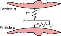
Figure 3: Spring–slider system at the contact between particles $p$ and $q$.

These local mechanical force increments, as well as the entire mechanical stiffness $[\mathbf{H}^{\text{m}}]$, depend, of course, on the contacts’ stiffnesses. The stiffness of a contact $pq$ is expressed with a force–displacement mapping that gives the objective increment of contact force $\mathfrak{d}\mathbf{f}^{pq}$ (and moment $\mathfrak{d}\mathbf{m}^{pq}$) as a function of the objective increments of the relative contact displacement $\delta\mathbf{u}^{\text{def},pq}$ (and the relative contact rotation $\delta\boldsymbol{\theta}^{\text{def},pq}$). The relative displacement and relative rotation will deform the two particles at their contact and are defined by the kinematic relations

$$\delta\mathbf{u}^{\text{def},pq} =d\mathbf{u}^{q}-d\mathbf{u}^{p}+\left(d\boldsymbol{\theta}^{q}\times\mathbf{r}^{pq,q}-d\boldsymbol{\theta}^{p}\times\mathbf{r}^{pq,p}\right)$$ (17)

$$\delta\boldsymbol{\theta}^{\text{def},pq} =d\boldsymbol{\theta}^{q}-d\boldsymbol{\theta}^{p}$$ (18)

where $\mathbf{r}^{pq,p}$ and $\mathbf{r}^{pq,q}$ are the contact vectors from the material points $\chi^{p}$ and $\chi^{q}$ to the contact point $c$ (note that $\delta\mathbf{u}^{\text{def},pq}=-\delta\mathbf{u}^{\text{def},qp}$ and $\delta\boldsymbol{\theta}^{\text{def},pq}=-\delta\boldsymbol{\theta}^{\text{def},qp}$). These relations between contact movements and particle movements can be gathered into the matrix form

$$\left[\begin{array}[]{@{\extracolsep{\fill}}c@{\extracolsep{\fill}}}\delta\mathbf{u}^{\text{def}}\\ \hdashline[1pt/1pt]\delta\boldsymbol{\theta}^{\text{def}}\end{array}\right]_{2(6M)\times 1}=\left[\mathbf{B}\right]_{2(6M)\times 6N}\left[\begin{array}[]{@{\extracolsep{\fill}}c@{\extracolsep{\fill}}}d\mathbf{u}\\ \hdashline[1pt/1pt]d\boldsymbol{\theta}\end{array}\right]_{6N\times 1}$$ (19)

where $[\mathbf{B}]$ is the kinematic matrix (or the rigidity matrix, as in [10, 11]), and the “$\delta$” vector on the left is of size $2(6)$ and contains both $pq$ and $qp$ variants. As a condition of equilibrium, $[\mathbf{A}]$ and $[\mathbf{B}]$ are dual, with $[\mathbf{A}]=[\mathbf{B}]^{\text{T}}$.

Both $\delta\mathbf{u}^{\text{def},pq}$ and $\delta\boldsymbol{\theta}^{\text{def},pq}$ are objective quantities and, as such, can be used in computing the objective force increments $\mathfrak{d}\mathbf{f}^{pq}$ and $\mathfrak{d}\mathbf{m}^{pq}$. We assume a surjective mapping from the full $\mathbb{R}^{6}$ space of a contact’s incremental deformation (in 3D, the 3-component $\delta\mathbf{u}^{\text{def},pq}$ and the 3-component $\delta\boldsymbol{\theta}^{\text{def},pq}$) into the possibly smaller space of incremental contact force and moment (the 3-component $\mathfrak{d}\mathbf{f}^{pq}$ and 3-component $\mathfrak{d}\mathbf{m}^{pq}$). This condition excludes Signorini and rigid-frictional models of contact behavior. We will assume, however, that the force–displacement relation is rate-independent, so that the mapping of displacement to force is homogeneous of degree one with respect to the relative contact displacement $\delta\mathbf{u}^{\text{def},pq}$ and rotation $\delta\boldsymbol{\theta}^{\text{def},pq}$, perhaps in the restricted functional form

$$\mathfrak{d}\mathbf{f}^{pq} =\mathbf{F}^{pq}\left(\frac{\delta\mathbf{u}^{\text{def},pq}}{|\delta\mathbf{u}^{\text{def},pq}|}\,,\,\mathbf{f}^{pq}\right)\cdot\delta\mathbf{u}^{\text{def},pq}$$ (20)

$$\mathfrak{d}\mathbf{m}^{pq} =\mathbf{M}^{pq}\left(\frac{\delta\boldsymbol{\theta}^{\text{def},pq}}{|\delta\boldsymbol{\theta}^{\text{def},pq}|}\,,\,\mathbf{m}^{pq}\right)\cdot\delta\boldsymbol{\theta}^{\text{def},pq}$$ (21)

noting that the stiffness matrices $\mathbf{F}^{pq}$ and $\mathbf{M}^{pq}$ might depend upon the direction of the relative displacement (and rotation) and on the current contact force (and moment). That is, in contrast with elasticity or with the smooth hypoelasticity of Truesdell [14, 15], the incremental force relation in Eq. (20) is non-smooth, as it depends on the movement $\delta\mathbf{u}^{\text{def},pq}$ and its direction $\delta\mathbf{u}^{\text{def},pq}/|\delta\mathbf{u}^{\text{def},pq}|$. The force–displacement can be irreversible, and an example two-branch frictional contact model is reviewed in Section 2.5 and is applied in the examples of Section 4. Other contact models, however, are even more general than Eqs. (20)–(21): for example, the force increment in a Cattaneo–Mindlin contact depends on the entire history of the force $\mathbf{f}^{pq}$ and not just on its current value [16].

Also embedded in Eqs. (20)–(21) is an assumption of locality in the contacts’ behaviors (e.g. [15], §26): the force of a contact $pq$ depends only on the movement $\delta\mathbf{u}^{\text{def},pq}$ of this contact and not on movements at other contacts within an assembly. This assumption allows the assembly of these relations into a block-diagonal matrix of contact stiffnesses,

$$\left[\begin{array}[]{@{\extracolsep{\fill}}c@{\extracolsep{\fill}}}\mathbf{F}^{pq}_{\;3\times 6}\\[0.43057pt] \hdashline[1pt/1pt]\mathbf{M}^{pq}_{\;3\times 6}\end{array}\right]_{6\times 6}\rightsquigarrow\left[\begin{array}[]{@{\extracolsep{\fill}}c@{\extracolsep{\fill}}}\mathbf{F}\\ \hdashline[1pt/1pt]\mathbf{M}\end{array}\right]_{2(6M)\times 2(6M)}$$ (22)

such that

$$\left[\begin{array}[]{@{\extracolsep{\fill}}c@{\extracolsep{\fill}}}\mathfrak{d}\mathbf{f}\\ \hdashline[1pt/1pt]\mathfrak{d}\mathbf{m}\end{array}\right]_{2(6M)\times 1}=\left[\begin{array}[]{@{\extracolsep{\fill}}c@{\extracolsep{\fill}}}\mathbf{F}\\ \hdashline[1pt/1pt]\mathbf{M}\end{array}\right]\left[\begin{array}[]{@{\extracolsep{\fill}}c@{\extracolsep{\fill}}}\delta\mathbf{u}^{\text{def}}\\ \hdashline[1pt/1pt]\delta\boldsymbol{\theta}^{\text{def}}\end{array}\right]=\left[\begin{array}[]{@{\extracolsep{\fill}}c@{\extracolsep{\fill}}}\mathbf{F}\\ \hdashline[1pt/1pt]\mathbf{M}\end{array}\right]\left[\mathbf{B}\right]\left[\begin{array}[]{@{\extracolsep{\fill}}c@{\extracolsep{\fill}}}d\mathbf{u}\\ \hdashline[1pt/1pt]d\boldsymbol{\theta}\end{array}\right]$$ (23)

noting again that the contents of $[\mathbf{F}/\mathbf{M}]$ may depend upon the current contact forces, $\mathbf{f}$ and $\mathbf{m}$, and on the directions of the incremental contact deformations, $\delta\mathbf{u}^{pq,\text{def}}$ and $\delta\boldsymbol{\theta}^{pq,\text{def}}$.

Combining Eqs. (7), (13), (14), and (23) yields the mechanical stiffness $[\mathbf{H}^{\text{m}}]$, which gives the contributions of the contact forces, $\mathfrak{d}\mathbf{f}$ and $\mathfrak{d}\mathbf{m}$, to the external forces, $d\mathbf{b}$ and $d\mathbf{w}$:

$$\left[\mathbf{H}^{\text{m}}\right]_{6N\times 6N}=\left[\mathbf{A}\right]_{6N\times 2(6M)}\left[\begin{array}[]{@{\extracolsep{\fill}}c@{\extracolsep{\fill}}}\mathbf{F}\\ \hdashline[1pt/1pt]\mathbf{M}\end{array}\right]_{2(6M)\times 2(6M)}\left[\mathbf{B}\right]_{2(6M)\times 6N}$$ (24)

in which the contact forces are collected with the statics matrix $[\mathbf{A}]$, as in Eq. (7).

The geometric “g-1” term in the equilibrium Eq. (16) arises from changes in the contact vector $\delta\mathbf{r}^{pq,p}$ when its contact point shifts across the particle $p$. This effect is illustrated in Fig. 4a, in which the flat surface of $p$ touches the round surface of $q$.

Figure 4: Geometric effects on internal forces: (a) alterations of $\mathbf{r}^{pq}$ and $\mathbf{r}^{qp}$ depend upon the curvatures of the particles at their contacts (see the discussion that precedes Eq. 25); (b) rolling of particle $q$ across $p$ alters the direction of the contact force (see the discussion that precedes Eq. 30); (c) rotations of $p$ and its contact force $\mathbf{f}^{pq}$ require an alteration of the external force, $d\mathbf{b}^{p}$ (see the discussion that precedes Eq. 34); and (d) a rotation of $p$ but an unrotated contact force $\mathbf{f}^{pq}$ requires an alteration of the external moment, $d\mathbf{w}^{p}$ (see the discussion that precedes Eq. 34).

The contact vector $\mathbf{r}^{pq,p}$ is lengthened when $q$ moves upward; whereas, vector $\mathbf{r}^{pq,q}$ is unchanged. These changes depend upon the curvatures of the two particles at their contact (e.g., with an opposite counterpart of Fig. 4a, in which $q$ is flat and $p$ is rounded, the $\mathbf{r}^{pq,q}$ would change with an upward movement of $q$, but $\mathbf{r}^{pq,p}$ would not, thus indicating the non-symmetry of this geometric effect). The increment $\delta\mathbf{r}^{pq,p}$ is a sum of normal and tangential parts:

$$\delta\mathbf{r}^{pq,p} =\delta\mathbf{r}^{\text{n},pq,p}+\delta\mathbf{r}^{\text{t},pq,p}$$ (25)

$$\delta\mathbf{r}^{\text{n},pq,p} =\frac{1}{2}\left(\delta\mathbf{u}^{\text{def},pq}\cdot\mathbf{n}^{pq}\right)\mathbf{n}^{pq}$$ (26)

$$\delta\mathbf{r}^{\text{t},pq,p} =-\left(\mathbf{K}^{pq,p}+\mathbf{K}^{pq,q}\right)^{\dagger}\cdot\left[\delta\boldsymbol{\theta}^{\text{def},pq}\times\mathbf{n}^{pq}-\mathbf{K}^{pq,q}\cdot\left(\delta\mathbf{u}^{\text{def},pq}-\left(\delta\mathbf{u}^{\text{def},pq}\cdot\mathbf{n}^{pq}\right)\mathbf{n}^{pq}\right)\right]$$ (27)

where $\mathbf{n}^{pq}$ is the contact normal vector directed outward from $p$ (Fig. 1), and $\mathbf{K}^{pq,p}$ and $\mathbf{K}^{pq,q}$ are the curvatures of the two particles’ surfaces at their shared contact point $pq$ (see [17, 2]). For the $pq$ and $qp$ variants of a contact, $\mathbf{n}^{pq}=-\mathbf{n}^{pq}$, $\mathbf{K}^{pq,p}=\mathbf{K}^{qp,p}$, and $\mathbf{K}^{qp,q}=\mathbf{K}^{qp,q}$. The curvature matrices are singular, as they are surjective mappings from the three-dimensional space of contact movements onto the two-dimensional contact tangent plane, and a generalized inverse, such as the Moore-Penrose “$\,\dagger\,$” inverse must be used in Eq. (27) [17]. The “g-1” terms in Eq. (16) only affect moment equilibrium and depend linearly on the movements $d\mathbf{u}^{p}$, $d\mathbf{u}^{q}$, $d\boldsymbol{\theta}^{p}$, and $d\boldsymbol{\theta}^{q}$. These terms can be gathered into a contact stiffness $[\mathbf{H}^{\text{g-1}}]$:

$$\left.\begin{array}[]{l}\mathbf{0}\\ -\delta\mathbf{r}^{pq,p}\times\mathbf{f}^{pq}\end{array}\right\}_{6\times 1}\rightsquigarrow\left[\mathbf{H}^{\text{g-1}}\right]_{6N\times 6N}\left[\begin{array}[]{@{\extracolsep{\fill}}c@{\extracolsep{\fill}}}d\mathbf{u}\\ \hdashline[1pt/1pt]d\boldsymbol{\theta}\end{array}\right]_{6N\times 1}$$ (28)

where the stiffness gives changes in the forces at the $M$ contacts produced by movements of the $N$ particles. The $3\times 1$ zero vector on the left represents the nil contribution of this geometric effect on the force equilibrium of $p$. The unsymmetric arrangement on the left of Eq. (28) leads to a non-symmetric stiffness $[\mathbf{H}^{\text{g-1}}]$.

Comparing Eqs. (9) and (28), we see that $[\mathbf{H}^{\text{g-1}}]$ expresses the effect of changes in the static matrix upon the incremental equilibrium:

$$\left[\mathbf{H}^{\text{g-1}}\right]\left[d\mathbf{x}\right]=\left[\rule{0.0pt}{9.47217pt}(\partial\mathbf{A}/\partial\mathbf{x})\cdot d\mathbf{x}\right]\left[\,\boldsymbol{\mathfrak{f}}\,\right]\quad\text{or}\quad H_{ij}^{\text{g-1}}dx_{j}=A_{ik,j}\mathfrak{f}_{k}dx_{j}$$ (29)

with $H_{ij}^{\text{g-1}}=A_{ik,j}\mathfrak{f}_{k}$.

The incremental change in the contact vector $\delta\mathbf{r}^{pq,p}$ in Eq. (25) is composed of two parts: a normal increment $\delta\mathbf{r}^{\text{n},pq,p}$ and a tangential increment $\delta\mathbf{r}^{\text{t},pq,p}$. Considering the two parts, the geometric stiffness $[\mathbf{H}^{\text{g-1}}]$ that originates from the normal increment will usually be insignificant, since the stiffness that is associated with this part is of order $|\boldsymbol{\mathfrak{f}}^{pq}|/(k\,|\mathbf{r}^{pq,p}|)$, where $k$ is the contact stiffness (Section 2.5) and $\boldsymbol{\mathfrak{f}}^{pq}$ is the contact force. This ratio is usually quite small for most materials (an exception might be gel-like particles with very soft contacts). However, the stiffness that originates from the tangential increment $\delta\mathbf{r}^{\text{t},pq,p}$ is significant whenever rolling movements are large.

The “g-2” terms in Eqs. (15) and (16) account for the changes, $\delta\hat{\mathbf{f}}^{pq}$ and $\delta\hat{\mathbf{m}}^{pq}$, in the contact forces that are produced by rotations of the contact normal $d\mathbf{n}^{pq}$. In Fig. 4b, particle $q$ rolls across $p$ while maintaining the magnitude of its contact force, although the rolling of $q$ rotates the force. Even though the relative contact movements $\delta\mathbf{u}^{\text{def},pq}$ and $\delta\boldsymbol{\theta}^{\text{def},pq}$ are zero during a rolling movement (thus producing no deformation forces $\mathfrak{d}\mathbf{f}^{pq}$ and $\mathfrak{d}\mathbf{m}^{pq}$), the contact force is altered by its rotation, and this change in the contact force must be counteracted by a change in the external force, $d\mathbf{b}^{p}$. The internal force $\mathbf{f}^{pq}$ is a circulatory, follower force, and one would expect the stiffness matrix $[\mathbf{H}]$ of this two-particle system to be non-symmetric. A similar condition is produced between two particles that twirl and waltz as a joined pair, since their contact force will rotate in unison with the pair’s motions. These force alterations are expressed as

$$\delta\hat{\mathbf{f}}^{pq} =\mathbf{f}^{pq}\times\left(\delta\mathbf{n}^{pq}\times\mathbf{n}^{pq}\right)-\frac{1}{2}\left(\delta\boldsymbol{\theta}^{\text{def},pq}\cdot\mathbf{n}^{pq}\right)\mathbf{f}^{pq}\times\mathbf{n}^{pq}$$ (30)

$$\delta\hat{\mathbf{m}}^{pq} =\mathbf{m}^{pq}\times\left(\delta\mathbf{n}^{pq}\times\mathbf{n}^{pq}\right)-\frac{1}{2}\left(\delta\boldsymbol{\theta}^{\text{def},pq}\cdot\mathbf{n}^{pq}\right)\mathbf{m}^{pq}\times\mathbf{n}^{pq}$$ (31)

where rolling produces a rotation of the contact normal $\delta\mathbf{n}^{pq}$ (as seen from the perspective of an observer attached to $p$) that depends upon the particles’ curvatures [17],

$$\delta\mathbf{n}^{pq}=-\mathbf{K}^{pq,p}\cdot\delta\mathbf{r}^{\text{t},pq,p}$$ (32)

where $\delta\mathbf{r}^{\text{t},pq,p}$ is defined in Eq. (27). After substituting Eqs. (30), (31), and (32), the “g-2” terms in Eqs. (15) and (16) depend linearly on the movements $d\mathbf{u}^{p}$, $d\mathbf{u}^{q}$, $d\boldsymbol{\theta}^{p}$, and $d\boldsymbol{\theta}^{q}$, and these terms can be gathered into a contact stiffness matrix $[\mathbf{E}^{\text{g-2}}]$ and an assembly stiffness matrix $[\mathbf{H}^{\text{g-2}}]$:

$$\left.\begin{aligned} &\,\delta\hat{\mathbf{f}}^{pq}\\ &\delta\hat{\mathbf{m}}^{pq}\end{aligned}\right\}_{6\times 1}\rightsquigarrow\left[\mathbf{E}^{\text{g-2}}\right]_{2(6M)\times 6N}\left[\begin{array}[]{@{\extracolsep{\fill}}c@{\extracolsep{\fill}}}d\mathbf{u}\\ \hdashline[1pt/1pt]d\boldsymbol{\theta}\end{array}\right]\quad\text{and}\quad\left[\mathbf{H}^{\text{g-2}}\right]_{6N\times 6N}=\left[\mathbf{A}\right]\left[\mathbf{E}^{\text{g-2}}\right]$$ (33)

where $[\mathbf{A}]$ is the statics matrix of Eq. (7). Stiffness $[\mathbf{H}^{\text{g-2}}]$ is clearly non-symmetric.

Equations (12₁) and (12₂) yield the co-rotated external force increments $\delta\mathbf{b}^{p}$ and $\delta\mathbf{w}^{p}$, as would be seen by an observer attached to $p$. The geometric “g-3” terms in Eqs. (15) and (16) recover the global increments $d\mathbf{b}^{p}$ and $d\mathbf{w}^{p}$ by applying Eq. (11) to the forces $\mathbf{b}^{p}$ and $\mathbf{w}^{p}$. Figure 4c shows a single particle $p$ with external force $\mathbf{b}^{p}$ and a counteracting contact follower force $\mathbf{f}^{pq}$ that rotates with the particle. If the contact is undeformed, the material increment $\mathfrak{d}\mathbf{f}^{pq}$ is zero, and if no rolling occurs at the contact, the directions of the contact normal and contact force will appear unchanged when viewed by an observer who rotates with the particle (i.e., $\delta\mathbf{n}^{pq}=\delta\mathbf{f}^{pq}=\mathbf{0}$). Yet, the force $\mathbf{f}^{pq}$ rotates within the global frame. This rotation is produced by the “g-3” term $d\boldsymbol{\theta}^{p}\times\mathbf{f}^{pq}$: that is, to maintain equilibrium after the small rotation $d\boldsymbol{\theta}^{p}$, the external force $\mathbf{b}^{p}$ must rotate to $\mathbf{b}^{p}+d\mathbf{b}^{p}$.

As another example, Fig. 4d shows a contact force $\mathbf{f}^{pq}$ that remains vertical: perhaps a perfect rolling has shifted the contact point while inducing no contact deformation, so that $\mathfrak{d}\mathbf{f}^{pq}=d\mathbf{f}^{pq}=\mathbf{0}$. However, an observer attached to the particle would see a rotation of the contact force, with $\delta\hat{\mathbf{f}}^{pq}\neq 0$. The $d\boldsymbol{\theta}^{p}\times\mathbf{f}^{pq}$ term in Eq. (15) nullifies this increment, so that $d\mathbf{f}^{pq}=d\mathbf{b}^{p}=0$. Yet, the $\mathbf{r}^{pq}\times\delta\hat{\mathbf{f}}^{pq}$ term in Eq. (16) yields the counteracting external moment $d\mathbf{w}^{p}$ that is required to maintain equilibrium.

The “g-3” terms in Eqs. (15) and (16) depend linearly on the movements $d\mathbf{u}^{p}$, $d\mathbf{u}^{q}$, $d\boldsymbol{\theta}^{p}$, and $d\boldsymbol{\theta}^{q}$, and these terms can be gathered into the assembly stiffness matrix $[\mathbf{H}^{\text{g-3}}]$:

$$\left.\begin{aligned} &-d\boldsymbol{\theta}^{p}\times\mathbf{f}^{pq}\\ &-d\boldsymbol{\theta}^{p}\times\mathbf{m}^{pq}\end{aligned}\right\}_{6\times 1}\rightsquigarrow\left[\mathbf{H}^{\text{g-3}}\right]_{6N\times 6N}\left[\begin{array}[]{@{\extracolsep{\fill}}c@{\extracolsep{\fill}}}d\mathbf{u}\\ \hdashline[1pt/1pt]d\boldsymbol{\theta}\end{array}\right]$$ (34)

The matrix $[\mathbf{H}^{\text{g-3}}]$ is non-symmetric.

We complete the derivation of stiffness $[\mathbf{H}]$ by considering a possible dependence of the external forces $[\mathbf{b}]$ and $[\mathbf{w}]$ on the particles’ positions $[\mathbf{u}]$ and $[\boldsymbol{\theta}]$, as in Eq. (3)–(5) and Fig. 2. The matrix $[\partial\mathbf{p}/\partial\mathbf{x}]$ in Eq. (4) applies to position-dependent forces and is the fourth geometric stiffness,

$$\left[\mathbf{H}^{\text{g-4}}\right]_{6N\times 6N}=-\left[\partial\mathbf{p}/\partial\mathbf{x}\right]_{6N\times 6N}$$ (35)

On the other hand, when all external loads are independent of the particles’ positions (as with non-follower dead loads), the problem is simplified, with $[\mathbf{H}^{\text{g-4}}]=[\mathbf{0}]$, $[\mathbf{Q}]=[\mathbf{I}]$, and $[d\boldsymbol{\mathfrak{p}}]=[d\mathbf{q}]=[d\mathbf{p}]$.

Combining Eqs. (9), (10), (13), (14), (23), (24), and (33)–(5), the stiffness matrix $[\mathbf{H}]$ in Eq. (10) is the sum of mechanical and geometric parts, the latter being the sum of four influences:

$$\left[\mathbf{H}(\boldsymbol{\nu})\right]\left[d\mathbf{x}\right]=\left[d\boldsymbol{\mathfrak{p}}\right]$$ (36)

$$\left[\mathbf{H}(\boldsymbol{\nu})\right]=\left[\mathbf{H}^{\text{m}}(\boldsymbol{\nu})\right]+\left[\mathbf{H}^{\text{g}}\right]$$ (37)

$$\left[\mathbf{H}^{\text{g}}\right]=\left[\mathbf{H}^{\text{g-1}}\right]+\left[\mathbf{H}^{\text{g-2}}\right]+\left[\mathbf{H}^{\text{g-3}}\right]+\left[\mathbf{H}^{\text{g-4}}\right]$$ (38)

In the first two equations, we allow for inelastic and incrementally nonlinear contact behavior, in which the mechanical stiffness $[\mathbf{H}^{\text{m}}(\boldsymbol{\nu})]$ depends on the direction of loading, as expressed with the direction cosines $[\boldsymbol{\nu}]=[d\mathbf{x}]/\sqrt{[d\mathbf{x}]^{\text{T}}[d\mathbf{x}]}$. This possibility is expressed in Eqs. (20)–(21), where the increment in contact force depends on the direction of the contact movement (this dependence is developed in Sections 2.5 and 2.6).

The total stiffness is altered by geometric changes of the assembly that accompany the particle movements. The use of separate mechanical and geometric stiffnesses is an established concept in finite element analysis [18, 19], and Maier [20] designated their separate tendencies for instability as “physical instabilizing effects” and “geometrical instabilizing effects.” The three stiffnesses “g-1”, “g-2”, and “g-3” have an internal origin, as they arise from the shifting and rotation of the current contact forces among particles. These three stiffnesses depend upon (and are proportional to) the current forces and the particles’ sizes and surface curvatures. Stiffness “g-4” accounts for any position-dependent rotations of external follower forces. All four geometric stiffness matrices can be non-symmetric, which, by itself, would lead to a non-symmetric total stiffness $[\mathbf{H}]$. When one or more contacts reach the friction limit (see Section 2.5), non-symmetry of the mechanical stiffness $[\mathbf{H}^{\text{m}}]$ also contributes to non-symmetry of the total stiffness.

2.3 Stability framework

We use the thermodynamic approach of Bažant [21, 6], Petryk [22], and Nicot et al. [12] to investigate the stability of granular systems, an approach that will place stability in the context of the stiffness matrix $[\mathbf{H}]$ defined in Eqs. (10) and (36). Unlike previous works, we apply these principles in the context of a granular system, by explicitly accounting for the internal geometric effects that are due to the shapes of particles at their contact points, as embodied in the $[\mathbf{H}^{\text{g}}]$ geometric stiffness. Our restrictive approach is a systematic application of the principle of stationary total potential energy, commonly used in structural analysis (e.g., [13]). The approach considers the kinetic energy $E$ of a system that is initially in equilibrium in the reference configuration $[\mathbf{x}^{\ast}]=[\mathbf{u}^{\ast}/\boldsymbol{\theta}^{\ast}]$ at time $t^{\ast}$ and with no initial rate, $d\mathbf{x}/dt=0$ at $t^{\ast}$. As such, the analysis leads to a criterion for initial, incipient instability but does not fully characterize the subsequent dynamics, such as the flutter instability of non-conservative systems.

Following the notation of Nicot et al. [12], at time $t\geq t^{\ast}$, the rate of change of kinetic energy (i.e., the first variation of the total potential energy) is the difference in the work rates of the external forces $\mathbf{p}$ and internal forces $\boldsymbol{\mathfrak{f}}$,

$$\dot{E}(t)=\dot{W}_{\text{ext}}(t)-\dot{W}_{\text{int}}(t) =\left[\mathbf{p}(t)\right]^{\text{T}}\left[\dot{\mathbf{x}}\right]-\left[\boldsymbol{\mathfrak{f}}(t)\right]^{\text{T}}_{2(6M)\times 1}\left[\dot{\mathbf{u}}^{\text{def}}\right]$$ (39)

$$=\left[\mathbf{p}(t)\right]^{\text{T}}\left[\dot{\mathbf{x}}\right]-\left[\boldsymbol{\mathfrak{f}}(t)\right]^{\text{T}}\left[\mathbf{B}\right]\left[\dot{\mathbf{x}}\right]$$ (40)

where the vector of contact movements $[\dot{\mathbf{u}}^{\text{def}}]$ is abbreviated to include the displacement and rotation rates, $\dot{\mathbf{u}}^{\text{def},pq}$ and $\dot{\boldsymbol{\theta}}^{\text{def},pq}$, of Eqs. (17) and (18). In Eq. (40), contact velocities $\dot{\mathbf{u}}^{\text{def}}$ have been replaced with particle velocities $\dot{\mathbf{x}}$, by applying Eq. (19). The work done by internal contact forces can include both elastic and frictional (reversible and irreversible) parts, and these forces need not be derived from an elastic energy (or state) function, provided that the forces $\mathbf{p}(t)$ and $\boldsymbol{\mathfrak{f}}(t)$ are consistent with the directions of the movements $\dot{\mathbf{x}}$ (see Section 2.6).

Although Eq. (39) takes $\dot{E}$ as a rate of change of kinetic energy (e.g. [12]), similar results are found by taking $\dot{E}$ as the rate of the internal or free energy of a isotropic or adiabatic system (as in [21]) or as the rate of total potential energy associated with a deformed body and its loading system (e.g. [22]).

We will follow a general approach and allow external follower forces, using Eq. (36) instead of Eq. (10). If the external forces are rate-independent, then their values at $t=t^{\ast}+\Delta t$ depend only on the particles’ positions and on the loading increments, and they can be approximated with the series

$$[\mathbf{p}(t^{\ast}+\Delta t)]_{6N\times 1} =[\mathbf{p}(t^{\ast})]+\left[\frac{\partial\mathbf{p}}{\partial\mathbf{x}}(t^{\ast})\right]\left[\Delta\mathbf{x}\right]_{6N\times 1}+\left[\frac{\partial\mathbf{p}}{\partial\mathbf{q}}(t^{\ast})\right]\left[\Delta\mathbf{q}\right]_{L\times 1}+\ldots$$ (41)

$$\left[\,\boldsymbol{\mathfrak{f}}(t^{\ast}+\Delta t)\right]_{2(6M)\times 1} =\left[\,\boldsymbol{\mathfrak{f}}(t^{\ast})\right]+\left[\frac{\partial\boldsymbol{\mathfrak{f}}}{\partial\mathbf{x}}(t^{\ast})\right]\left[\Delta\mathbf{x}\right]_{6N\times 1}+\ldots$$ (42)

$$[\mathbf{B}(t^{\ast}+\Delta t)]_{2(6M)\times 6N} =[\mathbf{B}(t^{\ast})]+\left[\frac{\partial\mathbf{B}}{\partial\mathbf{x}}(t^{\ast})\right]\left[\Delta\mathbf{x}\right]_{6N\times 1}+\ldots$$ (43)

which we truncate at the second-order terms.The particle displacements $[\Delta\mathbf{x}]=[\Delta\mathbf{u}/\Delta\boldsymbol{\theta}]$ occur during the interval $\Delta t$, and the forces at $t^{\ast}+\Delta t$ are assumed to satisfy equilibrium in the displaced configuration (note the absence of both mass and damping). The last term in Eq. (42) corresponds to the internal force increments $d\mathbf{f}^{pq}$ and $d\mathbf{m}^{pq}$ that appear in Eqs. (13) and (14), and these increments are produced by a combination of contact deformations (i.e., the mechanical changes $\mathfrak{d}\mathbf{f}^{pq}$ and $\mathfrak{d}\mathbf{m}^{pq}$), of force rotations that accompany the contact movements (the geometric changes $\delta\hat{\mathbf{f}}^{pq}$ and $\delta\hat{\mathbf{m}}^{pq}$), and of frame rotations, $d\boldsymbol{\theta}^{p}\times\mathbf{f}^{pq}$ and $d\boldsymbol{\theta}^{p}\times\mathbf{m}^{pq}$. Combining these parts from Eqs. (23), (33), and (34),

$$\left[\frac{\partial\boldsymbol{\mathfrak{f}}}{\partial\mathbf{x}}(t^{\ast})\right]\left[\Delta\mathbf{x}\right]=\left[\begin{array}[]{@{\extracolsep{\fill}}c@{\extracolsep{\fill}}}\mathbf{F}(t^{\ast})\\ \hdashline[1pt/1pt]\mathbf{M}(t^{\ast})\end{array}\right]\left[\mathbf{B}(t^{\ast})\right]\left[\Delta\mathbf{x}\right]+\left[\mathbf{E}^{\text{g-2}}(t^{\ast})\right]\left[\Delta\mathbf{x}\right]+\left[\mathbf{E}^{\text{g-3}}(t^{\ast})\right]\left[\Delta\mathbf{x}\right]$$ (44)

where $[\mathbf{E}^{\text{g-3}}]_{2(6M)\times 6N}$ is an intermediate matrix, such that $[\mathbf{H}^{\text{g-3}}]=[\mathbf{A}][\mathbf{E}^{\text{g-3}}]$. On the right side of Eq. (41), the second and third terms include the explicit loading changes and geometric alterations in Eq. (4), such that

$$\left[\frac{\partial\mathbf{p}}{\partial\mathbf{x}}(t^{\ast})\right]\left[\Delta\mathbf{x}\right]=-\left[\mathbf{H}^{\text{g-4}}(t^{\ast})\right]\left[\Delta\mathbf{x}\right]\quad\text{and}\quad\left[\frac{\partial\mathbf{p}}{\partial\mathbf{q}}(t^{\ast})\right]\left[\Delta\mathbf{q}\right]=\left[\mathbf{Q}(t^{\ast})\right]\left[\Delta\mathbf{q}\right]$$ (45)

Continuing with the notation of Nicot et al. [12], the second time-derivative of the kinetic energy in Eq. (39) is

$$\ddot{E}=\left[\mathbf{p}(t)\right]^{\text{T}}\left[\ddot{\mathbf{x}}\right]-\left[\boldsymbol{\mathfrak{f}}(t)\right]^{\text{T}}\left[\mathbf{B}\right]\left[\ddot{\mathbf{x}}\right]+\left[\frac{d}{dt}\mathbf{p}(t)\right]^{\text{T}}\left[\dot{\mathbf{x}}\right]-\left[\frac{d}{dt}\boldsymbol{\mathfrak{f}}(t)\right]^{\text{T}}\left[\mathbf{B}\right]\left[\dot{\mathbf{x}}\right]-\left[\boldsymbol{\mathfrak{f}}(t)\right]^{\text{T}}\left[\frac{d}{dt}\mathbf{B}\right]\left[\dot{\mathbf{x}}\right]$$ (46)

This second derivative can also be viewed as the second variation of the total potential energy for isentropic conditions or of the total Helmholtz energy for isothermal conditions [21]. Substituting Eqs. (41)–(45),

$$\ddot{E}= \left(\left[\mathbf{p}(t^{\ast})\right]^{\text{T}}-\left[\boldsymbol{\mathfrak{f}}(t^{\ast})\right]^{\text{T}}\left[\mathbf{B}\right]\right)\left[\ddot{\mathbf{x}}\right]$$ (47)

$$-\left[\Delta\mathbf{x}\right]^{\text{T}}\left[\mathbf{H}^{\text{g-4}}(t^{\ast})\right]^{\text{T}}\left[\ddot{\mathbf{x}}\right]-\frac{d}{dt}\left[\Delta\mathbf{x}\right]^{\text{T}}\left[\mathbf{H}^{\text{g-4}}(t^{\ast})\right]^{\text{T}}\left[\dot{\mathbf{x}}\right]$$

$$-\left[\Delta\mathbf{x}\right]^{\text{T}}\left(\left[\mathbf{B}(t^{\ast})\right]^{\text{T}}\left[\begin{array}[]{@{\extracolsep{\fill}}c@{\extracolsep{\fill}}}\mathbf{F}(t^{\ast})\\ \hdashline[1pt/1pt]\mathbf{M}(t^{\ast})\end{array}\right]^{\text{T}}+\left[\mathbf{E}^{\text{g-2}}(t^{\ast})\right]^{\text{T}}+\left[\mathbf{E}^{\text{g-3}}(t^{\ast})\right]^{\text{T}}\right)\left[\mathbf{B}\right]\left[\ddot{\mathbf{x}}\right]$$

$$-\frac{d}{dt}\left[\Delta\mathbf{x}\right]^{\text{T}}\left(\left[\mathbf{B}(t^{\ast})\right]^{\text{T}}\left[\begin{array}[]{@{\extracolsep{\fill}}c@{\extracolsep{\fill}}}\mathbf{F}(t^{\ast})\\ \hdashline[1pt/1pt]\mathbf{M}(t^{\ast})\end{array}\right]^{\text{T}}\!\!\!+\left[\mathbf{E}^{\text{g-2}}(t^{\ast})\right]^{\text{T}}\!\!\!+\left[\mathbf{E}^{\text{g-3}}(t^{\ast})\right]^{\text{T}}\right)\left[\mathbf{B}\right]\left[\dot{\mathbf{x}}\right]$$

$$+\left[\Delta\mathbf{q}\right]^{\text{T}}\left[\mathbf{Q}(t^{\ast})\right]^{\text{T}}\left[\ddot{\mathbf{x}}\right]+\frac{d}{dt}\left[\Delta\mathbf{q}\right]^{\text{T}}\left[\mathbf{Q}(t^{\ast})\right]^{\text{T}}\left[\dot{\mathbf{x}}\right]$$

$$-\left[\,\boldsymbol{\mathfrak{f}}(t^{\ast})\right]^{\text{T}}\left[\frac{\partial\mathbf{B}}{\partial\mathbf{x}}(t^{\ast})\cdot\frac{d}{dt}\Delta\mathbf{x}\right]\left[\dot{\mathbf{x}}\right]$$

The system is in equilibrium at time $t^{\ast}$, as in Eq. (7), which eliminates the right side of the first line in this equation. Because $[\mathbf{A}]=[\mathbf{B}]^{\text{T}}$, the various products $[\mathbf{E}]^{\text{T}}[\mathbf{B}]$ can be replaced with their $[\mathbf{H}]^{\text{T}}$ counterparts, as in Eq. (33₂). The last term in Eq. (47) is $B_{ij,k}f_{i}\frac{d}{dt}\Delta x_{k}\dot{x}_{j}$, but because $A_{ij}=B_{ji}$, the last term is equivalent to $A_{ij,k}f_{j}\frac{d}{dt}\Delta x_{k}\dot{x}_{i}=H^{\text{g-1}}_{ik}\frac{d}{dt}\Delta x_{k}\dot{x}_{i}$ (see Eq. 29), or

$$\left[\,\boldsymbol{\mathfrak{f}}(t^{\ast})\right]^{\text{T}}\left[\frac{\partial\mathbf{B}}{\partial\mathbf{x}}(t^{\ast})\cdot\frac{d}{dt}\Delta\mathbf{x}\right]\left[\dot{\mathbf{x}}\right]=\frac{d}{dt}\left[\Delta\mathbf{x}\right]^{\text{T}}\left[\mathbf{H}^{\text{g-1}}\right]^{\text{T}}\left[\dot{\mathbf{x}}\right]$$ (48)

Equation (47) applies at $t=t^{\ast}$, at which $[\Delta\mathbf{x}]=[\Delta\mathbf{q}]=[\mathbf{0}]$, which eliminates the $[\ddot{\mathbf{x}}]$ terms in Eq. (47), but we allow perturbations of the velocities and loading rates, with $(d/dt)[\Delta\mathbf{x}]=(1/\Delta t)[\Delta\mathbf{x}]=[\dot{\mathbf{x}}]\neq[\mathbf{0}]$ and $(d/dt)[\Delta\mathbf{q}]=(1/\Delta t)[\Delta\mathbf{q}]=[\dot{\mathbf{q}}]\neq[\mathbf{0}]$. As such, Eq. (47) is simplified as

$$\ddot{E}(t^{\ast})=\left[\dot{\mathbf{q}}\right]^{\text{T}}\left[\mathbf{Q}(t^{\ast})\right]^{\text{T}}\left[\dot{\mathbf{x}}\right]-\left[\dot{\mathbf{x}}\right]^{\text{T}}\left[\mathbf{H}(\boldsymbol{\nu},t^{\ast})\right]^{\text{T}}\left[\dot{\mathbf{x}}\right]$$ (49)

where the stiffness matrix $[\mathbf{H}(\boldsymbol{\nu})]$ is the sum of the mechanical stiffness $[\mathbf{H}^{\text{m}}(\boldsymbol{\nu})]$ and four non-conservative geometric contributions, as in Eqs. (37)–(38). Note that the possible dependence of stiffness $[\mathbf{H}]$ on loading direction $[\boldsymbol{\nu}]$ is included in this equation.

The kinetic energy at $t^{\ast}+\Delta t$ is estimated with the series

$$E(t^{\ast}+\Delta t)=E(t^{\ast})+\dot{E}(t^{\ast})+\frac{1}{2}(\Delta t)^{2}\ddot{E}(t^{\ast})+\ldots$$ (50)

and because the system is assumed in equilibrium at $t^{\ast}$, with $\dot{E}(t^{\ast})=0$, the change in kinetic energy during increment $\Delta t$, excluding terms of order $(\Delta t)^{3}$ and higher, is due to the velocity perturbation $[\dot{\mathbf{x}}]$ in Eq. (49):

$$E(t^{\ast}+\Delta t)-E(t^{\ast})=\frac{(\Delta t)^{2}}{2}\left(\rule{0.0pt}{8.61108pt}\mathcal{B}_{2}(\dot{\mathbf{x}})-\mathcal{W}_{2}(\dot{\mathbf{x}})\right)$$ (51)

where

$$\mathcal{B}_{2}(\dot{\mathbf{x}})=\left[\dot{\mathbf{q}}\right]^{\text{T}}\left[\mathbf{Q}(t^{\ast})\right]^{\text{T}}\left[\dot{\mathbf{x}}\right]=\left[\dot{\boldsymbol{\mathfrak{p}}}\right]^{\text{T}}\left[\dot{\mathbf{x}}\right]\quad\text{or}\quad\mathcal{B}_{2}(\dot{\mathbf{x}})=\left[\dot{\mathbf{p}}\right]^{\text{T}}\left[\dot{\mathbf{x}}\right]$$ (52)

$$\mathcal{W}_{2}(\dot{\mathbf{x}})=\left[\dot{\mathbf{x}}\right]^{\text{T}}\left[\mathbf{H}(\boldsymbol{\nu},t^{\ast})\right]\left[\dot{\mathbf{x}}\right]$$ (53)

Of the two alternative forms in Eq. (52), the more general Eq. (52₁) applies with or without external follower forces; whereas, the more restrictive Eq. (52₂) only applies with non-follower (dead) force increments. Bažant [21, 6] developed a similar expression by viewing the difference $\mathcal{B}_{2}-\mathcal{W}_{2}$ as the rate of internal entropy production, $\dot{S}_{\text{in}}$. He noted that the product of this rate and the (always positive) temperature, $T\dot{S}_{\text{in}}$, represents an influx of kinetic energy.

When the difference $\mathcal{B}_{2}-\mathcal{W}_{2}$ is positive for some $\dot{\mathbf{x}}$, the system can suffer a spontaneous infusion — a quadratic increase — of kinetic energy when the particle velocities are perturbed in the particular direction of $\dot{\mathbf{x}}$. A negative difference means that small perturbances are met with a suppression of kinetic energy, restoring the system to equilibrium. The second-order work $\mathcal{W}_{2}$ is an indicator of stability, as negative values allow a quadratic increase in kinetic energy in the absence of any change in external loading — when $[\dot{\mathbf{q}}]$ or $[\dot{\mathbf{p}}]$ are zero — and the system, which was assumed to be in equilibrium, enters a dynamical domain of behavior [23]. Note that in the absence of dead or follower forces, this increase in kinetic energy is bounded by the system’s stored internal energy and is suppressed by dissipative friction. Also note that $\mathcal{W}_{2}$ is not an objective quantity, as different values of $\mathcal{W}_{2}$ will be measured by observers that are moving (rotating) relative to each other (see the discussion of Type IV constraint). Finally, it is possible to show, with a full dynamic treatment, that flutter can appear before a negative second-order work appears [24]. The question of stability is explored further in Section 3.3.

Prior to the 1960’s, the principle of stationary total potential energy was usually applied to elastic systems, in which the internal energy is a path-independent state function of the current displacement (notable exceptions are the Shanley column [25] and the linear comparison methods of Hill [26]). The rate $\ddot{E}$ in Eq. (49), however, applies to rate-independent inelastic systems and depends upon the direction $[\boldsymbol{\nu}]$ of the particles’ movements, and for such systems, the susceptibility to instability depends upon the direction of the perturbance $[\dot{\mathbf{x}}]$. For granular systems, this path-dependence originates with inelastic contacts, which impart an influence of the direction of a contact’s movement $d\mathbf{u}^{pq,\text{def}}$ on the contact stiffness $\mathbf{F}^{pq}$ (Eqs. 20–21). Rate $\ddot{E}$ is based, therefore, on the notion of a tangentially equivalent linear system in which a single stiffness $[\mathbf{H}]$ applies only to a particular domain of perturbation directions $[\boldsymbol{\nu}]=[\dot{\mathbf{x}}]/\sqrt{[\dot{\mathbf{x}}]^{\text{T}}[\dot{\mathbf{x}}]}$ (see [6]). The problem is somewhat simpler for the two-branch, incrementally non-linear contact model of Sections 2.5, as we can determine the stability of an assembly by investigating a finite number of piece-wise constant assembly stiffnesses (Section 2.6).

2.4 Displacement constraints

Particle movements can be restricted in various ways, and we describe four types of constraints, presented in the order of their increasing complexity. With these types of constraints, varying degrees of restriction are placed upon the displacement increments $[d\mathbf{x}]=[d\mathbf{u}/d\boldsymbol{\theta}]$. This does not mean that we neglect load-control (indeed, our fourth type is fully load-controlled), since the applied loading increments $[d\mathfrak{p}]$ on the right of Eqs. (10) and (36) are always assigned, whether they are zero or otherwise. However, displacement constraints will typically require that certain reaction forces be superposed on the applied loads to achieve the prescribed displacements.

Rather than using the method of Lagrange multipliers, we approach constrained systems by applying various generalized inverses, and the reader is referred to [27] for a review. In the following, we shorten the notation by writing the direction-dependent $[\mathbf{H}(\boldsymbol{\nu})]$ as simply $[\mathbf{H}]$, deferring until Section 2.6 the implications of incremental non-linearity.

Type I constraint:

With this simplest type of constraint, a subset of $r$ displacements and rotations are assigned pre-determined values — a common situation in structural mechanics. In the usual manner, the full set $[d\mathbf{x}]=[d\mathbf{u}/d\boldsymbol{\theta}]$ is partitioned into the $r$ constrained “c” movements $[d\mathbf{x}^{\text{c}}]$ and the $6N-r$ unconstrained free “f” movements $[d\mathbf{x}^{\text{f}}]$. To prevent rigid rotations of 3D (2D) assemblies, at least six (three) movements should be constrained, and these $[d\mathbf{x}^{c}]$ should preclude rigid translations and rotations. Likewise, the external forces $[d\boldsymbol{\mathfrak{p}}]$ are partitioned into lists, $[d\boldsymbol{\mathfrak{p}}^{\text{c}}]$ and $[d\boldsymbol{\mathfrak{p}}^{\text{f}}]$, that correspond to the complementary constrained and free displacements. The forces $[d\boldsymbol{\mathfrak{p}}^{\text{c}}]$ represent the reaction forces of constraint. Equation (10) is rearranged in the standard partitioned form

$$\left[\begin{array}[]{@{\extracolsep{0ex}}c;{1pt/1pt}c@{\extracolsep{\fill}}}\mathbf{H}^{\text{cc}}&\mathbf{H}^{\text{cf}}\\ \hdashline[1pt/1pt]\mathbf{H}^{\text{fc}}&\mathbf{H}^{\text{f{}f}}\end{array}\right]\left[\begin{array}[]{l@{\extracolsep{\fill}}}d\mathbf{x}^{\text{c}}_{r\times 1}\\ \hdashline[1pt/1pt]d\mathbf{x}^{\text{f}}_{(6N-r)\times 1}\end{array}\right]=\left[\begin{array}[]{l@{\extracolsep{\fill}}}d\boldsymbol{\mathfrak{p}}^{\text{c}}_{r\times 1}\\ \hdashline[1pt/1pt]d\boldsymbol{\mathfrak{p}}^{\text{f}}_{(6N-r)\times 1}\end{array}\right]$$ (54)

and after shifting all response quantities to the left,

$$\left[\mathbf{U}\right]\left[\begin{array}[]{@{\extracolsep{\fill}}c@{\extracolsep{\fill}}}d\boldsymbol{\mathfrak{p}}^{\text{c}}\\ \hdashline[1pt/1pt]d\mathbf{x}^{\text{f}}\end{array}\right]=\left[\mathbf{V}\right]\left[\begin{array}[]{@{\extracolsep{\fill}}c@{\extracolsep{\fill}}}d\mathbf{x}^{\text{c}}\\ \hdashline[1pt/1pt]d\boldsymbol{\mathfrak{p}}^{\text{f}}\end{array}\right]$$ (55)

where

$$\left[\mathbf{U}\right]=\left[\begin{array}[]{@{\extracolsep{0ex}}c;{1pt/1pt}c@{\extracolsep{\fill}}}-\mathbf{I}&\mathbf{H}^{\text{cf}}\\ \hdashline[1pt/1pt]\mathbf{0}&\mathbf{H}^{\text{f{}f}}\end{array}\right]\quad\text{and}\quad\left[\mathbf{V}\right]=\left[\begin{array}[]{@{\extracolsep{0ex}}c;{1pt/1pt}c@{\extracolsep{\fill}}}-\mathbf{H}^{\text{cc}}&\mathbf{0}\\ \hdashline[1pt/1pt]-\mathbf{H}^{\text{fc}}&\mathbf{I}\end{array}\right]$$ (56)

which is solved with the usual method of static condensation. Note that separate $[\mathbf{Q}]$ matrices (Eq. 5) may be required for resolving the two sets of forces $[d\boldsymbol{\mathfrak{p}}^{\text{c}}]$ and $[d\boldsymbol{\mathfrak{p}}^{\text{f}\,}]$ when both sets are position-dependent (for example, platen displacements might be controlled while also controlling a membrane pressure).

Type II constraint:

As an intermediate case that will be used to derive the more general non-homogeneous Type III constraint, a set of $r$ linear holonomic homogeneous constraints is applied to the displacements and rotations $[d\mathbf{x}]$,

$$\left[\mathbf{C}\right]_{r\times 6N}\left[d\mathbf{x}\right]=\left[\mathbf{0}\right]_{r\times 1}$$ (57)

restricting $[d\mathbf{x}]$ to the null-space $\mathcal{L}$ of $[\mathbf{C}]$, such that $[d\mathbf{x}]\in\mathcal{L}=\mathcal{N}(\mathbf{[C]})$. We will assume that matrix $[\mathbf{C}]$ has full rank $r$. In 3D (2D), at least six (three) constraints are required, and these constraints should preclude rigid motions of the assembly. The matrices $[\mathbf{P}_{\mathcal{L}}]$ and $[\mathbf{P}_{\mathcal{L}^{\perp}}]$ project vectors $[d\mathbf{x}]$ onto the subspace $\mathcal{L}$ and its orthogonal complement:

$$\left[\mathbf{P}_{\mathcal{L}}\right] =\left[\,\mathbf{I}\,\right]_{6N}-[\mathbf{P}_{\mathcal{L}^{\perp}}]$$ (58)

$$[\mathbf{P}_{\mathcal{L}^{\perp}}] =\left[\,\mathbf{C}\,\right]^{\text{T}}\left(\left[\,\mathbf{C}\,\right]\left[\,\mathbf{C}\,\right]^{\text{T}}\right)^{-1}\left[\,\mathbf{C}\,\right]$$ (59)

where $[\mathbf{I}]_{6N}$ is the $6N\times 6N$ identity matrix. That is, $[\mathbf{P}_{\mathcal{L}}][d\mathbf{x}]$ projects vector $[d\mathbf{x}]$ onto the null-space of $[\mathbf{C}]$; whereas, $[\mathbf{P}_{\mathcal{L}^{\perp}}][d\mathbf{x}]$ projects $[d\mathbf{x}]$ onto the row-space of $[\mathbf{C}]$. Because $[\mathbf{C}]$ is assumed to have full rank, the inverse in Eq. (59) exists.

Considered together, Eqs. (36) and (57) can be cast in the alternative form

$$\left[\mathbf{H}\right]\left[d\mathbf{x}\right]-\left[d\mathbf{y}\right]=\left[d\boldsymbol{\mathfrak{p}}\right], \left[\mathbf{H}\right]\in\mathbb{R}^{6N\times 6N},\;\left[d\boldsymbol{\mathfrak{p}}\right]\in\mathbb{R}^{6N},$$ (60)

$$\left[d\mathbf{x}\right]\in\mathcal{L}=\mathcal{N}(\left[\mathbf{C}\right]),\;\left[d\mathbf{y}\right]\in\mathcal{L}^{\perp}$$

noting that $[d\boldsymbol{\mathfrak{p}}]$ can lie outside the range of $[\mathbf{H}]$, which requires amendment with the additional vector $[d\mathbf{y}]$, as explained below. The consistency (i.e. the existence of a solution) of this system is equivalent to the consistency of the equation

$$\left(\rule{0.0pt}{9.47217pt}\left[\mathbf{H}\right]\left[\mathbf{P}_{\mathcal{L}}\right]+\left[\mathbf{P}_{\mathcal{L}^{\perp}}\right]\right)\left[d\mathbf{z}\right]=\left[d\boldsymbol{\mathfrak{p}}\right]$$ (61)

as shown in [27, 28]. If matrix $([\mathbf{H}][\mathbf{P}_{\mathcal{L}}]+[\mathbf{P}_{\mathcal{L}^{\perp}}])$ is non-singular, then Eq. (60) is consistent for all external force increments $[d\boldsymbol{\mathfrak{p}}]$ and has the unique solution

$$\left[d\mathbf{x}\right]=\left[\mathbf{P}_{\mathcal{L}}\right]\left[d\mathbf{z}\right]=\left[\mathbf{H}\right]_{(\mathcal{L})}^{(-1)}\left[d\boldsymbol{\mathfrak{p}}\right],\quad\left[d\mathbf{y}\right]=-\left[d\boldsymbol{\mathfrak{p}}\right]+\left[\mathbf{H}\right]\left[d\mathbf{x}\right]$$ (62)

where $[\mathbf{H}]_{(\mathcal{L})}^{(-1)}$ is the Bott-Duffin constrained inverse of $[\mathbf{H}]$ on $\mathcal{L}$:

$$\left[\mathbf{H}\right]_{(\mathcal{L})}^{(-1)}=\left[\mathbf{P}_{\mathcal{L}}\right]\left(\rule{0.0pt}{9.47217pt}\left[\mathbf{H}\right]\left[\mathbf{P}_{\mathcal{L}}\right]+\left[\mathbf{P}_{\mathcal{L}^{\perp}}\right]\right)^{-1}$$ (63)

in which the prefactor $[\mathbf{P}_{\mathcal{L}}]$ projects the solution $[d\mathbf{z}]$ onto the admissible domain $\mathcal{L}$, so that $[d\mathbf{x}]$ satisfies Eq. (57).

The displacements $[d\mathbf{x}]$ in Eq. (62) comply with the displacement constraints of Eq. (57), and the force increments $[d\mathbf{y}]$ are the reaction forces of constraint (superposed on $[d\boldsymbol{\mathfrak{p}}]$) that are necessary to satisfy the constraints. Note that $[d\mathbf{x}]$ and $[d\mathbf{y}]$ belong to orthogonal spaces, as $[d\mathbf{x}]^{\text{T}}[d\mathbf{y}]=-[d\mathbf{z}]^{\text{T}}[\mathbf{P}_{\mathcal{L}}]^{\text{T}}(([\mathbf{H}][\mathbf{P}_{\mathcal{L}}]+[\mathbf{P}_{\mathcal{L}^{\perp}}])[d\mathbf{z}]-[\mathbf{H}][\mathbf{P}_{\mathcal{L}}][d\mathbf{z}])=[d\mathbf{z}]^{\text{T}}[\mathbf{P}_{\mathcal{L}}]^{\text{T}}[\mathbf{P}_{\mathcal{L}^{\perp}}][d\mathbf{z}]=0$, a result that is consistent with d’Alembert’s principle of virtual work.

Type III constraint:

A set of $r$ linear holonomic non-homogeneous constraints is applied to the displacements and rotations $[d\mathbf{x}]$,

$$\left[\mathbf{C}\right]_{r\times 6N}\left[d\mathbf{x}\right]=\left[d\mathbf{c}\right]_{r\times 1}$$ (64)

Types I and II are special cases of this constraint. Similar to Type II constraint, we seek a solution of the equations

$$\left[\mathbf{H}\right]\left[d\mathbf{x}\right]-\left[d\mathbf{y}\right] =\left[d\boldsymbol{\mathfrak{p}}\right]$$ (65)

$$\left[\mathbf{C}\right]\left[d\mathbf{x}\right] =\left[d\mathbf{c}\right]$$

We assume that the constraint matrix $[\mathbf{C}]$ is full rank and adequate to preclude rigid movements of the assembly. We also assume that the constraints are consistent, with $[d\mathbf{c}]$ in the range of $[\mathbf{C}]$, $[d\mathbf{c}]\in\mathcal{R}([\mathbf{C}])$. If Eq. (65₂) is consistent, then for any generalized $\{1\}$-inverse $[\mathbf{C}]^{(1)}$, $[\mathbf{C}][\mathbf{C}]^{(1)}[d\mathbf{c}]=[d\mathbf{c}]$, since a $\{1\}$-inverse satisfies the weak property $[\mathbf{C}][\mathbf{C}]^{(1)}[\mathbf{C}]=[\mathbf{C}]$. A consistent Eq. (65₂) has the general solution

$$\left[d\mathbf{x}\right]=\left[\mathbf{C}\right]^{(1)}\left[d\mathbf{c}\right]+\left(\left[\,\mathbf{I}\,\right]-\left[\mathbf{C}\right]^{(1)}\left[\mathbf{C}\right]\right)[d\mathbf{v}],\quad\forall[d\mathbf{v}]\in\mathbb{R}^{6N}$$ (66)

for arbitrary $[d\mathbf{v}]$ (see §2.1, [27]). That is, $[d\mathbf{x}]$ is the sum of a solution of the inhomogeneous Eq. (65₂) and any solution of its homogeneous complement, $[\mathbf{C}][d\mathbf{x}]=[\mathbf{0}]$. Substituting into Eq. (65₁),

$$\left[\mathbf{H}\right]\left(\left[\,\mathbf{I}\,\right]-\left[\mathbf{C}\right]^{(1)}\left[\mathbf{C}\right]\right)[d\mathbf{v}]-\left[d\mathbf{y}\right]=\left[d\boldsymbol{\mathfrak{p}}\right]-\left[\mathbf{H}\right]\left[\mathbf{C}\right]^{(1)}\left[d\mathbf{c}\right]$$ (67)

The matrix $([\mathbf{I}]-[\mathbf{C}]^{(1)}[\mathbf{C}])$ is idempotent and projects an arbitrary vector $[d\mathbf{v}]\in\mathbb{R}^{6N}$ onto the null space of $[\mathbf{C}]$. This projection might be non-orthogonal (skew), but if we choose the Moore–Penrose inverse $[\mathbf{C}]^{\dagger}=[\mathbf{C}]^{\text{T}}([\mathbf{C}][\mathbf{C}]^{\text{T}})^{-1}$ as the $\{1\}$-inverse, then the projection is orthogonal, and the projection matrices $[\mathbf{P}_{\mathcal{L}}]$ and $[\mathbf{P}_{\mathcal{L}^{\perp}}]$ in Eqs. (58) and (59) are used in place of $([\mathbf{I}]-[\mathbf{C}]^{(1)}[\mathbf{C}])$ and its complement. As such, Eq. (67) is equivalent to the system

$$\left(\rule{0.0pt}{9.47217pt}\left[\mathbf{H}\right]\left[\mathbf{P}_{\mathcal{L}}\right]+\left[\mathbf{P}_{\mathcal{L}^{\perp}}\right]\right)\left[d\mathbf{z}\right]=\left[d\boldsymbol{\mathfrak{p}}\right]-\left[\mathbf{H}\right]\left[\mathbf{C}\right]^{\dagger}\left[d\mathbf{c}\right]$$ (68)

If the sum $([\mathbf{H}][\mathbf{P}_{\mathcal{L}}]+[\mathbf{P}_{\mathcal{L}^{\perp}}])$ is non-singular, then

$$\begin{aligned} \left[d\mathbf{x}\right]&=\left[\mathbf{C}\right]^{\dagger}\left[d\mathbf{c}\right]+\left[\mathbf{P}_{\mathcal{L}}\right]\left[d\mathbf{z}\right]\\ &=\left[\mathbf{C}\right]^{\dagger}\left[d\mathbf{c}\right]+\left[\mathbf{P}_{\mathcal{L}}\right]\left(\rule{0.0pt}{8.61108pt}\left[\mathbf{H}\right]\left[\mathbf{P}_{\mathcal{L}}\right]+\left[\mathbf{P}_{\mathcal{L}^{\perp}}\right]\right)^{-1}\left(\left[d\boldsymbol{\mathfrak{p}}\right]-\left[\mathbf{H}\right]\left[\mathbf{C}\right]^{\dagger}\left[d\mathbf{c}\right]\right)\end{aligned}$$ (69)

$$\left[d\mathbf{y}\right]=-\left[d\boldsymbol{\mathfrak{p}}\right]+\left[\mathbf{H}\right]\left[d\mathbf{x}\right]$$ (70)

where $[d\mathbf{x}]$ is the solution vector of incremental displacements and rotations, and $[d\mathbf{y}]$ contains the incremental reaction forces of constraint (superposed on $[d\boldsymbol{\mathfrak{p}}]$) that are necessary to satisfy the movement constraints.

Type IV constraint:

We now consider the special case of no displacement constraints on the particles’ movements, which we call an isolated system. Isolated systems are the discrete analog of full load-control and were the sole focus of [2]. Type IV constraint (or lack of constraint) can be used to examine the intrinsic material behavior of an assembly, without the disrupting influence of platens or other displacement constraints.

Because such isolated systems are not anchored to a Gallilean foundation (imagine a granular asteroid tumbling through space), the stiffness matrix $[\mathbf{H}]$ is singular of rank $6N-6$, and Eq. (10) represents a bijective mapping from the quotient space of deformation-producing movements $[d\mathbf{x}]$ to the subspace of $[d\mathbf{p}]$ that is comprised only of equilibrium forces.

With the absence of any displacement constraints that would otherwise prevent rigid-body motions, two discrepancies arise when applying the stiffness relationship in Eqs. (10) and (36) and when applying the second-order work product $[d\mathbf{b}/d\mathbf{w}]^{\text{T}}[d\mathbf{u}/d\boldsymbol{\theta}]$ in Eq. (53). First, the use of the stiffness $[\mathbf{H}]$ in Eq. (10) will yield incorrect external forces $[d\mathbf{p}]=[d\mathbf{b}/d\mathbf{w}]$ when the displacements $[d\mathbf{x}]=[d\mathbf{u}/d\boldsymbol{\theta}]$ correspond to a rigid rotation of an entire isolated assembly, as the existing forces $[\mathbf{b}/\mathbf{w}]$ will rotate, in the manner of follower forces, during a rotation of the isolated assembly. Secondly, a rigid rotation of an isolated assembly (or alternatively, an observer rotation) will produce apparent alterations $[d\mathbf{p}]$ and $[d\mathbf{x}]$ that have a non-zero inner product, $[d\mathbf{p}]^{\text{T}}[d\mathbf{x}]\neq 0$. That is, the second-order work $\mathcal{W}_{2}$ in Eq. (53) is not objective.

A solution to the second discrepancy was proposed in [2], which involved projecting forces and movements onto a special subspace. Here, we resolve both discrepancies by using a generalized matrix inverse. Consider a $6N\times 6$ matrix $[\mathbf{R}]$ that shifts and rotates the entire assembly as a rigid body:

$$\left[\begin{array}[]{@{\extracolsep{\fill}}c@{\extracolsep{\fill}}}d\mathbf{u}^{\text{rigid}}\\ \hdashline[1pt/1pt]d\boldsymbol{\theta}^{\text{rigid}}\end{array}\right]_{6N\times 1}=\left[\mathbf{R}\right]_{6N\times 6}\left[\begin{array}[]{@{\extracolsep{\fill}}c@{\extracolsep{\fill}}}d\overline{\mathbf{u}}\\ \hdashline[1pt/1pt]d\overline{\boldsymbol{\theta}}\end{array}\right]_{6\times 1}$$ (71)

where $d\overline{\mathbf{u}}$ and $d\overline{\boldsymbol{\theta}}$ are the shift and rotation vectors that are applied uniformly to the entire assembly, and $d\mathbf{u}^{\text{rigid}}$ and $d\boldsymbol{\theta}^{\text{rigid}}$ are the resulting individual particle motions and rotations.

For an isolated system, we seek solutions of the stiffness Eq. (10) that preclude rigid-body motions, such that $[d\mathbf{x}]=[d\mathbf{u}/d\boldsymbol{\theta}]$ belongs to the left null-space of $[\mathbf{R}]$:

$$\left[\mathbf{R}\right]_{6\times 6N}^{\text{T}}\left[d\mathbf{x}\right]=\left[\mathbf{0}\right]_{6\times 1}$$ (72)

This restriction reduces the analysis of an isolated system to that of a system with homogeneous Type II constraints, as in Eq. (57), and we can follow a similar approach for finding solutions and for identifying stiffness pathologies. As with Eqs. (58)–(59), the matrices $[\mathbf{P}^{\text{r-r}}]$ and $[\mathbf{P}^{\text{n-r-r}}]$ project a general set of particle motions onto the sub-space of rigid-body motions and the sub-space that precludes rigid-body motions:

$$\left[\mathbf{P}^{\,\text{r-r}}\right]_{6N\times 6N} =\left[\mathbf{R}\right]\left(\left[\mathbf{R}\right]^{\text{T}}\left[\mathbf{R}\right]\right)^{-1}\left[\mathbf{R}\right]^{\text{T}}$$ (73)

$$\left[\mathbf{P}^{\,\text{n-r-r}}\right]_{6N\times 6N} =\left[\,\mathbf{I}\,\right]_{6N\times 6N}-\left[\mathbf{P}^{\text{r-r}}\right]$$ (74)

The consistency of the stiffness problem in Eqs. (10) and (36) along with the constraints of Eq. (72) is equivalent to consistency of the equation

$$\left(\rule{0.0pt}{9.47217pt}\left[\mathbf{H}\right]\left[\mathbf{P}^{\text{n-r-r}}\right]+\left[\mathbf{P}^{\text{r-r}}\right]\right)\left[d\mathbf{z}\right]=\left[d\boldsymbol{\mathfrak{p}}\right]$$ (75)

If the summed matrix on the left is non-singular, then this equation has the unique solution

$$[d\mathbf{x}] =\left[\mathbf{P}^{\text{n-r-r}}\right]\left(\rule{0.0pt}{9.47217pt}\left[\mathbf{H}\right]\left[\mathbf{P}^{\text{n-r-r}}\right]+\left[\mathbf{P}^{\text{r-r}}\right]\right)^{-1}\left[d\boldsymbol{\mathfrak{p}}\right]$$ (76)

$$[d\mathbf{y}] =-\left[d\boldsymbol{\mathfrak{p}}\right]+\left[\mathbf{H}\right][d\mathbf{x}]$$ (77)

where $[d\mathbf{y}]$ are the reaction forces of constraint, distributed among all particles in the system, that are required to prevent a rigid-body motion of the system. The matrix $([\mathbf{H}][\mathbf{P}^{\text{n-r-r}}]+[\mathbf{P}^{\text{r-r}}])$ in Eq. (75) can be used for examining questions of non-uniqueness and instability of granular systems (Section 3).

2.5 Linear-frictional contact model

Many constitutive models have been proposed for the contact force–displacement relationship between two bodies in contact, such as the general form of Eqs. (20)–(21). These models include the complex, history-dependent models of Cattaneo [29] and Mindlin [16] and of Kalker [30]; models that include resistive moments [31]; and models that include incipient, grazing contact. Among the simplest models is a zero-tension zero-moment contact with linear stiffnesses in both normal and tangential directions but with a frictional limit on the tangential force (for example, [32, 33]). This linear-frictional contact model with no contact moment is illustrated in Fig. 3 and is widely used in DEM simulations (e.g., [34]), and it and will be exclusively applied in the paper’s examples. With this model, the stiffness of a contact $pq$ is incrementally nonlinear with two branches: an elastic (no-slip) branch that is characterized with positive normal and tangential stiffnesses $k^{pq}$ and $\alpha k^{pq}$, and a sliding (slip) branch that is characterized by the friction coefficient $\mu^{pq}$. Whenever the friction limit is reached, the active branch is determined by the direction of the contact deformation $\delta\mathbf{u}^{pq,\text{def}}$. Sliding occurs when two conditions are met:

1. When the current contact force has reached the friction limit, satisfying the yield condition $G^{pq}=0$:

   $$G^{pq}=G(\mathbf{f}^{pq})=\left|\mathbf{f}^{pq}-(\mathbf{n}^{pq}\cdot\mathbf{f}^{pq})\mathbf{n}^{pq}\right|+\mu\mathbf{f}^{pq}\cdot\mathbf{n}^{pq}=0$$ (78)

   This yield condition depends upon the current contact force $\mathbf{f}^{pq}$, which must be known before the contact stiffness can be constructed. Sliding also requires the second condition.

2. When the contact deformation $\delta\mathbf{u}^{pq,\text{def}}$ is directed outward from the yield surface (in displacement space):

   $$S^{pq}=S(\mathbf{f}^{pq},\delta\mathbf{u}^{pq,\text{def}})=\mathbf{g}^{pq}\cdot\delta\mathbf{u}^{pq,\text{def}}>0$$ (79)

   where vector $\mathbf{g}^{pq}$ is normal to the yield surface:

   $$\mathbf{g}^{pq}=k\left(\alpha\mathbf{h}^{pq}+\mu\mathbf{n}^{pq}\right)$$ (80)

   and the unit sliding direction $\mathbf{h}^{pq}$ is tangent to the contact plane and aligned with the tangential component of the current force $\mathbf{f}^{pq}$:

   $$\mathbf{h}^{pq}=\frac{\mathbf{f}^{pq}-(\mathbf{n}^{pq}\cdot\mathbf{f}^{pq})\mathbf{n}^{pq}}{|\mathbf{f}^{pq}-(\mathbf{n}^{pq}\cdot\mathbf{f}^{pq})\mathbf{n}^{pq}|}$$ (81)

With this simple linear-frictional model and its hardening modulus of zero, the contact stiffness tensor $\mathbf{F}^{pq}$ in Eq. (20) has two branches, elastic and sliding (no-slip and slip), given by

$$\mathbf{F}^{pq}=\begin{cases}\mathbf{F}^{pq\text{, elastic}}=k\left[\alpha\mathbf{I}_{3}+(1-\alpha)\mathbf{n}^{pq}\otimes\mathbf{n}^{pq}\right]&\text{if }G^{pq}<0\text{ or }S^{pq}\leq 0\\ \mathbf{F}^{pq\text{, sliding}}=\mathbf{F}^{pq\text{, elastic}}-\mathbf{h}^{pq}\otimes\mathbf{g}^{pq}&\text{if }G^{pq}=0\text{ and }S^{pq}>0\end{cases}$$ (82)

where $\mathbf{I}_{3}$ is the $3\times 3$ identity matrix. Because the sliding and yield directions do not coincide ($\mathbf{h}^{pq}\neq\mathbf{g}^{pq}$), sliding is non-associative. The presence of the dyad $\mathbf{h}^{pq}\otimes\mathbf{g}^{pq}$ creates a non-symmetric contact stiffness in Eq. (82₂), leading to a non-symmetric global mechanical stiffness $[\mathbf{H}^{\text{m}}]$ whenever one or more contacts have reached the friction limit (with $G=0$) and are sliding (with $S>0$). The sliding behavior possesses deviatoric associativity, however, since the sliding direction $\mathbf{h}^{pq}$ is aligned with the tangential component of the yield surface normal $\mathbf{g}^{pq}$ [35].

Another characteristic embedded in Eq. (82) is the possibility of negative second-order work at a contact (i.e., contact weakening), in which the second-order quantity $\mathfrak{d}\mathbf{f}^{pq}\cdot\delta\mathbf{u}^{pq,\text{def}}$ becomes negative. Substituting Eqs. (80)–(81) and assuming $k>0$, the second-order work is negative at sliding contacts, $G^{pq}=0$, that meet the following displacement condition:

$$\delta\mathbf{u}^{\text{def}}\cdot\left[\mathbf{n}\otimes\mathbf{n}+\alpha\left(\mathbf{I}_{3}-\mathbf{n}\otimes\mathbf{n}-\mathbf{h}\otimes\mathbf{h}\right)-\mu\,\mathbf{h}\otimes\mathbf{n}\right]\cdot\delta\mathbf{u}^{\text{def}}<0\;\iff\;\mathfrak{d}\mathbf{f}^{pq}\cdot\delta\mathbf{u}^{pq,\text{def}}<0$$ (83)

an expression that we have shortened by removing the $pq$ superscripts. This condition, when expressed in sufficient abundance among the sliding contacts, can lead to a cumulative negative second-order work of the entire assembly (as in [3]). Equation (83) can be simplified by noting that $\delta\mathbf{u}\cdot(\mathbf{n}\otimes\mathbf{n})\cdot\delta\mathbf{u}$ equals the squared magnitude of the normal movement, $|\delta\mathbf{u}^{\text{n,def},pq}|^{2}$, and that the middle term is the squared magnitude of the component of movement that is orthogonal to both the contact normal and the current tangential force (i.e., the squared magnitude of the tangential component of movement that is orthogonal to the current tangential force, see Eq. 81):

$$\left|\delta\mathbf{u}^{\text{n,def},pq}\right|^{2}+\alpha\left|\delta\mathbf{u}^{\text{h}_{\perp},\text{def},pq}\right|^{2}-\mu\,\delta\mathbf{u}^{\text{def},pq}\cdot\left(\mathbf{h}^{pq}\otimes\mathbf{n}^{pq}\right)\cdot\delta\mathbf{u}^{\text{def},pq}>0\;\iff\;\mathfrak{d}\mathbf{f}^{pq}\cdot\delta\mathbf{u}^{pq,\text{def}}<0$$ (84)

Figure 5 summarizes the conditions for yielding (i.e., $G^{pq}=0$), for sliding ($S^{pq}>0$), and for negative second-order work, within a two-dimensional setting.

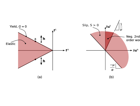
Figure 5: Conditions for yield, sliding, and negative second-order work in a two-dimensional setting: (a) admissible force domain and the friction limit for normal and tangential contact forces, $f^{\,\text{n},pq}$ and $f^{\,\text{t},pq}$. (b) for the case “a” of forward sliding, the conditions for sliding and for negative second-order work with respect to the normal and tangential contact movements, $\delta u^{\text{n},pq}$ and $\delta u^{\text{t},pq}$.

Negative second-order work can only occur when the contact is being unloaded in the normal direction ($\mathbf{n}^{pq}\cdot\delta\mathbf{u}^{\text{def},pq}>0$) while sliding continues in the direction of the current tangential force ($\mathbf{h}^{pq}\cdot\delta\mathbf{u}^{\text{def},pq}>0$).

We had earlier assumed that the mapping between the contact movement $\delta\mathbf{u}^{\text{def},pq}$ and the contact force increment $\mathfrak{d}\mathbf{f}^{pq}$ is homogeneous of degree 1 (see Eq. 20), and the stiffness in Eq. (82) is consistent with this assumption. Although the mapping is incrementally non-linear and is not additive, it is continuous, as the two stiffness branches produce the same increment increment $\mathfrak{d}\mathbf{f}^{pq}$ at the transition hyper-plane $S^{pq}=0$ [36].

2.6 Multiple stiffness branches

The geometric stiffness $[\mathbf{H}^{\text{g}}]$ in Eq. (37) is independent of the loading direction. However, the incremental mechanical stiffness $[\mathbf{H}^{\text{m}}]$ can depend upon the directions of movements at the contacts. For example, with the simple linear–frictional contact model, described in the previous section, both elastic and sliding contact stiffnesses are available at each contact that has reached the friction limit, so that the mechanical stiffness of the entire assembly, $[\mathbf{H}^{\text{m}}(\boldsymbol{\nu})]$, is incrementally nonlinear with multiple stiffness branches, whenever at least one contact has reached the friction limit. As a second example, certain models of contact rolling-friction involve four branches of stiffness for a single contact, due to the coupling of translational and rotational movements [37]. As another example, two particles can be in nascent contact with zero force, such that the particles’ incremental approach mobilizes the contact’s stiffness, but incremental withdrawal maintains the zero force. Such nascent (grazing) contacts have three stiffness branches: a non-slip approach, an approach that initiates slip, and a zero-stiffness withdrawal. In the following, we consider only the two-branch linear-frictional model of Section 2.5.

With linear-frictional contacts, the sliding conditions of all $M$ contacts can be collected in a single vector $[\boldsymbol{\mathfrak{s}}]$ by first gathering the vectors $\mathbf{g}^{pq}$ of Eq. (80) as the rows of a matrix $[\mathbf{G}]$,

$$\mathbf{g}^{pq}\rightsquigarrow\left[\mathbf{G}\right]_{2M\times 2(6M)}$$ (85)

but placing rows of zeros into $[\mathbf{G}]$ for those contacts that have not reached the friction limit ($G^{pq}<0$ in Eq. 78). The $2M\times 1$ vector $[\boldsymbol{\mathfrak{s}}]$ is then computed as

$$\left[\rule{0.0pt}{8.61108pt}\boldsymbol{\mathfrak{s}}\left([d\mathbf{x}]\right)\right]_{2M\times 1}=\operatorname{sign}\left(\rule{0.0pt}{9.47217pt}\left[\mathbf{G}\right]\left[d\mathbf{u}^{\text{def},pq}\right]\right)=\operatorname{sign}\left(\rule{0.0pt}{9.47217pt}\left[\mathbf{G}\right]\left[\mathbf{B}\right]\left[d\mathbf{x}\right]\right)$$ (86)

where the “sign” function has a value $1$ (or $-1$) for a contact that is at the friction limit and is sliding (or is non-sliding). The function $\boldsymbol{\mathfrak{s}}(\cdot)$ has a value of $0$ for each contact that has not reached the friction limit ($G^{pq}<0$). Note that the $pq$ and $qp$ contact variants share the same value: $\mathfrak{s}^{pq}=\mathfrak{s}^{qp}$.

When at least one contact has reached the friction limit, allowing the two branches in Eq. (82), the global mechanical stiffness $[\mathbf{H}^{\text{m}}(\boldsymbol{\nu})]$ in Eq. (37) will have multiple branches. The various branches of $[\mathbf{H}^{\text{m}}(\boldsymbol{\nu})]$ comprise a set $\{\mathbf{H}^{\text{m}}\}$ of matrices $[\mathbf{H}^{\text{m,1}}]$, $[\mathbf{H}^{\text{m,2}}]$, $[\mathbf{H}^{\text{m,3}}]$, $\ldots\,$, $[\mathbf{H}^{\text{m,}B}]$, with a total of $B$ such branches, corresponding the $B$ branches of the total stiffness:

$$\left[\mathbf{H}^{i}\right]=\left[\mathbf{H}^{\text{m},i}\right]+\left[\mathbf{H}^{\text{g}}\right],\quad i=1,2,\ldots,B$$ (87)

Because linear–frictional contact behavior is homogeneous of degree one (as in Eqs. 20–21), the active branch $[\mathbf{H}^{\text{m}}(\boldsymbol{\nu})]\in\{\mathbf{H}^{\text{m}}\}$ is determined by the unit direction $[\boldsymbol{\nu}]_{6N\times 1}$ of the movement vector $[d\mathbf{x}]$, with $[\boldsymbol{\nu}]=[d\mathbf{x}]/\sqrt{[d\mathbf{x}]^{\text{T}}[d\mathbf{x}]}$. Each pair of conditions of the type in Eqs. (79) and (82) separates the $\mathbb{R}^{6N}$ space of displacements $[d\mathbf{x}]$ into pairs of half-spaces, so that $\mathbb{R}^{6N}$ is partitioned into $B$ convex pointed polygonal cone regions, $[d\mathbf{x}]\in\Omega^{i}$, $i=1,2,\ldots,B$. Each cone $\Omega^{i}$ is formed from the intersection of half-planes defined by the inequality in Eq. (79). Each cone can be characterized with a vector $[\mathbf{s}^{i}]_{2M\times 1}$ that is filled with 0’s and 1’s, with 0’s for contacts that have not reached the friction limit, and 1’s for contacts at the friction limit. As such, a region $\Omega_{i}$ is defined as

$$\Omega^{i}=\left\{[d\mathbf{x}]\in\mathbb{R}^{6N}\!:\;\left[\rule{0.0pt}{8.61108pt}\boldsymbol{\mathfrak{s}}\left([d\mathbf{x}]\right)=1\right]=\left[\mathbf{s}^{i}\right]\right\},\quad\bigcup_{i=1}^{B}\Omega^{i}=\mathbb{R}^{6N}$$ (88)

and the union of these disjoint regions is a covering of the full displacement space $\mathbb{R}^{6N}$. In this expression, $\left[\rule{0.0pt}{8.61108pt}\boldsymbol{\mathfrak{s}}\left([d\mathbf{x}]\right)=1\right]$ is a vector of 0’s and 1’s, with 1’s placed wherever $\boldsymbol{\mathfrak{s}}\left([d\mathbf{x}]\right)=1$ and 0’s elsewhere.

We now replace Eqs. (36)–(37) with the following incrementally non-linear stiffness relation, which specifically applies to the linear–frictional contact model of the previous section:

$$\left[\mathbf{H}^{i}\right]\left[d\mathbf{x}\right]=\left[d\boldsymbol{\mathfrak{p}}\right]\\ \quad\forall\left[d\mathbf{x}\right]\in\Omega^{i}$$ (89)

where $[\mathbf{H}^{i}]$ is the sum of the mechanical stiffness $[\mathbf{H}^{\text{m},i}]$ for the particular loading direction and the generic geometric stiffness $[\mathbf{H}^{\text{g}}]$ that applies to all loading directions (Eq. 87).

With the linear–frictional contact model, a contact has a single stiffness if it is elastic ($G<0$ in Eq. 78), but it has two stiffness branches when the friction limit (yield surface) has been reached. If $M^{\text{limit}}$ represents the number of contacts that are known to be at the friction limit (and are potentially sliding, having a $G^{pq}=0$), then the combined stiffness $[\mathbf{H}^{\text{m}}(\boldsymbol{\nu})]$ has $B=2^{M^{\text{limit}}}$ branches. For example, a granular assembly with three potentially sliding contacts has $2^{3}=8$ branches. Each of the stiffness branches $[\mathbf{H}^{i}]$ will, in general, be non-symmetric: the geometric contributions $[\mathbf{H}^{\text{g-1}}],\ldots,[\mathbf{H}^{\text{g-4}}]$ are non-symmetric, and the mechanical stiffness $[\mathbf{H}^{\text{m},i}]$ will be non-symmetric for a branch that involves any contact slip.

3 Stiffness pathologies

We now define three pathologies of the stiffness matrix $[\mathbf{H}(\boldsymbol{\nu})]$. Because each pathology is associated with particular directions of movement $[d\mathbf{x}]$, their definitions are necessarily restricted in two ways:

1. The displacements $[d\mathbf{x}]$ must be compatible with any external constraints, and each pathology will be placed in the context of the constraints developed in Section 2.4.

2. The deformation direction $[\boldsymbol{\nu}]=[d\mathbf{x}]/\sqrt{[d\mathbf{x}]^{\text{T}}[d\mathbf{x}]}$ that is associated with the movements $[d\mathbf{x}]$ of a pathology must be compatible with the stiffness matrix $[\mathbf{H}(\boldsymbol{\nu})]$ of the particular pathology. For systems with linear–frictional contacts, the restricted domain $\Omega^{i}$ in Eq. (89) must be enforced, and this restriction leads to results that differ from those of elastic systems.

The three pathologies are neutral equilibrium, bifurcation (and path instability), and instability of equilibrium.

3.1 Neutral equilibrium

Neutral equilibrium is a condition of non-uniqueness and is the existence of adjacent displaced equilibrium configurations that can be reached with neutral (zero) loadings that are infinitely close to the current state. Also called a loss of control or divergence instability, neutral equilibrium can be considered a form of incipient bifurcation, but one in which the adjacent equilibrium states correspond to neutral loading, $[d\boldsymbol{\mathfrak{p}}]=[\mathbf{0}]$, and lie within the same domain $\Omega^{i}$ of a stiffness branch $[\mathbf{H}^{i}]$. That is, the null space of the stiffness matrix $[\mathbf{H}^{i}]$ includes non-zero displacement vectors that lie within the branch’s domain $\Omega^{i}$. Setting aside (for the moment) the matter of displacement constraints, neutral equilibrium is defined in a generic manner as

$$\exists\left[d\mathbf{x}\right]\in\Omega^{i}\setminus[\mathbf{0}]:\;\;\left[\mathbf{H}^{i}\right]\left[d\mathbf{x}\right]=\left[\mathbf{0}\right]$$ (90)

When this criterion is met, Eq. (89) has multiple solutions $[d\mathbf{x}]$ for those vectors $[d\boldsymbol{\mathfrak{p}}]$ within the range of $[\mathbf{H}^{i}]$, that is, for vectors $[d\boldsymbol{\mathfrak{p}}]\in\mathcal{R}([\mathbf{H}^{i}])$. On the other hand, for loading vectors $[d\boldsymbol{\mathfrak{p}}]$ that lie outside of this range (i.e., vectors within the left null space of $[\mathbf{H}^{i}]$), Eq. (89) has no available solution $[d\mathbf{x}]\in\Omega^{i}$, even for displacements that are infinitely large. Again, without yet considering displacement constraints, neutral equilibrium implies singularity (i.e. zero determinant) of a stiffness branch $[\mathbf{H}^{i}]$, for which the null space includes vectors within its domain $\Omega^{i}$:

$$\exists\left[\mathbf{H}^{i}\right]:\;\;\operatorname{det}\left([\mathbf{H}^{i}]\right)=0,\;\mathcal{N}\left([\mathbf{H}^{i}]\right)\cap\Omega^{i}\neq[\mathbf{0}]$$ (91)

An alternative definition of neutral equilibrium is the existence of a stiffness branch $[\mathbf{H}^{i}]$ with a zero eigenvalue and for which the corresponding eigenvector lies within $\Omega^{i}$. If $\{\lambda([\mathbf{Z}])\}$ is the set of eigenvalues of a square matrix $[\mathbf{Z}]$, and $\{\boldsymbol{\eta}_{0}([\mathbf{Z}])\}$ is the subspace spanned by those eigenvectors whose eigenvalues are zero, then we can write an alternative (generic) definition as

$$\exists\left[\mathbf{H}^{i}\right]:\;\;0\in\{\lambda([\mathbf{H}^{i}])\},\;\{\boldsymbol{\eta}_{0}([\mathbf{H}^{i}])\}\cap\Omega^{i}\neq[\mathbf{0}]$$ (92)

The three Eqs. (90), (91), and (92) are generic definitions of neutral equilibrium that do not account for any constraints on the displacements.

In Table 1, these three definitions are placed in the context of the four types of constraints of Section 2.4. For Type I constraint, the stiffness problem can be written in the form of Eqs. (55)–(55), and the coefficient matrix on the left of these equations is singular if and only if $[\mathbf{H}^{\text{f{}f},i}]$ is singular. For constraints of Types II, III, and IV, neutral equilibrium is associated with singularity of the matrices on the left of Eqs. (61), (68), and (75).

Table 1: Neutral equilibrium with four types of displacement constraints.

Generic neutral equilibrium (without considering constraints, Eqs. 90–92)
a)	$\exists\,[d\mathbf{x}]\in\Omega^{i}\setminus[\mathbf{0}]:\;\;[\mathbf{H}^{i}][d\mathbf{x}]=[\mathbf{0}]$
b)	$\exists\,[\mathbf{H}^{i}]:\;\;\det([\mathbf{H}^{i}])=0,\;\mathcal{N}([\mathbf{H}^{i}])\cap\Omega^{i}\neq[\mathbf{0}]$
c)	$\exists\,[\mathbf{H}^{i}]:\;\;0\in\{\lambda([\mathbf{H}^{i}])\},\;\{\boldsymbol{\eta}_{0}([\mathbf{H}^{i}])\}\cap\Omega^{i}\neq[\mathbf{0}]$
Type I constraint∗
a)	$\exists\,[d\mathbf{x}]=[\mathbf{0}_{r\times 1}\times d\mathbf{x}^{\text{f}\,}]\in\Omega^{i}\setminus[\mathbf{0}]:\;\;[\mathbf{H}^{\text{f{}f},i}][d\mathbf{x}^{\text{f}\,}]=[\mathbf{0}]$
b)	$\exists\,[\mathbf{H}^{i}]:\;\;\det([\mathbf{H}^{\text{f{}f},i}])=0,\;[\mathbf{0}_{r\times 1}\times\mathcal{N}([\mathbf{H}^{\text{f{}f},i}])]\cap\Omega^{i}\neq[\mathbf{0}]$
c)	$\exists\,[\mathbf{H}^{i}]:\;\;0\in\{\lambda([\mathbf{H}^{\text{f{}f},i}])\},\;[\mathbf{0}_{r\times 1}\times\{\boldsymbol{\eta}_{0}([\mathbf{H}^{\text{f{}f},i}])\}]\cap\Omega^{i}\neq[\mathbf{0}]$
Types II and III constraints, $[\mathbf{X}^{i}]=[\mathbf{H}^{i}][\mathbf{P}_{L}]+[\mathbf{P}_{L^{\perp}}]$
a)	$\exists\,[d\mathbf{z}],\;[\mathbf{P}_{\mathcal{L}}][d\mathbf{z}]\in\Omega^{i}\setminus[\mathbf{0}]:\;\;[\mathbf{X}^{i}][d\mathbf{z}]=[\mathbf{0}]$
b)	$\exists\,[\mathbf{H}^{i}]:\;\;\det([\mathbf{X}^{i}])=0,\;[\mathbf{P}_{\mathcal{L}}][\mathcal{N}([\mathbf{X}^{i}])]\cap\Omega^{i}\neq[\mathbf{0}]$
c)	$\exists\,[\mathbf{H}^{i}]:\;\;0\in\{\lambda([\mathbf{X}^{i}])\},\;[\mathbf{P}_{\mathcal{L}}][\{\boldsymbol{\eta}_{0}([\mathbf{X}^{i}])\}]\cap\Omega^{i}\neq[\mathbf{0}]$
Type IV constraint, $[\mathbf{X}^{i}]=[\mathbf{H}^{i}][\mathbf{P}^{\text{n-r-r}}]+[\mathbf{P}^{\text{r-r}}]$
a)	$\exists\,[d\mathbf{z}],\;[\mathbf{P}^{\text{n-r-r}}][d\mathbf{z}]\in\Omega^{i}\setminus[\mathbf{0}]:\;\;[\mathbf{X}^{i}][d\mathbf{z}]=[\mathbf{0}]$
b)	$\exists\,[\mathbf{H}^{i}]:\;\;\det([\mathbf{X}^{i}])=0,\;[\mathbf{P}^{\text{n-r-r}}][\mathcal{N}([\mathbf{X}^{i}])]\cap\Omega^{i}\neq[\mathbf{0}]$
c)	$\exists\,[\mathbf{H}^{i}]:\;\;0\in\{\lambda([\mathbf{X}^{i}])\},\;[\mathbf{P}^{\text{n-r-r}}][\{\boldsymbol{\eta}_{0}([\mathbf{X}^{i}])\}]\cap\Omega^{i}\neq[\mathbf{0}]$
∗ notation “$\mathbf{0}_{r\times 1}\times$” means that $r$ zeros are placed in the constrained “c” locations of $[d\mathbf{x}]$.

Although, in principle, Eqs. (90)–(92) provide criteria for determining neutral equilibrium, their implementation can present vexing problems, particularly when the dimension of the null-space $\mathcal{N}([\mathbf{H}^{i}])$ of a stiffness branch $[\mathbf{H}^{i}]$ is greater than 1. When the dimension is simply 1, the problem is more straightforward. One simply determines whether the single basis vector $[d\mathbf{x}]$ of the null space, or its reversal $[-d\mathbf{x}]$, belong to the region $\Omega^{i}$, by testing the condition in Eq. (88), with both $\left[\rule{0.0pt}{8.61108pt}\boldsymbol{\mathfrak{s}}\left([d\mathbf{x}]\right)=1\right]$ and $\left[\rule{0.0pt}{8.61108pt}\boldsymbol{\mathfrak{s}}\left([-d\mathbf{x}]\right)=1\right]$. Note that $\Omega^{i}$ is a pointed cone, so both $[d\mathbf{x}]$ and $[-d\mathbf{x}]$ must be tested. The situation is more complex when the null space is of dimension greater than 1. In this case, all of the basis vectors could lie outside of $\Omega^{i}$, even though a linear combination of the vectors can lie within $\Omega^{i}$ (see Fig. 6).

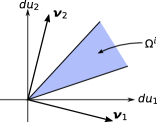
Figure 6: Example in which neither of the basis vectors of the null space (vectors $\boldsymbol{\nu}_{1}$ and $\boldsymbol{\nu}_{2}$) lies within the convex region $\Omega^{i}$, but a linear combination of the vectors would lie within $\Omega^{i}$.

One must, therefore, check the full sub-space spanned by the basis vectors. Although Farkas’ lemma might provide an elegant means of determining whether the sub-space intersects $\Omega^{i}$ (thus indicating the existence of a legitimate null-vector), in the examples of Section 4 we used a brute-force approach: we maximized the smallest element-wise product $\mathfrak{s}_{i}s_{i}$ in Eq. (88) and tested whether the largest product was positive (the search was made on the unit cube $[-1,1]^{m}$, where $m$ is the dimension of the null-space).

Another difficulty can arise when the criteria of Eqs. (90)–(92) are applied to realistic irregular assemblies of particles (as with the simulation data of Section 4.3). When a time-stepping algorithm is used to adjust the particle positions, a granular system can momentarily pass through the condition of neutral equilibrium during a single time step, so that the determinant of Eq. (91) is non-zero at the beginning and end of the step, although the neutral equilibrium condition (and the possibility of uncontrollable loading) would occur within the step. In this situation, the condition of neutral equilibrium would not be recognized. In analyzing such numerical data, we tested the condition number of matrix $\mathbf{H}^{i}$ (i.e., the ratio of the largest and smallest singular values found in the decomposition $[\mathbf{H^{i}}]=[\mathbf{U}][\boldsymbol{\Sigma}][\mathbf{V}]$) to determine the near-singularity of $\mathbf{H}^{i}$. When a large condition number was detected, we applied the Eckart–Young–Mirsky principle to find the near-null space of $[\mathbf{H}^{i}]$, isolating those vectors within $[\mathbf{V}]$ that corresponded to the smallest singular values. These basis vectors were then tested for consistency with the domain $\Omega^{i}$.

We finish this section by noting differences between neutral equilibrium and the loss of rigidity [10, 11]. The analysis of rigidity (and the related conditions of force staticity or indeterminacy) are familiar to physicists and structural engineers, and the analysis treats a system as if it is composed of rigid components: for example, rigid particles with rolling but rigid, non-compliant contacts. A rigid system is one that precludes articulated displacement modes in which no resistive forces are mobilized among the components; similarly, a hyperstatic or indeterminate system is one that admits a space of non-unique contact forces to support a given set of external forces. These conditions are established by considering only the kinematics (rigidity) matrix $[\mathbf{B}]$ of Eq. (19) (or its transpose, the statics matrix $[\mathbf{A}]$ of Eq. 7) and apply when the null space of $[\mathbf{B}]$ exceeds 6 (the null space can be no smaller, since six modes of rigid translation and rotation produce no relative movements among the components). Loss of rigidity occurs when the null space of $[\mathbf{B}]$ exceeds 6, thus admitting articulated displacement modes. Rigidity depends entirely upon $[\mathbf{B}]$, which is computed for the undisplaced condition; whereas, neutral equilibrium (or bifurcation and instability, as described in the next sections) depends upon the full stiffness $[\mathbf{H}]$, which incorporates both contact and geometric stiffnesses. The mechanical stiffness $[\mathbf{H}^{\text{m}}]$ involves a product with the matrix $[\mathbf{B}]$ (see Eq. 24), so that the rank of $[\mathbf{H}^{\text{m}}]$ can not exceed the rank of $[\mathbf{B}]$. The geometric stiffnesses, however, are not directly computed as products with $[\mathbf{B}]$, so that loss of rigidity does not imply neutral equilibrium, since articulated modes can be resisted by alterations of the system’s geometry, even though these modes do not mobilize any of the contacts’ stiffnesses.

3.2 Bifurcation and path instability

Bifurcation, whether stable or unstable, is the existence of multiple displaced equilibrium paths that emanate from the current equilibrium state for the particular loading increment $[d\boldsymbol{\mathfrak{p}}]$. Unlike neutral equilibrium (Section 3.1) and instability of an equilibrium state (Section 3.3), which are associated with a state, bifurcation involves a choice of equilibrium paths and is associated with a deformation process (path): bifurcation is a condition of path rather than state [22]. Another difference from neutral equilibrium is that the stiffness matrix at incipient bifurcation retains full rank, and the multiple solutions of Eq. (89) are for different stiffness branches $[\mathbf{H}^{i}]$, each with a direction $[d\mathbf{x}]$ that lies within its separate domain $\Omega^{i}$. The canonical example is the Shanley column, for which increased loading — rather than neutral loading — can occur along multiple bifurcation branches and for which states along each branch exhibit stability of equilibrium (see [38] and [25], which includes the succinct discussion of von Kármán).

Ignoring, for the moment, any constraints on displacement, bifurcation along a loading path $[d\boldsymbol{\mathfrak{p}}]$ is defined as the existence of multiple solutions, say “a” and “b” solutions, each lying within a separate stiffness domain:

$$\exists\left[d\mathbf{x}^{a}\right]\in\Omega^{a},\;\left[d\mathbf{x}^{b}\right]\in\Omega^{b},\;\Omega^{a}\neq\Omega^{b}:\quad\left[\mathbf{H}^{a}\right]\left[d\mathbf{x}^{a}\right]=\left[\mathbf{H}^{b}\right]\left[d\mathbf{x}^{b}\right]=\left[d\boldsymbol{\mathfrak{p}}\right]$$ (93)

Contrarily, a sufficient (but not necessary) condition for the uniqueness of a solution $[d\mathbf{x}^{0}]\in\Omega^{0}$ is the Hill condition

$$\left(\left[\mathbf{H}\right]\left[d\mathbf{x}\right]-\left[\mathbf{H}^{0}\right]\left[d\mathbf{x}^{0}\right]\right)^{\text{T}}\left(\left[d\mathbf{x}\right]-\left[d\mathbf{x}^{0}\right]\right)>0,\quad\forall\,\Omega^{i},\;\forall\,\left[d\mathbf{x}\right]\in\Omega^{i},\left[d\mathbf{x}\right]\neq\left[d\mathbf{x}^{0}\right]$$ (94)

that is, a positive value is found for all $[d\mathbf{x}]$ that are consistent with the prescribed loading increments $[d\boldsymbol{\mathfrak{p}}]$, such that $[\mathbf{H}][d\mathbf{x}]=[d\boldsymbol{\mathfrak{p}}]$ (see [26, 39, 22]).

Table 2 presents the bifurcation criterion of Eq. (93) in the contexts of the four types of displacement constraints in Section 2.4. With Type I constraint, we must check consistency with a domain $\Omega^{i}$ by reshuffling the constrained displacements $[d\mathbf{x}^{\text{c}}]$ into the solved displacements $[d\mathbf{x}^{\text{f}}]$. This difficulty is avoided with the other constraint types.

When multiple equilibrium solutions exist, one should then determine which of the alternative solutions is followed as the more stable path. Bažant [21, 40] addressed this issue by deriving the increments of internal entropy along each solution path of the external force $[d\mathbf{p}]$ and its associated movement $[d\mathbf{x}]$ — an increase $\Delta S_{\text{in}}$ that resembles the incremental form $[d\mathbf{p}]^{\text{T}}[d\mathbf{x}]$ of the second-order external work $\mathcal{B}_{2}$ in Eq. (53). However, Bažant noted that components of the vectors $[d\mathbf{x}]$ and $[d\mathbf{p}]$ must be treated differently for the separate cases of controlled movements and of controlled forces: (1) for those movements that are controlled, the subset $[d\mathbf{x}^{\text{c}}]$ is paired with the multiple sets of complementary restraining forces $[d\mathbf{p}^{\text{c},\alpha}]$ along the alternative $\alpha$-branches; and (2) for those external forces that are controlled, the subset $[d\mathbf{p}^{\text{f}\,}]$ is paired with the complementary solution movements $[d\mathbf{x}^{\text{f},\alpha}]$ along the alternative $\alpha$-branches. With this understanding, the second-order quantity

$$\mathcal{I}_{2}(d\mathbf{x}^{\alpha})=\frac{1}{2}\left(\left[d\mathbf{p}^{\text{c},\alpha}\right]^{\text{T}}\left[d\mathbf{x}^{\text{c}}\right]-\left[d\mathbf{p}^{\text{f}}\right]^{\text{T}}\left[d\mathbf{x}^{\text{f},\alpha}\right]\right)$$ (95)

can be computed for each $\alpha$ branch (a similar quantity was introduced by Hill [39] in developing stability extremum principles in a continuum setting). Bažant hypothesized that the system approaches equilibrium along the branch that maximizes $\mathcal{I}_{2}$. Petryk [22], also using energy arguments, defined a stable path as a branch $[d\mathbf{x}^{0}]\in A$ that satisfies the condition

$$\mathcal{I}_{2}(d\mathbf{x}^{0})\geq\mathcal{I}_{2}(d\mathbf{x}^{\alpha}),\quad\forall\left[d\mathbf{x}^{\alpha}\right]\in A$$ (96)

for the set $A$ of bifurcation paths, $A=\{[d\mathbf{x}^{a}],[d\mathbf{x}^{b}],[d\mathbf{x}^{0}],\ldots\}$, that satisfy Eq. (93). Contrarily, an unstable path $[d\mathbf{x}^{0}]\in A$, exhibiting path instability, is one for which

$$\exists\,[d\mathbf{x}^{\alpha}]\in A,\quad\mathcal{I}_{2}(d\mathbf{x}^{\alpha})>\mathcal{I}_{2}(d\mathbf{x}^{0})$$ (97)

An example is the Shanley column with an elasto-plastic hinge, for which three branches apply. In this case, an elasto-plastic column that is loaded to the tangent limit can remain straight with continued loading $d\mathbf{p}$ (i.e., the fundamental deformation $d\mathbf{x}^{0}$), or the column can buckle to the left or to the right. The fundamental deformation exhibits path instability, as the column is inclined to buckle by the criterion of Eq. (97).

In Table 2, the generic definition of path instability in Eq. (97) is given in the context of the four types of displacement constraints that were described in Section 2.4.

Table 2: Bifurcation with four types of displacement constraints and the corresponding definitions of path stability.

Generic bifurcation (without considering constraints, Eq. 93)

$\exists\,[d\mathbf{x}^{a}]\in\Omega^{a},\,[d\mathbf{x}^{a}]\in\Omega^{a},\,\Omega^{a}\neq\Omega^{b}:\;\;[\mathbf{H}^{a}][d\mathbf{x}^{a}]=[\mathbf{H}^{b}][d\mathbf{x}^{b}]=[d\mathbf{p}]$

Path stability, $\mathcal{I}_{2}(d\mathbf{x}^{\alpha})=\tfrac{1}{2}\left([d\mathbf{p}^{\text{c},\alpha}]^{\text{T}}[d\mathbf{x}^{\text{c}}]-[d\mathbf{p}^{\text{f}}]^{\text{T}}[d\mathbf{x}^{\text{f},\alpha}]\right)$:§

$\mathcal{I}_{2}(d\mathbf{x}^{0})\geq\mathcal{I}_{2}(d\mathbf{x}^{\alpha}),\forall[d\mathbf{x}^{\alpha}]\in A$

Type I constraint

Bifurcation

$\exists\,[d\mathbf{x}^{\text{c}}\times d\mathbf{x}^{\text{f},a}]\in\Omega^{a},[d\mathbf{x}^{\text{c}}\times d\mathbf{x}^{\text{f},b}]\in\Omega^{b},\Omega^{a}\neq\Omega^{b}$:

$[\mathbf{U}^{a}][d\boldsymbol{\mathfrak{p}}^{\text{c}}/d\mathbf{x}^{\text{f},a}]=[\mathbf{V}^{a}][d\mathbf{x}^{\text{c}}/d\boldsymbol{\mathfrak{p}}^{\text{f}\,}],\;[\mathbf{U}^{b}][d\boldsymbol{\mathfrak{p}}^{\text{c}}/d\mathbf{x}^{\text{f},b}]=[\mathbf{V}^{b}][d\mathbf{x}^{\text{c}}/d\boldsymbol{\mathfrak{p}}^{\text{f}\,}]$

Path stability of $[d\mathbf{x}^{0}]$, $\mathcal{I}_{2}(d\mathbf{x}^{a})=\frac{1}{2}[d\mathbf{x}^{\text{c}}/(-d\boldsymbol{\mathfrak{p}}^{\text{f}})]^{\text{T}}[\mathbf{U}^{a}]^{-1}[\mathbf{V}^{a}][d\mathbf{x}^{\text{c}}/d\boldsymbol{\mathfrak{p}}^{\text{f}\,}]$:§

$\mathcal{I}_{2}(d\mathbf{x}^{0})\geq\mathcal{I}_{2}(d\mathbf{x}^{\alpha}),\;\forall[d\mathbf{x}^{\alpha}]\in A_{\mathbf{x}}$

Type II constraint, $[\mathbf{X}^{i}]=[\mathbf{H}^{i}][\mathbf{P}_{\mathcal{L}}]+[\mathbf{P}_{\mathcal{L}^{\perp}}]$

Bifurcation:

$\exists\,[d\mathbf{z}^{a}],\;[d\mathbf{z}^{b}],\;[\mathbf{P}_{\mathcal{L}}][d\mathbf{z}^{a}]\in\Omega^{a},\;[\mathbf{P}_{\mathcal{L}}][d\mathbf{z}^{b}]\in\Omega^{b},\;\Omega^{a}\neq\Omega^{b}:\;\;$

$[\mathbf{X}^{a}][d\mathbf{z}^{a}]=[\mathbf{X}^{b}][d\mathbf{z}^{b}]=[d\boldsymbol{\mathfrak{p}}]$

Path stability of $[d\mathbf{z}^{0}]$, $\mathcal{I}_{2}(d\mathbf{z}^{\text{a}})=\tfrac{1}{2}\left([d\mathbf{y}^{\text{a}}]^{\text{T}}[d\mathbf{x}^{\text{a}}]-[d\boldsymbol{\mathfrak{p}}]^{\text{T}}[d\mathbf{x}^{\text{a}}]\right)$:∗∗,§

$\mathcal{I}_{2}(d\mathbf{z}^{0})\geq\mathcal{I}_{2}(d\mathbf{z}^{\alpha}),\;\forall[d\mathbf{z}^{\alpha}]\in A_{\mathbf{x}}$

Type III constraint, $[\mathbf{X}^{i}]=[\mathbf{H}^{i}][\mathbf{P}_{\mathcal{L}}]+[\mathbf{P}_{\mathcal{L}^{\perp}}]$, $[d\boldsymbol{\mathfrak{y}}^{i}]=[\mathbf{H}^{i}][\mathbf{C}]^{\dagger}[d\mathbf{c}]$

Bifurcation:∗

$\exists\,[d\mathbf{z}^{a}],\;[d\mathbf{z}^{b}],\;[\mathbf{C}]^{\dagger}[d\mathbf{c}]+[\mathbf{P}_{\mathcal{L}}][d\mathbf{z}^{a}]\in\Omega^{a},\;[\mathbf{C}]^{\dagger}[d\mathbf{c}]+[\mathbf{P}_{\mathcal{L}}][d\mathbf{z}^{b}]\in\Omega^{b},\;\Omega^{a}\neq\Omega^{b}:\;\;$

$[\mathbf{X}^{a}][d\mathbf{z}^{a}]=[d\boldsymbol{\mathfrak{p}}]-[d\boldsymbol{\mathfrak{y}}^{a}],\;[\mathbf{X}^{b}][d\mathbf{z}^{b}]=[d\boldsymbol{\mathfrak{p}}]-[d\boldsymbol{\mathfrak{y}}^{b}]$

Path stability of $[d\mathbf{z}^{0}]$, $\mathcal{I}_{2}(d\mathbf{z}^{\text{a}})=\frac{1}{2}\left([d\mathbf{y}^{\text{a}}]^{\text{T}}[d\mathbf{x}^{\text{a}}]-[d\boldsymbol{\mathfrak{p}}]^{\text{T}}[d\mathbf{x}^{\text{a}}]\right)$:${}^{\rule{0.90417pt}{0.0pt}\ast\ast,\S}$

$\mathcal{I}_{2}(d\mathbf{z}^{0})\geq\mathcal{I}_{2}(d\mathbf{z}^{\alpha}),\;\forall[d\mathbf{z}^{\alpha}]\in A_{\mathbf{x}}$

Type IV constraint, $[\mathbf{X}^{i}]=[\mathbf{H}^{i}][\mathbf{P}^{\text{n-r-r}}]+[\mathbf{P}^{\text{r-r}}]$

Bifurcation:

$\exists\,[d\mathbf{z}^{a}],\;[d\mathbf{z}^{b}],\;[\mathbf{P}^{\text{n-r-r}}][d\mathbf{z}^{a}]\in\Omega^{a},\;[\mathbf{P}^{\text{n-r-r}}][d\mathbf{z}^{b}]\in\Omega^{b},\;\Omega^{a}\neq\Omega^{b}:\;\;$

$[\mathbf{X}^{a}][d\mathbf{z}^{a}]=[\mathbf{X}^{b}][d\mathbf{z}^{b}]=[d\boldsymbol{\mathfrak{p}}]$

Path stability of $[d\mathbf{z}^{0}]$, $\mathcal{I}_{2}(d\mathbf{z}^{\text{a}})=\tfrac{1}{2}\left([d\mathbf{y}^{\text{a}}]^{\text{T}}[d\mathbf{x}^{\text{a}}]-[d\boldsymbol{\mathfrak{p}}]^{\text{T}}[d\mathbf{x}^{\text{a}}]\right)$:‡,§

$\mathcal{I}_{2}(d\mathbf{z}^{0})\geq\mathcal{I}_{2}(d\mathbf{z}^{\alpha}),\;\forall[d\mathbf{z}^{\alpha}]\in A_{\mathbf{x}}$

∗ $[d\boldsymbol{\mathfrak{y}}^{a}]=[\mathbf{H}^{a}][\mathbf{C}]^{\dagger}[d\mathbf{c}]$

∗∗ $[d\mathbf{y}^{\alpha}]=-[d\boldsymbol{\mathfrak{p}}]+[\mathbf{H}^{\alpha}][d\mathbf{x}^{\alpha}]$, $[d\mathbf{x}^{\alpha}]=[\mathbf{P}_{\mathcal{L}}][d\mathbf{z}^{\alpha}]$

‡ $[d\mathbf{y}^{\alpha}]=-[d\boldsymbol{\mathfrak{p}}]+[\mathbf{H}^{\alpha}][d\mathbf{x}^{\alpha}]$, $[d\mathbf{x}^{\alpha}]=[\mathbf{P}^{\text{n-r-r}}][d\mathbf{z}^{\alpha}]$

§ $A_{\mathbf{x}}=\{[d\mathbf{x}^{a}],[d\mathbf{x}^{b}],[d\mathbf{x}^{0}],\ldots\}$, the set of all solutions

With simple Type I constraint, the $\alpha$-branch is the mixed solution of Eq. (55), $[d\boldsymbol{\mathfrak{p}}^{\text{c}}/d\mathbf{x}^{\text{f}}]=[\mathbf{U}^{\alpha}]^{-1}[\mathbf{V}^{\alpha}][d\mathbf{x}^{\text{c}}/d\boldsymbol{\mathfrak{p}}^{\text{f}}]$, and the second-order quantity $\mathcal{I}_{2}(d\mathbf{x}^{\alpha})$ is the product $[d\mathbf{x}^{\text{c}}/(-d\boldsymbol{\mathfrak{p}}^{\text{f}})][\mathbf{U}^{\alpha}]^{-1}[\mathbf{V}^{\alpha}][d\mathbf{x}^{\text{c}}/d\boldsymbol{\mathfrak{p}}^{\text{f}}]$, noting the negative sub-vector $[-d\boldsymbol{\mathfrak{p}}^{\text{f}}]$, as in Eq. (95). With Type II and III constraints, the term $[d\mathbf{p}^{\text{f}}]^{\text{T}}[d\mathbf{x}^{\text{f},\alpha}]$ in Eq. (95) is the product of the vectors $[d\boldsymbol{\mathfrak{p}}]$ and $[d\mathbf{x}]$ that appear in Eqs. (62) and (69); whereas the term $[d\mathbf{p}^{\text{c},\alpha}]^{\text{T}}[d\mathbf{x}^{\text{c}}]$ is the product of the reaction forces $[d\mathbf{y}]$ and the movements $[d\mathbf{x}]$, as in Eqs. (62), (69), and (70). Type IV constraint is analyzed in a similar manner, with the projection matrix $[\mathbf{P}^{\text{n-r-r}}]$ taking the place of matrix $[\mathbf{P}_{\mathcal{L}}]$ in computing vectors $[d\boldsymbol{\mathfrak{p}}]$ and $[d\mathbf{x}]$.

3.3 Instability of equilibrium

With instability of equilibrium, an impulsive departure from an equilibrium state is energetically available without a change in the loading parameters. Eq. (49) of Section 2.3 gives the rate of kinetic energy $\ddot{E}$ (or rate of internal entropy) for an equilibrium system perturbed across a time span of $\Delta t$ by the rates of movement and loading, $[\dot{\mathbf{x}}]$ and $[\dot{\mathbf{q}}]$. If the loading rate $[\dot{\mathbf{q}}]$ is suspended at a particular state (i.e., is momentarily zero), so that $\mathcal{B}_{2}=0$, a spontaneous increase in $E$ is energetically favored when the second-order work $\mathcal{W}_{2}$ is negative in a particular movement direction of $[\dot{\mathbf{x}}]$. Because this movement must be consistent with the directional stiffness $[\mathbf{H}^{i}]$, instability of equilibrium is defined as

$$\exists\left[d\mathbf{x}\right]\in\Omega^{i}:\;\;\left[d\mathbf{x}\right]^{\text{T}}\left[\mathbf{H}^{i}\right]\left[d\mathbf{x}\right]<0$$ (98)

(note that this definition is generic, as we have not yet considered any movement constraints). Even with a non-vanishing loading rate, $[\dot{\mathbf{q}}]\neq 0$, such that $\mathcal{B}_{2}(\dot{\mathbf{x}})\neq 0$, the rate $\ddot{E}$ in Eq. (49) is dominated by $\mathcal{W}_{2}$, which is quadratic in $[d\mathbf{x}]$, so that $[d\mathbf{q}]$, in principle, can be treated as zero.

Because Eq. (98) involves a scalar quadratic form, an alternative definition of instability of equilibrium is the existence of a stiffness matrix $[\mathbf{H}^{i}]$ with a negative eigenvalue of its symmetric part, $[\widehat{\mathbf{H}}^{i}]=\tfrac{1}{2}([\mathbf{H}^{i}]+[\mathbf{H}^{i}]^{\text{T}})$, for which the corresponding eigenvector lies within $\Omega^{i}$. Similar to Eq. (92), we designate $\{\lambda([\widehat{\mathbf{Z}}])\}$ as the set of eigenvalues of the symmetric matrix $[\widehat{\mathbf{Z}}]$, and $\{\boldsymbol{\eta}_{-}([\widehat{\mathbf{Z}}])\}$ as the subspace spanned by those eigenvectors corresponding to the negative eigenvalues of the symmetric part. An alternative (generic) definition of instability of equilibrium is

$$\exists\left[\mathbf{H}^{i}\right]:\;\;\{\lambda([\widehat{\mathbf{H}^{i}}]):\lambda<0\}\neq\varnothing,\;\{\boldsymbol{\eta}_{-}([\widehat{\mathbf{H}^{i}}])\}\cap\Omega^{i}\neq[\mathbf{0}]$$ (99)

The above two definitions are closely related to the concept of unsustainability proposed by Nicot and Darve [3]. In a continuum setting, unsustainablity arises when a change in the stress and strain of a region can be reached through a dynamic process without any change in control parameters applied to the region’s boundary and interior. In a discrete setting, this condition is equivalent to the generic criterion $\mathcal{W}_{2}(\dot{\mathbf{x}})<0$ of Eqs. (98)–(99), noting that notions of “boundary” and “interior” are to be avoided with discrete systems. We also note that stability criteria in Eqs. (98) and (99) are restricted to a quasi-static setting, in which the system is initially in stationary equilibrium (Section 2.3). It is possible to show, for instance, that in a full dynamic setting, flutter can arise in non-conservative systems before a mode of negative second-order work is available [24].

Much attention has been given to the hierarchy of the different pathologies, in particular to the question of whether instability of equilibrium precedes neutral equilibrium. Such hierarchy is based upon the following matrix property: the real parts of the eigenvalues of a matrix $[\mathbf{H}]$ are bounded by the smallest and largest eigenvalues of its symmetric counterpart,

$$\text{min}\,\{\lambda([\widehat{\mathbf{H}}])\}\leq\{\text{Re}\left(\lambda([\mathbf{H}])\right)\}\leq\text{max}\,\{\lambda([\widehat{\mathbf{H}}])\}$$ (100)

As such, for elastic systems that undergo a smooth, continuous transition of stiffness during a loading program, instability of equilibrium is encountered before neutral equilibrium: a negative eigenvalue of the symmetric matrix $[\widehat{\mathbf{H}}]$ is encountered before a zero eigenvalue appears (along with a zero determinant) with the full matrix $[\mathbf{H}]$. For a smooth stiffness operator, Challamel et al. [24] have shown that the second-order work criterion for a non-conservative system coincides with neutral equilibrium with one homogeneous (i.e., Type II) constraint, and Lerbet et al. [41] have generalized this result to systems with $n$ constraints. This hierarchy of second-order work and neutral equilibrium does not necessarily apply to non-smooth inelastic systems. The eigenvectors of the full stiffness matrix and of its symmetric counterpart are not equal, and it is possible that the negative eigenvalues of the symmetric stiffness $[\widehat{\mathbf{H}}^{i}]$ correspond to eigenvectors that lie outside the stiffness’s domain $\Omega^{i}$; whereas, the full matrix $[\mathbf{H}^{i}]$ can have a zero eigenvalue with a different eigenvector, but one that lies within $\Omega^{i}$.

Table 3 places these generic definitions of instability of equilibrium in the context of the four types of movement constraints described in Section 2.4.

Table 3: Instability of equilibrium with four types of displacement constraints.

Generic instability of equilibrium (without considering constraints, Eqs. 98–99)
a)	$\exists\,[d\mathbf{x}]\in\Omega^{i}:\;\;[d\mathbf{x}]^{\text{T}}[\mathbf{H}^{i}][d\mathbf{x}]<0$
b)	$\exists\,[\mathbf{H}^{i}]:\;\;\{\lambda([\widehat{\mathbf{H}^{i}}])\!:\lambda<0\}\neq\varnothing,\;\{\boldsymbol{\eta}_{-}([\widehat{\mathbf{H}^{i}}])\}\cap\Omega^{i}\neq[\mathbf{0}]$
Type I constraint
a)	$\exists\,[d\mathbf{x}]=[d\mathbf{x}^{\text{c}}/d\mathbf{x}^{\text{f}\,}]\in\Omega^{i}:\;\;[d\mathbf{x}^{\text{f}\,}]^{\text{T}}[\mathbf{H}^{\text{f{}f},i}][d\mathbf{x}^{\text{f}\,}]<0$
b)	$\exists\,[\mathbf{H}^{i}]:\;\;\{\lambda([\widehat{\mathbf{H}^{\text{f{}f},i}}])\!:\lambda<0\}\neq\varnothing,\;\left([d\mathbf{x}^{\text{c}}]\times\{\boldsymbol{\eta}_{-}([\widehat{\mathbf{H}^{\text{f{}f},i}}])\}\right)\cap\Omega^{i}\neq[\mathbf{0}]$
Types II and III constraints
a)	$\exists\,[d\mathbf{z}],\;[\mathbf{P}_{\mathcal{L}}][d\mathbf{z}]\in\Omega^{i}:\;\;[d\mathbf{z}]^{\text{T}}\left([\mathbf{P}_{\mathcal{L}}]^{\text{T}}[\mathbf{H}^{i}][\mathbf{P}_{\mathcal{L}}]\right)[d\mathbf{z}]<0$
b)	$\exists\,[\mathbf{H}^{i}]:\;\;\left\{\lambda\!\left([\mathbf{P}_{\mathcal{L}}]^{\text{T}}[\widehat{\mathbf{H}^{i}}][\mathbf{P}_{\mathcal{L}}]\right)\!:\lambda<0\right\}\neq\varnothing,\;\left\{\boldsymbol{\eta}_{-}\!\left([\mathbf{P}_{\mathcal{L}}]^{\text{T}}[\widehat{\mathbf{H}^{i}}][\mathbf{P}_{\mathcal{L}}]\right)\right\}\cap\Omega^{i}\neq[\mathbf{0}]$
Type IV constraint
a)	$\exists\,[d\mathbf{z}],\;[\mathbf{P}_{\mathcal{L}}][d\mathbf{z}]\in\Omega^{i}:\;\;[d\mathbf{z}]^{\text{T}}\left([\mathbf{P}^{\text{n-r-r}}]^{\text{T}}[\mathbf{H}^{i}][\mathbf{P}^{\text{n-r-r}}]\right)[d\mathbf{z}]<0$
b)	$\exists\,[\mathbf{H}^{i}]:\;\;\left\{\lambda\!\left([\mathbf{P}^{\text{n-r-r}}]^{\text{T}}[\widehat{\mathbf{H}^{i}}][\mathbf{P}^{\text{n-r-r}}]\right)\!:\lambda<0\right\}\neq\varnothing,\;\left\{\boldsymbol{\eta}_{-}\!\left([\mathbf{P}^{\text{n-r-r}}]^{\text{T}}[\widehat{\mathbf{H}^{i}}][\mathbf{P}^{\text{n-r-r}}]\right)\right\}\cap\Omega^{i}\neq[\mathbf{0}]$

For example, with Type I constraint, the known, constrained displacements $[d\mathbf{x}^{\text{c}}]$ are treated as zero, since the quadratic form of Eq. (98) is dominated by the product $[d\mathbf{x}^{\text{f}\,}]^{\text{T}}[\mathbf{H}^{\text{f{}f},i}][d\mathbf{x}^{\text{f}\,}]$. Restricting the question of instability to a test of whether the submatrix $[\mathbf{H}^{\text{f{}f},i}]$ is semi-definite or indefinite reduces the displacement-space that is available for instability modes from $\mathbb{R}^{6N}$ to $\mathbb{R}^{6N-r}$ (recall that $r$ displacements are constrained). Similarly, with Types II and  III constraints, one need not query the full space $[d\mathbf{z}]\in\mathbb{R}^{6N}$; rather, one must only consider the projection $[\mathbf{P}_{\mathcal{L}}][d\mathbf{z}]$ of $\mathbb{R}^{6N}$ onto the subspace $\mathcal{L}$ that satisfies the displacement constraints (Eqs. 57 and 64). With Type IV constraint, we are only concerned with instability associated with particle motions that are not rigid-body movements of the entire assembly, and by investigating the product $[\mathbf{P}^{\text{n-r-r}}]^{\text{T}}[\widehat{\mathbf{H}^{i}}][\mathbf{P}^{\text{n-r-r}}]$ we eliminate any second-order work that is merely an artifact of the rigid rotation of the assembly and its external forces.

Finally, we note that a numerical search for modes of unstable equilibrium can encounter the same difficulties faced in determining neutral equilibrium, as were discussed and resolved in the final two paragraphs of Section 3.1.

4 Examples

We now consider three examples of increasing complexity, involving three, twelve, and sixty-for disks. In each example, we identify multiple (sometimes thousands of) stiffness pathologies. Of the several criteria for distinguishing neutral equilibrium and instability of equilibrium, we applied the particular criteria of Eqs. (91) and (99). For these two-dimensional situations, the curvature tensors $[\mathbf{K}^{pq,p}]$ and $[\mathbf{K}^{pq,q}]$ are simplified as $-(1/\rho^{p})[\mathbf{n}^{pq}]^{\text{T}}[\mathbf{n}^{pq}]$ and $-(1/\rho^{q})[\mathbf{n}^{pq}]^{\text{T}}[\mathbf{n}^{pq}]$, where $\rho^{p}$ and $\rho^{q}$ are the particles’ radii of curvature at the contact point $pq$. Each example was numerically analyzed with Matlab code.

4.1 Example 1: three disks

In this simplest example, we examine a system of three disks (Fig. 7).

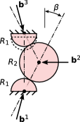
Figure 7: Example 1: three disks, in which the two contacts are at the friction limit. Rotation and horizontal movement is prevented with the top and bottom disks, while the top disk is displaced downward.

The top and bottom disks have the same radius $R_{1}$ and are centered on a vertical line; whereas, the middle disk has radius $R_{2}$ and is offset by angle $\beta$ from the top and bottom disks. The two contacts share the same contacts stiffness and friction coefficient (values $k=1$, $\alpha=1$, and $\mu=0.5$). The top and bottom disks are not allowed to rotate or to move horizontally, and the bottom disk is constrained from vertical movement. The three disks touch at two contacts with an equal normal contact force of 0.001$k$, and both contacts are assumed at the friction limit, with the directions of their tangential force being consistent with a vertical compression of the assembly. The system is loaded by displacing the top disk downward toward the bottom disk (i.e., $\dot{u}_{2}^{3}<0$). Briefly, the non-rotating top and bottom disks are pressed vertically upon the middle disk and a constant force $\mathbf{b}^{2}$ places the two contacts at the friction limit. The system has only four kinematic degrees of freedom ($u_{2}^{1}$, $u_{2}^{2}$, $\theta_{3}^{2}$, and $u_{2}^{3}$), with five forces of constraint (the reactions $b_{1}^{1}$, $b_{2}^{1}$, $w_{3}^{1}$, $b_{1}^{3}$, and $w_{3}^{3}$).

We consider three relative radii of the disks ($R_{2}<R_{1}$, $R_{2}=R_{1}$, and $R_{2}>R_{1}$), and three relative offset angles $\beta$. When $\beta=\cot(\mu)$, the top and bottom external forces, $\mathbf{b}^{1}$ and $\mathbf{b}^{3}$, are vertical, and no external force acts upon the middle particle ($\mathbf{b}^{2}=\mathbf{0}$); however, when $\beta$ is less than (greater than) $\cot(\mu)$, equilibrium requires that the external forces $\mathbf{b}^{1}$ and $\mathbf{b}^{3}$ must have a leftward (rightward) component, and the external force $\mathbf{b}^{2}$ must have a rightward (leftward) component, so that the two contacts are held at the friction limit. Figure 7 depicts the case of $R_{2}>R_{1}$ and $\beta<\cot(\mu)$, with $\mathbf{b}^{2}$ acting toward the left.

Although this three-disk assembly seems fairly simple, it displays several pathologies, which are summarized in Table 4.

Table 4: Stiffness pathologies of the three-disk system in Fig. 7, in which the contacts’ radii of curvature are the same as the disks’ physical radii ($\rho=R$). Each $\Box$ indicates a solution of the stiffness problem, with multiple $\Box$’s representing a bifurcation. Each $\triangle$ indicates an instability of equilibrium, with multiple $\triangle$’s representing multiple unstable modes. A $\boxtimes$ means that no solution exists.

	$R_{2}<R_{1}$	$R_{2}=R_{1}$	$R_{2}>R_{1}$
$\beta<\cot(\mu)$	$\square\square$	$\square\square$	$\square\square$
$\beta=\cot(\mu)$	$\boxtimes$	$\boxtimes$	$\boxtimes$
	$\triangle$	$\triangle$	$\triangle\triangle\triangle$
$\beta>\cot(\mu)$	$\square\square\square$	$\square\square\square$	$\square\square\square$
	$\triangle$	$\triangle$	$\triangle\triangle\triangle$

Because both contacts are at the friction limit, we must investigate $2^{2}=4$ possible slip (or no-slip) combinations and check whether the displacement of the solutions (or pathologies) of each combination are consistent with the assumed slip (or no-slip) combination. As an example, when $\beta=\cot(\mu)$ (i.e., when the equilibrating side force $\mathbf{b}^{2}$ is zero), no solution exists that will maintain the constant, zero side force. Indeed,this arrangement places the system in an untenable, unstable condition, and the middle particle will squirt to the right without being prompted by any movement of the top and bottom particles: a negative second-order work is associated with both contacts during a horizontal movement of the middle disk. When the middle disk is larger than the top and bottom disks and $\beta=\cot(\mu)$, three instability modes are available: a mode whereby horizontal movement of the middle disk toward the right causing frictional slip of both contacts, and two modes in which only one contact slips while the middle disk both rotates and obliquely moves as it “escapes” from the other disks.

The case of $\beta>\cot(\mu)$ is also unusual, as three solutions are available, creating a possible trifurcation with path instability (i.e., the triplets of squares in the bottom of Table 4). Note that when $\beta>\cot(\mu)$, the external force $\mathbf{b}^{2}$ is pulling the middle disk toward the right to bring the two contacts to the friction limit. Each solution is along a different stiffness branch (i.e., with a different combination of slip and no-slip contacts). The first solution is a slight rightward movement of the middle disk, causing the two contacts to elastically unload with no slip. The other two solutions involve one slipping contact and one elastic contact and a rotation and rightward movement of the middle disk. Of the three solutions, the first solution is the more stable, with the largest $\mathcal{I}_{2}(d\mathbf{x}^{\alpha})$ value. But even this solution branch is unstable, since a rightward movement of the middle disk in the absence of movements of the top and bottom disks will exhibit negative second-order work with frictional slip in both contacts (the triangles in the bottom row of the table).

We now consider the extent to which geometric effects are manifested in this simple system, which we illustrate in two ways. Equation (37) gives the stiffness as a sum of mechanical and geometric parts, $[\mathbf{H}^{\text{m}}]$ and $[\mathbf{H}^{\text{g}}]$. The results of our analysis are quite different when the geometric stiffness is ignored and only the mechanical stiffness is considered. For example, neutral equilibrium would be predicted in each of the $\beta=\cot(\mu)$ cases reported in Table 4. Neglecting the geometric stiffness, no rotation of the contact forces would occur during a vertical movement of both the top and bottom particles, and no change in the $\mathbf{b}^{2}$ force would be predicted: that is, the vector $[\mathbf{p}]$ in Eq. (90) would be zero, indicating neutral equilibrium. This result is corrected with the inclusion of the $[\mathbf{H}^{\text{g}}]$ stiffness.

Another illustration of geometric effects is presented in Table 5.

Table 5: Stiffness pathologies of a three-disk system. Unlike Fig. 7 and Table 4, the radii of curvature are increased by a factor of 2 at the contact points, $\rho=2R$. Each $\Box$ indicates a solution of the stiffness problem, with multiple $\Box$’s representing a bifurcation. Each $\triangle$ indicates an instability of equilibrium, with multiple $\triangle$’s representing multiple unstable modes. A $\boxtimes$ means that no solution exists. Solutions with symbol “$\boxminus$” differ from those in Table 4.

	$R_{2}<R_{1}$	$R_{2}=R_{1}$	$R_{2}>R_{1}$
$\beta<\cot(\mu)$	$\boxminus$	$\boxminus$	$\boxminus$
$\beta=\cot(\mu)$	$\boxtimes$	$\boxtimes$	$\boxtimes$
	$\triangle$	$\triangle$	$\triangle\triangle\triangle$
$\beta>\cot(\mu)$	$\square\,\boxminus$	$\square\,\boxminus$	$\square\,\boxminus$
	$\triangle$	$\triangle$	$\triangle\triangle\triangle$

This table is for a three-disk system in which the shapes of the particles have been altered at the contact points. Here, the particles have the radii $R_{1}$ and $R_{2}$, but at their points of contact, we have slightly “flattened” the particles’ contours by artificially increasing their radii of curvature by a factor of 2. The amended results in Table 5 can be compared with those of Table 4, in which the particles’ radii of curvature are equal the disks’ bulk curvature. The numbers of solutions, designated with squares in the tables, are different for the cases of $\rho=R$ and $\rho=2R$, and solutions in Table 5 that are marked as “$\boxminus$” occur with a different combination of slip/no-slip contacts than those in Table 4. The subtle geometry of the particles’ contacts clearly affect the assembly’s stiffness and the solutions of a displacement problem.

4.2 Example 2: regular array of twelve disks

The second example involves a regular arrangement of twelve equal-size disks (Fig. 8).

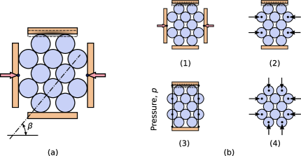
Figure 8: (a) regular array of twelve disks examined in Example 2, with each disk-disk contact at the friction limit. (b) Four different boundary types are considered. With the first three boundary types, the top and bottom platens are displaced vertically toward each other.

Four different problems are investigated, each with its own types of boundaries: (1) four platens that restrict the movements of the outer disks; (2) only top and bottom platens, with constant external forces applied to the side disks; (3) only top and bottom platens, with a flexible boundary along the side disks, applying a constant pressure; and (4) Type IV constraint with no displacement constraints applied to the particles. All disk-disk and disk-platen contacts share the same stiffness and friction coefficient (values $k=1$, $\alpha=1$, and $\mu=0.5$), and each contacting disk-disk pair has the same contact orientation $\beta$. All disk-disk contacts have an equal normal force of 0.001$k$, and all disk-disk contacts are placed at the friction limit, with the directions of their tangential force being consistent with a vertical compression of the assembly. Because of the symmetric disk arrangement, the disk-platen forces have no tangential component, so that equal vertical forces are applied at all top and bottom disk-platen contacts, and equal horizontal forces are applied at all side disk-platen contacts.

The first three problems include top and bottom platens, and these platens are constrained from moving horizontally and are vertically pressed toward (approaching) each other with a vertical displacement. These displacement conditions can be modeled as either Type I or Type III constraints. With the four-platen problem (problem 1), we include side platens but disallow their vertical movement, and a constant horizontal external forces $\mathbf{b}$ are applied to these side platens. The side platens are removed for problem 2, and their horizontal disk-platen contact forces are replaced with constant horizontal external forces $\mathbf{b}$, applied at the centers of the side particles. With problem 3, the horizontal external forces are produced by imaginary membranes (one membrane on the left, another membrane on the right) that are draped between the top and bottom platens and pass through the centers of the side particles. A constant pressure $p$ is applied to the membranes, sufficient to equilibrate the contact forces that act upon the side disks. The external forces applied by the membranes to the disks are position-dependent: the forces are altered by changes in the disk-disk and disk-platen distances, and their directions are altered by any relative shifting of the disks. That is, the membrane forces are position-dependent and involve introducing a $[\mathbf{H}^{\text{g-4}}]$ geometric stiffness. With problem 4, we remove all platens and membranes and treat the twelve disks as an isolated system.

There are 16 contacts among the twelve disks, and because each disk-disk contact is at the friction limit, we must search for stiffness pathologies among the $2^{16}=$ 65,536 possible combinations of slip and no-slip at the contacts. Results for the four problems are given in Table 6 for the case of $\beta=50^{\circ}$, for which the side particles (or platens) must press inward on the disks, to place each disk-disk contact at the friction limit.

Table 6: Stiffness pathologies of the twelve-disk systems in Fig. 8.

	Number of	Number of	Number of
	neutral modes	solutions	unstable modes
Problem 1: four platens	0	231	7,272
Problem 2: two platens, constant side forces	0	251	13,320
Problem 3: two platens, constant side pressure	0	70	13,247
Problem 4: isolated system	1	—	52,033

The assembly with four platens (problem 1) does not have a unique solution: there are 231 separate solutions, offering a multitude of bifurcation opportunities — a multi-furcation. Each of the solutions would produce slip at a subset of the contacts while producing elastic (no-slip) movements at the remaining contacts, and with each solution, the combination of contacts that are in a slip or no-slip condition is consistent with the particles’ movements (Section 2.6). Of the 231 solutions, 34 exhibit path stability, as the other solutions yield smaller values of $\mathcal{I}_{2}(d\mathbf{x}^{\alpha})$. The 34 stable solutions involve symmetric systems of rotations of the particles and platens and produce slip displacements at 8 of the 16 disk-disk contacts, while the other 8 contacts are displaced elastically. These 34 solutions produce the same displacements of the four platens. The other $231-34=197$ solutions are unstable bifurcation paths: even though they produce the same downward movement of the top platen, these modes have different movements of the side platens (i.e., different dilation rates).

However, even when all platens are stationary, the system is unstable, as the constrained stiffness $[\mathbf{H}]$ has 7272 branches (modes) that are unstable. This situation is not surprising, since each of the disk-disk contacts is initially loaded to the friction limit, and there are numerous opportunities for the spontaneous generation of negative second-order work by the shifting of particles. We also investigated a variation of problem 1, in which we disallowed rotations of the four platens. The numbers of solutions and unstable branches for problem 1 are greatly reduced when rotations of the platens are prevented. This additional constraint reduces the number of solutions to 118 and the number of unstable branches to 2460.

The other three problems in Fig. 8b have similar characteristics (see Table 6). The only example of neutral equilibrium, however, occurs with the isolated assembly of problem 4. In this problem, we applied no change of the external forces, such that $[d\mathbf{p}]=[\mathbf{0}]$, and the neutral, uncontrollable mode is simply the synchronized gear-like rotations of all 12 disks, in which each disk rolls against its neighbors but none of the gears are displaced. This rolling mode produces no changes in the contact forces and no change in the external forces. As such, any non-zero set of equilibrated force increments $[d\mathbf{p}]$ can be produced by a superposition of a set of disk movements and the gear-like mode.

4.3 Example 3: irregular assembly of 64 disks

An assembly of 64 particles was created and then loaded with the discrete element (DEM) finite-difference algorithm, and at particular stages of loading, the assembly’s condition was analyzed using the stiffness methods derived in the paper (Fig. 9).

Figure 9: Assembly of 64 disks that was created with a DEM simulation.

The DEM method applies Newton’s equations in a time-stepping algorithm to advance the particles’ positions, while maintaining near-equilibrium of the forces among particles and approximating the particles’ rearrangements. The particles are never in equilibrium, however, as the algorithm relies upon dis-equilibrium to impel particles to new locations. Therefore, questions of bifurcation and instability are not directly addressed with the DEM, as the particles’ inertias sweep them along a solution path, possibly passing through the various pathologies that were described in Section 3 and that would otherwise be confronted under true quasi-static loading conditions.

The irregular arrangement of the 64 disks was created by placing them sparsely within four flat platens, assigning the disks random velocities, and isotropically reducing the assembly dimensions. The average disk radius $D$ was about 0.5, and the largest disk was about 3 times larger than the smallest. All disk-disk and disk-platen contacts were assigned the same properties: $k=1$, $\alpha=1$, and $\mu=0.5$. Once compacted, the average contact force was about 0.0034$kD$. The assembly was then compressed in the vertical direction at a constant rate of strain while maintaining constant horizontal stress by adjusting the separation of the side platens. The deviator stress $q$ and vertical strain $\varepsilon_{22}$ are shown in Fig. 10 for this stage of biaxial compression.

Figure 10: Stress and strain from DEM simulation of biaxial compression of an irregular arrangement of 64 disks.

The ragged, serrated nature of the evolving stress is typical of DEM simulations of small assemblies and is also observed in laboratory tests of large specimens of glass beads [42, 43, 44]. We focus on a brief episode of strain “C”, located at the peak deviator stress which is circled in Fig. 10 and detailed in the inset figure. Other strains (”A”, ”B”, and ”D”) are considered near the end of this section.

At the peak stress “C”, we determined which stiffness pathologies were present with two types of boundaries. First, we analyzed the same conditions that were used in the DEM simulation: zero movement of the bottom platen, zero rotation of all four platens, constant horizontal stress on the two side platens, and a relative downward vertical movement of the top platen. To maintain constant horizontal stress, we introduced a geometric stiffness $[\mathbf{H}^{\text{g-4}}]$ that would reduce the horizontal forces on the side platens with a reduction in the assembly’s height. This first type of boundaries was analyzed using Type III constraint, although the same results would be found by applying Type I constraint. The second type of boundaries was simply Type IV constraint, in which we removed the platens and treated the disk assembly as an isolated system without any displacement constraints. This Type IV constraint is intended to capture the inherent material behavior in the absence of any restrictive boundaries that might suppress the onset of bifurcations or other stiffness pathologies.

A snapshot of the DEM data was taken at the peak deviator stress “C” (circled in Fig. 10), which included all particle positions and all contact forces and orientations. Of the original 68 particles (64 disks and 4 platens), seven disks were “rattler” particles having zero or one contacts with other disks, and these rattlers were ignored in the analysis and are not shown in Fig. 9. Because a DEM simulation merely approximates equilibrium, the contact forces in the snapshots were slightly out-of-equilibrium, with small but non-zero net forces and moments, $d\mathbf{b}^{p}$ and $d\mathbf{w}^{p}$, on the particles. The data was pre-conditioned to restore equilibrium by slightly adjusting the contact forces $\mathbf{f}^{pq}$ with small adjustments $d\mathbf{f}^{pq}$ by projecting the out-of-equilibrium forces $[d\mathbf{p}]=[d\mathbf{b}/d\mathbf{w}]$ onto the equilibrium sub-space given by the columns of the statics matrix $[\mathbf{A}]$ (see Eq. 7):

$$\left[\boldsymbol{\mathfrak{f}}\right]\leftarrow\left[\boldsymbol{\mathfrak{f}}\right]-[d\boldsymbol{\mathfrak{f}}],\quad\quad\left[d\boldsymbol{\mathfrak{f}}\right]=\left[\mathbf{A}]^{\dagger}[d\mathbf{p}\right]$$ (101)

where $[d\boldsymbol{\mathfrak{f}}]=[d\mathbf{f}/d\mathbf{m}]$, and $[\mathbf{A}]^{\dagger}$ is the Moore–Penrose inverse $[\mathbf{A}]^{\text{T}}([\mathbf{A}][\mathbf{A}]^{\text{T}})^{-1}$.

There were 97 contacts among the disks and platens at “C”, and because 14 of these contacts were at the friction limit, we searched for stiffness pathologies among the $2^{14}=$ 16,384 possible combinations of slip and no-slip at the 14 contacts. Our results show that only a single solution exists for the problem (i.e., no bifurcation of solutions), and this solution yielded platen movements that were similar to those found in the DEM simulation. No modes of neutral equilibrium were found, but the system exhibited 306 unstable modes. That is, if the platens’ movements were frozen, particle movements could spontaneously occur in 306 possible patterns. We also considered an assembly with the same arrangement of particles but without the four platens: a Type IV isolated system. By removing the platens and replacing them with external forces on the peripheral particles, the disks have more freedom, and the 306 unstable modes increased to 807.

The fact that this granular system can exhibit so many instabilities may seem curious, as one might think that DEM results, such as those in Fig. 10 are the unique result of an initial particle arrangement and the imposed boundary movements. One must remember, however, that the DEM simulates a dynamic system, and the particles’ movements are produced by a continual condition of dis-equilibrium [23]. Internal instability can, in fact, be present, and should be expected. DEM modelers have noted that simulation results are sensitive to the DEM loading rate and to the DEM damping constant: if one changes the rate at which the boundaries are moved or the amount of damping, the DEM results will be altered. In our example, the 306 instabilities will impel particles to new positions, even while the assembly is being compressed. As seen with Eqs. (51)–(53) and (98), an unstable stiffness branch $[\mathbf{H}^{i}]$ produces an increase in kinetic energy that is quadratic in time. Each of the 306 unstable branches (modes) can produce quadratically increasing movements that occur concurrently with the movements imposed by the moving platens. The resulting particle positions will depend, therefore, upon the various unstable modes and, in the context of either DEM or physical experiments, upon the platens’ velocities and upon the numerical (or physical) damping within the system. However, the quadratic increases in the particles’ kinetic energies that are produced by each particular instability mode would not progress unabated. New particle positions will cause some contacts to disengage and other contacts to be newly established and will cause some contacts to reach newly reach the friction even as other contacts withdraw from the friction limit. These rearrangements will occur while the assembly is being compressed, and the new arrangements will deactivate and nullify past instability modes while creating fresh, new ones. Moreover, all 306 modes would not occur concurrently, as each unstable mode can only occur within its region $\Omega^{i}$, which might be incompatible with other modes. As a final note on DEM simulations and physical experiments, these realizations typically exhibit stress relaxation, an observation that is entirely consistent with the existence of unstable modes: these modes can proceed in the absence of any boundary movements, since $\mathcal{W}_{2}$ is dominated by the unconstrained movements (see the discussions of Eq. 51 and of Table 3).

Although we have focused on the 64 particles at their moment of peak stress (Fig. 10), we also examined the assembly near the start of loading “A”, after a smaller peak “B”, and at a post-peak instant of softening ”D”. With two exceptions, the results were similar to the peak “C”: a single unique solution with multiple modes of unstable equilibrium, even near the start of loading “A”. A mode of neutral equilibrium that occurred immediately after the smaller peak “B”. That is, controllability was lost after this peak, such that the singular stiffness matrix would allow multiple solutions. A bifurcation occurred at “D”, with two possible equilibrium solutions. As was previously noted, in regard to modes of instability of equilibrium, a DEM algorithm or a physical process will yield its own solution, although this solution will depend upon the platens’ and the particles’ velocities when the singularity is encountered.

5 Discussion

We have developed the incremental stiffness relationship between particle movements and external forces for a system of durable particles that interact at their points of contact. The curvatures of the particles’ surfaces at their contacts were shown to affect an assembly’s stiffness, as the contact forces can behave as internal follower forces in three different ways, leading to three types of geometric stiffness. A fourth geometric stiffness applies to systems with external follower forces. The stiffness relation of granular systems exhibits an inherent incremental non-linearity, as each contact at the friction limit brings its own incrementally non-linear stiffness.

The examples in Section 4 reveal several aspects of granular behavior:

• When examining potential stiffness pathologies, one must include geometric effects. Ignoring these effects, by considering only the mechanical stiffnesses of the contacts, leads to incorrect solutions and to an incorrect assessment of neutral equilibrium and instability. Moreover, potential instabilities either can be arrested or provoked by simply altering the particles’ curvatures (flatness or pointiness) at their contacts.

• Multiple solutions (bifurcations) were exposed in two of the examples, and the Hill–Bažant–Petryk second-order $\mathcal{I}_{2}$ can be used for determining which solutions are stable and unstable.

• When even a few contacts within an assembly reach the friction limit, multiple unstable branches are typically available, and each instability can produce a sudden burst in kinetic energy. Multiple unstable modes were present in each of the three small examples, but such instability is surely a pervasive presence during the deformation of granular materials. Extrapolating our results to large specimens, instabilities occur as localized pathologies and are likely the cause of certain observed phenomena, such as the sudden, irregular alterations of stress and volume, the sudden generation of kinetic energy, and the emission of acoustic energy [43]. For the most part, these localized events are self-arresting: a sudden shifting of particles is eventually met with a more stable local configuration that withdraws contacts from the brink of the friction limit or creates fresh supporting contacts. Although each unstable, dynamic event is limited in scope, when considered together, these instabilities place a limit on bulk strength, as they provide limitations on the local particle arrangements and distributions of contact forces.

Of course, the paper’s methods are currently impractical for analyzing potential pathologies of entire assemblies with more than a few hundreds of particles, as the $2^{16}$ possible branches in the second example required several hours of compute time. The methods could be readily used, however, for examining small sub-regions within an entire assembly, by forgoing an exact representation of a sub-region’s surroundings and treating the sub-region as an isolated, Type IV system. Finally, we note that our use of Type III constraint and of generalized inverses proved superior to the conventional Type I approach with static condensation. Using generalized inverses obviates the need to rearrange rows and columns (and then later un-rearranging them); allows a more direct analysis of neutral equilibrium, the second-order $\mathcal{I}_{2}$, and unstable equilibrium; and simplifies the process of checking whether a solution $[d\mathbf{x}]$ lies within its proper region $\Omega^{i}$.

References

- [1] K. Bagi. On the concept of jammed configurations from a structural mechanics perspective. Granul. Matter, 9(1-2):109–134, 2007.
- [2] M. R. Kuhn and C. S. Chang. Stability, bifurcation, and softening in discrete systems: a conceptual approach for granular materials. Int. J. Solids Struct., 43(20):6026–6051, 2006.
- [3] F. Nicot and F. Darve. A micro-mechanical investigation of bifurcation in granular materials. Int. J. Solids Struct., 44(20):6630–6652, 2007.
- [4] M. Satake. New formulation of graph-theoretical approach in the mechanics of granular materials. Mech. Mater., 16:65–72, 1993.
- [5] K. Bagi. Stress and strain in granular assemblies. Mech. of Mater., 22(3):165–177, 1996.
- [6] Z. P. Baz̆ant and L. Cedolin. Stability of Structures: Elastic, Inelastic, Fracture, and Damage Theories. Oxford Univ. Press, New York, 1991.
- [7] A. A. Serrano and J. M. Rodriguez-Ortiz. A contribution to the mechanics of heterogeneous granular media. In A. C. Palmer, editor, Proc. of the Symposium on the Role of Plasticity in Soil Mechanics, pages 215–228. Cambridge University, 1973.
- [8] Y. Kishino. Disc model analysis of granular media. In M. Satake and J. T. Jenkins, editors, Micromechanics of Granular Materials, pages 143–152. Elsevier Science Publ. B.V., 1988.
- [9] S. C. McNamara and H. J. Herrmann. Quasirigidity: Some uniqueness issues. Phys. Rev. E, 74(6):061303, 2006.
- [10] I. Agnolin and J.-N. Roux. Internal states of model isotropic granular packings. I. assembling process, geometry, and contact networks. Phys. Rev. E, 76:061302, 2007.
- [11] I. Agnolin and J.-N. Roux. Internal states of model isotropic granular packings. III. elastic properties. Phys. Rev. E, 76:061304, 2007.
- [12] F. Nicot, N. Hadda, F. Bourrier, L. Sibille, R. Wan, and F. Darve. Inertia effects as a possible missing link between micro and macro second-order work in granular media. Int. J. Solids Struct., 49(10):1252–1258, 2012.
- [13] H. Ziegler. Principles of Structural Stability. Blaisdell Publ. Co., Walton, Mass., 1968.
- [14] C Truesdell. Remarks on hypo-elasticity. J. Res. Nat. Bur. Stand. B, 67(3):141–143, 1963.
- [15] C. Truesdell and W. Noll. The Non-Linear Field Theories of Mechanics, volume 2. Springer Science & Business Media, 3 edition, 2004.
- [16] R.D. Mindlin and H. Deresiewicz. Elastic spheres in contact under varying oblique forces. J. Appl. Mech., 19(1):327–344, 1953.
- [17] M. R. Kuhn and K. Bagi. Alternative definition of particle rolling in a granular assembly. J. Eng. Mech., 130(7):826–835, 2004.
- [18] J. H. Argyris. Three-dimensional anisotropic and inhomogeneous elastic media matrix analysis for small and large displacements. Ingenieur-Archiv, 34(1):33–55, 1965.
- [19] G. Maier and D. C. Drucker. Effects of geometry change on essential features of inelastic behavior. J. of the Engrg. Mech. Div., 99(4):819–834, 1973.
- [20] G. Maier. Incremental plastic analysis in the presence of large displacements and physical instabilizing effects. Int. J. Solids Struct., 7:345–372, 1971.
- [21] Z. P. Bažant. Stable states and paths of stmuctures with plasticity or damage. J. Eng. Mech., 114(12):2013–2034, 1988.
- [22] H. Petryk. The energy criteria of instability in time-dependent inelastic solids. Archives of Mechanics, 43(4):519–545, 1991.
- [23] H. N. G. Nguyen, F. Prunier, I. Djeran-Maigre, and F. Nicot. Kinetic energy and collapse of granular materials. Granul. Matter, 18(1):1–10, 2016.
- [24] N. Challamel, F. Nicot, J. Lerbet, and F. Darve. Stability of non-conservative elastic structures under additional kinematics constraints. Engrg. Structures, 32(10):3086–3092, 2010.
- [25] F. R. Shanley. Inelastic column theory. J. of the Aeronaut. Sci., 14(5):261–268, May 1947.
- [26] R. Hill. Some basic principles in the mechanics of solids without a natural time. J. Mech. Phys. Solids, 7(3):209–225, 1959.
- [27] A. Ben-Israel and T. N. E. Greville. Generalized inverses: theory and applications, volume 15. Springer Science & Business Media, New York, 2nd edition, 2003.
- [28] M. Nikuie and M. K. Mirnia. Singular constrained linear systems. Int. J. Indust. Math., 5(4):317–323, 2013.
- [29] C. Cattaneo. Sul contatto di due corpi elasticiti. Accademia dei Lincei, Rendiconti, Series 6, 27:342–348, 1938.
- [30] J. J. Kalker. On the Rolling Contact of Two Elastic Bodies in the Presence of Dry Friction. Nederlandsch Drukkerij Bedrijf N. V., Leiden, 1967. Thesis Delft.
- [31] K. Iwashita and M. Oda. Rolling resistance at contacts in simulation of shear band development by DEM. J. Eng. Mech., 124(3):285–292, 1998.
- [32] R. Michałowski and Z. Mróz. Associated and non-associated sliding rules in contact friction problems. Archives of Mechanics. Archiwum Mechaniki, Stosowanej, 30(3):259–276, 1978.
- [33] E. Radi, D. Bigoni, and A. Tralli. On uniqueness for frictional contact rate problems. J. Mech. Phys. Solids, 47:275–296, 1999.
- [34] P. A. Cundall and O. D. L. Strack. A discrete numerical model for granular assemblies. Géotechnique, 29(1):47–65, 1979.
- [35] D. Bigoni. Bifurcation and instability of non-associative elastoplastic solids. In H. Petryk, editor, Material Instabilities in Elastic and Plastic Solids, pages 1–52. Springer-Verlag, Wien, 2000.
- [36] K Hashiguchi. Fundamental requirements and formulation of elastoplastic constitutive equations with tangential plasticity. Int. J. Plasticity, 9(5):525–549, 1993.
- [37] J. Ai, J.-F. Chen, J. M. Rotter, and J. Y. Ooi. Assessment of rolling resistance models in discrete element simulations. Powder Tech., 206(3):269–282, 2011.
- [38] R. Hill and M. J. Sewell. A general theory of inelastic column failure—I. J. Mech. Phys. Solids, 8(2):105–111, 1960.
- [39] R. Hill. Bifurcation and uniqueness in non-linear mechanics of continua. In I. E. Block and J. R. M. Radok, editors, Problems in Continuum Mechanics, pages 155–164. SIAM, Philadelphia, 1961.
- [40] Z. P. Bažant. Stable states and stable paths of propagation of damage zones and interactive fractures. In J. Mazars and Z. P. Bažant, editors, Cracking and Damage: Strain Localization and Size Effect, pages 183–206. Elsevier Appl. Science, London, 1989.
- [41] J. Lerbet, M. Aldowaji, N. Challamel, F. Nicot, F. Prunier, and F. Darve. P-positive definite matrices and stability of nonconservative systems. ZAMM-J. Appl. Math. and Mech./Zeitschrift für Angewandte Mathematik und Mechanik, 92(5):409–422, 2012.
- [42] M. R. Kuhn and K. Bagi. Specimen size effect in discrete element simulations of granular assemblies. J. Eng. Mech., 135(6):485–492, 2009.
- [43] M. R. Kuhn and A. Daouadji. Stress fluctuations during monotonic loading of dense three-dimensional granular materials. . in review.
- [44] G. Michlmayr, D. Cohen, and D. Or. Shear-induced force fluctuations and acoustic emissions in granular material. J. Geophys. Res.: Solid Earth, 118(12):6086–6098, 2013.