Pitch-Angle Diffusion and Bohm-type Approximations
in Diffusive Shock Acceleration

Abstract

The problem of accelerating cosmic rays is one of fundamental importance, particularly given the uncertainty in the conditions inside the acceleration sites. Here we examine Diffusive Shock Acceleration in arbitrary turbulent magnetic fields, constructing a new model that is capable of bridging the gap between the very weak ($\delta B/B_{0}\ll 1$) and the strong turbulence regimes. To describe the diffusion we provide quantitative analytical description of the "Bohm exponent" in each regime. We show that our results converge to the well known quasi-linear theory in the weak turbulence regime. In the strong regime, we quantify the limitations of the Bohm-type models. Furthermore, our results account for the anomalous diffusive behaviour which has been noted previously. Finally, we discuss the implications of our model in the study of possible acceleration sites in different astronomical objects.

subsecref subsecname = thmref thmname = theorem  lemref lemname = lemma 

1 Introduction

Diffusive Shock Acceleration (DSA), also known as First-Order Fermi Acceleration is a leading model in explaining the acceleration of particles and production of cosmic rays (CRs) in various astronomical objects (Fermi, 1949; Bell, 1978; Blandford & Eichler, 1987; Ellison et al., 1990; Malkov, 1997). In this model particles may gain energy by repeatedly crossing a shock wave by elastically reflecting from magnetic turbulence on each side, producing an $E^{-2}$ energy spectrum sonsistent with CR particle observations on earth (for details see Blandford & Eichler (1987); Dermer & Menon (2009) and references therein).

This model has been extensively studied in the past (see Blandford & Eichler (1987) for a review) and is well understood in the regime in which the following two conditions hold: 1) weak turbulence, namely $\delta B/B_{0}\ll 1$, and 2) the test-particle approximation. Here $B_{0}$ is the magnitude of a guiding magnetic field that exists in the shock vicinity, and $\delta B$ is the magnitude of a turbulent field. The “test-particle approximation” implies that the fraction of energy carried by the accelerated particles is negligible with respect to the thermal energy of the plasma, hence these particles do not contribute significantly to the turbulence. In weak turbulence this is a natural assumption, since the magnetic energy available for acceleration is small. Conversely if the test particle approximation is valid the turbulence generated by the accelerated particles is negligible. For this reason the test-particle approximation is typically employed unless strong turbulence is present.

While it is widely believed that these conditions are met in sources that are likely responsible for acceleration of CRs up to the observed “knee” in the CR spectrum ($\approx 10^{15}\mathrm{eV}$) (Lagage & Cesarsky, 1983; Voelk & Biermann, 1988; Bell, 2014), it is far from being clear whether these conditions are met in sources that accelerate CRs to higher energies (Lucek & Bell, 2000; Achterberg et al., 2001). Furthermore, as has been shown by Bykov et al. (2014), in order to generate sufficient turbulent magnetic fields necessary for reflecting the particles back and forth across the shock, the self-generated turbulence of the accelerated particles must be treated. As we will explain, current diffusion models make assumptions that may not be valid as $\delta B/B_{0}$ increases due to these self-generated waves.

Previous studies of DSA can be broadly divided into three categories. The first is the Semi-Analytic approach (e.g. Kirk & Heavens (1989); Malkov (1997); Amato & Blasi (2005); Caprioli et al. (2010a)), in which the particles are described in terms of distribution functions, enabling analytic or numerical solution of the transport equations. While this is the fastest method, reliable models only exist in a very limited parameter range (weak turbulence, small-angle scattering, weakly anisotropic, etc.). Furthermore a heuristic prescription for the diffusion is required. The second is the Monte-Carlo approach (e.g. Ellison et al. (1990); Achterberg et al. (2001); Ellison & Double (2002); Summerlin & Baring (2011); Bykov et al. (2017)), in which the trajectories and properties of representative particles are tracked and the average background magnetic fields are estimated. The advantage of this method is that it enables the study of a large parameter space region, and is very fast and therefore can be used to track the particle trajectories over the entire region where the acceleration is believed to occur (Ellison et al., 2013). On the other hand this method uses simplifying assumptions about the structure of the magnetic fields and the details of their interaction with the particles. For example, several existing Monte-Carlo codes (Achterberg et al., 2001; Vladimirov et al., 2006) use scattering models which are either limited to weak turbulence, such as quasilinear theory (QLT; see Jokipii (1966); Shalchi (2009b) and further discussion below), or are not well supported theoretically, such as the Bohm type (Casse et al., 2002). The third approach is Particle-In-Cell (PIC) simulations (Birdsall & Langdon, 1985; Silva et al., 2003; Frederiksen et al., 2004; Spitkovsky, 2008; Sironi & Spitkovsky, 2011; Guo et al., 2014; Bai et al., 2014). These codes simultaneously solve for particle trajectories and electromagnetic fields in a fully self-consistent way. They therefore provide full treament of particle acceleration, magnetic turbulence and formation of shocks. However, existing codes are prohibitevely expensive computationally and are therefore limited to very small ranges in time and space, typically many orders of magnitude less than the regime in which particles are believed to be accelerated (Vladimirov, 2009).

Of the three approaches the one that currently seems best applicable to astrophysical environments is the Monte-Carlo approach. Analytic techniques quickly become unwieldy when trying to account for e.g. strong turbulence, oblique shocks or plasma instabilites which develop under different conditions (Caprioli et al., 2010b; Summerlin & Baring, 2011). On the other hand, the computational power required for carrying out a PIC simulation over the full dynamical range is not expected to be available for many years. While the Monte-Carlo approach also suffers several weaknesses as described above, some of these weakness can be treated with reasonable computational time.

At the heart of the Monte-Carlo approach lies a description of the particle-field interaction. As described above various authors use various prescriptions (e.g. Vladimirov et al. (2006, 2008); Tautz et al. (2013)), which rely on very different assumptions. The purpose of the current work is to examine and quantify the validity of the two most frequently used of these assumptions in describing the particle-field interactions in Monte-Carlo codes, namely QLT and Bohm diffusion. As we will show below, the results of the QLT approximation are sensitive to the timescale over which the diffusion is measured. Furthermore Bohm diffusion does not apply before the turbulence is very strong. Our results are therefore relevant to the production of more accurate Monte-Carlo models in the future.

Monte-Carlo codes (e.g. Ellison et al. (1990); Achterberg et al. (2001); Ellison & Double (2002); Summerlin & Baring (2011); Bykov et al. (2017)) typically consider an idealised scenario, where energy changes and local spatial variations are neglected. In such an environment the wave-particle interaction is determined by a single quantity, the particle’s pitch angle $\vartheta$, i.e. the angle its velocity vector makes with the direction of the background field. It is useful to examine the stochastic behaviour of $\mu=\cos\vartheta$ as the particle undergoes “scattering” from the magnetic turbulence. Studies of this type, pitch-angle scattering (e.g. Qin & Shalchi (2009)), typically treat this pitch angle as undergoing a random walk, being “scattered” each time its direction is rotated by interacting with a turbulent wave. Analytic work has mainly centred on the “quasilinear” family of approximations, originally formulated by Jokipii (1966), in which the deviation from helical orbits is treated perturbatively (see e.g. Schlickeiser (2002); Shalchi (2009b)) by averaging out wave contributions over many gyrotimes. Furthermore it is useful to consider the separate components of diffusion in the directions parallel and perpendicular to the shock, since the latter is directly responsible for the particle repeatedly crossing the shock and gaining energy (Shalchi, 2009b). How this relates to pitch-angle scattering is governed by the obliquity angle made between the background magnetic field with the shock normal. Since in strong turbulence the influence of the background field is less significant, we simplify our results by averaging over pitch-angle, however we note that a separate treatment of parallel and perpendicular diffusion may provide a more complete description of the system (Ferrand et al., 2014; Shalchi, 2015).

The strength of the turbulent contribution is quantified by the turbulence ratio $\delta B/B_{0}$. We distinguish weak, intermediate and strong turbulence as $\delta B/B_{0}\approx 0$, $\lesssim 1$ and $>1$ respectively. The classical quasilinear approach requires a first-order approximation in $\delta B/B_{0}$ around $0$. It has been shown to give an accurate description of particle motion in the weak regime and various modifications exist to extend its range to intermediate turbulence by including higher-order terms (Blandford & Eichler, 1987; Schlickeiser, 2002; Shalchi, 2009b). It has been shown, however, in heliospheric observation (Tu & Marsch, 1995), and at Saturn’s bow shock (Masters et al., 2017) that $\delta B/B_{0}$ can be as high as order unity. This turbulence level is also seen in the numerical results of PIC simulations (Sironi & Spitkovsky, 2011).

Additionally, QLT approximations result in a resonance condition, in which the particles interact only with a resonant portion of the magnetic turbulent wave spectrum ($k\approx 1/r_{g}$ for wavenumber $k$ and gyroradius $r_{g}$), though this is not necessarily the case (Li et al., 1997). Furthermore in its original form QLT exhibits the “$90\textdegree$ problem”, in which particles with $\mu=0$ experience no scattering, in conflict with Monte-Carlo simulations which do not use a scattering approximation (Shalchi, 2005; Qin & Shalchi, 2009). This is due to second-order approximations when calculating velocity and magnetic field correlations (Jokipii, 1972; Giacalone & Jokipii, 1999; Tautz & Shalchi, 2010). There are several extensions to QLT which address this problem by adding nonlinear terms Shalchi (2009b), notably Second-Order QLT (SOQLT). While it is valid in a larger turbulence range than QLT, and remedies the “$90\textdegree$ problem”, SOQLT still cannot extend to intermediate turbulence and relies on a similar resonance approximation.

Many large scale Monte-Carlo simulations, such as those presented in e.g. Caprioli et al. (2010b); Ellison et al. (2013), out of computational necessity instead treat interaction with the turbulence using a different pitch-angle scattering model, namely the Bohm Diffusion approximation. In this approximation the particle’s motion is described as undergoing a series of discrete, isotropic scatterings. In contrast to QLT this approach does not represent resonant interaction with individual waves or account for pitch-angle dependence of scatterings. Rather, in the Bohm model, the mean free path $\lambda_{\mathrm{mfp}}$ between scattering assumes the form

$$\lambda_{\mathrm{mfp}}=\eta r_{g}^{\alpha}$$ (1)

where the Bohm exponent $\alpha$ is a free parameter whose value is unknown and is often taken as unity (Baring, 2009) and $\eta$ is a coupling constant (see discussion in 4.2). This model was initially formulated in the context of electric field interactions in laboratory plasmas (Bohm, 1949) and is frequently employed as a heuristic in astrophysics. There is some numerical support for its validity in the context of DSA. Casse et al. (2002) found it only to be valid when $\delta B\approx B_{0}$ (intermediate turbulence) and $0.1<r_{g}k_{\mathrm{min}}<1$ where $k_{\mathrm{min}}$ is the smallest wavenumber in the turbulence for a power law spectrum, despite the fact that Bohm diffusion is typically not assumed to rely on resonant effects. Reville et al. (2008) find Bohm diffusion as an upper limit when propagating particles of different energies against a magnetic background obtained from MHD simulations. Other works on pitch angle scattering have examined $\lambda_{\mathrm{mfp}}$ as a function of $\delta B/B_{0}$ , and concluded that this form is valid in the strong turbulence region $\delta B\gtrsim B_{0}$ (Shalchi, 2009a; Hussein & Shalchi, 2014).

In this work we aim to examine and quantify the limitations of the QLT and Bohm approximations with the goal of better understanding the wave-particle interactions involved in DSA. As we show below, while QLT provides a good approximation up to intermediate turbulence, this result is sensitive to the calculation method of diffusion coefficient, and the timescale over which diffusion is measured. As for Bohm diffusion, the classical $\alpha=1$ approximation is the correct asymptotic solution at high turbulence but is of very limited validity. We therefore provide the turbulence-dependent value of $\alpha$ as a function $\delta B/B_{0}$ for a set of representative parameters, which smoothly interpolates between the weak and strong limits. This extended Bohm-type model will improve future Monte-Carlo simulations by accurately and consistently modelling scattering across all levels of turbulence. This paper is organised as follows. In 2 we describe our model setup and computational methods. In 3 we discuss the pitch-angle diffusion coefficient $D_{\mu\mu}$. Our results are presented in 4. We discuss our findings in 5, before summarising and concluding in 6.

2 Model and Methods

We model the acceleration region as a three-dimensional collisionless plasma adjacent to a shock front. We make no assumption with regard to the direction of propagation. This plasma consists of a population of identical charged particles, and a magentic field consisting of both a uniform guiding component $\boldsymbol{B}_{0}\parallel\boldsymbol{z}$ and a turbulent component described by a population of Alfvén waves. We further assume spatial homogeneity and cylindrical symmetry around the $z$ direction. Since we expect particle acceleration to occur in the vicinity of collisionless shocks we neglect electric fields and Coulomb collisions (Bret & Pe’er, 2018). The particle’s pitch angle cosine is then given by $\mu=\frac{v_{z}}{v}$ where $\boldsymbol{v}$ is the particle’s velocity. The particles propagate subject to the Lorentz force and we track their trajectories and measure their collective properties.

2.1 Simulation

For simulating the plasma system evolution a new simulation code has been developed. This code is distinct in its “wave population” treatment of the magnetic field. The magnetic fields are calculated at every timestep at the particle’s current spatial location, rather than being evaluated on a grid at the beginning of the simulation (as in previous studies of this type e.g. Giacalone & Jokipii (1999); Mace et al. (2000); Reville et al. (2008); Tautz (2010)). The advantages of this method are that 1) it makes the spatial resolution effectively continuous and 2) it facilitates modifying the turbulence spectrum during particle motion. The disadvantage is the higher cost of performance. Initial populations of waves (see 2.2) and particles are prescribed and the total magnetic field $\boldsymbol{B}$ is calculated as a function of position by summing the contribution $\delta\boldsymbol{B}$ of each wave, along with the background field $\boldsymbol{B}_{0}$. The system is evolved using the Newton-Lorentz equation for particles of mass $m$ and charge $e$,

$$\frac{\mathrm{d}p^{\mu}}{\mathrm{d}\tau}=eF^{\mu\nu}u_{\nu}$$ (2)

where $p^{\mu}=mu^{\mu}$ is the four momentum, $u^{\mu}=\gamma\left(c,\boldsymbol{v}\right)$ is the four-velocity, $\gamma$ is the Lorentz factor, $F^{\mu\nu}$ is the Maxwell tensor, and $\tau=t/\gamma$ is the proper time. Since the force acting on the particle is assumed to be purely magnetic, its energy $p^{0}=\gamma mc$ is conserved and the spatial part of the above equation becomes:

$$\frac{\mathrm{d}^{2}\boldsymbol{x}}{\mathrm{d}t^{2}}=\frac{e}{m\gamma}\left(\boldsymbol{v}\boldsymbol{\times}\boldsymbol{B}\right)$$ (3)

The particle trajectories are solved for using (LABEL:lorentznocov) and recorded in order to measure the diffusion coefficients (see 3).

The gyrotime $t_{g}$, angular gyrofrequency $\omega_{g}$, and gyroradius $r_{g}$ respectively are defined as follows:

$$t_{g} =\frac{2\pi\gamma m}{eB_{\perp}}=\text{$\frac{2\pi}{\omega_{g}}$}\text{,}$$ (4)

$$r_{g} =v_{\perp}/\omega_{g}=\left(1-\mu^{2}\right)^{1/2}v\frac{t_{g}}{2\pi}\text{,}$$ (5)

with $B_{\perp}$ the component of $\boldsymbol{B}$ perpendicular to $\boldsymbol{v}$ and vice versa. When $t_{g}$ and $r_{g}$ are used to normalise other quantities we take their values assuming $\boldsymbol{B}=\boldsymbol{B_{0}}$, $\gamma=1$ and $\mu=0$, although these are both generally dependent variables. In this work only non-relativistic values for $v$ are taken. This is done for computational simplicity but should not qualitatively affect the results (see discussion in 5).

In running the simulation we normalise the speed of light, elementary charge, proton mass and guiding magnetic field strength $\boldsymbol{B}_{0}$. For this reason results are given in terms of $t_{g}$ and are applicable to any magnetic field with suitable scaling of the time.

2.2 Modelling the Turbulent Magnetic Field

The overall magnetic field comprises a constant background field $\boldsymbol{B}_{0}$ and turbulent field $\boldsymbol{\delta B}$. The turbulent field is found by summing over a discrete population of waves at each position $x^{j}$, as follows,

$$\boldsymbol{\delta B}=\sum_{\mathrm{waves}}A_{k}e^{i\left(k_{j}x^{j}+\phi_{k}\right)}\mathbf{n}\text{.}$$ (6)

Here $A_{k}$ is the amplitude of the wave with wavenumber $k$, $k_{i}$ is its wavevector, $\mathbf{n}$ is its polarisation vector and $\phi_{k}$ is its phase; latin indices run over spatial coordinates. The phases and polarisation angle are chosen randomly from a uniform distribution on $[0,2\pi]$.

We distinguish waves having $\boldsymbol{k}=\left(0,0,k_{\parallel}\right)$ as slab waves and $\boldsymbol{k}=k_{\perp}\left(\cos\vartheta_{\perp},\sin\vartheta_{\perp},0\right)$ for some angle $\vartheta_{\perp}$, as $2d$-waves. Turbulence containing both kinds of wave is said to be composite. The $2d$ waves can be further divided into full-$2d$ (Shalchi et al., 2008) with $\boldsymbol{\delta B}\perp\boldsymbol{B}_{0}$ or the more general omnidirectional type with another angle $\psi$ so that $\boldsymbol{\delta B}\boldsymbol{\cdot}\boldsymbol{B}_{0}\propto\sin\psi$. Observation of the solar environment suggests that full-$2d$ waves may be a suitable model (Bieber et al., 1996). It has been proposed these full-$2d$ waves represent “magnetostatic structures” (Gray et al., 1996). On the other hand, numerical simulations (e.g. Bell (2004); Reville et al. (2008)) have shown that waves with $\boldsymbol{\delta B}\boldsymbol{\cdot}\boldsymbol{B}_{0}\neq 0$ may result from plasma instabilities at acceleration sites and therefore omnidirectional waves must be used. The proportion of full-$2d$ turbulence decreases with turbulence level, such that highly turbulent plasmas tend towards isotropy (Bell, 2004), since Alfvén waves propagate along the direction of the local $B$-field (which is $\approx\boldsymbol{B}_{0}$ only in the low turbulence case). For simplicity, in this work we restrict our attention to composite turbulence comprising slab waves and full-$2d$ waves, and defer omnidirectional turbulence to a future work.

The ratio of energies in each wave type, is parametrised by the slab fraction (Bieber et al., 1996),

$$r_{\mathrm{slab}}=\frac{\delta B_{\text{slab }}^{2}}{\delta B_{\text{slab }}^{2}+\delta B_{\text{2d }}^{2}}=\frac{\delta B_{\text{slab }}^{2}}{\delta B_{\text{total }}^{2}}$$ (7)

for which a range of values is possible (Tautz & Shalchi, 2011). Here $\delta B_{\text{slab }}^{2}$ and $\delta B_{\text{2d }}^{2}$ denote the total energy in the slab and $2d$ waves respectively. Solar wind observations give a value of $\approx 0.2$ (Gray et al., 1996; Shalchi et al., 2008) and in the presence of Bell instability the slab fraction saturates at $\approx 0.5$ (Bell, 2004; Reville et al., 2008).

In the present work for the purposes of simplicity it is assumed the waves are static in time. This approximation is valid as long as $v_{A}\ll v$, where wave propagate at the (nonrelativistic) Alfvén velocity $v_{A}=\frac{B_{0}}{\sqrt{\mu_{0}\rho}}$ , $\rho$ is the density of charge carriers, $\mu_{0}$ is the magnetic permeability of the vacuum, and $v$ is particle velocity. This removes the time dependence of the turbulence due to wave propagation and the associated electric field (the electric component of an Alfvén wave has magnitude $\sim v_{A}/c$). This assumption is valid for plasmas that are not highly magnetised, but may be violated once the Alfvén speed reaches $\approx c$.

The spectrum of the waves is of the general form proposed by Shalchi & Weinhorst (2009),

$$A_{k}^{2}\propto\Delta k\frac{k^{q}\ell^{q+1}}{\left(1+\left(k\ell\right)^{2}\right)^{\left(s+q\right)/2}}$$ (8)

where $\Delta k$ is the spacing between waves and $\ell$ is the turbulence turnover scale. The proportionality constant is chosen so that the total turbulent wave energy is normalised to ${\delta B}^{2}$ from (LABEL:dBaswaves). Here $s$ and $q$ are dimensionless parameters that shape the power law (see wavespectrum) . This form smoothly interpolates between the two power law indices and therefore obtains e.g. Kolmogorov and Goldreich-Sridhar turbulence as special cases. We take the putative values of $s_{\mathrm{slab}}=5/3$, $q_{\mathrm{slab}}=0$, $s_{\mathrm{2d}}=5/3$, $q_{\mathrm{2d}}=3/2$ as predicted by the Kolmogorov spectrum (Tautz & Shalchi, 2011; Hussein et al., 2015). An example with $r_{\mathrm{slab}}=0.2$ is seen in wavespectrum.

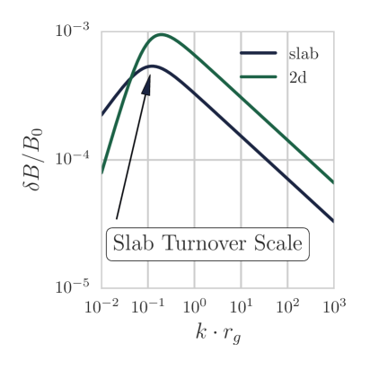
Figure 1: Example magnetic turbulence spectrum with $s_{\mathrm{slab}}=5/3$, $q_{\mathrm{slab}}=0$, $s_{\mathrm{2d}}=5/3$, $q_{\mathrm{2d}}=3/2$, $r_{\mathrm{slab}}=0.2$. The continuous spectrum is approximated here by a sum over $2048$ discrete wave modes with equal logarithmic spacing so that $\Delta\ln k=\Delta k/k$ is constant.

2.3 Numerical Setup

In the results presented in 4 below we chose the following parameters (in simulation units where $r_{g}=2\pi$): wavenumbers are uniformly distributed in log-space ($\Delta\ln k=\Delta k/k$ is constant) between the minimum and maximum $k_{min}=10^{-4}$ and $k_{max}=10^{6}$ respectively. These values are chosen so as to allow resonant interaction at most values of $\mu$. The spectral indices are $s_{\text{slab}}=5/3$, $s_{\text{2d}}=5/3$, $q_{\text{slab}}=0$, $q_{\text{2d}}=3/2$ (Shalchi & Weinhorst, 2009), and turbulence turnover scales $\ell_{\text{slab}}=\ell_{\text{2d}}=1$. This assumption is based on coupling between the ion gyroscale and turbulence length scale from collisionless Landau damping, which results in turbulence with turnover scale $\approx r_{g}$ (Schekochihin et al., 2009). Particles are initially uniformly distributed in $\mu$-space ensuring they interact with different parts of the spectrum. Their initial velocity is chosen to be $v=0.1c$ (see discussion in 5). The number of waves and particles per seed is $n_{w}=4096$ and $n_{p}=256$ respectively. The number of random seeds corresponding to distinct turbulence realisations for ensemble average $n_{s}=8$, which was found to be enough to achieve convergence. The total run time is set individually for each set of turbulence level, by using a small initial run to determine the approximate value of the diffusion time $t_{s}$ (see 3 and appendix A below) and then running the full simulation with $t_{\mathrm{max}}\gtrsim 100t_{s}$ in order to be able to capture the diffusion in each case. The integrator used is bulirsch-stoer from odeint (Ahnert & Mulansky, 2011) with relative and absolute tolerance $\varepsilon_{\text{rel}}=\varepsilon_{\text{abs}}=10^{-9}$. The particle trajectories are tracked and the scattering time $t_{s}$ and pitch-angle diffusion coefficient $D_{\mu\mu}$ are calculated. As this can be done in more than one way we explain our calculation method in 3 below.

3 Diffusion

In this section we motivate and explain our calculation of the pitch-angle diffusion coefficient $D_{\mu\mu}$. We briefly review the significance of this parameter and methods for measuring its value from simulation results. It is seen that the choice of $D_{\mu\mu}$ is also reliant on the choice of $\Delta t$, the time over which diffusion steps are measured. Note that $\Delta t$ provides a timescale for Monte–Carlo simulations which make use of diffusion models discussed here, and is distinct from the integration timestep of the simulation used in this work (see 2). We discuss choices of $\Delta t$ as they apply to numerical simulations and as they relate to the QLT and Bohm approximations.

3.1 Definition of $D_{\mu\mu}$

The particle population in a CR accelerator system can be encapsulated in the multi-particle phase space distribution function $f\left(x^{i},p^{i},t\right)$ where $\int_{\Omega}f\,\mathrm{d^{3}x}\mathrm{d^{3}p}$ is the number of particles in the phase-space volume $\Omega$, and $x^{i}$ and $p^{i}$ are respectively spatial coordinates and momentum coordinates. Its evolution is described by the Fokker-Planck equation (Hall, 1967; Schlickeiser, 2002),

$$\partial_{t}f+v^{i}\partial_{x^{i}}f+p^{-2}\partial_{p^{i}}\left(p^{2}D^{p_{i}p_{j}}\partial_{p^{j}}f\right)=0$$ (9)

where $p$ is momentum and $D$ is the diffusion tensor. For a derivation and background on this equation see Hall (1967); Newman (1973); Urch (1977); Schlickeiser (2002). We use the convenient momentum-space basis $\left(p_{r},p_{\phi},p_{\mu}\right)$ of radial, gyrophase and pitch-angle cosine respectively. We assume axisymmetry around $\boldsymbol{B}_{0}$, that scatterings are elastic, and ignore perpendicular and gyrophase motion. This gives symmetry in $x$, $y$, and $p_{\phi}$ and that $p_{r}=\left|p\right|$ is constant, hence our remaining dependent variables are just $z$ and $\mu$ this equation can be written as

$$\partial_{t}f+v\mu\partial_{z}f+\partial_{\mu}\left({D_{\mu\mu}}\partial_{\mu}f\right)=0$$ (10)

where by abuse of notation we have defined $D_{\mu\mu}$ as the component of the tensor $D$ in the direction of $\mu$, i.e. $D^{p^{\mu}p^{\mu}}=D_{\mu\mu}$ and assumed all other components are zero.

The parameter $D_{\mu\mu}$ typically depends on the pitch angle as well as the turbulence details and determines the particle trajectory by encapsulating the details of the turbulent wave-particle interaction (we neglect particle-particle interation). The problem of defining and measuring the diffusion coefficient $D_{\mu\mu}$ has been discussed at length in the literature, both in terms of the appropriate timescale over which to measure (Giacalone & Jokipii, 1999; Shalchi, 2006; Spanier & Wisniewski, 2011) and the appropriate way to calculate it (Knight & Klages, 2011; Shalchi, 2011). The difficulty arises from the fact that, unlike the classical hard-sphere scattering case, the diffusion does not occur in response to discrete events but rather a gradual collective interaction with the whole spectrum of magnetic turbulence simultaneously.

While there are several possible prescriptions for calculating $D_{\mu\mu}$, for the purposes of this work the mean square deviation (MSD) form (Jokipii, 1966; Blandford & Eichler, 1987; Tautz et al., 2013) is used,

$$D_{\mu\mu,\text{MSD}}\equiv\left<\frac{\left(\Delta\mu\right)^{2}}{\Delta t}\right>$$ (11)

where $\Delta\mu=\mu\left(t\right)-\mu\left(0\right)$ and the chevrons indicate an average over ensemble. This form is suitable because it allows the parameter $\Delta t$ to be tuned, and as we will discuss in 3.2 this determines what timescales can be resolved.

The MSD form is the most straightforward way of calculating $D_{\mu\mu}$. We note, however, that other methods exist. Of particular interest are the Taylor-Green-Kubo (TGK) integral and derivative methods. The TGK integral form (Tautz et al., 2013), $D_{\mu\mu,\text{TGKI}}\equiv\int_{0}^{\infty}\mathrm{d}t\left\langle\dot{\mu}\left(t\right)\dot{\mu}\left(0\right)\right\rangle$ where overdot indicates time derivative, is more amenable than MSD to analytic work. However this quantity is unsuitable for numerical work as the integral does not converge when the upper limit is taken to infinity. In numerical approximations, when the upper integration limit is taken to be $\Delta t$, it is identical to the MSD form (Shalchi, 2011). A third method, the TGK derivative form (Tautz et al., 2013) $D_{\mu\mu,\text{TGKD}}\equiv\frac{\mathrm{d}}{\mathrm{d}t}\left\langle\left(\Delta\mu\right)^{2}\right\rangle$, is the limit of $D_{\mu\mu,\text{MSD}}$ as $\Delta t\rightarrow 0$, however this form cannot be used since for $\Delta t$ too short only ballistic motion will be seen (Zank, 2014).

3.2 On the Proper Choice of the Diffusion Timestep $\Delta t$

As we show below in 4, the value of $D_{\mu\mu,\mathrm{MSD}}$ in (LABEL:msd1) is highly sensitive to the choice of $\Delta t$, the time over which $\Delta\mu$ is measured. In order to obtain a physically meaningful value for $D_{\mu\mu}$ the following must be considered. In the limit $\Delta t\rightarrow 0$ the diffusion coefficient approaches zero, regardless of the details of the diffusion, because the numerator in (LABEL:msd1) is second order in $\Delta t$, while the denominator is only first-order. On the other hand the value of $\Delta t$ cannot be too long. Since $\Delta\mu$ can be at most $2$ an arbitrarily large value of $\Delta t$ causes $D_{{\mu\mu}}$ to vanish.

Two useful timescales which will be employed are the scattering time $t_{s}$ and the diffusion time $t_{D}$. The scattering time $t_{s}$ can be defined as the expected time for the particle’s pitch angle to change by a $\Delta\vartheta$, typically $90\textdegree$, or equivalently, as in this paper, as the decorrelation time

$$t_{s}=\left\langle\int_{0}^{\infty}C_{\mu}\left(t,\tau\right)\mathrm{d}t\right\rangle_{\tau}$$ (12)

(Casse et al., 2002), where $C_{\mu}\left(t,\tau\right)=\left\langle\mu\left(t+\tau\right)\mu\left(t\right)\right\rangle/\left\langle\mu\left(t\right)^{2}\right\rangle$ is the autocorrelation of $\mu$ at time $t$ and $\left\langle\cdot\right\rangle_{t}$ indicates a time average. See appendix A for further details. We similarly define the diffusion time $t_{D}=1/\left\langle D_{\mu\mu}\right\rangle$, i.e. the time taken for the particle to significantly change pitch-angle so that $\Delta\mu\approx 1$.

The assumption that particles interact only resonantly with waves (as is assumed in QLT) requires that differences in $\mu$ are measured over many gyrotimes, so that the force contributions from nonresonant waves average to zero. In the weak turbulence regime QLT is known to be a good approximation (Shalchi, 2009b), and so we retain this constraint in order to recover QLT in this limit.

The Bohm approximation, on the other hand, assumes that the scattering time is roughly equal to the gyrotime, so that $\Delta t$ may not be much less than $t_{g}$. However as long as $\Delta\mu\ll 1$ values of $\Delta t>t_{g}$ may be used.

Neither the Bohm nor QLT type models include a description of frequent scattering, i.e. more than once per gyrotime. Since the particle may scatter to a significantly different pitch angle within a single gyrotime it can have a different resonant wavelength and hence interact with a different portion of the turbulence spectrum. Moreover at this point the particle is no longer undergoing gyromotion, and cannot be treated as a “scattering gyrocentre”. We can estimate the turbulence strength at which the scattering becomes more frequent than the gyration by equating the gyrotime $t_{g}$ with the diffusion time $t_{D}$. In order to have at least one scattering per diffusive timestep in this case we then must have $t_{g}\leq\Delta t$. However it is found that for strong turbulence, the scattering time is on the order of, or shorter than the gyrotime.

To conclude, any timestep must satisfy several upper and lower limits. Compatibility with the assumptions of QLT requires that $t_{g}\ll\Delta t\ll t_{D}$, and Bohm requires $t_{g}\lesssim\Delta t\ll t_{D}$. This imples that in order to use a diffusion model we must have $t_{g}<t_{D}$. We discuss below the conditions under which this requirement is met.

3.3 Anomalous Diffusion

Classical diffusion processes resulting from discrete scattering events in unbounded regions (e.g. gas diffusion) exhibit displacements of the form $\left\langle\left(\Delta x\right)^{2}\right\rangle\propto\Delta t$ for all timesteps $\Delta t$ much greater than the scattering time, and so $D_{xx}=\frac{\left\langle\left(\Delta x\right)^{2}\right\rangle}{\Delta t}$ is independent of $\Delta t$. This is also the case for the Bohm and QLT models. However, when turbulence is so strong that within each timestep $\mu$ changes significantly, this behaviour is not observed and the time dependence of the MSD is nonlinear (Metzler & Klafter, 2000). Hence we consider generalised diffusion models where

$$\left\langle\left(\Delta\mu\right)^{2}\right\rangle \propto\Delta t^{b}$$ (13)

with $b\neq 1$. This is known as anomalous diffusion (see e.g. Pommois et al. (2007); Shalchi & Weinhorst (2009); Bykov et al. (2017)). The physical mechanisms by which $D_{{\mu\mu}}$ can depend nonlinearly on $\Delta t$ are: directly though time-dependent turbulence, and indirectly through dependence on $\mu$. Solving (LABEL:anomalous_b) for $b$ gives $b=\frac{\mathrm{d}\ln D_{\mu\mu}}{\mathrm{d}\ln\Delta t}+1$ and this is used to identify the diffusion regime, as in Figures 2 and 3. The turbulence is time-independent since wave propagation and feedback are not included so any anomalous diffusion must be inherent to the scattering process. When the diffusion is not anomalous the choice of $\Delta t$ is seen to be arbitrary (within the constraints of 3.2) and in practice is chosen to be $20t_{g}$. Notably in the case of bounded diffusion like that of $\mu$, there is always a non-physical $b=-1$ regime for sufficiently large $\Delta t$.

4 Results

In this section we show the results of our simulations or particle transport. From the gathered data we calculate $D_{\mu\mu}$, and its time-dependence. We separately calculate the scattering time $t_{s}$ and finally use this data to find the Bohm exponent $\alpha$ and give its dependence on the turbulence strength.

4.1 Choice of $\Delta t$

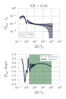
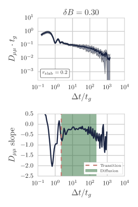
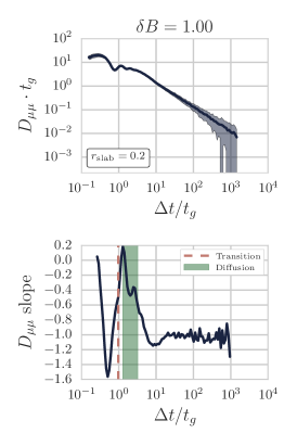
Figure 2: The upper plots show $D_{{\mu\mu}}$ (pitch-angle averaged) as a function of $\Delta t$ for $r_{\mathrm{slab}}=0.2$, with the solid line for the particle average and the shaded area representing one standard deviation. The lower plots show the average slope of $D_{{\mu\mu}}$ as a function of $\Delta t$, highlighting the transition from ballistic to subdiffusive behaviour ($\frac{\mathrm{d}\ln D_{\mu\mu}}{\mathrm{d}\ln\Delta t}<0$, dashed red line), and the diffusive regime ($\frac{\mathrm{d}\ln D_{\mu\mu}}{\mathrm{d}\ln\Delta t}\approx 0$, green shading). Notice that the diffusive range shrinks as the turbulence strength increases. These plots are in simulation units where $B_{0}=1$.

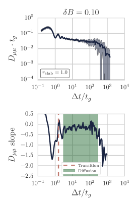
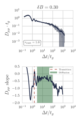
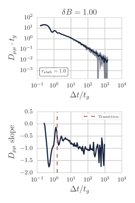
Figure 3: Same as time-test, but for $r_{\mathrm{slab}}=1$ (pure slab turbulence). The $\delta B/B_{0}=1$ case has no significant time region in which behaviour is diffusive since $t_{D}<t_{g}$ and the middle term of (LABEL:dmmucases) vanishes.

In time-test,time-test-sr1.0 (upper panels) we plot $D_{{\mu\mu}}$ against $\Delta t$ for various turbulence levels. The upper panels show $D_{\mu\mu}$ as a function of $\Delta t$. The main features are the initial ballistic phase, the diffusive phase ($b\approx 1$), and the subdiffusive ($b<1$) tail. As the turbulence level is increased the diffusive region shrinks and eventually disappears entirely. time-test,time-test-sr1.0 (lower panels) plot the slope $\frac{\mathrm{d}\ln D_{\mu\mu}}{\mathrm{d}\ln\Delta t}$ and allow us to clearly delineate the end of the ballistic phase (red dashed line) and the diffusive phase (green shading). This shows that in the weak turbulence case ($\delta B/B_{0}=0.1$) the behaviour after several gyrotimes become approximately diffusive over a wide range of $\Delta t$, as predicted by QLT.

We find that $D_{\mu\mu}$ initially increases quadratically while $\Delta t$ is short enough that the particle motion is ballistic (Tautz & Shalchi, 2011; Tautz et al., 2013). It then peaks, may remain constant for some range of of $\Delta t$ (depending on turbulence level), and then diminishes linearly due to the boundedness of $\mu$. Hence the diffusion coefficient is approximately described by

$$D_{\mu\mu}\left(\Delta t\right)\propto\begin{cases}\Delta t^{2}&\Delta t<t_{g}\\ \Delta t^{0}&t_{g}<\Delta t<t_{D}\\ \Delta t^{-1}&\Delta t>t_{D}\end{cases}$$ (14)

corresponding to the cases of anomalous diffusion index $b=$$3$, $1$, and $0$ respectively. There is also a sinusoidal component due to the gyromotion of the particle, which causes the observed turbulent magnetic field to rotate at the angular gyrofrequency $\omega_{g}=2\pi/t_{g}$.

The difference in $r_{\text{slab}}$ and hence lower two-dimensional turbulence strength in time-test-sr1.0 has the effect of enhancing the diffusion by a factor of order unity..

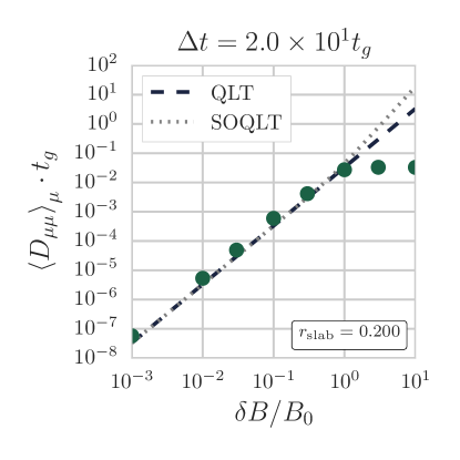
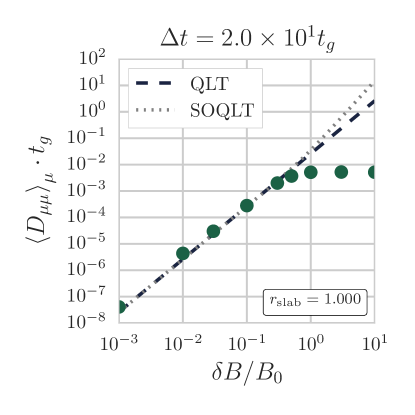
Figure 4: $D_{\mu\mu}$ (pitch-angle averaged) measured at $\Delta t=20t_{g}$ for various (slab-only) turbulence levels. Good agreement with the (SO)QLT models for weak turbulence. For turbulence levels $\delta B\gtrsim 1$ the measurement time $\Delta t$ of $20t_{g}$ is no longer within the diffusion regime (see time-test) and so the values are no longer meaningful.

In -measured-at20tg we show the diffusion coefficient as a function of turbulence level. It initially increases as $\delta B^{2}$ (QLT regime), gradually flattens around $\delta B/B_{0}=10^{-1}$ and stays roughly constant thereafter. We argue that this flattening is not physical but an artifact of the fact the we are measuring a bounded quantity $\Delta\mu$ over a time period longer than its dynamical time $1/D_{\mu\mu}$. Indeed, from time-test it can be seen that only for low-turbulence cases is there a region where

$$\frac{\mathrm{d}D_{\mu\mu}}{d\Delta t}\approx 0$$ (15)

(or equivalently that $b=1$) and the behaviour can be considered classically diffusive (i.e. independent of $\Delta t$). Once this region vanishes (see time-test) the process can no longer be treated as non-anomalous diffusion (c.f. Qin & Shalchi (2009)).

4.2 Validity of Bohm Approximation

One can model the diffusion of charged particles as a power law relationship between mean free path $\lambda_{\mathrm{mfp}}$ and gyroradius (Pommois et al., 2007). Here $\lambda_{\mathrm{mfp}}$ refers to the expected value of the distance travelled by a particle in the time it takes for $\vartheta$ to change by $\pi/2$; this corresponds to the mean free path between scatterings in the case of only right-angle collisions (Ellison et al., 1990; Summerlin & Baring, 2011),

$$\lambda_{\mathrm{mfp}}=\eta r_{g}^{\alpha}$$ (16)

where $\eta$ is the Bohm coupling constant and $r_{g}$ is suitably normalised. In particular the physical role of $\eta$ is to represent the effectiveness of the magnetic turbulence in diffusing the particles (see also 5.1). We refer to these as Bohm-type models. It is intentionally not specified whether the gyration radius $r_{g}$ refers to the radius of the gyration caused by the background field $B_{0}$, the total effective field $B_{\mathrm{eff}}=\sqrt{B_{0}^{2}+\delta B^{2}}$ or an intermediate approximation, as different authors make different choices here (see Vladimirov et al. (2006)). In this work the “effective” field gyroradius and gyrotime are denoted $r_{g}^{\prime}$ and $t_{g}^{\prime}$ respectively, as in Scattering-time-as.

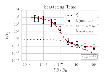
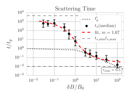
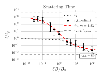
Figure 5: Scattering time $t_{s}$ as a function of turbulence level $\delta B/B_{0}$ with $r_{slab}=0.2$, $0.5$ and $1.0$. Here $t_{g}^{\prime}$ represents the “effective” gyrotime determined by the effective field $B_{\text{eff}}$. Points represent the ensemble and pitch-angle median of the measured scattering times for each turbulence level, and the error bars the first and third quartile . The red line is a fit with (LABEL:fitted_model), with the parameters indicated on the respective graph and in Best-fit-parameters.

In this work we take the “Bohm approximation” to mean $\alpha\approx 1$. This can be formulated equivalently as

$$t_{s}\approx t_{g}$$ (17)

(as long as $\eta$ is of order unity) meaning scattering occurs once per gyrotime. We present the ratio of the scattering time to gyrotime in Scattering-time-as. From the figure we see that this form of Bohm approximation is valid only around $\delta B/B_{0}\approx 1$ for the unmodified gyrotime $t_{g}$. However we find that the modified form of the Bohm approximation, $t_{g}^{\prime}\approx t_{s}$, is valid until $\delta B/B_{0}\approx 10$ . This behaviour does not continue to higher turbulence levels, and the scattering time instead asymptotes. Running the simulation with a smaller $\left[k_{\mathrm{min}},k_{\mathrm{max}}\right]$ range confirms that this behaviour is due to the finite wavelength cutoff in the turbulence spectrum.

Heuristically we can fit this with a sigmoid function, in Scattering-time-as we take

$$\log_{10}t_{s}/t_{g}=t_{s,\mathrm{min}}+\frac{t_{s,\mathrm{max}}-t_{s,\mathrm{min}}}{2}\left(1+\frac{m}{\pi}\arctan(-m\log_{10}\left(\delta B/B_{0}\right)\right)$$ (18)

where parameters $t_{s,\mathrm{max}}$ and $t_{s,\mathrm{min}}$ are respectively the low and high turbulence limits of the scattering time, and $m$ (not to be confused with the particle mass) is a free parameter determining the slope of the transition region. The best fit parameters from our results are as given in Best-fit-parameters.

$r_{\mathrm{slab}}$		$t_{s,\mathrm{max}}/t_{g}$	$t_{s,\mathrm{min}}/t_{g}$	$m$
$0.2$		$2.228\times 10^{3}$	$4.178\times 10^{-2}$	$2.573$
$0.5$		$4.571\times 10^{3}$	$1.038\times 10^{-2}$	$1.668$
$1.0$		$4.898\times 10^{3}$	$5.546\times 10^{-3}$	$1.230$

Table 1: Best fit parameters for (LABEL:fitted_model) applied to the data in Scattering-time-as. Parameters $t_{s,\mathrm{max}}$ and $t_{s,\mathrm{min}}$ are respectively the low and high turbulence limits of the scattering time, and $m$ determines the slope of the transition region.

Since $\lambda_{\mathrm{mfp}}=\eta r_{g}^{\alpha}$, $r_{g}=\frac{\gamma mv}{eB}\left(1-\mu^{2}\right)^{1/2}$, and $t_{s}=\frac{\lambda_{\mathrm{mfp}}}{v}$, the following relation holds:

$$t_{s}\propto v^{\alpha-1}B^{-\alpha}.$$ (19)

It is clear from Scattering-time-as and (LABEL:tspropbalpha) that the value of $\alpha$ must vary significantly between turbulence regimes, since otherwise a single power law would be observed. Hence no model with constant $\alpha$ can cover the entire turbulence range. Vladimirov et al. (2009) implicitly recognises this when interpolating between different values of $\alpha$ for different particle energies.

From (LABEL:tspropbalpha) the Bohm exponent $\alpha$ can be expressed as

$$\alpha=-\frac{\mathrm{d}\ln t_{s}}{\mathrm{d}\ln B_{\mathrm{eff}}}.$$

Reformulating in order to isolate the dependence on $\delta B$,

$$\alpha =-\frac{\mathrm{d}\ln t_{s}}{\mathrm{d}\ln\delta B}\frac{\mathrm{d}\ln\delta B}{\mathrm{d}\ln B_{\mathrm{eff}}}$$

$$=-\frac{\mathrm{d}\ln t_{s}}{\mathrm{d}\ln\delta B}\frac{B_{\mathrm{eff}}^{2}}{{\delta B}^{2}}$$

$$=\tilde{\alpha}\left(1+\left(\frac{\delta B}{B_{0}}\right)^{-2}\right)$$

where $\tilde{\alpha}=-\frac{\mathrm{d}\ln t_{s}}{\mathrm{d}\ln\delta B}$ is the slope of the data presented in Scattering-time-as. The values of this “auxillary Bohm exponent” are calculated using a simple finite difference method and are plotted in alpha-bohm-expo. These show that $\alpha$ varies over the intermediate turbulence regime, and indeed that for $r_{\mathrm{slab}}=1$ and $\delta B/B_{0}\gtrsim 1$ we find $\tilde{\alpha}\approx 1$, in good agreement with the “Bohm approximation” that $\alpha=1$. Using these numerical results as model for diffusive motion, a Monte-Carlo simulation of particle acceleration can accurately account for the turbulent dependence of mean free path in the entire regime of turbulence strength using values of $\alpha$ presented here. In particular the region between $0$ and $\approx 10$, which as we have discussed is not covered by existing models, is covered.

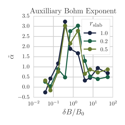
Figure 6: Auxillary Bohm exponent as a function of turbulence level for each of the considered values of $r_{slab}$ . This is calculated from the data in (5). It shows how a Bohm-type model can interpolate from weak up to intermediate and strong turbulence, by choosing the approximate values $\tilde{\alpha}=0$, $2.5$ and $0.7$ for these regions respectively.

We can estimate the value of the parameter $\eta$ in the regions where the slope of $t_{s}$ and $t_{g}^{\prime}$ are similar and hence $\eta\approx t_{s}/t_{g}^{\prime}$. For weak turbulence ($\delta B/B_{0}\ll 1$), $\alpha\approx 0$ and we find $\eta\approx 10^{3}$. For strong turbulence ($\delta B/B_{0}\gg 1$) we find $\eta\approx 1$. This is in agreement with the classical Bohm heuristic of scattering “once per gyrotime”.

5 Discussion

5.1 Diffusion Models

Bohm-type models supported by numerical evidence of 1-D Monte-Carlo simulations with power law Alfvén spectrum and observational evidence of ISEE-3 in the solar wind (Giacalone, J & Burgess, D & J. Schwartz, 1992), and more recently by PIC simulations when self-generated turbulence is included Caprioli & Spitkovsky (2014). It is not clear what the appropriate value of $\alpha$ is in each case, but some models are given in Spectral-Indices.

Model	$\alpha$
Constant/Low Energya	$0$
Kolmogorovb	$1/3$
Kraichnanb	$1/2$
Galacticc	$0.6\pm 0.1$
Bohmd	$1$
High-Energye	$2$

enumi Ellison et al. (1990) enumi Amato & Blasi (2005) enumi Shalchi (2009b) enumi Baring (2009); Summerlin & Baring (2011) enumi Toptygin & N. (1985)

Table 2: Values for the parameter $\alpha$ from various models, where all but the Galactic value are based on theory. Our model gives a value of $\alpha$ which varies with turbulence strength, but includes each of these at particular values of $\delta B/B_{0}.$

As discussed in Giacalone, J & Burgess, D & J. Schwartz (1992) a physical justification for the value of $\alpha$ is difficult due to the fact that “scattering events” are a simplification of the model and not an actual physical phenomenon. On the other hand Summerlin & Baring (2011) argue that $\alpha=1$ (the “Bohm limit”) is necessary for “physically meaningful diffusion” while claiming results are not strongly sensitive to this value. It can be shown (Shalchi, 2009a) that if the diffusion time is much shorter than the gyrotime then this assumption is equivalent to the claim that $D_{\mu\mu}\propto\frac{\delta B}{B_{0}}$, i.e. the diffusion is linearly dependent on the turbulence, as opposed to the quadratic dependence of QLT (Shalchi, 2015). Heuristically one can see this by noting that $\lambda_{\mathrm{mfp}}\propto D_{\mu\mu}^{-1}$ and $r_{g}\propto{\delta B}^{-1}$. In the limits of low and high energy particles where $r_{g}<1/k_{\mathrm{max}}$ or $r_{g}>1/k_{\mathrm{min}}$, there exists no wave with $k\approx 1/r_{g}$ and so resonant interaction is impossible and one obtains $\alpha=0$ and $\alpha=2$ respectively (Vladimirov et al., 2009).

Choosing a value of $\eta$, the Bohm coupling constant, is difficult, since it is not predicted by the model. It is a significant parameter, since it governs the anisotropy of the scattering (Giacalone & Jokipii, 1999) as well as the rate of energy gain in DSA (Dermer & Menon, 2009). It is suggested, for example, by Vladimirov et al. (2009), that $\eta$ may correspond to the magnetic correlation length for low energy ($\alpha=0$) particles. Comparison of Monte-Carlo and PIC results for laboratory plasmas found good agreement if a value of $\eta$ between $6$ and $25$ is used (Bultinck et al., 2010), while observations of Cas A suggest values between $2$ and $36$ (Stage et al., 2006). As shown in Scattering-time-as our results are consistent with $\eta\approx 1$ in the region of $\delta B/B_{0}\approx 3$, since here $t_{s}\approx t_{g}^{\prime}$.

Several other works have used numerical methods to find diffusion coefficients from simulated particle trajectories, e.g.Giacalone & Jokipii (1999); Shalchi (2009a); Reville et al. (2008); Tautz et al. (2013); Shalchi (2015). Giacalone & Jokipii (1999) examine weak and intermediate turbulence with isotropic and composite geometry (having equal correlation length in all directions). They find good agreement with QLT for diffusion parallel to $\boldsymbol{B}_{0}$, with an energy-independent difference of a factor of $10^{-2}$ from the QLT prediction for perpendicular diffusion. Pommois et al. (2007) vary the ratio of parallel and perpendicular magnetic correlation lengths $\frac{l_{\mathrm{cor}\parallel}}{l_{\mathrm{cor}\perp}}$ for fixed values of $\delta B/B_{0}$ weak and intermediate turbulence and find a variety of distinct transport regimes emerge as a function of Kubo number $K=\frac{\delta B}{B_{0}}\frac{l_{\mathrm{cor}\parallel}}{l_{\mathrm{cor}\perp}}$. In particular they find anomalous diffusion for slab and isotropic turbulence, but non-anomalous diffusion for $2d$ wave geometry. Shalchi (2015) provides a theoretical classification of some of these regimes in the limit of large or vanishing Kubo number. In our work the Kubo number is either $0$ (in the case of $r_{\text{$\mathrm{slab}$}}=1$) or equal to $\delta B/B_{0}$, since both correlation lengths are equal. In this context our results may explain why varying the Kubo number is observed by Pommois et al. (2007) to change the anomalous index associated with the diffusion.

It is also possible to choose other length scales in place of $r_{g}$ where other processes dominate, e.g. turbulence correlation length or vortex scale (Vladimirov, 2009).

5.2 Justifications for the Bohm Approximation

It is commonly accepted that Bohm diffusion is a heuristic, currently without a rigorous physical derivation (Krall & Trivelpiece, 1973; Casse et al., 2002), but it is nevertheless widely used in astrophysics under various justifications. There is analytic (Shalchi, 2009a) and numerical (Caprioli & Spitkovsky, 2014) evidence that it is a useful approximation for turbulence levels close to unity, this is in agreement with the results presented above. In Vladimirov, Ellison, & Bykov (2006) it is claimed that a more physically realistic treatment is necessary, but that a better model of mean free paths for strong turbulence is analytically intractable (see Bykov & Toptygin (1992)). They claim their results are not especially sensitive to the diffusion model and on that basis it is valid to use the simpler Bohm prescription. As we have argued however, the transport can vary greatly between different turbulence levels, and if a simulation is to track particles and waves across the many orders of magnitude in energy that are required for DSA then it must account for these differences.

In order to participate in DSA a particle must diffuse efficiently enough that the shock does not outrun it. For this it is necessary that the turbulence be strong, or that the diffusion be at least as strong as Bohm (Achterberg et al., 2001). This has tentative observational support in SN1006 (Allen et al., 2008). In the context of our results this would imply that the turbulence level in this environment is very close to unity.

5.3 Relevance to Astrophysical Environments

	SNR		GRBc		AGN a
	Max	Mean	Internal Shocks	Afterglowi	Flare
$B_{0}$	$100\mathrm{\mu G}$d	$5\mathrm{\mu G}$ ef	$10^{6}\mathrm{G}$	$1\mathrm{G}$	$10^{3}\mathrm{G}$
$\delta B/B$	$5$b	$1$b		$5$g
$E$	$100\mathrm{TeV}$e	$10\mathrm{MeV}$h	$100\mathrm{MeV}$	$100\mathrm{GeV}$	$100\mathrm{keV}$
$\gamma$	$10^{5}$ e	$1.01$h	$1.1$	$100$	$\gtrsim 1$
$t_{g}$	$10^{6}\mathrm{s}$	$10^{2}\mathrm{s}$	$10^{-10}\mathrm{s}$	$10^{-2}\mathrm{s}$	$10^{-6}\mathrm{s}$
$r_{g}$(at $\mu=1$)	$10^{14}\mathrm{m}$	$10^{5}\mathrm{m}$	$10^{-2}\mathrm{m}$	$10^{6}\mathrm{m}$	$1\mathrm{m}$

enumi Di Matteo (1998) enumi Bell (2004) enumi Piran (2005)(assuming equal proton and electron temperatures) enumi Caprioli et al. (2009) enumi Reynolds & Keohane (1999) enumi Woolsey et al. (2001) enumi Mizuno et al. (2011) enumi Guo et al. (2014) enumi (assuming upstream protons entering shock with $\gamma=100$)

Table 3: Approximate typical astrophysical parameters for supernova remnants (SNRs), gamma-ray bursts (GRBs) and active galactic nuclei (AGNs). Rows respectively correspond to: background magnetic field strength, magnetic turbulence ratio, average fluid-frame proton energy and Lorentz factor, gyrotime and gyroradius. Blank cells indicate data was unavailable.

Approximate-typical-astrophyisca gives estimates of the relevant parameters for protons in some candidate accelerator environments. The choice of $\Delta t$ ultimately determines what phenomena can be treated by modelling a system using (LABEL:mufokkerplanck), or equivalently the minimum timescale that can be resolved by any simulation using $D_{{\mu\mu}}$ as a parameter. There are several such timescales which may be relevant. Two natural choices are: the gyrotime of the particle $t_{g}$ and the wave crossing time $t_{w}=\frac{2\pi}{k_{max}}$, where $k_{\mathrm{max}}$ is the largest wavenumber in the spectrum. However $t_{g}$ is too short to average out nonresonant interactions, and Vladimirov et al. (2009) show that $k_{\mathrm{max}}$ may be as large as $10^{2}/r_{g}$ making $t_{w}$ even shorter.

The physical significance of the $\Delta t$ is manifest in microphysical processes which may play a role in particle acceleration. The growth time of relevant plasma instabilities such as Bell (Reville et al., 2008; Bai et al., 2014) and Weibel (Schlickeiser & Shukla, 2003) must be resolved by the diffusive timestep of a multi-physics simulation. This is because these are mechanisms by which anisotropies feed the magnetic turbulence and so are tightly coupled to diffusion.

Timescale			SNR	GRB Jeta	GRB Afterglow	AGNb
Gyration		$t_{g}=\frac{2\pi\gamma m}{eB_{0}}$	$10^{2}\mathrm{s}$	$10^{-10}\mathrm{s}$	$10^{-2}\mathrm{s}$	$10^{-6}\mathrm{s}$
Diffusion		$t_{D}=1/D_{\mu\mu}$	$10^{1}\mathrm{s}$		$10^{0}\mathrm{s}$
Scattering		$t_{s}=\int_{0}^{\infty}C(\tau)\mathrm{d}\tau$	$10^{3}\mathrm{s}$		$10^{1}\mathrm{s}$
Wave Crossing		$t_{w}=\frac{1}{\mu v}\frac{2\pi}{k_{\mathrm{max}}}$		$10^{-8}\mathrm{s}$	$10^{-4}\mathrm{s}$
Alfvén Crossing		$t_{A}=L_{\mathrm{system}}/v_{A}$		$10^{3}\mathrm{s}$	$10^{7}\mathrm{s}$	$10^{3}\mathrm{s}$

enumi Piran (2005) enumi Di Matteo (1998)

Table 4: Table of order-of-magnitude estimates of relevant time scales. Each of these provides a upper bound for a simulation timestep $\Delta t$. Diffusion times are estimates using the data from time-test, and scattering times from Scattering-time-as, both assuming $r_{\text{slab}}=0.2$. Blank cells indicate data was unavailable.

In the presented simulations we have restricted our attention to nonrelativistic particle velocities, which is justifiable at least for the majority of particles (see Approximate-typical-astrophyisca) but not for the high-energy cosmic-ray tail of the energy distribution. Furthermore since the Lorentz force law ((LABEL:lorentz-cov)) is manifestly covariant, the model considered in this work is applicable in principle to particles of relativistic energies, with the caveat that the resonance condition $k_{\text{max}}>1/r_{g}>k_{\text{min}}$ will not satisfied for particles of very large gyroradius. The limiting wavelength $2\pi/k_{\text{min}}$ may be as large as the system size $L$ but, depending on the turbulence generation mechanism, there may be very little magnetic energy available at this scale. Outside of the test-particle approximation, if a large share of the plasma’s energy is fed into the cosmic ray current, then the self-generated turbulence may increase in wavelength along with the typical gyroradius of the particles, and so maintain the resonance condition. Furthermore as $B$ becomes large the Alfvén speed $v_{A}$ approaches $c$ and the associated electric field $E$ becomes non-negligible. In this case particles will gain kinetic energy $T$ via the time component of (LABEL:lorentz-cov), $\partial_{t}T=ev\cdot E$. While this situation may well arise in acceleration environments, it significantly complicates the model and is deferred to future work.

6 Conclusions

In this paper we have shown that, while a comprehensive model of cosmic ray transport in accelerators is necessary for understanding the origins of high-energy cosmic rays, existing diffusion models are limited and may not cover some relevant ranges of parameters. This is because current analytic approaches (QLT, Bohm) rely on approximations which are invalid in important turbulence regimes.

The applicability of the diffusion model depends on the timestep/measuring time $\Delta t$, the choice of which depends on several factors. It is bounded below by the wave crossing time, the gyrotime, and also the relevant dynamical timescale for other relevant phenomena (e.g. plasma instabilities) and is bounded above by the diffusion time, as demonstrated in 4.1. For strong turbulence therefore, there may be no region in which a valid $\Delta t$ exists. In the absence of such a $\Delta t$ it is not meaningful to treat the problem as diffusive and more sophisticated models, e.g. anomalous diffusion, must be used. To this end we have measured the anomalous diffusion exponent $\tilde{\alpha}\left(\delta B\right)$ (alpha-bohm-expo).

We find that $\tilde{\alpha}\approx 0$ at low turbulence levels as expected from quasilinear theory. Its value then peaks at $\approx 3$ for intermediate $\delta B\approx B_{0}$ turbulence and then settles to $0.5<\tilde{\alpha}<1$.

The Bohm approximation, while generally applied for its convenience has been shown to be generally inapplicable to the case of diffusion in collisionless plasmas of the type described here. As we show, for environments with intermediate turbulence, the heuristic “Bohm-type” models of equation (1) do not accurately describe the observed dependence of scattering time on turbulence level. This is because they necassarily cannot capture the varying $\alpha$ seen in our simulation results, hence we propose that a more comprehensive model encapsulating the turbulence dependence is necessary, e.g. a model of the form:

$$\lambda_{\mathrm{mfp}}=\eta r_{g}^{\alpha\left(\delta B\right)}$$

Where the function $\alpha\left(\delta B\right)$ is determined beforehand in a numerical simulation which includes the details of the scattering microphysics, as we have done in this work. We have presented (LABEL:fitted_model) as a initial realisation of such a function.

In this work we do not treat feedback from particles to waves. However this effect can be significant when treating shock dynamics(Caprioli et al., 2009; Allen et al., 2008), in particular the acceleration process may dramatically change the shape of the wave spectrum (see e.g. Vladimirov et al. (2009)). This will be included in a future work.

Appendix A Calculation of Scattering Time

In order to calculate $t_{s}$ we use a method similar to that of Casse et al. (2002). While a classical particle undergoing a deterministic process has its past and future fully determined by its instantaneous position and velocity, a particle undergoing stochastic diffusion gradually “forgets” its past state. This loss of information can be quantified, for $\mu\left(t\right)$ real, using the so-called autocorrelation function,

$$C_{\mu}\left(t,\tau\right)=\frac{\left\langle\mu\left(t+\tau\right)\mu\left(t\right)\right\rangle}{\left\langle\mu\left(t\right)^{2}\right\rangle}$$ (A1)

where chevrons indicate any of three types of average: magnetic turbulence ensemble, chaotic motion ensemble, or temporal. If either of the former two types of chaos are ergodic, then they are equivalent to the temporal average, in which case (LABEL:cttau) simplifies to

$$C_{\mu}\left(\tau\right) =\frac{\left\langle\mu\left(t+\tau\right)\mu\left(t\right)\right\rangle_{t}}{\left\langle\mu\left(t\right)^{2}\right\rangle_{t}}$$

$$=\frac{\int_{-\infty}^{\infty}\mu\left(t+\tau\right)\mu\left(t\right)\,\mathrm{d}t}{\int_{-\infty}^{\infty}\mu\left(t\right)^{2}\,\mathrm{d}t}$$

$$=\frac{\mu\left(\tau\right)*\mu\left(-\tau\right)}{\left\|\mu\right\|^{2}}$$

where $*$ indicates convolution and $\left\|\cdot\right\|$ is the standard norm. If we now apply the convolution theorem and omit the $\tau$ for clarity,

$$\mathcal{F}C_{\mu} =\left(\mathcal{F}\mu\right)\left(\mathcal{F}\mu\right)^{\ast}/\left\|\mu\right\|^{2}$$

$$C_{\mu} =\mathcal{F}^{-1}\left|\mathcal{F}\mu\right|^{2}/\left\|\mu\right\|^{2}$$

where $\mathcal{F}$ is the Fourier transform, asterisk denotes complex conjugate, and $\left|\cdot\right|$ gives the magnitude of a complex number. This is known as Wiener-Khinchin form of the autocorrelation, and is the form used in this work for the purposes of numerical calculation since it is much more computationally efficient than the convolution form.

Formally the scattering time is then given by

$$t_{s}=\int_{0}^{\infty}C_{\mu}\left(\tau\right)\mathrm{d}\tau.$$

In the case of a classical Gaussian diffusion we expect the autocorrelation to decay exponentially, $C_{\mu}\left(\tau\right)=e^{-\alpha\tau}$ for some real parameter $\alpha$ and so we simply find $t_{s}=1/\alpha$. In the present work however, $C_{\mu}\left(\tau\right)$ is found to be highly oscillatory. Numerical integrals of this type are notoriously difficult to perform reliably, and for this reason we make the following simplifying assumption, that the numerical $C_{\mu}$s measured in this work are the product of various oscillating signals, and an exponentially decaying exponential envelope, so that $C_{\mu}\left(\tau\right)=\Re e^{t\left(\alpha+\beta i\right)}$, where $\beta$ is an ignorable real parameter, and $\Re$ takes the real part of a complex number. Here the decay constant $\alpha$ is the reciprocal of $t_{s}$ as above and this is the value that is presented in our results.

Care must be taken when using this method, as the finite length of the $C_{\mu}$ measurement means that even in the absence of diffusion $C_{\mu}$ will exhibit a $1/\tau$ envelope behaviour, with a slope of $-1/t_{\max}$, corresponding to a best fit scattering time of $t_{\mathrm{max}}\left(1-e^{-1}\right)$. To avoid measuring this spurious signal and have the real diffusion dominate, the $t_{\mathrm{max}}$ must be set to at least $2t_{s}$. Since $t_{s}$ cannot be known beforehand, this is achieved iteratively by increasing $t_{\mathrm{max}}$ until a good fit is obtained.

References

- Achterberg et al. (2001) Achterberg, A., Gallant, Y. A., Kirk, J. G., & Guthmann, A. W. 2001, Monthly Notices of the Royal Astronomical Society, 328, 393
- Ahnert & Mulansky (2011) Ahnert, K., & Mulansky, M. 2011, AIP Conference Proceedings, 1389, 1586
- Allen et al. (2008) Allen, G. E., Houck, J. C., & Sturner, S. J. 2008, The Astrophysical Journal, 683, 773
- Amato & Blasi (2005) Amato, E., & Blasi, P. 2005, 80, 11
- Bai et al. (2014) Bai, X.-N., Caprioli, D., Sironi, L., & Spitkovsky, A. 2014, arXiv:1412.1087
- Baring (2009) Baring, M. G. 2009, in AIP Conference Proceedings (AIP), 294–299
- Bell (1978) Bell, A. R. 1978, Monthly Notices of the Royal Astronomical Society, 182, 147
- Bell (2004) —. 2004, Monthly Notices of the Royal Astronomical Society, 353, 550
- Bell (2014) —. 2014, Brazilian Journal of Physics, 44, 415
- Bieber et al. (1996) Bieber, J. W., Wanner, W., & Matthaeus, W. H. 1996, Journal of Geophysical Research: Space Physics, 101, 2511
- Birdsall & Langdon (1985) Birdsall, C. K., & Langdon, A. B. 1985, Plasma physics via computer simulation (McGraw-Hill), 479
- Blandford & Eichler (1987) Blandford, R., & Eichler, D. 1987, Physics Reports, 154, 1
- Bohm (1949) Bohm, D. 1949, The characteristics of electrical discharges in magnetic fields,, 1st edn. (New York,: McGraw-Hill,)
- Bret & Pe’er (2018) Bret, A., & Pe’er, A. 2018, arXiv:1803.09744
- Bultinck et al. (2010) Bultinck, E., Mahieu, S., Depla, D., & Bogaerts, A. 2010, Journal of Physics D: Applied Physics, 43, 292001
- Bykov et al. (2017) Bykov, A. M., Ellison, D. C., & Osipov, S. M. 2017, Physical Review E, 95, arXiv:1703.01160
- Bykov et al. (2014) Bykov, A. M., Ellison, D. C., Osipov, S. M., & Vladimirov, A. E. 2014, The Astrophysical Journal, 789, 137
- Bykov & Toptygin (1992) Bykov, A. M., & Toptygin, I. N. 1992, Zhurnal Eksperimental’noi i Teoreticheskoi Fiziki (ISSN 0044-4510), 101, 866
- Caprioli et al. (2010a) Caprioli, D., Amato, E., & Blasi, P. 2010a, Astroparticle Physics, 33, 307
- Caprioli et al. (2009) Caprioli, D., Blasi, P., Amato, E., & Vietri, M. 2009, Monthly Notices of the Royal Astronomical Society, 395, 895
- Caprioli et al. (2010b) Caprioli, D., Kang, H., Vladimirov, A. E., & Jones, T. W. 2010b, Monthly Notices of the Royal Astronomical Society, 407, 1773
- Caprioli & Spitkovsky (2014) Caprioli, D., & Spitkovsky, A. 2014, The Astrophysical Journal, 794, 47
- Casse et al. (2002) Casse, F., Lemoine, M., & Pelletier, G. 2002, Physical Review D, 65, arXiv:0109223
- Dermer & Menon (2009) Dermer, C. D., & Menon, G. 2009, High Energy Radiation from Black Holes (Princeton: Princeton University Press), doi:10.1515/9781400831494
- Di Matteo (1998) Di Matteo, T. 1998, Monthly Notices of the Royal Astronomical Society, 299, L15
- Ellison et al. (1990) Ellison, D., Reynolds, S., & Jones, F. 1990, The Astrophysical Journal
- Ellison & Double (2002) Ellison, D. C., & Double, G. P. 2002, Astroparticle Physics, 18, 213
- Ellison et al. (2013) Ellison, D. C., Warren, D. C., & Bykov, A. M. 2013, The Astrophysical Journal, 776, 46
- Fermi (1949) Fermi, E. 1949, Physical Review, 75, 1169
- Ferrand et al. (2014) Ferrand, G., Danos, R. J., Shalchi, A., et al. 2014, The Astrophysical Journal, 792, 133
- Frederiksen et al. (2004) Frederiksen, J. T., Hededal, C. B., Haugbølle, T., & Nordlund, Å. 2004, The Astrophysical Journal, 608, L13
- Giacalone & Jokipii (1999) Giacalone, J., & Jokipii, J. 1999, The Astrophysical Journal, 20, 204
- Giacalone, J & Burgess, D & J. Schwartz (1992) Giacalone, J & Burgess, D & J. Schwartz, S. 1992, ESA, Study of the Solar-Terrestrial System, 65
- Gray et al. (1996) Gray, P. C., Pontius, D. H., & Matthaeus, W. H. 1996, Geophysical Research Letters, 23, 965
- Guo et al. (2014) Guo, X., Sironi, L., & Narayan, R. 2014, The Astrophysical Journal, 794, 153
- Hall (1967) Hall, D. E. 1967, Physics of Fluids, 10, 2620
- Hussein & Shalchi (2014) Hussein, M., & Shalchi, A. 2014, Astrophysical Journal, 785, 31
- Hussein et al. (2015) Hussein, M., Tautz, R. C., & Shalchi, A. 2015, Journal of Geophysical Research: Space Physics, 120, 4095
- Jokipii (1966) Jokipii, J. R. 1966, The Astrophysical Journal, 146, 480
- Jokipii (1972) —. 1972, 9
- Kirk & Heavens (1989) Kirk, J. G., & Heavens, A. F. 1989, Monthly Notices of the Royal Astronomical Society, 239, 995
- Knight & Klages (2011) Knight, G., & Klages, R. 2011, Physical Review E - Statistical, Nonlinear, and Soft Matter Physics, 84, arXiv:1107.5293
- Krall & Trivelpiece (1973) Krall, N. A., & Trivelpiece, A. W. 1973, Principles of Plasma Physics. Krall
- Lagage & Cesarsky (1983) Lagage, P. O., & Cesarsky, C. J. 1983, Astronomy and Astrophysics, 125, 249
- Li et al. (1997) Li, Y., Yoon, P. H., Wu, C. S., et al. 1997, Physics of Plasmas, 4, 4103
- Lucek & Bell (2000) Lucek, S. G., & Bell, A. R. 2000, Mon. Not. R. Astron. Soc, 314, 65
- Mace et al. (2000) Mace, R. L., Matthaeus, W. H., & Bieber, J. W. 2000, The Astrophysical Journal, 538, 192
- Malkov (1997) Malkov, M. A. 1997, The Astrophysical Journal, 485, 638
- Masters et al. (2017) Masters, A., Sulaiman, A. H., Stawarz, Ł., et al. 2017, The Astrophysical Journal, 843, 147
- Metzler & Klafter (2000) Metzler, R., & Klafter, J. 2000, Physics Reports, 339, 1
- Mizuno et al. (2011) Mizuno, Y., Pohl, M., Niemiec, J., et al. 2011, Astrophysical Journal, 726, arXiv:1011.2171
- Newman (1973) Newman, C. E. 1973, Journal of Mathematical Physics, 14, 502
- Pelletier (2001) Pelletier, G. 2001, Physics and Astrophysics of Ultra High Energy Cosmic Rays, 576, 58
- Piran (2005) Piran, T. 2005, in AIP Conference Proceedings, Vol. 784, 164–174
- Pommois et al. (2007) Pommois, P., Zimbardo, G., & Veltri, P. 2007, Physics of Plasmas, 14, 012311
- Qin & Shalchi (2009) Qin, G., & Shalchi, a. 2009, The Astrophysical Journal, 707, 61
- Reville et al. (2008) Reville, B., O’Sullivan, S., Duffy, P., & Kirk, J. G. 2008, Monthly Notices of the Royal Astronomical Society, 386, 509
- Reynolds & Keohane (1999) Reynolds, S. P., & Keohane, J. W. 1999, The Astrophysical Journal, 525, 368
- Schekochihin et al. (2009) Schekochihin, a. a., Cowley, S. C., Dorland, W., et al. 2009, Astrophysical Journal, Supplement Series, 182, 310
- Schlickeiser (2002) Schlickeiser, R. 2002, Cosmic Ray Astrophysics (Springer Berlin Heidelberg), doi:10.1007/978-3-662-04814-6
- Schlickeiser & Shukla (2003) Schlickeiser, R., & Shukla, P. K. 2003, The Astrophysical Journal, 599, L57
- Shalchi (2005) Shalchi, A. 2005, Physics of Plasmas, 12, 1
- Shalchi (2006) —. 2006, Astronomy and Astrophysics, 448, 809
- Shalchi (2009a) —. 2009a, Astroparticle Physics, 31, 237
- Shalchi (2009b) —. 2009b, Nonlinear Cosmic Ray Diffusion Theories (Springer Berlin Heidelberg), doi:10.1007/978-3-642-00309-7
- Shalchi (2011) —. 2011, Physical Review E, 83, 046402
- Shalchi (2015) —. 2015, Physics of Plasmas, 22, 010704
- Shalchi et al. (2008) Shalchi, A., Bieber, J. W., & Matthaeus, W. H. 2008, A&A, 381, 371
- Shalchi & Weinhorst (2009) Shalchi, A., & Weinhorst, B. 2009, Advances in Space Research, 43, 1429
- Silva et al. (2003) Silva, L. O., Fonseca, R. a., Tonge, J., et al. 2003, 3, 121
- Sironi & Spitkovsky (2011) Sironi, L., & Spitkovsky, A. 2011, The Astrophysical Journal, 726, 75
- Spanier & Wisniewski (2011) Spanier, F., & Wisniewski, M. 2011, Astrophysics and Space Sciences Transactions, 7, 21
- Spitkovsky (2008) Spitkovsky, A. 2008, The Astrophysical Journal, 682, L5
- Stage et al. (2006) Stage, M. D., Allen, G. E., Houck, J. C., & Davis, J. E. 2006, Nature Physics, 2, 18
- Summerlin & Baring (2011) Summerlin, E. J., & Baring, M. G. 2011, The Astrophysical Journal, 745, 63
- Tautz (2010) Tautz, R. C. 2010, Computer Physics Communications, 181, 71
- Tautz et al. (2013) Tautz, R. C., Dosch, A., Effenberger, F., Fichtner, H., & Kopp, A. 2013, Astronomy & Astrophysics, 558, A147
- Tautz & Shalchi (2010) Tautz, R. C., & Shalchi, A. 2010, Physics of Plasmas, 17, doi:10.1063/1.3530185
- Tautz & Shalchi (2011) —. 2011, Astrophysical Journal, 735, doi:10.1088/0004-637X/735/2/92
- Toptygin & N. (1985) Toptygin, I. N., & N., I. 1985, Cosmic rays in interplanetary magnetic fields, 118
- Tu & Marsch (1995) Tu, C. Y., & Marsch, E. 1995, Space Science Reviews, 73, 1
- Urch (1977) Urch, I. H. 1977, Astrophysics and Space Science, 46, 389
- Vladimirov (2009) Vladimirov, A. 2009, PhD thesis, NCSU
- Vladimirov et al. (2006) Vladimirov, A., Ellison, D. C., & Bykov, A. 2006, 1246
- Vladimirov et al. (2008) Vladimirov, A. E., Bykov, A. M., & Ellison, D. C. 2008, 20
- Vladimirov et al. (2009) —. 2009, The Astrophysical Journal, 703, L29
- Voelk & Biermann (1988) Voelk, H. J., & Biermann, P. L. 1988, The Astrophysical Journal, 333, L65
- Woolsey et al. (2001) Woolsey, N. C., Ali, Y. A., Evans, R. G., et al. 2001, Physics of Plasmas, 8, 2439
- Zank (2014) Zank, G. P. 2014, Lecture Notes in Physics, Vol. 877, Transport Processes in Space Physics and Astrophysics (New York, NY: Springer New York), 77–136, doi:10.1007/978-1-4614-8480-6