On Learning Markov Chains

Abstract

The problem of estimating an unknown discrete distribution from its samples is a fundamental tenet of statistical learning. Over the past decade, it attracted significant research effort and has been solved for a variety of divergence measures. Surprisingly, an equally important problem, estimating an unknown Markov chain from its samples, is still far from understood. We consider two problems related to the min-max risk (expected loss) of estimating an unknown $k$-state Markov chain from its $n$ sequential samples: predicting the conditional distribution of the next sample with respect to the KL-divergence, and estimating the transition matrix with respect to a natural loss induced by KL or a more general $f$-divergence measure.

For the first measure, we determine the min-max prediction risk to within a linear factor in the alphabet size, showing it is $\Omega(k\log\log n/n)$ and $\mathcal{O}(k^{2}\log\log n/n)$. For the second, if the transition probabilities can be arbitrarily small, then only trivial uniform risk upper bounds can be derived. We therefore consider transition probabilities that are bounded away from zero, and resolve the problem for essentially all sufficiently smooth $f$-divergences, including KL-, $L_{2}$-, Chi-squared, Hellinger, and Alpha-divergences.

1 Introduction

Many natural phenomena are inherently probabilistic. With past observations at hand, probabilistic models can therefore help us predict, estimate, and understand, future outcomes and trends. The two most fundamental probabilistic models for sequential data are i.i.d. processes and Markov chains. In an i.i.d. process, for each $i\geq{1}$, a sample $X_{i}$ is generated independently according to the same underlying distribution. In Markov chains, for each $i\geq 2$, the distribution of sample $X_{i}$ is determined by just the value of $X_{i-1}$.

Let us confine our discussion to random processes over finite alphabets, without loss of generality, assumed to be $[k]:=\{1,2,\ldots,k\}$. An i.i.d. process is defined by a single distribution $p$ over $[k]$, while a Markov chain is characterized by a transition probability matrix $M$ over $[k]\times[k]$. We denote the initial and stationary distributions of a Markov model by $\mu$ and $\pi$, respectively. For notational consistency let $P=(p)$ denote an i.i.d. model and $P=(M)$ denote a Markov model.

Having observed a sample sequence $X^{n}:=X_{1},\ldots,X_{n}$ from an unknown i.i.d. process or Markov chain, a natural problem is to predict the next sample point $X_{n+1}$. Since $X_{n+1}$ is a random variable, this task is typically interpreted as estimating the conditional probability distribution $P_{x^{n}}:=\text{Pr}{(X_{n+1}=\cdot|X^{n}=x^{n})}$ of the next sample point ${X_{n+1}}$.

Let $[k]^{*}$ denote the collection of all finite-length sequences over $[k]$.

Therefore, conditioning on $X^{n}=x^{n}$, our first objective is to estimate the conditional distribution To be more precise, we would like to find an estimator $\hat{P}$, that associates with every sequence $x^{n}\in[k]^{*}$ a distribution $\hat{P}_{x^{n}}$ over $[k]$ that approximates $P_{x^{n}}$ in a suitable sense.

Perhaps a more classical problem is parameter estimation, which describes the underlying process. An i.i.d. process is completely characterized by $P_{x^{n}}=p$, hence this problem coincides with the previous one. For Markov chains, we seek to estimate the transition matrix $M$. Therefore, instead of producing a probability distribution $\hat{P}_{x^{n}}$, the estimator $\hat{M}$ maps every sequence $x^{n}\in[k]^{*}$ to a transition matrix $\hat{M}_{x^{n}}$ over $[k]\times[k]$.

For two distributions $p$ and $q$ over $[k]$, let $L(p,q)$ be the loss when $p$ is approximated by $q$. For the prediction problem, we measure the performance of an estimator $\hat{P}$ in terms of its prediction risk,

$$\rho_{n}^{L}(P,\hat{P}):=\operatorname*{\mathds{E}}_{X^{n}\sim P}[L(P_{X^{n}},\hat{P}_{X^{n}})]=\sum_{x^{n}\in[k]^{n}}P(x^{n})L(P_{x^{n}},\hat{P}_{x^{n}}),$$

the expected loss with respect to the sample sequence $X^{n}$, where $P(x^{n}):=\text{Pr}{(X^{n}=x^{n})}$.

For the estimation problem, we quantify the performance of the estimator by estimation risk. We first consider the expected loss of $\hat{M}$ with respect to a single state $i\in[k]$:

$$\operatorname*{\mathds{E}}_{X^{n}\sim(M)}[L(M(i,\cdot),\hat{M}_{X^{n}}(i,\cdot))].$$

We then define the estimation risk of $\hat{M}$ given sample sequence $X^{n}$ as the maximum expected loss over all states,

$${\varepsilon}_{n}^{L}(M,\hat{M}):=\max_{i\in[k]}\operatorname*{\mathds{E}}_{X^{n}\sim(M)}[L(M(i,\cdot),\hat{M}_{X^{n}}(i,\cdot))].$$

While the process $P$ we are trying to learn is unknown, it often belongs to a known collection $\mathscr{P}$. The worst prediction risk of an estimator $\hat{P}$ over all distributions in $\mathscr{P}$ is

$$\rho_{n}^{L}(\mathscr{P},\hat{P}):=\max_{P\in\mathscr{P}}\rho_{n}^{L}(P,\hat{P}).$$

The minimal possible worst-case prediction risk, or simply the minimax prediction risk, incurred by any estimator is

$$\rho_{n}^{L}(\mathscr{P}):=\min_{\hat{P}}\rho_{n}^{L}(\mathscr{P},\hat{P})=\min_{\hat{P}}\max_{P\in\mathscr{P}}\rho_{n}^{L}(P,\hat{P}).$$

The worst-case estimation risk ${\varepsilon}_{n}^{L}(\mathscr{P},\hat{M})$ and the minimax estimation risk ${\varepsilon}_{n}^{L}(\mathscr{P})$ are defined similarly. Given $\mathscr{P}$, our goals are to approximate the minimax prediction/estimation risk to a universal constant-factor, and to devise estimators that achieve this performance.

An alternative definition of the estimation risk, considered in Moein16N and mentioned by a reviewer, is

$$\tilde{{\varepsilon}}_{n}^{L}(M,\hat{M}):=\sum_{i\in[k]}\pi_{i}\cdot\operatorname*{\mathds{E}}_{X^{n}\sim(M)}[L(M(i,\cdot),\hat{M}_{X^{n}}(i,\cdot))].$$

We denote the corresponding minimax estimation risk by $\tilde{{\varepsilon}}_{n}^{L}(\mathscr{P})$.

Let $o(1)$ represent a quantity that vanishes as $n\rightarrow\infty$. In the following, we use $a\lesssim b$ to denote $a\leq b(1+o(1))$, and $a\asymp b$ to denote $a\leq b(1+o(1))$ and $b\leq a(1+o(1))$.

For the collection $\mathds{IID}^{k}$ of all the i.i.d. processes over $[k]$, the above two formulations coincide and the problem is essentially the classical discrete distribution estimation problem. The problem of determining $\rho_{n}^{L}(\mathds{IID}^{k})$ was introduced by gilbert and studied in a sequence of papers cov72 ; kri81 ; Braess02 ; Pan04 ; BraessS04 . For fixed $k$ and KL-divergence loss, as $n$ goes to infinity,  BraessS04 showed that

$$\rho_{n}^{\text{KL}}(\mathds{IID}^{k})\asymp\frac{k-1}{2n}.$$

KL-divergence and many other important similarity measures between two distributions can be expressed as $f$-divergences Csi67 . Let $f$ be a convex function with $f(1)=0$, the $f$-divergence between two distributions $p$ and $q$ over $[k]$, whenever well-defined, is $D_{f}(p,q):=\sum_{i\in[k]}q(i)f{\left({{p(i)}/{q(i)}}\right)}$. Call an $f$-divergence ordinary if $f$ is thrice continuously differentiable over $(0,\infty)$, sub-exponential, namely, $\lim_{x\rightarrow\infty}|f(x)|/e^{cx}=0$ for all $c>0$, and satisfies $f^{\prime\prime}(1)\neq 0$.

Observe that all the following notable measures are ordinary $f$-divergences: Chi-squared divergence Fran14 from $f(x)=(x-1)^{2}$, KL-divergence Solo51 from $f(x)=x\log x$, Hellinger divergence Mik01 from $f(x)=(\sqrt{x}-1)^{2}$, and Alpha-divergence Gav17 from $f_{\alpha}(x):={4}(1-x^{(1+\alpha)/2})/{(1-\alpha^{2})}$, where $\alpha\not=\pm 1$.

Related Work

For any $f$-divergence, we denote the corresponding minimax prediction risk for an $n$-element sample over set $\mathscr{P}$ by $\rho^{f}_{n}(\mathscr{P})$. Researchers in KamathOPS15 considered the problem of determining $\rho^{f}_{n}(\mathds{IID}^{k})$ for the ordinary $f$-divergences. Except the above minimax formulation, recently, researchers also considered formulations that are more adaptive to the underlying i.i.d. processes gt15  va16 . Surprisingly, while the min-max risk of i.i.d. processes was addressed in a large body of work, the risk of Markov chains, which frequently arise in practice, was not studied until very recently.

Let $\mathds{M}^{k}$ denote the collection of all the Markov chains over $[k]$. For prediction with KL-divergence, Moein16 showed that $\rho_{n}^{\text{KL}}(\mathds{M}^{k})=\Theta_{k}\left({\log\log n}/{n}\right)$, but did not specify the dependence on $k$. For estimation, Geoffrey18 considered the class of Markov Chains whose pseudo-spectral gap is bounded away from 0 and approximated the $L_{1}$ estimation risk to within a $\log n$ factor. Some of their techniques, in particular the lower-bound construction in their displayed equation $(4.3)$, are of similar nature and were derived independently of results in Section 5 in our paper.

Our first main result determines the dependence of $\rho_{n}^{\text{KL}}(\mathds{M}^{k})$ on both $k$ and $n$, to within a factor of roughly $k$:

Theorem 1.

The minimax KL-prediction risk of Markov chains satisfies

$$\frac{(k-1)\log\log n}{4en}\lesssim\rho_{n}^{\text{KL}}(\mathds{M}^{k})\lesssim\frac{2k^{2}\log\log n}{n}.$$

Depending on $M$, some states may be observed very infrequently, or not at all. This does not drastically affect the prediction problem as these states will be also have small impact on $\rho_{n}^{\text{KL}}(\mathds{M}^{k})$ in the prediction risk $\rho_{n}^{L}(P,\hat{P})$. For estimation, however, rare and unobserved states still need to be well approximated, hence $\varepsilon_{n}^{L}(\mathds{M}^{k})$ does not decrease with $n$, and for example $\varepsilon_{n}^{\text{KL}}(\mathds{M}^{k})=\log k$ for all $n$.

We therefore parametrize the risk by the lowest probability in the transition matrix. For $\delta>0$ let

$$\mathds{M}^{k}_{\delta}:=\{(M):M_{i,j}\geq\delta,\ \forall i,j\},$$

be the collection of Markov chains whose lowest transition probability exceeds $\delta$. Note that $\mathds{M}^{k}_{\delta}$ is trivial if $\delta\geq 1/k$, we only consider $\delta\in(0,1/k)$. We characterize the minimax estimation risk of $\mathds{M}^{k}_{\delta}$ almost precisely.

Theorem 2.

For all ordinary $f$-divergences and all $\delta\in(0,1/k)$,

$$\tilde{{\varepsilon}}_{n}^{f}(\mathds{M}^{k}_{\delta})\asymp\frac{(k-1)kf^{\prime\prime}(1)}{2n}$$

and

$$(1-\delta)\frac{(k-2)f^{\prime\prime}(1)}{2n\delta}\lesssim\varepsilon_{n}^{\text{f}}(\mathds{M}^{k}_{\delta})\lesssim\frac{(k-1)f^{\prime\prime}(1)}{2n\delta}.$$

We can further refine the estimation-risk bounds by partitioning $\mathds{M}^{k}_{\delta}$ based on the smallest probability in the chain’s stationary distribution $\pi$. Clearly, $\min_{i\in[k]}\pi_{i}\leq 1/k$. For $0<\pi^{*}\leq 1/k$ and $0<\delta<1/k$, let

$$\mathds{M}^{k}_{\delta,\pi^{*}}:=\{(M):(M)\in\mathds{M}^{k}_{\delta}\text{ and }\min_{i\in[k]}\pi_{i}=\pi^{*}\}$$

be the collection of all Markov chains in $\mathds{M}^{k}_{\delta}$ whose lowest stationary probability is $\pi^{*}$. We determine the minimax estimation risk over $\mathds{M}^{k}_{\delta,\pi^{*}}$ nearly precisely.

Theorem 3.

For all ordinary $f$-divergences,

$$(1-\pi^{*})\frac{(k-2)kf^{\prime\prime}(1)}{2n}\lesssim\tilde{{\varepsilon}}_{n}^{f}(\mathds{M}^{k}_{\delta,\pi^{*}})\lesssim\frac{(k-1)kf^{\prime\prime}(1)}{2n}$$

and

$$(1-\pi^{*})\frac{(k-2)f^{\prime\prime}(1)}{2n\pi^{*}}\lesssim\varepsilon_{n}^{\text{f}}(\mathds{M}^{k}_{\delta,\pi^{*}})\lesssim\frac{(k-1)f^{\prime\prime}(1)}{2n\pi^{*}}.$$

For $L_{2}$-distance corresponding to the squared Euclidean norm, we prove the following risk bounds.

Theorem 4.

For all $\delta\in(0,1/k)$,

$$\tilde{{\varepsilon}}_{n}^{L_{2}}(\mathds{M}^{k}_{\delta})\asymp\frac{k-1}{n}$$

and

$$(1-\delta)^{2}\frac{1-\frac{1}{k-1}}{n\delta}\lesssim\varepsilon_{n}^{L_{2}}(\mathds{M}^{k}_{\delta})\lesssim\frac{1-\frac{1}{k}}{n\delta}.$$

Theorem 5.

For all $\delta\in(0,1/k)$ and $\pi^{*}\in(0,1/k]$,

$$(1-\pi^{*})^{2}\frac{k-\frac{k}{k-1}}{n}\lesssim\tilde{{\varepsilon}}_{n}^{L_{2}}(\mathds{M}^{k}_{\delta,\pi^{*}})\lesssim\frac{k-1}{n}$$

and

$$(1-\pi^{*})^{2}\frac{1-\frac{1}{k-1}}{n\pi^{*}}\lesssim\varepsilon_{n}^{L_{2}}(\mathds{M}^{k}_{\delta,\pi^{*}})\lesssim\frac{1-\frac{1}{k}}{n\pi^{*}}.$$

The rest of the paper is organized as follows. Section 2 introduces add-constant estimators and additional definitions and notation for Markov chains. Note that each of the above results consists of a lower bound and an upper bound. We prove the lower bound by constructing a suitable prior distribution over the relevant collection of processes. Section 3 and  5 describe these prior distributions for the prediction and estimation problems, respectively. The upper bounds are derived via simple variants of the standard add-constant estimators. Section 4 and  6 describe the estimators for the prediction and estimation bounds, respectively. For space considerations, we relegate all the proofs to Section 9 to 12.

2 Definitions and Notation

2.1 Add-constant estimators

Given a sample sequence $X^{n}$ from an i.i.d. process $(p)$, let $N_{i}^{\prime}$ denote the number of times symbol $i$ appears in $X^{n}$. The classical empirical estimator estimates $p$ by

$$\hat{p}_{X^{n}}(i):=\frac{N_{i}^{\prime}}{n},\ \forall i\in[k].$$

The empirical estimator performs poorly for loss measures such as KL-divergence. For example, if $p$ assigns a tiny probability to a symbol so that it is unlikely to appear in $X^{n}$, then with high probability the KL-divergence between $p$ and $\hat{p}_{X^{n}}$ will be infinity.

A common solution applies the Laplace smoothing technique Chung12 that assigns to each symbol $i$ a probability proportional to $N^{\prime}_{i}+\beta$, where $\beta>0$ is a fixed constant. The resulting add-$\beta$ estimator, is denoted by $\hat{p}^{+\beta}$. Due to their simplicity and effectiveness, add-$\beta$ estimators are widely used in various machine learning algorithms such as naive Bayes classifiers Bish06 . As shown in BraessS04 , for the i.i.d. processes, a variant of the add-${3}/{4}$ estimator achieves the minimax estimation risk $\rho_{n}^{\text{KL}}(\mathds{IID}^{k})$.

Analogously, given a sample sequence $X^{n}$ generated by a Markov chain, let $N_{ij}$ denote the number of times symbol $j$ appears right after symbol $i$ in $X^{n}$, and let $N_{i}$ denote the number of times that symbol $i$ appears in $X^{n-1}$. We define the add-$\beta$ estimator $\hat{M}^{+\beta}$ as

$$\hat{M}^{+\beta}_{X^{n}}(i,j):=\frac{N_{ij}+{\beta}}{N_{i}+k\beta},\ \forall i,j\in[k].$$

2.2 More on Markov chains

Adopting notation in Yuv17 , let $\Delta_{k}$ denote the collection of discrete distributions over $[k]$. Let $[k]^{e}$ and $[k]^{o}$ be the collection of even and odd integers in $[k]$, respectively. By convention, for a Markov chain over $[k]$, we call each symbol $i\in[k]$ a state. Given a Markov chain, the hitting time $\tau(j)$ is the first time the chain reaches state $j$. We denote by $\text{Pr}_{i}({\tau(j)=t})$ the probability that starting from $i$, the hitting time of $j$ is exactly $t$. For a Markov chain $(M)$, we denote by $P^{t}$ the distribution of $X_{t}$ if we draw $X^{t}\sim(M)$. Additionally, for a fixed Markov chain $(M)$, the mixing time $t_{mix}$ denotes the smallest index $t$ such that ${L_{1}}(P^{t},\pi)<{1}/{2}$. Finally, for notational convenience, we write $M_{ij}$ instead of $M(i,j)$ whenever appropriate.

3 Minimax prediction: lower bound

A standard lower-bound argument for minimax prediction risk uses the fact that

$$\rho_{n}^{\text{KL}}(\mathscr{P})=\min_{\hat{P}}\max_{P\in\mathscr{P}}\rho_{n}^{\text{KL}}(P,\hat{P})\geq\min_{\hat{P}}\operatorname*{\mathds{E}}_{P\sim\Pi}[\rho_{n}^{\text{KL}}(P,\hat{P})]$$

for any prior distribution $\Pi$ over $\mathscr{P}$. One advantage of this approach is that the optimal estimator that minimizes $\operatorname*{\mathds{E}}_{P\sim\Pi}[\rho_{n}^{\text{KL}}(P,\hat{P})]$ can often be computed explicitly.

Perhaps the simplest prior is the uniform distribution $U(\mathscr{P}_{S})$ over a subset $\mathscr{P}_{S}\subset\mathscr{P}$. Let $\hat{P}^{*}$ be the optimal estimator minimizing $\operatorname*{\mathds{E}}_{P\sim U(\mathscr{P}_{S})}[\rho_{n}^{\text{KL}}(P,\hat{P})]$. Computing $\hat{P}^{*}$ for all the possible sample sequences $x^{n}$ may be unrealistic. Instead, let ${\mathscr{K}}_{n}$ be an arbitrary subset of $[k]^{n}$, we can lower bound

$$\rho_{n}^{\text{KL}}(P,\hat{P})=\operatorname*{\mathds{E}}_{X^{n}\sim P}[D_{\text{KL}}(P_{X^{n}},\hat{P}_{X^{n}})]$$

by

$$\rho_{n}^{\text{KL}}(P,\hat{P};\mathscr{K}_{n}):=\operatorname*{\mathds{E}}_{X^{n}\sim P}[D_{\text{KL}}(P_{X^{n}},\hat{P}_{X^{n}})\mathds{1}_{X^{n}\in\mathscr{K}_{n}}].$$

Hence,

$$\rho_{n}^{\text{KL}}(\mathscr{P})\geq{\min_{\hat{P}}\operatorname*{\mathds{E}}_{P\sim U(\mathscr{P}_{S})}[\rho_{n}^{\text{KL}}(P,\hat{P};\mathscr{K}_{n})]}.$$

The key to applying the above arguments is to find a proper pair $(\mathscr{P}_{S},\mathscr{K}_{n})$.

Without loss of generality, assume that $k$ is even. Let $a:=\frac{1}{n}$ and $b:=1-\frac{k-2}{n}$, and define

$$M_{n}(p_{2},p_{4},\ldots,p_{k}):=\begin{bmatrix}b-a&a&a&a&\dots&a&a\\ p_{2}&b\!\!-\!\!p_{2}&a&a&\dots&a&a\\ a&a&b-a&a&\dots&a&a\\ a&a&p_{4}&b\!\!-\!\!p_{4}&\dots&a&a\\ \vdots&\vdots&\vdots&\vdots&\ddots&\vdots&\vdots\\ a&a&a&a&\dots&b-a&a\\ a&a&a&a&\dots&p_{k}&b\!\!-\!\!p_{k}\end{bmatrix}.$$

In addition, let

$$V_{n}:=\left\{\frac{1}{\log^{t}n}:t\in\mathds{N}\text{ and }1\leq t\leq\frac{\log n}{2\log\log n}\right\},$$

and let $u_{k}$ denote the uniform distribution over $[k]$. Finally, given $n$, define

$$\mathscr{P}_{S}=\{(M)\in\mathds{M}^{k}:\mu=u_{k}\text{ and }M=M_{n}(p_{2},p_{4},\ldots,p_{k}),\text{ where }p_{i}\in V_{n},\forall i\in[k]^{e}\}.$$

Next, let $\mathscr{K}_{n}$ be the collection of sequences $x^{n}\in[k]^{n}$ whose last appearing state didn’t transition to any other state. For example, 3132, or 31322, but not 21323. In other words, for any state $i\in[k]$, let $\bar{i}$ represent an arbitrary state in $[k]\setminus\{i\}$, then

$$\mathscr{K}_{n}=\{x^{n}\in[k]^{n}:x^{n}={\bar{i}}^{n-\ell}i^{\ell}:i\in[k],n-1\geq\ell\geq{1}\}.$$

4 Minimax prediction: upper bound

For the $\mathscr{K}_{n}$ defined in the last section,

$$\rho_{n}^{\text{KL}}(P,\hat{P};\mathscr{K}_{n})=\sum_{x^{n}\in\mathscr{K}_{n}}P(x^{n})D_{\text{KL}}(P_{x^{n}},\hat{P}_{x^{n}}).$$

We denote the partial minimax prediction risk over $\mathscr{K}_{n}$ by

$$\rho_{n}^{\text{KL}}(\mathscr{P};\mathscr{K}_{n}):=\min_{\hat{P}}\max_{P\in\mathscr{P}}\rho_{n}^{\text{KL}}(P,\hat{P};\mathscr{K}_{n}).$$

Let $\overline{\mathscr{K}_{n}}:=[k]^{n}\setminus\mathscr{K}_{n}$. Define $\rho_{n}^{\text{KL}}(P,\hat{P};\overline{\mathscr{K}_{n}})$ and $\rho_{n}^{\text{KL}}(\mathscr{P};\overline{\mathscr{K}_{n}})$ in the same manner. As the consequence of $\hat{P}$ being a function from $[k]^{n}$ to $\Delta_{k}$, we have the following triangle inequality,

$$\rho_{n}^{\text{KL}}(\mathscr{P})\leq\rho_{n}^{\text{KL}}(\mathscr{P};\overline{\mathscr{K}_{n}})+\rho_{n}^{\text{KL}}(\mathscr{P};\mathscr{K}_{n}).$$

Turning back to Markov chains, let $\hat{P}^{+\frac{1}{2}}$ denote the estimator that maps $X^{n}\sim(M)$ to $\hat{M}^{+\frac{1}{2}}(X_{n},\cdot)$, one can show that

$$\rho_{n}^{\text{KL}}(\mathds{M}^{k};\overline{\mathscr{K}_{n}})\leq\max_{P\in\mathds{M}^{k}}\rho_{n}^{\text{KL}}(P,\hat{P}^{+\frac{1}{2}};\overline{\mathscr{K}_{n}})\leq{\mathcal{O}_{k}\left(\textstyle{\frac{1}{n}}\right)}.$$

Recall the following lower bound

$$\rho_{n}^{\text{KL}}(\mathds{M}^{k})=\Omega_{k}{\left({\frac{\log\log n}{n}}\right)}.$$

This together with the above upper bound on $\rho_{n}^{\text{KL}}(\mathds{M}^{k};\overline{\mathscr{K}_{n}})$ and the triangle inequality shows that an upper bound on $\rho_{n}^{\text{KL}}(\mathds{M}^{k};\mathscr{K}_{n})$ also suffices to bound the leading term of $\rho_{n}^{\text{KL}}(\mathds{M}^{k})$. The following construction yields such an upper bound.

We partition $\mathscr{K}_{n}$ according to the last appearing state and the number of times it transitions to itself,

$$\mathscr{K}_{n}=\cup_{\ell=1}^{n-1}K_{\ell}(i),\text{ where }K_{\ell}(i):=\{x^{n}\in[k]^{n}:x^{n}={\bar{i}}^{n-\ell}i^{\ell}\}.$$

For any $x^{n}\in\mathscr{K}_{n}$, there is a unique $K_{\ell}(i)$ such that $x^{n}\in K_{\ell}(i)$. Consider the following estimator

$$\hat{P}_{x^{n}}(i):=\begin{cases}1-\frac{1}{\ell\log n}&\ell\leq\frac{n}{2}\\ 1-\frac{1}{\ell}&\ell>\frac{n}{2}\end{cases}$$

and

$$\hat{P}_{x^{n}}(j):=\frac{1-\hat{P}_{x^{n}}(i)}{k-1},\ \forall j\in[k]\setminus\{i\},$$

we can show that

$$\rho_{n}^{\text{KL}}(\mathds{M}^{k};\mathscr{K}_{n})\leq\max_{P\in\mathds{M}^{k}}\rho_{n}^{\text{KL}}(P,\hat{P};\mathscr{K}_{n})\lesssim\frac{2k^{2}\log\log n}{n}.$$

The upper-bound proof applies the following lemma that uniformly bounds the hitting probability of any $k$-state Markov chain.

Lemma 1.

sup17 For any Markov chain over $[k]$ and any two states $i,j\in[k]$, if $n>k$, then

$$\textrm{Pr}_{i}{(\tau(j)=n)}\leq\frac{k}{n}.$$

5 Minimax estimation: lower bound

Analogous to Section 3, we use the following standard argument to lower bound the minimax risk

$$\varepsilon_{n}^{L}(\mathscr{M})=\min_{\hat{M}}\max_{(M)\in\mathscr{M}}\varepsilon_{n}^{L}(M,\hat{M})\geq{\min_{\hat{M}}\operatorname*{\mathds{E}}_{(M)\sim U(\mathscr{M}_{S})}[\varepsilon_{n}^{L}(M,\hat{M})]},$$

where $\mathscr{M}_{S}\subset\mathscr{M}$ and $U(\mathscr{M}_{S})$ is the uniform distribution over $\mathscr{M}_{S}$. Setting $\mathscr{M}=\mathds{M}^{k}(\delta,\pi^{*})$, we outline the construction of $\mathscr{M}_{S}$ as follows.

Let $u_{k-1}$ be the uniform distribution over $[k-1]$. As in KamathOPS15 , denote the $L_{\infty}$ ball of radius $r$ around $u_{k-1}$ by

$$B_{k-1}(r):=\{p\in\Delta_{k-1}:{L_{\infty}}(p,u_{k-1})<r\},$$

where ${L_{\infty}}(\cdot,\cdot)$ is the $L_{\infty}$ distance between two distributions. Define

$$p^{\prime}:=(p_{1},\ p_{2},\ \ldots,\ p_{k-1}),$$

$$p^{*}:={\left({\frac{\bar{\pi}^{*}}{k-1},\ \frac{\bar{\pi}^{*}}{k-1},\ \dots\ \frac{\bar{\pi}^{*}}{k-1},\ \pi^{*}}\right)},$$

and

$$M_{n}(p^{\prime}):=\begin{bmatrix}\frac{\bar{\pi}^{*}}{k-1}&\frac{\bar{\pi}^{*}}{k-1}&\dots&\frac{\bar{\pi}^{*}}{k-1}&\pi^{*}\\ \frac{\bar{\pi}^{*}}{k-1}&\frac{\bar{\pi}^{*}}{k-1}&\dots&\frac{\bar{\pi}^{*}}{k-1}&\pi^{*}\\ \vdots&\vdots&\ddots&\vdots&\vdots\\ \frac{\bar{\pi}^{*}}{k-1}&\frac{\bar{\pi}^{*}}{k-1}&\dots&\frac{\bar{\pi}^{*}}{k-1}&\pi^{*}\\ \bar{\pi}^{*}p_{1}&\bar{\pi}^{*}p_{2}&\dots&\bar{\pi}^{*}p_{k-1}&\pi^{*}\end{bmatrix},$$

where $\bar{\pi}^{*}=1-\pi^{*}$ and $\sum_{i=1}^{k-1}p_{i}=1$.

Given $n$ and $\epsilon\in(0,1)$, let $n^{\prime}:=(n(1+\epsilon)\pi^{*})^{1/5}$. We set

$$\mathscr{M}_{S}=\{(M)\in\mathds{M}^{k}(\delta,\pi^{*}):\mu=p^{*}\text{ and }M=M_{n}({p^{\prime}}),\text{ where }p^{\prime}\in B_{k-1}(1/n^{\prime})\}.$$

Noting that the uniform distribution over $\mathscr{M}_{S}$, $U(\mathscr{M}_{S})$, is induced by $U(B_{k-1}(1/n^{\prime}))$, the uniform distribution over $B_{k-1}(1/n^{\prime})$ and thus is well-defined.

An important property of the above construction is that for a sample sequence $X^{n}\sim(M)\in\mathscr{M}_{S}$, $N_{k}$, the number of times that state $k$ appears in $X^{n}$, is a binomial random variable with parameters $n$ and $\pi^{*}$. Therefore, by the following lemma, $N_{k}$ is highly concentrated around its mean $n\pi^{*}$.

Lemma 2.

com06 Let $Y$ be a binomial random variable with parameters $m\in\mathds{N}$ and $p\in[0,1]$, then for any $\epsilon\in(0,1)$,

$$\textrm{Pr}{(Y\geq(1+\epsilon)mp)}\leq\exp\left(-\epsilon^{2}mp/3\right).$$

In order to prove the lower bound on $\tilde{{\varepsilon}}_{n}^{f}(\mathds{M}^{k}_{\delta,\pi^{*}})$, we only need to modify the above construction as follows. Instead of drawing the last row of the transition matrix $M_{n}(p^{\prime})$ uniformly from the distribution induced by $U(B_{k-1}(1/n^{\prime}))$, we draw all rows independently in the same fashion. The proof is omitted due to similarity.

6 Minimax estimation: upper bound

The proof of the upper bound relies on a concentration inequality for Markov chains in $\mathds{M}^{k}_{\delta}$, which can be informally expressed as

$$\textrm{Pr}(|N_{i}-(n-1)\pi(i)|>t)\leq\Theta_{\delta}(\exp(\Theta_{\delta}(-t^{2}/n))).$$

Note that this inequality is very similar to the Hoeffding’s inequality for i.i.d. processes.

The difficulty in analyzing the performance of the original add-$\beta$ estimator is that the chain’s initial distribution could be far away from its stationary distribution and finding a simple expression for $\operatorname*{\mathds{E}}[N_{i}]$ and $\operatorname*{\mathds{E}}[N_{ij}]$ could be hard. To overcome this difficulty, we ignore the first few sample points and construct a new add-$\beta$ estimator based on the remaining sample points. Specifically, let $X^{n}$ be a length-$n$ sample sequence drawn from the Markov chain $(M)$. Removing the first $m$ sample points, $X^{n}_{m+1}:=X_{m+1},\ldots,X_{n}$ can be viewed as a length-$(n\!\!-\!\!m)$ sample sequence drawn from $(M)$ whose initial distribution $\mu^{\prime}$ satisfies

$${L_{1}}(\mu^{\prime},\pi)<2(1-\delta)^{m-1}.$$

Let $m=\sqrt{n}$. For sufficiently large $n$, ${L_{1}}(\mu^{\prime},\pi)\ll 1/n^{2}$ and $\sqrt{n}\ll n$. Hence without loss of generality, we assume that the original initial distribution $\mu$ already satisfies ${L_{1}}(\mu,\pi)<1/n^{2}$. If not, we can simply replace $X^{n}$ by $X^{n}_{\sqrt{n}+1}$.

To prove the desired upper bound for ordinary $f$-divergences, it suffices to use the add-$\beta$ estimator

$$\hat{M}^{+\beta}_{X^{n}}(i,j):=\frac{N_{ij}+{\beta}}{N_{i}+k\beta},\ \forall i,j\in[k].$$

For the $L_{2}$-distance, instead of an add-constant estimator, we apply an add-${\sqrt{N_{i}}}/{k}$ estimator

$$\hat{M}^{+{\sqrt{N_{i}}}/{k}}_{X^{n}}(i,j):=\frac{N_{ij}+{\sqrt{N_{i}}}/{k}}{N_{i}+{\sqrt{N_{i}}}},\ \forall i,j\in[k].$$

7 Experiments

We augment the theory with experiments that demonstrate the efficacy of our proposed estimators and validate the functional form of the derived bounds.

We briefly describe the experimental setup. For the first three figures, $k=6$, $\delta=0.05$, and $10,000\leq n\leq 100,000$. For the last figure, $\delta=0.01$, $n=100,000$, and $4\leq k\leq 36$. In all the experiments, the initial distribution $\mu$ of the Markov chain is drawn from the $k$-Dirichlet($1$) distribution. For the transition matrix $M$, we first construct a transition matrix $M^{\prime}$ where each row is drawn independently from the $k$-Dirichlet($1$) distribution. To ensure that each element of $M$ is at least $\delta$, let ${J}_{k}$ represent the $k\times k$ all-ones matrix, and set $M=M^{\prime}(1-k\delta)+\delta{J}_{k}$. We generate a new Markov chain for each curve in the plots. And each data point on the curve shows the average loss of $100$ independent restarts of the same Markov chain.

The plots use the following abbreviations: Theo for theoretical minimax-risk values; Real for real experimental results: using the estimators described in Sections 4 and 6; Pre for average prediction loss and Est for average estimation loss; Const for add-constant estimator; Prop for proposed add-${\sqrt{N_{i}}}/{k}$ estimator described in Section 6; Hell, Chi, and Alpha(c) for Hellinger divergence, Chi-squared divergence, and Alpha-divergence with parameter $c$. In all three graphs, the theoretical min-max curves are precisely the upper bounds in the corresponding theorems, except that in the prediction curve in Figure 1(a) the constant factor 2 in the upper bound is adjusted to $1/2$ to better fit the experiments. Note the excellent fit between the theoretical bounds and experimental results.

Figure 1(a) shows the decay of the experimental and theoretical KL-prediction and KL-estimation losses with the sample size $n$. Figure 1(b) compares the $L_{2}$-estimation losses of our proposed estimator and the add-one estimator, and the theoretical minimax values. Figure 1(c) compares the experimental estimation losses and the theoretical minimax-risk values for different loss measures. Finally, figure 1(d) presents an experiment on KL-learning losses that scales $k$ up while $n$ is fixed. All the four plots demonstrate that our theoretical results are accurate and can be used to estimate the loss incurred in learning Markov chains. Additionally, Figure 1(b) shows that our proposed add-${\sqrt{N_{i}}}/{k}$ estimator is uniformly better than the traditional add-one estimator for different values of sample size $n$. We have also considered add-constant estimators with different constants varying from $2$ to $10$ and our proposed estimator outperformed all of them.

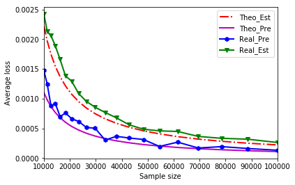
(a) KL-prediction and estimation losses

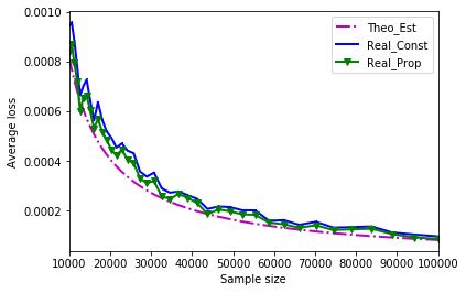
(b) $L_{2}$-estimation losses for different estimators

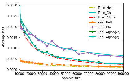
(c) Hellinger, Chi-squared, and Alpha- estimation losses

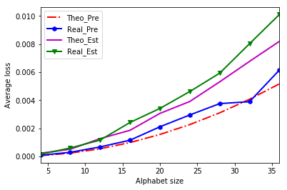
(d) Fixed $n$ and varying $k$

Figure 1: Experiments

8 Conclusions

We studied the problem of learning an unknown $k$-state Markov chain from its $n$ sequential sample points. We considered two formulations: prediction and estimation. For prediction, we determined the minimax risk up to a multiplicative factor of $k$. For estimation, when the transition probabilities are bounded away from zero, we obtained nearly matching lower and upper bounds on the minimax risk for $L_{2}$ and ordinary $f$-divergences. The effectiveness of our proposed estimators was verified through experimental simulations. Future directions include closing the gap in the prediction problem in Section 1, extending the results on the min-max estimation problem to other classes of Markov chains, and extending the work from the classical setting $k\ll n$, to general $k$ and $n$.

9 Minimax prediction: lower bound

A standard argument for lower bounding the minimax prediction risk is

$$\rho_{n}^{\text{KL}}(\mathscr{P})=\min_{\hat{P}}\max_{P\in\mathscr{P}}\rho_{n}^{\text{KL}}(P,\hat{P})\geq{\min_{\hat{P}}\mathds{E}_{P\sim\Pi}[\rho_{n}^{\text{KL}}(P,\hat{P})]},$$

where $\Pi$ is a prior distribution over $\mathscr{P}$. The advantage of this approach is that the optimal estimator that minimizes $\mathds{E}_{P\sim\Pi}[\rho_{n}^{\text{KL}}(P,\hat{P})]$ can often be computed explicitly.

Perhaps the simplest prior is the uniform distribution over some subset of $\mathscr{P}$. Consider the uniform distribution over $\mathscr{P}_{S}\subset\mathscr{P}$, say $U(\mathscr{P}_{S})$, the following lemma shows an explicit way of computing the optimal estimator for $\mathds{E}_{P\sim U(\mathscr{P}_{S})}[\rho_{n}^{\text{KL}}(P,\hat{P})]$ when $\mathscr{P}_{S}$ is finite.

Lemma 3.

Let $\hat{P}^{*}$ be the optimal estimator that minimizes $\mathds{E}_{P\sim U(\mathscr{P}_{S})}[\rho_{n}^{\text{KL}}(P,\hat{P})]$, then for any $x^{n}\in[k]^{n}$ and any symbol $i\in[k]$,

$$\hat{P}^{*}_{x^{n}}(i)=\sum_{P\in\mathscr{P}_{S}}\frac{P({x^{n}})}{\sum_{P^{\prime}\in\mathscr{P}_{S}}P^{\prime}({x^{n}})}P_{x^{n}}(i).$$

Clearly, computing $\hat{P}^{*}$ for all the possible sample sequences $x^{n}$ may be unrealistic. Instead, let ${\mathscr{K}}_{n}$ be an arbitrary subset of $[k]^{n}$, we can lower bound

$$\rho_{n}^{\text{KL}}(P,\hat{P})=\mathds{E}_{X^{n}\sim P}[D_{\text{KL}}(P_{X^{n}},\hat{P}_{X^{n}})]$$

by

$$\rho_{n}^{\text{KL}}(P,\hat{P};\mathscr{K}_{n}):=\mathds{E}_{X^{n}\sim P}[D_{\text{KL}}(P_{X^{n}},\hat{P}_{X^{n}})\mathds{1}_{X^{n}\in\mathscr{K}_{n}}].$$

This yields

$$\rho_{n}^{\text{KL}}(\mathscr{P})\geq{\min_{\hat{P}}\mathds{E}_{P\sim U(\mathscr{P}_{S})}[\rho_{n}^{\text{KL}}(P,\hat{P};\mathscr{K}_{n})]}.$$

The key to apply the above arguments is to find a proper pair $(\mathscr{P}_{S},\mathscr{K}_{n})$. The rest of this section is organized as follows. In Subsection 9.1, we present our construction of $\mathscr{P}_{S}$ and $\mathscr{K}_{n}$. In Subsection 9.2, we find the exact form of the optimal estimator using Lemma 3. Then we analyze its prediction risk over $\mathscr{K}_{n}$ in Subsection 9.3, where we further partition $\mathscr{K}_{n}$ into smaller subsets $K_{\ell}(i)$, and lower bound the KL-divergence over $K_{\ell}(i)$ and the probability $P(X^{n}\in K_{\ell}(i))$ in Lemma 6 and 7, respectively. Finally, we consolidate all the previous results and prove the desired lower bound on $\rho_{n}^{\text{KL}}(\mathscr{P})$.

9.1 Prior construction

Without loss of generality, we assume that $k$ is an even integer. For notational convenience, we denote by $u_{k}$ the uniform distribution over $[k]$ and define

$$M_{n}(p_{2},p_{4},\ldots,p_{k}):=\begin{bmatrix}b-a&a&a&a&\dots&a&a\\ p_{2}&b\!\!-\!\!p_{2}&a&a&\dots&a&a\\ a&a&b-a&a&\dots&a&a\\ a&a&p_{4}&b\!\!-\!\!p_{4}&\dots&a&a\\ \vdots&\vdots&\vdots&\vdots&\ddots&\vdots&\vdots\\ a&a&a&a&\dots&b-a&a\\ a&a&a&a&\dots&p_{k}&b\!\!-\!\!p_{k}\end{bmatrix},$$

where $a:=\frac{1}{n}$ and $b:=1-\frac{k-2}{n}$. In addition, let

$$V_{n}:=\left\{\frac{1}{\log^{t}n}:t\in\mathds{N}\text{ and }1\leq t\leq\frac{\log n}{2\log\log n}\right\}.$$

Given $n$, we set

$$\mathscr{P}_{S}=\{(M)\in{\mathds{M}}^{k}:\mu=u_{k}\text{ and }M=M_{n}(p_{2},p_{4},\ldots,p_{k}),\text{ where }p_{i}\in V_{n},\forall i\in[k]^{e}\}.$$

Then, we choose $\mathscr{K}_{n}$ to be the collection of sequences $x^{n}\in[k]^{n}$ whose last appearing state didn’t transition to any other symbol. In other words, for any state $i\in[k]$, let $\bar{i}$ represent an arbitrary state other than $i$, then

$$\mathscr{K}_{n}=\{x^{n}\in[k]^{n}:x^{n}={\bar{i}}^{n-\ell}i^{\ell}:i\in[k],n-1\geq\ell\geq{1}\}.$$

According to both the last appearing state and the number of times it transitions to itself, we can partition $\mathscr{K}_{n}$ as

$$\mathscr{K}_{n}=\cup_{\ell=1}^{n-1}K_{\ell}(i),\text{ where }K_{\ell}(i):=\{x^{n}\in[k]^{n}:x^{n}={\bar{i}}^{n-\ell}i^{\ell}\}.$$

9.2 The optimal estimator

Let $\hat{P}^{*}$ denote the optimal estimator that minimizes $\mathds{E}_{P\sim U(\mathscr{P}_{S})}[\rho_{n}^{\text{KL}}(P,\hat{P};\mathscr{K}_{n})]$. The following lemma presents the exact form of $\hat{P}^{*}$.

Lemma 4.

For any $x^{n}\in\mathscr{K}_{n}$, there exists a unique $K_{\ell}(i)$ that contains it. Consider $\hat{P}^{*}_{x^{n}}$, we have:

1. If $i\in[k]^{e}$, then

   $$\hat{P}^{*}_{x^{n}}(j):=\begin{cases}a&j>i\text{ or }j<i-1\\ \sum_{v\in V_{n}}(b-v)^{\ell}/\sum_{v\in V_{n}}(b-v)^{\ell-1}&j=i\\ \sum_{v\in V_{n}}(b-v)^{\ell-1}v/\sum_{v\in V_{n}}(b-v)^{\ell-1}&j=i-1\end{cases}$$

2. If $i\in[k]^{o}$, then

   $$\hat{P}^{*}_{x^{n}}(j):=\begin{cases}a&j>i\text{ or }j<i\\ b-a&j=i\end{cases}$$

Proof.

Given $(M)\in\mathscr{P}_{S}$, consider $X^{n}\sim(M)$,

$$\Pr(X^{n}=x^{n}) =\frac{1}{k}{\displaystyle\prod_{i_{1}\in[k]}{\prod_{j_{1}\in[k]}}M_{i_{1}j_{1}}^{N_{i_{1}j_{1}}}}.$$

By Lemma 3, for any $x^{n}\in{K_{\ell}(i)}$ and $j\in[k]$, $\hat{P}^{*}_{x^{n}}(j)$ evaluates to

$$\hat{P}^{*}_{x^{n}}(j) =\frac{\displaystyle\sum_{(M)\in\mathscr{P}_{S}}{M_{ij}}\prod_{i_{1}\in[k]}{\prod_{j_{1}\in[k]}}M_{i_{1}j_{1}}^{N_{i_{1}j_{1}}}}{\displaystyle\sum_{(M)\in\mathscr{P}_{S}}\prod_{i_{1}\in[k]}{\prod_{j_{1}\in[k]}}M_{i_{1}j_{1}}^{N_{i_{1}j_{1}}}}.$$

Noting that $x^{n}\in{K_{\ell}(i)}$ implies $N_{ii}=\ell-1$ and $N_{ij}=0,\forall j\not=i$. Besides, for any $j_{1}\in[k]$ and $i_{1}\in[k]\setminus{\{j_{1},j_{1}+1\}}$, $M_{i_{1}j_{1}}$ is uniquely determined by $i_{1}$ and $j_{1}$ for all $(M)\in\mathscr{P}_{S}$.

Thus, for $s=0$ or $1$, we can rewrite ${M_{ij}}^{s}\prod_{i_{1}\in[k]}{\prod_{j_{1}\in[k]}}M_{i_{1}j_{1}}^{N_{i_{1}j_{1}}}$ as

$C(x^{n},k){\displaystyle{M_{ij}^{s}}\prod_{\begin{subarray}{c}t=2\\ t\ even\end{subarray}}^{k}}\left[M_{t(t-1)}\right]^{N_{t(t-1)}}[M_{tt}]^{N_{tt}}$,

where $C(x^{n},k)$ is a constant that only depends on $x^{n}$ and $k$.

Hence, for any $x^{n}\in{K_{\ell}(i)}$,

$$\hat{P}^{*}_{x^{n}}(j) =\frac{\displaystyle\sum_{(M)\in\mathscr{P}_{S}}{\displaystyle{M_{ij}}\prod_{\begin{subarray}{c}t=2\\ t\ even\end{subarray}}^{k}}\left[M_{t(t-1)}\right]^{N_{t(t-1)}}[M_{tt}]^{N_{tt}}}{\displaystyle\sum_{(M)\in\mathscr{P}_{S}}{\displaystyle\prod_{\begin{subarray}{c}t=2\\ t\ even\end{subarray}}^{k}}\left[M_{t(t-1)}\right]^{N_{t(t-1)}}[M_{tt}]^{N_{tt}}}.$$

Below we show how to evaluate $\hat{P}^{*}_{x^{n}}(j)$ for $j=i\in[k]^{e}$, and other cases can be derived similarly.

Combining ${M_{jj}}^{N_{jj}}$ with $M_{jj}$ in the nominator,

$$\hat{P}^{*}_{x^{n}}(j) =\frac{\displaystyle\sum_{(M)\in\mathscr{P}_{S}}{\displaystyle{\left[M_{jj}^{\ell}\right]}\prod_{\begin{subarray}{c}t=2\\ t\ even\\ t\not=j\end{subarray}}^{k}}\left[M_{t(t-1)}\right]^{N_{t(t-1)}}[M_{tt}]^{N_{tt}}}{\displaystyle\sum_{(M)\in\mathscr{P}_{S}}{\displaystyle{\left[M_{jj}^{\ell-1}\right]}\prod_{\begin{subarray}{c}t=2\\ t\ even\\ t\not=j\end{subarray}}^{k}}\left[M_{t(t-1)}\right]^{N_{t(t-1)}}[M_{tt}]^{N_{tt}}}$$

$$=\frac{\displaystyle\sum_{\begin{subarray}{c}v\in{V_{n}}\\ v^{\prime}\in{V_{n}}\end{subarray}}{\displaystyle{(b-v^{\prime})^{\ell}}\prod_{\begin{subarray}{c}t=2\\ t\ even\\ t\not=j\end{subarray}}^{k}}v^{N_{t(t-1)}}(b-v)^{N_{tt}}}{\displaystyle\sum_{\begin{subarray}{c}v\in{V_{n}}\\ v^{\prime}\in{V_{n}}\end{subarray}}{\displaystyle{(b-v^{\prime})^{\ell-1}}\prod_{\begin{subarray}{c}t=2\\ t\ even\\ t\not=j\end{subarray}}^{k}}v^{N_{t(t-1)}}(b-v)^{N_{tt}}}$$

$$=\frac{{\left[\sum_{\begin{subarray}{c}v^{\prime}\in{V_{n}}\end{subarray}}(b-v^{\prime})^{\ell}\right]}\displaystyle\sum_{\begin{subarray}{c}v\in{V_{n}}\end{subarray}}{\displaystyle\prod_{\begin{subarray}{c}t=2\\ t\ even\\ t\not=j\end{subarray}}^{k}}v^{N_{t(t-1)}}(b-v)^{N_{tt}}}{{\left[\sum_{\begin{subarray}{c}v^{\prime}\in{V_{n}}\end{subarray}}(b-v^{\prime})^{\ell-1}\right]}\displaystyle\sum_{\begin{subarray}{c}v\in{V_{n}}\end{subarray}}{\displaystyle\prod_{\begin{subarray}{c}t=2\\ t\ even\\ t\not=j\end{subarray}}^{k}}v^{N_{t(t-1)}}(b-v)^{N_{tt}}}$$

$$=\frac{\sum_{\begin{subarray}{c}v\in{V_{n}}\end{subarray}}(b-v)^{\ell}}{\sum_{\begin{subarray}{c}v\in{V_{n}}\end{subarray}}(b-v)^{\ell-1}}.$$

This completes the proof. ∎

9.3 Analysis

Next, for any $x^{n}\in{K_{\ell}(i)}$, we lower bound $D_{\text{KL}}(P_{x^{n}},\hat{P}^{*}_{x^{n}})$ in terms of $M_{i(i-1)}$ and $\hat{P}^{*}_{x^{n}}(i-1)$.

Lemma 5.

For any $(M)\in\mathscr{P}_{S}$ and $x^{n}\in{K_{\ell}(i)}$,

$$D_{\text{KL}}(P_{x^{n}},\hat{P}^{*}_{x^{n}})\geq M_{i(i-1)}{\left({-1+\log\frac{M_{i(i-1)}}{\hat{P}^{*}_{x^{n}}(i-1)}}\right)}.$$

Proof.

By the previous lemma,

$$D_{\text{KL}}(P_{x^{n}},\hat{P}^{*}_{x^{n}})=M_{ii}\log\frac{M_{ii}}{\hat{P}^{*}_{x^{n}}(i)}+M_{i(i-1)}\log\frac{M_{i(i-1)}}{\hat{P}^{*}_{x^{n}}(i-1)}.$$

Noting that $\frac{x}{x+1}\leq\log(x+1)$ for all $x>-1$,

$$M_{ii}\log\frac{M_{ii}}{\hat{P}^{*}_{x^{n}}(i)} =M_{ii}\log{\left({\frac{M_{ii}-\hat{P}^{*}_{x^{n}}(i)}{\hat{P}^{*}_{x^{n}}(i)}+1}\right)}$$

$$\geq M_{ii}-\hat{P}^{*}_{x^{n}}(i)$$

$$={\left({b-M_{i(i-1)}}\right)}-{\left({b-\hat{P}^{*}_{x^{n}}{(i-1)}}\right)}$$

$$\geq-M_{i(i-1)}.$$

This completes the proof. ∎

Let $V^{\prime}_{n}:=\{\frac{1}{(\log n)^{t}}\ \mid t\in\mathds{N},1\leq{t}\leq{\frac{\log n}{4\log\log n}\}}$ be a subset of $V_{n}$ whose size is $\frac{1}{2}|V_{n}|$. For $M_{i(i-1)}\in V^{\prime}_{n}$, we further lower bound ${M_{i(i-1)}}/{\hat{P}^{*}_{x^{n}}(i-1)}$ in terms of $n$.

Let $\ell_{1}(M):=\frac{1}{M_{i(i-1)}}\frac{1}{\log\log n}$ and $\ell_{2}(M):={\frac{1}{M_{i(i-1)}}\log\log n}$, we have

Lemma 6.

For any $(M)\in\mathscr{P}_{S}$, $x^{n}\in{K_{\ell}(i)}$ where $i\in[k]^{e}$, $M_{i(i-1)}=\frac{1}{(\log n)^{m}}\in V^{\prime}_{n}$, and sufficiently large $n$, if

$$\ell_{1}(M)\leq\ell\leq\ell_{2}(M),$$

then,

$$\frac{M_{i(i-1)}}{\hat{P}^{*}_{x^{n}}(i-1)}\gtrsim\frac{\log n}{8\log\log n}(1-o(1)).$$

Proof.

Consider $M_{i(i-1)}=\frac{1}{(\log n)^{m}}\in V^{\prime}_{n}$, where $m\in[1,\frac{\log n}{4\log\log n}]$.

Note that for $x^{n}\in{K_{\ell}(i)}$, the value of $\hat{P}^{*}_{x^{n}}(i-1)$ only depends on $\ell$, we can define

$$F_{\ell}:=\frac{M_{i(i-1)}}{\hat{P}^{*}_{x^{n}}(i-1)}.$$

We have

$$F_{\ell}\geq\frac{A_{\ell}+X_{\ell}+C_{\ell}}{B_{\ell}+X_{\ell}+D_{\ell}},$$

where

$$X_{\ell}:={\left({1-\frac{k-2}{n}-\frac{1}{(\log{n})^{m}}}\right)}^{\ell},$$

$$A_{\ell}:=\sum\limits_{i=1}^{m-1}{{\left({1-\frac{k-2}{n}-\frac{1}{(\log{n})^{i}}}\right)}^{\ell}},$$

$$C_{\ell}:=\sum\limits_{i=m+1}^{\frac{\log n}{2\log\log n}}{{\left({1-\frac{k-2}{n}-\frac{1}{(\log{n})^{i}}}\right)}^{\ell}},$$

$$B_{\ell}:=\sum\limits_{i=1}^{m-1}{{\left({1-\frac{k-2}{n}-\frac{1}{(\log{n})^{i}}}\right)}^{\ell}}{(\log n)^{m-i}},$$

$$\text{ and }D_{\ell}:=\sum\limits_{i=m+1}^{\frac{\log n}{2\log\log n}}{{\left({1-\frac{k-2}{n}-\frac{1}{(\log{n})^{i}}}\right)}^{\ell}}{(\log n)^{m-i}}.$$

We have the following bounds on these quantities.

Bounds for $X_{\ell}$

$$0\leq X_{\ell}={\left({1-\frac{k-2}{n}-\frac{1}{(\log{n})^{m}}}\right)}^{\ell}\leq 1.$$

Bounds for $A_{\ell}$

$$0\leq A_{\ell}=\sum\limits_{i=1}^{m-1}{{\left({1-\frac{k-2}{n}-\frac{1}{(\log{n})^{i}}}\right)}^{\ell}}.$$

Bounds for $D_{\ell}$

$$0\leq D_{\ell}\leq{\sum\limits_{i=m+1}^{\frac{\log n}{2\log\log n}}{{\left({1-\frac{k-2}{n}-\frac{1}{(\log{n})^{i}}}\right)}^{\ell}}{\frac{1}{\log n}}}={\frac{1}{\log n}C_{\ell}}.$$

Bounds for $C_{\ell}$

Note that

$$\frac{(\log n)^{m}}{\log\log n}\leq\ell\leq{(\log n)^{m}\log\log n}$$

and

$$(\log n)^{m}\leq\sqrt{n}.$$

Consider a single term of $C_{\ell}$, we have

$${\left({1-\frac{k-2}{n}-\frac{1}{(\log n)^{i}}}\right)}^{\ell} \geq{{\left({1-\frac{k-2}{n}-\frac{1}{(\log n)^{i}}}\right)}^{(\log n)^{m}\log\log n}}$$

$$={{\left({1-\frac{k-2}{n}-\frac{1}{(\log n)^{i}}}\right)}^{\frac{1}{\frac{k-2}{n}+\frac{1}{(\log n)^{i}}}{\left({\frac{k-2}{n}+\frac{1}{(\log n)^{i}}}\right)}{\left({\log n}\right)}^{m}\log\log n}}$$

$$\geq{\left[\left(1-\frac{k-2}{n}-\frac{1}{(\log n)^{i}}\right)^{\frac{1}{\frac{k-2}{n}+\frac{1}{(\log n)^{i}}}}\right]^{(\frac{k-2}{\sqrt{n}}+\frac{1}{\log n})\log\log n}}$$

$$\geq{{\left({\frac{1}{4}}\right)}^{\frac{(k-2)\log\log n}{\sqrt{n}}+\frac{\log\log n}{\log n}}}$$

$$\geq{{\left({\frac{1}{4}}\right)}^{\frac{1}{2}}}=\frac{1}{2},$$

where we use the inequality $i\geq m+1$ and $(1-\frac{1}{x})^{x}\geq{\frac{1}{4}}$ for $x\geq{2}$.

Hence,

$${\frac{\log n}{8\log\log n}}={\frac{\log n}{4\log\log n}\cdot\frac{1}{2}}\leq C_{\ell}=\sum\limits_{i=m+1}^{\frac{\log n}{2\log\log n}}{{\left({1\!\!-\!\!\frac{k-2}{n}\!\!-\!\!\frac{1}{(\log{n})^{i}}}\right)}^{\ell}}\leq{\sum\limits_{i=m+1}^{\frac{\log n}{2\log\log n}}{1}}\leq{\frac{\log n}{2\log\log n}}.$$

Bounds for $B_{\ell}$

Similarly, consider a single term of $B_{\ell}$ without the factor $(\log n)^{m-i}$,

$${\left({1-\frac{k-2}{n}-\frac{1}{(\log n)^{i}}}\right)}^{\ell} \leq{{\left({1-\frac{k-2}{n}-\frac{1}{(\log{n})^{i}}}\right)}}^{\frac{(\log{n})^{m}}{\log{\log{n}}}}$$

$$\leq{{\left({1-\frac{k-2}{n}-\frac{1}{(\log{n})^{i}}}\right)}}^{\frac{1}{\frac{1}{(\log)^{i}}+\frac{k-2}{n}}{\left({\frac{1}{(\log)^{i}}+\frac{k-2}{n}}\right)}\frac{(\log{n})^{m}}{\log{\log{n}}}}$$

$$\leq{\left[\left(1-\frac{k-2}{n}-\frac{1}{(\log{n})^{i}}\right)^{\frac{1}{\frac{1}{(\log)^{i}}+\frac{k-2}{n}}}\right]^{{\left({\frac{1}{(\log)^{i}}+\frac{k-2}{n}}\right)}\frac{(\log{n})^{m}}{\log{\log{n}}}}}$$

$$\leq{{\left({\frac{1}{e}}\right)}^{\frac{(\log n)^{m-i}}{\log{\log{n}}}}}$$

$$={\left({\frac{1}{n}}\right)}^{\frac{(\log n)^{m-i-1}}{\log{\log{n}}}},$$

where we use the inequality $(1-\frac{1}{x})^{x}\leq{\frac{1}{e}}$ for $x\geq{2}$.

Hence,

$$B_{\ell} =\sum\limits_{i=1}^{m-1}{{\left({1-\frac{k-2}{n}-\frac{1}{(\log{n})^{i}}}\right)}^{\ell}}{(\log n)^{m-i}}$$

$$\leq{\sum\limits_{i=1}^{m-1}{\left({\frac{1}{n}}\right)}^{\frac{(\log n)^{m-i-1}}{\log{\log{n}}}}{(\log n)^{m-i}}}$$

$$=\sum\limits_{i=1}^{m-1}{\left({\frac{1}{n}}\right)}^{\frac{(\log n)^{m-i-1}}{3\log{\log{n}}}}{(\log n)^{m-i}}{\left({\frac{1}{n}}\right)}^{\frac{2(\log n)^{m-i-1}}{3\log{\log{n}}}}$$

$$={{\left({\frac{1}{n}}\right)}^{\frac{1}{\log{\log{n}}}}\log n+\sum\limits_{i=1}^{m-2}{\left({\frac{1}{n}}\right)}^{\frac{(\log n)^{m-i-1}}{3\log{\log{n}}}}{(\log n)^{m-i}}{\left({\frac{1}{n}}\right)}^{\frac{2(\log n)^{m-i-1}}{3\log{\log{n}}}}}$$

$$\leq{{\left({\frac{1}{n}}\right)}^{\frac{1}{\log{\log{n}}}}\log n+\sum\limits_{i=1}^{m-2}{\left({\frac{1}{n}}\right)}^{\frac{\log n}{3\log{\log{n}}}}{(\log n)^{m}}{\left({\frac{1}{n}}\right)}^{\frac{2\log n}{3\log{\log{n}}}}}$$

$$\leq{{\left({\frac{1}{n}}\right)}^{\frac{1}{\log{\log{n}}}}\log n+\sum\limits_{i=1}^{m-2}{\left({\frac{1}{n}}\right)}^{\frac{\log n}{3\log{\log{n}}}}{(\log n)^{\frac{\log n}{4\log{\log{n}}}}}{\left({\frac{1}{n}}\right)}^{\frac{2\log n}{3\log{\log{n}}}}}$$

$$\leq{{\left({\frac{1}{n}}\right)}^{\frac{1}{\log{\log{n}}}}\log n+\frac{\log n}{4\log{\log{n}}}{\left({\frac{1}{n}}\right)}^{\frac{\log n}{3\log{\log{n}}}}{(\log n)^{\frac{\log n}{4\log{\log{n}}}}}{\left({\frac{1}{n}}\right)}^{\frac{2\log n}{3\log{\log{n}}}}}$$

$$\leq{{\left({\frac{1}{n}}\right)}^{\frac{1}{\log{\log{n}}}}\log n+{\left({\frac{1}{n}}\right)}^{\frac{\log n}{3\log{\log{n}}}}{(\log n)^{\frac{\log n}{4\log{\log{n}}}+1}}{\left({\frac{1}{n}}\right)}^{\frac{2\log n}{3\log{\log{n}}}}}$$

$$\leq{{\left({\frac{1}{n}}\right)}^{\frac{1}{\log{\log{n}}}}e^{\log\log n}+{\left({\frac{\log{n}}{n}}\right)}^{\frac{\log n}{3\log{\log{n}}}}{\left({\frac{1}{n}}\right)}^{\frac{2\log n}{3\log{\log{n}}}}}$$

$$\leq{e^{\frac{-\log{n}+(\log{\log{n}})^{2}}{\log\log n}}+\frac{1}{n}}$$

$$\leq{e^{-\frac{2(\log{\log{n}})^{2}+(\log{\log{n}})^{2}}{\log\log n}}+\frac{1}{n}}$$

$$\leq{e^{-\log{\log{n}}}+\frac{1}{n}}$$

$$\leq{\frac{2}{\log{n}}},$$

where we use the inequality $x-2(\log{x})^{2}\geq{0}$ for $x\geq{1}$.

Putting everything together:

$$F_{\ell} =\frac{A_{\ell}+X_{\ell}+C_{\ell}}{B_{\ell}+X_{\ell}+D_{\ell}}\geq{\frac{0+\frac{\log n}{8\log\log n}}{\frac{2}{\log{n}}+1+\frac{1}{{2\log\log n}}}}\asymp\frac{\log n}{8\log\log n}.$$

This completes the proof. ∎

Another quantity that will be appear later is $\Pr(X^{n}\in K_{\ell}(i))$ where $X^{n}\sim(M)\in\mathscr{P}_{S}$. We need the following lower bound.

Lemma 7.

For $X^{n}\sim(M)\in\mathscr{P}_{S}$ and $i\in[k]^{e}$,

$$\Pr(X^{n}\in K_{\ell}(i))\gtrsim\frac{k-1}{ek}\frac{1}{n}{\left({1-\frac{k-2}{n}-M_{i(i-1)}}\right)}^{l-1}.$$

Proof.

By our construction of $\mathscr{P}_{S}$, for $X^{n}\sim(M)\in\mathscr{P}_{S}$ and $i\in[k]^{e}$, we have the following observations.

1. The probability that the initial state is not $i$ is $\frac{k-1}{k}$.

2. The probability of transitioning from some state $j\not=i$ to some state that is not $i$ is $1-\frac{1}{n}$.

3. The probability of transitioning from some state $j\not=i$ to state $i$ is $\frac{1}{n}$.

4. The probability of transitioning from state $i$ to itself is $1-\frac{k-2}{n}-M_{i(i-1)}$.

Therefore,

$$\Pr(X^{n}\in K_{\ell}(i)) =\frac{k-1}{k}{\left({1-\frac{1}{n}}\right)}^{n-\ell-1}\frac{1}{n}{\left({1-\frac{k-2}{n}-M_{i(i-1)}}\right)}^{\ell-1}$$

$$\geq\frac{k-1}{k}{\left({1-\frac{1}{n}}\right)}^{n}\frac{1}{n}{\left({1-\frac{k-2}{n}-M_{i(i-1)}}\right)}^{\ell-1}$$

$$\asymp\frac{k-1}{ek}\frac{1}{n}{\left({1-\frac{k-2}{n}-M_{i(i-1)}}\right)}^{\ell-1}.$$

This completes the proof. ∎

Now we turn back to $\rho_{n}^{\text{KL}}(\mathscr{P})$. According to the previous derivations,

$$\rho_{n}^{\text{KL}}(\mathscr{P}) \geq{\min_{\hat{P}}\mathds{E}_{P\sim U(\mathscr{P}_{S})}[\rho_{n}^{\text{KL}}(P,\hat{P};\mathscr{K}_{n})]}$$

$$=\mathds{E}_{P\sim U(\mathscr{P}_{S})}\left[\sum_{x^{n}\in\mathscr{K}_{n}}\Pr_{X^{n}\sim P}(X^{n}=x^{n})D_{\text{KL}}(P_{x^{n}},\hat{P}^{*}_{x^{n}})\right]$$

$$=\frac{1}{|\mathscr{P}_{S}|}\sum\limits_{(M)\in\mathscr{P}_{S}}\sum\limits_{l=1}^{n-1}\sum\limits_{i\in[k]}\sum\limits_{x^{n}\in{K_{\ell}(i)}}\left[\Pr_{X^{n}\sim P}(X^{n}=x^{n})D_{\text{KL}}(P_{x^{n}},\hat{P}^{*}_{x^{n}})\right]$$

$$\geq\frac{1}{|\mathscr{P}_{S}|}\sum\limits_{(M)\in\mathscr{P}_{S}}\sum\limits_{\ell=\ell_{1}(M)}^{\ell_{2}(M)}\sum\limits_{i\in[k]^{e}}\sum\limits_{x^{n}\in{K_{\ell}(i)}}\left[\Pr_{X^{n}\sim P}(X^{n}=x^{n})D_{\text{KL}}(P_{x^{n}},\hat{P}^{*}_{x^{n}})\right].$$

Noting that all $x^{n}\in{K_{\ell}(i)}$ have the same $P_{x^{n}}$ and $\hat{P}^{*}_{x^{n}}$, thus, the last formula can be written as

$$\frac{1}{|\mathscr{P}_{S}|}\sum\limits_{(M)\in\mathscr{P}_{S}}\sum\limits_{\ell=\ell_{1}(M)}^{\ell_{2}(M)}\sum\limits_{i\in[k]^{e}}\left[\Pr_{X^{n}\sim P}(X^{n}\in{K_{\ell}(i)})D_{\text{KL}}(P_{x^{n}},\hat{P}^{*}_{x^{n}};x^{n}\in{K_{\ell}(i)})\right].$$

By Lemma 5 and 6, for $\ell_{1}(M)\leq\ell\leq\ell_{2}(M)$ and $M_{i(i-1)}\in V^{\prime}_{n}$,

$$D_{\text{KL}}(P_{x^{n}},\hat{P}^{*}_{x^{n}};x^{n}\in{K_{\ell}(i)}) \geq M_{i(i-1)}{\left({-1+\log\frac{M_{i(i-1)}}{\hat{P}^{*}_{x^{n}}(i-1)}}\right)}$$

$$\gtrsim M_{i(i-1)}{\left({-1+\log{\left({\frac{\log n}{8\log\log n}}\right)}}\right)}$$

$$\asymp M_{i(i-1)}\log\log n.$$

By Lemma 7,

$$\Pr(X^{n}\in K_{\ell}(i))\gtrsim\frac{k-1}{ek}\frac{1}{n}{\left({1-\frac{k-2}{n}-M_{i(i-1)}}\right)}^{\ell-1}.$$

Therefore,

$$\rho_{n}^{\text{KL}}(\mathscr{P}) \geq\frac{1}{|\mathscr{P}_{S}|}\sum\limits_{(M)\in\mathscr{P}_{S}}\sum\limits_{\ell=\ell_{1}(M)}^{\ell_{2}(M)}\sum\limits_{i\in[k]^{e}}\left[\Pr_{X^{n}\sim P}(X^{n}\in{K_{\ell}(i)})D_{\text{KL}}(P_{x^{n}},\hat{P}^{*}_{x^{n}};x^{n}\in{K_{\ell}(i)})\right]$$

$$\gtrsim\frac{(k-1)\log\log n}{enk}\sum\limits_{i\in[k]^{e}}\frac{1}{|\mathscr{P}_{S}|}\!\!\!\!\sum\limits_{\begin{subarray}{c}(M)\in\mathscr{P}_{S}\\ \text{ and }M_{i(i-1)}\in V_{n}^{\prime}\end{subarray}}\sum\limits_{\ell=\ell_{1}(M)}^{\ell_{2}(M)}{\left({1\!\!-\!\!\frac{k-2}{n}\!\!-\!\!M_{i(i-1)}}\right)}^{\ell-1}\!\!\!\!M_{i(i-1)}$$

$$\geq\frac{(k-1)\log\log n}{enk}\sum\limits_{i\in[k]^{e}}\frac{1}{|V_{n}|}\sum_{v\in V^{\prime}_{n}}\sum\limits_{\ell=\frac{1}{v}\frac{1}{\log\log n}}^{\frac{1}{v}\log\log n}{\left({1\!\!-\!\!\frac{k-2}{n}\!\!-\!\!v}\right)}^{\ell-1}v,$$

where the last step follows by symmetry.

Next, we show that for any $v=\frac{1}{(\log n)^{m}}\in V^{\prime}_{n}$,

$$T_{m}:=\sum\limits_{\ell=\frac{1}{v}\frac{1}{\log\log n}}^{\frac{1}{v}\log\log n}{\left({1-\frac{k-2}{n}-v}\right)}^{\ell-1}v\gtrsim 1.$$

Noting that $T_{m}$ is simply the summation of a geometric sequence, we can compute it as follows

$$\begin{split}T_{m}&=\frac{1}{(\log n)^{m}}\sum\limits_{\ell=\frac{(\log n)^{m}}{\log\log n}}^{(\log n)^{m}\log\log n}\left[\left(1-\frac{k-2}{n}-\frac{1}{(\log n)^{m}}\right)^{\ell-1}\right]\\ &=\frac{1}{(\log n)^{m}}\frac{\left(1\!\!-\!\!\frac{k-2}{n}\!\!-\!\!\frac{1}{(\log n)^{m}}\right)^{\frac{(\log n)^{m}}{\log\log n}-1}-\left(1\!\!-\!\!\frac{k-2}{n}\!\!-\!\!\frac{1}{(\log n)^{m}}\right)^{(\log n)^{m}\log\log n}}{1-\left(1\!\!-\!\!\frac{k-2}{n}\!\!-\!\!\frac{1}{(\log n)^{m}}\right)}\\ &=\frac{1}{\frac{(k-2)(\log{n})^{m}}{n}+1}\left[\left(1-\frac{k-2}{n}-\frac{1}{(\log n)^{m}}\right)^{\frac{(\log n)^{m}}{\log\log n}-1}\right.\\ &\left.-\left(1-\frac{k-2}{n}-\frac{1}{(\log n)^{m}}\right)^{(\log n)^{m}\log\log n}\right].\end{split}$$

To provide a lower bound for $T_{m}$, we use the following inequalities:

$$\frac{1}{\frac{(k-2)(\log{n})^{m}}{n}+1}\geq{\frac{1}{\frac{(k-2)(\log{n})^{\frac{\log n}{4\log\log n}}}{n}+1}}=\frac{1}{\frac{(k-2)n^{\frac{1}{4}}}{n}+1}\asymp 1,$$

$$\left(1\!\!-\!\!\frac{k-2}{n}\!\!-\!\!\frac{1}{(\log n)^{m}}\right)^{\frac{(\log n)^{m}}{\log\log n}-1} \geq\left[{\left(1\!\!-\!\!\frac{k-2}{n}\!\!-\!\!\frac{1}{(\log{n})^{m}}\right)}^{\frac{1}{\frac{1}{(\log)^{m}}+\frac{k-2}{n}}}\right]^{\left(1+\frac{(k-2)(\log{n})^{m}}{n}\right)\frac{1}{\log{\log{n}}}}$$

$$\geq{{\left({\frac{1}{4}}\right)}^{(1+\frac{(k-2)\sqrt{n}}{n})\frac{1}{\log{\log{n}}}}}\geq{{\left({\frac{1}{4}}\right)}^{2\frac{1}{\log{\log{n}}}}}\asymp 1,$$

and

$$\left(1\!\!-\!\!\frac{k-2}{n}\!\!-\!\!\frac{1}{(\log n)^{m}}\right)^{(\log n)^{m}\log\log n}$$

$$=\left[\left(1\!\!-\!\!\frac{k-2}{n}\!\!-\!\!\frac{1}{(\log n)^{m}}\right)^{\frac{1}{\frac{k-2}{n}+\frac{1}{(\log n)^{m}}}}\right]^{\left(\frac{(k-2)(\log{n})^{m}}{n}+1\right)\log\log n}$$

$$\leq{\left(\frac{1}{e}\right)^{\log\log n}}=\frac{1}{\log{n}}.$$

Consolidating these three inequalities, the sum $T_{m}$ can be lower bounded by

$$T_{m}\gtrsim{{1}}{(1-\frac{1}{\log{n}})}\asymp 1.$$

Finally,

$$\rho_{n}^{\text{KL}}(\mathscr{P}) \gtrsim\frac{(k-1)\log\log n}{enk}\sum\limits_{i\in[k]^{e}}\frac{1}{|V_{n}|}\sum_{v\in V^{\prime}_{n}}(1-o(1))$$

$$=\frac{(k-1)\log\log n}{enk}\frac{k}{2}\frac{|V^{\prime}_{n}|}{|V_{n}|}$$

$$=\frac{(k-1)\log\log n}{4en}.$$

10 Minimax prediction: upper bound

The proof makes use of the following lemma, which provides a uniform upper bound for the hitting probability of any $k$-state Markov chain.

Lemma 8.

sup17 For any Markov chain over $[k]$ and any two states $i,j\in[k]$, if $n>k$, then

$$\textrm{Pr}_{i}{(\tau(j)=n)}\leq\frac{k}{n}.$$

Let $\mathscr{K}_{n}$ be the same as is in the previous section. Recall that

$$\rho_{n}^{\text{KL}}(P,\hat{P};\mathscr{K}_{n})=\sum_{x^{n}\in\mathscr{K}_{n}}P(x^{n})D_{\text{KL}}(P_{x^{n}},\hat{P}_{x^{n}}),$$

we denote the partial minimax prediction risk over $\mathscr{K}_{n}$ by

$$\rho_{n}^{\text{KL}}(\mathscr{P};\mathscr{K}_{n}):=\min_{\hat{P}}\max_{P\in\mathscr{P}}\rho_{n}^{\text{KL}}(P,\hat{P};\mathscr{K}_{n}).$$

Let $\overline{\mathscr{K}_{n}}:=[k]^{n}\setminus\mathscr{K}_{n}$, we define $\rho_{n}^{\text{KL}}(P,\hat{P};\overline{\mathscr{K}_{n}})$ and $\rho_{n}^{\text{KL}}(\mathscr{P};\overline{\mathscr{K}_{n}})$ in the same manner. As the consequence of $\hat{P}$ being a function from $[k]^{n}$ to $\Delta_{k}$, we have the following triangle inequality,

$$\rho_{n}^{\text{KL}}(\mathscr{P})\leq\rho_{n}^{\text{KL}}(\mathscr{P};\overline{\mathscr{K}_{n}})+\rho_{n}^{\text{KL}}(\mathscr{P};\mathscr{K}_{n}).$$

Turning back to Markov chains, the next lemma upper bounds $\rho_{n}^{\text{KL}}({\mathds{M}}^{k};\overline{\mathscr{K}_{n}})$.

Lemma 9.

Let $\hat{P}^{+\frac{1}{2}}$ denote the estimator that maps $X^{n}\sim(M)$ to $\hat{M}^{+\frac{1}{2}}(X_{n},\cdot)$, then

$$\max_{P\in{\mathds{M}}^{k}}\rho_{n}^{\text{KL}}(P,\hat{P}^{+\frac{1}{2}};\overline{\mathscr{K}_{n}})\leq{\mathcal{O}_{k}\left(\frac{1}{n}\right)},$$

which implies

$$\rho_{n}^{\text{KL}}({\mathds{M}}^{k};\overline{\mathscr{K}_{n}})\leq{\mathcal{O}_{k}\left(\frac{1}{n}\right)}.$$

Proof.

The proof of this lemma is essentially a combination of the upper bounds’ proofs in Moein16 and in Section 12. Instead of using the fact that $M_{ij}$ are bounded away from $0$ (see Section 12), we partition $\overline{\mathscr{K}_{n}}$ into different subsets according to how close the counts are to their expected values, the number of times that the last appearing state transitioning to itself, and the number of times that the last appearing state transitioning to other states. Then, we bound the estimator’s expected loss over each set of the partition by ${\mathcal{O}_{k}\left({1}/{n}\right)}$. We omit the proof for the sake of brevity. ∎

Recall the following lower bound,

$$\rho_{n}^{\text{KL}}({\mathds{M}}^{k})=\Omega_{k}{\left({\frac{\log\log n}{n}}\right)}.$$

This together with Lemma 5 and the triangle inequality above shows that an upper bound on $\rho_{n}^{\text{KL}}({\mathds{M}}^{k};\mathscr{K}_{n})$ also suffices to bound the leading term of $\rho_{n}^{\text{KL}}({\mathds{M}}^{k})$. The following lemma provides such an upper bound. Recall that for any $i\in[k]$, $K_{\ell}(i)$ is defined as $\{x^{n}\in[k]^{n}:x^{n}={\bar{i}}^{n-\ell}i^{\ell}\}$.

Lemma 10.

For any $x^{n}\in\mathscr{K}_{n}$, there exists a unique pair $(\ell,i)$ such that $x^{n}\in K_{\ell}(i)$. Consider the following estimator

$$\hat{P}_{x^{n}}(i):=\begin{cases}1-\frac{1}{\ell\log n}&\ell\leq\frac{n}{2}\\ 1-\frac{1}{\ell}&\ell>\frac{n}{2}\end{cases}$$

and

$$\hat{P}_{x^{n}}(j):=\frac{1-\hat{P}_{x^{n}}(i)}{k-1},\ \forall j\in[k]\setminus\{i\},$$

then we have

$$\rho_{n}^{\text{KL}}({\mathds{M}}^{k};\mathscr{K}_{n})\leq\max_{P\in{\mathds{M}}^{k}}\rho_{n}^{\text{KL}}(P,\hat{P};\mathscr{K}_{n})\lesssim\frac{2k^{2}\log\log n}{n}.$$

Proof.

Let $i\in[k]$ be an arbitrary state. For simplicity of illustration, we use the following notation: for any $x^{n}={\bar{i}}^{n-\ell}i^{\ell}$, denote $\hat{p}_{\ell}:=\hat{P}_{x^{n}}$; for any $(M)\in{\mathds{M}}^{k}$, denote $p_{i}:=M(i,\cdot)$; for any $\ell\leq{n}$, denote $h_{i,\ell}:=\Pr(\tau(i)=\ell)$. By Lemma 8, the hitting probability $h_{i,\ell}$ is upper bounded by $k/\ell$ for all $\ell>k$. We can write

$$\rho_{n}^{\text{KL}}(P,\hat{P};\mathscr{K}_{n})=\sum_{i\in[k]}\sum_{\ell=1}^{n-1}h_{i,n-\ell}(p_{i}(i))^{\ell-1}D_{\text{KL}}(p_{i},\hat{p}_{\ell}).$$

Now, we break the right hand side into two sums according to whether $\ell$ is greater than $n/2$ or not. For $\ell>n/2$, we have

$$\sum_{i\in[k]}\sum_{\ell=\frac{n}{2}+1}^{n-1}h_{i,n-\ell}(p_{i}(i))^{\ell-1}D_{\text{KL}}(p_{i},\hat{p}_{\ell})$$

$$\leq\sum_{i\in[k]}\sum_{\ell=\frac{n}{2}+1}^{n-1}h_{i,n-\ell}(p_{i}(i))^{\ell-1}{\left({p_{i}(i)\log{\left({\frac{p_{i}(i)}{1-\frac{1}{\ell}}}\right)}+\sum_{j\not=i}p_{i}(j)\log{\left({\frac{\sum_{j\not=i}p_{i}(j)}{\frac{1}{\ell(k-1)}}}\right)}}\right)}$$

$$\leq\sum_{i\in[k]}\sum_{\ell=\frac{n}{2}+1}^{n-1}h_{i,n-\ell}(p_{i}(i))^{\ell-1}{\left({\log{\left({\frac{1}{1-\frac{1}{\ell}}}\right)}+(1-p_{i}(i))\log{\left({{\ell(k-1)(1-p_{i}(i))}}\right)}}\right)}$$

$$\leq\sum_{i\in[k]}\sum_{\ell=\frac{n}{2}+1}^{n-1}h_{i,n-\ell}(p_{i}(i))^{\ell-1}{\left({\frac{\frac{1}{\ell}}{1-\frac{1}{\ell}}+(1-p_{i}(i))^{2}{\ell(k-1)}}\right)}$$

$$\leq\sum_{i\in[k]}\sum_{\ell=\frac{n}{2}+1}^{n-1}h_{i,n-\ell}{\left({\frac{2}{n}+(p_{i}(i))^{\ell-1}(1-p_{i}(i))^{2}{\ell(k-1)}}\right)}$$

$$\leq\sum_{i\in[k]}\sum_{\ell=\frac{n}{2}+1}^{n-1}h_{i,n-\ell}{\left({\frac{2}{n}+\frac{1}{(\ell+1)^{2}}{\ell(k-1)}}\right)}$$

$$\leq\sum_{i\in[k]}\sum_{\ell=\frac{n}{2}+1}^{n-1}h_{i,n-\ell}{\left({\frac{2k}{n}}\right)}$$

$$=\sum_{i\in[k]}\frac{2k}{n}\Pr(\tau(i)\in[1,n/2-1])\leq\frac{2k^{2}}{n}.$$

Similarly, for $\ell\leq n/2$, we have

$$\sum_{i\in[k]}\sum_{\ell=1}^{\frac{n}{2}}h_{i,n-\ell}(p_{i}(i))^{\ell-1}D_{\text{KL}}(p_{i},\hat{p}_{\ell})$$

$$\leq\sum_{i\in[k]}\sum_{\ell=1}^{\frac{n}{2}}h_{i,n-\ell}(p_{i}(i))^{\ell-1}{\left({\log{\left({\frac{1}{1-\frac{1}{\ell\log n}}}\right)}+(1-p_{i}(i))\log{\left({{\ell(k-1)(1-p_{i}(i))\log n}}\right)}}\right)}$$

$$\leq\sum_{i\in[k]}\sum_{\ell=1}^{\frac{n}{2}}\frac{2k}{n}(p_{i}(i))^{\ell-1}{\left({\frac{2}{\ell\log n}+(1-p_{i}(i))^{2}{\ell(k-1)}+(1-p_{i}(i))\log\log n}\right)}$$

$$\leq\sum_{i\in[k]}\frac{2k}{n}{\left({\sum_{\ell=1}^{\frac{n}{2}}\frac{2}{\ell\log n}+\sum_{\ell=1}^{\frac{n}{2}}\ell(p_{i}(i))^{\ell-1}(1-p_{i}(i))^{2}{(k-1)}+\sum_{\ell=1}^{\frac{n}{2}}(p_{i}(i))^{\ell-1}(1-p_{i}(i))\log\log n}\right)}$$

$$\leq\sum_{i\in[k]}\frac{2k}{n}{\left({2+(k-1)+\log\log n}\right)}$$

$$\asymp\frac{2k^{2}\log\log n}{n}.$$

This completes the proof. ∎

11 Minimax estimation: lower bound

The proof of the lower bound makes use of the following concentration inequality, which upper bounds the probability that a binomial random variable exceeds its mean.

Lemma 11.

com06 Let $Y$ be a binomial random variable with parameters $m\in\mathds{N}$ and $p\in[0,1]$, then for any $\epsilon\in(0,1)$,

$$\textrm{Pr}{(Y\geq(1+\epsilon)mp)}\leq\exp\left(-\epsilon^{2}mp/3\right).$$

11.1 Prior construction

Again we use the following standard argument to lower bound the minimax risk,

$$\varepsilon_{n}^{L}(\mathscr{M})=\min_{\hat{M}}\max_{(M)\in\mathscr{M}}\varepsilon_{n}^{L}(M,\hat{M})\geq{\min_{\hat{M}}\mathds{E}_{(M)\sim U(\mathscr{M}_{S})}[\varepsilon_{n}^{L}(M,\hat{M})]},$$

where $\mathscr{M}_{S}\subset\mathscr{M}$ and $U(\mathscr{M}_{S})$ is the uniform distribution over $\mathscr{M}_{S}$. Setting $\mathscr{M}={\mathds{M}}^{k}_{\delta,\pi^{*}}$, we outline the construction of $\mathscr{M}_{S}$ as follows.

We adopt the notation in KamathOPS15 and denote the $L_{\infty}$ ball of radius $r$ around $u_{k-1}$, the uniform distribution over $[k-1]$, by

$$B_{k-1}(r):=\{p\in\Delta_{k-1}:{L_{\infty}}(p,u_{k-1})<r\},$$

where ${L_{\infty}}(\cdot,\cdot)$ is the $L_{\infty}$ distance between two distributions. For simplicity, define

$$p^{\prime}:=(p_{1},\ p_{2},\ \ldots,\ p_{k-1}),$$

$$p^{*}:={\left({\frac{\bar{\pi}^{*}}{k-1},\ \frac{\bar{\pi}^{*}}{k-1},\ \dots\ \frac{\bar{\pi}^{*}}{k-1},\ \pi^{*}}\right)},$$

and

$$M_{n}(p^{\prime}):=\begin{bmatrix}\frac{\bar{\pi}^{*}}{k-1}&\frac{\bar{\pi}^{*}}{k-1}&\dots&\frac{\bar{\pi}^{*}}{k-1}&\pi^{*}\\ \frac{\bar{\pi}^{*}}{k-1}&\frac{\bar{\pi}^{*}}{k-1}&\dots&\frac{\bar{\pi}^{*}}{k-1}&\pi^{*}\\ \vdots&\vdots&\ddots&\vdots&\vdots\\ \frac{\bar{\pi}^{*}}{k-1}&\frac{\bar{\pi}^{*}}{k-1}&\dots&\frac{\bar{\pi}^{*}}{k-1}&\pi^{*}\\ \bar{\pi}^{*}p_{1}&\bar{\pi}^{*}p_{2}&\dots&\bar{\pi}^{*}p_{k-1}&\pi^{*}\end{bmatrix},$$

where $\bar{\pi}^{*}=1-\pi^{*}$ and $\sum_{i=1}^{k-1}p_{i}=1$.

Given $n$ and $\epsilon\in(0,1)$, let $n^{\prime}:=(n(1+\epsilon)\pi^{*})^{1/5}$. We set

$$\mathscr{M}_{S}=\{(M)\in{\mathds{M}}^{k}_{\delta,\pi^{*}}:\mu=p^{*}\text{ and }M=M_{n}({p^{\prime}}),\text{ where }p^{\prime}\in B_{k-1}(1/n^{\prime})\}.$$

Noting that the uniform distribution over $\mathscr{M}_{S}$, $U(\mathscr{M}_{S})$, is induced by $U(B_{k-1}(1/n^{\prime}))$, the uniform distribution over $B_{k-1}(1/n^{\prime})$ and thus is well-defined.

An important property of the above construction is that for a sample sequence $X^{n}\sim(M)\in\mathscr{M}_{S}$, $N_{k}$, the number of times that state $k$ appears in $X^{n}$, is a binomial random variable with parameters $n$ and $\pi^{*}$. Therefore, Lemma 11 implies that $N_{k}$ is highly concentrated around its mean $n\pi^{*}$.

11.2 $L_{2}$-divergence lower bound

Let us first consider the $L_{2}$-distance. Similar to Lemma 3, $\hat{M}^{*}$, the estimator that minimizes $\mathds{E}_{(M)\sim U(\mathscr{M}_{S})}[\varepsilon_{n}^{L_{2}}(M,\hat{M})]$, can be computed exactly. In particular, we have the following lemma.

Lemma 12.

There exists an estimator $\hat{M}^{*}$ with

$$\hat{M}^{*}_{x^{n}}(i,\cdot)=p^{*},\forall i\in[k-1],$$

and

$$\hat{M}^{*}_{x^{n}}(k,k)=\pi^{*},$$

such that $\hat{M}^{*}$ minimizes $\mathds{E}_{(M)\sim U(\mathscr{M}_{S})}[\varepsilon_{n}^{L_{2}}(M,\hat{M})]$.

Based on the above lemma, we can relate the minimax estimation risk of Markov chains to the minimax prediction risk of i.i.d. processes. For simplicity, denote $\mathscr{B}_{\textit{i.i.d.}}:=\{(p)\in\mathds{IID}^{k-1}:p\in B_{k-1}(1/n^{\prime})\}$. The following lemma holds.

Lemma 13.

For any $x^{n}\in[k]^{n}$, let $\mathds{I}(x^{n})$ be the collection of indexes $j\in[n]$ such that $x_{j}=k$. Then,

$${\mathds{E}}_{(M)\sim U(\mathscr{M}_{S})}[\mathds{E}_{X^{n}\sim(M)}[L_{2}(M(k,\cdot),\hat{M}^{*}_{X^{n}}(k,\cdot))\mathds{1}_{\mathds{I}(X^{n})=\mathds{I}_{0}}]]$$

$$=C{(\mathds{I}_{0},\pi^{*},p^{*},n)}\min_{\hat{P}}\mathds{E}_{P\sim U(\mathscr{B}_{\textit{i.i.d.}})}[\rho_{|\mathds{I}_{0}|}^{L_{2}}(P,\hat{P})],$$

where $\mathds{I}_{0}$ is an arbitrary non-empty subset of $[n]$ and $C{(\mathds{I}_{0},\pi^{*},p^{*},n)}$ is a constant whose value only depends on $\mathds{I}_{0},\pi^{*},p^{*},\text{ and }n$.

Proof.

We first consider the inner expectation on the left-hand side of the equality. For any $(M)\in\mathscr{M}_{S}$, we have

$$\mathds{E}_{X^{n}\sim(M)}[{L_{2}}(M(k,\cdot),\hat{M}^{*}_{X^{n}}(k,\cdot))\mathds{1}_{\mathds{I}(X^{n})=\mathds{I}_{0}}]$$

$$=\sum_{x^{n}:{\mathds{I}(x^{n})=\mathds{I}_{0}}}P(x^{n}){L_{2}}(M(k,\cdot),\hat{M}^{*}_{x^{n}}(k,\cdot))$$

$$=\sum_{x^{n}:{\mathds{I}(x^{n})=\mathds{I}_{0}}}\mu(x_{1})\prod_{t=1}^{n-1}M(x_{t},x_{t+1}){L_{2}}(M(k,\cdot),\hat{M}^{*}_{x^{n}}(k,\cdot)).$$

Let us partition $\mathds{I}_{0}$ into two parts: the collection of indexes $m\in\mathds{I}_{0}\cap[n-1]$ such that $m\in\mathds{I}_{0}$ and $m+1\not\in\mathds{I}_{0}$, say $\{m_{1},\ldots,m_{s}\}$, and the remaining elements in $\mathds{I}_{0}$. By the construction of $\mathscr{M}_{S}$, we have

$$\sum_{x^{n}:{\mathds{I}(x^{n})=\mathds{I}_{0}}}\mu(x_{1})\prod_{t=1}^{n-1}M(x_{t},x_{t+1}){L_{2}}(M(k,\cdot),\hat{M}^{*}_{x^{n}}(k,\cdot))$$

$$=(\pi^{*})^{|\mathds{I}_{0}|}{\left({\frac{\bar{\pi}^{*}}{k-1}}\right)}^{n-s-|\mathds{I}_{0}|}\sum_{x^{n}:{\mathds{I}(x^{n})=\mathds{I}_{0}}}\prod_{t=1}^{s}M(k,x_{m_{t}+1}){L_{2}}(M(k,\cdot),\hat{M}^{*}_{x^{n}}(k,\cdot)).$$

For any $x^{n}$, let $x^{n}\setminus\mathds{I}_{0}$ denote the subsequence $x_{j_{1}},\ldots,x_{j_{n-|\mathds{I}_{0}|-s}}$ such that $j_{1}<j_{2}\ldots<j_{n-|\mathds{I}_{0}|-s}$, $j_{t}\not\in\mathds{I}_{0}\text{ and }j_{t}-1\not\in\{m_{1},\ldots,m_{s}\},\forall t$. We can further partition the last summation according to $x^{n}\setminus\mathds{I}_{0}$ as follows.

$$\sum_{x^{n}:{\mathds{I}(x^{n})=\mathds{I}_{0}}}\prod_{t=1}^{s}M(k,x_{m_{t}+1}){L_{2}}(M(k,\cdot),\hat{M}^{*}_{x^{n}}(k,\cdot))$$

$$=\sum_{y^{n-|\mathds{I}_{0}|-s}\in[k-1]^{n-|\mathds{I}_{0}|-s}}{\left({\sum_{\begin{subarray}{c}x^{n}:{x_{j}=k,\forall j\in\mathds{I}_{0}}\\ \text{ and }x^{n}\setminus\mathds{I}_{0}=y^{n-|\mathds{I}_{0}|-s}\end{subarray}}\prod_{t=1}^{s}M(k,x_{m_{t}+1}){L_{2}}(M(k,\cdot),\hat{M}^{*}_{x^{n}}(k,\cdot))}\right)}.$$

Fixing $y^{n-|\mathds{I}_{0}|-s}\in[k-1]^{n-|\mathds{I}_{0}|-s}$, there is a bijective mapping from $S(\mathds{I}_{0},y^{n-|\mathds{I}_{0}|-s}):=\{x^{n}:{x_{j}=k,\forall j\in\mathds{I}_{0}}\text{ and }x^{n}\setminus\mathds{I}_{0}=y^{n-|\mathds{I}_{0}|-s}\}$ to $[k-1]^{s}$, say $g(\cdot)$. Furthermore, we have $\hat{M}^{*}(k,k)=\pi^{*}$. Hence, we can denote $q^{*}_{g(x^{n})}:=\frac{\hat{M}^{*}_{x^{n}}(k,[k-1])}{\bar{\pi}^{*}}$ for $x^{n}\in S(\mathds{I}_{0},y^{n-|\mathds{I}_{0}|-s})$ and treat it as a mapping from $[k-1]^{s}$ to $\Delta_{k-1}$. Also, $(M)\in\mathscr{M}_{S}$ implies that $M(k,[k-1])=p^{\prime}$ for some $p^{\prime}\in B_{k-1}(1/n^{\prime})$. Thus,

$${L_{2}}(M(k,\cdot),\hat{M}^{*}_{x^{n}}(k,\cdot))=(\bar{\pi}^{*})^{2}L_{2}(p^{\prime},q^{*}_{g(x^{n})}),$$

$$\prod_{t=1}^{s}M(k,x_{m_{t}+1})L_{2}(M(k,\cdot),\hat{M}^{*}_{x^{n}}(k,\cdot))=\prod_{t=1}^{s}p^{\prime}(x_{m_{t}+1})(\bar{\pi}^{*})^{2}L_{2}(p^{\prime},q^{*}_{g(x^{n})}),$$

and

$$\sum_{x^{n}\in S(\mathds{I}_{0},y^{n-|\mathds{I}_{0}|-s})}\prod_{t=1}^{s}M(k,x_{m_{t}+1})L_{2}(M(k,\cdot),\hat{M}^{*}_{x^{n}}(k,\cdot))$$

$$=\sum_{x^{n}\in S(\mathds{I}_{0},y^{n-|\mathds{I}_{0}|-s})}\prod_{t=1}^{s}p^{\prime}(x_{m_{t}+1})(\bar{\pi}^{*})^{2}L_{2}(p^{\prime},q^{*}_{g(x^{n})})$$

$$=\sum_{z^{s}\in[k-1]^{s}}\prod_{t=1}^{s}p^{\prime}(z_{t})(\bar{\pi}^{*})^{2}L_{2}(p^{\prime},q^{*}_{z^{s}})$$

$$=\mathds{E}_{Z^{s}\sim(p^{\prime})}[(\bar{\pi}^{*})^{2}L_{2}(p^{\prime},q^{*}_{Z^{s}})],$$

where $(p^{\prime})$ is an i.i.d. process whose underlying distribution is $p^{\prime}$.

By definition, $\hat{M}^{*}$ minimizes $\mathds{E}_{(M)\sim U(\mathscr{M}_{S})}[\varepsilon_{n}^{L_{2}}(M,\hat{M})]$ and for each $x^{n}\in[k]^{n}$, its value $\hat{M}^{*}_{x^{n}}$ is completely determined by $x^{n}$. Besides, $\{S(\mathds{I}_{0},y^{n-|\mathds{I}_{0}|-s}):\mathds{I}_{0}\subset[n]\text{ and }y^{n-|\mathds{I}_{0}|-s}\in[k-1]^{n-|\mathds{I}_{0}|-s}\}$ forms a partition of $[k]^{n}$. Therefore, by the linearity of expectation and the definition of $q^{*}$, the estimator $q^{*}$ also minimizes $\mathds{E}_{p^{\prime}\sim U(B_{k-1}(1/n^{\prime}))}[\mathds{E}_{Z^{s}\sim(p^{\prime})}[(\bar{\pi}^{*})^{2}L_{2}(p^{\prime},q_{Z^{s}})]]$, where the minimization is over all the possible mappings $q$ from $[k-1]^{s}$ to $\Delta_{k-1}$. Equivalently, we have

$$\mathds{E}_{p^{\prime}\sim U(B_{k-1}(1/n^{\prime}))}[\mathds{E}_{Z^{n}\sim(p^{\prime})}[(\bar{\pi}^{*})^{2}L_{2}(p^{\prime},q^{*}_{Z^{n}})]]=\min_{\hat{P}}\mathds{E}_{P\sim U(\mathscr{B}_{\textit{i.i.d.}})}(\bar{\pi}^{*})^{2}[\rho_{s}^{L_{2}}(P,\hat{P})].$$

This immediately yields the lemma. ∎

For any $(M)\in\mathscr{M}_{S}$, denote by $N_{k}((M),n)$ the number of times that state $k$ appears in $X^{n}\sim(M)$, which is a random variable induced by $(M)$ and $n$. Lemma 13, we can deduce that

Lemma 14.

$$\min_{\hat{M}}\mathds{E}_{(M)\sim U(\mathscr{M}_{S})}[\varepsilon_{n}^{L_{2}}(M,\hat{M})]\geq{\mathds{E}_{(M)\sim U(\mathscr{M}_{S})}\left[(\bar{\pi}^{*})^{2}\min_{\hat{P}}\mathds{E}_{P^{\prime}\sim U(\mathscr{B}_{\textit{i.i.d.}})}[\rho_{N_{k}((M),n)}^{L_{2}}(P^{\prime},\hat{P})]\right]}.$$

By Lemma 11 and our construction of $\mathscr{M}_{S}$, the probability that $N_{k}((M),n)\geq(1+\epsilon)n\pi^{*}$ is at most $\exp(-\epsilon^{2}n\pi^{*}/3)$ for any $(M)\in\mathscr{M}_{S}$ and $\epsilon\in(0,1)$. This together with Lemma 14 and

$$\min_{\hat{P}}\mathds{E}_{P\sim U(\mathscr{B}_{\textit{i.i.d.}})}[\rho_{m}^{L_{2}}(P,\hat{P})]\gtrsim{\frac{1-\frac{1}{k-1}}{(1+\epsilon)n\pi^{*}}},\forall m<(1+\epsilon)n\pi^{*},$$

from KamathOPS15 yields

Lemma 15.

For all $\epsilon\in(0,1)$,

$$\varepsilon_{n}^{L_{2}}(\mathscr{M})=\varepsilon_{n}^{L_{2}}({\mathds{M}}^{k}_{\delta,\pi^{*}})\gtrsim{\frac{(1-\frac{1}{k-1})(1-\pi^{*})^{2}}{n\pi^{*}(1+\epsilon)}}.$$

11.3 Lower bound for ordinary $f$-divergences

Now we proceed from the $L_{2}$-distance to ordinary $f$-divergences. The following lemma from KamathOPS15 shows that $D_{f}(p,q)$ decreases if we move $q$ closer to $p$.

Lemma 16.

For $p_{1}>q_{1}$, $p_{2}<q_{2}$ and $d\leq\min\{p_{1}-q_{1},q_{2}-p_{2}\}$,

$$q_{1}f{\left({\frac{p_{1}}{q_{1}}}\right)}+q_{2}f{\left({\frac{p_{2}}{q_{2}}}\right)}\geq(q_{1}+d)f{\left({\frac{p_{1}}{q_{1}+d}}\right)}+(q_{2}-d)f{\left({\frac{p_{2}}{q_{2}-d}}\right)}.$$

Based on the above lemma, we show that for any $x^{n}\in[k]^{n}$, the value of the optimal estimator is always close to $(u_{k-1}\bar{\pi}^{*},\pi^{*})$.

Let $\hat{p}^{*}_{x^{n}}:=\hat{M}^{*}_{x^{n}}(k,\cdot)$. For any $x^{n}\in[k]^{n}$, we claim that either $\hat{p}^{*}_{x^{n}}(j)\geq(\frac{1}{k-1}-\frac{1}{n^{\prime}})\bar{\pi}^{*}$, $\forall j\in[k-1]$ and $\hat{p}^{*}_{x^{n}}(k)\geq{\pi^{*}}$ OR $\hat{p}^{*}_{x^{n}}(j)\leq(\frac{1}{k-1}+\frac{1}{n^{\prime}})\bar{\pi}^{*}$, $\forall j\in[k-1]$ and $\hat{p}^{*}_{x^{n}}(k)\leq{\pi^{*}}$. Otherwise, Lemma 16 implies that we can reduce the estimation risk by moving $\hat{p}^{*}_{x^{n}}$ closer to $(u_{k-1}\bar{\pi}^{*},\pi^{*})$.

If $\hat{p}^{*}_{x^{n}}(j)\geq(\frac{1}{k-1}-\frac{1}{n^{\prime}})\bar{\pi}^{*}$, $\forall j\in[k-1]$ and $\hat{p}^{*}_{x^{n}}(k)\geq{\pi^{*}}$, then $\hat{p}^{*}_{x^{n}}(j)\leq(\frac{1}{k-1}+\frac{k-2}{n^{\prime}})\bar{\pi}^{*}$, $\forall j\in[k-1]$ and $\hat{p}^{*}_{x^{n}}(k)\leq{\pi^{*}+\frac{k-1}{n^{\prime}}\bar{\pi}^{*}}$. Similarly, if $\hat{p}^{*}_{x^{n}}(j)\leq(\frac{1}{k-1}+\frac{1}{n^{\prime}})\bar{\pi}^{*}$, $\forall j\in[k-1]$ and $\hat{p}^{*}_{x^{n}}(k)\leq{\pi^{*}}$, then $\hat{p}^{*}_{x^{n}}(j)\geq(\frac{1}{k-1}-\frac{k-2}{n^{\prime}})\bar{\pi}^{*}$, $\forall j\in[k-1]$ and $\hat{p}^{*}_{x^{n}}(k)\geq{\pi^{*}-\frac{k-1}{n^{\prime}}\bar{\pi}^{*}}$.

Now we relate $D_{f}(p,\hat{p}^{*})$ to $L_{2}(p,\hat{p}^{*})$. For simplicity, denote $p:=M(k,\cdot)$ and drop $x^{n}$ from $\hat{p}^{*}_{x^{n}}$.

Lemma 17.

For sufficiently large $n$,

$$D_{f}(p,\hat{p}^{*})\asymp\frac{(k-1)f^{\prime\prime}(1)}{2}L_{2}(p,\hat{p}^{*}).$$

Proof.

By the previous lemma, $\hat{p}^{*}_{x^{n}}(j)=(\frac{1}{k-1}\pm\frac{k-2}{n^{\prime}})\bar{\pi}^{*}$, $\forall j\in[k-1]$ and $\hat{p}^{*}_{x^{n}}(k)={\pi^{*}\pm\frac{k-1}{n^{\prime}}\bar{\pi}^{*}}$. Therefore,

$$\frac{p(i)}{\hat{p}^{*}(i)}\in\left[\frac{n^{\prime}-\frac{k}{\delta}}{n^{\prime}+\frac{k}{\delta}},\frac{n^{\prime}+\frac{k}{\delta}}{n^{\prime}-\frac{k}{\delta}}\right],\forall i\in[k].$$

Let us denote the interval on the right hand side by $I$.

For sufficiently large $n$, we can apply the second-order Taylor expansion to $f$ at point $1$.

$$D_{f}(p,\hat{p}^{*}) =\sum_{i\in[k]}\hat{p}^{*}(i)f{\left({\frac{p(i)}{\hat{p}^{*}(i)}}\right)}$$

$$=\sum_{i\in[k]}\left(\hat{p}^{*}(i){\left({\frac{p(i)}{\hat{p}^{*}(i)}-1}\right)}f^{\prime}(1)+\frac{\hat{p}^{*}(i)}{2}{\left({\frac{p(i)}{\hat{p}^{*}(i)}-1}\right)}^{2}f^{\prime\prime}(1)\right.$$

$$\left.\pm\frac{\hat{p}^{*}(i)}{6}\left|\frac{p(i)}{\hat{p}^{*}(i)}-1\right|^{3}\max_{z\in I}|f^{\prime\prime\prime}(z)|\right)$$

$$=\sum_{i\in[k]}\left(\frac{\hat{p}^{*}(i)}{2}{\left({\frac{p(i)}{\hat{p}^{*}(i)}-1}\right)}^{2}f^{\prime\prime}(1)\pm\frac{1}{6}\frac{k}{n^{\prime}}{\left({\frac{p(i)}{\hat{p}^{*}(i)}-1}\right)}^{2}\max_{z\in I}|f^{\prime\prime\prime}(z)|\right)$$

$$\gtrsim\frac{f^{\prime\prime}(1)}{2}\sum_{i\in[k-1]}\hat{p}^{*}(i){\left({\frac{p(i)}{\hat{p}^{*}(i)}-1}\right)}^{2}$$

$$\asymp\frac{(k-1)f^{\prime\prime}(1)}{2\bar{\pi}^{*}}L_{2}(p,\hat{p}^{*}).$$

∎

Lemma 17 together with Lemma 15 yields

Lemma 18.

For sufficiently large $n$,

$$\varepsilon_{n}^{f}({\mathds{M}}^{k}_{\delta,\pi^{*}})\gtrsim{(1-\pi^{*})\frac{(k-2)f^{\prime\prime}(1)}{2n\pi^{*}}}.$$

12 Minimax estimation: upper bound

12.1 Concentration of the counts

The proof of the upper bound relies on the following concentration inequality, which shows that for any Markov chain in ${\mathds{M}}^{k}_{\delta}$ and any state $i\in[k]$, with high probability $N_{i}$ stays close to $(n-1)\pi_{i}$, for sufficiently large $n$.

Lemma 19.

Given a sample sequence $X^{n}$ from any Markov chain $(M)\in{\mathds{M}}^{k}_{\delta}$, let $N_{i}$ denote the number of times that symbol $i$ appears in $X^{n-1}$. Then for any $t\geq 0$,

$$\textrm{Pr}(|N_{i}-(n-1)\pi_{i}|>t)\leq\sqrt{\frac{2}{\delta}}\exp\left(\frac{-t^{2}/C(\delta)}{4((n-1)+2C(\delta))+40t}\right),$$

where $\pi$ is the stationary distribution of $(M)$ and

$$C(\delta):={\left\lceil{-\frac{\ln 4}{\ln{(1-\delta)}}+1}\right\rceil}.$$

Proof.

Given $(M)\in{\mathds{M}}^{k}_{\delta}$, recall that $P^{n+1}$ denotes the distribution of $X_{n+1}$ if we draw $X^{n+1}\sim(M)$. First, we show that

$$D_{L_{1}}(P^{n+1},\pi)\leq 2(1-\delta)^{n}.$$

Let $\Pi$ be the $k\times k$ matrix such that $\Pi(i,\cdot)=\pi$ for all $i\in[k]$. Noting that $M(i,j)\geq\delta\Pi(i,j)$, we can define

$$M_{\delta}:=\frac{M-\delta\Pi}{1-\delta},$$

which is also a valid transition matrix.

By induction, we can show

$$M^{n}=(1-(1-\delta)^{n})\Pi+(1-\delta)^{n}M_{\delta}^{n}.$$

Let us rearrange the terms:

$$M^{n}-\Pi=(1-\delta)^{n}(M_{\delta}^{n}-\Pi).$$

Hence, let $|\cdot|$ denote the $L_{1}$ norm, we have

$$D_{L_{1}}(P^{n+1},\pi)=|\mu(M^{n}-\Pi)|=|(1-\delta)^{n}\mu(M_{\delta}^{n}-\Pi)|\leq 2(1-\delta)^{n}.$$

This implies that we can upper bound $t_{mix}$ by $C(\delta)$.

The remaining proof follows from Proposition 3.4, Theorem 3.4, and Proposition 3.10 of conc15 and is omitted here for the sake of brevity. ∎

Noting that $\textrm{Pr}(|N_{i}-(n-1)\pi_{i}|>(n-1))=0$, we have

$$\textrm{Pr}(|N_{i}-(n-1)\pi_{i}|>t)\leq\sqrt{\frac{2}{\delta}}\exp\left(\frac{-t^{2}}{4C(\delta)(11(n-1)+2C(\delta))}\right).$$

Informally, we can express the above inequality as

$$\textrm{Pr}(|N_{i}-(n-1)\pi_{i}|>t)\leq\Theta_{\delta}(\exp(\Theta_{\delta}(-t^{2}/n))),$$

which is very similar to the Hoeffding’s inequality for the i.i.d. processes. As an important implication, the following lemma bounds the moments of $|N_{i}-(n-1)\pi_{i}|$.

Lemma 20.

For $N_{i}$ defined in Lemma 19 and any $m\in{\mathds{Z}^{+}}$,

$$\mathds{E}[|N_{i}-(n-1)\pi_{i}|^{m}]\leq\frac{m\Gamma(m/2)}{\sqrt{2\delta}}(4C(\delta)(11(n-1)+2C(\delta)))^{m/2}.$$

Proof.

The statement follows from

$$\mathds{E}[|N_{i}-(n-1)\pi_{i}|^{m}] =\int\limits_{0}^{\infty}\Pr(|N_{i}-(n-1)\pi_{i}|^{m}>t)\,dt$$

$$=\int\limits_{0}^{\infty}\Pr(|N_{i}-(n-1)\pi_{i}|>t^{1/m})\,dt$$

$$\leq\sqrt{\frac{2}{\delta}}\int\limits_{0}^{\infty}\exp\left(\frac{-t^{2/m}}{4C(\delta)(11n+2C(\delta))}\right)\,dt$$

$$=\frac{m}{\sqrt{2\delta}}(4C(\delta)(11n+2C(\delta)))^{m/2}\int\limits_{0}^{\infty}e^{-y}y^{m/2-1}\,dy$$

$$=\frac{m\Gamma(m/2)}{\sqrt{2\delta}}(4C(\delta)(11n+2C(\delta)))^{m/2}.$$

∎

12.2 A modified add-$\beta$ estimator

The difficulty with analyzing the performance of the original add-$\beta$ estimator is that the chain’s initial distribution could be far away from its stationary distribution and finding a simple expression for $\mathds{E}[N_{i}]$ and $\mathds{E}[N_{ij}]$ could be hard. To overcome such difficulty, we ignore the first few sample points and construct a new add-$\beta$ estimator based on the remaining sample points. To be more specific, let $X^{n}$ be a length-$n$ sample sequence drawn from the Markov chain $(M)$. Removing the first $m$ sample points, $X^{n}_{m+1}:=X_{m+1},\ldots,X_{n}$ can be viewed as a length-$(n\!\!-\!\!m)$ sample sequence drawn from $(M)$ whose initial distribution $\mu^{\prime}$ satisfies

$${L_{1}}(\mu^{\prime},\pi)<2(1-\delta)^{m-1}.$$

Setting $m=\sqrt{n}$, we have ${L_{1}}(\mu^{\prime},\pi)\lesssim 1/n^{2}$. Noting that $\sqrt{n}\ll n$ for sufficiently large $n$, without loss of generality, we assume that the original distribution $\mu$ already satisfies ${L_{1}}(\mu,\pi)<1/n^{2}$. If not, we can simply replace $X^{n}$ by $X^{n}_{\sqrt{n}+1}$.

To prove the upper bound, we consider the following (modified) add-$\beta$ estimator:

$$\hat{M}^{+\beta}_{X^{n}}(i,j):=\frac{N_{ij}+{\beta}}{N_{i}+k\beta},\ \forall i,j\in[k],$$

where $\beta>0$ is a fixed constant.

We can compute the expected values of these counts as

$$\mathds{E}[N_{i}] =(n-1)\pi_{i}+\sum_{t=1}^{n-1}(\mathds{E}[\mathds{1}_{X_{t}=i}]-\pi_{i})$$

$$=(n-1)\pi_{i}\pm\mathcal{O}(1/(n^{2}\delta))$$

and

$$\mathds{E}[N_{ij}] =(n-1)\pi_{i}M_{ij}+\sum_{t=1}^{n-1}(\mathds{E}[\mathds{1}_{X_{t}=i}\mathds{1}_{X_{t+1}=j}]-\pi_{i}M_{ij})$$

$$=(n-1)\pi_{i}M_{ij}+\sum_{t=1}^{n-1}(\mathds{E}[\mathds{1}_{X_{t}=i}]-\pi_{i})M_{ij}$$

$$=(n-1)\pi_{i}M_{ij}\pm\mathcal{O}(1/(n^{2}\delta)).$$

12.3 Analysis

For notational convenience, let us re-denote $n^{\prime}:=n-1$.

By Lemma 19,

$$\textrm{Pr}\left(\left|N_{i}-{n^{\prime}\pi_{i}}\right|>t\right)\leq\Theta_{\delta}(\exp(\Theta_{\delta}(-t^{2}/n)))$$

and

$$\textrm{Pr}\left(\left|N_{ij}-{n^{\prime}\pi_{i}M_{ij}}\right|>t\right)\leq\Theta_{\delta}(\exp(\Theta_{\delta}(-t^{2}/n))).$$

The second inequality follows from the fact that $N_{ij}$ can be viewed as the sum of counts from the following two Markov chains over $[k]\times[k]$ whose transition probabilities are greater than $\delta^{2}$:

$$(X_{1},X_{2}),(X_{3},X_{4}),\ldots$$

and

$$(X_{2},X_{3}),(X_{4},X_{5}),\ldots.$$

In other words, $N_{i}$ and $N_{ij}$ are highly concentrated around ${n^{\prime}\pi_{i}}$ and $n^{\prime}\pi_{i}M_{ij}$, respectively. Let $A_{i}$ denote the event that $N_{i}=n^{\prime}\pi_{i}(1\pm\delta/2)$ and $N_{ij}=n^{\prime}\pi_{i}M_{ij}(1\pm\delta/2)$, $\forall j\in[k]$. Let $A_{i}^{C}$ denote the event that $A_{i}$ does not happen. Applying the union bound, we have

$$\mathds{E}[\mathds{1}_{A_{i}^{C}}]=\Pr(A_{i}^{C})\leq\Theta_{\delta}(\exp(\Theta_{\delta}(-n))).$$

Now consider

$$D_{f}(p,q)=\sum_{i\in[k]}q(i)f{\left({\frac{p(i)}{q(i)}}\right)},$$

the corresponding estimation risk of $\hat{M}^{+\beta}$ over a particular sate $i\in[k]$ can be decomposed as

$$\mathds{E}[D_{f}(M({i,\cdot}),\hat{M}^{+\beta}_{X^{n}}(i,\cdot))\mathds{1}_{A_{i}}]+\mathds{E}[D_{f}(M({i,\cdot}),\hat{M}^{+\beta}_{X^{n}}(i,\cdot))\mathds{1}_{A_{i}^{C}}].$$

Noting that

$$\hat{M}^{+\beta}_{X^{n}}(i,j)=\frac{N_{ij}+{\beta}}{N_{i}+k\beta}\in\left[\frac{\beta}{n+k\beta},1\right]$$

and $M_{ij}\in[\delta,1]$, we have

$$|D_{f}(M({i,\cdot}),\hat{M}^{+\beta}_{X^{n}}(i,\cdot))|\leq k\cdot\frac{n+\beta}{k\beta}\cdot\max_{y\in[\delta,k+n/\beta]}f(y).$$

Hence, we can bound the second term as

$$\mathds{E}[D_{f}(M({i,\cdot}),\hat{M}^{+\beta}_{X^{n}}(i,\cdot))\mathds{1}_{A_{i}^{C}}] \leq\frac{n+\beta}{\beta}\cdot\max_{y\in[\delta,k+n/\beta]}f(y)\cdot\mathds{E}[\mathds{1}_{A_{i}^{C}}]$$

$$\leq\frac{n+\beta}{\beta}\cdot\max_{y\in[\delta,k+n/\beta]}f(y)\cdot\Theta_{\delta}(\exp(\Theta_{\delta}(-n)))$$

$$=\frac{o(1)}{n},$$

where the last step follows from our assumption that $f$ is sub-exponential.

By the definition of $D_{f}$ and $\hat{M}^{+\beta}$,

$$\mathds{E}\left[D_{f}(M({i,\cdot}),\hat{M}^{+\beta}_{X^{n}}(i,\cdot))\mathds{1}_{A_{i}}\right]=\mathds{E}\left[\sum_{j\in[k]}\frac{N_{ij}+{\beta}}{N_{i}+k\beta}f{\left({\frac{M_{ij}}{\frac{N_{ij}+{\beta}}{N_{i}+k\beta}}}\right)}\mathds{1}_{A_{i}}\right].$$

Let $h(x):=f{\left({\frac{1}{1+x}}\right)}$, then $h$ is thrice continuously differentiable around some neighborhood of point $0$ and

$$f(x)=h{\left({\frac{1}{x}-1}\right)}.$$

We apply Taylor expansion to $h$ at point $0$ and rewrite the expectation on the right-hand side as

$$\mathds{E}\sum_{j\in[k]}\frac{N_{ij}+{\beta}}{N_{i}+k\beta}f{\left({\frac{M_{ij}}{\frac{N_{ij}+{\beta}}{N_{i}+k\beta}}}\right)}\mathds{1}_{A_{i}} =\mathds{E}\sum_{j\in[k]}\frac{N_{ij}+{\beta}}{N_{i}+k\beta}h{\left({\frac{(N_{ij}-M_{ij}N_{i})+{\beta(1-kM_{ij})}}{M_{ij}(N_{i}+k\beta)}}\right)}\mathds{1}_{A_{i}}$$

$$=\mathds{E}\sum_{j\in[k]}\frac{N_{ij}+{\beta}}{N_{i}+k\beta}\left[h^{\prime}(0)\frac{(N_{ij}-M_{ij}N_{i})+{\beta(1-kM_{ij})}}{M_{ij}(N_{i}+k\beta)}\right.$$

$$\left.+\frac{h^{\prime\prime}(0)}{2}{\left({\frac{(N_{ij}-M_{ij}N_{i})+{\beta(1-kM_{ij})}}{M_{ij}(N_{i}+k\beta)}}\right)}^{2}\right.$$

$$\left.\pm\frac{M(\delta)}{6}\left|\frac{(N_{ij}-M_{ij}N_{i})+{\beta(1-kM_{ij})}}{M_{ij}(N_{i}+k\beta)}\right|^{3}\right]\mathds{1}_{A_{i}},$$

where by our definition of $A_{i}$, we set

$$M(\delta):=\max_{z\in\left[-\frac{2\delta}{1-\delta},\frac{2\delta}{1-\delta}\right]}|h^{\prime\prime\prime}(z)|.$$

Now, we bound individual terms. Taking out $h^{\prime}(0)$, the first term evaluates to:

$$\mathds{E}\sum_{j\in[k]}\frac{N_{ij}+{\beta}}{N_{i}+k\beta}\frac{(N_{ij}-M_{ij}N_{i})+{\beta(1-kM_{ij})}}{M_{ij}(N_{i}+k\beta)}\mathds{1}_{A_{i}}$$

$$=\mathds{E}\sum_{j\in[k]}((N_{ij}-n^{\prime}\pi_{i}M_{ij})+(n^{\prime}\pi_{i}M_{ij}+{\beta}))\frac{(N_{ij}-M_{ij}N_{i})+{\beta(1-kM_{ij})}}{M_{ij}(N_{i}+k\beta)^{2}}\mathds{1}_{A_{i}}$$

$$=\mathds{E}\sum_{j\in[k]}\frac{(N_{ij}-n^{\prime}\pi_{i}M_{ij})}{M_{ij}}\frac{N_{ij}-n^{\prime}\pi_{i}M_{ij})+(n^{\prime}\pi_{i}M_{ij}-M_{ij}N_{i})+{\beta(1-kM_{ij})}}{(N_{i}+k\beta)^{2}}\mathds{1}_{A_{i}}$$

$$+\frac{(n^{\prime}\pi_{i}M_{ij}+{\beta})}{M_{ij}}\frac{(N_{ij}-M_{ij}N_{i})+{\beta(1-kM_{ij})}}{(N_{i}+k\beta)^{2}}\mathds{1}_{A_{i}}$$

$$=\mathds{E}\sum_{j\in[k]}\frac{(N_{ij}-n^{\prime}\pi_{i}M_{ij})}{M_{ij}}\frac{(N_{ij}-n^{\prime}\pi_{i}M_{ij})}{(N_{i}+k\beta)^{2}}+\frac{(N_{ij}-n^{\prime}\pi_{i}M_{ij})(n^{\prime}\pi_{i}-N_{i})}{(N_{i}+k\beta)^{2}}$$

$$+n^{\prime}\pi_{i}\frac{(N_{ij}-M_{ij}N_{i})+{\beta(1-kM_{ij})}}{(N_{i}+k\beta)^{2}}+\frac{o(1)}{n}$$

$$=-\mathds{E}\frac{(N_{i}-n^{\prime}\pi_{i})^{2}}{(N_{i}+k\beta)^{2}}+\mathds{E}\sum_{j\in[k]}\frac{1}{M_{ij}}\frac{(N_{ij}-n^{\prime}\pi_{i}M_{ij})^{2}}{(N_{i}+k\beta)^{2}}+\frac{o(1)}{n}$$

$$=-\mathds{E}\frac{(N_{i}-n^{\prime}\pi_{i})^{2}}{(n^{\prime}\pi_{i}+k\beta)^{2}}+\mathds{E}\sum_{j\in[k]}\frac{1}{M_{ij}}\frac{(N_{ij}-n^{\prime}\pi_{i}M_{ij})^{2}}{(n^{\prime}\pi_{i}+k\beta)^{2}}+\frac{o(1)}{n}.$$

Taking out $h^{\prime\prime}(0)/2$, the second term evaluates to:

$$\mathds{E}\sum_{j\in[k]}\frac{N_{ij}+{\beta}}{N_{i}+k\beta}{\left({\frac{(N_{ij}-M_{ij}N_{i})+{\beta(1-kM_{ij})}}{M_{ij}(N_{i}+k\beta)}}\right)}^{2}\mathds{1}_{A_{i}}$$

$$=\mathds{E}\sum_{j\in[k]}((N_{ij}-M_{ij}N_{i})+(M_{ij}N_{i}+{\beta}))\frac{{\left({(N_{ij}-M_{ij}N_{i})+{\beta(1-kM_{ij})}}\right)}^{2}}{M_{ij}^{2}(N_{i}+k\beta)^{3}}\mathds{1}_{A_{i}}$$

$$=\mathds{E}\sum_{j\in[k]}(N_{ij}-M_{ij}N_{i})\frac{{\left({(N_{ij}-M_{ij}N_{i})+{\beta(1-kM_{ij})}}\right)}^{2}}{M_{ij}^{2}(N_{i}+k\beta)^{3}}\mathds{1}_{A_{i}}$$

$$+(M_{ij}N_{i}+{\beta})\frac{{\left({(N_{ij}-M_{ij}N_{i})+{\beta(1-kM_{ij})}}\right)}^{2}}{M_{ij}^{2}(N_{i}+k\beta)^{3}}\mathds{1}_{A_{i}}$$

$$=\mathds{E}\sum_{j\in[k]}(M_{ij}N_{i}+{\beta})\frac{{\left({(N_{ij}-M_{ij}N_{i})+{\beta(1-kM_{ij})}}\right)}^{2}}{M_{ij}^{2}(N_{i}+k\beta)^{3}}+\frac{o(1)}{n}$$

$$=\mathds{E}\sum_{j\in[k]}\frac{1}{M_{ij}}\frac{(N_{ij}-M_{ij}N_{i})^{2}}{(N_{i}+k\beta)^{2}}+2\mathds{E}\sum_{j\in[k]}(M_{ij}N_{i}+{\beta})\frac{(N_{ij}-M_{ij}N_{i}){\beta(1-kM_{ij})}}{M_{ij}^{2}(N_{i}+k\beta)^{3}}+\frac{o(1)}{n}$$

$$=\mathds{E}\sum_{j\in[k]}\frac{1}{M_{ij}}\frac{(N_{ij}-n^{\prime}M_{ij}\pi_{i}+n^{\prime}M_{ij}\pi_{i}-M_{ij}N_{i})^{2}}{(N_{i}+k\beta)^{2}}+\frac{o(1)}{n}$$

$$=-\mathds{E}\frac{(N_{i}-n^{\prime}\pi_{i})^{2}}{(N_{i}+k\beta)^{2}}+\mathds{E}\sum_{j\in[k]}\frac{1}{M_{ij}}\frac{(N_{ij}-n^{\prime}M_{ij}\pi_{i})^{2}}{(N_{i}+k\beta)^{2}}+\frac{o(1)}{n}$$

$$=-\mathds{E}\frac{(N_{i}-n^{\prime}\pi_{i})^{2}}{(n^{\prime}\pi_{i}+k\beta)^{2}}+\mathds{E}\sum_{j\in[k]}\frac{1}{M_{ij}}\frac{(N_{ij}-n^{\prime}\pi_{i}M_{ij})^{2}}{(n^{\prime}\pi_{i}+k\beta)^{2}}+\frac{o(1)}{n}.$$

Finally, taking out ${M(\delta)}/{6}$, the last term can be bounded as

$$\mathds{E}\sum_{j\in[k]}\frac{N_{ij}+{\beta}}{N_{i}+k\beta}\left|\frac{(N_{ij}-M_{ij}N_{i})+{\beta(1-kM_{ij})}}{M_{ij}(N_{i}+k\beta)}\right|^{3}\mathds{1}_{A_{i}}$$

$$\leq 4\sum_{j\in[k]}\frac{\mathds{E}\left|N_{ij}-M_{ij}N_{i}\right|^{3}+\left|{\beta(1-kM_{ij})}\right|^{3}}{M_{ij}^{3}(n^{\prime}\pi_{i}(1-\delta/2)+k\beta)^{3}}\mathds{1}_{A_{i}}$$

$$\leq 4\sum_{j\in[k]}\frac{4\mathds{E}\left|N_{ij}-M_{ij}n^{\prime}\pi_{i}\right|^{3}+4M_{ij}^{3}\mathds{E}\left|n^{\prime}\pi_{i}-N_{i}\right|^{3}+\left|{\beta(1-kM_{ij})}\right|^{3}}{M_{ij}^{3}(n^{\prime}\pi_{i}(1-\delta/2)+k\beta)^{3}}\mathds{1}_{A_{i}}$$

$$=\frac{o(1)}{n},$$

where we have used the ineuqality $(a+b)^{3}\leq 4(|a|^{3}+|b|^{3})$ twice.

By the definition of $h(\cdot)$, we have

$$h^{\prime}(0)=-f^{\prime}(0)$$

and

$$\frac{h^{\prime\prime}(0)}{2}=f^{\prime}(0)+\frac{f^{\prime\prime}(0)}{2}.$$

Hence, consolidating all the previous results,

$$\mathds{E}[D_{f}(M({i,\cdot}),\hat{M}^{+\beta}_{X^{n}}(i,\cdot))]$$

$$=\frac{f^{\prime\prime}(0)}{2(n^{\prime}\pi_{i}+k\beta)^{2}}\mathds{E}{\left({-(N_{i}-n^{\prime}\pi_{i})^{2}+\sum_{j\in[k]}\frac{1}{M_{ij}}(N_{ij}-n^{\prime}\pi_{i}M_{ij})^{2}}\right)}+\frac{o(1)}{n}$$

$$=\frac{f^{\prime\prime}(0)}{2(n^{\prime}\pi_{i}+k\beta)^{2}}{\left({-\mathds{E}N_{i}^{2}+\sum_{j\in[k]}\frac{1}{M_{ij}}\mathds{E}N_{ij}^{2}}\right)}+\frac{o(1)}{n}.$$

It remains to analyze $\mathds{E}N_{i}^{2}$ and $\mathds{E}N_{ij}^{2}$.

For $\mathds{E}N_{i}^{2}$, we have

$$\mathds{E}N_{i}^{2} =\mathds{E}{\left({\sum_{t<n}\mathds{1}_{X_{t}=i}}\right)}^{2}$$

$$=\mathds{E}{\left({\sum_{t<n}\mathds{1}_{X_{t}=i}}\right)}+2\mathds{E}{\left({\sum_{t_{1}<t_{2}<n}\mathds{1}_{X_{t_{1}}=i}\mathds{1}_{X_{t_{2}}=i}}\right)}$$

$$=\sum_{t<n}\Pr(X_{t}=i)+2\sum_{t_{1}<t_{2}<n}\Pr(X_{t_{1}}=i)\Pr(X_{t_{2}}=i|X_{t_{1}}=i)$$

$$=n^{\prime}\pi_{i}+\mathcal{O}(1)+2\sum_{t_{1}<t_{2}<n}{\left({\pi_{i}\pm\mathcal{O}{\left({\frac{1}{n^{2}}}\right)}}\right)}\Pr(X_{t_{2}}=i|X_{t_{1}}=i)$$

$$=n^{\prime}\pi_{i}+\mathcal{O}(1)+2\pi_{i}\sum_{t_{1}<t_{2}<n}\Pr(X_{t_{2}}=i|X_{t_{1}}=i)$$

$$=n^{\prime}\pi_{i}+\mathcal{O}(1)+2\pi_{i}\sum_{t_{1}<t_{2}<n}\sum_{j\in[k]}\Pr(X_{t_{2}}=i|X_{t_{1}+1}=j)\Pr(X_{t_{1}+1}=j|X_{t_{1}}=i)$$

$$=n^{\prime}\pi_{i}+\mathcal{O}(1)+2\pi_{i}\sum_{j\in[k]}\sum_{t_{1}<t_{2}<n}\Pr(X_{t_{2}}=i|X_{t_{1}+1}=j)M_{ij}.$$

For $\mathds{E}N_{ij}^{2}$, we have

$$\mathds{E}N_{ij}^{2} =\mathds{E}{\left({\sum_{t<n}\mathds{1}_{X_{t}=i}\mathds{1}_{X_{t+1}=j}}\right)}^{2}$$

$$=\mathds{E}{\left({\sum_{t<n}\mathds{1}_{X_{t}=i}\mathds{1}_{X_{t+1}=j}}\right)}+2\mathds{E}{\left({\sum_{t_{1}<t_{2}<n}\mathds{1}_{X_{t_{1}}=i}\mathds{1}_{X_{t_{1}+1}=j}\mathds{1}_{X_{t_{2}}=i}\mathds{1}_{X_{t_{2}+1}=j}}\right)}$$

$$=M_{i,j}\sum_{t<n}\Pr(X_{t}=i)+2\sum_{t_{1}<t_{2}<n}\Pr(X_{t_{1}}=i)M_{ij}\Pr(X_{t_{2}}=i|X_{t_{1}+1}=j)M_{ij}$$

$$=M_{i,j}n^{\prime}\pi_{i}+\mathcal{O}(1)+2\sum_{t_{1}<t_{2}<n}{\left({\pi_{i}\pm\mathcal{O}{\left({\frac{1}{n^{2}}}\right)}}\right)}\Pr(X_{t_{2}}=i|X_{t_{1}+1}=j)M_{ij}^{2}$$

$$=M_{i,j}n^{\prime}\pi_{i}+\mathcal{O}(1)+2\pi_{i}M_{ij}^{2}\sum_{t_{1}<t_{2}<n}\Pr(X_{t_{2}}=i|X_{t_{1}+1}=j).$$

Thus, the desired quantity evaluates to

$$-\mathds{E}N_{i}^{2}+\sum_{j\in[k]}\frac{1}{M_{ij}}\mathds{E}N_{ij}^{2} =\sum_{j\in[k]}{\left({n^{\prime}\pi_{i}+\mathcal{O}(1)+2\pi_{i}M_{ij}\sum_{t_{1}<t_{2}<n}\Pr(X_{t_{2}}=i|X_{t_{1}+1}=j)}\right)}$$

$$-{\left({n^{\prime}\pi_{i}+\mathcal{O}(1)+2\pi_{i}\sum_{j\in[k]}\sum_{t_{1}<t_{2}<n}\Pr(X_{t_{2}}=i|X_{t_{1}+1}=j)M_{ij}}\right)}$$

$$\leq(k-1)n^{\prime}\pi_{i}+\mathcal{O}(k).$$

The above inequality yields

$$\mathds{E}[D_{f}(M({i,\cdot}),\hat{M}^{+\beta}_{X^{n}}(i,\cdot))]$$

$$=\frac{f^{\prime\prime}(0)}{2(n^{\prime}\pi_{i}+k\beta)^{2}}\mathds{E}{\left({-(N_{i}-n^{\prime}\pi_{i})^{2}+\sum_{j\in[k]}\frac{1}{M_{ij}}(N_{ij}-n^{\prime}\pi_{i}M_{ij})^{2}}\right)}+\frac{o(1)}{n}$$

$$\lesssim\frac{(k-1)f^{\prime\prime}(0)}{2n\pi_{i}}.$$

This completes our proof for ordinary $f$-divergences.

12.4 $L_{2}$-divergence upper bound

Finally, we consider the $L_{2}$-divergence. Again, we assume that the sample sequence $X^{n}\sim(M)$ and $\mu$ satisfies

$$D_{L_{1}}(\pi,\mu)<\frac{1}{n^{2}}.$$

Instead of using an add-constant estimator, we use the following add-${\sqrt{N_{i}}}/{k}$ estimator:

$$\hat{M}^{+{\sqrt{N_{i}}}/{k}}_{X^{n}}(i,j):=\frac{N_{ij}+{\sqrt{N_{i}}}/{k}}{N_{i}+{\sqrt{N_{i}}}},\ \forall i,j\in[k]\times[k].$$

Now, consider the expected loss for a particular state $i\in[k]$.

$$\mathds{E}\sum_{j\in[k]}{\left({M_{ij}-\frac{N_{ij}+{\sqrt{N_{i}}}/{k}}{N_{i}+{\sqrt{N_{i}}}}}\right)}^{2} =\sum_{j\in[k]}\mathds{E}{\left({\frac{(M_{ij}N_{i}-N_{ij})+\sqrt{N_{i}}(M_{ij}-{1}/{k})}{N_{i}+{\sqrt{N_{i}}}}}\right)}^{2}$$

$$=\sum_{j\in[k]}\mathds{E}{\left({\frac{M_{ij}N_{i}-N_{ij}}{N_{i}+{\sqrt{N_{i}}}}}\right)}^{2}+{\left({\frac{\sqrt{N_{i}}(M_{ij}-{1}/{k})}{N_{i}+{\sqrt{N_{i}}}}}\right)}^{2}$$

$$+2\mathds{E}\frac{(M_{ij}N_{i}-N_{ij})(\sqrt{N_{i}}(M_{ij}-{1}/{k}))}{{\left({N_{i}+{\sqrt{N_{i}}}}\right)}^{2}}.$$

We first show that the last term is negligible. Noting that

$$\mathds{E}\sum_{j\in[k]}\frac{(M_{ij}N_{i}-N_{ij})(\sqrt{N_{i}}(M_{ij}-{1}/{k}))}{{\left({N_{i}+{\sqrt{N_{i}}}}\right)}^{2}} =\mathds{E}\sum_{j\in[k]}\frac{(M_{ij}N_{i}-N_{ij})M_{ij}}{\sqrt{N_{i}}{\left({\sqrt{N_{i}}+1}\right)}^{2}},$$

we can apply Taylor expansion to the function

$$f(x):=\frac{1}{\sqrt{x}(\sqrt{x}+1)^{2}}$$

at point $x=\mathds{E}[N_{i}]$ and set $x=N_{i}$:

$$f(x)=f(\mathds{E}[N_{i}])+f^{\prime}(N_{i}^{\prime})(N_{i}-\mathds{E}[N_{i}]),$$

where $N_{i}^{\prime}\in[\mathds{E}[N_{i}],N_{i}]$. Hence,

$$\mathds{E}\sum_{j\in[k]}\frac{(M_{ij}N_{i}-N_{ij})M_{ij}}{{\left({N_{i}+{\sqrt{N_{i}}}}\right)}{\left({\sqrt{N_{i}}+1}\right)}}$$

$$=\mathds{E}\sum_{j\in[k]}{\left({f(\mathds{E}[N_{i}])+f^{\prime}(N_{i}^{\prime})(N_{i}-\mathds{E}[N_{i}])}\right)}(M_{ij}N_{i}-N_{ij})M_{ij}$$

$$=\mathds{E}\sum_{j\in[k]}\frac{(M_{ij}N_{i}-N_{ij})M_{ij}}{\sqrt{\mathds{E}[N_{i}]}(\sqrt{\mathds{E}[N_{i}]}+1)^{2}}+\frac{-3\sqrt{N_{i}^{\prime}}-1}{2(\sqrt{N_{i}^{\prime}}+1)^{3}(N_{i}^{\prime})^{3/2}}(N_{i}-\mathds{E}[N_{i}])(M_{ij}N_{i}-N_{ij})M_{ij}$$

$$\leq\mathds{E}\sum_{j\in[k]}\mathcal{O}{\left({\frac{1}{n^{7/2}}}\right)}+\frac{-3\sqrt{N_{i}^{\prime}}-1}{2(\sqrt{N_{i}^{\prime}}+1)^{3}(N_{i}^{\prime})^{3/2}}M_{ij}\sqrt{\mathds{E}(N_{i}-\mathds{E}[N_{i}])^{2}\mathds{E}(M_{ij}N_{i}-N_{ij})^{2}}$$

$$=\Theta{\left({\frac{1}{n^{3/2}}}\right)}.$$

where the last step follows from Lemma 20. It remains to consider

$$\mathds{E}{\left({\frac{M_{ij}N_{i}-N_{ij}}{N_{i}+{\sqrt{N_{i}}}}}\right)}^{2}={\frac{\mathds{E}(M_{ij}N_{i}-N_{ij})^{2}}{(n\pi_{i}+{\sqrt{n\pi_{i}}})^{2}}}+\frac{o(1)}{n}.$$

According to the previous derivations, for $M_{ij}^{2}\mathds{E}N_{i}^{2}$, we have

$$M_{ij}^{2}\mathds{E}N_{i}^{2} =M_{ij}^{2}\sum_{t<n}\Pr(X_{t}=i)+2M_{ij}^{2}\sum_{t_{1}<t_{2}<n}\Pr(X_{t_{1}}=i)\Pr(X_{t_{2}}=i|X_{t_{1}}=i).$$

For $\mathds{E}N_{ij}^{2}$, we have

$$\mathds{E}N_{ij}^{2} =M_{ij}\sum_{t<n}\Pr(X_{t}=i)+2M_{ij}^{2}\sum_{t_{1}<t_{2}<n}\Pr(X_{t_{1}}=i)\Pr(X_{t_{2}}=i|X_{t_{1}+1}=j).$$

For 2$M_{ij}\mathds{E}N_{ij}N_{i}$, we have

$$2M_{ij}\mathds{E}N_{ij}N_{i} =2M_{ij}\mathds{E}{\left({\sum_{t<n}\mathds{1}_{X_{t}=i}\mathds{1}_{X_{t+1}=j}}\right)}{\left({\sum_{t<n}\mathds{1}_{X_{t}=i}}\right)}$$

$$=2M_{ij}\mathds{E}{\left({\sum_{t<n}\mathds{1}_{X_{t}=i}\mathds{1}_{X_{t+1}=j}}\right)}+2M_{ij}\mathds{E}{\left({\sum_{t_{1}<t_{2}<n}\mathds{1}_{X_{t_{1}}=i}\mathds{1}_{X_{t_{1}+1}=j}\mathds{1}_{X_{t_{2}}=i}}\right)}$$

$$+2M_{ij}\mathds{E}{\left({\sum_{t_{2}<t_{1}<n}\mathds{1}_{X_{t_{1}}=i}\mathds{1}_{X_{t_{1}+1}=j}\mathds{1}_{X_{t_{2}}=i}}\right)}$$

$$=2M_{ij}^{2}\sum_{t<n}\Pr(X_{t}=i)+2M_{ij}^{2}\sum_{t_{1}<t_{2}<n}\Pr(X_{t_{2}}=i|X_{t_{1}+1}=j)\Pr(X_{t_{1}}=i)$$

$$+2M_{ij}^{2}\sum_{t_{2}<t_{1}<n}\Pr(X_{t_{1}}=i|X_{t_{2}}=i)\Pr(X_{t_{2}}=i).$$

Therefore,

$$\mathds{E}{\left({M_{ij}N_{i}-N_{ij}}\right)}^{2}=M_{ij}(1-M_{ij})n\pi_{i}+\frac{o(1)}{n}.$$

Finally,

$$\mathds{E}\sum_{j\in[k]}{\left({\frac{\sqrt{N_{i}}(M_{ij}-{1}/{k})}{N_{i}+{\sqrt{N_{i}}}}}\right)}^{2}=\frac{o(1)}{n}+{\frac{-\frac{1}{k}\mathds{E}[N_{i}]+\mathds{E}[N_{i}]\sum_{j\in[k]}M_{ij}^{2}}{(n\pi_{i}+{\sqrt{n\pi_{i}}})^{2}}}.$$

We have

$$\mathds{E}\sum_{j\in[k]}{\left({M_{ij}-\frac{N_{ij}+{\sqrt{N_{i}}}/{k}}{N_{i}+{\sqrt{N_{i}}}}}\right)}^{2} ={\left({1-\frac{1}{k}}\right)}\frac{1}{n\pi_{i}}+\frac{o(1)}{n}.$$

This completes our proof for the $L_{2}$-divergence.

References

(1)
Moein Falahatgar, Mesrob I. Ohannessian, and Alon Orlitsky.
Near-optimal smoothing of structured conditional probability
matrices?
In In Advances in Neural Information Processing Systems (NIPS),
pages 4860–4868, 2016.
(2)
Edgar Gilbert.
Codes based on inaccurate source probabilities.
IEEE Transactions on Information Theory, 17, 3:304–314, 1971.
(3)
Thomas Cover.
Admissibility properties or gilbert’s encoding for unknown source
probabilities (corresp.).
IEEE Transactions on Information Theory, 18.1:216–217, 1972.
(4)
Raphail Krichevsky and Victor Trofimov.
The performance of universal encoding.
IEEE Transactions on Information Theory, 27.2:199–207, 1981.
(5)
Dietrich Braess, Jürgen Forster, Tomas Sauer, and Hans U. Simon.
How to achieve minimax expected kullback-leibler distance from an
unknown finite distribution.
In International Conference on Algorithmic Learning Theory,
pages 380–394. Springer, 2002.
(6)
Liam Paninski.
Variational minimax estimation of discrete distributions under kl
loss.
In Advances in Neural Information Processing Systems, pages
1033–1040, 2004.
(7)
Dietrich Braess and Thomas Sauer.
Bernstein polynomials and learning theory.
Journal of Approximation Theory, 128(2):187–206, 2004.
(8)
I. Csiszár.
Information type measures of differences of probability distribution
and indirect observations.
Studia Math. Hungarica, 2:299–318, 1967.
(9)
Frank Nielsen and Richard Nock.
On the chi square and higher-order chi distances for approximating
f-divergences.
IEEE Signal Processing Letters, 21, no. 1:10–13, 2014.
(10)
Solomon Kullback and Richard A. Leibler.
On information and sufficiency.
The Annals of Mathematical Statistics, 22, no. 1:79–86, 1951.
(11)
Mikhail S Nikulin.
Hellinger distance.
Encyclopedia of mathematics, 151, 2001.
(12)
Gavin E. Crooks.
On measures of entropy and information.
Tech. Note 9 (2017): v4, 2017.
(13)
Sudeep Kamath, Alon Orlitsky, Dheeraj Pichapati, and Ananda Theertha Suresh.
On learning distributions from their samples.
In Annual Conference on Learning Theory (COLT), pages
1066–1100, 2015.
(14)
Alon Orlitsky and Ananda Theertha Suresh.
Competitive distribution estimation: Why is good-turing good.
In Advances in Neural Information Processing Systems, pages
2143–2151, 2015.
(15)
Gregory Valiant and Paul Valiant.
Instance optimal learning of discrete distributions.
In 48th annual ACM symposium on Theory of Computing, pages
142–155, 2016.
(16)
Moein Falahatgar, Alon Orlitsky, Venkatadheeraj Pichapati, and Ananda Theertha
Suresh.
Learning markov distributions: Does estimation trump compression?
In IEEE International Symposium on Information Theory (ISIT),
pages 2689–2693, 2016.
(17)
Geoffrey Wolfer and Aryeh Kontorovich.
Minimax learning of ergodic markov chains.
arXiv:1809.05014, 2018.
(18)
Kai Lai Chung and Farid AitSahlia.
Elementary probability theory: With stochastic processes and an
introduction to mathematical finance.
Springer Science & Business Media, 2012.
(19)
Christopher M. Bishop and Tom M. Mitchell.
Pattern recognition and machine learning.
Springer, 2006.
(20)
David A.Levin and Yuval Peres.
Markov chains and mixing Times.
American Mathematical Soc., 2017.
(21)
James Norris, Yuval Peres, and Alex Zhai.
Surprise probabilities in markov chains.
Combinatorics, Probability and Computing, 26.4:603–627, 2017.
(22)
Fan RK Chung and Linyuan Lu.
Complex graphs and networks.
American Mathematical Soc., 2006.
(23)
Daniel Paulin.
Concentration inequalities for markov chains by marton couplings and
spectral methods.
Electronic Journal of Probability, 20, 2015.