On buffered double autoregressive time series models

Abstract

A buffered double autoregressive (BDAR) time series model is proposed in this paper to depict the buffering phenomenon of conditional mean and conditional variance in time series. To build this model, a novel flexible regime switching mechanism is introduced to modify the classical threshold time series model by capturing the stickiness of signal. Besides, considering the inadequacy of traditional models under the lack of information, a signal retrospection is run in this model to provide a more accurate judgment. Moreover, formal proofs suggest strict stationarity and geometric ergodicity of BDAR model under several sufficient conditions. A Gaussian quasi-maximum likelihood estimation (QMLE) is employed and the asymptotic distributions of its estimators are derived. It has been demonstrated that the estimated thresholds of the BDAR model are $n$-consistent, each of which converges weakly to a functional of a two-sided compound Poisson process. The remaining parameters are $\sqrt{n}$-consistent and asymptotically normal. Furthermore, a model selection criteria and its asymptotic property have been established. Simulation studies are constructed to evaluate the finite sample performance of QMLE and model selection criteria. Finally, an empirical analysis of Hang Seng Index (HSI) using BDAR model reveals the asymmetry of investors’ preference over losses and gains as well as the asymmetry of volatility structure.

Some key words: Double autoregressive model; Buffered threshold model; Geometric ergodicity.
First version available at SSRN: https://papers.ssrn.com/sol3/papers.cfm?abstract_id=2829536
This version: May 2018

1 Introduction

A buffering phenomenon refers to the variable of interest sticks in the previous state when the variable of signal stays in a certain uninformative region. Consider, for example, a decision making of treatment plan for patients with diabetes. The up-crossing of blood sugar level over a certain high level $r_{U}$ will intrigue an inpatient treatment, while a blood sugar level lower than $r_{L}$ will evoke outpatient treatment. A doctor may easily choose between two treatment plans when a patient’s blood sugar level is too high ($>r_{U}$) or too low ($<r_{L}$). However, he/she may become very hesitant to make the decision when the sugar level dwells in $[r_{L},r_{U}]$, an interval without any other explicit benchmarks or information. This chaotic interval $[r_{L},r_{U}]$ is exactly a typical buffer zone, where a retrospection of the historical data is needed to judge the status of the variable of interest. Therefore, in this case, a wise doctor might read the patient’s previous record of blood sugar level. If the blood sugar level swings around $r_{U}$ within the last week, the patient will be hospitalized overnight. Otherwise, the doctor will only give a prescription and require the patient to have at-home treatment.

Such regime switching mechanism was first formulated by Li, Guan, Li, and Yu (2015), in an effort to extend the traditional threshold AR model. Only focusing on the conditional mean function, Li, Guan, Li, and Yu (2015) has not considered conditional heteroscedasticity, which is, however, an essential part in the models of financial time series. Therefore, Lo et al. (2016) applied the similar idea to the conditional volatility process and proposed the buffered pure GARCH process in the study of exchange rate. Zhu et al. (2017) then introduced the concept of the buffered autoregressive model with generalized autoregressive conditional heteroscedasticity (BAR-GARCH) and empirically compared its performance with AR-GARCH and Threshold-GARCH model by an analysis of exchange rate. However, the theoretical property of BAR-GARCH model remained unexplored, for which no statistical inference could be substantiated. Besides, the volatility could not be explicitly computed by observations in a direct way in BAR-GARCH model.

Statistical test for the existence of threshold and model selection criteria are also crucial in the construction of buffered models. A quasi-likelihood ratio for the thresholds of BAR model has been established by Zhu et al. (2014), yet similar tests for a more generalized model such as BAR-GARCH model seems not readily available. Moreover, the application of model selection criteria (AIC, $\text{AIC}_{C}$ and BIC) to the order selection in BAR-GARCH model lacks necessary simulation tests as well as theoretical support.

In this paper, we proposed a buffered double AR (BDAR) model that captures the stickiness through applying a novel regime switching mechanism established by Li, Guan, Li, and Yu (2015) to double AR (DAR) model (see Ling (2004, 2007), Zhu and Ling (2013)). The theoretical properties of the proposed model are thoroughly investigated. Unlike the BAR-GARCH model, the conditional variance of each regime in the BDAR model is governed directly by past observations which allows a visible dynamic behavior of conditional volatility.

The remainder of the paper is organized as follows. Section 2 proposes the buffered double autoregressive (BDAR) model. Formal proofs suggest strict stationarity and geometric ergodicity of BDAR model under several sufficient conditions. A Gaussian quasi-maximum likelihood estimation (QMLE) is employed to compute the estimators in this model. The strict proof reveals the asymptotic normality of the estimated coefficients governing the conditional mean and variance of each regime in the BDAR model. More importantly, it has been demonstrated that each of the estimated thresholds of the BDAR model is $n$-consistent and weakly converges to the smallest minimizer of a two-sided compound Poisson process. Our results include the buffered AR (BAR) model (Li, Guan, Li, and Yu (2015)), threshold double AR (TDAR) model (Li, Ling, and Zhang (2016)) and traditional threshold AR (TAR) model (Tong (1990)) as special cases. A Bayesian-type information criteria (BIC), as well as its asymptotic property, are formally derived in section 3 for selecting orders of DAR models embedded in the BDAR model. Section 4 conducts several Monte Carlo simulation experiments to evaluate the finite sample performance of the Gaussian QMLE and proposed BIC. Finally, the model is applied to Hang Seng Index (HSI) in Section 5 to show the asymmetry of investors’ preference over losses and gains as well as the leverage effect of the stock market. All technical proofs are relegated to Appendix.

2 Buffered double autoregressive models

Consider the following buffered double autoregressive (BDAR) model:

$$y_{t}=\left\{\begin{array}[]{cc}\phi_{10}+\sum_{i=1}^{p}\phi_{1i}y_{t-i}+\varepsilon_{t}\sqrt{\alpha_{10}+\sum_{j=1}^{p}\alpha_{1j}y_{t-j}^{2}}&\text{if $R_{t}=1$}\\ \phi_{20}+\sum_{i=1}^{p}\phi_{2i}y_{t-i}+\varepsilon_{t}\sqrt{\alpha_{20}+\sum_{j=1}^{p}\alpha_{2j}y_{t-j}^{2}}&\text{if $R_{t}=0$}\end{array}\right.$$ (2.1)

$$R_{t}=\left(\begin{array}[]{cc}1&\text{if $y_{t-d}\leq r_{L}$}\\ 0&\text{if $y_{t-d}>r_{U}$}\\ R_{t-1}&\text{otherwise}\end{array}\right)$$

Where $\alpha_{k0}>0$ with $\alpha_{kj}\geq 0$ for $k=1,2$ and $j=1,\ldots,p$. And $\{\varepsilon_{t}\}$ are identically and independently distributed ($i.i.d.$) random variables with mean zero and variance one. The integer $d>0$ is the delay paramerter and $r_{L}\leq r_{U}$ are the boundary parameters of buffer zone. We denote the model by BDAR(p) for simplicity. Note (2.1) includes the BAR model proposed by Li, Guan, Li, and Yu (2015) as a special case. When $r_{L}=r_{U}$, (2.1), the model becomes the threshold double AR model proposed by Li et al. (2016).

Denote $Y_{t}=(y_{t},y_{t-1},\ldots,y_{t-p+1},R_{t})^{\prime}$, $m_{it}=\phi_{1i}I(A_{t})+\phi_{2i}I(A_{t}^{c})$, where $A_{t}$ is the event $\{y_{t-d}\leq r_{L}\}\bigcup\{r_{L}<y_{t-d}\leq r_{U},R_{t-1}=1\}$ and $A_{t}^{c}$ is its complement. After introducing notations $M_{0t}$, $M_{1t}$, $g_{1}({Y_{t-1}})$ and $g_{2}({Y_{t-1}})$ as follows, we can show that $Y_{t}=g_{1}(Y_{t-1})+\epsilon_{t}g_{2}(Y_{t-1})$ forms a Markov Chain.

$$M_{0t}=\begin{bmatrix}\phi_{10}I(A_{t})+\phi_{20}I(A_{t}^{c})\\ 0\\ \vdots\\ 0\\ I(y_{t-d}\leqslant r_{L})\\ \end{bmatrix}\quad\quad M_{1t}=\begin{bmatrix}m_{1t}&m_{2t}&\dots&m_{pt}&0\\ 1&0&\dots&0&0\\ \vdots&\vdots&\vdots&\vdots&\vdots\\ \vdots&\vdots&\vdots&\vdots&\vdots\\ 0&0&\dots&\dots&I(r_{L}<y_{t-d}\leqslant r_{U})\\ \end{bmatrix}$$

$g_{1}(Y_{t-1})=M_{0t}+M_{1t}Y_{t-1}$

$$g_{2}(Y_{t-1})=\begin{bmatrix}\sqrt{(\alpha_{10}+\sum_{j=1}^{p}\alpha_{1j}y_{t-j}^{2})I(A_{t})+(\alpha_{20}+\sum_{j=1}^{p}\alpha_{2j}y_{t-j}^{2})I(A_{t}^{c})}\\ 0\\ \vdots\\ 0\\ \end{bmatrix}$$

By applying a method similar to Lee (2006), several sufficient conditions are obtained for the geometric ergodicity of $\{Y_{t}\}$.

Theorem 1.

Suppose the distribution of $\varepsilon_{t}$ has a positive density $f$ over $\mathbb{R}$ and $E|\varepsilon_{t}|^{s}<\infty$ for some $s>0$. Moreover, $f$ is locally bounded away from 0 and satisfies $\sup_{x\in\mathbb{R}}\{(1+|x|)f(x)\}<\infty$, then the multivariate process $\{Y_{t}\}$ is geometrically ergodic and hence (2.1) admits a strictly stationary, geometrically ergodic solution if one of the following conditions holds:
(i).$\sum_{j=1}^{p}\left(\sup_{1\leq i\leq 2}|\phi_{ij}|^{r}+\sup_{1\leq i\leq 2}(\alpha_{ij}^{r/2})E|\varepsilon_{t}|^{r}\right)<1$, $r\in(0,1]$.
(ii).$\left(\sum_{j=1}^{p}\sup_{1\leq i\leq 2}|\phi_{ij}|\right)^{r}+\sum_{j=1}^{p}\sup_{1\leq i\leq 2}(\alpha_{ij}^{r/2})E|\varepsilon_{t}|^{r}<1$, $r\in(1,2]$ and $f$ symmetric.
(iii).$(1+3E(\epsilon_{t}^{2}))(\sum_{j=1}^{p}\sup_{1\leq i\leq 2}|\phi_{ij}|)^{4}+(E(\epsilon_{t}^{4})+3E(\epsilon_{t}^{2}))(\sum_{j=1}^{p}\sup_{1\leq i\leq 2}\alpha_{ij})^{2}<1$, $r=4$

Such conditions are easy to check but may be restrictive. Obtaining more general sufficient and necessary stability conditions seems difficult and thus is left for future research.

3 The QML estimator of BDAR(p) model

3.1 Estimation procedure

This section considers the Gaussian quasi-maximum likelihood estimation of the buffered double AR model specified in (2.1).
Denote by $\mbox{\boldmath{$\theta$}}=(\mbox{\boldmath{$\lambda$}}^{\prime},r_{L},r_{U},d)^{\prime}$ the parameter vector of model (2.1), $\mbox{\boldmath{$\lambda$}}=(\mbox{\boldmath{$\phi_{1}^{\prime}$}},\mbox{\boldmath{$\alpha_{1}^{\prime}$}},\mbox{\boldmath{$\phi_{2}^{\prime}$}},\mbox{\boldmath{$\alpha_{2}^{\prime}$}})$ with $\mbox{\boldmath{$\phi_{i}^{\prime}$}}=(\phi_{i0},\phi_{i1},\ldots,\phi_{ip})^{\prime}$ and $\mbox{\boldmath{$\alpha_{i}^{\prime}$}}=(\alpha_{i0},\alpha_{i1},\ldots,\alpha_{ip})$ and

$$\begin{array}[]{cc}\mbox{\boldmath{$u_{t}(\theta)$}}=y_{t}-\mbox{\boldmath{$\mu_{t}(\theta)$}},&\mbox{\boldmath{$\mu_{t}(\theta)$}}=(\mbox{\boldmath{$\phi_{1}^{\prime}Y_{1,t-1}$}})R_{t}(r_{L},r_{U},d)+(\mbox{\boldmath{$\phi_{2}^{\prime}Y_{2,t-1}$}})(1-R_{t}(r_{L},r_{U},d))\\ &\mbox{\boldmath{$h_{t}(\theta)$}}=(\mbox{\boldmath{$\alpha_{1}^{\prime}X_{1,t-1}$}})R_{t}(r_{L},r_{U},d)+(\mbox{\boldmath{$\alpha_{2}^{\prime}X_{2,t-1}$}})(1-R_{t}(r_{L},r_{U},d))\end{array}$$ (3.1)

with $\mbox{\boldmath{$Y_{1,t-1}$}}=\mbox{\boldmath{$Y_{2,t-1}$}}=\mbox{\boldmath{$Y_{t-1}$}}=(1,y_{t-1},\ldots,y_{t-p})^{\prime}$ and $\mbox{\boldmath{$X_{1,t-1}$}}=\mbox{\boldmath{$X_{2,t-1}$}}=\mbox{\boldmath{$X_{t-1}$}}=(1,y_{t-1}^{2},\ldots,y_{t-p}^{2})^{\prime}$. The conditional log-likelihood function (after multiplying -2 and omitting some constant) is defined as

$$\mbox{\boldmath{$L_{n}(\theta)$}}=\sum_{t=1}^{n}\mbox{\boldmath{$l_{t}(\theta)$}},\quad\text{where}\quad\mbox{\boldmath{$l_{t}(\theta)$}}=\text{log}\mbox{\boldmath{$h_{t}(\theta)$}}+\frac{\mbox{\boldmath{$u_{t}^{2}(\theta)$}}}{\mbox{\boldmath{$h_{t}(\theta)$}}}$$

Let $\Lambda$ be a compact set of $\mathbb{R}^{4p+4}$, [a b] be a predetermined interval, and $d_{max}$ be a predetermined positive integer. Assume $\mbox{\boldmath{$\lambda$}}\in\mbox{\boldmath{$\Lambda$}}$,$a\leq r_{L}\leq r_{U}\leq b$ and $d\in D=\{1,\ldots,d_{max}\}$. The true parameter vector is $\mbox{\boldmath{$\theta_{0}$}}=(\mbox{\boldmath{$\lambda_{0}$}}^{\prime},r_{0L},r_{0U},d_{0})^{\prime}$ and the true regime indicator function is $R_{t0}=R_{t}(r_{0L},r_{0U},d_{0})$

Let $n_{0}$=max$\{p,d_{max}\}$. For observed time series $\{y_{t},-n_{0}+1\leq t\leq n\}$ generated by (2.1), the likelihood functions defined in the above depend on past observations infinitely far away, due to the novel regime switching mechanism. Hence, initial values are needed to fit the model.

As discussed in Li, Guan, Li, and Yu (2015), for fixed $(r_{L},r_{U},d)$, the first few observations of the threshold variable $y_{t-d}$, say $1\leq t\leq t_{0}$ may fall into the buffer zone $(r_{L},r_{U}]$ such that the regime which $y_{1},\ldots,y_{t_{0}}$ belong to cannot be identified. Note these $t_{0}$ observations come from the same regime since the threshold variables keep staying in the buffer zone. We may simply assign these $t_{0}$ observations to lower regime and denote the resulting regime indicator function by $\widetilde{R}_{t}(r_{L},r_{U},d)$. Note the value of $R_{t_{0}+1}(r_{L},r_{U},d)$ is known since $y_{t_{0}+1-d}$ is outside the buffer zone and it is clear $\widetilde{R}_{t}(r_{L},r_{U},d)=R_{t}(r_{L},r_{U},d)$ when $t_{0}<t\leq n$.

Denote by $\widetilde{l}_{t}(\theta)$ and $\widetilde{L}_{n}(\theta)$ the corresponding functions with $R_{t}(r_{L},r_{U},d)$ replaced by $\widetilde{R}_{t}(r_{L},r_{U},d)$. We can then define the Gaussian QMLE of the true value $\mbox{\boldmath{$\theta_{0}$}}\in\mbox{\boldmath{$\Theta$}}$ as $\mbox{\boldmath{$\hat{\theta}_{n}$}}=\arg\min_{\mbox{\boldmath{$\theta$}}\in\mbox{\boldmath{$\Theta$}}}\mbox{\boldmath{$\widetilde{L}_{n}(\theta)$}}$ .

One can take two steps to search $\hat{\theta}_{n}$:

$\bullet$ First minimize $\hat{\theta}_{n}$ for each fixed ($r_{L},r_{U},d$), i.e.

$$\mbox{\boldmath{$\hat{\lambda}_{n}$}}(r_{L},r_{U},d)=\arg\min_{\mbox{\boldmath{$\lambda$}}\in\mbox{\boldmath{$\Lambda$}}}\mbox{\boldmath{$\widetilde{L}_{n}(\lambda$}},r_{L},r_{U},d)$$

$\bullet$ Search for the estimators of ($r_{L},r_{U},d$) by

$$(\hat{r}_{L},\hat{r}_{U},\hat{d})=\arg\min_{\begin{subarray}{c}d\in D,\ a\leq r_{L}\leq r_{U}\leq b\end{subarray}}\mbox{\boldmath{$\widetilde{L}_{n}(\hat{\lambda}_{n}$}},(r_{L},r_{U},d),r_{L},r_{U},d)$$

Then we obtain $\mbox{\boldmath{$\hat{\theta}_{n}$}}=(\mbox{\boldmath{$\hat{\lambda}^{\prime}_{n}$}},\hat{r}_{L},\hat{r}_{U},\hat{d})^{\prime}$.

3.2 Asymptotic Results

Assumption 1 pr$(y_{t}\in[a\ b])<1$, $\varepsilon_{t}$ is $i.i.d.$ with zero mean and unit variance, and has a positive and continuous density $f(x)$ on $\mathbb{R}$.

Assumption 2 The parameter space
$\mbox{\boldmath{$\Lambda$}}=\left\{\mbox{\boldmath{$\lambda$}}\in\mathbb{R}^{4p+4}:\mbox{\boldmath{$\phi_{1}$}}\neq\mbox{\boldmath{$\phi_{2}$}}\ \text{and}\ \mbox{\boldmath{$\alpha_{1}$}}\neq\mbox{\boldmath{$\alpha_{2}$}}\right\}$ is compact. Moreover, each element in $\alpha_{1}$ or $\alpha_{2}$ is positive.

Theorem 2.

Suppose Assumptions 1 and 2 hold and $\{y_{t}\}$ is strictly stationary and ergodic with $Ey_{t}^{2}<\infty$. Then $\mbox{\boldmath{$\hat{\theta}$}}_{n}\rightarrow\mbox{\boldmath{$\theta$}}_{0}\ a.s.$ as $n\rightarrow\infty$.

The proof of Theorem 2 follows the standard arguments in proving strong consistency. The delay parameter d only takes integer value. By theorem 2, when the sample size n is large, $\hat{d}$ will be equal to $d_{0}$. As in Li, Guan, Li, and Yu (2015), we assume the true delay parameter, $d_{0}$, is known for the remainder of this subsection, and then it is deleted from the parameter vector $\theta$ and corresponding functions.

Assumption 3 $\kappa_{4}\equiv E(\varepsilon_{t}^{4})<\infty$ and $E(y_{t}^{4})<\infty$.

Assumption 4 The conditional mean function $\mu_{t}(\theta)$ or volatility function $h_{t}(\theta)$ in (3.1) are discontinuous over the buffer zone $[r_{0L},r_{0U}]$, i.e. there exist $p-1$ constants $z_{p-1}$,$\ldots$,$z_{p-d+1}$,$z_{p-d-1}$,$\ldots$,$z_{0}$ such that

$$\{(\mbox{\boldmath{$\phi_{10}$}}-\mbox{\boldmath{$\phi_{20}$}})^{\prime}\mbox{\boldmath{$z$}}\}^{2}+\{(\mbox{\boldmath{$\alpha_{10}$}}-\mbox{\boldmath{$\alpha_{20}$}})^{\prime}\mbox{\boldmath{$Z$}}\}^{2}>0$$

for all $z_{p-d}\in[r_{0L},r_{0U}]$ where $\mbox{\boldmath{$z$}}=(1,z_{p-1},\ldots,z_{0})^{\prime}$ and $\mbox{\boldmath{$Z$}}=(1,z_{p-1}^{2},\ldots,z_{0}^{2})^{\prime}$. Without loss of generality, here we assume that $d\leq p$.

Let $Y_{t}=(y_{t},\ldots,y_{t-p+1},R_{t})^{\prime}$,then $\{Y_{t}\}$ is a Markov chain as shown in previous section. Denote its m-step transition probability function by $P^{m}(x,A)$, where $x\in\mathbb{R}^{p}\times\{0,1\}$, $A\in\mathcal{B}_{p}\times\mathcal{U}$, where $\mathcal{B}_{p}$ is the class of Borel sets of $\mathbb{R}^{p}$ and $\mathcal{U}=\{{\O},\{0\},\{1\},\{0,1\}\}$

Assumption 5 The time series $\{Y_{t}\}$ admits a unique invariant measure $\pi(\cdot)$, such that there exist $K>0$ and $0\leq\rho<1$ for any $x\in\mathbb{R}^{p}\times\{0,1\}$ and any m, $\|P^{m}(x,\cdot)-\pi(\cdot)\|_{v}\leq K(1+\|x\|^{2})\rho^{m}$, where $\|\cdot\|_{v}$ and $\|\cdot\|$are respectively the total variation norm and Euclidean norm.

Under Assumption 5, $\{Y_{t}\}$ is said to be V-uniformly ergodic with $V(x)=K(1+\|x\|^{2})$, a condition stronger than geometric ergodicity.

Theorem 3.

Suppose Assumptions 1 to 5 hold and $\theta_{0}$ is an interior point of $\Theta$. Then:
(i). $n(\hat{r}_{L}-r_{0L})=O_{p}(1)$ and $n(\hat{r}_{U}-r_{0U})=O_{p}(1)$
(ii). $\sqrt{n}\sup_{\begin{subarray}{c}n(|r_{U}-r_{0U}|+|r_{L}-r_{0L}|)\leq B\end{subarray}}\|\mbox{\boldmath{$\hat{\lambda}_{n}$}}(r_{L},r_{U})-\mbox{\boldmath{$\hat{\lambda}_{n}$}}(r_{0L},r_{0U})\|=o_{p}(1)$ for any fixed constant $0<B<\infty$, where $\mbox{\boldmath{$\hat{\lambda}_{n}$}}(r_{L},r_{U})$ is the QMLE given $r_{L},r_{U}$ are known. Furthermore, it follows that:
$\sqrt{n}(\mbox{\boldmath{$\hat{\lambda}_{n}$}}-\mbox{\boldmath{$\lambda_{0}$}})=\sqrt{n}(\mbox{\boldmath{$\hat{\lambda}_{n}$}}(r_{0L},r_{0U})-\mbox{\boldmath{$\lambda_{0}$}})+o_{p}(1)\Rightarrow N(\mbox{\boldmath{$0,\Omega^{-1}\Sigma\Omega^{-1}$}})$, as $n\rightarrow\infty$.
Where $\Omega=\text{diag}(\mbox{\boldmath{$A_{1},0.5B_{1},A_{2},0.5B_{2}$}}),\mbox{\boldmath{$\Sigma=\text{diag}(\Sigma_{1},\Sigma_{2})$}}$ with

$$\mbox{\boldmath{$\Sigma_{i}=\left(\begin{array}[]{cc}A_{i}&\frac{\kappa_{3}}{2}D_{i}\\ \frac{\kappa_{3}}{2}D_{i}^{\prime}&\frac{\kappa_{4}-1}{4}B_{i}\end{array}\right)$}},$$

where $\kappa_{3}=E(\varepsilon_{1}^{3})$

$$\mbox{\boldmath{$A_{i}$}}=E\left\{\mbox{\boldmath{$\frac{Y_{i,t-1}Y_{i,t-1}^{\prime}}{\alpha_{i0}^{\prime}X_{i,t-1}}$}}g_{i}(r_{0L},r_{0U})\right\}\\ \mbox{\boldmath{$B_{i}$}}=E\left\{\mbox{\boldmath{$\frac{X_{i,t-1}X_{i,t-1}^{\prime}}{(\alpha_{i0}^{\prime}X_{i,t-1})^{2}}$}}g_{i}(r_{0L},r_{0U})\right\}\\$$

$$\mbox{\boldmath{$D_{i}$}}=E\left\{\mbox{\boldmath{$\frac{Y_{i,t-1}X_{i,t-1}^{\prime}}{(\alpha_{i0}^{\prime}X_{i,t-1})^{3/2}}$}}g_{i}(r_{0L},r_{0U})\right\}$$

with $g_{1}(r_{0L},r_{0U})=R_{t}(r_{0L},r_{0U})$ and $g_{2}(r_{0L},r_{0U})=1-R_{t}(r_{0L},r_{0U})$

To study the limiting distribution of $\hat{r}_{L}$ and $\hat{r}_{U}$, denote the $\xi_{1t}=\sum\limits_{j=0}^{\infty}\zeta_{1,t+j}H_{t+j,j}$ and $\xi_{2t}=\sum\limits_{j=0}^{\infty}\zeta_{2,t+j}H_{t+j,j}$, where
$\begin{aligned} \zeta_{1t}&=\log\frac{\mbox{\boldmath{$\alpha_{10}^{\prime}X_{t-1}$}}}{\mbox{\boldmath{$\alpha_{20}^{\prime}X_{t-1}$}}}+\frac{\{\mbox{\boldmath{$(\phi_{10}-\phi_{20})^{\prime}Y_{t-1}$}}-\epsilon_{t}\mbox{\boldmath{$\sqrt{\alpha_{20}^{\prime}X_{t-1}}$}}\}^{2}}{\mbox{\boldmath{$\alpha_{10}^{\prime}X_{t-1}$}}}-\epsilon_{t}^{2}\\ \zeta_{2t}&=\log\frac{\mbox{\boldmath{$\alpha_{20}^{\prime}X_{t-1}$}}}{\mbox{\boldmath{$\alpha_{10}^{\prime}X_{t-1}$}}}+\frac{\{\mbox{\boldmath{$(\phi_{10}-\phi_{20})^{\prime}Y_{t-1}$}}+\epsilon_{t}\sqrt{\mbox{\boldmath{$\alpha_{10}^{\prime}X_{t-1}$}}}\}^{2}}{\mbox{\boldmath{$\alpha_{20}^{\prime}X_{t-1}$}}}-\epsilon_{t}^{2}\end{aligned}$
$H_{t,j}=\prod\limits_{l=1}^{j}1(r_{0L}<y_{t-d+1-l}\leqslant r_{0U})$ with convention $\prod\limits_{l=1}^{0}=1$

Similar to Li, Guan, Li, and Yu (2015), for $i=1,2$, denote $F_{i,L}(\cdot|r)$ and $F_{i,U}(\cdot|r)$ be the conditional distribution functions of $\xi_{it}\{1-R_{t-1}(r_{0})\}$ and $\xi_{it}R_{t-1}(r_{0})$ given $y_{t-d}=r$ respectively, where $r_{0}=(r_{0L},r_{0U})^{\prime}$. Denote $\pi(\cdot)$ the density function of $y_{t}$. Then define two independent one-dimensional two-sided compound Poisson process:

$\varphi_{L}(t)=1(t\geqslant 0)\sum\limits_{k=1}^{N_{1}^{(L)}(|t|)}\chi_{k}^{(1,L)}+1(t<0)\sum\limits_{k=1}^{N_{2}^{(L)}(|t|)}\chi_{k}^{(2,L)}$

$\varphi_{U}(t)=1(t\geqslant 0)\sum\limits_{k=1}^{N_{1}^{(U)}(|t|)}\chi_{k}^{(1,U)}+1(t<0)\sum\limits_{k=1}^{N_{2}^{(U)}(|t|)}\chi_{k}^{(2,U)}$

where $\chi_{k}^{(i,L)}$ and $\chi_{k}^{(i,U)}$ have conditional distribution functions $F_{i,L}(\cdot|r_{0L})$ and $F_{i,U}(\cdot|r_{0U})$ respectively, $i=1,2$. $\{N_{1}^{(L)}(t),t\geqslant 0\},\{N_{2}^{(L)}(t),t\geqslant 0\},\{N_{1}^{(U)}(t),t\geqslant 0\},\{N_{2}^{(U)}(t),t\geqslant 0\}$ are four independent Poisson Processes with $N_{1}^{(L)}(0)=N_{2}^{(L)}(0)=N_{1}^{(U)}(0)=N_{2}^{(U)}(0)=0$. $N_{1}^{(L)}(\cdot),N_{2}^{(L)}(\cdot)$ have jump rate $\pi(r_{0L})$, while $N_{1}^{(U)}(\cdot),N_{2}^{(U)}(\cdot)$ have jump rate $\pi(r_{0U})$. Moreover, $N_{1}^{(L)}(\cdot)$ and $N_{1}^{(U)}(\cdot)$ are right continuous. $N_{2}^{(L)}(\cdot)$ and $N_{2}^{(U)}(\cdot)$ are left continuous.

It is implied by Assumption 4 that $E[\chi_{k}^{(1,j)}]$ and $E[\chi_{k}^{(2,j)}]>0$ for $j=L$ and $U$. Then $\varphi_{j}(t)\to\infty$ a.s. as $|t|\to\infty$. Then define $\varphi(z)=\varphi_{L}(z_{L})+\varphi_{U}(z_{U})$, where $z=(z_{L},z_{U})\in R^{2}$. As in Li, Guan, Li, and Yu (2015) and Li, Ling, and Zakoian (2015), there exists a unique random square $[M^{(L)}_{-},M^{(L)}_{+})\times[M^{(U)}_{-},M^{(U)}_{+})$ on which $\varphi(z)$ attains the global minimum, where $[M^{(j)}_{-},M^{(j)}_{+})=\operatorname*{argmin}_{t\in R}\varphi_{j}(t)$.

The following theorem states that $n(\hat{r}_{L}-r_{0L})$ and $n(\hat{r}_{U}-r_{0U})$ converges weakly to a functional of the compound Poisson Process $\varphi(z)$.

Theorem 4.

If Assumption 1 to 5 hold, then $n(\hat{r}_{L}-r_{0L})\to M^{(L)}_{-}$ and $n(\hat{r}_{U}-r_{0U})\to M^{(U)}_{-}$. Furthermore, $n(\hat{r}_{L}-r_{0L}),n(\hat{r}_{U}-r_{0U})$ and $\sqrt{n}(\mbox{\boldmath{$\hat{\lambda}$}}_{n}-\mbox{\boldmath{$\lambda$}}_{0})$ are asymptotically independent.

3.3 Model Selection

We consider the Bayesian Information Criteria (BIC) for model selection, since BIC outperforms AIC for buffered type models, see Li, Guan, Li, and Yu (2015).

Write for simplicity $\tilde{R}_{t}$ as the QMLE estimator of $\tilde{R}_{t}(\hat{r}_{L},\hat{r}_{U},\hat{d})$. $n_{1}=\sum\limits_{t=1}^{n}\tilde{R}_{t}$ and $n_{2}=n-n_{1}$ Then define

$\begin{aligned} \text{BIC(p)}&=\sum\limits_{t=1}^{n}\mbox{\boldmath{$l_{t}(\hat{\theta})$}}+(2p+2)\log n_{1}+(2p+2)\log n_{2}\end{aligned}$

where $l_{t}(\theta)$ is defined in Section 3.1. Let $p_{0}$ be the true order of the model and $p_{\text{max}}$ be a predetermined large order. $\hat{p}_{n}=\operatorname*{argmin}_{0\leq p\leq p_{\text{max}}}\text{BIC(p)}$ Then,

Theorem 5.

If Assumption 1 to 5 hold, then $\text{Pr}(\hat{p}_{n}=p_{0})\rightarrow 1$ as $n\rightarrow\infty$.

4 Simulation studies

We first examine the finite sample performance of QMLE. We use sample size $n=400,800$, each with replications 500 for the following model

$$y_{t}=\left\{\begin{array}[]{rc}-0.1+0.2y_{t-1}+0.1y_{t-2}+\varepsilon_{t}\sqrt{0.1+0.3y_{t-1}^{2}+0.05y_{t-2}^{2}}&\hskip 28.45274ptR_{t}=1\\ 0.1-0.2y_{t-1}+0.3y_{t-2}+\varepsilon_{t}\sqrt{0.05+0.2y_{t-1}^{2}+0.1y_{t-2}^{2}}&\hskip 28.45274ptR_{t}=0\end{array}\right.$$ (4.1)

with the regime indicator

$$R_{t}=\left(\begin{array}[]{cc}1&\text{if $y_{t-4}\leq-0.1$}\\ 0&\text{if $y_{t-4}>0.15$}\\ R_{t-1}&\text{otherwise}\end{array}\right)$$

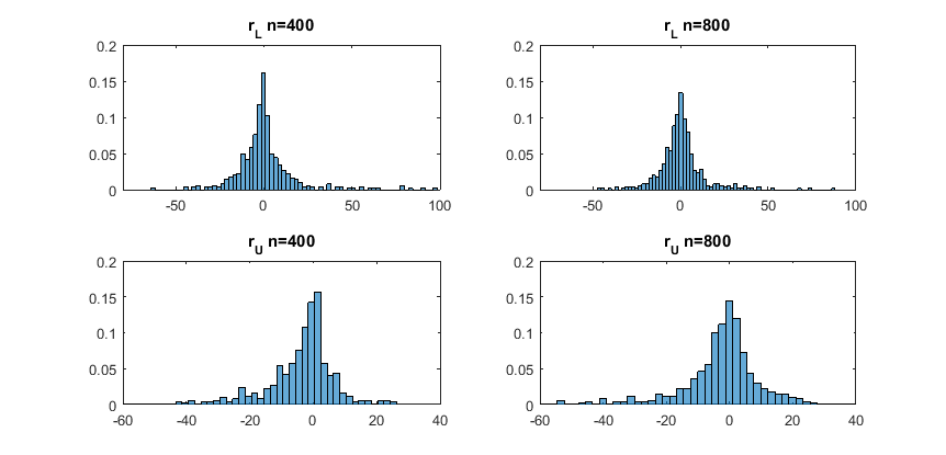
where $\{\varepsilon_{t}\}$ are independently and identically distributed with standard normality. The estimation procedure discussed in Section 3.1 is employed. The range of the boundary parameters $r_{L}$ and $r_{U}$ is set from 10th percentile to 90th percentile of each sample. And the maximum delay parameter $d_{max}$ is set to be 6. For each sample size $n=400,800$, $d$ can be correctly identified for all 500 replications respectively. The bias, the empirical standard deviation (ESD) and the asymptotic standard deviation (ASD) are listed in Table 1. We can observe the bias and the empirical standard deviation decrease as the sample size increases and all the ESDs are close to corresponding ASDs, which are consistent with the asymptotic results in Theorem 2 and Theorem 3. Note the ASD of boundary parameters $r_{L}$ and $r_{U}$ cannot be estimated and only the ESD are included in Table 1. We observe the ESD of $r_{L}$ and $r_{U}$ are approximately reduced by one half when the sample size doubles, which is evidence supporting the super-consistency of boundary parameters. For each sample size, the histograms of $n(\hat{r}_{L}-r_{0L})$ and $n(\hat{r}_{U}-r_{0U})$ are displayed in Figure 1, whose shapes are close to the ones reported in Li et al. (2013) and Li, Guan, Li, and Yu (2015)

We now evaluate the finite sample performance of model selection criteria (BIC) in Section 3.3. The data generating process is the same as (4.1). The sample size is 800, and there are 150 replications. The maximum order $p_{max}$ for each regime’s conditional mean and conditional variance is set to be 6. And the maximum delay parameter $d_{max}$ is still set to be 6. As a result, the BIC correctly identifies all true orders at a rate of 100$\%$.

5 Empirical Analysis

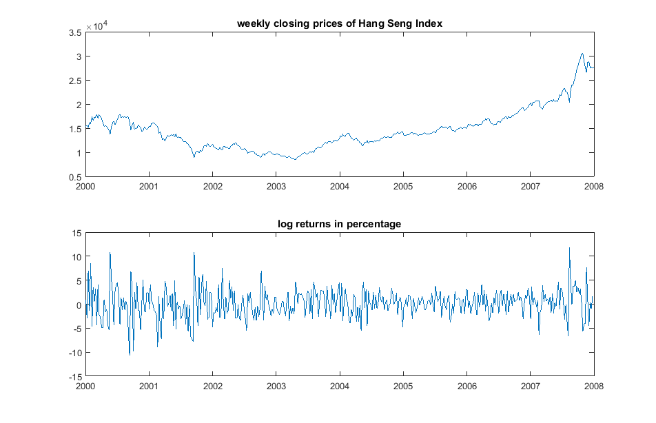
This section considers the weekly closing prices of Hang Seng Index over the period January 2000 to December 2007. We focus on the log return in percentage $y_{t}=100(\log P_{t}-\log P_{t-1})$, where $P_{t}$ is the weekly closing price at time t. There are 417 observations of $\{y_{t}\}$ in total. The plot of $\{P_{t}\}$ and $\{y_{t}\}$ are displayed in Figure 2. Li et al. (2016) have studied this series and they conclude the existence of nonlinearity, ARCH effect and threshold effect through Tsay’s test (Tsay (1986)), Mcleod-Li’s test (Mcleod and Li (1983)) and their score-based test respectively. The two-regime threshold double autoregressive model (TDAR) is employed to fit the data in Li et al. (2016). Since TDAR model can be considered as a special case of BDAR model, it motivates us to consider the proposed BDAR model to fit the percentage log return series.

The range of boundary parameters $r_{L}$ and $r_{U}$ is from the 10th to the 90th empirical percentiles of observations. The maximum delay parameter $d_{max}$ is set to be 6 and the maximum order $p_{max}$ for each regime’s conditional mean and conditional variance is set to be 5. Based on BIC, we have the following fitted model:

$$y_{t}=\left\{\begin{array}[]{lc}0.3937_{0.2621}+0.0385_{0.1318}y_{t-1}+0.2093_{0.0894}y_{t-2}+\varepsilon_{t}\sigma_{t}&\hskip 28.45274ptR_{t}=1\\ -0.5992_{0.2665}+0.2354_{0.0970}y_{t-1}+\varepsilon_{t}\sigma_{t}&\hskip 28.45274ptR_{t}=0\end{array}\right.$$ (5.1)

where

$$\sigma_{t}^{2}=\left\{\begin{array}[]{lc}5.3991_{0.9225}+0.5432_{0.1583}y_{t-1}^{2}+0.1787_{0.1161}y_{t-2}^{2}&\hskip 28.45274ptR_{t}=1\\ 3.4473_{0.7086}+0.0263_{0.0599}y_{t-1}^{2}+0.0678_{0.0578}y_{t-2}^{2}+0.1416_{0.0631}y_{t-3}^{2}&\hskip 28.45274ptR_{t}=0\end{array}\right.$$

with the regime indicator

$$R_{t}=\left\{\begin{array}[]{cl}1&\text{if $y_{t-1}\leq-0.2048$}\\ 0&\text{if $y_{t-1}>0.8770$}\\ R_{t-1}&\text{otherwise}\end{array}\right.$$

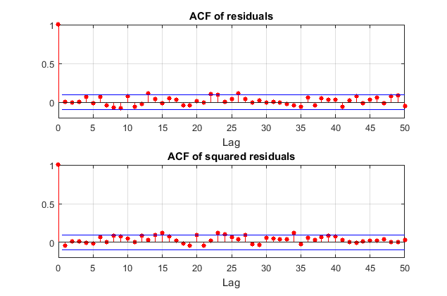
where the subscripts of parameter estimates are their associated standard errors. Figure 3 displays respectively ACFs of residuals and squared residuals, and they slightly go beyond the 95$\%$ confidence bands only at a few lags, which partially suggests the adequacy of the fitted model. To further investigate the fit-adequacy, the Ljung-Box test statistic $Q_{m}$ and the McLeod-Li test statistic $\widetilde{Q}_{m}$ are employed. Generally, m takes value 6 and 12, see Tse (2002) for a discussion on the choice of m. The p-values for of $Q_{6}$, $Q_{12}$, $\widetilde{Q}_{6}$ and $\widetilde{Q}_{12}$ are 0.6590, 0.3666, 0.8200 and 0.4013 respectively, which further suggests the fit-adequacy at 5$\%$ significance level.

The asymmetry of the buffered zone around 0 might be interpreted as market participants are more sensitive to losses and gains. Based on the fitted model, the investors require the return of previous week to go above 0.8770$\%$ to confirm a good time, approximately three times larger in absolute value than the signal of a bad time. When the previous week’s return lies in the buffer zone [-0.2048$\%$ 0.8770$\%$], investors are not sure about the market condition, so they trace back to learn $R_{t-1}$, which may depend on returns several periods ago. Therefore, the buffered double autoregressive model will further rely on the information contained in the dynamic momentum structure, when the past week’s return alone is not quite informative on the market conditions. The BDAR model provides a more realistic characterization on the regime switching mechanism than the traditional two-regime threshold type model. The sudden switch of the probabilistic structure as in the traditional threshold time series models can be delayed by the incorporation of the buffer zone.

Another feature of the fitted BDAR model is the asymmetry of volatility. The coefficients in the lower regime’s conditional variance is much larger than their counterparts in the upper regime. This asymmetry can be interpenetrated as the stock market is more volatile during bad times.

6 Appendix

6.1 Proof of Theorem 1

As in the main part of the paper, define

$$Y_{t}=\begin{bmatrix}y_{t}\\ y_{t-1}\\ \vdots\\ y_{t-p+1}\\ R_{t}\\ \end{bmatrix}$$

$$M_{0t}=\begin{bmatrix}\phi_{10}I(A_{t})+\phi_{20}I(A_{t}^{c})\\ 0\\ \vdots\\ 0\\ I(y_{t-d}\leqslant r_{L})\\ \end{bmatrix}\quad\quad M_{1t}=\begin{bmatrix}m_{1t}&m_{2t}&\dots&m_{pt}&0\\ 1&0&\dots&0&0\\ \vdots&\vdots&\vdots&\vdots&\vdots\\ \vdots&\vdots&\vdots&\vdots&\vdots\\ 0&0&\dots&\dots&I(r_{L}<y_{t-d}\leqslant r_{U})\\ \end{bmatrix}$$

$g_{1}(Y_{t-1})=M_{0t}+M_{1t}Y_{t-1}$

$$g_{2}(Y_{t-1})=\begin{bmatrix}\sqrt{(\alpha_{10}+\sum_{j=1}^{p}\alpha_{1j}y_{t-j}^{2})I(A_{t})+(\alpha_{20}+\sum_{j=1}^{p}\alpha_{2j}y_{t-j}^{2})I(A_{t}^{c})}\\ 0\\ \vdots\\ 0\\ \end{bmatrix}$$

$Y_{t}=g_{1}(Y_{t-1})+\epsilon_{t}g_{2}(Y_{t-1})\quad\text{ forms a Markov Chain}$

Let $\mathcal{B}^{p}$ be the class of Borel sets of $\mathcal{R}^{p}$, $\mu_{p+1}$ be the Lebesgue measure on $\mathcal{R}^{p+1}$ and $\mathcal{U}=\{\emptyset,\{0\},\{1\},\{0,1\}\}$

We denote its state space by $(\mathcal{R}^{p}\times\{0,1\},\mathcal{B}^{p}\times\mathcal{U},\mu_{p+1})$ and sets its transition probability function as:

$P(x,A)=\int_{A_{1}}f_{\epsilon}(y)dy,\quad x\in\mathcal{R}^{p}\times\{0,1\}\text{ and }A\in\mathcal{B}^{p}\times\mathcal{U}$

Where $A_{1}=\{\epsilon:\epsilon g_{2}(x)+g_{1}(x)\in A\}$ and $f_{\epsilon}(\cdot)$ is the density of $\epsilon_{t}$.

By a method similar to Lemma 1 and 2 of Lu (1998), it can be shown that the chain is $\mu_{p+1}$-irreducible and aperiodic, and non-null compact sets are small sets.

Before we proceed, we need to state one lemma and one theorem. The lemma is proved in Lee (2006) and the theorem comes from Tweedie (1983):

Lemma 6.1.

(Lemma 2.2 in Lee (2006)) Let $V(z)=\sum_{i=1}^{n}\gamma_{i}|z_{i}|^{r},z=(z_{1},z_{2},\dots,z_{n}),n\in Z^{+},r>0$. If $\sum_{i=1}^{n}\xi_{i}<1$ with $\xi_{i}\geqslant 0$, we may choose $\gamma_{i}>0,i=1,\dots,n$ so that for some positive constant $\rho<1,\gamma_{1}(\sum_{i=1}^{n}\xi_{i}|z_{i}|^{r})+\sum_{i=2}^{n}\gamma_{i}|z_{i-1}|^{r}\leqslant\rho V(z)$.

Theorem 6.2.

(Theorem 4 in Tweedie (1983)) Suppose that the Markov process $\{Y_{t}:t\geqslant 0\}$ is aperiodic $\mu$-irreducible and $\mathcal{B}$ is a small set. Suppose there are constants $\rho<1,\epsilon>0$ and a measurable function $V\geqslant 1$ such that

$E[V(Y_{t})|Y_{t-1}=z]\leqslant\rho V(z)-\epsilon,z\in\mathcal{B}^{c}$

$\sup_{z\in\mathcal{B}}E[V(Y_{t})|Y_{t-1}=z]<\infty$

then the Markov process $Y_{t}$ is geometrically ergodic.

We continue the proof. Let $b_{j}=\underset{1\leqslant i\leqslant 2}{max}|\phi_{ij}|,0\leqslant j\leqslant p,\quad a_{j}=\underset{1\leqslant i\leqslant 2}{max}\alpha_{ij},0\leqslant j\leqslant p$. Define a test function $V$ by:

$V(Y_{t})=\sum\limits_{i=1}^{p}\gamma_{i}|y_{t+1-i}|^{r}+1$

$|y_{t}|\leqslant b_{0}+\sum\limits_{j=1}^{p}b_{j}|y_{t-j}|+|\epsilon_{t}|(a_{0}+\sum\limits_{j=1}^{p}a_{j}y_{t-j}^{2})^{\frac{1}{2}}$

Define:

$$s_{1}(y_{t-1},\dots,y_{t-p})=b_{0}+\sum\limits_{j=1}^{p}|y_{t-j}|b_{j}$$

$$s_{2}(y_{t-1},\dots,y_{t-p})=[a_{0}+\sum\limits_{j=1}^{p}y_{t-j}^{2}a_{j}]^{\frac{1}{2}}$$

Similar to Lee (2006), we have:

$$s_{1}^{r}\leqslant\left\{\begin{aligned} &b_{0}^{r}+\sum\limits_{j=1}^{p}b_{j}^{r}|y_{t-j}|^{r},&&0<r\leqslant 1\\ &(1+\epsilon)^{r}(\sum\limits_{j=1}^{p}b_{j})^{r-1}(\sum\limits_{j=1}^{p}b_{j}|y_{t-j}|^{r}),&&1<r\leqslant 2,\forall\epsilon>0,\exists M(\epsilon)s.t.||Y_{t-1}||>M(\epsilon)\\ \end{aligned}\right.$$

$$s_{2}^{r}\leqslant a_{o}^{\frac{r}{2}}+\sum\limits_{j=1}^{p}a_{j}^{\frac{r}{2}}|y_{t-j}|^{r},\quad 0<r\leqslant 2$$

Moreover, when $0<r\leqslant 1$, by basic inequality, we have $E[|y_{t}|^{r}|Y_{t-1}]\leqslant s_{1}^{r}+s_{2}^{r}E|\epsilon_{t}|^{r}$

When $1<r\leqslant 2$, note $\epsilon_{t}$ is symmetric by assumption, by the following inequality:

$$(1+x)^{r}+(1-x)^{r}\leqslant 2(|x|^{r}+1),-1\leq x\leq 1$$

we can show that

$$E[|s_{1}+s_{2}\epsilon_{t}|^{r}|Y_{t-1}]=\frac{1}{2}E[|s_{1}+s_{2}\epsilon_{t}|^{r}+|s_{1}-s_{2}\epsilon_{t}|^{r}|Y_{t-1}]\leqslant s_{1}^{r}+s_{2}^{r}E|\epsilon_{t}|^{r}$$

$\begin{aligned} \text{Therefore, }&E[V(Y_{t})|Y_{t-1}]\\ &\leqslant\gamma_{1}(s_{1}^{r}+s_{2}^{r}E|\epsilon_{t}|^{r})+\sum\limits_{i=2}^{p}\gamma_{i}|y_{t+1-i}|^{r}+1\\ &\leqslant\gamma_{1}\sum\limits_{i=1}^{p}\xi_{i}|y_{t-i}|^{r}+\sum\limits_{i=2}^{p}\gamma_{i}|y_{t+1-i}|^{r}+1+C_{1},\\ &\quad\text{ where }C_{j}\text{ is a generic notation for positive constants}\\ \end{aligned}$
 

$\sum\limits_{i=1}^{p}\xi_{i}=\left\{\begin{aligned} &\sum\limits_{j=1}^{p}b_{j}^{r}+\sum\limits_{j=1}^{p}a_{j}^{\frac{r}{2}}E|\epsilon_{t}|^{r},&&0<r\leqslant 1\\ &(1+\epsilon)^{r}(\sum\limits_{j=1}^{p}b_{j})^{r}+\sum\limits_{j=1}^{p}a_{j}^{\frac{r}{2}}E|\epsilon_{t}|^{r},&&1<r\leqslant 2,\forall\epsilon>0,\exists M(\epsilon),s.t.||Y_{t-1}||>M(\epsilon)\\ \end{aligned}\right.$
 

By Lemma 6.1, we can set $\sum\limits_{i=1}^{p}\xi_{i}<1$ and find $\gamma_{i}>0,i=1,\dots,p$ such that for $||z||>M,\exists$ some constants $\rho<1,E[V(Y_{t})|Y_{t-1}=z]\leqslant\rho V(z)+C_{2}$. Thus, inequalities in Theorem 6.2 hold with some $\epsilon>0$ and compact set $\mathcal{B}=\{||z||\leqslant M\}$ for sufficiently large $M<\infty$, since $V(z)$ increases as $||z||$ increases. Hence, we obtain the geometric ergodicity and hence the strict stationarity.

To prove the third part of the theorem, define $V(z)=\sum\limits_{i=1}^{p}\gamma_{i}z_{i}^{4}+1$ from $E(\epsilon_{t})=E(\epsilon_{t}^{3})=0$ for $||z||>M$.

$\begin{aligned} &E[(s_{1}+s_{2}\epsilon_{t})^{4}|Y_{t-1}]\leqslant[(1+3E(\epsilon_{t}^{2}))s_{1}^{4}+(E\epsilon_{t}^{4}+3E\epsilon_{t}^{2})s_{2}^{4}]\\ &s_{1}^{4}\leqslant(1+\epsilon)^{4}(\sum\limits_{j=1}^{p}b_{j}y_{t-j}^{4})(\sum\limits_{j=1}^{p}b_{j})^{3}\\ &s_{2}^{4}\leqslant(1+\epsilon)^{2}(\sum\limits_{j=1}^{p}a_{j}y_{t-j}^{4})(\sum\limits_{j=1}^{p}a_{j})\\ \end{aligned}$

Therefore for $||z||>M$

$\begin{aligned} E[V(Y_{t})|Y_{t-1}=z]&\leqslant\gamma_{1}\{[1+3E(\epsilon_{t}^{2})]s_{1}^{4}+[E(\epsilon_{t}^{4})+3E(\epsilon_{t}^{2})]s_{2}^{4}\}+\sum\limits_{i=2}^{p}\gamma_{i}|y_{t+1-i}|^{4}+1\\ &\leqslant\gamma_{1}\sum\limits_{i=1}^{p}\xi_{i}|y_{t-i}|^{4}+\sum\limits_{i=2}^{p}\gamma_{i}|y_{t+1-i}|^{4}+1\\ \end{aligned}$

where $\sum\limits_{i=1}^{p}\xi_{i}=[1+3E(\epsilon_{t}^{2})](1+\epsilon)^{4}(\sum\limits_{j=1}^{p}b_{j})^{4}+[E(\epsilon_{t}^{4})+3E(\epsilon_{t}^{2})](1+\epsilon)^{2}(\sum\limits_{j=1}^{p}a_{j})^{2}$
By Lemma 6.1, we can set $\sum\limits_{i=1}^{p}\xi_{i}<1$ and obtain the geometric ergodicity as we do in proving the first two parts of the theorem.

6.2 Proof of Theorem 2

Before we prove Theorem 2, we introduce some notations and a preliminary result.

Denote the parameter space as $\Theta=\land\times[a,b]\times[a,b]\times D$, where $\land=\land_{1}\times\land_{2}$.
Parametre vector $\theta=(\phi_{1}^{\prime},\alpha_{1}^{\prime},\phi_{2}^{\prime},\alpha_{2}^{\prime},r_{L},r_{U},d)^{\prime}=(\lambda_{1}^{\prime},\lambda_{2}^{\prime},r_{L},r_{U},d)^{\prime}$, where

$$\mbox{\boldmath{$\lambda_{1}$}}=\begin{bmatrix}\mbox{\boldmath{$\phi_{1}$}}\\ \mbox{\boldmath{$\alpha_{1}$}}\\ \end{bmatrix}\quad\quad\mbox{\boldmath{$\lambda_{2}$}}=\begin{bmatrix}\mbox{\boldmath{$\phi_{2}$}}\\ \mbox{\boldmath{$\alpha_{2}$}}\\ \end{bmatrix}$$

Recall in the main body of the paper, we define
$\begin{aligned} \mbox{\boldmath{$l_{t}(\theta)$}}&=\log{\mbox{\boldmath{$h_{t}$}}(\theta)}+\frac{\mbox{\boldmath{$u_{t}^{2}(\theta)$}}}{\mbox{\boldmath{$h_{t}(\theta)$}}}\\ &=R_{t}\{\log\mbox{\boldmath{$h_{1t}(\theta)$}}+\frac{[y_{t}-\mbox{\boldmath{$\mu_{1t}(\theta)]$}}^{2}}{\mbox{\boldmath{$h_{1t}(\theta)$}}}\}+(1-R_{t})\{{\log\mbox{\boldmath{$h_{2t}(\theta)$}}+\frac{[y_{t}-\mbox{\boldmath{$\mu_{2t}(\theta)]$}}^{2}}{\mbox{\boldmath{$h_{2t}(\theta)$}}}}\}\\ \end{aligned}$  

where for i=1,2

$\begin{aligned} \mbox{\boldmath{$\mu_{it}(\theta)$}}&=\phi_{i0}+\phi_{i1}y_{t-1}+\dots+\phi_{ip}y_{t-p}\\ \mbox{\boldmath{$h_{it}(\theta)$}}&=\alpha_{i0}+\alpha_{i1}y_{t-1}^{2}+\dots+\alpha_{ip}y_{t-p}^{2}\\ \end{aligned}$

We further denote it as $\mbox{\boldmath{$l_{t}(\theta)$}}=R_{t}\mbox{\boldmath{$l_{1t}(\theta)$}}+(1-R_{t})\mbox{\boldmath{$l_{2t}(\theta)$}}$, with

$\begin{aligned} \mbox{\boldmath{$l_{1t}(\theta)$}}&=\log\mbox{\boldmath{$h_{1t}(\theta)$}}+\frac{[y_{t}-\mbox{\boldmath{$\mu_{1t}(\theta)]$}}^{2}}{\mbox{\boldmath{$h_{1t}(\theta)$}}}\\ \mbox{\boldmath{$l_{2t}(\theta)$}}&={\log\mbox{\boldmath{$h_{2t}(\theta)$}}+\frac{[y_{t}-\mbox{\boldmath{$\mu_{2t}(\theta)]$}}^{2}}{\mbox{\boldmath{$h_{2t}(\theta)$}}}}\\ \end{aligned}$

If Assumption 2 and conditions in Theorem 2 hold, Lemma B.2 in Ling (2007) implies that

$$E[\underset{\theta\in\Theta}{\sup}|\mbox{\boldmath{$l_{it}(\theta)$}}|]<\infty\quad\text{i=1,2 and}\quad E[\underset{\theta\in\Theta}{\sup}|\mbox{\boldmath{$l_{t}(\theta)$}}|]<\infty\\$$ (6.3)

This preliminary result will be used to invoke dominance convergence theorem in the following. We are ready to prove Theorem 2 now.

Proof of Theorem 2

Following the method in Huber(1967), it is sufficient for us to verify the following three claims:

• $S1$: $\underset{\theta\in\Theta}{\sup}\frac{1}{n}|\mbox{\boldmath{$\tilde{L}_{n}(\theta)-L_{n}(\theta)$}}|\xrightarrow{a.s.}0$, where $\tilde{L}_{n}(\theta)$ is the modified likelihood function defined in the paper.
  

• $S2$: $E[\mbox{\boldmath{$l_{t}(\theta)$}}]$ is uniquely minimized at $\theta=\theta_{0}=(\phi_{10}^{\prime},\alpha_{10}^{\prime},\phi_{20}^{\prime},\alpha_{20}^{\prime},r_{0L},r_{0U},d_{0})^{\prime}$
  

• $S3$: $E[\underset{\mbox{\boldmath{$\theta^{*}$}}\in U_{\eta}(\mbox{\boldmath{$\theta$}})}{\sup}|\mbox{\boldmath{$l_{t}(\theta)-l_{t}(\theta^{*})$}}|]\xrightarrow{a.s.}0$ as $\eta\to 0$, where $U_{\eta}(\mbox{\boldmath{$\theta$}})=\{\mbox{\boldmath{$\theta^{*}\in\Theta,||\theta^{*}-\theta||$}}<\eta\}$
  
  

Let us first show S1:

$\begin{aligned} \frac{1}{n}|\mbox{\boldmath{$\tilde{L}_{n}(\theta)-L_{n}(\theta)$}}|&=\frac{1}{n}|\sum\limits_{t=1}^{k_{n}}(\mbox{\boldmath{$\tilde{l}_{t}(\theta)-l_{t}(\theta)$}})|\\ &=\{(1-R_{1})\prod\limits_{t=1}^{k_{n}}1(r_{L}<y_{t-d}\leqslant r_{U})\}\{\frac{1}{n}\sum\limits_{t=1}^{k_{n}}[\mbox{\boldmath{$l_{1t}(\theta)-l_{2t}(\theta)$}}]\}\\ &\leqslant\prod\limits_{t=1}^{k_{n}}1(a\leqslant y_{t-d}\leqslant b)\{\frac{1}{n}\sum\limits_{t=1}^{k_{n}}[\mbox{\boldmath{$l_{1t}(\theta)-l_{2t}(\theta)$}}]\}\\ \end{aligned}$

If $\frac{k_{n}}{n}\to 0$, then clearly $\underset{\tiny{\mbox{\boldmath{$\theta\in\Theta$}}}}{\sup}\frac{1}{n}|\mbox{\boldmath{$\tilde{L}_{n}(\theta)-L_{n}(\theta)$}}|\to 0$

If $\frac{k_{n}}{n}\to$ a positive number (constant), then by ergodic theorem, Assumption 1 in the paper and (6.3), we have:

$\underset{\theta\in\Theta}{\sup}\frac{1}{k_{n}}\sum\limits_{t=1}^{k_{n}}[\mbox{\boldmath{$l_{1t}(\theta)-l_{2t}(\theta)$}}]\xrightarrow{a.s.}E[\underset{\theta\in\Theta}{\sup}[\mbox{\boldmath{$l_{1t}(\theta)-l_{2t}(\theta)$}}]\leqslant E[\underset{\theta\in\Theta}{\sup}[\mbox{\boldmath{$l_{1t}(\theta)$}}]+E[\underset{\theta\in\Theta}{\sup}\mbox{\boldmath{$l_{2t}(\theta)$}}]<\infty$

Moreover, by Assumption 1,

$\frac{1}{k_{n}}\sum\limits_{t=1}^{k_{n}}1(y_{t-d}<a\text{ or }y_{t-d}>b)\to Pr(y_{t-d}<a\text{ or }y_{t-d}>b)>0$

$Pr(\underset{k_{n}\to\infty}{\lim}\prod\limits_{t=1}^{k_{n}}1(a\leqslant y_{t-d}\leqslant b)=1)=Pr(\underset{k_{n}\to\infty}{\lim}\frac{1}{k_{n}}\sum\limits_{t=1}^{k_{n}}1(y_{t-d}<a\text{ or }y_{t-d}>b)=0)=0$

$i.e.,\underset{k_{n}\to\infty}{\lim}\prod\limits_{t=1}^{k_{n}}1(a\leqslant y_{t-d}\leqslant b)\to 0$ as $k_{n}\to\infty$.

Therefore, we still have $\underset{\tiny{\mbox{\boldmath{$\theta\in\Theta$}}}}{\sup}\frac{1}{n}|\mbox{\boldmath{$\tilde{L}_{n}(\theta)-L_{n}(\theta)$}}|\to 0$. We finish the proof of $S1$.

Let us then show $S2$:

$\begin{aligned} &E_{\theta_{0}}\{\mbox{\boldmath{$l_{t}(\theta)$}}\}-E_{\theta_{0}}\{\mbox{\boldmath{$l_{t}(\theta_{0})$}}\}\\ &=E_{\theta_{0}}\{[\mbox{\boldmath{$l_{1t}(\theta)-l_{1t}(\theta_{0})$}}]R_{0t}R_{t}\}+E_{\theta_{0}}\{[\mbox{\boldmath{$l_{2t}(\theta)-l_{2t}(\theta_{0})$}}](1-R_{0t})(1-R_{t})\}\\ &+E_{\theta_{0}}\{[\mbox{\boldmath{$l_{1t}(\theta)-l_{2t}(\theta_{0})$}}](1-R_{0t})R_{t}\}+E_{\theta_{0}}\{[\mbox{\boldmath{$l_{2t}(\theta)-l_{1t}(\theta_{0})$}}]R_{0t}(1-R_{t})\}\\ \end{aligned}$

$\begin{aligned} \text{Consider }&E_{\theta_{0}}[(\mbox{\boldmath{$l_{1t}(\theta)-l_{2t}(\theta_{0}))$}}R_{0t}R_{t}]\\ &=E_{\theta_{0}}\{(\log\frac{\mbox{\boldmath{$\alpha_{1}^{\prime}X_{t-1}$}}}{\mbox{\boldmath{$\alpha_{10}^{\prime}X_{t-1}$}}}+\frac{\mbox{\boldmath{$\alpha_{10}^{\prime}X_{t-1}$}}}{\mbox{\boldmath{$\alpha_{1}^{\prime}X_{t-1}$}}}-1+\frac{[(\mbox{\boldmath{$\phi_{10}-\phi_{1})^{\prime}Y_{t-1}$}}]^{2}}{\mbox{\boldmath{$\alpha_{1}^{\prime}X_{t-1}$}}})R_{0t}R_{t}\}\\ \end{aligned}$

By $\log\frac{1}{x}+x-1\geqslant 0$, we know:

$E_{\theta_{0}}\{[\mbox{\boldmath{$l_{1t}(\theta)-l_{2t}(\theta)$}}]R_{0t}R_{t}\}\geqslant 0$ with equality iff $\frac{\mbox{\boldmath{$\alpha_{1}^{\prime}X_{t-1}$}}}{\mbox{\boldmath{$\alpha_{10}^{\prime}X_{t-1}$}}}=1$ and $(\mbox{\boldmath{$\phi_{10}-\phi_{1})^{\prime}Y_{t-1}$}}=0,i.e.,\mbox{\boldmath{$\alpha_{1}=\alpha_{10}$}},\mbox{\boldmath{$\phi_{1}=\phi_{10}$}}$

Similarly, we have:

$E_{\theta_{0}}\{[\mbox{\boldmath{$l_{2t}(\theta)-l_{2t}(\theta_{0})$}}](1-R_{0t})(1-R_{t})\}\geqslant 0$ with equality iff $\frac{\mbox{\boldmath{$\alpha_{2}^{\prime}X_{t-1}$}}}{\mbox{\boldmath{$\alpha_{20}^{\prime}X_{t-1}$}}}=1$ and $(\mbox{\boldmath{$\phi_{20}-\phi_{2})^{\prime}Y_{t-1}$}}=0,i.e.,\mbox{\boldmath{$\alpha_{2}=\alpha_{20}$}},\mbox{\boldmath{$\phi_{2}=\phi_{20}$}}$

For the third term, we have $E_{\theta_{0}}\{[\mbox{\boldmath{$l_{1t}(\theta)-l_{2t}(\theta_{0})$}}](1-R_{0t})R_{t}\}\geq 0$. Since we assume $\phi_{10}\neq\phi_{20}$ and $\alpha_{10}\neq\alpha_{20}$, $E_{\theta_{0}}\{[\mbox{\boldmath{$l_{1t}(\theta)-l_{2t}(\theta_{0})$}}](1-R_{0t})R_{t}\}=0$ implies $E_{\theta_{0}}\{(1-R_{0t})R_{t}\}=0$, from which it can be deduced, following the same argument in proving Theorem 2 in Li, Guan, Li, and Yu (2015), that $d=d_{0},r_{L}\geqslant r_{0L},r_{U}\geqslant r_{0U}$. Similarly, from the last term $E_{\theta_{0}}\{[\mbox{\boldmath{$l_{2t}(\theta)-l_{1t}(\theta_{0})$}}]R_{0t}(1-R_{t})\}=0$, we have $d=d_{0},r_{L}\leqslant r_{0L},r_{U}\leqslant r_{0U}$. We thus finish the proof of $S2$.

Let us further show $S3$:

$\mbox{\boldmath{$\theta$}}^{*}\in U_{\eta}(\mbox{\boldmath{$\theta$}})$

$$\mbox{\boldmath{$l_{t}(\theta^{*})-l_{t}(\theta)$}} =\{\mbox{\boldmath{$l_{1t}(\theta^{*})-l_{1t}(\theta)$}}\}R_{t}(r_{L}^{*},r_{U}^{*},d)$$ (6.4)

$$+\mbox{\boldmath{$l_{1t}(\theta)$}}[R_{t}(r_{L}^{*},r_{U}^{*},d)-R_{t}(r_{L},r_{U},d)]$$

$$+[\mbox{\boldmath{$l_{2t}(\theta^{*})-l_{2t}(\theta)$}}][1-R_{t}(r_{L}^{*},r_{U}^{*},d)]$$

$$+\mbox{\boldmath{$l_{2t}(\theta)$}}[R_{t}(r_{L},r_{U},d)-R_{t}(r_{L}^{*},r_{U}^{*},d)]$$

$$\mbox{\boldmath{$l_{1t}(\theta^{*})-l_{1t}(\theta)$}} =\log{\mbox{\boldmath{$\alpha_{1}^{*}$}}^{\prime}X_{t-1}}-\log\mbox{\boldmath{$\alpha_{1}^{\prime}X_{t-1}$}}$$

$$+\frac{(y_{t}-\mbox{\boldmath{${\phi_{1}^{*}}^{\prime}Y_{t-1}$}})^{2}-(y_{t}-\mbox{\boldmath{${\phi_{1}^{\prime}Y_{t-1}})^{2}$}}}{\mbox{\boldmath{${\alpha_{1}^{*}}^{\prime}X_{t-1}$}}}$$

$$+(y_{t}-\mbox{\boldmath{${\phi_{1}^{\prime}Y_{t-1}}$}})^{2}[\frac{1}{\mbox{\boldmath{${\alpha_{1}^{*}}^{\prime}X_{t-1}$}}}-\frac{1}{\mbox{\boldmath{$\alpha_{1}^{\prime}X_{t-1}$}}}]$$

By Taylor’s expansion and a method similar to Zhu and Ling (2013), we have:

$\begin{aligned} &E[\underset{\theta^{*}\in U_{\eta}(\theta)}{\sup}|\log{\mbox{\boldmath{$\alpha_{1}^{*}$}}^{\prime}X_{t-1}}-\log{\mbox{\boldmath{$\alpha_{1}$}}^{\prime}X_{t-1}}|]\to 0\quad\text{as}\quad\eta\to 0\\ &E[\underset{\theta^{*}\in U_{\eta}(\theta)}{\sup}|\frac{(y_{t}-\mbox{\boldmath{${\phi_{1}^{*}}^{\prime}Y_{t-1}$}})^{2}-(y_{t}-\mbox{\boldmath{${\phi_{1}}^{\prime}Y_{t-1}$}})^{2}}{\mbox{\boldmath{${\alpha_{1}^{*}}^{\prime}X_{t-1}$}}}|]\to 0\quad\text{as}\quad\eta\to 0\\ &E[\underset{\theta^{*}\in U_{\eta}(\theta)}{\sup}|(y_{t}-\mbox{\boldmath{${\phi_{1}^{\prime}Y_{t-1}}$}})^{2}(\frac{1}{\mbox{\boldmath{${\alpha_{1}^{*}}^{\prime}X_{t-1}$}}}-\frac{1}{\mbox{\boldmath{$\alpha_{1}^{\prime}X_{t-1}$}}})|]\to 0\quad\text{as}\quad\eta\to 0\\ \end{aligned}$

Therefore, the first and third terms in expression (6.4) can be dealt with.

We now look at the second term in (6.4).

Since $l_{1t}(\theta)$ and $R_{t}(r_{L}^{*},r_{U}^{*},d)-R_{t}(r_{L},r_{U},d)$ have non-overlapping parameters,

$E\{\underset{\theta^{*}\in U_{\eta}(\theta)}{\sup}\mbox{\boldmath{$l_{1t}(\theta)$}}[R_{t}(r_{L}^{*},r_{U}^{*},d)-R_{t}(r_{L},r_{U},d)]\}=E\{\underset{\theta^{*}\in U_{\eta}(\theta)}{\sup}\mbox{\boldmath{$l_{1t}(\theta)$}}\underset{\theta^{*}\in U_{\eta}(\theta)}{\sup}[R_{t}(r_{L}^{*},r_{U}^{*},d)-R_{t}(r_{L},r_{U},d)]\}$

Li, Guan, Li, and Yu (2015) shows that $E\{\underset{\theta^{*}\in U_{\eta}(\theta)}{\sup}|R_{t}(r_{L}^{*},r_{U}^{*},d)-R_{t}(r_{L},r_{U},d)|\}\to 0\quad\text{as}\quad\eta\to 0$. Combining this with $E[\underset{\theta^{*}\in U_{\eta}(\theta)}{\sup}|\mbox{\boldmath{$l_{1t}(\theta)$}}|]<\infty$ and using dominated convergence theorem, we have:

$E\{\underset{\theta^{*}\in U_{\eta}(\theta)}{\sup}\mbox{\boldmath{$l_{1t}(\theta)$}}[R_{t}(r_{t}^{*},r_{U}^{*},d)-R_{t}(r_{t},r_{U},d)]\}\to 0$ as $\eta\to 0$

The fourth term in (6.4) can be dealt with in the same way. We thus finish the proof of $S3$.

Based on $S1$-$S3$ and Huber (1967), Theorem 2 is proved.

6.3 Proof of Theorem 3

We first prove the super-consistency of the estimated boundary parameters at Claim (i). Note in Theorem 2, we know $\hat{\theta}_{n}$ is strong consistent. Therefore, without loss of generality, we restrict the parameter space to a neighborhood of $\theta_{0}$.

Define $w(\triangle)=\{\mbox{\boldmath{$\lambda$}}\in\mbox{\boldmath{$\land$}},a<r_{L}<r_{U}<b:||\mbox{\boldmath{$\lambda-\lambda_{0}$}}||<\triangle,|r_{L}-r_{0L}|<\triangle,|r_{U}-r_{0U}|<\triangle\},$ where $0<\triangle<\min\{1,\frac{r_{0U}-r_{0L}}{2}\}$ will be determined later. As in Chan (1993), it is sufficient to show for any $\epsilon>0,\exists$ a positive $K$ such that:

$$\text{Pr}(\tilde{L}_{n}(\mbox{\boldmath{$\lambda$}},r_{0L}+z_{L},r_{0U}+z_{U})-\tilde{L}_{n}(\mbox{\boldmath{$\lambda$}},r_{0L},r_{0U})>0)>1-\epsilon$$ (6.5)

where $\mbox{\boldmath{$\lambda$}}\in w(\triangle),|z_{L}|>\frac{K}{n},|z_{U}|>\frac{K}{n}$.

We consider the case $p=d=1$,$z_{L}<0$ and $z_{U}>0$. Denote the disjoint events:

$\begin{aligned} &A_{0}=\{r_{0U}<y_{t-1}\leqslant r_{0U}+z_{U},R_{t-1}=1\}\\ &B_{0}=\{r_{0L}+z_{L}<y_{t-1}\leqslant r_{0L},R_{t-1}=0\}\\ &A_{i}=\{y_{t-1}\in(r_{0L},r_{0U}],\dots,y_{t-i}\in(r_{0L},r_{0U}],r_{0U}<y_{t-i-1}\leqslant r_{0U}+z_{U},R_{t-i-1}=1\},i\geqslant 1\\ &B_{i}=\{y_{t-1}\in(r_{0L},r_{0U}],\dots,y_{t-i}\in(r_{0L},r_{0U}],r_{0L}+z_{L}<y_{t-i-1}\leqslant r_{0L},R_{t-i-1}=0\},i\geqslant 1\\ \end{aligned}$

where $R_{t}\equiv R_{t}(r_{0L}+z_{L},r_{0U}+z_{U})$. Denote $A_{t}(z_{L},z_{U})=\bigcup\limits_{j=0}^{\infty}A_{j},B_{t}(z_{L},z_{U})=\bigcup\limits_{j=0}^{\infty}B_{j}$
As in Li, Guan, Li, and Yu (2015), we have:

$R_{t}(r_{0L}+z_{L},r_{0U}+z_{U})-R_{t}(r_{0L},r_{0U})=1\{A_{t}(z_{L},z_{U})\}-1\{B_{t}(z_{L},z_{U})\}$

Moreover, $B_{t}(z_{L},z_{U})\subset\{R_{t}(r_{0L},r_{0U})=1\},A_{t}(z_{L},z_{U})\subset\{R_{t}(r_{0L},r_{0U})=0\}$. As a result,

$\begin{aligned} &\mbox{\boldmath{$L_{n}(\lambda$}},r_{0L}+z_{L},r_{0U}+z_{U})-\mbox{\boldmath{$L_{n}(\lambda$}},r_{0L},r_{0U})\\ &=\sum\limits_{t=1}^{n}\mbox{\boldmath{$(l_{1t}(\theta)-l_{2t}(\theta))$}}[1\{A_{t}(z_{L},z_{U})\}-1\{B_{t}(z_{L},z_{U})\}]\\ &=\sum\limits_{t=1}^{n}\mbox{\boldmath{$(l_{1t}(\theta)-l_{2t}(\theta))$}}1\{A_{t}(z_{L},z_{U})\}+\sum\limits_{t=1}^{n}\mbox{\boldmath{$(l_{2t}(\theta)-l_{1t}(\theta))$}}1\{B_{t}(z_{L},z_{U})\}\\ &=\mbox{\boldmath{$L_{1n}$}}(z_{L},z_{U})+\mbox{\boldmath{$L_{2n}$}}(z_{L},z_{U})\\ \end{aligned}$

Our next step is to show that

$$\qquad\qquad\qquad\qquad\text{Pr}(\mbox{\boldmath{$L_{1n}$}}(z_{L},z_{U})>0)>1-\epsilon$$ (6.6)

when $\mbox{\boldmath{$\lambda$}}\in w(\triangle),-\triangle<z_{L}<0,\frac{K}{n}<z_{U}<\triangle$.

$\begin{aligned} \text{Define }&Q_{z_{L}}(z_{U})=E[1\{A_{t}(z_{L},z_{U})\}]\\ &Q_{n,z_{L}}(z_{U})=\frac{1}{n}\sum\limits_{t=1}^{n}1\{A_{t}(z_{L},z_{U})\}\\ \end{aligned}$

By a calculation, we can obtain

$\begin{aligned} &\frac{\mbox{\boldmath{$L_{1n}$}}(z_{L},z_{U})}{nQ_{z_{L}}(z_{U})}\equiv\frac{\sum\limits_{t=1}^{n}[\mbox{\boldmath{$l_{1t}(\theta)-l_{2t}(\theta)$}}][1\{A_{t}(z_{L},z_{U})\}]}{nQ_{z_{L}}(z_{U})}\\ &=\frac{\sum\limits_{t=1}^{n}[\log\frac{\mbox{\boldmath{$\alpha_{10}^{\prime}X_{t-1}$}}}{\mbox{\boldmath{$\alpha_{20}^{\prime}X_{t-1}$}}}+\frac{\mbox{\boldmath{$\alpha_{20}^{\prime}X_{t-1}$}}}{\mbox{\boldmath{$\alpha_{10}^{\prime}X_{t-1}$}}}-1+\frac{\{\mbox{\boldmath{$(\phi_{20}-\phi_{10})^{\prime}Y_{t-1}$}}\}^{2}}{\mbox{\boldmath{$\alpha_{10}^{\prime}X_{t-1}$}}}]1\{A_{t}(z_{L},z_{U})\}}{nQ_{n,z_{L}}(z_{U})}\\ &+\frac{\sum\limits_{t=1}^{n}\frac{2\mbox{\boldmath{$(\phi_{20}-\phi_{10})^{\prime}Y_{t-1}$}}\sqrt{\mbox{\boldmath{$\alpha_{20}^{\prime}X_{t-1}$}}}}{\mbox{\boldmath{$\alpha_{10}^{\prime}X_{t-1}$}}}\epsilon_{t}1\{A_{t}(z_{L},z_{U})\}}{nQ_{n,z_{L}}(z_{U})}\\ &+\frac{\sum\limits_{t=1}^{n}\frac{\mbox{\boldmath{$(\alpha_{20}-\alpha_{10})^{\prime}X_{t-1}$}}}{\mbox{\boldmath{$\alpha_{10}^{\prime}X_{t-1}$}}}(\epsilon_{t}^{2}-1)1\{A_{t}(z_{L},z_{U})\}}{nQ_{n,z_{L}}(z_{U})}+Op(\triangle)\\ \\ \end{aligned}$

Note in the first term,

$\log\frac{\mbox{\boldmath{$\alpha_{10}^{\prime}X_{t-1}$}}}{\mbox{\boldmath{$\alpha_{20}^{\prime}X_{t-1}$}}}+\frac{\mbox{\boldmath{$\alpha_{20}^{\prime}X_{t-1}$}}}{\mbox{\boldmath{$\alpha_{10}^{\prime}X_{t-1}$}}}-1+\frac{\{\mbox{\boldmath{$(\phi_{20}-\phi_{10})^{\prime}Y_{t-1}$}}\}^{2}}{\mbox{\boldmath{$\alpha_{10}^{\prime}X_{t-1}$}}}>0$

where $\mbox{\boldmath{$X_{t-1}$}}=(1,y_{t-1}^{2}),\mbox{\boldmath{$Y_{t-1}$}}=(1,y_{t-1})$

In the second term, $\sum\limits_{t=1}^{n}\frac{2\mbox{\boldmath{$(\phi_{20}-\phi_{10})^{\prime}Y_{t-1}$}}\sqrt{\mbox{\boldmath{$\alpha_{20}^{\prime}X_{t-1}$}}}}{\mbox{\boldmath{$\alpha_{10}^{\prime}X_{t-1}$}}}\epsilon_{t}1\{A_{t}(z_{L},z_{U})\}$ is bounded in absolute value by $K_{1}|\sum\limits_{t=1}^{n}\epsilon_{t}1(A_{t}(z_{L},z_{U}))|$

For the third term, the numerator is bounded in absolute value by $K_{2}|\sum\limits_{t=1}^{n}(\epsilon_{t}^{2}-1)1(A_{t}(z_{L},z_{U}))|$, where $K_{1}$ and $K_{2}$ are some constants independent of $n$.

Following the methond similar to Theorem 3 in Li, Guan, Li, and Yu (2015), we can verify the following three conditions: $\forall\epsilon>0,\eta>0,\exists$ a positive constant $K$ such that as $n$ is large enough,

$Pr[\underset{\frac{k}{n}<z_{U}<\triangle,-\triangle<z_{L}\leqslant 0}{\sup}|\frac{1}{nQ_{zL}(z_{U})}\sum\limits_{t=1}^{n}1\{A_{t}(z_{L},z_{U})\}-1|<\eta]>1-\epsilon$

$Pr[\underset{\frac{k}{n}<z_{U}<\triangle,-\triangle<z_{L}\leqslant 0}{\sup}|\frac{1}{nQ_{zL}(z_{U})}\sum\limits_{t=1}^{n}\epsilon_{t}1\{A_{t}(z_{L},z_{U})\}|<\eta]>1-\epsilon$

$Pr[\underset{\frac{k}{n}<z_{U}<\triangle,-\triangle<z_{L}\leqslant 0}{\sup}|\frac{1}{nQ_{zL}(z_{U})}\sum\limits_{t=1}^{n}(\epsilon_{t}^{2}-1)1\{A_{t}(z_{L},z_{U})\}|<\eta]>1-\epsilon$

Therefore, (6.6) is implied. We can further show a similar result for $\mbox{\boldmath{$L_{2n}$}}(z_{L},z_{U})$, and then that for $L_{n}(\mbox{\boldmath{$\lambda$}},r_{0L}+z_{L},r_{0U}+z_{U})-L_{n}(\mbox{\boldmath{$\lambda$}},r_{0L},r_{0U})$. (6.5) is thus proved for the case that $p=d=1$, $z_{L}<0$ and $z_{U}>0$.

The proof for other cases is similar and hence is omitted. The proof of Claim (ii) in this theorem is similar to that of Theorem 2.2 in Li, Ling, and Li (2013) and that of Theorem 3.2 in Li, Ling, and Zakoian (2015), and is also omitted.

6.4 Proof of Theorem 4

From Theorem 3, we know $n(\hat{r}_{L}-r_{0L})=O_{p}(1)$ and $n(\hat{r}_{U}-r_{0U})=O_{p}(1)$. To further characterize their limiting distributions, we consider the limiting behavior of a sequence of normalized profile objective function defined by:

$\mbox{\boldmath{$\tilde{L}_{n}$}}(z)=\mbox{\boldmath{$L_{n}$}}(\mbox{\boldmath{$\tilde{\lambda}$}}_{n}(r_{0}+\frac{z}{n}),r_{0}+\frac{z}{n})-\mbox{\boldmath{$L_{n}$}}(\mbox{\boldmath{$\tilde{\lambda}$}}_{n}(r_{0}),r_{0})$

where $r_{0}=(r_{0L},r_{0U})^{T}$ and $z=(z_{L},z_{U})^{T}$

$\begin{aligned} \text{Denote }\varphi_{n}(z)&=\sum\limits_{t=1}\xi_{1t}\{1-R_{t-1}(r_{0})\}1\{r_{0L}<y_{t-d}\leqslant r_{0L}+\frac{z_{L}}{n}\}1(z_{L}\geqslant 0)\\ &+\sum\limits_{t=1}\xi_{2t}\{1-R_{t-1}(r_{0})\}1\{r_{0L}+\frac{z_{L}}{n}<y_{t-d}\leqslant r_{0L}\}1(z_{L}<0)\\ &+\sum\limits_{t=1}\xi_{1t}R_{t-1}(r_{0})1\{r_{0U}<y_{t-d}\leqslant r_{0U}+\frac{z_{L}}{n}\}1(z_{U}\geqslant 0)\\ &+\sum\limits_{t=1}\xi_{2t}R_{t-1}(r_{0})1\{r_{0U}+\frac{z_{U}}{n}<y_{t-d}\leqslant r_{0U}\}1(z_{U}<0)\\ \\ \text{where }&\xi_{1t}=\sum\limits_{j=0}^{\infty}\zeta_{1,t+j}H_{t+j,j}\\ &\xi_{2t}=\sum\limits_{j=0}^{\infty}\zeta_{2,t+j}H_{t+j,j}\\ &\zeta_{1t}=\log\frac{\mbox{\boldmath{$\alpha_{10}^{\prime}X_{t-1}$}}}{\mbox{\boldmath{$\alpha_{20}^{\prime}X_{t-1}$}}}+\frac{\{(\mbox{\boldmath{$\phi_{10}-\phi_{20}$}})^{\prime}\mbox{\boldmath{$Y_{t-1}$}}-\epsilon_{t}\sqrt{\mbox{\boldmath{$\alpha_{20}^{\prime}X_{t-1}$}}}\}^{2}}{\mbox{\boldmath{$\alpha_{10}^{\prime}X_{t-1}$}}}-\epsilon_{t}^{2}\\ &\zeta_{2t}=\log\frac{\mbox{\boldmath{$\alpha_{20}^{\prime}X_{t-1}$}}}{\mbox{\boldmath{$\alpha_{10}^{\prime}X_{t-1}$}}}+\frac{\{(\mbox{\boldmath{$\phi_{10}-\phi_{20}$}})^{\prime}\mbox{\boldmath{$Y_{t-1}$}}+\epsilon_{t}\sqrt{\mbox{\boldmath{$\alpha_{10}^{\prime}X_{t-1}$}}}\}^{2}}{\mbox{\boldmath{$\alpha_{20}^{\prime}X_{t-1}$}}}-\epsilon_{t}^{2}\\ &H_{t,j}=\prod\limits_{l=1}^{j}1(r_{0L}<y_{t-d+1-l}\leqslant r_{0U})\end{aligned}$

We first prove that, for any $B>0$,

$$\qquad\qquad\underset{||z||\leqslant B}{\sup}|\mbox{\boldmath{$\tilde{L}_{n}$}}(z)-\varphi_{n}(z)|=o_{p}(1)\\$$ (6.7)

It is sufficient to verify the following two conditions:

$$\underset{||z||\leqslant B}{\sup}|\mbox{\boldmath{$\tilde{L}_{n}$}}(z)-\{\mbox{\boldmath{$L_{n}$}}(\mbox{\boldmath{$\lambda_{0}$}},r_{0}+\frac{z}{n})-\mbox{\boldmath{$L_{n}$}}(\mbox{\boldmath{$\lambda_{0}$}},r_{0})\}|=o_{p}(1)\\$$ (6.8)

$$\underset{||z||\leqslant B}{\sup}|\varphi_{n}(z)-\{\mbox{\boldmath{$L_{n}$}}(\mbox{\boldmath{$\theta_{0}$}},r_{0}+\frac{z}{n})-\mbox{\boldmath{$L_{n}$}}(\mbox{\boldmath{$\theta_{0}$}},r_{0})\}|=o_{p}(1)\\$$ (6.9)

By a method similar to similar to the proof of Theorem 4 in Li, Guan, Li, and Yu (2015), we can use Taylor’s expansion and results of Theorem 3 in current paper to show that (6.8) holds. Below we will verify (6.9).

Denote $R_{t}(z)=R_{t}(r_{0}+\frac{z}{n})$ for simplicity. As in Li, Guan, Li, and Yu (2015), we have:

$$R_{t}(z)-R_{t}(0) =\{R_{t-1}(z)-R_{t-1}(0)\}1(r_{0L}<y_{t-d}\leqslant r_{0U})$$

$$+\{1-R_{t-1}(z)\}1(r_{0L}<y_{t-d}\leqslant r_{0L}+\frac{z_{L}}{n})1(z_{L}\geqslant 0)$$

$$-\{1-R_{t-1}(z)\}1(r_{0L}+\frac{z_{L}}{n}<y_{t-d}\leqslant r_{0L})1(z_{L}<0)$$

$$+R_{t-1}(z)1(r_{0U}<y_{t-d}\leqslant r_{0U}+\frac{z_{U}}{n})1(z_{U}\geqslant 0)$$

$$-R_{t-1}(z)1(r_{0U}+\frac{z_{U}}{n}<y_{t-d}\leqslant r_{0U})1(z_{U}<0)$$

$$\text{and then }R_{t}(z)-R_{t}(0) =\sum\limits_{j=0}^{\infty}H_{t,j}\{1-R_{t-1-j}(z)\}1(r_{0L}<y_{t-d-j}\leqslant r_{0L}+\frac{z_{L}}{n})1(z_{L}\geqslant 0)$$ (6.10)

$$-\sum\limits_{j=0}^{\infty}H_{t,j}\{1-R_{t-1-j}(z)\}1(r_{0L}+\frac{z_{L}}{n}<y_{t-d-j}\leqslant r_{0L})1(z_{L}<0)$$

$$+\sum\limits_{j=0}^{\infty}H_{t,j}R_{t-1-j}(z)1(r_{0U}<y_{t-d-j}\leqslant r_{0U}+\frac{z_{U}}{n})1(z_{U}\geqslant 0)$$

$$-\sum\limits_{j=0}^{\infty}H_{t,j}R_{t-1-j}(z)1(r_{0U}+\frac{z_{U}}{n}<y_{t-d-j}\leqslant r_{0U})1(z_{U}<0)$$

where $H_{t,j}=\prod\limits_{l=1}^{j}1(r_{0L}<y_{t-d+1-l}\leqslant r_{0U})$

$\begin{aligned} \text{Denote }\zeta_{t}&=\mbox{\boldmath{$l_{1t}(\theta_{0})-l_{2t}(\theta_{0})$}}\\ &=\log\mbox{\boldmath{$\alpha_{10}^{\prime}X_{t-1}$}}+\frac{(y_{t}-\mbox{\boldmath{$\phi_{10}^{\prime}Y_{t-1}$}})^{2}}{\mbox{\boldmath{$\alpha_{10}^{\prime}X_{t-1}$}}}-\log\mbox{\boldmath{$\alpha_{20}^{\prime}X_{t-1}$}}-\frac{(y_{t}-\mbox{\boldmath{$\phi_{20}^{\prime}Y_{t-1}$}})^{2}}{\mbox{\boldmath{$\alpha_{20}^{\prime}X_{t-1}$}}}\\ \end{aligned}$

and it holds that $\mbox{\boldmath{$L_{n}$}}(\mbox{\boldmath{$\lambda_{0}$}},r_{0}+\frac{z}{n})-\mbox{\boldmath{$L_{n}$}}(\mbox{\boldmath{$\lambda_{0}$}},r_{0})=\sum\limits_{t=1}^{n}\zeta_{t}\{R_{t}(z)-R_{t}(0)\}$.

For the first term of (6.10), i.e., the case with $z_{L}\geqslant 0$, by a method similar to Li, Guan, Li, and Yu (2015), it can be shown that:

$\underset{||z||\leqslant B}{\sup}||\sum\limits_{t=1}^{n}\zeta_{t}\sum\limits_{j=0}^{\infty}H_{t,j}\{R_{t-1-j}(z)-R_{t-1-j}(0)\}1(r_{0L}<y_{t-d-j}\leqslant r_{0L}+\frac{z_{L}}{n})||=o_{p}(1)$

Note $\zeta_{t}=\zeta_{1t}$ when $R_{t}(0)=0$ and $\zeta_{t}=-\zeta_{2t}$ when $R_{t}(0)=1$. Thus, we have

$\begin{aligned} &\sum\limits_{t=1}^{n}\zeta_{t}\sum\limits_{j=0}^{\infty}H_{t,j}\{1-R_{t-1-j}(0)\}1(r_{0L}<y_{t-d-j}\leqslant r_{0L}+\frac{z_{L}}{n})\\ &=\sum\limits_{j=0}^{\infty}\sum\limits_{t=1-j}^{n-j}\zeta_{t+j}H_{t+j,j}\{1-R_{t-1}(0)\}1(r_{0L}<y_{t-d}\leqslant r_{0L}+\frac{z_{L}}{n})\\ &=\sum\limits_{j=0}^{\infty}(\sum\limits_{t=1}^{n}+\sum\limits_{t=1-j}^{0}-\sum\limits_{t=n-j+1}^{n})\zeta_{t+j}H_{t+j,j}\{1-R_{t-1}(0)\}1(r_{0L}<y_{t-d}\leqslant r_{0L}+\frac{z_{L}}{n})\\ &=\sum\limits_{j=0}^{\infty}\sum\limits_{t=1-j}^{n}\zeta_{t+j}H_{t+j,j}\{1-R_{t-1}(0)\}1(r_{0L}<y_{t-d}\leqslant r_{0L}+\frac{z_{L}}{n})+o_{p}(1)\\ &=\sum\limits_{t=1-j}^{n}\xi_{1t}\{1-R_{t-1}(0)\}1(r_{0L}<y_{t-d}\leqslant r_{0L}+\frac{z_{L}}{n})+o_{p}(1)\\ \end{aligned}$
where the $o_{p}(1)$ is uniformly for $||z||\leqslant B$. See also the proof of Theorem 4 in Li, Guan, Li, and Yu (2015) and Lemma 8.2 in Li, Ling, and Li (2013).

Similarly, we can handle the remaining terms in (6.10). Therefore, (6.9) is implied. With (6.8) and (6.9), it is clear that (6.7) holds.

For the space $\mathbb{D(R}^{2})$, we define the skorohod metric as $d(f,g)=\sum\limits_{k=1}^{\infty}2^{-k}\min\{1,d_{k}(f,g)\}$ for $f,g\in\mathbb{D(R}^{2})$, where $d_{k}(f,g)$ is the skorohod metric on $\mathbb{D}([-k,k]\times[-k,k])$, see also Li, Guan, Li, and Yu (2015), Li and Ling (2012) and (16.4) in Billingsley (1999).

By a technique similar that used in the proof of Theorem 3.3 in Li and Ling (2012) and in the proof of Theorem 5 in Li, Ling, and Zhang (2016), together with Theorem 5.5 in Straf (1972), we are able to conclude that $\{\varphi_{n}(z),z\in\mathbb{R}^{2}\}$ converges weakly to $\{\varphi(z),z\in\mathbb{R}^{2}\}$ as $n\to\infty$.

Moreover, (6.7) implies that $d(\tilde{L}_{n}(z),\varphi_{n}(z))\to 0$ in probability as $n\to\infty$. By Theorem 3.1 in Seijo and Sen (2011), it is readily seen that $n(\hat{r}_{L}-r_{0L})\to M_{-}^{(L)}$ and $n(\hat{r}_{U}-r_{0U})\to M_{-}^{(U)}$ in distribution as $n\to\infty$ respectively. The remainder of the proof is similar to that of Theorem 2 in Chan (1993)).

6.5 Proof of Theorem 5

From Theorem 2 and 3, $\hat{r}_{L}$ and $\hat{r}_{U}$ are super-consistent, and $\hat{d}$ is consistent with integer values. Therefore, it can be assumed that the true values of $(r_{L},r_{U},d)$ are known, indicating the true Regime indicators $R_{t}$ are known.

By definition,
$\begin{aligned} \text{BIC}(p)&=\sum\limits_{t=1}^{n}\mbox{\boldmath{$l_{t}(\hat{\theta})$}}+(2p+2)\log n_{1}+(2p+2)\log n_{2}\\ &=\sum\limits_{t=1}^{n}\mbox{\boldmath{$l_{1t}(\hat{\theta})$}}R_{t}+\sum\limits_{t=1}^{n}\mbox{\boldmath{$l_{2t}(\hat{\theta})$}}(1-R_{t})+(2p+2)\log n_{1}+(2p+2)\log n_{2}\\ &=\sum\limits_{t=1}^{n}\mbox{\boldmath{$l_{1t}(\hat{\lambda}_{1})$}}R_{t}+\sum\limits_{t=1}^{n}\mbox{\boldmath{$l_{2t}(\hat{\lambda}_{2})$}}(1-R_{t})+(2p+2)\log n_{1}+(2p+2)\log n_{2}\\ \end{aligned}$
where $\mbox{\boldmath{$l_{1t}(\theta)$}}=\mbox{\boldmath{$l_{1t}(\lambda_{1})$}}$ and $\mbox{\boldmath{$l_{2t}(\theta)$}}=\mbox{\boldmath{$l_{2t}(\lambda_{2})$}}$ are defined at the beginning of the proof of Theorem 2.

We first consider the case $p>p_{0}$. Below we introduce notations $\mbox{\boldmath{$\lambda$}}^{p}$,$\mbox{\boldmath{$\lambda$}}^{p}_{0}$ and $\hat{\mbox{\boldmath{$\lambda$}}}^{p}$ to emphasize their dependence on the order p. Under the situation $p>p_{0}$, the model with order $p$ corresponds to a bigger model, and we have

$\mbox{\boldmath{$l_{1t}$}}(\mbox{\boldmath{$\lambda$}}_{10}^{p})=\mbox{\boldmath{$l_{1t}$}}(\mbox{\boldmath{$\lambda$}}_{10}^{p_{0}}),\mbox{\boldmath{$l_{2t}$}}(\mbox{\boldmath{$\lambda$}}_{20}^{p})=\mbox{\boldmath{$l_{2t}$}}(\mbox{\boldmath{$\lambda$}}_{20}^{p_{0}})$

By an intermediate result in the proof of Theorem 4 in Li et al. (2017), we know

$\begin{aligned} \qquad\qquad&\sum\limits_{t=1}^{n}\mbox{\boldmath{$l_{1t}$}}(\mbox{\boldmath{$\hat{\lambda}$}}_{1}^{p_{0}})R_{t}-\sum\limits_{t=1}^{n}\mbox{\boldmath{$l_{1t}$}}(\mbox{\boldmath{$\lambda$}}_{10}^{p_{0}})R_{t}=O_{p}(1)\\ &\sum\limits_{t=1}^{n}\mbox{\boldmath{$l_{1t}$}}(\mbox{\boldmath{$\hat{\lambda}$}}_{1}^{p})R_{t}-\sum\limits_{t=1}^{n}\mbox{\boldmath{$l_{1t}$}}(\mbox{\boldmath{$\lambda$}}_{10}^{p})R_{t}=O_{p}(1)\\ &\sum\limits_{t=1}^{n}\mbox{\boldmath{$l_{2t}$}}(\mbox{\boldmath{$\hat{\lambda}$}}_{2}^{p_{0}})(1-R_{t})-\sum\limits_{t=1}^{n}\mbox{\boldmath{$l_{2t}$}}(\mbox{\boldmath{$\lambda$}}_{20}^{p_{0}})(1-R_{t})=O_{p}(1)\\ &\sum\limits_{t=1}^{n}\mbox{\boldmath{$l_{2t}$}}(\mbox{\boldmath{$\hat{\lambda}$}}_{2}^{p})(1-R_{t})-\sum\limits_{t=1}^{n}\mbox{\boldmath{$l_{2t}$}}(\mbox{\boldmath{$\lambda$}}_{20}^{p})(1-R_{t})=O_{p}(1)\\ \end{aligned}$
As a result,
$\begin{aligned} \sum\limits_{t=1}^{n}\mbox{\boldmath{$l_{1t}$}}(\mbox{\boldmath{$\hat{\lambda}$}}_{1}^{p})R_{t}-\sum\limits_{t=1}^{n}\mbox{\boldmath{$l_{1t}$}}(\mbox{\boldmath{$\hat{\lambda}$}}_{1}^{p_{0}})R_{t}=&[\sum\limits_{t=1}^{n}\mbox{\boldmath{$l_{1t}$}}(\mbox{\boldmath{$\hat{\lambda}$}}_{1}^{p})R_{t}-\sum\limits_{t=1}^{n}\mbox{\boldmath{$l_{1t}$}}(\mbox{\boldmath{$\lambda$}}_{10}^{p})R_{t}]\\ &-[\sum\limits_{t=1}^{n}\mbox{\boldmath{$l_{1t}$}}(\mbox{\boldmath{$\hat{\lambda}$}}_{1}^{p_{0}})R_{t}-\sum\limits_{t=1}^{n}\mbox{\boldmath{$l_{1t}$}}(\mbox{\boldmath{$\lambda$}}_{10}^{p_{0}})R_{t}]\\ &+[\sum\limits_{t=1}^{n}\mbox{\boldmath{$l_{1t}$}}(\mbox{\boldmath{$\lambda$}}_{10}^{p})R_{t}]-\sum\limits_{t=1}^{n}\mbox{\boldmath{$l_{1t}$}}(\mbox{\boldmath{$\lambda$}}_{10}^{p_{0}})R_{t}]=O_{p}(1)\\ \end{aligned}$
$\begin{aligned} \sum\limits_{t=1}^{n}\mbox{\boldmath{$l_{2t}$}}(\mbox{\boldmath{$\hat{\lambda}$}}_{2}^{p})(1-R_{t})-\sum\limits_{t=1}^{n}\mbox{\boldmath{$l_{2t}$}}(\mbox{\boldmath{$\hat{\lambda}$}}_{2}^{p_{0}})(1-R_{t})=&[\sum\limits_{t=1}^{n}\mbox{\boldmath{$l_{2t}$}}(\mbox{\boldmath{$\hat{\lambda}$}}_{2}^{p})(1-R_{t})-\sum\limits_{t=1}^{n}\mbox{\boldmath{$l_{2t}$}}(\mbox{\boldmath{$\lambda$}}_{20}^{p})(1-R_{t})]\\ &-[\sum\limits_{t=1}^{n}\mbox{\boldmath{$l_{2t}$}}(\mbox{\boldmath{$\hat{\lambda}$}}_{2}^{p_{0}})(1-R_{t})-\sum\limits_{t=1}^{n}\mbox{\boldmath{$l_{2t}$}}(\mbox{\boldmath{$\lambda$}}_{20}^{p_{0}})(1-R_{t})]\\ &+[\sum\limits_{t=1}^{n}\mbox{\boldmath{$l_{2t}$}}(\mbox{\boldmath{$\lambda$}}_{20}^{p})(1-R_{t})-\sum\limits_{t=1}^{n}\mbox{\boldmath{$l_{2t}$}}(\mbox{\boldmath{$\lambda$}}_{20}^{p_{0}})(1-R_{t})]\\ &=O_{p}(1)\\ \end{aligned}$

Therefore, $\text{BIC}(p)-\text{BIC}(p_{0})=O_{p}(1)+2(p-p_{0})\log n_{1}n_{2}\to\infty$ as $n\to\infty$, since $\frac{n_{1}}{n}\to\text{Pr}(R_{t}=1)>0$ and $\frac{n_{2}}{n}\to\text{Pr}(R_{t}=0)>0$ as $n\to\infty$.

We then consider the case $p<p_{0}$. Again by an intermediate result in the proof of Theorem 4 in Li et al. (2017), we know

$\sum\limits_{t=1}^{n}\mbox{\boldmath{$l_{1t}$}}(\mbox{\boldmath{$\hat{\lambda}$}}_{1}^{p})R_{t}-\sum\limits_{t=1}^{n}\mbox{\boldmath{$l_{1t}$}}(\mbox{\boldmath{$\hat{\lambda}_{1}^{p_{0}}$}})R_{t}=O_{p}(1)+o_{p}(n_{1})+c_{1}n_{1}$

$\sum\limits_{t=1}^{n}\mbox{\boldmath{$l_{2t}$}}(\mbox{\boldmath{$\hat{\lambda}$}}_{2}^{p})(1-R_{t})-\sum\limits_{t=1}^{n}\mbox{\boldmath{$l_{2t}$}}(\mbox{\boldmath{$\hat{\lambda}$}}_{2}^{p_{0}})(1-R_{t})=O_{p}(1)+o_{p}(n_{2})+c_{2}n_{2}$

where $c_{1},c_{2}$ are positive constants, defined in the same way as constant c in Li et al. (2017).

$\begin{aligned} \text{Therefore, }\text{BIC}(p)-\text{BIC}(p_{0})&=c_{1}n_{1}+c_{2}n_{2}+O_{p}(1)+o_{p}(n_{1})+o_{p}(n_{2})+2(p-p_{0})\ln n_{1}n_{2}\\ &=c_{3}n+O_{p}(1)+o_{p}(n)+O(\ln n)\\ &\to\infty\text{ as }n\to\infty\\ \end{aligned}$
since constant $c_{3}>0$, $\frac{n_{1}}{n}\to\text{Pr}(R_{t}=1)>0$ and $\frac{n_{2}}{n}\to\text{Pr}(R_{t}=0)>0$ as $n\to\infty$.

Table 1: Simulation results for buffered double autoregressive model

		1st regime							2nd regime
$n$		$\phi_{10}$	$\phi_{11}$	$\phi_{12}$	$\alpha_{10}$	$\alpha_{11}$	$\alpha_{12}$		$\phi_{20}$	$\phi_{21}$	$\phi_{22}$	$\alpha_{20}$	$\alpha_{21}$	$\alpha_{22}$		$r_{L}$	$r_{U}$
400	Bias	0.0020	-0.0013	-0.0124	-0.0024	-0.0102	0.0054		-0.0039	-0.0008	-0.0041	-0.0010	0.0010	-0.0045		0.0013	-0.0102
	ESD	0.0288	0.0883	0.0765	0.0165	0.1161	0.0657		0.0225	0.0835	0.0680	0.0103	0.0959	0.0693		0.0421	0.0314
	ASD	0.0255	0.0798	0.0723	0.0152	0.1057	0.0719		0.0197	0.0681	0.0627	0.0086	0.0741	0.0571
800	Bias	0.0028	-0.0025	-0.0030	-0.0005	-0.0037	-0.0030		-0.0004	-0.0055	-0.0020	-0.0005	0.0007	-0.0039		0.0005	-0.0039
	ESD	0.0188	0.0616	0.0529	0.0112	0.0855	0.0471		0.0155	0.0503	0.0467	0.0068	0.0631	0.0494		0.0173	0.0165
	ASD	0.0184	0.0573	0.0518	0.0113	0.0786	0.0506		0.0142	0.0486	0.0448	0.0063	0.0551	0.0414

Figure 1: Histograms of random variables $n(\hat{r}_{L}-r_{L})$(upper panels) and $n(\hat{r}_{U}-r_{U})$(lower panels)

Figure 2: Time plots of weekly closing prices of Hang Seng Index (HSI) from January 2000 to December 2007(upper panel) and corresponding log retuns(lower panel)

Figure 3: Sample ACFs of residuals and squared residuals of fitted buffered double autoregressive model in empirical analysis

References

• Billingsley (1999) Billingsley, P. (1999). Convergence of Probability Measures. New York: Wiley, 2nd ed.
• Chan (1993) Chan, K. S. (1993). Consistency and limiting distribution of the least squares estimator of a threshold autoregressive model. The Annals of Statistics 21, 520–533.
• Huber (1967) Huber, P. J. (1967). The behavior of maximum likelihood estimates under nonstandard conditions. In Proceedings of the Fifth Berkeley Symposium on Mathematical Statistics and Probability, Volume 1, Berkeley, pp.  221–233. University of California Press.
• Lee (2006) Lee, O. (2006). Stationarity and β𝛽\beta-mixing property of a mixture ar-arch models. Bull. Korean Math. Soc 43, 813–820.
• Li and Ling (2012) Li, D. and S. Ling (2012). On the least squares estimation of multiple-regime threshold autoregressive models. Journal of Econometrics 167, 240–253.
• Li et al. (2013) Li, D., S. Ling, and K. Li, W (2013). Asymptotic theory on the least squares estimation of threshold moving-average model. Econometric Theory 29, 482–516.
• Li et al. (2015) Li, D., S. Ling, and J. Zakoian (2015). Asymptotic inference in multiple-threshold double autoregressive models. Journal of Econometrics 189, 415–427.
• Li et al. (2016) Li, D., S. Ling, and R. Zhang (2016). On a threshold double autoregressive model. Journal of Business and Economic Statistics 34, 68–80.
• Li et al. (2015) Li, G., B. Guan, W. K. Li, and P. L. H. Yu (2015). Hysteretic autoregressive time series models. Biometrika 102, 717–723.
• Li et al. (2017) Li, G., Q. Zhu, Z. Liu, and W. K. Li (2017). On mixture double autoregressive time series models. Journal of Business and Economic Statistics 35, 306–317.
• Ling (2004) Ling, S. (2004). Estimation and testing stationarity for double-autoregressive models. Journal of the Royal Statistical Society, Series B 66, 63–78.
• Ling (2007) Ling, S. (2007). A double ar(p) model: structure and estimation. Statistica Sinica 17, 161–175.
• Lo et al. (2016) Lo, P., W. Li, and G. Li (2016). On buffered threshold garch model. Statistica Sinica 26, 1555–1567.
• Lu (1998) Lu, Z. (1998). On the geometric ergodicity of a non-linear autoregressive model with an autoregressive conditional heteroscedastic term. Statistica Sinica 8, 1205–1217.
• Mcleod and Li (1983) Mcleod, A. and W. K. Li (1983). Diagnostic checking arma time series models using squared residual autocorrelations. Journal of Time Series Analysis 4, 269–273.
• Seijo and Sen (2011) Seijo, E. and B. Sen (2011). A continuous mapping theorem for the smallest argmax functional. Electronic Journal of Statistics 5, 421–439.
• Straf (1972) Straf, M. L. (1972). Weak convergence of stochastic processes with several parameters. In Proceedings of the Sixth Berkeley Symposium on Mathematical Statistics and Probability, Vol. II: Probability Theory, Berkeley, California.
• Tong (1990) Tong, H. (1990). Nonlinear Time Series: A Dynamical System Approach. Oxford: Oxford University Press.
• Tsay (1986) Tsay, R. S. (1986). Nonlinearility test for time series. Biometrika 73, 461–466.
• Tse (2002) Tse, Y. K. (2002). Residual-based diagnostics for conditional heteroscedasticity models. The Econometrics Journal 5, 358–373.
• Tweedie (1983) Tweedie, R. L. (1983). Criteria for rates of convergence of markov chains, with application to queueing and storage theory. In J. F. C. Kingman and G. E. H. Reuter (Eds.), Probability, Statistics and Analysis. Cambridge: Cambridge University Press.
• Zhu and Ling (2013) Zhu, K. and S. Ling (2013). Quasi-maximum exponential likelihood estimators for a double ar(p) model. Statistica Sinica 23, 251–270.
• Zhu et al. (2014) Zhu, K., P. L. H. Yu, and W. K. Li (2014). Testing for the buffered autoregressive processes. Statistica Sinica 24, 971–984.
• Zhu et al. (2017) Zhu, K., P. L. H. Yu, and W. K. Li (2017). Buffered autorgressive models with conditional heteroscedasticity: An application to exchange ratess. Journal of Businees and Economic Statistics 35, 528–542.