Thermodynamic Limit of the Transition Rate
of a Crystalline Defect

Abstract.

We consider an isolated point defect embedded in a homogeneous crystalline solid. We show that, in the harmonic approximation, a periodic supercell approximation of the formation free energy as well as of the transition rate between two stable configurations converge as the cell size tends to infinity. We characterise the limits and establish sharp convergence rates. Both cases can be reduced to a careful renormalisation analysis of the vibrational entropy difference, which is achieved by identifying an underlying spatial decomposition.

1. Introduction

The presence of defects in crystalline materials significantly affects their mechanical and chemical properties, hence determining defect geometry, energies, and mobility is a fundamental problem of materials modelling. The inherent discrete nature of defects requires that any “ab initio” theory should start from an atomistic description. The purpose of the present work is to extend the model of crystalline defects of [EOS16] (cf. § 2) to incorporate vibrational entropy, in order to describe the thermodynamic limit of transition rates (mobility) of point defects. As an intermediate step we will also discuss the thermodynamic limit of defect formation free energy.

Apart from being interesting in their own right, our results provide the analytical foundations for a rigorous derivation of coarse-grained models [TLK⁺13, Vot07, BSS14, Hud17], and of numerical and multi-scale models at finite temperature [KLP⁺14, SL17, TLK⁺13, BBLP10, BL13] which entirely lack the solid foundations that static zero-temperature multi-scale schemes enjoy [LO13, LOSK16, LM13].

Precise definitions will be given in Section 2 but, for the purpose of a purely formal motivation, we consider a crystalline solid with an embedded defect described by an energy landscape $\mathcal{E}_{N}:(\mathbb{R}^{m})^{\Lambda_{N}}\to\mathbb{R}$, based on a set of reference atoms $\Lambda_{N}\subset\mathbb{R}^{d}$. We then consider a local minimizer $\bar{u}^{\rm min}_{N}$ of $\mathcal{E}_{N}$ representing a defect state.

In transition state theory (TST) [Eyr35, Wig38], the transition rate $\mathcal{K}_{N}$ from $\bar{u}^{\rm min}_{N}$ to a nearby state $\bar{u}^{\rm min2}_{N}$ is given by comparing the equilibrium density in a basin $A\subset(\mathbb{R}^{m})^{\Lambda_{N}}$ around $\bar{u}^{\rm min}_{N}$ to the density on a hyper-surface $S\subset(\mathbb{R}^{m})^{\Lambda_{N}}$ separating $A$ from a similar basin around $\bar{u}^{\rm min2}_{N}$. That is,

$$\mathcal{K}_{N}^{\rm TST}=\frac{\int_{S}e^{-\beta\mathcal{E}_{N}(u)}\,du}{\int_{A}e^{-\beta\mathcal{E}_{N}(u)}\,du},$$

with inverse temperature $\beta$. The transition state is an index-1 saddle point $\bar{u}^{\rm saddle}_{N}\in S$ of $\mathcal{E}_{N}$ representing the most likely transition path between the two minima. For sufficiently large $\beta$, $\int_{S}e^{-\beta\mathcal{E}_{N}(u)}\,du$ is concentrated close to $\bar{u}^{\rm saddle}_{N}$. Similarly, $\int_{A}e^{-\beta\mathcal{E}_{N}(u)}\,du$ is concentrated around the local minimum $\bar{u}^{\rm min}_{N}$. Therefore, it is reasonable to consider the harmonic approximations

$$\mathcal{E}_{N}(u) \approx\mathcal{E}_{N}(\bar{u}^{\rm saddle}_{N})+{\textstyle\frac{1}{2}}\big{\langle}\nabla^{2}\mathcal{E}_{N}(\bar{u}^{\rm saddle}_{N})(u-\bar{u}^{\rm saddle}_{N}),u-\bar{u}^{\rm saddle}_{N}\big{\rangle}$$

$$\mathcal{E}_{N}(u) \approx\mathcal{E}_{N}(\bar{u}^{\rm min}_{N})+{\textstyle\frac{1}{2}}\big{\langle}\nabla^{2}\mathcal{E}_{N}(\bar{u}^{\rm min}_{N})(u-\bar{u}^{\rm min}_{N}),u-\bar{u}^{\rm min}_{N}\big{\rangle},$$

and to integrate over all states instead of $A$ and the tangent space of $S$ at $\bar{u}^{\rm saddle}_{N}$ instead of $S$. The argument is classical, see [Vin57], and evaluating the Gaussian integrals leads to the well known harmonic TST (HTST) with transition rate

$$\mathcal{K}^{\rm HTST}_{N}:=\bigg{(}\frac{\textstyle\prod\lambda_{j}^{\rm min}}{\textstyle\prod\lambda_{j}^{\rm saddle}}\bigg{)}^{1/2}\,\exp\Big{(}-\beta\big{[}\mathcal{E}_{N}(\bar{u}^{\rm saddle}_{N})-\mathcal{E}_{N}(\bar{u}^{\rm min}_{N})\big{]}\Big{)},$$ (1.1)

where the $\lambda_{j}^{*}$ enumerate the positive eigenvalues of $\nabla^{2}\mathcal{E}_{N}(\bar{u}^{*}_{N})$, with $*={\rm min}$ or $*={\rm saddle}$.

Formally, $\beta^{-1}\log\mathcal{K}^{\rm TST}_{N}=\beta^{-1}\log\mathcal{K}^{\rm HTST}_{N}+O(\beta^{-2})$, and indeed in materials modelling applications far from the melting temperature, the harmonic approximation is considered an excellent model [HTB90, Vot07]. Making this statement rigorous is an interesting question in its own right, especially in the limit as $N\to\infty$, but will not be the purpose of the present work. Related results in this direction, though with a very different setup, can be found, for example, in [BFG07, BBM10].

Instead, the goal of this paper is to show that the thermodynamic limit $\mathcal{K}_{N}^{\rm HTST}\to\mathcal{K}^{\rm HTST}$ exists as $\Lambda_{N}$ tends to an infinite lattice $\Lambda$ and to characterise the limit $\mathcal{K}^{\rm HTST}$. The interest in this result is two-fold: (1) it establishes that the finite-domain model is meaningful in that increasingly large domains yield consistent answers; and (2) it provides a benchmark against which various numerical schemes to compute transition rates can be measured.

Our starting point in establishing the thermodynamic limit of $\mathcal{K}_{N}^{\rm HTST}$ is a model for the equilibration of an isolated defect embedded in a homogeneous crystalline solid introduced in [EOS16, HO14]. Briefly, it is shown under suitable conditions on the boundary condition that, as $\Lambda_{N}\to\Lambda$, $\bar{u}_{N}^{\rm*}$ has a limit $\bar{u}^{\rm*}$ and moreover the decay of $\bar{u}^{\rm*}$ away from the defect core is precisely quantified. These results directly give a convergence result for the energy difference $\mathcal{E}_{N}(\bar{u}^{\rm saddle}_{N})-\mathcal{E}_{N}(\bar{u}^{\rm min}_{N})$ and also supply us with structures that can be exploited in the analysis of the Hessians $\nabla^{2}\mathcal{E}(\bar{u}^{\rm*})$.

Still, the convergence of $\mathcal{K}_{N}^{\rm HTST}$ is a difficult problem. In the limit, one would expect to find both a continuous spectrum as well as infinitely many eigenvalues for the Hessian, hence the representation of $\lim_{N}\mathcal{K}_{N}^{\rm HTST}$ will unlikely be in terms of the spectra of the associated operators.

Mathematically, it turns out to be expedient to rewrite (1.1) in terms of a free energy difference or an entropy difference. That is, we write

$$\mathcal{K}^{\rm HTST}_{N} =\exp\Big{(}-\beta\Big{(}\big{[}\mathcal{E}_{N}^{\rm def}(\bar{u}^{\rm saddle}_{N})-\mathcal{E}_{N}^{\rm def}(\bar{u}^{\rm min}_{N})\big{]}-\beta^{-1}\big{[}\SS_{N}(\bar{u}^{\rm saddle}_{N})-\SS_{N}(\bar{u}^{\rm min}_{N})\big{]}\Big{)}\Big{)}$$

$$=\exp\Big{(}-\beta\big{[}\mathcal{F}_{N}(\bar{u}^{\rm saddle}_{N})-\mathcal{F}_{N}(\bar{u}^{\rm min}_{N})\big{]}\Big{)},$$

and then consider the limiting behaviour of the difference of vibrational entropies $\SS_{N}(\bar{u}^{\rm saddle}_{N})-\SS_{N}(\bar{u}^{\rm min}_{N})$. A key idea in the analysis of the entropy difference is then to discard the spectral decomposition of the Hessians and instead work with a spatial decomposition that we will derive in § 2. We then prove locality estimates in this spatial decomposition that allow us to renormalise before taking the limit $N\to\infty$.

In our analysis of the free energy difference, i.e., differences of $\mathcal{F}_{N}$, one can also compare the homogeneous lattice with a defect state, allowing us to additionally get a result on the thermodynamic limit for the formation free energy of a defect in the harmonic approximation.

We point out that, for technical reasons and to simplify the presentation of our main ideas, our paper admits only defects where the number of atoms is equal to that in the reference configuration, including for example substitutional impurities, Frenkel pairs, and the Stone-Wales defect. However, we expect that it is possible to adapt our methods and results to the cases of vacancies and interstitials, while extensions to long-ranged defects such as dislocations and cracks may be more challenging; cf. § 2.7.

While there is a substantial literature on the scaling limit (free energy per particle), see e.g. [DF05] and references therein, we are aware of only two references that attempt to rigorously capture atomistic details of the limit $N\to\infty$ of crystalline defects in a finite temperature setting [SL17, DDO18]. While [SL17] considers the somewhat different setting of observables rather than formation energies there is a close connection in that those observables are localised. Moreover, an asymptotic series in $\beta$ is derived instead of focusing only on leading terms. By contrast [DDO18] addresses the finite $\beta$ regime, but severely restricts the admissible interaction laws. Both of these references are restricted to one dimension, which yields significant simplifications highlighted for example by the fact that discrete Green’s functions decay exponentially. Thus, treating the $d$-dimensional setting with $d>1$, relevant for applications, requires different techniques.

Outline

In § 2, we will precisely define all relevant quantities and present our main results, namely, the construction of limit quantities $\mathcal{F}$ and $\mathcal{K}^{\rm HTST}$ on an infinite lattice $\Lambda$, as well as the convergence results $\mathcal{F}_{N}\to\mathcal{F}$ and $\mathcal{K}^{\rm HTST}_{N}\to\mathcal{K}^{\rm HTST}$ with explicit convergence rates.

In the subsequent sections we will prove these results. Based on operator estimates in § 3, we construct $\mathcal{F}$ in § 4. In § 5, we then prove the convergence $\mathcal{F}_{N}\to\mathcal{F}$. Finally, in § 6, we will discuss saddle points in the energy landscape and use the results from §§ 3–5 to construct $\mathcal{K}^{\rm HTST}$ and show $\mathcal{K}^{\rm HTST}_{N}\to\mathcal{K}^{\rm HTST}$. In the appendix in § 7, we collect several auxiliary results and proofs used throughout the previous sections.

General Notation

If $X$ is a (semi-)Hilbert space with dual $X^{*}$ then we denote the duality pairing by $\langle\cdot,\cdot\rangle$. The space of bounded linear operators from $X$ to another (semi-)Hilbert space $Y$ is denoted by $\mathcal{L}(X,Y)$. If $\mathcal{E}\in C^{2}(X)$ then $\delta\mathcal{E}(x)\in X^{*}$ denotes the first variation, while $\langle\delta\mathcal{E}(x),v\rangle$ with $v\in X$ denotes the directional derivative. Further $\delta^{2}\mathcal{E}(x)\in\mathcal{L}(X,X^{*})$ denotes the second variation (informally we may also call it the Hessian).

If $V\in C^{p}(\mathbb{R}^{m})$ then we will denote its derivatives by $\nabla^{j}V(x)$ and interpret them as multi-linear forms, which supplied with arguments read $\nabla^{j}V(x)[a_{1},\dots,a_{j}]$ for $a_{i}\in\mathbb{R}^{m}$.

If $\Lambda$ is a countable index-set (usually a Bravais lattice $\Lambda={\sf A}\mathbb{Z}^{d}$ with ${\sf A}\in\mathbb{R}^{d\times d}$ non-singular) then $\ell^{2}(\Lambda;\mathbb{R}^{m})=\{u:\Lambda\to\mathbb{R}^{m}:\sum_{\ell\in\Lambda}\lvert u\rvert^{2}<\infty\}$. When the range is clear from the context then we often just write $\ell^{2}(\Lambda)$ or $\ell^{2}$.

Given $A\in\mathcal{L}(\ell^{2}(\Lambda;\mathbb{R}^{m}),\ell^{2}(\Lambda;\mathbb{R}^{m}))$ we define the components $A_{\ell inj}=\big{(}A(\delta_{\ell}e_{i}),\delta_{n}e_{j}\big{)}_{\ell^{2}(\Lambda;\mathbb{R}^{d})}$ for $\ell,n\in\Lambda$ and $i,j\in\{1,...,m\}$. We will also use the notation $A_{\ell n}=(A_{\ell inj})_{ij}\in\mathbb{R}^{m\times m}$ for the matrix blocks corresponding to atom sites. The identity is denoted by $(I_{\ell^{2}(\Lambda;\mathbb{R}^{m})})_{\ell inj}:=\delta_{\ell n}\delta_{ij}$, sometimes shortened to $I_{\ell^{2}(\Lambda)}$ or just $I$, if the context is clear.

2. Results

We consider a point defect embedded in a homogeneous lattice, following the models in [EOS16]. To simplify the presentation, we consider a Bravais lattice, a finite interaction radius, and a smooth interatomic potential. Moreover, we only formulate the model for substitutional impurities, short-range Frenkel defects, and other point defects that do not change the number of atoms.

On a Bravais lattice $\Lambda={\sf A}\mathbb{Z}^{d}\subset\mathbb{R}^{d}$, lattice displacements are functions $u:\Lambda\to\mathbb{R}^{m}$, for some $m\in\mathbb{N}$, typically $m=d$. Let ${r_{\rm cut}}>0$ be an interaction cut-off radius, then $\mathcal{R}:=(\Lambda\setminus\{0\})\cap B_{r_{\rm cut}}$ is the interaction range and

$$Du(\ell):=\big{(}D_{\rho}u(\ell)\big{)}_{\rho\in\mathcal{R}}:=\big{(}u(\ell+\rho)-u(\ell)\big{)}_{\rho\in\mathcal{R}}$$

a finite difference gradient. We assume ${r_{\rm cut}}$ is large enough such that ${\rm span}_{\mathbb{Z}}(\mathcal{R})=\Lambda$. For each $\ell\in\Lambda$ let $V_{\ell}\in C^{p}((\mathbb{R}^{m})^{\mathcal{R}})$, $p\geq 4$ be a site energy potential so that the total energy contribution from site $\ell$ is given by $V_{\ell}(Du(\ell))$.

We assume that the interaction is homogeneous away from the defect, i.e., $V_{\ell}\equiv V$ for all $\lvert\ell\rvert>{r_{\rm cut}}$, and that $V$ satisfies the natural point symmetry $V(A)=V((-A_{-\rho})_{\rho\in\mathcal{R}})$ for all $A\in(\mathbb{R}^{m})^{\mathcal{R}}$. The presence of a substitutional impurity defect can then be encoded in the fact that possibly $V_{\ell}\neq V$ when $|\ell|<{r_{\rm cut}}$. (We also allow $V_{\ell}\equiv V$ for all $\ell$, for example to model a short range Frenkel pair.)

To simplify the notation we assume that $V_{\ell}(0)=0$ for all $\ell$, which is equivalent to considering a potential energy-difference.

2.1. Supercell Model

Take a non-singular ${\sf B}\in\mathbb{R}^{d\times d}$ with columns in $\Lambda$, i.e., ${\sf A}^{-1}{\sf B}\in\mathbb{Z}^{d\times d}$. For each $N\in\mathbb{N}$ we let

$$\Lambda_{N}:=\Lambda\cap{\sf B}(-N,N]^{d}={\sf A}\mathbb{Z}^{d}\cap{\sf B}(-N,N]^{d}.$$

denote the discrete periodic supercell. We assume throughout that $N$ is sufficiently large such that $B_{r_{\rm cut}}\cap\Lambda\subset\Lambda_{N}$. The associated space of periodic displacements is given by

$$\mathcal{W}^{\rm per}_{N}:=\big{\{}u:\Lambda\to\mathbb{R}^{m}\,\big{|}\,u\text{ is $\Lambda_{N}$-periodic}\big{\}},$$

that is $u\in\mathcal{W}^{\rm per}_{N}$ if and only if $u(\ell+2N{\sf B}n)=u(\ell)$ for all $n\in\mathbb{Z}^{d}$. An equilibrium defect geometry is obtained by solving

$$\bar{u}_{N}\in\arg\min\big{\{}\mathcal{E}_{N}(u)\,\big{|}\,u\in\mathcal{W}^{\rm per}_{N}\big{\}},$$ (2.1)

where $$\mathcal{E}_{N}(u):=\sum_{\ell\in\Lambda_{N}}V_{\ell}(Du(\ell))\qquad\text{for }u\in\mathcal{W}^{\rm per}_{N}$$

is the potential energy functional for the periodic cell problem. In § 2.6 we will also consider more general critical points $\delta\mathcal{E}_{N}(\bar{u}_{N})=0$. For future reference, we also define the analogous functional for the homogeneous (defect-free) supercell,

$$\mathcal{E}^{\rm hom}_{N}(u):=\sum_{\ell\in\Lambda_{N}}V(Du(\ell))\qquad\text{for }u\in\mathcal{W}^{\rm per}_{N}.$$ (2.2)

Due to the assumption that $V_{\ell}(0)=0$, the energy $\mathcal{E}_{N}(\bar{u}_{N})$ can in fact be interpreted as an energy difference, $\mathcal{E}_{N}(\bar{u}_{N})-\mathcal{E}^{\rm hom}_{N}(0)$, between the defective and homogeneous crystal in the supercell approximation, called the defect formation energy. In § 2.3 we review the limit, as $N\to\infty$, of (2.1) and of the associated energetics, which was established in [EOS16].

2.2. Supercell approximation of formation free energy

The focus of the present work will be to incorporate vibrational entropy into this model. Our first quantity of interest is the defect-formation free energy, which is used, for example, to obtain the equilibrium defect concentration [Put92, WSC11] or to analyse defect clustering [SK09, HKM⁺14].

In the harmonic approximation model (thus incorporating only vibrational entropy into the model) we approximate the nonlinear potential energy landscapes by their respective quadratic expansions about the energy minima of interest,

$$\mathcal{E}^{\rm hom}_{N}(w) \approx{\textstyle\frac{1}{2}}\big{\langle}H^{\rm hom}_{N}w,w\big{\rangle},\quad\text{and}$$

$$\mathcal{E}_{N}(\bar{u}_{N}+w) \approx\mathcal{E}_{N}(\bar{u}_{N})+{\textstyle\frac{1}{2}}\big{\langle}H_{N}(\bar{u}_{N})w,w\big{\rangle},$$

where we used $\delta\mathcal{E}^{\rm hom}_{N}(0)=\delta\mathcal{E}_{N}(\bar{u}_{N})=0$. Here and in the following, we use the notation $H_{N}(u):=\delta^{2}\mathcal{E}_{N}(u)$, $H^{\rm hom}_{N}(u):=\delta^{2}\mathcal{E}^{\rm hom}_{N}(u)$, and $H^{\rm hom}_{N}:=H^{\rm hom}_{N}(0)$ for the Hessians as mappings $\mathcal{W}^{\rm per}_{N}\to\mathcal{W}^{\rm per}_{N}$.

The harmonic approximation of the partition function is then given by

$$\int_{\mathcal{W}^{\rm per}_{N,0}}e^{-\beta\frac{1}{2}\langle H_{N}w,w\rangle}\,du =\Big{[}{\rm det}_{\mathcal{W}^{\rm per}_{N,0}}\big{(}\beta H_{N}/(2\pi)\big{)}\Big{]}^{-1/2}=C_{\beta,N}({\rm det}^{+}H_{N})^{-1/2}$$ (2.3)

where $C_{\beta,N}=(2\pi/\beta)^{((2N)^{d}-1)m/2}$ and we introduced the notation $\mathcal{W}^{\rm per}_{N,0}:=\{u\in\mathcal{W}^{\rm per}_{N}:\sum u=0\}$, as well as ${\rm det}^{+}(A):=\prod_{j}\lambda_{j}$, where $\lambda_{j}$ enumerates the positive eigenvalues of $A$ (with multiplicities). We also implicitly used an assumption that we will formulate below in (2.7) and (2.8), that $H_{N}(\bar{u}_{N})$ and $H^{\rm hom}_{N}$ have only one non-positive eigenvalue, namely $\lambda=0$ with all translations making up the associated eigenspace (cf. Lemma 2.4).

The resulting harmonic approximation of formation free energy (derived analogously to (1.1)) is then given by

$$\mathcal{F}_{N}(\bar{u}_{N}) :=\mathcal{E}_{N}(\bar{u}_{N})-\beta^{-1}\Big{(}-{\textstyle\frac{1}{2}}\log{\rm det}^{+}H_{N}(\bar{u}_{N})+{\textstyle\frac{1}{2}}\log{\rm det}^{+}H^{\rm hom}_{N}\Big{)}$$

$$=:\mathcal{E}_{N}(\bar{u}_{N})-\beta^{-1}\mathcal{S}_{N}(\bar{u}_{N}).$$ (2.4)

The limit of $\mathcal{E}_{N}(\bar{u}_{N})$ is identified in [EOS16], and will be reviewed in § 2.3. One of the main results of this work is the identification of the limit of the entropy difference $\lim_{N\to\infty}\mathcal{S}_{N}$, which we summarize in § 2.5.

2.3. Thermodynamic Limit of Energy

To establish the limit of $\bar{u}_{N}$ and $\mathcal{E}_{N}(\bar{u}_{N})$, we review the results of [EOS16]. For $u:\Lambda\to\mathbb{R}^{m}$ let

$$|Du(\ell)|^{2}:=\sum_{\rho\in\mathcal{R}}|D_{\rho}u(\ell)|^{2}\qquad\text{and}\qquad\|Du\|_{\ell^{2}}:=\big{\|}\,|Du|\big{\|}_{\ell^{2}}.$$

This defines a semi-norm on the natural spaces of compact and finite energy displacements

$$\begin{split}\dot{\mathcal{W}}^{\rm c}&:=\big{\{}u:\Lambda\to\mathbb{R}^{m}\,\big{|}\,{\rm supp}(Du)~{}\text{is compact}\big{\}}\qquad\text{and}\\ \dot{\mathcal{W}}^{1,2}&:=\big{\{}u:\Lambda\to\mathbb{R}^{m}\,\big{|}\,Du\in\ell^{2}\big{\}}.\end{split}$$ (2.5)

The homogeneous and defective energy functionals for the infinite lattice are given, respectively, by

$$\begin{split}\mathcal{E}^{\rm hom}(u)&=\sum_{\ell\in\Lambda}V(Du(\ell))\qquad\text{and}\\ \mathcal{E}(u)&=\sum_{\ell\in\Lambda}V_{\ell}(Du(\ell))\qquad\text{for}~{}~{}u\in\dot{\mathcal{W}}^{\rm c}.\end{split}$$ (2.6)

Lemma 2.1.

[EOS16, Lemma 2.1] $\mathcal{E}^{\rm hom},\mathcal{E}:(\dot{\mathcal{W}}^{\rm c},\|D\cdot\|_{\ell^{2}})\to\mathbb{R}$ are continuous. In particular, there exist unique continuous extensions of $\mathcal{E}^{\rm hom}$ and $\mathcal{E}$ to $\dot{\mathcal{W}}^{1,2}$ as $\dot{\mathcal{W}}^{\rm c}$ is dense in $\dot{\mathcal{W}}^{1,2}$. The extension will still be denoted by $\mathcal{E}^{\rm hom}$ and $\mathcal{E}$. These extended functionals $\mathcal{E}^{\rm hom},\mathcal{E}:\dot{\mathcal{W}}^{1,2}\to\mathbb{R}$ are $p$ times continuously Fréchet differentiable.

We then set $H(u):=\delta^{2}\mathcal{E}(u)$, $H^{\rm hom}(u):=\delta^{2}\mathcal{E}^{\rm hom}(u)$, and for convenience $H^{\rm hom}:=H^{\rm hom}(0)$.

(STAB): We assume throughout that there exists a strongly stable equilibrium $\bar{u}\in\dot{\mathcal{W}}^{1,2}$, i.e., $\delta\mathcal{E}(\bar{u})=0$ and that there are constants $c_{0},c_{1}>0$ such that

$$c_{0}\|Dv\|_{\ell^{2}}^{2}\leq\langle H(\bar{u})v,v\rangle\leq c_{1}\|Dv\|_{\ell^{2}}^{2}\qquad\text{ for all }v\in\dot{\mathcal{W}}^{\rm c}.$$ (2.7)

A necessary condition for (2.7) is that the homogeneous lattice is stable, i.e.,

$$c_{0}\|Dv\|_{\ell^{2}}^{2}\leq\langle H^{\rm hom}v,v\rangle\leq c_{1}\|Dv\|_{\ell^{2}}^{2}\qquad\text{ for all }v\in\dot{\mathcal{W}}^{\rm c}.$$ (2.8)

(Note that the upper bounds in (2.7), (2.8) are immediate consequences of $\mathcal{E}\in C^{p}$ and are stated here only for the sake of convenience.)

Theorem 2.2.

[EOS16, Thm 1] Suppose that $u\in\dot{\mathcal{W}}^{1,2}$ is a critical point of $\mathcal{E}$, and that (2.8) holds, then there exists a constant $C>0$ such that for $1\leq j\leq p-2$ and for $|\ell|$ sufficiently large

$$|D^{j}u(\ell)|\leq C|\ell|^{1-d-j}.$$ (2.9)

Strong stability (2.7) and regularity (2.9) imply convergence of the supercell approximation:

Theorem 2.3.

[EOS16, Thm 3] and [BO18, Thm 2.1] For $N$ sufficiently large, (2.1) has a locally unique solution $\bar{u}_{N}$ (up to translations) satisfying

$$\|D\bar{u}_{N}-D\bar{u}\|_{\ell^{2}(\Lambda_{N})} \lesssim N^{-d/2},$$ (2.10)

$$\|D\bar{u}_{N}-D\bar{u}\|_{\ell^{\infty}(\Lambda_{N})} \lesssim N^{-d},$$ (2.11)

$$\big{|}\mathcal{E}_{N}(\bar{u}_{N})-\mathcal{E}(\bar{u})\big{|} \lesssim N^{-d}.$$ (2.12)

A key ingredient in the proof of Theorem 2.3 is the stability of the supercell approximation, i.e., positivity of the Hessians $H_{N}=H_{N}(\bar{u}_{N})$ and $H^{\rm hom}_{N}$:

Lemma 2.4.

[EOS16, Eq (18)] For $N$ sufficiently large and for all $v\in\mathcal{W}^{\rm per}_{N}$,

$$\langle H_{N}v,v\rangle \geq{\textstyle\frac{1}{2}}c_{0}\|Dv\|_{\ell^{2}(\Lambda_{N})}^{2},\qquad\text{and}$$

$$\langle H^{\rm hom}_{N}v,v\rangle \geq{\textstyle\frac{1}{2}}c_{0}\|Dv\|_{\ell^{2}(\Lambda_{N})}^{2}.$$

In particular, for $N$ sufficiently large, (2.3) holds.

2.4. Spatial decomposition of entropy

Our goal is to characterise the thermodynamic limit of the entropy difference $\mathcal{S}_{N}\to\mathcal{S}$ as $N\to\infty$, as an entropy difference, which formally one might expect to be of the form $\mathcal{S}(u)=-{\textstyle\frac{1}{2}}\log{\rm det}^{+}H(u)+{\textstyle\frac{1}{2}}\log{\rm det}^{+}H^{\rm hom}$, but this expression is not well-defined.

In the following, let $\pi_{N}:\mathcal{W}^{\rm per}_{N}\to\mathcal{W}^{\rm per}_{N}$ be the orthogonal projector onto the space of constant displacements. This allows us to define an operator that acts as $(H^{\rm hom}_{N})^{-1/2}$ orthogonal to constant displacements:

Lemma 2.5.

There exist linear operators ${\bf F}_{N}:\mathcal{W}^{\rm per}_{N}\to\mathcal{W}^{\rm per}_{N}$ such that

$${\bf F}_{N}^{*}={\bf F}_{N},$$ (2.13)

$${\bf F}_{N}H^{\rm hom}_{N}{\bf F}_{N}+\pi_{N}=I_{\mathcal{W}^{\rm per}_{N}},$$ (2.14)

$${\bf F}_{N}\pi_{N}=\pi_{N}{\bf F}_{N}=0.\$$ (2.15)

These operators and additional properties will be discussed in detail in §§ 5.2–5.3. It follows that

$$({\bf F}_{N}+\pi_{N})(H^{\rm hom}_{N}+\pi_{N})({\bf F}_{N}+\pi_{N})=I_{\mathcal{W}^{\rm per}_{N}},$$

and we can rewrite the entropy difference as

$$\mathcal{S}_{N}(u) =-{\textstyle\frac{1}{2}}\log{\rm det}^{+}H_{N}(u)+{\textstyle\frac{1}{2}}\log{\rm det}^{+}H^{\rm hom}_{N}$$ (2.16)

$$=-{\textstyle\frac{1}{2}}\log\det\big{(}H_{N}(u)+\pi_{N}\big{)}+{\textstyle\frac{1}{2}}\log\det\big{(}H^{\rm hom}_{N}+\pi_{N}\big{)}$$

$$=-{\textstyle\frac{1}{2}}\log\det\big{(}H_{N}(u)+\pi_{N}\big{)}-\log\det({\bf F}_{N}+\pi_{N}\big{)}$$

$$=-{\textstyle\frac{1}{2}}\log\det\big{(}({\bf F}_{N}+\pi_{N})(H_{N}(u)+\pi_{N})({\bf F}_{N}+\pi_{N})\big{)}$$

$$=-{\textstyle\frac{1}{2}}\log\det\big{(}{\bf F}_{N}H_{N}(u){\bf F}_{N}+\pi_{N}\big{)}$$

$$=-{\textstyle\frac{1}{2}}{\rm Trace}\log\big{(}{\bf F}_{N}H_{N}(u){\bf F}_{N}+\pi_{N}\big{)}.$$

While “$\log\det$” is a sum over eigenvalues, which are global objects, the key observation is that “${\rm Trace}\log$” can be interpreted as a sum over atoms. Thus, upon defining

$$\mathcal{S}_{N,\ell}(u):=-{\textstyle\frac{1}{2}}{\rm Trace}\Big{[}\log\big{(}{\bf F}_{N}H_{N}(u){\bf F}_{N}+\pi_{N}\big{)}\Big{]}_{\ell\ell},$$ (2.17)

where $[L]_{\ell\ell}$ denotes the $3\times 3$ block of $L$ corresponding to an atomic site $\ell\in\Lambda$, we obtain

$$\mathcal{S}_{N}(u)=\sum_{\ell\in\Lambda_{N}}\mathcal{S}_{N,\ell}(u).$$ (2.18)

This spatial decomposition of the entropy will play a central role throughout this paper. Indeed, it is straightforward to write down a suitable limit quantity for each $\mathcal{S}_{N,\ell}$,

$$\begin{split}\mathcal{S}_{\ell}(u)&:=-{\textstyle\frac{1}{2}}{\rm Trace}\Big{[}\log\big{(}{\bf F}^{*}H(u){\bf F}\big{)}\Big{]}_{\ell\ell},\\ {\bf F}&:=\big{(}H^{\rm hom}\big{)}^{-1/2}\in\mathcal{L}\big{(}\ell^{2},\dot{\mathcal{W}}^{1,2}\big{)}.\end{split}$$ (2.19)

For a rigorous definition of ${\bf F}$ via Fourier transform, as well as $\log\big{(}{\bf F}^{*}H(u){\bf F}\big{)}:\ell^{2}(\Lambda)\to\ell^{2}(\Lambda)$ see §§ 3.2–3.3. Since $\ell^{2}(\Lambda)$ does not contain any constant displacements, there is no need for a projector analogous to $\pi_{N}$ in the definition of ${\bf F}$.

We will call $\mathcal{S}_{N,\ell}$ and $\mathcal{S}_{\ell}$ site entropies, since they are contributions from individual lattice sites to the global (vibrational) entropy. There is moreover a direct analogy with a definition of site energies in the tight-binding model [CO16].

To formulate our main results, we also define the corresponding homogeneous local entropy

$$\SS^{\rm hom}_{\ell}(u):=-{\textstyle\frac{1}{2}}{\rm Trace}\Big{[}\log\big{(}{\bf F}^{*}H^{\rm hom}(u){\bf F}\big{)}\Big{]}_{\ell\ell}.$$ (2.20)

The next steps are to define the total entropy $\SS$ and show that it is the limit of $\SS_{N}$.

As we will see in Proposition 4.1, however, the operator $\log\big{(}{\bf F}^{*}H(u){\bf F}\big{)}$ cannot be expected to be of trace class. Consequently we cannot simply define $\SS(u):=-{\textstyle\frac{1}{2}}{\rm Trace}\log\big{(}{\bf F}^{*}H(u){\bf F}\big{)}$ which would be the sum of the site contributions $\SS_{\ell}(u)$, but a more careful definition of $\SS(u)$ is required.

In this analysis we heavily employ estimates quantifying the locality of the site entropies. This locality is twofold. First, the site entropies $\SS_{\ell}$ become smaller as the distance to the defect $\lvert\ell\rvert$ grows larger, and, second, each individual $\SS_{\ell}$ only depends weakly on far away atom sites which is quantifiable by the decay of derivatives such as $\frac{\partial\SS_{\ell}(u)}{\partial Du(n)}$ as $\lvert\ell-n\rvert$ grows. More precisely, one has estimates of the form

$$\Big{\lvert}\frac{\partial\SS_{\ell}(\bar{u})}{\partial Du(n)}-\frac{\partial\SS^{\rm hom}_{\ell}(0)}{\partial Du(n)}\Big{\rvert}\lesssim\lvert\ell-n\rvert^{-2d}\lvert n\rvert^{-d}+\text{higher order terms}.$$ (2.21)

While we will not explicitly use or prove it, (2.21) and similar statements for second derivatives are implicit in Proposition 4.1 and its proof. More importantly, (2.21) gives a good first intuition about the locality of $\SS_{\ell}(u)$ and why one can hope that its sum over $\ell$ may be controlled.

2.5. Definition and convergence of entropy

Let us come to the first main result of the present paper. The following theorem establishes a rigorously defined notion of the limit entropy difference $\SS(\bar{u})$ and justifies this definition via a thermodynamic limit result.

Theorem 2.6.

(1) $u\mapsto\SS_{\ell}(\bar{u}+u),\,u\mapsto\SS^{\rm hom}_{\ell}(u)$ are well-defined and $C^{p-2}$ on $B_{\delta}(0)\subset\dot{\mathcal{W}}^{1,2}$, $\delta>0$ sufficiently small.

(2) The sequence $\ell\mapsto\SS_{\ell}(\bar{u})-\big{\langle}\delta\SS^{\rm hom}_{\ell}(0),\bar{u}\big{\rangle}$ belongs to $\ell^{1}(\Lambda)$ and hence

$$\mathcal{S}(\bar{u}):=\sum_{\ell\in\Lambda}\Big{(}\SS_{\ell}(\bar{u})-\big{\langle}\delta\SS^{\rm hom}_{\ell}(0),\bar{u}\big{\rangle}\Big{)}$$ (2.22)

is well-defined.

(3) Let $\bar{u}_{N}\in\mathcal{W}^{\rm per}_{N}$ denote the locally unique solution to (2.1) identified in Theorem 2.3, then

$$\big{|}\SS(\bar{u})-\SS_{N}(\bar{u}_{N})\big{|}\lesssim N^{-d}\log^{5}(N).$$ (2.23)

In particular,

$$\big{|}\mathcal{F}(\bar{u})-\mathcal{F}_{N}(\bar{u}_{N})\big{|}\lesssim N^{-d}+\beta^{-1}N^{-d}\log^{5}(N),$$ (2.24)

where $\mathcal{F}(\bar{u}):=\mathcal{E}(\bar{u})-\beta^{-1}\SS(\bar{u})$.

Proof.

The proofs of (1) and (2) are given in § 4, the proof of (3) in § 5. ∎

Remark 2.7.

The definition of $\SS(\bar{u})$ in the theorem can be interpreted as follows: One can show (with the methods in the proof of Proposition 4.1) that for $u\in B_{\delta^{\prime}}(\bar{u})\cap\dot{\mathcal{W}}^{\rm c}$, the sums $\SS(u)=\sum_{\ell}\SS_{\ell}(u)$ and $\sum_{\ell\in\Lambda}\langle\delta\SS^{\rm hom}_{\ell}(0),u\rangle$ converge absolutely and $\sum_{\ell\in\Lambda}\langle\delta\SS^{\rm hom}_{\ell}(0),u\rangle=0$. As $\dot{\mathcal{W}}^{\rm c}\subset\dot{\mathcal{W}}^{1,2}$ is dense, (2.22) then becomes the unique continuous extension. The renormalised expression (2.22) becomes necessary, as the separate sums do not converge any longer for $\bar{u}$.

(2) There is no reason to believe that the logarithmic factor $\log^{5}(N)$ is sharp. However, we will discuss the sharpness of the rate $N^{-d}$ up to logarithmic terms in § 2.7.

2.6. Application to defect migration

Recall from § 1 that transition state theory (TST) characterises the transition rate from one stable defect configuration (energy minimum) to another via the associated transition state, i.e., the lowest saddle point that must be crossed. A free energy difference between saddle and minimum describes the transition rate. Thus, our techniques to characterise the thermodynamic limit of defect formation free energy are almost directly applicable to (harmonic) TST as well.

Suppose for the moment, that in addition to a sequence of energy minima $\bar{u}_{N}$ there exists a sequence of saddle points $\bar{u}^{\rm s}_{N}\in\mathcal{W}^{\rm per}_{N}$ with associated unstable eigenpair $\bar{\phi}_{N}\in\mathcal{W}^{\rm per}_{N},\bar{\lambda}_{N}<0$ such that

$$\begin{split}\delta\mathcal{E}_{N}(\bar{u}^{\rm s}_{N})&=0,\\ H^{\rm s}_{N}\bar{\phi}_{N}&=\bar{\lambda}_{N}\bar{\phi}_{N},\\ \bar{\lambda}_{N}&<0,\qquad\text{and}\\ \langle H^{\rm s}_{N}v,v\rangle&>0\qquad\text{for }v\in{\mathcal{W}^{\rm per}_{N,0}},\quad\text{with }(v,\bar{\phi}_{N})_{\ell^{2}(\Lambda_{N})}=0,\\ \end{split}$$ (2.25)

where $H^{\rm s}_{N}:=\delta^{2}\mathcal{E}_{N}(\bar{u}^{\rm s}_{N})$. Then, the transition rate according to HTST is given by (1.1), i.e.,

$$\mathcal{K}^{\rm HTST}_{N}:=\bigg{(}\frac{\textstyle\prod\lambda_{j}^{\rm min}}{\textstyle\prod\lambda_{j}^{\rm saddle}}\bigg{)}^{1/2}\,\exp\Big{(}-\beta\big{[}\mathcal{E}_{N}(\bar{u}^{\rm s}_{N})-\mathcal{E}_{N}(\bar{u}_{N})\big{]}\Big{)},$$ (2.26)

where the $\lambda_{j}^{\rm min}$ and $\lambda_{j}^{\rm saddle}$ enumerate the positive eigenvalues of, respectively, $H_{N}$ and $H^{\rm s}_{N}$ including multiplicities. While (2.26) is the common definition, it is more convenient for our purpose to restate it as

$$\mathcal{K}^{\rm HTST}_{N} :=\exp\Big{(}-\beta\Delta\mathcal{F}_{N}\Big{)}:=\exp\Big{(}-\beta\big{(}\Delta\mathcal{E}_{N}-\beta^{-1}\Delta\SS_{N}\big{)}\Big{)},\qquad\text{where}$$

$$\Delta\mathcal{E}_{N} :=\mathcal{E}_{N}(\bar{u}^{\rm s}_{N})-\mathcal{E}_{N}(\bar{u}_{N}),\qquad\text{and}$$ (2.27)

$$\Delta\SS_{N} :=\SS_{N}(\bar{u}^{\rm s}_{N})-\SS_{N}(\bar{u}_{N})$$

$$=-{\textstyle\frac{1}{2}}\log{\rm det}^{+}H^{\rm s}_{N}+{\textstyle\frac{1}{2}}\log{\rm det}^{+}H_{N}$$

$$=-{\textstyle\frac{1}{2}}\sum\log\lambda_{j}^{\rm saddle}+{\textstyle\frac{1}{2}}\sum\log\lambda_{j}^{\rm min},$$

This establishes the connection to the vibrational entropy functional analysed in Theorem 2.6. Note that, $\SS_{N}(\bar{u}^{\rm s}_{N})$ is defined in the same way for the saddle point, as ${\rm det}^{+}$ now also excludes the negative eigenvalue as well.

With the natural embeddings $(\dot{\mathcal{W}}^{1,2})^{\prime}\hookrightarrow\ell^{2}\hookrightarrow\dot{\mathcal{W}}^{1,2}$, the canonical thermodynamic limit of the saddle point and natural analogue of (STAB) can be formulated as

$$\begin{split}\delta\mathcal{E}(\bar{u}^{\rm s})&=0,\\ H^{\rm s}\bar{\phi}&=\bar{\lambda}\bar{\phi},\\ \langle H^{\rm s}v,v\rangle&\geq c_{0}\|Dv\|_{\ell^{2}}^{2}\qquad\text{for all }v\in\dot{\mathcal{W}}^{1,2}\text{ with }\langle v,\bar{\phi}\rangle_{\dot{\mathcal{W}}^{1,2},(\dot{\mathcal{W}}^{1,2})^{\prime}}=0,\\ \bar{\lambda}&<0\quad\text{ and }c_{0}>0.\end{split}$$ (2.28)

We now make (2.28) our starting assumption and prove the existence of a sequence of approximate saddle points in the supercell approximation. Moreover, we can establish the limit of the transition rate. In that part, we will also assume that naturally $\mathcal{E}(\bar{u}^{\rm s})>\mathcal{E}(\bar{u})$.

Theorem 2.8.

(1) Suppose that (2.28) holds, then for $N$ sufficiently large there exist $\bar{u}^{\rm s}_{N},\bar{\phi}_{N},\bar{\lambda}_{N}$ satisfying (2.25), such that

$$\|D\bar{u}^{\rm s}_{N}-D\bar{u}^{\rm s}\|_{\ell^{\infty}}+\|\bar{\phi}_{N}-\bar{\phi}\|_{\ell^{2}}+|\bar{\lambda}_{N}-\bar{\lambda}|+|\mathcal{E}_{N}(\bar{u}^{\rm s}_{N})-\mathcal{E}(\bar{u}^{\rm s})| \lesssim N^{-d}.$$

(2) The limit $\mathcal{K}^{\rm HTST}:=\lim_{N\to\infty}\mathcal{K}^{\rm HTST}_{N}$ exists, with rate

$$\big{|}\mathcal{K}^{\rm HTST}_{N}-\mathcal{K}^{\rm HTST}\big{|}\lesssim N^{-d}\log^{5}(N),$$

and is characterised in (6.17).

Proof.

The proof of (1) is an extension of [BO18] and is given in § 6.1. The proof of (2) is given in § 6.2. ∎

Remark 2.9.

For large $\beta$, the transition rate $\mathcal{K}^{\rm HTST}$ becomes very small. In this case one might prefer to consider the relative error, which can be bounded by

$$\frac{\big{|}\mathcal{K}^{\rm HTST}_{N}-\mathcal{K}^{\rm HTST}\big{|}}{\mathcal{K}^{\rm HTST}}\lesssim e^{C\beta N^{-d}}(\beta N^{-d}+N^{-d}\log^{5}(N)),$$

which follows from the estimates in the proof of Theorem 2.8.

Remark 2.10.

The characterisation of the limit $\mathcal{K}^{\rm HTST}=\lim_{N}\mathcal{K}^{\rm HTST}_{N}$ is not as explicit as the limit $\SS(\bar{u})$ in (2.22), but is presented in full in § 6.

Remark 2.11.

At first glance our assumption (2.28), which postulates the existence of a stable saddle, may seem very strong. This is made necessary due to our weak assumptions on the interatomic potential, aimed at including realistic models of interaction in our analysis.

However, one can also show that (2.28) are the only possible limits of a sequence of index-1 saddle points $\bar{u}^{\rm s}_{N}$ with uniform upper and lower bounds on the spectrum, giving at least a partial justification.

2.7. Conclusions and Discussion

We have developed a technique to analyse the vibrational entropy of a crystalline defect in the limit of an infinite lattice. Two applications of this technique are to characterise the limit of formation free energy as well as of transition rate, both in the harmonic approximation. These results are interesting in their own right in that they demonstrate that boundary effects vanish in this limit, but more generally establish the mathematical techniques to study existing and develop novel coarse-grained models and multi-scale simulation schemes incorporating temperature effects.

We briefly outline three extensions that may require substantial additional work:

1. Extension to interstitials and vacancies: We expect that our convergence results can be exetended to these cases, with only minor differences in the characterisation of the limit. This is supported by numerical evidence displayed in Figure 1. The main additional difficulty comes from the different number of degrees of freedom compared to the homogeneous lattice when treating the Hessians. A possible approach is to extend the smaller Hessian to the larger dimension and perform a calculation similar to (2.16). The overall strategy then proceeds similarly to what we present here, however, there will be an additional finite rank perturbation. This term is of a different structure for interstitials and vacancies and requires additional work.

2. Extension to topological defects such as dislocations and cracks: the key difficulty is that an inhomogeneous reference configuration must be used in the analysis, for which the Green’s functions are more difficult to estimate.

3. It is in general difficult to observe logarithmic contributions in numerical tests, hence our numerical tests in Figure 1 should not be taken as evidence that the sharp convergence rate for the entropy is indeed $O(N^{-3})$. It is unclear to us, at present, whether or not the sharp rate should include logarithmic contributions.

   In the example shown in Figure 1 we even observe the rate $O(N^{-4})$ for $\Delta\SS_{N}$. Since the rate for $\Delta\mathcal{E}_{N}$ is still $O(N^{-3})$ we speculate that this is a pre-asymptotic effect likely caused if the dipole moments of the defect in its minimum and saddle point states nearly coincide; see [BHO] for a detailed discussion of such cancellation and near-cancellation effects.

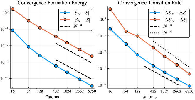
Figure 1. Convergence of energy and entropy contributions to formation energy $\mathcal{F}_{N}$ and transition rate $\mathcal{K}_{N}$, for a vacancy defect in bcc tungsten (W) modelled by a Finnis-Sinclair (EAM) potential [WZLH13], employing a cubic computational cell, i.e., ${\sf B}\propto I$.

3. Resolvent Estimates

3.1. Notation / Preliminaries

Let us fix some more notation.

• $|r|$ is the standard Euclidean norm and

  $$|r|^{-n}_{l^{k}}:=(|r|+1)^{-n}\log^{k}(e+|r|),$$ (3.1)

  where $r$ can be a vector or scalar. For $M>0$, we extend the definition by setting

  $$\lvert n\rvert_{l^{k},M}^{-d}=\min\big{\{}\lvert n\rvert_{l^{k}}^{-d},\lvert M\rvert_{l^{k}}^{-d}\big{\}}.$$

• For $m,n\in\Lambda$ and $M>0,k\geq 0$ we then define

  $$\mathscr{L}_{k}(n,m) :=|n|_{l^{k}}^{-d}|n-m|_{l^{k}}^{-d}+|m|_{l^{k}}^{-d}|n-m|_{l^{k}}^{-d}+|n|_{l^{k}}^{-d}|m|_{l^{k}}^{-d},$$ (3.2)

  $$\mathscr{L}_{k}^{M}(n,m) :=\lvert n\rvert_{l^{k},M}^{-d}\lvert n-m\rvert_{l^{k}}^{-d}+\lvert m\rvert_{l^{k},M}^{-d}\lvert n-m\rvert_{l^{k}}^{-d}+\lvert n\rvert_{l^{k},M}^{-d}\lvert m\rvert_{l^{k},M}^{-d}.$$ (3.3)

• We use the semi-discrete Fourier transform

  $$\hat{u}(k):=\sum_{\ell\in\Lambda}e^{ik\cdot\ell}u(\ell),\quad\text{with inverse}\quad u(\ell)=\frac{1}{\lvert\mathcal{B}\rvert}\int_{\mathcal{B}}e^{-ik\cdot\ell}\hat{u}(k)\,dk,$$ (3.4)

  where $\mathcal{B}=\pi{\sf A}^{-T}(-1,1)^{d}$ is a fundamental domain of reciprocal space (equivalent to the first Brillouin zone) and has the volume $\lvert\mathcal{B}\rvert=\frac{(2\pi)^{d}}{\lvert\det{\sf A}\rvert}$.

3.2. Estimate of ${\bf F}$

We begin by defining and establishing decay estimates for the operator ${\bf F}$. Since $H^{\rm hom}$ is circulant, it is natural to formally represent ${\bf F}w=F\ast w$ and define $F$ via its Fourier transform. First, recall that

$$\langle H^{\rm hom}u,v\rangle=\sum_{\ell\in\mathbb{Z}^{d}}\nabla^{2}V(0)[Du(\ell),Dv(\ell)],$$

then applying the SDFT we obtain

$$\langle H^{\rm hom}u,v\rangle =\frac{1}{\lvert\mathcal{B}\rvert}\int_{\mathcal{B}}\hat{u}(k)^{*}\hat{h}(k)\hat{v}(k)\,dk,$$ (3.5)

$$a^{T}\hat{h}(k)b :=\nabla^{2}V(0)[((e^{-ik\cdot\rho}-1)a)_{\rho\in\mathcal{R}},((e^{ik\cdot\rho}-1)b)_{\rho\in\mathcal{R}}].$$

One can also reduce $\hat{h}(k)$ to the simpler form

$$\hat{h}(k)=4\sum_{\rho\in\mathcal{R}^{\prime}}A_{\rho}\sin^{2}\big{(}{\textstyle\frac{k\cdot\rho}{2}}\big{)},$$ (3.6)

with $\mathcal{R}^{\prime}=(\mathcal{R}\cup\{0\})+(\mathcal{R}\cup\{0\})$, see [EOS16, Sec. 6.2]. Furthermore, (STAB) implies that $c_{0}|k|^{2}I\leq\hat{h}(k)\leq c_{1}|k|^{2}I$ in the matrix sense for all $k\in\mathcal{B}$, see [HO12]. We observe that $|\hat{h}(k)^{-1/2}|\lesssim|k|^{-1}$ as $|k|\to 0$, hence we can define

$$F(\ell) :=\frac{1}{\lvert\mathcal{B}\rvert}\int_{\mathcal{B}}e^{-ik\cdot\ell}\hat{F}(k)\,dk,\qquad\text{where}\quad\hat{F}(k)=\hat{h}(k)^{-1/2},$$ (3.7)

$$({\bf F}u)(\ell) :=\sum_{m\in\Lambda}\big{(}F(\ell-m)-F(-m)\big{)}u(m).$$ (3.8)

The constant shift $\sum_{m}F(-m)u(m)$ in the definition of ${\bf F}u$ ensures that ${\bf F}u$ is well-defined (when $d=2$ the separate sums need not converge).

Lemma 3.1.

Let $F:\Lambda\to\mathbb{R}^{m\times m}$ be defined by (3.7) and ${\bf F}$ by (3.8), then

1. For any $\boldsymbol{\rho}\in\mathcal{R}^{j}$, $j\geq 0$, there exists a constant $C$ such that

   $$|D_{\boldsymbol{\rho}}F(\ell)|\leq C|\ell|_{l^{0}}^{1-d-j}\quad\forall\ell\in\mathbb{Z}^{d}.$$

2. ${\bf F}\in\mathcal{L}(\ell^{2},\dot{\mathcal{W}}^{1,2})$.

3. ${\bf F}^{*}H^{\rm hom}{\bf F}=I$, understood as operators $\ell^{2}\to\ell^{2}$.

Proof.

Our argument closely follows the Green’s function estimate of [EOS16], adapted to the fact that $F$ is the square-root of a Green’s function. The details are given in § 7.1. ∎

3.3. Functional calculus

Suppose that $A:\ell^{2}\to\ell^{2}$ is a bounded, self-adjoint operator with $\sigma(A)\subset[\underline{\sigma},\overline{\sigma}]$, $0<\underline{\sigma}<1<\overline{\sigma}$, and $\mathcal{C}$ is a contour that encloses $[\underline{\sigma},\overline{\sigma}]$, but not the origin, then [DS58, Ch. VII.3]

$$\log A:=\frac{1}{2\pi i}\oint_{\mathcal{C}}\log z(z-A)^{-1}\,dz$$

defines a bounded, self-adjoint operator on $\ell^{2}$. More generally, let $A:\ell^{2}\to\ell^{2}$ be bounded, self-adjoint with $\sigma(A)\cap(0,\infty)\subset[\underline{\sigma},\overline{\sigma}]$, we can use the same contour to define

$$\log^{+}A:=\frac{1}{2\pi i}\oint_{\mathcal{C}}\log z(z-A)^{-1}\,dz.$$ (3.9)

This generalisation will be crucial to be able to apply the subsequent analysis not only to the formation free energy (Theorem 2.6), but also to the analysis of transition rates (Theorem 2.8). As clearly $\log A=\log^{+}A$ in the case that $\sigma(A)\subset[\underline{\sigma},\overline{\sigma}]$, it suffices to consider $\log^{+}A$ in the following.

In order to apply this in our setting we substitute $A={\bf F}^{*}H^{t}(u){\bf F}$, where

$$H^{t}(u):=(1-t)H^{\rm hom}+tH(u),\qquad t\in[0,1],$$

for $u$ in a neighbourhood of $\bar{u}$. Our first step is therefore to show that these operators remain uniformly bounded above and below.

Lemma 3.2.

Let $\bar{u}$ be a stable minimiser of $\mathcal{E}$, then there exist $\epsilon,\underline{\sigma},\overline{\sigma}>0$ such that, for all $u\in B_{\epsilon}(\bar{u})\subset\dot{\mathcal{W}}^{1,2}$ and $t\in[0,1]$,

$$\sigma\big{[}{\bf F}^{*}H^{t}(u){\bf F}\big{]}\subset[\underline{\sigma},\overline{\sigma}].$$ (3.10)

More generally, assume $u_{\infty}\in\dot{\mathcal{W}}^{1,2}$ satisfies $\sigma({\bf F}^{*}H^{t}(u_{\infty}){\bf F})\cap(-\underline{\sigma},\infty)\subset[2\underline{\sigma},\overline{\sigma}/2]$ for some $0<\underline{\sigma}<\overline{\sigma}$, then

$$\sigma\big{[}{\bf F}^{*}H^{t}(u){\bf F}\big{]}\cap(0,\infty)\subset[\underline{\sigma},\overline{\sigma}].$$ (3.11)

for all $u\in B_{\epsilon}(u_{\infty})\subset\dot{\mathcal{W}}^{1,2}$ and $t\in[0,1]$.

Proof.

According to (STAB) we have

$$c_{0}\|Dv\|_{\ell^{2}}^{2}\leq\langle H^{t}(\bar{u})v,v\rangle\leq c_{1}\|Dv\|_{\ell^{2}}^{2}.$$ (3.12)

Hence, $H^{t}(\bar{u})\in\mathcal{L}(\dot{\mathcal{W}}^{1,2},(\dot{\mathcal{W}}^{1,2})^{*})$ and Lemma 3.1 implies that ${\bf F}^{*}H^{t}(\bar{u}){\bf F}\in\mathcal{L}(\ell^{2},\ell^{2})$. Since ${\bf F}^{*}H^{\rm hom}{\bf F}=I$ (see again Lemma 3.1) it follows that

$$c_{0}\|D{\bf F}w\|_{\ell^{2}}^{2}\leq\langle{\bf F}^{*}H^{\rm hom}{\bf F}w,w\rangle=\|w\|_{\ell^{2}}^{2}\leq c_{1}\|D{\bf F}w\|_{\ell^{2}}^{2}.$$

Substituting $v={\bf F}w$ into (3.12) we obtain

$${\textstyle\frac{c_{0}}{c_{1}}}\|w\|_{\ell^{2}}^{2}\leq\langle H^{t}(\bar{u}){\bf F}w,{\bf F}w\rangle=\langle{\bf F}^{*}H^{t}(\bar{u}){\bf F}w,w\rangle\leq{\textstyle\frac{c_{1}}{c_{0}}}\|w\|_{\ell^{2}}^{2}.$$

If now $u\in B_{\epsilon}(\bar{u})$, we use the assumption $V_{\ell}\in C^{3}$ to estimate

$$\Big{\lvert}\big{\langle}(H^{t}(u)-H^{t}(\bar{u})){\bf F}w,{\bf F}w\big{\rangle}\Big{\rvert} \lesssim\lVert D{\bf F}w\rVert_{\ell^{2}}^{2}\lVert Du-D\bar{u}\rVert_{\ell^{\infty}}\lesssim\epsilon\lVert w\rVert_{\ell^{2}}^{2},$$

which proves the remaining claims. ∎

In light of the foregoing lemma, there exists a contour $\mathcal{C}$ encircling $[\underline{\sigma},\overline{\sigma}]$ but not the origin, such that, for $u\in B_{\epsilon}(u_{\infty})$ and for all $t\in[0,1]$,

$$\log^{+}\big{[}{\bf F}^{*}H^{t}(u){\bf F}\big{]}=\frac{1}{2\pi i}\oint_{\mathcal{C}}\log z\,\mathscr{R}^{t}_{z}(u)\,dz,\quad\text{where }\mathscr{R}^{t}_{z}=\mathscr{R}^{t}_{z}(u):=(z-{\bf F}^{*}H^{t}(u){\bf F})^{-1}.$$ (3.13)

From now on, we will fix this contour and always have $z\in\mathcal{C}$ and $t\in[0,1]$. We will also use the notation $\mathscr{R}^{\rm hom}_{z}:=\mathscr{R}^{0}_{z}(u)$ and $\mathscr{R}_{z}(u):=\mathscr{R}^{1}_{z}(u)$. We remark that, since ${\bf F}^{*}H^{\rm hom}{\bf F}=I$, we have $\mathscr{R}^{\rm hom}_{z}=(z-I)^{-1}=(z-1)^{-1}I$.

To exploit the representation (3.13) we will analyse the resolvents $\mathscr{R}_{z}^{t}$. Specifically, we will estimate how $[\mathscr{R}^{t}_{z}]_{\ell n}$ decays as $|\ell|,|n|\to\infty$.

3.4. Finite-rank corrections

A basic technique that we will employ in the resolvent decay estimates is to decompose a Hessian operator $H$ into two components $H=H_{\rm r}+H_{\rm h}$ where $H_{\rm r}$ has finite rank while $H_{\rm h}$ is close to $H^{\rm hom}$. To estimate the correction to the resolvent due to $H_{\rm r}$, the following lemma shows that we can instead estimate powers of the finite rank correction.

Lemma 3.3.

Let $X$ be a Hilbert space.

1. Let $A\in\mathcal{L}(X,X)$ be a bounded linear operator with range of finite dimension at most $r\in\mathbb{N}$ and $I+A$ is invertible, then there exist $c_{1}(A),\dots,c_{r+1}(A)\in\mathbb{R}$ such that

   $$(I+A)^{-1}=I+\sum_{j=1}^{r+1}c_{j}(A)A^{j}.$$ (3.14)

   If $U\subset\mathbb{C}$ such that $(I+\gamma A)$ is invertible for all $\gamma\in U$, then $\gamma\mapsto c_{j}(\gamma A)$ are continuous functions on $U$.

2. More generally, let $X=X_{1}\oplus X_{2}$ be a fixed orthogonal decomposition with ${\rm dim}(X_{1})\leq r$ then (3.14) holds for all $A$ for which $X_{2}\subset{\rm ker}A$ and $(I+A)$ is invertible. The coefficients can be written as $c_{j}(A)=d_{j}(\pi_{X_{1}}A|_{X_{1}})$ where $\pi_{X_{1}}A|_{X_{1}}\colon X_{1}\to X_{1}$ is the restriction and projection of $A$ to $X_{1}$ and the $d_{j}$ are continuous on the finite-dimensional set $\{B\in\mathcal{L}(X_{1},X_{1})\colon(I+B)\text{ is invertible}\}$.

Proof.

The result is a consequence of the Cayley–Hamilton theorem; we give the complete proof in § 7.2. ∎

3.5. Resolvent estimates

The goal of this section is to estimate $\mathscr{R}^{t}_{z}(u)=(z-{\bf F}^{*}H^{t}(u){\bf F})^{-1}$, where

$$u\in\mathcal{U}:=\mathcal{U}(\underline{\sigma},\overline{\sigma},C):=\big{\{}u\in\dot{\mathcal{W}}^{1,2}\,:\,u\text{ satisfies }\eqref{eq:logpluscondition}\text{ with }\underline{\sigma},\overline{\sigma}\ \text{ and }\ |Du(\ell)|\leq C|\ell|_{l^{0}}^{-d}\big{\}}.$$

This more stringent condition is sufficient for our purposes and considerably simplifies several proofs. In particular, $C,\overline{\sigma}>0$ sufficiently large and $\underline{\sigma}>0$ sufficiently small are fixed throughout this discussion and all constants in the following are allowed to depend on them.

As already hinted to above, a key idea is to split the difference of the Hamiltonians $H(u)-H^{\rm hom}$ into a sum of a large finite rank operator representing the defect core and a small but infinite rank part representing the far field. Let

$$\langle H^{M}(u)v,z\rangle=\sum_{\lvert\ell\rvert\leq M}\nabla^{2}V(0)[Dv(\ell),Dz(\ell)]+\sum_{\lvert\ell\rvert>M}\nabla^{2}V(Du(\ell))[Dv(\ell),Dz(\ell)],$$ (3.15)

and define $H^{M,t}(u):=(1-t)H^{\rm hom}+tH^{M}(u)$ and $\mathscr{R}^{M,t}_{z}$ analogously. Then,

$$\begin{split}\mathscr{R}^{M,t}_{z}(u)-\mathscr{R}^{\rm hom}_{z}&=\Big{(}(z-1)I-t{\bf F}^{*}\big{(}H^{M}(u)-H^{\rm hom}\big{)}{\bf F}\Big{)}^{-1}-(z-1)^{-1}I\\ &=(z-1)^{-1}\bigg{\{}\Big{(}I-{\textstyle\frac{t}{z-1}}{\bf F}^{*}\big{(}H^{M}(u)-H^{\rm hom}\big{)}{\bf F}\Big{)}^{-1}-I\bigg{\}}.\end{split}$$ (3.16)

We now show that $A_{M}:={\bf F}^{*}(H^{M}(u)-H^{\rm hom}){\bf F}$ is small provided that $M$ is sufficiently large. Starting with this lemma, we will heavily rely on the convenient notation $\lvert\ell\lvert^{-d}_{l^{k}}$ defined in (3.1) for a decay rate up to $k$ logarithmic factors, as well as the notation $\mathscr{L}_{k}$ and $\mathscr{L}_{k}^{M}$ defined in (3.2) and (3.3) for operator estimates.

Lemma 3.4.

There exist $C_{0},C_{1},C_{2}>0$ independent of $m$, $n$, $M$, and $u\in\mathcal{U}$ such that

$$\lvert(A_{M})_{mn}\rvert \leq C_{0}\mathscr{L}_{1}^{M}(m,n),\qquad\text{where}$$ (3.17)

$$\sum\limits_{m,n\in\Lambda}\mathscr{L}_{1}^{M}(m,n)^{2} \leq C_{1}\lvert M\rvert_{l^{3}}^{-d},\qquad\text{and}$$ (3.18)

$$\sum\limits_{\ell\in\Lambda}\mathscr{L}_{1}^{M}(m,\ell)\mathscr{L}_{1}^{M}(\ell,n) \leq C_{2}\lvert M\rvert_{l^{3}}^{-d}\mathscr{L}_{1}^{M}(m,n).$$ (3.19)

Proof.

Many detailed sums we need here and in the following are collected in the appendix in Section 7.3. Specifically, (7.13) yields (3.17):

$$\lvert(A_{M})_{mn}\rvert \leq\sum_{\lvert\ell\rvert>M}\lvert\nabla^{2}V(Du(\ell))-\nabla^{2}V(0)\rvert\lvert DF(\ell-m)\rvert\lvert DF(\ell-n)\rvert$$

$$\lesssim\sum_{\lvert\ell\rvert>M}\lvert\ell\rvert_{l^{0}}^{-d}\lvert\ell-m\rvert_{l^{0}}^{-d}\lvert\ell-n\rvert_{l^{0}}^{-d}$$

$$\lesssim\mathscr{L}_{1}^{M}(m,n).$$

For (3.19) we estimate

$$\sum_{\ell\in\Lambda}\mathscr{L}_{1}^{M}(m,\ell)\mathscr{L}_{1}^{M}(\ell,n) \lesssim\lvert n\rvert_{l^{1},M}^{-d}\lvert m\rvert_{l^{1},M}^{-d}\sum_{\ell\in\Lambda}(\lvert\ell\rvert_{l^{1},M}^{-d}+\lvert m-\ell\rvert_{l^{1}}^{-d})(\lvert\ell\rvert_{l^{1},M}^{-d}+\lvert n-\ell\rvert_{l^{1}}^{-d})$$

$$\quad+\lvert n\rvert_{l^{1},M}^{-d}\sum_{\ell\in\Lambda}\lvert\ell\rvert_{l^{1},M}^{-d}\lvert m-\ell\rvert_{l^{1}}^{-d}(\lvert\ell\rvert_{l^{1},M}^{-d}+\lvert n-\ell\rvert_{l^{1}}^{-d})$$

$$\quad+\lvert m\rvert_{l^{1},M}^{-d}\sum_{\ell\in\Lambda}\lvert\ell\rvert_{l^{1},M}^{-d}\lvert n-\ell\rvert_{l^{1}}^{-d}(\lvert\ell\rvert_{l^{1},M}^{-d}+\lvert m-\ell\rvert_{l^{1}}^{-d})$$

$$\quad+\sum_{\ell\in\Lambda}\lvert\ell\rvert_{l^{2},M}^{-2d}\lvert m-\ell\rvert_{l^{1}}^{-d}\lvert n-\ell\rvert_{l^{1}}^{-d}.$$ (3.20)

We look at each of the sums in detail. According to (7.5) and (7.7) we have the estimates

$$\sum_{\ell\in\Lambda}\lvert\ell\rvert_{l^{2},M}^{-2d} \lesssim\lvert M\rvert_{l^{2}}^{-d},$$

$$\sum_{\ell\in\Lambda}\lvert\ell\rvert_{l^{1},M}^{-d}\lvert n-\ell\rvert_{l^{1}}^{-d} \lesssim\lvert n\rvert_{l^{3},M}^{-d}\lesssim\lvert M\rvert_{l^{3}}^{-d},$$

$$\sum_{\ell\in\Lambda}\lvert m-\ell\rvert_{l^{1}}^{-d}\lvert\ell\rvert_{l^{1},M}^{-d} \lesssim\lvert m\rvert_{l^{3},M}^{-d}\lesssim\lvert M\rvert_{l^{3}}^{-d},$$

$$\sum_{\ell\in\Lambda}\lvert m-\ell\rvert_{l^{1}}^{-d}\lvert n-\ell\rvert_{l^{1}}^{-d} \lesssim\lvert n-m\rvert_{l^{3}}^{-d},$$

Furthermore, according to (7.8) and (7.14) we also have

$$\sum_{\ell\in\Lambda}\lvert\ell\rvert_{l^{2},M}^{-2d}\lvert m-\ell\rvert_{l^{1}}^{-d} \lesssim\lvert m\rvert_{l^{1},M}^{-d}\lvert M\rvert_{l^{3}}^{-d},$$

$$\sum_{\ell\in\Lambda}\lvert\ell\rvert_{l^{1},M}^{-d}\lvert m-\ell\rvert_{l^{1}}^{-d}\lvert n-\ell\rvert_{l^{1}}^{-d} \lesssim\lvert m\rvert_{l^{1},M}^{-d}\lvert n\rvert_{l^{3},M}^{-d}+\lvert m-n\rvert_{l^{3}}^{-d}\lvert m\rvert_{l^{1},M}^{-d},$$

and analogously for $m$ and $n$ reversed. At last, according to (7.16), we also have

$$\sum\limits_{\ell\in\Lambda}\lvert\ell\rvert_{l^{2},M}^{-2d}\lvert\ell-n\rvert_{l^{1}}^{-d}\lvert\ell-m\rvert_{l^{1}}^{-d}\lesssim\lvert n\rvert_{l^{1},M}^{-d}\lvert m\rvert_{l^{1},M}^{-d}(\lvert M\rvert_{l^{3}}^{-d}+\lvert m-n\rvert_{l^{3}}^{-d}).$$

Inserting these intermediate estimates into (3.20) we get (3.19), as

$$\sum\limits_{\ell\in\Lambda}\mathscr{L}_{1}^{M}(m,\ell)\mathscr{L}_{1}^{M}(\ell,n) \lesssim\lvert n\rvert_{l^{1},M}^{-d}\lvert m\rvert_{l^{1},M}^{-d}(\lvert M\rvert_{l^{3}}^{-d}+\lvert m-n\rvert_{l^{3}}^{-d})$$ (3.21)

$$\lesssim\lvert M\rvert_{l^{3}}^{-d}\mathscr{L}_{1}^{M}(m,n).$$

Finally, summing over $m=n$ in (3.21), and using (7.5), we deduce (3.18):

$$\sum\limits_{m\in\Lambda}\sum\limits_{\ell\in\Lambda}\mathscr{L}_{1}^{M}(m,\ell)\mathscr{L}_{1}^{M}(\ell,m) \lesssim\sum\limits_{m\in\Lambda}\lvert m\rvert_{l^{2},M}^{-2d}\lesssim\lvert M\rvert_{l^{3}}^{-d}.\qed$$

Proposition 3.5.

There exists a constant $C_{3}>0$ such that, for all $u\in\mathcal{U}$, $t\in[0,1]$, $z\in\mathcal{C}$,

$$\Big{|}\big{[}\mathscr{R}_{z}^{t}(u)-\mathscr{R}^{\rm hom}_{z}\big{]}_{minj}\Big{|}\leq C_{3}\mathscr{L}_{1}(m,n).$$ (3.22)

Proof.

We split $\mathscr{R}_{z}^{t}-\mathscr{R}^{\rm hom}_{z}=(\mathscr{R}_{z}^{t}-\mathscr{R}^{M,t}_{z})+(\mathscr{R}^{M,t}_{z}-\mathscr{R}^{\rm hom}_{z})$. To estimate the first group we will use that $H^{t}-H^{M,t}$ has finite rank. To estimate the second group we will use that $H^{M,t}-H^{\rm hom}$ is small.

We begin by estimating $\mathscr{R}^{M,t}_{z}-\mathscr{R}^{\rm hom}_{z}$. Recall from (3.16) that

$$\mathscr{R}^{M,t}_{z}(u)-\mathscr{R}^{\rm hom}_{z}=(z-1)^{-1}\Big{(}\Big{(}I-{\textstyle\frac{t}{z-1}}A_{M}\Big{)}^{-1}-I\Big{)},$$

with $A_{M}={\bf F}^{*}(H^{M}(u)-H^{\rm hom}(0)){\bf F}$.

We can show that for $M$ sufficiently large the associated Neumann series converges, from which we can deduce not only that $(I-\frac{t}{z-1}A_{M})^{-1}$ (and hence also $\mathscr{R}^{M,t}_{z}(u)$) is well-defined but also obtain decay estimates. Indeed, we can bound the Frobenius norm by

$$\lVert A_{M}\rVert_{F}^{2} \leq C_{0}^{2}d^{2}\sum_{m,n\in\Lambda}\mathscr{L}_{1}^{M}(m,n)^{2}\leq C_{0}^{2}d^{2}C_{1}\lvert M\rvert^{-d}_{l^{3}},$$

according to Lemma 3.4. As the Frobenius norm is sub-multiplicative, for $M$ sufficiently large, the Neumann series

$$\Big{(}I-{\textstyle\frac{t}{z-1}}A_{M}\Big{)}^{-1}=\sum_{k=0}^{\infty}\frac{t^{k}}{(z-1)^{k}}A_{M}^{k}$$

converges strongly in the Frobenius norm, uniformly in $z\in\mathcal{C},t\in[0,1]$ and $u\in\mathcal{U}_{\epsilon}$. From Lemma 3.4 we can moreover deduce that

$$\lvert(A_{M}^{k})_{mn}\rvert\leq(dC_{2}\lvert M\rvert_{l^{3}}^{-d})^{k-1}C_{0}^{k}\mathscr{L}_{1}^{M}(m,n),$$

and hence

$$\bigg{|}\sum_{k=0}^{\infty}\frac{t^{k}(A_{M}^{k})_{mn}}{(z-1)^{k}}-I_{mn}\bigg{|} \leq\mathscr{L}_{1}^{M}(n,m)\sum_{k=1}^{\infty}\frac{C_{0}^{k}C_{2}^{k-1}d^{k-1}(\lvert M\rvert_{l^{3}}^{-d})^{k-1}}{\lvert z-1\rvert^{k}}.$$

For $M$ large enough the series on the right-hand side converges uniformly in $z$, and therefore

$$\Big{|}\big{[}\mathscr{R}^{M,t}_{z}(u)-\mathscr{R}^{\rm hom}_{z}\big{]}_{mn}\Big{|}\lesssim\mathscr{L}_{1}^{M}(m,n).$$ (3.23)

It remains to estimate $\mathscr{R}^{t}_{z}-\mathscr{R}^{M,t}_{z}$. We begin by rewriting

$$\mathscr{R}_{z}^{t}(u)=\Big{(}I+\mathscr{R}^{M,t}_{z}(u){\bf F}^{*}\big{(}H^{M,t}(u)-H^{t}(u)\big{)}{\bf F}\Big{)}^{-1}\mathscr{R}^{M,t}_{z}(u)=:\big{(}I+B^{M,t}\big{)}^{-1}\mathscr{R}^{M,t}_{z}(u).$$

Lemma 3.2 implies that the resolvent $\mathscr{R}_{z}^{t}(u)$ exists for all $z\in\mathcal{C},t\in[0,1],u\in\mathcal{U}$ and hence the inverse on the right hand side exists as well.

Moreover, $B^{M,t}$ has finite-dimensional range since clearly this is the case for $H^{M,t}(u)-H^{t}(u)$. More precisely, if we set $X_{2}=\{u\in\ell^{2}\colon D({\bf F}u)(\ell)=0\text{ for all }\lvert\ell\rvert\leq M\}$, then $X_{2}\subset{\rm ker}(B^{M,t})$, while $X_{1}:=X_{2}^{\perp}$ is finite dimensional. According to Lemma 3.3 it follows that

$$\big{(}I+B^{M,t}\big{)}^{-1}=I+\sum_{j=1}^{r+1}\big{(}B^{M,t}\big{)}^{j}d_{j},$$ (3.24)

with $d_{j}$ depending continuously on the projected and restricted operators $\pi_{X_{1}}B^{M,t}|_{X_{1}}$. In particular, these constants remain uniformly bounded in $z,t$ and $u\in\mathcal{U}$. Therefore, we only have to estimate

$$\big{(}B^{M,t}\big{)}^{j}\mathscr{R}^{M,t}_{z}=\Big{(}\mathscr{R}^{M,t}_{z}{\bf F}^{*}(H^{M,t}-H^{t}){\bf F}\Big{)}^{j}\mathscr{R}^{M,t}_{z}$$

for $1\leq j\leq r+1$. To that end, we note that similarly as in Lemma 3.4

$$\lvert({\bf F}^{*}(H^{t,M}-H^{t}){\bf F})_{mn}\rvert \lesssim t\sum_{\lvert\ell\rvert\leq M}\lvert\ell\rvert_{l^{0}}^{-d}\lvert\ell-m\rvert_{l^{0}}^{-d}\lvert\ell-n\rvert_{l^{0}}^{-d}$$

$$\leq\sum_{\ell}\lvert\ell\rvert_{l^{0}}^{-d}\lvert\ell-m\rvert_{l^{0}}^{-d}\lvert\ell-n\rvert_{l^{0}}^{-d}$$

$$\lesssim\mathscr{L}_{1}(m,n),$$ (3.25)

based on (7.13). Recall also from (3.23) that

$$\lvert(\mathscr{R}^{M,t}_{z}(u)-\mathscr{R}^{\rm hom}_{z})_{mn}\rvert\lesssim\mathscr{L}_{1}^{M}(m,n)\leq\mathscr{L}_{1}(m,n),$$ (3.26)

hence we can now use (3.19) with $M=0$ to deduce

$$\Big{|}\big{[}\big{(}\mathscr{R}^{M,t}_{z}(u){\bf F}^{*}(H^{t,M}-H^{t}){\bf F}\big{)}^{j}\mathscr{R}^{M,t}_{z}(u)\big{]}_{mn}\Big{|}\lesssim\mathscr{L}_{1}(m,n),$$

where the implied constant is independent of $z\in\mathcal{C},t\in[0,1]$ and $u\in\mathcal{U}$. Combined with (3.24) this completes the proof. ∎

4. Locality Estimates for $S$

In the following, will use the definition

$$\mathcal{S}^{+}_{\ell}(u):=-{\textstyle\frac{1}{2}}{\rm Trace}\Big{[}\log^{+}\big{(}{\bf F}^{*}H(u){\bf F}\big{)}\Big{]}_{\ell\ell},$$ (4.1)

for $u$ satisfying (3.11). Of course, we have $\mathcal{S}^{+}_{\ell}(u)=\mathcal{S}_{\ell}(u)$ included as a special case if (3.10) is true.

Let us start with the regularity claim.

Proof of Theorem 2.6 (1).

According to Lemma 2.1, $H(u),H^{\rm hom}(u):\dot{\mathcal{W}}^{1,2}\to\mathcal{L}(\dot{\mathcal{W}}^{1,2},(\dot{\mathcal{W}}^{1,2})^{\prime})$ are $(p-2)$-times continuously Fréchet differentiable. Due to Lemma 3.1 and Lemma 3.2, $\mathscr{R}^{\rm hom}_{z}(0)$ and $\mathscr{R}_{z}(\bar{u})$ exist. As the set of invertible linear operators is open and inverting is smooth, we find that $\mathscr{R}^{\rm hom}_{z}(u),\mathscr{R}_{z}(\bar{u}+u):B_{\delta}(0)\subset\dot{\mathcal{W}}^{1,2}\to\mathcal{L}(\ell^{2},\ell^{2})$ to be $(p-2)$-times continuously Fréchet differentiable for $\delta>0$ small enough. All of this can be done uniformly in $z\in\mathcal{C}$. Therefore, the same regularity holds true for $\log\big{(}{\bf F}^{*}H(u){\bf F}\big{)}$, $\log\big{(}{\bf F}^{*}H^{\rm hom}(u){\bf F}\big{)}$, and any of their components. ∎

Based on $H^{t}(u)=(1-t)H^{\rm hom}(0)+tH(u)$ for $u\in\mathcal{U}$, define

$$\SS_{\ell}^{t}(u):=-{\textstyle\frac{1}{2}}{\rm Trace}\Big{[}\log^{+}\big{(}{\bf F}^{*}H^{t}(u){\bf F}\big{)}\Big{]}_{\ell\ell},$$

then

$$\SS^{+}_{\ell}(u)=\SS_{\ell}^{0}(u)+\frac{\partial\SS_{\ell}^{0}(u)}{\partial t}+\int_{0}^{1}(1-t)\frac{\partial^{2}\SS_{\ell}^{t}(u)}{\partial^{2}t}\,dt.$$

Indeed, we directly check that $t\mapsto\SS_{\ell}^{t}$ is twice differentiable with

$$\frac{\partial\SS_{\ell}^{t}(u)}{\partial t}=-\frac{1}{2}\frac{1}{2\pi i}\oint_{\mathcal{C}}\log z\,{\rm Trace}\big{(}\mathscr{R}_{z}^{t}{\bf F}^{*}(H(u)-H^{\rm hom}(0)){\bf F}\mathscr{R}_{z}^{t}\big{)}_{\ell\ell}\,dz$$

and

$$\frac{\partial^{2}\SS_{\ell}^{t}(u)}{\partial t^{2}}=-\frac{1}{2}2\frac{1}{2\pi i}\oint_{\mathcal{C}}\log z\,{\rm Trace}\big{(}\mathscr{R}_{z}^{t}{\bf F}^{*}(H(u)-H^{\rm hom}(0)){\bf F}\mathscr{R}_{z}^{t}{\bf F}^{*}(H(u)-H^{\rm hom}(0)){\bf F}\mathscr{R}_{z}^{t}\big{)}_{\ell\ell}\,dz.$$

In particular, we find $\SS_{\ell}^{0}(u)=0$ and

$$\frac{\partial\SS_{\ell}^{0}(u)}{\partial t} =-\frac{1}{2}\frac{1}{2\pi i}\oint_{\mathcal{C}}\frac{\log z}{(z-1)^{2}}{\rm Trace}\big{(}{\bf F}^{*}(H(u)-H^{\rm hom}(0)){\bf F}\big{)}_{\ell\ell}\,dz$$

$$=-\frac{1}{2}{\rm Trace}\big{(}{\bf F}^{*}(H(u)-H^{\rm hom}(0)){\bf F}\big{)}_{\ell\ell}.$$

We can then write

$$\frac{\partial\SS_{\ell}^{0}(u)}{\partial t} =-\frac{1}{2}{\rm Trace}\big{(}{\bf F}^{*}\langle\delta H^{\rm hom}(0),u\rangle{\bf F}\big{)}_{\ell\ell}$$

$$\quad-\frac{1}{2}\int_{0}^{1}(1-s){\rm Trace}\big{(}{\bf F}^{*}\langle\delta^{2}H^{\rm hom}(su)u,u\rangle{\bf F}\big{)}_{\ell\ell}\,ds$$

$$\quad-\frac{1}{2}{\rm Trace}\big{(}{\bf F}^{*}\big{(}H(u)-H^{\rm hom}(u)\big{)}{\bf F}\big{)}_{\ell\ell}.$$

Also note that

$$\langle\delta\SS^{\rm hom}_{\ell}(0),u\rangle =-\frac{1}{2}\frac{1}{2\pi i}\oint_{\mathcal{C}}\log z\,{\rm Trace}\big{(}\mathscr{R}^{\rm hom}_{z}{\bf F}^{*}\langle\delta H^{\rm hom}(0),u\rangle{\bf F}\mathscr{R}^{\rm hom}_{z}\big{)}_{\ell\ell}\,dz$$

$$=-\frac{1}{2}{\rm Trace}\big{(}{\bf F}^{*}\langle\delta H^{\rm hom}(0),u\rangle{\bf F}\big{)}_{\ell\ell}.$$

Overall, we have decomposed $\SS^{+}_{\ell}(u)$ into

$$\SS^{+}_{\ell}(u)=\langle\delta\SS^{\rm hom}_{\ell}(0),u\rangle+\SS_{\ell,1}(u)+\SS_{\ell,2}(u)+\SS_{\ell,3}(u),$$ (4.2)

with

$$\SS_{\ell,1}(u) :=-\frac{1}{2}\int_{0}^{1}(1-s){\rm Trace}\big{(}{\bf F}^{*}\langle\delta^{2}H^{\rm hom}(su)u,u\rangle{\bf F}\big{)}_{\ell\ell}\,ds,$$

$$\SS_{\ell,2}(u) :=-\frac{1}{2}{\rm Trace}\big{(}{\bf F}^{*}\big{(}H(u)-H^{\rm hom}(u)\big{)}{\bf F}\big{)}_{\ell\ell},$$

$$\SS_{\ell,3}(u) :=-\frac{1}{2}\int_{0}^{1}\oint_{\mathcal{C}}(1-t)\frac{2}{2\pi i}\log z$$

$$\qquad{\rm Trace}\big{(}\mathscr{R}_{z}^{t}{\bf F}^{*}(H(u)-H^{\rm hom}(0)){\bf F}\mathscr{R}_{z}^{t}{\bf F}^{*}(H(u)-H^{\rm hom}(0)){\bf F}\mathscr{R}_{z}^{t}\big{)}_{\ell\ell}\,dz\,dt.$$

This decomposition will be useful in light of the properties we establish next:

Proposition 4.1.

For $u\in\mathcal{U}$

$$\lvert\langle\delta\SS^{\rm hom}_{\ell}(0),u\rangle\rvert\lesssim\lvert\ell\rvert_{l^{0}}^{-d},$$ (4.3)

but

$$\lvert\SS_{\ell,i}(u)\rvert\lesssim\lvert\ell\rvert_{l^{0}}^{-2d},\quad\text{for }i\in\{1,2\},$$ (4.4)

and

$$\lvert\SS_{\ell,3}(u)\rvert\lesssim\lvert\ell\rvert_{l^{2}}^{-2d}.$$ (4.5)

In particular, the sum

$$\SS^{+}(u):=\sum_{\ell}\Big{(}\SS^{+}_{\ell}(u)-\langle\delta\SS^{\rm hom}_{\ell}(0),u\rangle\Big{)}$$

converges absolutely.

First, let us look more closely at the variations of $H^{\rm hom}$. Remember that $H^{\rm hom}(u)=\delta^{2}\mathcal{E}^{\rm hom}(u)$. We can write its components as

$$H^{\rm hom}(u)_{minj}:=(H^{\rm hom}(u)_{mn})_{ij}=\sum_{\xi\in\Lambda}\nabla^{2}V(Du(\xi))[D(\delta_{m}e_{i})(\xi),D(\delta_{n}e_{j})(\xi)].$$

Accordingly, the first variation is

$$\big{[}\langle\delta H^{\rm hom}(u),v\rangle\big{]}_{minj}=\sum_{\xi\in\Lambda}\nabla^{3}V(Du(\xi))[D(\delta_{m}e_{i})(\xi),D(\delta_{n}e_{j})(\xi),Dv(\xi)].$$

Similarly, for the second variation of $H$ we will use the notation

$$\big{[}\langle\delta^{2}H^{\rm hom}(u)v,w\rangle\big{]}_{minj}=\sum_{\xi\in\Lambda}\nabla^{4}V(Du(\xi))[D(\delta_{m}e_{i})(\xi),D(\delta_{n}e_{j})(\xi),Dv(\xi),Dw(\xi)].$$

Lemma 4.2.

For all $t\in[0,1]$ uniformly, it holds that

$$\Big{\lvert}\big{[}{\bf F}^{*}\langle\delta H^{\rm hom}(tu),v\rangle{\bf F}\big{]}_{mn}\Big{\rvert} \lesssim\sum_{\xi\in\Lambda}|\xi-m|_{l^{0}}^{-d}\,|\xi-n|_{l^{0}}^{-d}\,\lvert Dv(\xi)\rvert,$$ (4.6)

$$\Big{\lvert}\big{[}{\bf F}^{*}\langle\delta^{2}H^{\rm hom}(tu)v,w\rangle{\bf F}\big{]}_{mn}\Big{\rvert} \lesssim\sum_{\xi\in\Lambda}|\xi-m|_{l^{0}}^{-d}\,|\xi-n|_{l^{0}}^{-d}\,\lvert Dv(\xi)\rvert\lvert\,Dw(\xi)\rvert.$$ (4.7)

$$\Big{\lvert}\big{[}{\bf F}^{*}(H(u)-H^{\rm hom}(u)){\bf F}\big{]}_{mn}\Big{\rvert} \lesssim|m|_{l^{0}}^{-d}\,|n|_{l^{0}}^{-d}.$$ (4.8)

Proof.

We have

$$\big{[}{\bf F}^{*}\delta H^{\rm hom}(tu)(\xi){\bf F}\big{]}_{minj}=\nabla^{3}V(tDu(\xi))[DF_{\cdot i}(\xi-m),DF_{\cdot j}(\xi-n)],$$

and $\lvert DF(\xi)\rvert\lesssim\lvert\xi\rvert_{l^{0}}^{-d}$ according to Lemma 3.1. The same is true for the second variation with $\nabla^{4}V$. As $V=V_{\xi}$ for $\lvert\xi\rvert\geq r_{\rm cut}$, we find

$$\Big{\lvert}\big{[}{\bf F}^{*}(H(u)-H^{\rm hom}(u)){\bf F}\big{]}_{minj}\Big{\rvert} \lesssim\sum_{\lvert\xi\rvert<r_{\rm cut}}\Big{(}\nabla^{2}V_{\xi}(Du(\xi))-\nabla^{2}V(Du(\xi))\Big{)}[DF_{\cdot i}(\xi-m),DF_{\cdot j}(\xi-n)]$$

$$\lesssim\sum_{\lvert\xi\rvert<r_{\rm cut}}|\xi-m|_{l^{0}}^{-d}\,|\xi-n|_{l^{0}}^{-d}$$

$$\lesssim|m|_{l^{0}}^{-d}\,|n|_{l^{0}}^{-d}.\qed$$

We now have all the tools to prove Proposition 4.1.

Proof of Proposition 4.1.

Let us begin with the first order term. Using (4.6), $u\in\mathcal{U}$, and (7.8) we find that

$$\lvert\langle\delta\SS^{\rm hom}_{\ell}(0),u\rangle\rvert \lesssim\big{\lvert}\sum_{\xi\in\Lambda}{\rm Trace}\big{(}{\bf F}^{*}\delta H^{\rm hom}(0)(\xi)[Du(\xi)]{\bf F}\big{)}_{\ell\ell}\big{\rvert}$$

$$\lesssim\sum_{\xi\in\Lambda}\lvert\xi-\ell\rvert_{l^{0}}^{-2d}\lvert Du(\xi)\rvert$$

$$\lesssim\sum_{\xi\in\Lambda}\lvert\xi-\ell\rvert_{l^{0}}^{-2d}\lvert\xi\rvert_{l^{0}}^{-d}$$

$$\lesssim\lvert\ell\rvert_{l^{0}}^{-d}.$$

This proves (4.3). Equation (4.4) for $\SS_{\ell,2}(u)$ is already included in (4.8) in Lemma 4.2.

To estimate $\SS_{\ell,1}(u)$ we can use (4.7) and (7.9) to see that

$$\Big{\lvert}\big{(}{\bf F}^{*}\langle\delta^{2}H^{\rm hom}(su)u,u\rangle{\bf F}\big{)}_{\ell\ell}\Big{\lvert} \lesssim\sum_{\xi\in\Lambda}\lvert\xi-\ell\rvert_{l^{0}}^{-2d}\lvert Du(\xi)\rvert^{2}$$

$$\lesssim\sum_{\xi\in\Lambda}\lvert\xi-\ell\rvert_{l^{0}}^{-2d}\lvert\xi\rvert_{l^{0}}^{-2d}$$

$$\lesssim\lvert\ell\rvert_{l^{0}}^{-2d}.$$

The last remaining claim (4.5) requires the resolvent estimates from § 3. We have

$$\SS_{\ell,3}(u) =-\frac{1}{2}\int_{0}^{1}(1-t)\frac{\partial^{2}\SS_{\ell}^{t}(u)}{\partial^{2}t}\,dt$$

$$=-\frac{1}{2}\int_{0}^{1}\oint_{\mathcal{C}}(1-t)\frac{2}{2\pi i}\log z\,{\rm Trace}\big{(}$$

$$\hskip 56.9055pt\mathscr{R}_{z}^{t}{\bf F}^{*}(H(u)-H^{\rm hom}(0)){\bf F}\mathscr{R}_{z}^{t}{\bf F}^{*}(H(u)-H^{\rm hom}(0)){\bf F}\mathscr{R}_{z}^{t}\Big{)}_{\ell\ell}\,dz\,dt.$$

We already know from Proposition 3.5 that

$$\Big{|}\big{(}\mathscr{R}_{z}^{t}(u)-\mathscr{R}^{\rm hom}_{z}\big{)}_{mn}\Big{|}\lesssim\mathscr{L}_{1}(m,n),$$

with $\mathscr{R}^{\rm hom}_{z}=(z-1)^{-1}I$. Furthermore, according to Lemma 4.2 and (7.13)

$$\Big{|}\big{(}{\bf F}^{*}(H(u)-H^{\rm hom}(0)){\bf F}\big{)}_{minj}\Big{|} \lesssim\lvert m\rvert_{l^{0}}^{-d}\lvert n\rvert_{l^{0}}^{-d}+\Big{|}\big{(}{\bf F}^{*}(H^{\rm hom}(u)-H^{\rm hom}(0)){\bf F}\big{)}_{minj}\Big{|}$$

$$\lesssim\lvert m\rvert_{l^{0}}^{-d}\lvert n\rvert_{l^{0}}^{-d}+\sum_{\xi\in\Lambda}\lvert m-\xi\rvert_{l^{0}}^{-d}\lvert n-\xi\rvert_{l^{0}}^{-d}\lvert Du(\xi)\rvert$$

$$\lesssim\lvert m\rvert_{l^{0}}^{-d}\lvert n\rvert_{l^{0}}^{-d}+\sum_{\xi\in\Lambda}\lvert m-\xi\rvert_{l^{0}}^{-d}\lvert n-\xi\rvert_{l^{0}}^{-d}\lvert\xi\rvert_{l^{0}}^{-d}$$

$$\lesssim\mathscr{L}_{1}(m,n).$$

$\mathscr{L}_{1}$ is submultiplicative up to a constant, in the sense that (see Lemma 3.4)

$$\sum_{m}\mathscr{L}_{1}(\ell,m)\mathscr{L}_{1}(m,n)\lesssim\mathscr{L}_{1}(\ell,n).$$

As also

$$\sum_{m}\mathscr{R}^{\rm hom}_{z}(\ell,m)\mathscr{L}_{1}(m,n)\lesssim\mathscr{L}_{1}(\ell,n),$$

we can apply the submultiplicativity several times, and use (3.21), to find

$$\lvert\SS_{\ell,3}(u)\rvert \lesssim\sum_{m\in\Lambda}\mathscr{L}_{1}(\ell,m)\mathscr{L}_{1}(m,\ell)\lesssim\lvert\ell\rvert^{-2d}_{l^{2}}.\qed$$

Proof of Theorem 2.6 (2).

As $\bar{u}\in\mathcal{U}$ with $S^{+}_{\ell}(\bar{u})=S_{\ell}(\bar{u})$ for all $\ell$, we can directly apply Proposition 4.1 to see that

$$\sum_{\ell}\Big{\lvert}\SS_{\ell}(\bar{u})-\langle\delta\SS^{\rm hom}_{\ell}(0),\bar{u}\rangle\Big{\rvert}<\infty.\qed$$

5. Periodic Cell Problem and Thermodynamic Limit

5.1. Discrete Fourier Transform

Recall that $\Lambda={\sf A}\mathbb{Z}^{d}$, $\Lambda_{N}={\sf B}(-N,N]^{d}\cap\Lambda$, and that ${\sf A},{\sf B}$ are non-singular with ${\sf A}^{-1}{\sf B}\in\mathbb{Z}^{d\times d}$. We will extend that notation and later also write $\Lambda_{t}={\sf B}(-t,t]^{d}\cap\Lambda$ for $t\in\mathbb{R}$, $t>0$, to conveniently discuss smaller and larger sections of the lattice. Based on the periodic cell, we will also use the short notation

$$\lvert\ell\rvert^{-\alpha}_{l^{k},\Lambda_{N}} :=\max_{z\in\mathbb{Z}^{d}}\lvert\ell+2N{\sf B}z\rvert^{-\alpha}_{l^{k}}$$

$$\mathscr{L}_{k,\Lambda_{N}}(n,m) :=|n|_{l^{k},\Lambda_{N}}^{-d}|n-m|_{l^{k},\Lambda_{N}}^{-d}+|m|_{l^{k},\Lambda_{N}}^{-d}|n-m|_{l^{k},\Lambda_{N}}^{-d}+|n|_{l^{k},\Lambda_{N}}^{-d}|m|_{l^{k},\Lambda_{N}}^{-d},$$

for estimates respecting the periodicity of the supercell approximation.

We wish to define a Fourier transform of functions $u:\Lambda_{N}\to\mathbb{R}^{m}$. To that end we characterize the dual group of $\Lambda_{N}$. We expect that the following lemma is known; indeed, special cases such as cubic domains for fcc or bcc crystals are commonly used for FFT implementations [CD08]. Lacking a clear source for the general case ${\sf A}\neq{\sf B}$, we included a proof nonetheless.

Lemma 5.1.

All the characters on $\Lambda_{N}$ (i.e., the group homomorphisms $(\Lambda_{N},+)\to(\mathbb{C}\setminus\{0\},\cdot)$) are given by

$$\chi_{k}(\ell)=e^{i\ell k},\quad k\in\frac{\pi}{N}{\sf B}^{-T}\mathbb{Z}^{d}\cap\pi{\sf A}^{-T}(-1,1]^{d}=:\mathcal{B}_{N}.$$

Proof.

First we show that the characters on $G={\sf B}(0,1]^{d}\cap\Lambda$ are precisely given by $\chi_{k}$ with $k\in 2\pi{\sf B}^{-T}\mathbb{Z}^{d}\cap\pi{\sf A}^{-T}(-1,1]^{d}=:\hat{G}$. Indeed, as $e^{ik{\sf B}e_{j}}=1$ for $k\in 2\pi{\sf B}^{-T}\mathbb{Z}^{d}$ and all $j$, the $\chi_{k}$ with $k\in 2\pi{\sf B}^{-T}\mathbb{Z}^{d}$ are all characters on $G$. Furthermore, $\chi_{k}=\chi_{k^{\prime}}$ if and only if $e^{i(k-k^{\prime})\ell}=1$ for all $\ell\in G$. Since $k,k^{\prime}\in 2\pi{\sf B}^{-T}\mathbb{Z}^{d}$, this is equivalent to $e^{i(k-k^{\prime})\ell}=1$ for all $\ell\in{\sf A}\mathbb{Z}^{d}$. This is true if and only if $k-k^{\prime}\in 2\pi{\sf A}^{-T}\mathbb{Z}^{d}$. In particular, all the $\chi_{k}$ with $k\in\hat{G}$ are different characters. As also $\lvert G\rvert=\lvert\hat{G}\rvert$, these are already all characters.

Choosing ${\sf B}^{\prime}=2N{\sf B}$ and shifting $G$ by multiples of ${\sf B}$ gives the desired result. ∎

Corollary 5.2.

With $\mathcal{B}_{N}$ defined in Lemma 5.1 we have

$$\sum_{\ell\in\Lambda_{N}}e^{i\ell(k-k^{\prime})} =\delta_{kk^{\prime}}\lvert\Lambda_{N}\rvert\quad\forall k,k^{\prime}\in\mathcal{B}_{N},\qquad\text{and}$$ (5.1)

$$\sum_{k\in\mathcal{B}_{N}}e^{i(\ell-\ell^{\prime})k} =\delta_{\ell\ell^{\prime}}\lvert\mathcal{B}_{N}\rvert\quad\forall\ell,\ell^{\prime}\in\Lambda_{N}.$$ (5.2)

Proof.

Identity (5.1) follows directly from Lemma 5.1, as the set of characters on any finite Abelian group $G$ forms an orthogonal basis of the functions $G\to\mathbb{C}$, see [Luo09, Thm. 3.2.2]. Identity (5.2) follows for the same reason, using the Pontryagin duality theorem. ∎

We can now define the discrete Fourier transform by

$$\hat{g}(k) =\sum_{\ell\in\Lambda_{N}}e^{ik\cdot\ell}g(\ell),\qquad\text{for }k\in\mathcal{B}_{N}.$$

According to (5.2), the inverse is given by

$$g(\ell) =\frac{1}{\lvert\mathcal{B}_{N}\rvert}\sum_{k\in\mathcal{B}_{N}}e^{-ik\cdot\ell}\hat{g}(k),\qquad\text{for }\ell\in\Lambda_{N},$$

with $\lvert\mathcal{B}_{N}\rvert=\lvert\Lambda_{N}\rvert=(2N)^{d}\lvert\det({\sf A}^{-1}{\sf B})\rvert$. Although we use the same notation as for the semi-discrete Fourier transform, it will always be clear from context which one is meant.

Given $f:\Lambda\to\mathbb{R}^{m}$, for which the SDFT $\hat{f}$ is well-defined, we can obtain a $\Lambda_{N}$-periodic “projection” $f_{N}:\Lambda_{N}\to\mathbb{R}^{m}$ via

$$f_{N}(\ell):=\frac{1}{\lvert\mathcal{B}_{N}\rvert}\sum_{k\in\mathcal{B}_{N}}e^{-ik\cdot\ell}\hat{f}(k).$$ (5.3)

Lemma 5.3.

Suppose that $f:\Lambda\to\mathbb{R}^{m}$ with $|f(\ell)|\lesssim|\ell|_{l^{0}}^{-\alpha}$ where $\alpha>d$ (in particular, $\hat{f}\in L^{\infty}(\mathcal{B})$), then

$$\|f-f_{N}\|_{\ell^{\infty}(\Lambda_{N})}\lesssim N^{-\alpha}.$$

Proof.

As $f$ is summable over $\Lambda$, one can directly check the Poisson summation formula

$$f_{N}(\ell)=\sum_{z\in\mathbb{Z}^{d}}f(\ell+2N{\sf B}z).$$

Employing the decay $|f(\ell)|\lesssim(1+|\ell|)^{-\alpha}$,

$$|f(\ell)-f_{N}(\ell)| =\bigg{|}\sum_{z\in\mathbb{Z}^{d}\setminus\{0\}}f(\ell+2N{\sf B}z)\bigg{|}$$

$$\lesssim\sum_{\ell\in\Lambda\setminus\{0\}}|\ell+2N{\sf B}z|^{-\alpha}$$

$$\lesssim N^{-\alpha}\sum_{\ell\in\Lambda\setminus\{0\}}\Big{|}{\textstyle\frac{{\sf B}^{-1}\ell}{N}}+2z\Big{|}^{-\alpha}$$

$$\lesssim N^{-\alpha},$$

where the sum is finite due to $\alpha>d$ and the estimate is uniform due to $\lvert{\textstyle\frac{{\sf B}^{-1}\ell}{N}}\rvert\leq 1$. ∎

5.2. Periodic projection of $F$

Recall the definition of $F$ from (3.7) via its SDFT $\hat{F}(k)=[\sum_{\rho\in\mathcal{R}^{\prime}}4\sin^{2}(\frac{1}{2}k\cdot\rho)A_{\rho}]^{-1/2}$. Note that $\hat{F}(0)$ is undefined, but this is only related to the constant part of $F_{N}$. Therefore, we slightly modify (5.3), to define its periodic projection via

$$F_{N}(\ell):=\frac{1}{\lvert\mathcal{B}_{N}\rvert}\sum_{k\in\mathcal{B}_{N}\setminus\{0\}}e^{-ik\cdot\ell}\hat{F}(k).$$ (5.4)

$D^{2}F_{N}$ is then the periodic projection of $D^{2}F$ according to definition (5.3).

Lemma 5.4.

There exist constants $C_{1},C_{2}$, independent of $N$ such that

$$\|DF-DF_{N}\|_{\ell^{\infty}(\Lambda_{N})} \leq C_{1}N^{-d},\qquad\text{and in particular}$$

$$|DF_{N}(\ell)| \leq C_{2}|\ell|_{l^{0},\Lambda_{N}}^{-d}\qquad\text{for }\ell\in\Lambda.$$

Proof.

We cannot employ Lemma 5.3 directly since $|DF(\ell)|\lesssim|\ell|_{l^{0}}^{-d}$ but no faster. Instead, we first estimate $D^{2}F-D^{2}F_{N}$.

Let $\rho_{1},\rho_{2}\in\mathcal{R}$, $f(\ell):=D_{\rho_{1}}D_{\rho_{2}}F(\ell)$, and $f_{N}$ its periodic projection (5.3), then it is easy to see that in fact $f_{N}(\ell)=D_{\rho_{1}}D_{\rho_{2}}F_{N}(\ell)$. According to Lemma 3.1, $|f(\ell)|\lesssim|\ell|_{l^{0}}^{-1-d}$ and hence Lemma 5.3 yields $\|f-f_{N}\|_{\ell^{\infty}(\Lambda_{N})}\lesssim N^{-1-d}$. Stated in terms of $D^{2}F$ we have

$$\|D^{2}F(\ell)-D^{2}F_{N}(\ell)\|_{\ell^{\infty}(\Lambda_{N})}\lesssim N^{-1-d}.$$ (5.5)

To obtain the estimate for $DF-DF_{N}$ we first note that the following discrete Poincaré inequality is easy to establish: As for all $g:\Lambda_{N}\to\mathbb{R}^{m}$ we clearly have

$$\lvert g(x)-g(y)\rvert\leq CN\lVert Dg\rVert_{\ell^{\infty}(\Lambda_{N})}\quad\text{for all }x\in\Lambda_{N},\ y\in\Lambda_{N},$$

it follows that

$$\|g-\langle g\rangle_{\Lambda_{N}}\|_{\ell^{\infty}(\Lambda_{N})}\leq CN\|Dg\|_{\ell^{\infty}(\Lambda_{N})},$$ (5.6)

where $\langle g\rangle_{\Lambda_{N}}=\frac{1}{\lvert\Lambda_{N}\rvert}\sum_{\ell\in\Lambda_{N}}g(\ell)$.

Fix $\rho\in\mathcal{R}$ and let $C_{N}:=\langle D_{\rho}F-D_{\rho}F_{N}\rangle_{\Lambda_{N}}$, then combining (5.5) and (5.6) we obtain

$$\|D_{\rho}F-D_{\rho}F_{N}\|_{\ell^{\infty}(\Lambda_{N})} \leq\|D_{\rho}F-D_{\rho}F_{N}-C_{N}\|_{\ell^{\infty}(\Lambda_{N})}+|C_{N}|$$

$$\lesssim N\|DD_{\rho}F-DD_{\rho}F_{N}\|_{\ell^{\infty}(\Lambda_{N})}+|C_{N}|\lesssim N^{-d}+\big{|}C_{N}\big{|}.$$

It thus remains to estimate $C_{N}$.

Periodicity of $F_{N}$ implies that $\langle D_{\rho}F_{N}\rangle_{\Lambda_{N}}=0$, hence,

$$C_{N}=\frac{1}{\lvert\Lambda_{N}\rvert}\sum_{\ell\in\Lambda_{N}}D_{\rho}F(\ell).$$

Using discrete summation by parts we see that

$$|C_{N}|=\frac{1}{\lvert\Lambda_{N}\rvert}\bigg{|}\sum_{\ell\in(\Lambda_{N}+\rho)\setminus\Lambda_{N}}F(\ell)-\sum_{\ell\in\Lambda_{N}\setminus(\Lambda_{N}+\rho)}F(\ell)\bigg{|}\lesssim N^{-d}N^{d-1}N^{1-d}=N^{-d}\qed$$

5.3. Spectral properties in the periodic setting

We can now make the definition of $\SS_{N,\ell}$ in (2.17) rigorous by specifying ${\bf F}_{N}$ via $F_{N}$ and proving Lemma 2.5. In analogy with (3.8) but with a different constant part, we define

$$({\bf F}_{N}f)(\ell):=\sum_{n\in\Lambda_{N}}F_{N}(\ell-n)f(n).$$ (5.7)

Proof of Lemma 2.5.

Since $\sum_{\ell\in\Lambda_{N}}F_{N}(\ell)=0$ we directly see that $\pi_{N}{\bf F}_{N}=0$ and ${\bf F}_{N}\pi_{N}=0$, that is (2.15). As

$$({\bf F}_{N}f,g)_{\ell^{2}(\Lambda_{N})}=\sum_{n,\ell\in\Lambda_{N}}F_{N}(\ell-n)f(n)g(\ell)$$

and $F_{N}(\ell)=F_{N}(-\ell)$, ${\bf F}_{N}$ is self-adjoint, establishing (2.13). For $k\in\mathcal{B}_{N}\backslash\{0\}$ we have $\widehat{{\bf F}_{N}f}(k)=\hat{F}(k)\hat{f}(k)$, while $\widehat{{\bf F}_{N}f}(0)=0$. Hence,

$$({\bf F}_{N}H^{\rm hom}_{N}{\bf F}_{N}f,g)_{\ell^{2}(\Lambda_{N})} =(H^{\rm hom}_{N}{\bf F}_{N}f,{\bf F}_{N}g)_{\ell^{2}(\Lambda_{N})}$$

$$=\sum_{\ell\in\Lambda_{N}}\nabla^{2}V(0)[D({\bf F}_{N}f)(\ell),D({\bf F}_{N}g)(\ell)]$$

$$=\frac{1}{\lvert\mathcal{B}_{N}\rvert}\sum_{k\in\mathcal{B}_{N}\backslash\{0\}}(\hat{F}(k)\hat{f}(k))^{*}\hat{h}(k)\hat{F}(k)\hat{g}(k)$$

$$=\frac{1}{\lvert\mathcal{B}_{N}\rvert}\sum_{k\in\mathcal{B}_{N}\backslash\{0\}}\hat{f}(k)^{*}\hat{g}(k)$$

$$=(f,g)_{\ell^{2}(\Lambda_{N})}-\frac{1}{\lvert\mathcal{B}_{N}\rvert}\hat{f}(0)^{*}\hat{g}(0)$$

$$=((I-\pi_{N})f,g)_{\ell^{2}(\Lambda_{N})}.$$

This shows (2.14) and completes the proof. ∎

In particular, if $\pi_{N}v=0$, then

$$c\lVert D{\bf F}_{N}v\rVert_{\ell^{2}}^{2}\leq(H^{\rm hom}_{N}{\bf F}_{N}v,{\bf F}_{N}v)_{\ell^{2}(\Lambda_{N})}=\lVert v\rVert_{\ell^{2}}^{2}\leq c^{\prime}\lVert D{\bf F}_{N}v\rVert_{\ell^{2}}^{2},$$ (5.8)

based on Lemma 2.4. Furthermore, if $\bar{u}_{N}$ is the solution from Theorem 2.3, then we can combine Lemma 2.4 with (5.8) to see that

$$2\underline{\sigma}\lVert v\rVert_{\ell^{2}}^{2}\leq({\bf F}_{N}H_{N}{\bf F}_{N}v,v)_{\ell^{2}(\Lambda_{N})}\leq\frac{\overline{\sigma}}{2}\lVert v\rVert_{\ell^{2}}^{2},$$

for some $\underline{\sigma},\overline{\sigma}>0$ and any $v$ with $\pi_{N}v=0$. Therefore

$$\sigma({\bf F}_{N}H_{N}(\bar{u}_{N}){\bf F}_{N}+\pi_{N})\subset[2\underline{\sigma},{\textstyle\frac{1}{2}}\overline{\sigma}].$$

A perturbation argument as in Lemma 3.2 then shows that

$$\sigma({\bf F}_{N}H_{N}(u){\bf F}_{N}+\pi_{N})\subset[\underline{\sigma},\overline{\sigma}],$$ (5.9)

for all $u$ with $\lVert Du-D\bar{u}_{N}\rVert_{\ell^{2}(\Lambda_{N})}\leq\epsilon$. Based on ${\bf F}_{N}\pi_{N}=\pi_{N}{\bf F}_{N}=0$, we have the resolvent identity

$$\big{(}z-\big{(}{\bf F}_{N}H_{N}(u){\bf F}_{N}+\pi_{N}\big{)}\big{)}^{-1}-\big{(}z-{\bf F}_{N}H_{N}(u){\bf F}_{N}\big{)}^{-1}=(z-1)^{-1}\pi_{N}z^{-1},$$

which implies

$$\mathcal{S}_{N,\ell}(u) =-\frac{1}{2}{\rm Trace}\Big{[}\log\big{(}{\bf F}_{N}H_{N}(u){\bf F}_{N}+\pi_{N}\big{)}\Big{]}_{\ell\ell}$$

$$=-\frac{1}{2}\frac{1}{2\pi i}{\rm Trace}\oint_{\mathcal{C}}\log z\Big{[}\Big{(}z-\big{(}{\bf F}_{N}H_{N}(u){\bf F}_{N}+\pi_{N}\big{)}\Big{)}^{-1}\Big{]}_{\ell\ell}\,dz$$

$$=-\frac{1}{2}\frac{1}{2\pi i}{\rm Trace}\oint_{\mathcal{C}}\log z\Big{[}\big{(}z-{\bf F}_{N}H_{N}(u){\bf F}_{N}\big{)}^{-1}+(z-1)^{-1}\pi_{N}z^{-1}\Big{]}_{\ell\ell}\,dz$$

$$=-\frac{1}{2}\frac{1}{2\pi i}{\rm Trace}\oint_{\mathcal{C}}\log z\Big{[}\big{(}z-{\bf F}_{N}H_{N}(u){\bf F}_{N}\big{)}^{-1}\Big{]}_{\ell\ell}\,dz$$

$$=-\frac{1}{2}{\rm Trace}\log^{+}\,({\bf F}_{N}H_{N}(u){\bf F}_{N})_{\ell\ell},$$ (5.10)

as $\log(1)=0$.

For the sake of generality, in the following, we will use the definition

$$\mathcal{S}_{N,\ell}^{+}(u):=-{\textstyle\frac{1}{2}}{\rm Trace}\Big{[}\log^{+}\big{(}{\bf F}_{N}H_{N}(u){\bf F}_{N}\big{)}\Big{]}_{\ell\ell},\quad\mathcal{S}_{N}^{+}(u):=\sum_{\ell\in\Lambda_{N}}\mathcal{S}_{N,\ell}^{+}(u),$$ (5.11)

for $u$ satisfying

$$\sigma\big{(}{\bf F}_{N}H_{N}(u){\bf F}_{N}\big{)}\cap(0,\infty)\subset[\underline{\sigma},\overline{\sigma}].$$ (5.12)

Due to the calculation in (5.10), $\mathcal{S}_{N,\ell}(u)=\mathcal{S}^{+}_{N,\ell}(u)$ is included as a special case for $u$ with $\lVert Du-D\bar{u}_{N}\rVert_{\ell^{2}}\leq\epsilon$. This generalization allows us to include saddle points in § 6. We also look at a more general sequence. Let us consider any $u_{N}\in\mathcal{W}^{\rm per}_{N}$, $u_{\infty}\in\dot{\mathcal{W}}^{1,2}$ with

$$\begin{split}\lvert Du_{\infty}(\ell)\rvert&\lesssim\lvert\ell\rvert^{-d}_{l^{0}},\\ \lVert Du_{N}-Du_{\infty}\rVert_{\ell^{\infty}(\Lambda_{N})}&\lesssim N^{-d},\\ \sigma\big{(}{\bf F}_{N}H_{N}(u_{N}){\bf F}_{N}+\pi_{N}\big{)}\cap(-\underline{\sigma},\infty)&\subset[2\underline{\sigma},\overline{\sigma}/2],\\ \sigma\big{(}{\bf F}^{*}H(u_{\infty}){\bf F}\big{)}\cap(-\underline{\sigma},\infty)&\subset[2\underline{\sigma},\overline{\sigma}/2].\end{split}$$ (5.13)

In particular, for any $u$ with $\lVert Du-Du_{N}\rVert_{\ell^{2}(\Lambda_{N})}\leq\epsilon$, (5.12) is true and $\mathcal{S}_{N,\ell}^{+}(u)$ is defined according to (5.11). Similarly, for the limit we have $B_{\epsilon}(u_{\infty})\subset\mathcal{U}$ according to Lemma 3.2.

5.4. Resolvent estimates

Before we can proceed with the convergence analysis for the entropies, we need to establish decay estimates for the periodic resolvent operators, analogous to Proposition 3.5.

We first introduce a compactly supported $v_{N}\approx u_{\infty}$ that allows us to relate $u_{\infty}$ to the periodic case. To do that we use a previously developed cut-off operator $T_{R}$.

Lemma 5.5.

[BO18, Lemma 3.2] For all $R\geq R_{0}$, with some sufficiently large $R_{0}$, there exist cut-off operators $T_{R}$ such that for all $2\leq q\leq\infty$, $u:\Lambda_{R}\to\mathbb{R}^{m}$, we have $T_{R}u:\Lambda\to\mathbb{R}^{m}$ and

$$\lVert DT_{R}u\rVert_{\ell^{q}} \leq C\lVert Du\rVert_{\ell^{q}(\Lambda_{R})},$$ (5.14)

$$\lVert DT_{R}u-Du\rVert_{\ell^{q}(\Lambda_{R})} \leq C\lVert Du\rVert_{\ell^{q}(\Lambda_{R}\setminus\Lambda_{R/2})}.$$ (5.15)

Furthermore, $DT_{R}u(\ell)=0$ for $\lvert\ell\rvert\geq R$ and $DT_{R}u(\ell)=Du(\ell)$ for $\lvert\ell\rvert\leq R/2$.

Crucially, for $R\leq N$, $T_{R}u$ can also be interpreted as a periodic function. We can then define $v_{N}:\Lambda\to\mathbb{R}^{m}$ by $v_{N}:=T_{N/2}u_{\infty}$ to find

$${\rm supp}(Dv_{N})\subset\Lambda_{N/2},$$ (5.16a)

$$\|Dv_{N}-Du_{\infty}\|_{\ell^{\infty}}\lesssim N^{-d},$$ (5.16b)

$$v_{N}\in\mathcal{U}\quad\text{ for all sufficiently large }N.$$ (5.16c)

Here we used Lemma 5.5 and Lemma 3.2. We can also interpret $v_{N}$ as a periodic function, in which case we rename it $v^{\rm per}_{N}\in\mathcal{W}^{\rm per}_{N}$ for additional clarity. The uniform convergence rate in (5.13) and (5.16b) then imply

$$\|Dv^{\rm per}_{N}-Du_{N}\|_{\ell^{\infty}(\Lambda_{N})}\lesssim N^{-d}.$$ (5.17)

In particular, $v^{\rm per}_{N}$ satisfies (5.12) and we can use the definition (5.11).

Lemma 5.6.

For $N$ sufficiently large, and $z\in\mathcal{C}$, the resolvent

$$\mathscr{R}_{N,z}(v^{\rm per}_{N}):=\big{(}zI_{\ell^{2}(\Lambda_{N})}-{\bf F}_{N}H_{N}(v^{\rm per}_{N}){\bf F}_{N}\big{)}^{-1}$$

is well-defined and

$$\big{|}\big{[}\mathscr{R}_{N,z}(v^{\rm per}_{N})-\mathscr{R}^{\rm hom}_{N,z}\big{]}_{\ell n}\big{|}\lesssim\mathscr{L}_{1,\Lambda_{N}}(\ell,n),$$ (5.18)

where

$$\mathscr{R}^{\rm hom}_{N,z}:=\big{(}zI_{\ell^{2}(\Lambda_{N})}-{\bf F}_{N}H^{\rm hom}_{N}{\bf F}_{N}\big{)}^{-1}=(z-1)^{-1}I_{\ell^{2}(\Lambda_{N})}.$$

Proof.

In light of the estimates on $F_{N}$ that we established in Lemma 5.4 this proof is analogous to the proof of Proposition 3.5 and is hence omitted. ∎

Treating $u_{N}$ as a perturbation to $v^{\rm per}_{N}$, we also obtain a decay estimate on $\mathscr{R}_{N,z}(v^{\rm per}_{N}+s(u_{N}-v^{\rm per}_{N}))$.

Lemma 5.7.

For $N$ sufficiently large and $u\in{\rm conv}\{u_{N},v^{\rm per}_{N}\}$ the resolvent $\mathscr{R}_{N,z}(u):=(z-{\bf F}_{N}H_{N}(u){\bf F}_{N})^{-1}$ is well-defined and

$$\big{|}\big{[}\mathscr{R}_{N,z}(u)-\mathscr{R}_{N,z}(v^{\rm per}_{N})\big{]}_{nm}\big{|} \lesssim N^{-d}|n-m|_{l^{5},\Lambda_{N}}^{-d},\qquad\text{and, in particular,}$$ (5.19)

$$\big{|}\big{[}\mathscr{R}_{N,z}(u)-\mathscr{R}^{\rm hom}_{N,z}\big{]}_{nm}\big{|} \lesssim\mathscr{L}_{1,\Lambda_{N}}(n,m)+N^{-d}|n-m|_{l^{5},\Lambda_{N}}^{-d}.$$ (5.20)

Proof.

We write

$$\mathscr{R}_{N,z}(u)=\Big{[}I_{\ell^{2}(\Lambda_{N})}+\mathscr{R}_{N,z}(v^{\rm per}_{N}){\bf F}_{N}(H_{N}(v^{\rm per}_{N})-H_{N}(u)){\bf F}_{N}\Big{]}^{-1}\mathscr{R}_{N,z}(v^{\rm per}_{N}).$$

The resolvent on the left is well-defined if and only if the inverse on the right exists, which is the case if

$$A_{N}:=\mathscr{R}_{N,z}(v^{\rm per}_{N}){\bf F}_{N}(H_{N}(v^{\rm per}_{N})-H_{N}(u)){\bf F}_{N}$$

is sufficiently small in the Frobenius norm.

We first calculate

$$\lvert({\bf F}_{N}(H_{N}(v^{\rm per}_{N})-H_{N}(u)){\bf F}_{N})_{ij}\rvert$$

$$\lesssim\sum_{\ell}(\nabla^{2}V_{\ell}(Dv^{\rm per}_{N}(\ell))-\nabla^{2}V_{\ell}(Du(\ell)))[DF_{N}(\ell-i),DF_{N}(\ell-j)]$$

$$\lesssim\sum_{\ell}\lvert Dv^{\rm per}_{N}(\ell)-Du(\ell)\rvert\lvert\ell-i\rvert_{l^{0},\Lambda_{N}}^{-d}\lvert\ell-j\rvert_{l^{0},\Lambda_{N}}^{-d}$$

$$\lesssim N^{-d}\sum_{\ell}\lvert\ell-i\rvert_{l^{0},\Lambda_{N}}^{-d}\lvert\ell-j\rvert_{l^{0},\Lambda_{N}}^{-d}.$$

Therefore, using the estimate (7.15) and (7.7),

$$\lvert(A_{N})_{ij}\rvert \lesssim\sum_{m,\ell}(\delta_{im}+\mathscr{L}_{1,\Lambda_{N}}(i,m))N^{-d}\lvert\ell-i\rvert_{l^{0},\Lambda_{N}}^{-d}\lvert\ell-j\rvert_{l^{0},\Lambda_{N}}^{-d}$$

$$\lesssim N^{-d}\sum_{\ell}\lvert\ell-i\rvert_{l^{2},\Lambda_{N}}^{-d}\lvert\ell-j\rvert_{l^{0},\Lambda_{N}}^{-d}$$

$$\lesssim N^{-d}\lvert i-j\rvert_{l^{3},\Lambda_{N}}^{-d}.$$ (5.21)

We can thus estimate the Frobenius norm as

$$\lVert A_{N}\rVert^{2}_{F} \lesssim N^{-2d}\sum_{i,j}\lvert i-j\rvert_{l^{6},\Lambda_{N}}^{-2d}\lesssim N^{-d}.$$

In particular, for $N$ large enough, the resolvent $\mathscr{R}_{N,z}(u)$ exists and is given by the Neumann series

$$\mathscr{R}_{N,z}(u)-\mathscr{R}_{N,z}(v^{\rm per}_{N})=\Big{(}\sum_{k=1}^{\infty}(-A_{N})^{k}\Big{)}\mathscr{R}_{N,z}(v^{\rm per}_{N}).$$ (5.22)

Let us now use the easier estimate (5.21) to estimate products. We have

$$\sum_{m}N^{-d}\lvert m-i\rvert_{l^{3},\Lambda_{N}}^{-d}N^{-d}\lvert j-m\rvert_{l^{3},\Lambda_{N}}^{-d} \lesssim N^{-2d}\lvert j-i\rvert_{l^{7},\Lambda_{N}}^{-d}\lesssim\lvert N\rvert_{l^{4}}^{-d}\lvert j-i\rvert_{l^{3},\Lambda_{N}}^{-d}N^{-d},$$

again according to (7.7). Therefore,

$$\lvert(A_{N}^{k})_{ij}\rvert \leq C^{k}(\lvert N\rvert_{l^{4},\Lambda_{N}}^{-d})^{k-1}\lvert j-i\rvert_{l^{3},\Lambda_{N}}^{-d}N^{-d}$$

for some constant $C>0$. Hence, using (7.15),

$$\big{|}\big{[}\mathscr{R}_{N,z}(u)-\mathscr{R}^{\rm hom}_{N,z}\big{]}_{nm}\big{|} \lesssim\sum_{k=1}^{\infty}\sum_{i\in\Lambda_{N}}C^{k}(\lvert N\rvert_{l^{4},\Lambda_{N}}^{-d})^{k-1}\lvert i-n\rvert_{l^{3},\Lambda_{N}}^{-d}N^{-d}(\delta_{im}+\mathscr{L}_{1,\Lambda_{N}}(i,m))$$

$$\lesssim\sum_{i\in\Lambda_{N}}\lvert i-n\rvert_{l^{3},\Lambda_{N}}^{-d}N^{-d}(\delta_{im}+\mathscr{L}_{1}(i,m))$$

$$\lesssim\lvert m-n\rvert_{l^{5},\Lambda_{N}}^{-d}N^{-d}.\qed$$

5.5. Entropy error estimates

Our aim is the proof of Theorem 2.6(3); that is, a convergence rate for $\SS_{N}(\bar{u}_{N})-\SS(\bar{u})$. For the sake of generality we prove the following more general statement.

Proposition 5.8.

For $u_{N},u_{\infty}$ satisfying (5.13),

$$\lvert\SS_{N}^{+}(u_{N})-\SS^{+}(u_{\infty})\rvert\lesssim\lvert N\rvert^{-d}_{l^{5}}.$$ (5.23)

To prove this statement, we split the entropy error into

$$\SS^{+}(u_{\infty})-\SS^{+}_{N}(u_{N}) =\big{(}\SS^{+}(u_{\infty})-\SS^{+}(v_{N})\big{)}+\big{(}\SS^{+}(v_{N})-\SS^{+}_{N}(v^{\rm per}_{N})\big{)}+\big{(}\SS^{+}_{N}(v^{\rm per}_{N})-\SS^{+}_{N}(u_{N})\big{)}.$$ (5.24)

5.5.1. The term $\SS^{+}(u_{\infty})-\SS^{+}(v_{N})$

We investigate the term $\SS^{+}(u_{\infty})-\SS^{+}(v_{N})$ first. Substituting $w:=v_{N}-u_{\infty}$ we rewrite this as

$$\SS^{+}(v_{N})-\SS^{+}(u_{\infty}) =\sum_{\ell\in\Lambda}\Big{(}\SS^{+}_{\ell}(v_{N})-\SS^{+}_{\ell}(u_{\infty})-\big{\langle}\delta\SS^{\rm hom}_{\ell}(0),w\big{\rangle}\Big{)}$$

$$=\sum_{\ell\in\Lambda}\big{\langle}\delta\SS^{+}_{\ell}(u_{\infty})-\delta\SS^{\rm hom}_{\ell}(0),w\big{\rangle}+\sum_{\ell\in\Lambda}\int_{0}^{1}(1-s)\big{\langle}\delta^{2}\SS^{+}_{\ell}(u_{\infty}+sw)w,w\big{\rangle}\,ds$$

$$={\bf A}_{N}+{\bf B}_{N}.$$ (5.25)

To estimate ${\bf A}_{N}$ we decompose it into ${\bf A}_{N}=\sum_{\ell}{\bf A}_{N,\ell}$ where

$${\bf A}_{N,\ell}=\big{\langle}\delta\SS^{+}_{\ell}(u_{\infty})-\delta\SS^{\rm hom}_{\ell}(0),w\big{\rangle}=-\frac{1}{2}\frac{1}{2\pi i}\oint_{\mathcal{C}}{\rm Trace}\big{\langle}\delta[\mathscr{R}_{z}]_{\ell\ell}-\delta[\mathscr{R}^{\rm hom}_{z}]_{\ell\ell},w\big{\rangle}\,dz,$$

where we write $\mathscr{R}_{z}=\mathscr{R}_{z}(u_{\infty})$ for simplicity. The resolvent variations can be written as

$$\big{\langle}\delta[\mathscr{R}_{z}]_{\ell\ell},w\big{\rangle} =\Big{[}\mathscr{R}_{z}{\bf F}^{*}\langle\delta H(u_{\infty}),w\rangle{\bf F}\mathscr{R}_{z}\Big{]}_{\ell\ell}$$ (5.26)

$$=(z-1)^{-2}\Big{[}{\bf F}^{*}\langle\delta H(u_{\infty}),w\rangle{\bf F}\Big{]}_{\ell\ell}+2(z-1)^{-1}\Big{[}(\mathscr{R}_{z}-\mathscr{R}^{\rm hom}_{z}){\bf F}^{*}\langle\delta H(u_{\infty}),w\rangle{\bf F}\Big{]}_{\ell\ell}$$

$$\qquad+\Big{[}(\mathscr{R}_{z}-\mathscr{R}^{\rm hom}_{z}){\bf F}^{*}\langle\delta H(u_{\infty}),w\rangle{\bf F}(\mathscr{R}_{z}-\mathscr{R}^{\rm hom}_{z})\Big{]}_{\ell\ell},\qquad\text{and}$$

$$\big{\langle}\delta[\mathscr{R}^{\rm hom}_{z}]_{\ell\ell},w\big{\rangle} =(z-1)^{-2}\Big{[}{\bf F}^{*}\langle\delta H^{\rm hom}(0),w\rangle{\bf F}\Big{]}_{\ell\ell}.$$ (5.27)

These expressions highlight the key estimates that we now require.

Lemma 5.9.

We have the estimates

$$\sum_{\ell\in\Lambda}\Big{|}\Big{[}{\bf F}^{*}\langle\delta H(u_{\infty})-\delta H^{\rm hom}(0),w\rangle{\bf F}\Big{]}_{\ell\ell}\Big{|} \lesssim\lvert N\rvert_{l^{1}}^{-d},$$ (5.28)

$$\sum_{\ell\in\Lambda}\Big{|}\Big{[}(\mathscr{R}_{z}-\mathscr{R}^{\rm hom}_{z}){\bf F}^{*}\langle\delta H(u_{\infty}),w\rangle{\bf F}\Big{]}_{\ell\ell}\Big{|} \lesssim\lvert N\rvert^{-d}_{l^{3}},\qquad\text{and}$$ (5.29)

$$\sum_{\ell\in\Lambda}\Big{|}\Big{[}(\mathscr{R}_{z}-\mathscr{R}^{\rm hom}_{z}){\bf F}^{*}\langle\delta H(u_{\infty}),w\rangle{\bf F}(\mathscr{R}_{z}-\mathscr{R}^{\rm hom}_{z})\Big{]}_{\ell\ell}\Big{|} \lesssim\lvert N\rvert^{-d}_{l^{5}}.$$ (5.30)

In particular,

$$|{\bf A}_{N}|\lesssim\lvert N\rvert^{-d}_{l^{5}}.$$

Proof.

Proof of (5.28): We first estimate the site contribution by

$$\Big{[}{\bf F}^{*}\langle\delta H(u_{\infty})-\delta H^{\rm hom}(0),w\rangle{\bf F}\Big{]}_{\ell\ell}$$

$$=\sum_{n\in\Lambda}\big{(}\nabla^{3}V_{\ell}(Du_{\infty}(n))-\nabla^{3}V(0)\big{)}\big{[}Dw(n),DF(n-\ell),DF(n-\ell)\big{]}$$

$$\lesssim\sum_{n\in\Lambda}|Du_{\infty}(n)|\,|Dw(n)|\,|DF(n-\ell)|^{2}$$

Summing over $\ell$ and substituting $|DF(n-\ell)|\lesssim|n-\ell|_{l^{0}}^{-d}$ and $|Du_{\infty}(n)|\lesssim|n|_{l^{0}}^{-d}$ , yields

$$\sum_{\ell\in\Lambda}\Big{|}\Big{[}{\bf F}^{*}\langle\delta H(u_{\infty})-\delta H^{\rm hom}(0),w\rangle{\bf F}\Big{]}_{\ell\ell}\Big{|} \lesssim\sum_{n\in\Lambda}\sum_{\ell\in\Lambda}|n|_{l^{0}}^{-d}|n-\ell|_{l^{0}}^{-2d}\lvert Dw(n)\rvert$$

$$\lesssim\sum_{n\in\Lambda}|n|_{l^{0}}^{-d}|n|_{l^{0},N}^{-d}$$

$$\lesssim\sum_{n\in\Lambda_{N}}|n|_{l^{0}}^{-d}N^{-d}+\sum_{n\in\Lambda\setminus\Lambda_{N}}|n|_{l^{0}}^{-2d}.$$

$$\lesssim\lvert N\rvert^{-d}_{l^{1}}.$$

Proof of (5.29): Arguing as in the first part of the proof of (5.28), employing Proposition 3.5 to estimate $\mathscr{R}_{z}-\mathscr{R}^{\rm hom}_{z}$, we obtain

$$\sum_{\ell\in\Lambda}\Big{|}\Big{[}(\mathscr{R}_{z}-\mathscr{R}^{\rm hom}_{z}){\bf F}^{*}\langle\delta H(u_{\infty}),w\rangle{\bf F}\Big{]}_{\ell\ell}\Big{|} \lesssim\sum_{\ell,n,m\in\Lambda}\mathscr{L}_{1}(\ell,m)|Dw(n)||DF(n-\ell)||DF(n-m)|$$

$$\lesssim\sum_{n\in\Lambda}|Dw(n)|\sum_{\ell,m\in\Lambda}\mathscr{L}_{1}(\ell,m)|n-\ell|_{l^{0}}^{-d}|n-m|_{l^{0}}^{-d}.$$

As

$$\sum_{\ell\in\Lambda}\mathscr{L}_{1}(\ell,m)|n-\ell|_{l^{0}}^{-d}\lesssim\mathscr{L}_{2}(n,m)$$

according to (7.15), we see that

$$\sum_{\ell,m\in\Lambda} \mathscr{L}_{1}(\ell,m)|n-\ell|_{l^{0}}^{-d}|n-m|_{l^{0}}^{-d}$$

$$\lesssim\sum_{m\in\Lambda}\mathscr{L}_{2}(n,m)|n-m|_{l^{0}}^{-d}$$

$$\lesssim|n|_{l^{2}}^{-d}\sum_{m\in\Lambda}(|n-m|_{l^{2}}^{-d}+|m|_{l^{2}}^{-d})|n-m|_{l^{0}}^{-d}+\sum_{m\in\Lambda}|n-m|_{l^{2}}^{-2d}|m|_{l^{2}}^{-d}$$

$$\lesssim|n|_{l^{2}}^{-d}+|n|_{l^{5}}^{-2d}+|n|_{l^{2}}^{-d}$$

$$\lesssim|n|_{l^{2}}^{-d},$$ (5.31)

where we also used (7.7) and (7.9). Therefore,

$$\sum_{\ell\in\Lambda}\Big{|}\Big{[}(\mathscr{R}_{z}-\mathscr{R}^{\rm hom}_{z}){\bf F}^{*}\langle\delta H(u_{\infty}),w\rangle{\bf F}\Big{]}_{\ell\ell}\Big{|}\lesssim\sum_{n}|n|_{l^{0},N}^{-d}|n|_{l^{2}}^{-d}\lesssim\lvert N\rvert^{-d}_{l^{3}}.$$

Proof of (5.30): The proof of this estimate is entirely analogous to that of (5.29), and only requires replacing the estimate (5.31) with

$$\sum_{\ell,a,b\in\Lambda}\mathscr{L}_{1}(\ell,a)|n-a|_{l^{0}}^{-d}|n-b|_{l^{0}}^{-d}\mathscr{L}_{1}(\ell,b) \lesssim\sum_{\ell\in\Lambda}\mathscr{L}_{2}(\ell,n)^{2}$$

$$\lesssim\sum_{\ell\in\Lambda}|n|_{l^{4}}^{-2d}|\ell|_{l^{4}}^{-2d}+|n-\ell|_{l^{4}}^{-2d}|\ell|_{l^{4}}^{-2d}+|n|_{l^{4}}^{-2d}|n-\ell|_{l^{4}}^{-2d}$$

$$\lesssim|n|_{l^{4}}^{-2d},$$

based on (7.15) and (7.9).

Finally, the result $|{\bf A}_{N}|\lesssim\lvert N\rvert^{-d}_{l^{5}}$ is an immediate consequence of (5.28)–(5.30). ∎

We now turn to the second term in (5.25), ${\bf B}_{N}=\sum_{\ell}{\bf B}_{N,\ell}$ where

$${\bf B}_{N,\ell}=-\frac{1}{2}\int_{0}^{1}(1-s)\frac{1}{2\pi i}\oint_{\mathcal{C}}\log z\,{\rm Trace}\big{\langle}\delta^{2}[\mathscr{R}_{z}(u_{\infty}+sw)]_{\ell\ell}\,w,w\big{\rangle}\,dz\,ds,$$

thus we now need to estimate the second variation of the resolvents. Let $u_{s}:=u_{\infty}+sw$, then

$$\Big{[}\big{\langle}\delta^{2}\mathscr{R}_{z}(u_{s})\,w,w\big{\rangle}\Big{]}_{\ell\ell} =\Big{[}2\mathscr{R}_{z}(u_{s}){\bf F}^{*}\big{\langle}\delta H(u_{s}),w\big{\rangle}{\bf F}\mathscr{R}_{z}(u_{s}){\bf F}^{*}\big{\langle}\delta H(u_{s}),w\big{\rangle}{\bf F}\mathscr{R}_{z}(u_{s})\Big{]}_{\ell\ell}$$

$$\qquad+\Big{[}\mathscr{R}_{z}(u_{s}){\bf F}^{*}\big{\langle}\delta^{2}H(u_{s})w,w\big{\rangle}{\bf F}\mathscr{R}_{z}(u_{s})\Big{]}_{\ell\ell}$$

$$=:{\bf B}_{N,\ell}^{(1)}+{\bf B}_{N,\ell}^{(2)}.$$

Lemma 5.10.

For sufficiently large $N$, we have the estimates

$$\sum_{\ell\in\Lambda}\big{|}{\bf B}_{N,\ell}^{(1)}\big{|} \lesssim N^{-d},\qquad\text{and}$$ (5.32)

$$\sum_{\ell\in\Lambda}\big{|}{\bf B}_{N,\ell}^{(2)}\big{|} \lesssim N^{-d};\qquad\text{and in particular}$$ (5.33)

$$|{\bf B}_{N}| \lesssim N^{-d},$$ (5.34)

with the implied constants independent of $s,z,N$.

Proof.

Proof of (5.33): According to Proposition 3.5 and (7.15) we know that

$$\big{\lvert}\big{[}\mathscr{R}_{z}(u_{s})\big{]}_{m\ell}\big{\rvert} \lesssim\delta_{m\ell}+\mathscr{L}_{1}(m,\ell),\qquad\text{and}$$ (5.35)

$$\sum_{m}(\delta_{m\ell}+\mathscr{L}_{1}(m,\ell))|n-m|_{l^{0}}^{-d} \lesssim\lvert n-\ell\rvert_{l^{2}}^{-d}.$$ (5.36)

Analogously to the proof of Lemma 5.9, we then calculate

$$\sum_{\ell\in\Lambda}\Big{|}\Big{[} \mathscr{R}_{z}(u_{s}){\bf F}^{*}\langle\delta^{2}H(u_{s})w,w\rangle{\bf F}\mathscr{R}_{z}(u_{s})\Big{]}_{\ell\ell}\Big{|}$$

$$\lesssim\sum_{n\in\Lambda}|Dw(n)|^{2}\sum_{\ell,m,k\in\Lambda}|n-m|_{l^{0}}^{-d}|n-k|_{l^{0}}^{-d}(\delta_{m\ell}+\mathscr{L}_{1}(m,\ell))(\delta_{k\ell}+\mathscr{L}_{1}(k,\ell))$$

$$\lesssim\sum_{n\in\Lambda}|Dw(n)|^{2}\sum_{\ell\in\Lambda}|n-\ell|_{l^{4}}^{-2d}$$

$$\lesssim\|Dw\|_{\ell^{2}}^{2}$$

$$\lesssim N^{-d}.$$

Proof of (5.32): Throughout this proof let $A={\bf F}^{*}\big{\langle}\delta H(u_{s}),w\big{\rangle}{\bf F}$, then

$${\bf B}_{N,\ell}^{(1)}=\big{[}2\mathscr{R}_{z}(u_{s})A\mathscr{R}_{z}(u_{s})A\mathscr{R}_{z}(u_{s})\big{]}_{\ell\ell}.$$

We use (5.35) and (5.36), as well as

$$|A_{mn}| =\bigg{|}\sum_{\xi\in\Lambda}\nabla^{3}V(Du_{s}(\xi))[Dw(\xi),DF(\xi-m),DF(\xi-j)]\bigg{|}$$

$$\lesssim\sum_{\xi\in\Lambda}|Dw(\xi)||\xi-m|_{l^{0}}^{-d}|\xi-n|_{l^{0}}^{-d}$$

to deduce that

$$|(\mathscr{R}_{z}(u_{s})A)_{mn}| =\bigg{|}\sum_{\xi,k\in\Lambda}(\delta_{mk}+\mathscr{L}_{1}(m,k))|Dw(\xi)||\xi-k|_{l^{0}}^{-d}|\xi-n|_{l^{0}}^{-d}$$

$$\lesssim\sum_{\xi\in\Lambda}|Dw(\xi)||\xi-m|_{l^{2}}^{-d}|\xi-n|_{l^{0}}^{-d}.$$

Therefore, using also (7.7) and (7.15)

$$\big{\lvert}{\bf B}_{N,\ell}^{(1)}\big{\rvert} =\big{\lvert}\big{[}2\mathscr{R}_{z}(u_{s})A\mathscr{R}_{z}(u_{s})A\mathscr{R}_{z}(u_{s})\big{]}_{\ell\ell}\big{\lvert}$$

$$\lesssim\sum_{\xi,\eta,k,m}|Dw(\xi)||\xi-\ell|_{l^{2}}^{-d}|\xi-k|_{l^{0}}^{-d}|Dw(\eta)||\eta-k|_{l^{2}}^{-d}|\eta-m|_{l^{0}}^{-d}(\delta_{m\ell}+\mathscr{L}_{1}(m,\ell))$$

$$\lesssim\sum_{\xi,\eta}|Dw(\xi)||\xi-\ell|_{l^{2}}^{-d}|\xi-\eta|_{l^{3}}^{-d}|Dw(\eta)||\eta-\ell|_{l^{2}}^{-d}.$$

Summing over $\ell$ and applying (7.7) again then gives

$$\sum_{\ell}\big{\lvert}{\bf B}_{N,\ell}^{(1)}\big{\rvert} =\sum_{\ell}\big{\lvert}\big{[}2\mathscr{R}_{z}(u_{s})A\mathscr{R}_{z}(u_{s})A\mathscr{R}_{z}(u_{s})\big{]}_{\ell\ell}\big{\lvert}$$

$$\lesssim\sum_{\xi,\eta,\ell}|Dw(\xi)||\xi-\ell|_{l^{2}}^{-d}|\xi-\eta|_{l^{3}}^{-d}|Dw(\eta)||\eta-\ell|_{l^{2}}^{-d}$$

$$\lesssim\sum_{\xi,\eta}|Dw(\xi)||Dw(\eta)||\eta-\xi|_{l^{8}}^{-2d}.$$

Let us split the domain of the sum. First,

$$\sum_{\xi,\eta\in\Lambda_{2N}}|Dw(\xi)||Dw(\eta)||\eta-\xi|_{l^{8}}^{-2d} \lesssim N^{-2d}\sum_{\xi,\eta\in\Lambda_{2N}}|\eta-\xi|_{l^{8}}^{-2d}\lesssim N^{-d}.$$

For the mixed terms we use (7.5) and $\lvert\eta\rvert\sim\lvert\eta-\xi\rvert$

$$\sum_{\xi\in\Lambda_{N},\eta\in\Lambda\backslash\Lambda_{2N}}|Dw(\xi)||Dw(\eta)||\eta-\xi|_{l^{8}}^{-2d} \lesssim\sum_{\xi\in\Lambda_{N}}|Dw(\xi)|\sum_{\eta\in\Lambda\backslash\Lambda_{2N}}\lvert\eta\rvert_{l^{0}}^{-d}|\eta-\xi|_{l^{8}}^{-2d}$$

$$\lesssim\sum_{\xi\in\Lambda_{N}}|Dw(\xi)|\sum_{\eta\in\Lambda\backslash\Lambda_{2N}}\lvert\eta\rvert_{l^{8}}^{-3d}$$

$$\lesssim\sum_{\xi\in\Lambda_{N}}|Dw(\xi)|\lvert N\rvert_{l^{8}}^{-2d}$$

$$\lesssim\lvert N\rvert_{l^{8}}^{-2d}N^{d}N^{-d}=\lvert N\rvert_{l^{8}}^{-2d}$$ (5.37)

and, due to (7.8) and (7.5),

$$\sum_{\xi,\eta\in\Lambda\backslash\Lambda_{N}}|Dw(\xi)||Dw(\eta)||\eta-\xi|_{l^{8}}^{-2d} \lesssim\sum_{\xi,\eta\in\Lambda\backslash\Lambda_{N}}\lvert\xi\rvert_{l^{0}}^{-d}\lvert\eta\rvert_{l^{0}}^{-d}|\eta-\xi|_{l^{8}}^{-2d}$$

$$\lesssim\sum_{\xi\in\Lambda\backslash\Lambda_{N}}\lvert\xi\rvert_{l^{0}}^{-2d}\lesssim N^{-d}.$$ (5.38)

In summary, we have shown that

$$\sum_{\ell}\big{\lvert}{\bf B}_{N,\ell}^{(1)}\big{\rvert}\lesssim N^{-d}.$$

Finally, the estimate (5.34) is an immediate consequence of (5.32) and (5.33). ∎

Corollary 5.11.

For $N$ sufficiently large,

$$\big{|}\SS^{+}(v_{N})-\SS^{+}(u_{\infty})\big{|}\lesssim\lvert N\rvert^{-d}_{l^{5}}.$$

Proof.

This result follows by combining Lemma 5.9 and Lemma 5.10. ∎

5.5.2. The term $\SS^{+}_{N}(u_{N})-\SS^{+}_{N}(v^{\rm per}_{N})$

Recalling the error split (5.24) we now turn to $\SS^{+}_{N}(v^{\rm per}_{N})-\SS^{+}_{N}(u_{N})$, the periodic analogue of $\SS(v_{N})-\SS(u_{\infty})$. Recall that in estimating the latter, we relied on the uniform estimate $\|Dv_{N}-Du_{\infty}\|_{\ell^{\infty}}\lesssim N^{-d}$, as well as the far field estimate $\lvert Du_{\infty}\rvert\leq\lvert\ell\rvert_{l^{0}}^{-d}$.

As the analogous estimate $\|Dv^{\rm per}_{N}-Du_{N}\|_{\ell^{\infty}}\lesssim N^{-d}$ holds and the far field estimates are no longer needed, the estimates for $\SS^{+}_{N}(v^{\rm per}_{N})-\SS^{+}_{N}(u_{N})$ are therefore, for the most part, analogous. Hence, we will skip many details.

The key difference is that the $N^{-d}|n-m|_{l^{5},\Lambda_{N}}^{-d}$ in the periodic resolvent estimate, Lemma 5.7, gives some additional terms.

To justify these claims, we decompose the new error term similarly to the previous one. Let $w_{N}:=u_{N}-v^{\rm per}_{N}$. Using the periodicity, we have

$$\sum_{\ell\in\Lambda_{N}}\big{\langle}\delta\SS^{\rm hom}_{N,\ell}(0),w_{N}\big{\rangle} =-\frac{1}{2}\sum_{\ell,n\in\Lambda_{N}}\nabla^{3}V(0)[Dw_{N}(n),DF_{N}(n-\ell),DF_{N}(n-\ell)]$$

$$=-\frac{1}{2}\sum_{m\in\Lambda_{N}}\nabla^{3}V(0)\Big{[}\sum_{n\in\Lambda_{N}}Dw_{N}(n),DF_{N}(m),DF_{N}(m)\Big{]}$$

$$=0.$$ (5.39)

Hence we can write

$$\SS_{N}^{+}(u_{N})-\SS^{+}_{N}(v^{\rm per}_{N}) =\sum_{\ell\in\Lambda_{N}}\Big{(}\SS^{+}_{N,\ell}(u_{N})-\SS^{+}_{N,\ell}(v^{\rm per}_{N})-\big{\langle}\delta\SS^{\rm hom}_{N,\ell}(0),w_{N}\big{\rangle}\Big{)}$$

$$=\sum_{\ell\in\Lambda_{N}}\big{\langle}\delta\SS^{+}_{N,\ell}(v^{\rm per}_{N})-\delta\SS^{\rm hom}_{N,\ell}(0),w_{N}\big{\rangle}+\sum_{\ell\in\Lambda_{N}}\int_{0}^{1}(1-s)\big{\langle}\delta^{2}\SS^{+}_{N,\ell}(v^{\rm per}_{N}+sw_{N})w_{N},w_{N}\big{\rangle}\,ds$$

$$={\bf pA}_{N}+{\bf pB}_{N}.$$ (5.40)

Note in particular that we have expanded $\SS^{+}_{N,\ell}$ around $v^{\rm per}_{N}$ instead of $u_{N}$. Since the decay estimate for $\mathscr{R}_{N,z}(v^{\rm per}_{N})$ is equivalent to that for $\mathscr{R}_{z}(u_{\infty})$ according to Lemma 5.6, it follows that we can repeat the proof of Lemma 5.9 almost verbatim to obtain the following result.

Lemma 5.12.

For $N$ sufficiently large, $|{\bf pA}_{N}|\lesssim\lvert N\rvert_{l^{5}}^{-d}$.

We can therefore turn immediately towards the second term, ${\bf pB}_{N}=\sum_{\ell\in\Lambda_{N}}{\bf pB}_{N,\ell}$, where

$${\bf pB}_{N,\ell}=-\frac{1}{2}\int_{0}^{1}(1-s)\frac{1}{2\pi i}\oint_{\mathcal{C}}\log z\,{\rm Trace}\big{\langle}\delta^{2}[\mathscr{R}_{N,z}(v_{s})]_{\ell\ell}\,w_{N},w_{N}\big{\rangle}\,dz\,ds,$$

$v_{s}:=v^{\rm per}_{N}+su_{N}$ and

$$\Big{[}\big{\langle}\delta^{2}[\mathscr{R}_{N,z}(v_{s})]_{\ell\ell}\,w,w\big{\rangle}\Big{]}_{\ell\ell} =\Big{[}2\mathscr{R}_{N,z}(v_{s}){\bf F}^{*}\big{\langle}\delta H_{N}(v_{s}),w_{N}\big{\rangle}{\bf F}\mathscr{R}_{N,z}(v_{s}){\bf F}^{*}\big{\langle}\delta H_{N}(v_{s}),w_{N}\big{\rangle}{\bf F}\mathscr{R}_{N,z}(v_{s})\Big{]}_{\ell\ell}$$

$$\qquad+\Big{[}\mathscr{R}_{N,z}(v_{s}){\bf F}^{*}\big{\langle}\delta^{2}H_{N}(v_{s})w_{N},w_{N}\big{\rangle}{\bf F}\mathscr{R}_{N,z}(v_{s})\Big{]}_{\ell\ell}.$$

$$=:{\bf pB}_{N,\ell}^{(1)}+{\bf pB}_{N,\ell}^{(2)}.$$

Lemma 5.13.

For sufficiently large $N$, we have

$$\sum_{\ell\in\Lambda}\big{|}{\bf pB}_{N,\ell}^{(1)}\big{|}\lesssim N^{-d},\qquad\text{and}\qquad\sum_{\ell\in\Lambda}\big{|}{\bf pB}_{N,\ell}^{(2)}\big{|}\lesssim N^{-d};$$ (5.41)

$$\text{and, in particular, }\qquad|{\bf pB}_{N}|\lesssim N^{-d},$$ (5.42)

with the implied constants independent of $s,z,N$.

Proof.

Instead of (5.35) and (5.36), we now use that

$$\big{\lvert}\big{[}\mathscr{R}_{N,z}(v_{s})\big{]}_{m\ell}\big{\rvert}\lesssim\delta_{m\ell}+\mathscr{L}_{1,\Lambda_{N}}(m,\ell)+N^{-d}|m-\ell|_{l^{5},\Lambda_{N}}^{-d},$$ (5.43)

as well as, (7.15) and (7.7) to obtain

$$\sum_{m\in\Lambda_{N}} (\delta_{m\ell}+\mathscr{L}_{1,\Lambda_{N}}(m,\ell)+N^{-d}|m-\ell|_{l^{5},\Lambda_{N}}^{-d})|n-m|_{l^{0},\Lambda_{N}}^{-d}$$

$$\lesssim\lvert n-\ell\rvert_{l^{2},\Lambda_{N}}^{-d}+N^{-d}\lvert n-\ell\rvert_{l^{6},\Lambda_{N}}^{-d}\lesssim\lvert n-\ell\rvert_{l^{2},\Lambda_{N}}^{-d}.$$ (5.44)

As the result in (5.44) is the same as in (5.36), the rest of the proof for ${\bf pB}_{N}^{(2)}$ stays the same. For ${\bf pB}_{N}^{(1)}$ we also get

$$\sum_{\ell}\big{\lvert}{\bf pB}_{N,\ell}^{(1)}\big{\rvert}\lesssim\sum_{\xi,\eta\in\Lambda_{N}}|Dw_{N}(\xi)||Dw_{N}(\eta)||\eta-\xi|_{l^{8},\Lambda_{N}}^{-2d}$$

exactly as before. Of course, we do not need far field estimates now but only the simpler estimate

$$\sum_{\ell}\big{\lvert}{\bf pB}_{N,\ell}^{(1)}\big{\rvert} \lesssim\sum_{\xi,\eta\in\Lambda_{N}}|Dw_{N}(\xi)||Dw_{N}(\eta)||\eta-\xi|_{l^{8},\Lambda_{N}}^{-2d}$$

$$\lesssim N^{-2d}\sum_{\xi,\eta\in\Lambda_{N}}|\eta-\xi|_{l^{8},\Lambda_{N}}^{-2d}\lesssim N^{-d}.\qed$$

Corollary 5.14.

For $N$ sufficiently large, we have $|\SS^{+}_{N}(v^{\rm per}_{N})-\SS^{+}_{N}(u_{N})|\lesssim\lvert N\rvert_{l^{5}}^{-d}$

Proof.

The result follows by combining Lemma 5.12 and Lemma 5.13 with (5.40). ∎

5.5.3. The term $\SS^{+}(v_{N})-\SS^{+}_{N}(v^{\rm per}_{N})$

The final term from (5.24) can be estimated by comparing $\mathscr{R}_{z}(v_{N})$ with $\mathscr{R}_{N,z}(v^{\rm per}_{N})$, which we will reduce to the error estimate for $F_{N}-F$ from Lemma 5.4.

We begin by recalling the expressions, valid for $N$ sufficiently large,

$$\mathscr{R}_{z}(v_{N}) =\big{(}zI_{\ell^{2}(\Lambda)}-{\bf F}^{*}H(v_{N}){\bf F}\big{)}^{-1}=:\big{(}z-A\big{)}^{-1}$$

$$\mathscr{R}_{N,z}(v^{\rm per}_{N}) =\big{(}zI_{\ell^{2}(\Lambda_{N})}-{\bf F}_{N}H_{N}(v_{N}){\bf F}_{N}\big{)}^{-1}=:\big{(}z-A_{N}\big{)}^{-1}$$

We extend the “matrix” $A_{N}$ by defining $[A_{N}]_{minj}=\delta_{mn}\delta_{ij}$ for $(m,n)\in\Lambda^{2}\setminus\Lambda_{N}^{2}$, which induces a corresponding extension of $\mathscr{R}_{N,z}(v^{\rm per}_{N})$ to a $\mathscr{R}_{z}^{\rm ext}(v^{\rm per}_{N})$ by $\mathscr{R}^{\rm hom}_{z}$. This allows us to compare

$$\big{[}\mathscr{R}_{z}(v_{N})-\mathscr{R}_{z}^{\rm ext}(v^{\rm per}_{N})\big{]}_{\ell\ell} =\big{[}\mathscr{R}_{z}(v_{N})\big{(}A-A_{N}\big{)}\mathscr{R}_{z}^{\rm ext}(v^{\rm per}_{N})\big{]}_{\ell\ell}$$

$$=(z-1)^{-2}\big{[}A-A_{N}\big{]}_{\ell\ell}$$

$$\qquad+(z-1)^{-1}\Big{[}(\mathscr{R}_{z}(v_{N})-\mathscr{R}^{\rm hom}_{z})\big{(}A-A_{N}\big{)}\Big{]}_{\ell\ell}$$

$$\qquad+(z-1)^{-1}\Big{[}\big{(}A-A_{N}\big{)}(\mathscr{R}_{z}^{\rm ext}(v^{\rm per}_{N})-\mathscr{R}^{\rm hom}_{z})\Big{]}_{\ell\ell}$$

$$\qquad+\Big{[}(\mathscr{R}_{z}(v_{N})-\mathscr{R}^{\rm hom}_{z})\big{(}A-A_{N}\big{)}(\mathscr{R}_{z}^{\rm ext}(v^{\rm per}_{N})-\mathscr{R}^{\rm hom}_{z})\Big{]}_{\ell\ell}$$

$$=:{\bf R}_{\ell}^{(1)}+{\bf R}_{\ell}^{(2)}+{\bf R}_{\ell}^{(3)}+{\bf R}_{\ell}^{(4)}.$$

Lemma 5.15.

$$\big{|}[A_{N}-A]_{ij}\big{|}\lesssim\begin{cases}N^{-d}\sum_{n\in\Lambda_{N/2}}|n|_{l^{0}}^{-d}\big{(}|j-n|_{l^{0}}^{-d}+|i-n|_{l^{0}}^{-d}\big{)},&\text{if }(i,j)\in\Lambda_{N}^{2},\\[5.69054pt] \sum_{n\in\Lambda_{N/2}}|n|_{l^{0}}^{-d}|j-n|_{l^{0}}^{-d}|i-n|_{l^{0}}^{-d},&\text{if }(i,j)\in\Lambda^{2}\setminus\Lambda_{N}^{2}.\end{cases}$$

Proof.

For $(i,j)\in\Lambda_{N}^{2}$ we calculate

$$[A_{N}-A]_{ij} =\big{[}(A_{N}-I)-(A-I)\big{]}_{ij}$$

$$=\sum_{n\in\Lambda_{N/2}}\big{(}\nabla^{2}V_{n}(Dv^{\rm per}_{N}(n))-\nabla^{2}V(0)\big{)}[DF_{N}(i-n),DF_{N}(j-n)]$$

$$\qquad-\sum_{n\in\Lambda_{N/2}}\big{(}\nabla^{2}V_{n}(Dv_{N}(n))-\nabla^{2}V(0)\big{)}[DF(i-n),DF(j-n)],$$

where we have used the fact that $Dv_{N}(n)=0$ for $n\in\Lambda\setminus\Lambda_{N/2}$. Observing that $Dv^{\rm per}_{N}(n)=Dv_{N}(n)$ for $n\in\Lambda_{N/2}$ and recalling that $|Dv_{N}(n)|\lesssim|n|_{\ell^{0}}^{-d}$, we obtain

$$\big{|}[A_{N}-A]_{ij}\big{|} \lesssim\sum_{n\in\Lambda_{N/2}}|Dv_{N}(n)|\,\Big{(}|DF_{N}(i-n)-DF(i-n)|\,|DF(j-n)|$$

$$\hskip 99.58464pt+|DF_{N}(i-n)|\,|DF_{N}(j-n)-DF(j-n)|\Big{)}$$

$$\lesssim N^{-d}\sum_{n\in\Lambda_{N/2}}|n|_{\ell^{0}}^{-d}\Big{(}|j-n|_{\ell^{0}}^{-d}+|i-n|_{\ell^{0}}^{-d}\Big{)}.$$

where we used that $j-n,\,i-n\in\Lambda_{3N/2}$. This completes the case $(i,j)\in\Lambda_{N}^{2}$.

In the case $(i,j)\in\Lambda^{2}\setminus\Lambda_{N}^{2}$ we simply have

$$\big{|}[A_{N}-A]_{ij}\big{|} =\big{|}[I-A]_{ij}\big{|}$$

$$\lesssim\sum_{n\in\Lambda_{N/2}}|Dv_{N}(n)|\,|DF(i-n)|\,|DF(j-n)|$$

$$\lesssim\sum_{n\in\Lambda_{N/2}}|n|_{l^{0}}^{-d}\,|i-n|_{l^{0}}^{-d}\,|j-n|_{l^{0}}^{-d}\qed$$

Lemma 5.16.

For all $j\in\{1,2,3,4\}$ we have the estimate

$$\sum_{\ell\in\Lambda}\big{|}{\bf R}_{\ell}^{(j)}\big{|}\lesssim\lvert N\rvert_{l^{3}}^{-d}.$$

Proof.

According to (7.6) we can estimate

$$\sum_{\ell\in\Lambda}\big{|}{\bf R}_{\ell}^{(1)}\big{|} \lesssim\sum_{n\in\Lambda_{N/2}}|n|_{l^{0}}^{-d}\bigg{(}N^{-d}\sum_{\ell\in\Lambda_{N}}|\ell-n|_{l^{0}}^{-d}+\sum_{\ell\in\Lambda\setminus\Lambda_{N}}|\ell-n|_{l^{0}}^{-2d}\bigg{)}$$

$$\lesssim\sum_{n\in\Lambda_{N/2}}|n|_{l^{0}}^{-d}\big{(}\lvert N\rvert_{l^{1}}^{-d}+\lvert N\rvert_{l^{0}}^{-d}\big{)}\lesssim\lvert N\rvert_{l^{2}}^{-d}.$$

Furthermore, using (7.15), (7.6), and (7.7),

$$\sum_{\ell\in\Lambda}\big{|}{\bf R}_{\ell}^{(2)}\big{|}+\sum_{\ell\in\Lambda}\big{|}{\bf R}_{\ell}^{(3)}\big{|} \lesssim\sum_{\ell,i\in\Lambda}\mathscr{L}_{1}(\ell,i)\big{|}[A_{N}-A]_{i\ell}\big{|}$$

$$\lesssim\sum_{n\in\Lambda_{N/2}}|n|_{l^{0}}^{-d}\bigg{(}N^{-d}\sum_{(\ell,i)\in\Lambda_{N}^{2}}\mathscr{L}_{1}(\ell,i)\big{(}|i-n|_{l^{0}}^{-d}+|\ell-n|_{l^{0}}^{-d}\big{)}$$

$$\hskip 28.45274pt+\sum_{(\ell,i)\in\Lambda^{2}\setminus\Lambda_{N}^{2}}\mathscr{L}_{1}(\ell,i)|i-n|_{l^{0}}^{-d}|\ell-n|_{l^{0}}^{-d}\bigg{)}$$

$$\lesssim\sum_{n\in\Lambda_{N/2}}|n|_{l^{0}}^{-d}\bigg{(}N^{-d}\sum_{i\in\Lambda_{N}}\mathscr{L}_{2}(n,i)+\sum_{i\in\Lambda\setminus\Lambda_{N}}\mathscr{L}_{2}(n,i)\,|i-n|_{l^{0}}^{-d}\bigg{)}$$

$$\lesssim\sum_{n\in\Lambda_{N/2}}|n|_{l^{0}}^{-d}\bigg{(}\lvert N\rvert_{l^{3}}^{-d}|n|_{l^{5}}^{-d}+\sum_{i\in\Lambda\setminus\Lambda_{N}}|n|_{l^{2}}^{-d}|i|_{l^{2}}^{-2d}\bigg{)}$$

$$\lesssim\sum_{n\in\Lambda_{N/2}}|n|_{l^{0}}^{-d}\bigg{(}\lvert N\rvert_{l^{3}}^{-d}|n|_{l^{5}}^{-d}+\lvert N\rvert_{l^{2}}^{-d}|n|_{l^{2}}^{-d}\bigg{)}\lesssim\lvert N\rvert_{l^{3}}^{-d}.$$

And finally,

$$\sum_{\ell\in\Lambda}\big{|}{\bf R}_{\ell}^{(4)}\big{|} \lesssim\sum_{\ell,i,j\in\Lambda}\mathscr{L}_{1}(\ell,i)\big{|}[A_{N}-A]_{ij}\big{|}\mathscr{L}_{1}(j,\ell)$$

$$\lesssim\sum_{\ell\in\Lambda}\sum_{n\in\Lambda_{N/2}}|n|_{l^{0}}^{-d}\bigg{(}N^{-d}\sum_{(i,j)\in\Lambda_{N}^{2}}\mathscr{L}_{1}(j,\ell)\mathscr{L}_{1}(\ell,i)\big{(}|j-n|_{l^{0}}^{-d}+|i-n|_{l^{0}}^{-d}\big{)}$$

$$\qquad+\sum_{(i,j)\in\Lambda^{2}\setminus\Lambda_{N}^{2}}\mathscr{L}_{1}(j,\ell)\mathscr{L}_{1}(\ell,i)|j-n|_{l^{0}}^{-d}|i-n|_{l^{0}}^{-d}\bigg{)}$$

$$\lesssim\sum_{n\in\Lambda_{N/2}}|n|_{l^{0}}^{-d}\bigg{(}N^{-d}\sum_{(i,j)\in\Lambda_{N}^{2}}\mathscr{L}_{1}(i,j)\big{(}|j-n|_{l^{0}}^{-d}+|i-n|_{l^{0}}^{-d}\big{)}$$

$$\qquad+\sum_{(i,j)\in\Lambda^{2}\setminus\Lambda_{N}^{2}}\mathscr{L}_{1}(i,j)|j-n|_{l^{0}}^{-d}|i-n|_{l^{0}}^{-d}\bigg{)}$$

$$\lesssim\sum_{n\in\Lambda_{N/2}}|n|_{l^{0}}^{-d}\bigg{(}N^{-d}\sum_{i\in\Lambda_{N}}\mathscr{L}_{2}(i,n)+\sum_{i\in\Lambda\setminus\Lambda_{N}}\mathscr{L}_{2}(i,n)|i-n|_{l^{0}}^{-d}\bigg{)}$$

$$\lesssim\lvert N\rvert_{l^{3}}^{-d},$$

where we used the submultiplicativity of $\mathscr{L}_{1}$ and (7.15), as well as the end of the previous estimate. ∎

Corollary 5.17.

For $N$ sufficiently large, $|\SS^{+}_{N}(v^{\rm per}_{N})-\SS^{+}(v_{N})|\lesssim\lvert N\rvert_{l^{3}}^{-d}$.

Proof.

According to Proposition 4.1 and (7.5), we have

$$\sum_{\ell\in\Lambda\backslash\Lambda_{N}}\lvert\SS_{\ell}(v_{N})-\langle\delta\SS^{\rm hom}_{\ell}(0),v_{N}\rangle\rvert\lesssim\lvert N\rvert_{l^{2}}^{-d}.$$

Furthermore, we use that

$$\sum_{\ell\in\Lambda_{N}}\langle\delta\SS^{\rm hom}_{N,\ell},v^{\rm per}_{N}\rangle=0$$

according to (5.39). Hence, we have

$$|\SS_{N}(v^{\rm per}_{N})-\SS(v_{N})| \lesssim\lvert N\rvert_{l^{2}}^{-d}+\sum_{\ell\in\Lambda_{N}}\lvert\SS_{\ell}(v_{N})-\SS_{N,\ell}(v^{\rm per}_{N})\rvert$$

$$\qquad+\sum_{\ell\in\Lambda_{N}}\lvert\langle\delta\SS^{\rm hom}_{\ell},v_{N}\rangle-\langle\delta\SS^{\rm hom}_{N,\ell},v^{\rm per}_{N}\rangle\rvert.$$ (5.45)

Lemma 5.16 implies

$$\sum_{\ell\in\Lambda_{N}}\lvert\SS_{\ell}(v_{N})-\SS_{N,\ell}(v^{\rm per}_{N})\rvert \lesssim\sum_{\ell\in\Lambda_{N}}\Big{\lvert}{\rm Trace}\oint_{\mathcal{C}}\log z\big{(}\mathscr{R}_{z}(v_{N})_{\ell\ell}-\mathscr{R}_{N,z}(v^{\rm per}_{N})_{\ell\ell}\big{)}\,dz\Big{\rvert}$$

$$=\sum_{\ell\in\Lambda_{N}}\Big{\lvert}{\rm Trace}\oint_{\mathcal{C}}\log z\big{(}\mathscr{R}_{z}(v_{N})-\mathscr{R}^{\rm ext}_{z}(v^{\rm per}_{N})\big{)}_{\ell\ell}\,dz\Big{\rvert}$$

$$\lesssim\lvert N\rvert^{-d}_{l^{3}}.$$

For the last term in (5.45) we calculate

$$\langle\delta\SS^{\rm hom}_{\ell},v_{N}\rangle-\langle\delta\SS^{\rm hom}_{N,\ell},v^{\rm per}_{N}\rangle =-{\textstyle\frac{1}{2}}{\rm Trace}(F\langle\delta H^{\rm hom},v_{N}\rangle F)_{\ell\ell}+{\textstyle\frac{1}{2}}{\rm Trace}(F_{N}\langle\delta H^{\rm hom}_{N},v^{\rm per}_{N}\rangle F_{N})_{\ell\ell}$$

$$=-{\textstyle\frac{1}{2}}{\rm Trace}\sum_{m\in\Lambda_{N}}\nabla^{3}V(0)\Big{[}Dv_{N}(m),DF(m-\ell)+DF_{N}(m-\ell),$$

$$\hskip 142.26378ptDF(m-\ell)-DF_{N}(m-\ell)\Big{]}.$$

With Lemma 5.4 we therefore obtain

$$\sum_{\ell\in\Lambda_{N}}\lvert\langle\delta\SS^{\rm hom}_{\ell},v_{N}\rangle-\langle\delta\SS^{\rm hom}_{N,\ell},v^{\rm per}_{N}\rangle\rvert \lesssim\sum_{\ell,m\in\Lambda_{N}}\lvert m\rvert^{-d}_{l^{0}}\lvert\ell-m\rvert^{-d}_{l^{0}}N^{-d}$$

$$\lesssim\lvert N\rvert^{-d}_{l^{2}}.\qed$$

Proof of Proposition 5.8.

The result is an immediate consequence of the splitting (5.24) where the three individual terms are, respectively, estimated in Corollaries 5.11, 5.14 and 5.17. ∎

Proof of Theorem 2.6(3).

Setting $u_{N}:=\bar{u}_{N}$ and $u_{\infty}:=\bar{u}$ satisfy (5.13), as well as $\SS_{N}(\bar{u}_{N})=\SS^{+}_{N}(\bar{u}_{N})$ and $\SS(\bar{u})=\SS^{+}(\bar{u})$. Therefore, the result is a consequence of Proposition 5.8. ∎

6. Thermodynamic Limit of HTST

6.1. Approximation of the Saddle point

Recall our starting assumption in (2.28) that there exist $\bar{u}^{\rm s},\bar{\phi}\in\dot{\mathcal{W}}^{1,2}$, $\bar{\phi}\neq 0$, and $\bar{\lambda}<0,c_{0}>0$ such that

$$\begin{split}\delta\mathcal{E}(\bar{u}^{\rm s})&=0,\\ H^{\rm s}\bar{\phi}&=\bar{\lambda}\bar{\phi},\\ \langle H^{\rm s}v,v\rangle&\geq c_{0}\|Dv\|_{\ell^{2}}^{2}\qquad\text{for all }v\in\dot{\mathcal{W}}^{1,2}\text{ with }\langle v,\bar{\phi}\rangle_{\dot{\mathcal{W}}^{1,2},(\dot{\mathcal{W}}^{1,2})^{\prime}}=0.\end{split}$$ (6.1)

Since [EOS16, Thm 1] in fact applies to all critical points and not only minimisers, we again have

$$|D^{j}\bar{u}^{\rm s}(\ell)|\lesssim|\ell|^{1-d-j}\qquad\text{for $1\leq j\leq p-2$}.$$

Furthermore, we even have exponential decay of the unstable mode $\bar{\phi}$.

Proposition 6.1.

Under Assumption (6.1) we have

$$|\bar{\phi}(\ell)|\lesssim\exp(-c|\ell|).$$

Proof.

We rewrite the eigenvalue equation as

$$((H^{\rm s})^{M}-\bar{\lambda}I)\bar{\phi}=f:=((H^{\rm s})^{M}-H^{\rm s})\bar{\phi},$$

where $(H^{\rm s})^{M}$ is defined by (3.15) which ensures that $f$ is compactly supported.

Since $\|(H^{\rm s})^{M}-H^{\rm hom}\|_{\mathcal{L}(\dot{\mathcal{W}}^{1,2},(\dot{\mathcal{W}}^{1,2})^{\prime})}\to 0$ as $M\to\infty$, it follows that, for $M$ sufficiently large, $\sigma((H^{\rm s})^{M})\subset[0,\infty)$. Since $\bar{\lambda}$ is negative, standard Coombe–Thomas type estimates (see e.g. [CO16] for an applicable result) yield

$$\Big{|}\big{[}((H^{\rm s})^{M}-\bar{\lambda}I)^{-1}\big{]}_{\ell m}\Big{|}\lesssim e^{-\gamma|\ell-m|},$$

for some $\gamma>0$. The stated result now follows immediately. ∎

Next, we observe that the related $\dot{\mathcal{W}}^{1,2}$-eigenvalue problem has the same structure.

Proposition 6.2.

There exist $\bar{\psi}\in\dot{\mathcal{W}}^{1,2}$, $\bar{\mu}<0$, $c_{1}>0$ such that

$$\begin{split}H^{\rm s}\bar{\psi}&=\bar{\mu}H^{\rm hom}\bar{\psi},\\ \langle H^{\rm s}v,v\rangle&\geq c_{1}\langle H^{\rm hom}v,v\rangle\qquad\text{ whenever }\langle H^{\rm hom}v,\bar{\psi}\rangle=0.\end{split}$$ (6.2)

Moreover, $|D^{j}\bar{\psi}(\ell)|\lesssim|\ell|^{1-d-j}$ for $1\leq j\leq p-2$.

Proof.

Step 1: Existence. As

$$\langle H^{\rm s}v,v\rangle\geq\bar{\lambda}\frac{(v,\bar{\phi})_{\ell^{2}}^{2}}{(\bar{\phi},\bar{\phi})_{\ell^{2}}},$$

we can set $v=\psi-\psi_{j}$ for a sequence with $\psi_{j}\rightharpoonup\psi$ in $\dot{\mathcal{W}}^{1,2}$ to find

$$\liminf_{j}\langle H^{\rm s}\psi_{j},\psi_{j}\rangle\geq\langle H^{\rm s}\psi,\psi\rangle+\frac{\bar{\lambda}}{(\bar{\phi},\bar{\phi})_{\ell^{2}}}\limsup_{j}\lvert(\psi-\psi_{j},\bar{\phi})_{\ell^{2}}\rvert^{2}.$$

Additionally, the last term vanishes, as $\bar{\phi}=\bar{\lambda}^{-1}H_{s}\bar{\phi}\in(\dot{\mathcal{W}}^{1,2})^{\prime}$. We have thus shown that $\psi\mapsto\langle H_{s}\psi,\psi\rangle$ is weakly lower semi-continuous in $\dot{\mathcal{W}}^{1,2}$.

Let $R(\psi)=\langle H^{\rm s}\psi,\psi\rangle/\langle H^{\rm hom}\psi,\psi\rangle$ be the associated Rayleigh quotient for $\psi\in\dot{\mathcal{W}}^{1,2}\setminus\{\psi\equiv c:c\in\mathbb{R}^{d}\}$. Then $R(\bar{\phi})<0$. Furthermore, we have $H^{\rm s}\in\mathcal{L}(\dot{\mathcal{W}}^{1,2},(\dot{\mathcal{W}}^{1,2})^{*})$ which together with (STAB) implies that

$$R(\psi)\geq\frac{-C\lVert D\psi\rVert_{\ell^{2}}^{2}}{c_{0}/2\lVert D\psi\rVert_{\ell^{2}}^{2}}=\frac{-C}{c_{0}/2},$$

where $C=\|H^{\rm s}\|_{\mathcal{L}}$; hence, $\inf R$ is finite.

Let $\psi_{j}$ be a minimising sequence with $\langle H^{\rm hom}\psi_{j},\psi_{j}\rangle=1$ and $R(\psi_{j})\downarrow\inf R$. Then, up to extracting a subsequence, $D\psi_{j}\rightharpoonup D\bar{\psi}$ weakly in $\ell^{2}$. If $\langle H^{\rm hom}\bar{\psi},\bar{\psi}\rangle=1$, then $\bar{\psi}$ is a minimiser of $R$ and the existence of a corresponding $\bar{\mu}<0$ for (6.2) follows.

Set $\theta=\langle H^{\rm hom}\bar{\psi},\bar{\psi}\rangle$. As $\langle H^{\rm hom}\psi,\psi\rangle$ is non-negative and weakly lower semi-continuous, we have $\theta\in[0,1]$. It remains to show, that $\theta=1$. If we had $\theta\in(0,1)$, then

$$R(\bar{\psi})=\frac{1}{\theta}\langle H^{\rm s}\bar{\psi},\bar{\psi}\rangle\leq\liminf\frac{1}{\theta}\langle H^{\rm s}\psi_{j},\psi_{j}\rangle\leq\frac{\inf R}{\theta}<\inf R,$$

a contradiction. As a last case, if $\theta=0$, then $\bar{\psi}$ would be constant. Using the weak lower semi-continuity of $v\mapsto\langle H^{\rm s}v,v\rangle$ we have

$$\inf R=\lim_{j}R(\psi_{j})=\lim_{j}\langle H^{\rm s}\psi_{j},\psi_{j}\rangle\geq 0,$$

and hence obtain another contradiction. Thus $\bar{\psi}$ is a minimizer of $R$ and we can set $\bar{\mu}:=R(\bar{\psi})$.

Step 2: Stability. We now show that the rest of the spectrum is bounded below by $c:=c_{0}/\|H^{\rm hom}\|_{\mathcal{L}}$, where $c_{0}$ is the constant from (6.1). First note that,

$$\langle H^{\rm s}v,v\rangle\geq c_{0}\|Dv\|_{\ell^{2}}^{2}\geq c\langle H^{\rm hom}v,v\rangle\qquad\text{whenever }\langle v,\bar{\phi}\rangle_{\dot{\mathcal{W}}^{1,2},(\dot{\mathcal{W}}^{1,2})^{\prime}}=0.$$ (6.3)

If there were a non-constant $\varphi\in\dot{\mathcal{W}}^{1,2},\varepsilon>0$ with $\langle H^{\rm hom}\varphi,\bar{\psi}\rangle=0$ and $R(\varphi)\leq c-\varepsilon$, then

$$\big{\langle}H^{\rm s}(t\varphi+s\bar{\psi}),(t\varphi+s\bar{\psi})\big{\rangle} =t^{2}\langle H^{\rm s}\varphi,\varphi\rangle+s^{2}\langle H^{\rm s}\bar{\psi},\bar{\psi}\rangle+2st\bar{\mu}\langle H^{\rm hom}\bar{\psi},\varphi\rangle$$

$$=t^{2}\langle H^{\rm s}\varphi,\varphi\rangle+s^{2}\langle H^{\rm s}\bar{\psi},\bar{\psi}\rangle$$

$$\leq(c-\varepsilon)\Big{(}t^{2}\langle H^{\rm hom}\varphi,\varphi\rangle+s^{2}\langle H^{\rm hom}\bar{\psi},\bar{\psi}\rangle\Big{)}$$

$$=(c-\varepsilon)\langle H^{\rm hom}(t\varphi+s\bar{\psi}),(t\varphi+s\bar{\psi})\rangle.$$

Since $W:=\{t\varphi+s\bar{\psi}:s,t\in\mathbb{R}\}$ is two-dimensional, there exists $w\in W\setminus\{0\}$ such that $\langle w,\bar{\phi}\rangle_{\dot{\mathcal{W}}^{1,2},(\dot{\mathcal{W}}^{1,2})^{\prime}}=0$, a contradiction to (6.3).

Step 3: Decay. To prove the decay of $\bar{\psi}$, we can write

$$(H^{\rm s}-\bar{\mu}H^{\rm hom})\bar{\psi}=0,$$

or, equivalently,

$$(1-\bar{\mu})H^{\rm hom}\bar{\psi}=(H^{\rm hom}-H^{\rm s})\bar{\psi}=:f,$$

where $1-\bar{\mu}>0$. We can rewrite the right-hand side as

$$\langle f,v\rangle =\sum_{\ell\in\Lambda}\big{(}\nabla^{2}V(0)-\nabla^{2}V(D\bar{u}^{\rm s})\big{)}[D\bar{\psi}(\ell),Dv(\ell)]$$

$$=\sum_{\ell\in\Lambda}g(\ell)\cdot Dv(\ell),$$

with $|g(\ell)|\lesssim|D\bar{u}^{\rm s}(\ell)|\,|D\bar{\psi}(\ell)|$. An application of [EOS16, Lemma 13 and Lemma 14] now yields the stated decay estimate. ∎

We can now turn to the approximation results. We begin by citing a result concerning the convergence of the displacement field. Recall that the cut-off operator $T_{R}$ was defined in Lemma 5.5.

Lemma 6.3.

(i) For $N$ sufficiently large there exist $\bar{u}^{\rm s}_{N}\in\mathcal{W}^{\rm per}_{N}$ such that $\delta\mathcal{E}_{N}(\bar{u}^{\rm s}_{N})=0$ and

$$|\mathcal{E}_{N}(\bar{u}^{\rm s}_{N})-\mathcal{E}(\bar{u}^{\rm s})|+\|D\bar{u}^{\rm s}_{N}-D\bar{u}^{\rm s}\|_{\ell^{\infty}}\lesssim N^{-d}.$$ (6.4)

(ii) For $N$ sufficiently large, $\bar{u}^{\rm s}_{N}$, is an index-1 saddle, that is, there exists an orthogonal decomposition $\mathcal{W}^{\rm per}_{N}=Q_{N,-}\oplus Q_{N,0}\oplus Q_{N,+}$ where $Q_{N,-}={\rm span}\{T_{N/2}\bar{\psi}\}$, $Q_{N,0}$ is the space of constant functions and there exists a constant $a_{1}>0$ such that

$$\pm\langle H_{N}(\bar{u}^{\rm s}_{N})v,v\rangle\geq a_{1}\langle H^{\rm hom}_{N}v,v\rangle\qquad\forall v\in Q_{N,\pm}.$$

(iii) For $N$ sufficiently large, there also exists an $\ell^{2}$-orthogonal decomposition $\mathcal{W}^{\rm per}_{N}=Q_{N,-}^{\prime}\oplus_{\ell^{2}}Q_{N,0}\oplus_{\ell^{2}}Q_{N,+}^{\prime}$ where $Q_{N,-}={\rm span}\{T_{N/2}\bar{\phi}\}$ and a constant $a_{1}^{\prime}>0$ such that

$$\langle H_{N}(\bar{u}^{\rm s}_{N})v,v\rangle \leq-a_{1}^{\prime}\|v\|_{\ell^{2}}^{2}\qquad\forall\,v\in Q_{N,-},\quad\text{and}$$

$$\langle H_{N}(\bar{u}^{\rm s}_{N})v,v\rangle \geq a_{1}^{\prime}\|Dv\|_{\ell^{2}}^{2}\qquad\forall\,v\in Q_{N,+}.$$

Proof.

The existence of $\bar{u}^{\rm s}_{N}$ and the convergence rate follows from [BO18, Theorem 3.14]. The convergence rate for the energy is already contained in [EOS16].

The existence of the orthogonal decomposition (ii) is established in [BO18, Lemma 3.10]. Our only claim that is not made explicit there is that $Q_{N,-}={\rm span}\{T_{N/2}\bar{\phi}\}$, but this is precisely the construction of $Q_{N,-}$ employed in the proof of [BO18, Lemma 3.10].

The proof of statement (iii) is very similar to the proof of (ii), following [BO18]. ∎

Proposition 6.4.

For $N$ sufficiently large, there exist $\bar{\phi}_{N},\bar{\psi}_{N}\in\mathcal{W}^{\rm per}_{N}$ and $\bar{\lambda}_{N},\bar{\mu}_{N}<0$ such that

$$H_{N}(\bar{u}^{\rm s}_{N})\bar{\phi}_{N}=\bar{\lambda}_{N}\bar{\phi}_{N},\qquad H_{N}(\bar{u}^{\rm s}_{N})\bar{\psi}_{N}=\bar{\mu}_{N}H^{\rm hom}_{N}\bar{\psi}_{N},$$

with convergence rates

$$\|\bar{\phi}_{N}-\bar{\phi}\|_{\ell^{2}(\Lambda_{N})}+|\bar{\lambda}_{N}-\bar{\lambda}| \lesssim N^{-d},$$ (6.5)

$$\|D\bar{\psi}_{N}-D\bar{\psi}\|_{\ell^{2}(\Lambda_{N})} \lesssim N^{-d/2},\qquad\text{and}$$ (6.6)

$$|\bar{\mu}_{N}-\bar{\mu}| \lesssim N^{-d}.$$ (6.7)

Moreover, there exists a constant $a>0$, independent of $N$, such that

$$\langle H(\bar{u}^{\rm s}_{N})v,v\rangle \geq a\langle H^{\rm hom}_{N}v,v\rangle\qquad\text{ for }(v,\bar{\phi}_{N})_{\ell^{2}(\Lambda_{N})}=0,$$ (6.8)

$$\langle H(\bar{u}^{\rm s}_{N})v,v\rangle \geq a\langle H^{\rm hom}_{N}v,v\rangle\qquad\text{ for }\langle H^{\rm hom}_{N}v,\bar{\psi}_{N}\rangle=0.$$ (6.9)

Proof.

These results follow from relatively standard perturbation arguments, hence we will keep this proof relatively brief. To simplify notation, let $H_{N}:=H_{N}(\bar{u}^{\rm s}_{N})$ and $H:=H(\bar{u}^{\rm s})$.

We first consider the $\ell^{2}$-eigenvalue problem. Let $\tilde{\phi}_{N}:=T_{N/2}\bar{\phi}/\|T_{N/2}\bar{\phi}\|_{\ell^{2}}$, then Lemma 6.1 implies

$$\|\tilde{\phi}_{N}-\bar{\phi}\|_{\ell^{p}}\lesssim e^{-cN},$$ (6.10)

for some $c>0$, and for all $p\in[1,\infty]$. This suggests that $\tilde{\phi}_{N}$ is an approximate eigenfunction; specifically, we can show that

$$\big{\|}(H_{N}-\bar{\lambda})\tilde{\phi}_{N}\big{\|}_{\ell^{2}}\lesssim N^{-d}.$$ (6.11)

To see this, we split this residual into

$$\big{\|}(H_{N}-\bar{\lambda})\tilde{\phi}_{N}\big{\|}_{\ell^{2}} =\big{\|}(H(T_{N}\bar{u}^{\rm s}_{N})-\bar{\lambda})\tilde{\phi}_{N}\big{\|}_{\ell^{2}}$$

$$\leq\big{\|}H(T_{N}\bar{u}^{\rm s}_{N})\tilde{\phi}_{N}-H(\bar{u}^{\rm s})\bar{\phi}\big{\|}_{\ell^{2}}+|\bar{\lambda}|\big{\|}\tilde{\phi}_{N}-\bar{\phi}\|_{\ell^{2}}$$

$$\leq\big{\|}H(T_{N}\bar{u}^{\rm s}_{N})\tilde{\phi}_{N}-H(\bar{u}^{\rm s})\bar{\phi}\big{\|}_{\ell^{2}}+Ce^{-cN},$$

where we used (6.10) in the last step. The first term on the left-hand side can be readily estimated using (6.4) to yield the rate (6.11).

We now write the $\ell^{2}$-eigenvalue problem as a nonlinear system,

$$\langle\mathcal{F}_{N}(\phi,\lambda),(w,\tau)\rangle:=\langle H_{N}\phi-\lambda\phi,w\rangle+{\textstyle\frac{1}{2}}(1-\|\phi\|_{\ell^{2}}^{2})\tau\overset{!}{=}0,$$

then (6.11) implies that

$$\big{|}\langle\mathcal{F}_{N}(\tilde{\phi}_{N},\bar{\lambda}),(w,\tau)\rangle\big{|}\lesssim N^{-d}\|w\|_{\ell^{2}}.$$

The linearisation of $\mathcal{F}_{N}$ is given by

$$\big{\langle}\delta\mathcal{F}_{N}(\phi,\lambda)(v,\varsigma),(w,\tau)\big{\rangle}=\big{\langle}(H_{N}-\lambda)v,w\big{\rangle}-\varsigma\langle\phi,w\rangle_{\ell^{2}}-\tau\langle\phi,v\rangle_{\ell^{2}}.$$

It follows readily from Lemma 6.3(iii), and (6.11) that $\delta\mathcal{F}_{N}(\tilde{\phi}_{N},\bar{\lambda})$ is a uniformly bounded isomorphism with uniformly bounded inverse. As also $\delta\mathcal{F}_{N}$ is uniformly continuous, an application of the inverse function theorem shows that there exist $\bar{\lambda}_{N},\bar{\phi}_{N}$ such that

$$\|\bar{\phi}_{N}-\tilde{\phi}_{N}\|_{\ell^{2}}+|\bar{\lambda}_{N}-\bar{\lambda}|\lesssim N^{-d}.$$

This completes the proof of (6.5). Moreover, Lemma 6.3(iii) implies (6.8).

We can now repeat the foregoing argument almost verbatim for the $H_{N}\bar{\psi}_{N}=\bar{\mu}_{N}H^{\rm hom}_{N}\bar{\psi}_{N}$ eigenvalue problem, employing Part (ii) instead of Part (iii) of Lemma 6.3. The main difference is that the best approximation error now scales as

$$\|D\bar{\psi}-DT_{N/2}\bar{\psi}\|_{\ell^{2}}\lesssim N^{-d/2},$$

which leads to (6.6), (6.9) as well as the suboptimal rate

$$|\bar{\mu}_{N}-\bar{\mu}|\lesssim N^{-d/2}$$

instead of (6.7). To complete the proof we need to improve this to the optimal rate $O(N^{-d})$.

Let $\tilde{\psi}_{N}:=T_{N/2}\bar{\psi}$. Convergence of $\bar{\psi}_{N}$, (6.6), implies that $\langle H^{\rm hom}\bar{\psi}_{N},\tilde{\psi}_{N}\rangle\to 1$ as $N\to\infty$; hence, we can estimate

$$(\bar{\mu}-\bar{\mu}_{N})\langle H^{\rm hom}_{N}\bar{\psi}_{N},\tilde{\psi}_{N}\rangle =\bar{\mu}\langle H^{\rm hom}T_{N}\bar{\psi}_{N},\tilde{\psi}_{N}\rangle-\langle H_{N}(\bar{u}^{\rm s}_{N})\bar{\psi}_{N},\tilde{\psi}_{N}\rangle$$

$$=\bar{\mu}\langle H^{\rm hom}(\tilde{\psi}_{N}-\bar{\psi}),T_{N}\bar{\psi}_{N}\rangle+\langle H(\bar{u}^{\rm s})\bar{\psi},T_{N}\bar{\psi}_{N}\rangle-\langle H_{N}(\bar{u}^{\rm s}_{N})\bar{\psi}_{N},\tilde{\psi}_{N}\rangle$$

$$=\Big{\{}\bar{\mu}\langle H^{\rm hom}(\tilde{\psi}_{N}-\bar{\psi}),T_{N}\bar{\psi}_{N}\rangle-\langle H(\bar{u}^{\rm s})(\tilde{\psi}_{N}-\bar{\psi}),T_{N}\bar{\psi}_{N}\rangle\Big{\}}$$

$$+\Big{\{}\langle H(\bar{u}^{\rm s})\tilde{\psi}_{N},T_{N}\bar{\psi}_{N}\rangle-\langle H_{N}(\bar{u}^{\rm s}_{N})T_{N}\bar{\psi}_{N},\tilde{\psi}_{N}\rangle\Big{\}}$$

$$=:{\bf A}_{1}+{\bf A}_{2}.$$

The first term is readily bounded by

$$\big{|}{\bf A}_{1}\big{|} =\Big{|}\bar{\mu}\langle H^{\rm hom}(\tilde{\psi}_{N}-\bar{\psi}),(T_{N}\bar{\psi}_{N}-\bar{\psi})\rangle-\langle H(\bar{u}^{\rm s})(\tilde{\psi}_{N}-\bar{\psi}),(T_{N}\bar{\psi}_{N}-\bar{\psi})\rangle\Big{|}$$

$$\lesssim\|D\tilde{\psi}_{N}-D\bar{\psi}\|_{\ell^{2}}\|DT_{N}\bar{\psi}_{N}-D\bar{\psi}\|_{\ell^{2}}\lesssim N^{-d/2}N^{-d/2}\lesssim N^{-d}.$$

The second term is best written out in detail,

$$\big{|}{\bf A}_{2}\big{|} =\bigg{|}\sum_{\ell\in\Lambda_{N/2}}\Big{\langle}\big{[}\nabla^{2}V_{\ell}(D\bar{u}^{\rm s}(\ell))-\nabla^{2}V_{\ell}(D\bar{u}^{\rm s}_{N}(\ell))\big{]}D\tilde{\psi}_{N}(\ell),D\bar{\psi}_{N}(\ell)\Big{\rangle}\bigg{|}$$

$$\lesssim\|D\bar{u}^{\rm s}-D\bar{u}^{\rm s}_{N}\|_{\ell^{\infty}(\Lambda_{N/2})}\|D\tilde{\psi}_{N}\|_{\ell^{2}}\|D\bar{\psi}_{N}\|_{\ell^{2}}\lesssim N^{-d}.$$

This establishes (6.7) and thus completes the proof. ∎

Proof of Theorem 2.8(1).

This is included in Proposition 6.4. ∎

6.2. Convergence of the transition rate

We can now turn to the analysis of the transition rate,

$$\mathcal{K}^{\rm HTST}_{N} :=\exp\Big{(}-\beta\Delta\mathcal{F}_{N}\Big{)}:=\exp\Big{(}-\beta\big{(}\Delta\mathcal{E}_{N}-\beta^{-1}\Delta\SS_{N}\big{)}\Big{)},\qquad\text{where}$$ (6.12)

$$\Delta\mathcal{E}_{N} :=\mathcal{E}_{N}(\bar{u}^{\rm s}_{N})-\mathcal{E}_{N}(\bar{u}_{N}),\qquad\text{and}$$

$$\Delta\SS_{N} :=\SS_{N}(\bar{u}^{\rm s}_{N})-\SS_{N}(\bar{u}_{N})$$

$$=-{\textstyle\frac{1}{2}}\log{\rm det}^{+}H^{\rm s}_{N}+{\textstyle\frac{1}{2}}\log{\rm det}^{+}H_{N}$$

$$=-{\textstyle\frac{1}{2}}\sum\log\lambda_{j}^{\rm saddle}+{\textstyle\frac{1}{2}}\sum\log\lambda_{j}^{\rm min},$$

where $\lambda_{j}^{\rm min}$ and $\lambda_{j}^{\rm saddle}$ enumerate the positive eigenvalues of, respectively, $H_{N}$ and $H^{\rm s}_{N}$. We already know from Theorem 2.3 and Proposition 6.4 that

$$|\Delta\mathcal{E}_{N}-\Delta\mathcal{E}|\lesssim N^{-d}\quad\text{where}\quad\Delta\mathcal{E}:=\mathcal{E}(\bar{u}^{\rm s})-\mathcal{E}(\bar{u}).$$ (6.13)

From Theorem 2.6 we know that

$$\big{|}\SS_{N}(\bar{u}_{N})-\SS(\bar{u})\big{|}\lesssim N^{-d}\log^{5}N,$$ (6.14)

hence, it now only remains to characterise the limit $\SS_{N}(\bar{u}^{\rm s}_{N})\to\SS(\bar{u}^{\rm s})$ and estimate the rate of convergence. Again, we want to use a localisation argument. To that end, we first rewrite $\SS_{N}(\bar{u}^{\rm s}_{N})$ in a way that then allows us to exploit the functional calculus framework that we developed in the prior sections. This will require us to consider the logarithm of negative numbers. Let us therefore look at the branch of the complex logarithm given by

$$\log re^{i\varphi}:=\log r+i\varphi,\qquad\text{for }r>0,\ \varphi\in(-\pi/2,3\pi/2).$$

The logarithm of a finite-dimensional, invertible, self-adjoint operator with spectral decomposition $A=\sum_{j}\alpha_{j}v_{j}\otimes v_{j}$, is then given by

$$\log A:=\sum_{j}\log\alpha_{j}v_{j}\otimes v_{j}.$$

Recalling the definitions of $\bar{\lambda}_{N},\bar{\mu}_{N}$ from Proposition 6.4 and of ${\bf F}_{N}$ and $\pi_{N}$ from § 2.4, we calculate

$$\SS_{N}(\bar{u}^{\rm s}_{N}) =-{\textstyle\frac{1}{2}}\sum\log\lambda_{j}^{\rm saddle}+{\textstyle\frac{1}{2}}\sum\log\lambda_{j}^{\rm hom}$$

$$=-{\textstyle\frac{1}{2}}{\rm Trace}\log(H^{\rm s}_{N}+\pi_{N})+{\textstyle\frac{1}{2}}{\rm Trace}\log(H^{\rm hom}_{N}+\pi_{N})+{\textstyle\frac{1}{2}}\log\bar{\lambda}_{N}$$

$$=-{\textstyle\frac{1}{2}}\log\frac{\det(H^{\rm s}_{N}+\pi_{N})}{\det(H^{\rm hom}_{N}+\pi_{N})}+{\textstyle\frac{1}{2}}\log\bar{\lambda}_{N}$$

$$=-{\textstyle\frac{1}{2}}\log\det({\bf F}_{N}+\pi_{N})(H^{\rm s}_{N}+\pi_{N})({\bf F}_{N}+\pi_{N})+{\textstyle\frac{1}{2}}\log\bar{\lambda}_{N}$$

$$=-{\textstyle\frac{1}{2}}{\rm Trace}\log({\bf F}_{N}H^{\rm s}_{N}{\bf F}_{N}+\pi_{N})+{\textstyle\frac{1}{2}}\log\bar{\lambda}_{N}$$

$$=-{\textstyle\frac{1}{2}}{\rm Trace}\log^{+}\,({\bf F}_{N}H^{\rm s}_{N}{\bf F}_{N})-{\textstyle\frac{1}{2}}\log\bar{\mu}_{N}+{\textstyle\frac{1}{2}}\log\bar{\lambda}_{N}$$

$$=\sum_{\ell}\mathcal{S}^{+}_{N,\ell}(\bar{u}^{\rm s}_{N})-{\textstyle\frac{1}{2}}\log\bar{\mu}_{N}+{\textstyle\frac{1}{2}}\log\bar{\lambda}_{N},$$ (6.15)

based on the definition of $\mathcal{S}^{+}_{N,\ell}$ in (5.11). Note, that the formula $\log\det A={\rm Trace}\log A$ is still true for the complex logarithm as there is only one negative eigenvalue. Otherwise a correction by a multiple of $2\pi i$ would have been needed.

We already know that $\bar{\mu}_{N},\bar{\lambda}_{N}$ converge as $N\to\infty$, and from the definition of the complex logarithm we immediately also obtain that

$$|\log\bar{\lambda}_{N}-\log\bar{\lambda}|+|\log\bar{\mu}_{N}-\log\bar{\mu}|\lesssim N^{-d}.$$ (6.16)

Finally, we must address the group

$$\mathcal{S}^{+}_{N}(\bar{u}^{\rm s}_{N}):=\sum_{\ell}\mathcal{S}^{+}_{N,\ell}(\bar{u}^{\rm s}_{N}).$$

Due to Proposition 6.4, we have indeed $\sigma({\bf F}_{N}H^{\rm s}_{N}{\bf F}_{N})\setminus\{0,\bar{\mu}_{N}\}\subset[\underline{\sigma},\overline{\sigma}]$ for $\underline{\sigma}>0$ small enough and $\overline{\sigma}>0$ large enough.

To define the limit, recall that for $u$ satisfying (3.11)

$$\SS^{+}_{\ell}(u)=-{\textstyle\frac{1}{2}}{\rm Trace}\log^{+}\,({\bf F}H(u){\bf F})_{\ell\ell}.$$

As $\bar{u}^{\rm s}\in\mathcal{U}$, we can apply (4.2) and Proposition 4.1 to see that

$$\Big{\lvert}\SS^{+}_{\ell}(\bar{u}^{\rm s})-\langle\delta\SS^{\rm hom}_{\ell}(0),\bar{u}^{\rm s}\rangle\Big{\rvert}\lesssim\lvert\ell\rvert_{l^{2}}^{-2d},$$

and thus

$$\mathcal{S}^{+}(\bar{u}^{\rm s})=\sum_{\ell\in\Lambda}\Big{(}\SS_{\ell}(\bar{u}^{\rm s})-\langle\delta\SS^{\rm hom}_{\ell}(0),\bar{u}^{\rm s}\rangle\Big{)}$$

is well-defined.

Lemma 6.5.

For $N$ sufficiently large, let $\bar{u}^{\rm s}_{N}$ be given by Proposition 6.4, then

$$\lvert\mathcal{S}^{+}(\bar{u}^{\rm s})-\mathcal{S}^{+}_{N}(\bar{u}^{\rm s}_{N})\rvert\lesssim N^{-d}\log^{5}N.$$

Proof.

Setting $u_{N}:=\bar{u}^{\rm s}_{N}$ and $u_{\infty}:=\bar{u}^{\rm s}$, (5.13) is satisfied. Therefore, this result is a consequence of Proposition 5.8. ∎

We can now define

$$\mathcal{K}^{\rm TST} :=\exp\Big{(}-\beta\big{(}\Delta\mathcal{E}-\beta^{-1}\Delta\SS\big{)}\Big{)},\qquad\text{where}$$ (6.17)

$$\Delta\mathcal{E} :=\mathcal{E}(\bar{u}^{\rm s})-\mathcal{E}(\bar{u}),\qquad\text{and}$$

$$\Delta\SS :=\SS^{+}(\bar{u}^{\rm s})-\SS(\bar{u})-{\textstyle\frac{1}{2}}\log\lvert\bar{\mu}\rvert+{\textstyle\frac{1}{2}}\log\lvert\bar{\lambda}\rvert$$

Proof of Theorem 2.8 (2).

According to (6.13), (6.14), (6.16), and Lemma 6.5. we have

$$|\Delta\mathcal{E}_{N}-\Delta\mathcal{E}|\lesssim N^{-d},\quad|\Delta\SS_{N}-\Delta\SS|\lesssim N^{-d}\log^{5}(N).$$

Using $\Delta\mathcal{E}>0$, we have

$$\lvert\mathcal{K}^{\rm TST}-\mathcal{K}^{\rm TST}_{N}\rvert \lesssim|\Delta\SS_{N}-\Delta\SS|+|\Delta\mathcal{E}_{N}-\Delta\mathcal{E}|\sup_{\beta}\sup_{x\in[\Delta\mathcal{E}/2,2\Delta\mathcal{E}]}\beta e^{-\beta x}$$

$$\lesssim N^{-d}\log^{5}(N)+N^{-d}\frac{2}{e\Delta\mathcal{E}}$$

$$\lesssim N^{-d}\log^{5}(N).$$

∎

7. Appendix

7.1. Proof of Lemma 3.1

Preliminaries: Recall from (3.5) the Fourier representation of $H^{\rm hom}$. Expanding $\hat{h}(k)$ in (3.6) as $k\to 0$ yields the continuum (long wave-length) limit

$$\hat{h}^{\rm c}(k)=\sum_{\rho\in\mathcal{R}^{\prime}}A_{\rho}(k\cdot\rho)^{2},$$

which is the symbol of a linear elliptic PDE operator of a linear elliptic operator of the form

$$H^{\rm c}u:=-\mathop{\mathrm{div}}\nolimits\mathbb{A}\nabla u,$$

where $\mathbb{A}$ is a fourth-order tensor and (STAB) implies that it satisfies the strong Legendre–Hadamard condition [EOS16, HO12],

$$\sum_{\alpha,\beta,i,j}\mathbb{A}^{\alpha\beta}_{ij}\eta_{i}\eta_{j}\xi^{\alpha}\xi^{\beta}\geq c_{0}|\eta|^{2}|\xi|^{2}\qquad\forall\eta,\xi\in\mathbb{R}^{d},$$

for some $c_{0}>0$.

Let $\hat{F}^{\rm c}(k):=[\hat{h}^{\rm c}]^{-1/2}$, then $\hat{F}^{\rm c}\in C^{\infty}(\mathbb{R}^{d}\setminus\{0\})$ and it is $(-1)$-homogeneous. It now follows from [MJ66, Theorem 6.2.1] (see also [BHO] for a more detailed enactment of Morrey’s argument specific to our setting) that there exists $F^{\rm c}\in C^{\infty}(\mathbb{R}^{d}\setminus\{0\})$ with symbol $\hat{F}^{\rm c}$ such that $F^{\rm c}$ is $(1-d)$-homogeneous. In particular,

$$|\nabla^{j}F^{\rm c}(x)|\leq C|x|^{1-d-j}\quad\text{for }j\geq 0.$$ (7.1)

We can now use the sharp decay bounds on $F^{\rm c}$ and the connection between the symbols $\hat{F}(k)$ and $\hat{F}^{\rm c}(k)$ to modify the arguments from [EOS16, OO17], to estimate the decay of $F$ as well.

Proof of Lemma 3.1(i): decay estimates.

Let $\hat{\eta}(k)\in C_{c}^{\infty}(\mathcal{B})$ with $\hat{\eta}(k)=1$ in a neighbourhood of the origin. Then its inverse Fourier transform $\eta:=\mathcal{F}^{-1}[\hat{\eta}]\in C^{\infty}(\mathbb{R}^{d})$ has super-algebraic decay [Tre00]. Therefore, $\eta\ast F^{\rm c}$ is well-defined,

$$|D_{\boldsymbol{\rho}}(\eta\ast F^{\rm c})(\ell)|\leq C|\ell|_{l^{0}}^{1-d-j}$$ (7.2)

and $\mathcal{F}[\eta\ast F^{\rm c}]=\hat{\eta}\hat{F}^{\rm c}$ is compactly supported in ${\rm BZ}$ and smooth except at the origin.

Next we show that

$$|D_{\boldsymbol{\rho}}(F-\eta\ast F^{\rm c})(\ell)|\leq C|\ell|_{l^{0}}^{-d-j},$$ (7.3)

which, together with (7.2), implies the stated result.

From the explicit representation of $\hat{h}(k)$ and $\hat{h}^{\rm c}(k)$ we have

$$\big{|}|k|^{-2}\hat{h}(k)-|k|^{-2}\hat{h}^{\rm c}(k)\big{|}\leq C|k|^{2}.$$

Recall the (STAB) implies that $|k|^{-2}\hat{h}(k)$ and $|k|^{-2}\hat{h}^{\rm c}(k)$ are bounded above and below in ${\rm BZ}$, hence

$$\Big{|}|k|\,\hat{h}(k)^{-1/2}-|k|\hat{h}^{\rm c}(k)^{-1/2}\Big{|} \leq C|k|^{2},$$

$$\text{or, equivalently, }\qquad\big{|}\hat{F}(k)-\hat{F}^{\rm c}(k)\big{|} \leq C|k|.$$

Along similar lines, we can prove that

$$\big{|}\nabla^{m}\hat{F}(k)-\nabla^{m}\hat{F}^{\rm c}(k)\big{|}\lesssim|k|^{1-m}.$$

Applying [OO17, Theorem 7 & Corollary 8], this implies (7.3). ∎

Proof of Lemma 3.1(ii),(iii):.

We need to show that ${\bf F}\colon\ell^{2}\to\dot{\mathcal{W}}^{1,2}$. Let $v\in\ell^{2}$. For a fixed $\ell$,

$$\lvert F(l-m)-F(-m)\rvert\lesssim\lvert m\rvert_{l^{0}}^{-d}$$

due to the decay for $DF$ established in part (i). Therefore, $F(l-\cdot)-F(-\cdot)\in\ell^{2}$ and ${\bf F}v(\ell)$ is defined for all $\ell$. Clearly, we also have ${\bf F}v(0)=0$.

For any $\rho$ we find

$$D_{\rho}({\bf F}v)(\ell)=\sum_{m}D_{\rho}F(\ell-m)v(m).$$

The Plancherel theorem then implies

$$D_{\rho}({\bf F}v)(\ell)=\frac{1}{\lvert\mathcal{B}\rvert}\int_{\mathcal{B}}(e^{ik\cdot\rho}-1)\hat{F}(k)\hat{v}(k)e^{-ik\cdot\ell}\,dk$$

As the Fourier-multiplier satisfies $(e^{ik\cdot\rho}-1)\hat{F}(k)\in L^{\infty}(\mathcal{B})$, we find $D_{\rho}({\bf F}v)\in\ell^{2}$ and thus ${\bf F}v\in\dot{\mathcal{W}}^{1,2}$.

For $v,w\in\ell^{2}$ we calculate

$$\langle{\bf F}^{*}H^{\rm hom}{\bf F}v,w\rangle_{\ell^{2}} =\langle H^{\rm hom}({\bf F}v),({\bf F}w)\rangle_{(\dot{\mathcal{W}}^{1,2})^{\prime},\dot{\mathcal{W}}^{1,2}}$$

$$=\sum_{\ell}\nabla^{2}V(0)[D({\bf F}v)(\ell),D({\bf F}w)(\ell)]$$

$$=\frac{1}{\lvert\mathcal{B}\rvert}\int_{\rm\mathcal{B}}\nabla^{2}V(0)[\overline{((e^{ik\cdot\rho}-1)\hat{F}(k)\hat{v}(k))_{\rho\in\mathcal{R}}},((e^{ik\cdot\rho}-1)\hat{F}(k)\hat{w}(k))_{\rho\in\mathcal{R}}]\,dk$$

$$=\frac{1}{\lvert\mathcal{B}\rvert}\int_{\rm\mathcal{B}}(\hat{F}\hat{v})^{*}\hat{h}\hat{F}\hat{w}\,dk$$

$$=\frac{1}{\lvert\mathcal{B}\rvert}\int_{\rm\mathcal{B}}\hat{v}^{*}\hat{w}\,dk$$

$$=\langle v,w\rangle_{\ell^{2}},$$

which proves (iii). As

$$\lVert Dw\lVert_{\ell^{2}}^{2}\lesssim\langle H^{\rm hom}w,w\rangle_{\ell^{2}}\lesssim\lVert Dw\lVert_{\ell^{2}}^{2}$$

for all $w\in\dot{\mathcal{W}}^{1,2}$ according to (2.8), we can set $w={\bf F}v$ to find

$$\lVert D{\bf F}v\lVert_{\ell^{2}}^{2}\lesssim\langle{\bf F}^{*}H^{\rm hom}{\bf F}v,v\rangle_{\ell^{2}}=\lVert v\rVert_{\ell^{2}}\lesssim\lVert D{\bf F}v\lVert_{\ell^{2}}^{2}.$$

In particular, ${\bf F}$ is one-to-one and continuous. ∎

7.2. Proof of Lemma 3.3

We use arguments similar to those in [Seg92]. Let us start with the finite-dimensional case. For an $r\times r$ matrix $B$ let

$$p_{B}(\lambda):=\det(\lambda I-B)=\lambda^{r}+c_{1}\lambda^{r-1}+\ldots+c_{r-1}\lambda+c_{r}$$

be the characteristic polynomial of $B$. The coefficients $c_{k}$ are of the form

$$c_{k}=c_{k}(B)=\rm tr(\Lambda^{k}B),$$

where $\Lambda^{k}B$ is the $k$-th exterior power of $B$, i.e., a homogeneous degree $k$ polynomial in the coefficients of $B$ which can be written as a sum of minors.

If $I+B$ is invertible, then

$$\alpha:=p_{B}(-1)=(-1)^{r}+c_{1}(-1)^{r-1}+\ldots+c_{r}\neq 0.$$

Therefore, there is a polynomial

$$\bar{p}_{B}(\lambda)=\lambda^{r}+\bar{c}_{1}\lambda^{r-1}+\ldots+\bar{c}_{r-1}\lambda+\alpha$$

such that $\lambda p_{B}(\lambda)+\alpha=(1+\lambda)\bar{p}_{B}(\lambda)$. Indeed, the coefficients are given as

$$\bar{c}_{1}=c_{1}-1,\bar{c}_{2}=c_{2}-\bar{c}_{1},\ldots,\bar{c}_{k}=c_{k}-\bar{c}_{k-1},\ldots,\bar{c}_{r-1}=c_{r-1}-\bar{c}_{r-2}$$

i.e.,

$$\bar{c}_{k}=(-1)^{k}+\sum_{j=1}^{k}(-1)^{k-j}c_{j}.$$

According to the Cayley-Hamilton theorem, $p_{B}(B)=0$. Therefore, $\alpha=(I+B)\bar{p}_{B}(B)$. Hence,

$$(I+B)^{-1} =\frac{1}{\alpha}\bar{p}_{B}(B)$$

$$=\frac{1}{\alpha}\Big{(}B^{r}+\bar{c}_{1}B^{r-1}+\ldots+\bar{c}_{r-1}B+\alpha\Big{)}$$

$$=I+\frac{1}{\alpha}\Big{(}B^{r}+\bar{c}_{1}B^{r-1}+\ldots+\bar{c}_{r-1}B\Big{)}$$

$$=I+\frac{B^{r}+\bar{c}_{1}B^{r-1}+\ldots+\bar{c}_{r-1}B}{(-1)^{r}+c_{1}(-1)^{r-1}+\ldots+c_{r}}$$

$$=I+\sum_{k=1}^{r}\tilde{c}_{k}B^{k}.$$ (7.4)

A representation as desired with coefficients $\tilde{c}_{k}=\tilde{c}_{k}(B)$ depending continuously on $B$.

Now let us discuss the general case. We will immediately prove the main statement and (ii), as (i) is clearly a special case of (ii).

So let $X$ be a Hilbert space with orthogonal decomposition $X=X_{1}\oplus X_{2}$ such that ${\rm dim}(X_{1})\leq r$ and $X_{2}\subset{\rm ker}A$ for an operator $A$. If $P_{V}:X\to X$ is the orthogonal projection onto $V$, we can the operators as $A=P_{X_{1}}AP_{X_{1}}+P_{X_{2}}AP_{X_{1}}$, as $P_{X_{1}}AP_{X_{2}}=P_{X_{2}}AP_{X_{2}}=0$. Let us write $B\colon X_{1}\to X_{1}$ and $C\colon X_{1}\to X_{2}$ for these restricted and projected operators. That means we have

$$A=\iota_{X_{1}}B\pi_{X_{1}}+\iota_{X_{2}}C\pi_{X_{1}},$$

where $\iota_{X_{i}}\colon X_{i}\to X$ and $\pi_{X_{i}}\colon X_{i}\to X$ are the standard embedding and orthogonal projection. In particular, for $j\geq 1$ we have

$$A^{j}=A\iota_{X_{1}}B^{j-1}\pi_{X_{1}}.$$

If $I+A$ is invertible, then so is $I_{X_{1}}+B$ as $(I_{X_{1}}+B)^{-1}=\pi_{X_{1}}(I+A)^{-1}\iota_{X_{1}}$. We can also represent $(I+A)^{-1}$ in terms of $(I_{X_{1}}+B)^{-1}$ as a block inverse by

$$(I+A)^{-1}=\iota_{X_{1}}(I_{X_{1}}+B)^{-1}\pi_{X_{1}}-\iota_{X_{2}}C(I_{X_{1}}+B)^{-1}\pi_{X_{1}}+\iota_{X_{2}}\pi_{X_{2}}.$$

In particular,

$$(I+A)^{-1}-I =\iota_{X_{1}}\big{(}(I_{X_{1}}+B)^{-1}-I\big{)}\pi_{X_{1}}-\iota_{X_{2}}C(I_{X_{1}}+B)^{-1}\pi_{X_{1}}$$

$$=\big{(}\iota_{X_{1}}-\iota_{X_{2}}C\big{)}\big{(}(I_{X_{1}}+B)^{-1}-I_{X_{1}}\big{)}\pi_{X_{1}}-\iota_{X_{2}}C\pi_{X_{1}}$$

$$=\big{(}-\iota_{X_{1}}B-\iota_{X_{2}}C\big{)}\big{(}(I_{X_{1}}+B)^{-1}-I_{X_{1}}\big{)}\pi_{X_{1}}-\iota_{X_{1}}B\pi_{X_{1}}-\iota_{X_{2}}C\pi_{X_{1}}$$

$$=-A\iota_{X_{1}}\big{(}(I_{X_{1}}+B)^{-1}-I_{X_{1}}\big{)}\pi_{X_{1}}-A$$

According to (7.4) we have

$$(I_{X_{1}}+B)^{-1}-I_{X_{1}}=\sum_{k=1}^{r}\tilde{c}_{k}B^{k},$$

and hence,

$$A\iota_{X_{1}}\Big{(}(I_{X_{1}}+B)^{-1}-I_{X_{1}}\Big{)}\pi_{X_{1}}=\sum_{k=1}^{r}\tilde{c}_{k}A^{k+1}.$$

Overall we have,

$$(I+A)^{-1}=I+\sum_{k=1}^{r+1}\hat{c}_{k}A^{k}$$

with $\hat{c}_{1}=-1$ and $\hat{c}_{k}=-\tilde{c}_{k-1}$ for $k\geq 2$. In particular, for a family $(A_{\alpha})_{\alpha}$ of operators with the same orthogonal decomposition of $X$, the $\hat{c}_{k}$ are given as continuous functions of $B_{\alpha}=\pi_{X_{1}}A_{\alpha}\iota_{X_{1}}\in L(X_{1})$.

7.3. Auxiliary Estimates

We want to collect a few auxiliary estimates for certain sums that appear in a number of variations throughout.

Lemma 7.1.

All the implied constants in the following are allowed to depend on the exponents $\alpha,\beta,\gamma,p$, as well as the dimension $d$, but not on the lattice points $n,m\in\Lambda$, or the cut-off $M\geq 0$.

$$\sum_{\ell\in\Lambda}\lvert\ell\rvert_{l^{\alpha},M}^{-p-d} \lesssim\lvert M\rvert_{l^{\alpha}}^{-p}\quad\text{ for all }p>0,\,\alpha\geq 0.$$ (7.5)

$$\sum_{\ell\in\Lambda,\lvert\ell\rvert\leq M}\lvert\ell\rvert_{l^{\alpha}}^{-d} \lesssim\lvert M\rvert_{l^{\alpha+1}}^{0}\quad\text{ for all }\alpha\geq 0.$$ (7.6)

$$\sum_{\ell\in\Lambda}\lvert\ell\rvert_{l^{\alpha},M}^{-d}\lvert\ell-m\rvert_{l^{\beta}}^{-d} \lesssim\lvert m\rvert_{l^{\alpha+\beta+1},M}^{-d}\quad\text{ for all }\alpha,\beta\geq 0,\,m\in\Lambda.$$ (7.7)

$$\sum_{\ell\in\Lambda}\lvert\ell\rvert_{l^{\alpha}}^{-d}\lvert\ell-m\rvert_{l^{\beta},M}^{-d-p} \lesssim\lvert m\rvert_{l^{\alpha},M}^{-d}\lvert M\rvert_{l^{\beta+1}}^{-p}\quad\text{ for all }\alpha,\beta\geq 0,\,p>0,\,m\in\Lambda.$$ (7.8)

$$\sum_{\ell\in\Lambda}\lvert\ell\rvert_{l^{\alpha}}^{-d-p}\lvert\ell-m\rvert_{l^{\beta}}^{-d-p} \lesssim\lvert m\rvert_{l^{\alpha}}^{-d-p}\quad\text{ for all }\alpha\geq\beta\geq 0,\,p>0,\,m\in\Lambda.$$ (7.9)

$$\sum_{\ell\in\Lambda}\lvert\ell\rvert_{l^{\alpha},M}^{-d}\lvert\ell-m\rvert_{l^{\beta}}^{-d}\lvert\ell-n\rvert_{l^{\gamma}}^{-d} \lesssim\lvert n\rvert_{l^{\alpha},M}^{-d}\lvert m-n\rvert_{l^{\beta+\gamma+1}}^{-d}+\lvert n\rvert_{l^{\gamma},M}^{-d}\lvert m\rvert_{l^{\alpha+\beta+1},M}^{-d}$$

$$\qquad\text{ for all }\alpha,\beta,\gamma\geq 0,\,m,n\in\Lambda\text{ with }\lvert n\rvert\geq\lvert m\rvert.$$ (7.10)

$$\sum_{\ell\in\Lambda}\lvert\ell\rvert_{l^{\alpha},M}^{-d-p}\lvert\ell-m\rvert_{l^{\beta}}^{-d}\lvert\ell-n\rvert_{l^{\gamma}}^{-d} \lesssim\lvert n\rvert_{l^{\alpha},M}^{-d-p}\lvert m-n\rvert_{l^{\beta+\gamma+1}}^{-d}+\lvert n\rvert_{l^{\gamma},M}^{-d}\lvert m\rvert_{l^{\beta},M}^{-d}\lvert M\rvert_{l^{\alpha+1}}^{-p}$$

$$\qquad\text{ for all }\alpha,\beta,\gamma\geq 0,\,m,n\in\Lambda\text{ with }\lvert n\rvert\geq\lvert m\rvert.$$ (7.11)

As a special case, note that one can always take $M=0$, where one finds $\lvert\ell\rvert_{l^{\alpha},M}^{-q}=\lvert\ell\rvert_{l^{\alpha}}^{-q}$ and $\lvert M\rvert_{l^{\alpha}}^{-q}=1$.

Corollary 7.2.

In particular, if follows that

$$\sum_{\ell\in\Lambda}\lvert\ell\rvert_{l^{1}}^{-d}\lvert\ell-m\rvert_{l^{1}}^{-d}\lvert\ell-n\rvert_{l^{\gamma}}^{-d} \lesssim\mathscr{L}_{\gamma+2}(m,n)\quad\text{ for all }\gamma\geq 0,\,n,m\in\Lambda.$$ (7.12)

$$\sum_{\ell\in\Lambda,\lvert\ell\rvert\geq M}\lvert\ell\rvert_{l^{0}}^{-d}\lvert\ell-m\rvert_{l^{0}}^{-d}\lvert\ell-n\rvert_{l^{0}}^{-d} \lesssim\mathscr{L}_{1}^{M}(m,n)\quad\text{ for all }n,m\in\Lambda.$$ (7.13)

$$\sum_{\ell\in\Lambda}\lvert\ell\rvert_{l^{1},M}^{-d}\lvert m-\ell\rvert_{l^{1}}^{-d}\lvert n-\ell\rvert_{l^{1}}^{-d} \lesssim\lvert m\rvert_{l^{1},M}^{-d}\lvert m-n\rvert_{l^{3}}^{-d}+\lvert m\rvert_{l^{1},M}^{-d}\lvert n\rvert_{l^{3},M}^{-d}\quad\text{ for all }n,m\in\Lambda.$$ (7.14)

$$\sum_{\ell\in\Lambda}\mathscr{L}_{1}(m,\ell)\lvert n-\ell\rvert_{l^{\gamma}}^{-d} \lesssim\mathscr{L}_{\gamma+2}(m,n)\lesssim\lvert m-n\rvert_{l^{\gamma+2}}^{-d}\quad\text{ for all }\gamma\geq 0,\,n,m\in\Lambda.$$ (7.15)

$$\sum\limits_{\ell\in\Lambda}\lvert\ell\rvert_{l^{2},M}^{-2d}\lvert\ell-m\rvert_{l^{1}}^{-d}\lvert\ell-n\rvert_{l^{1}}^{-d} \lesssim\lvert n\rvert_{l^{1},M}^{-d}\lvert m\rvert_{l^{1},M}^{-d}(\lvert M\rvert_{l^{3}}^{-d}+\lvert m-n\rvert_{l^{3}}^{-d}).$$ (7.16)

Proof.

To show (7.12) just note that we can estimate $\lvert m\rvert_{l^{3}}^{-d}\lesssim\lvert m\rvert_{l^{2}}^{-d}\lvert n\rvert_{l^{1}}^{0}$ in (7.10) for the case $\lvert n\rvert\geq\lvert m\rvert$. If on the other hand $\lvert m\rvert\geq\lvert n\rvert$, (7.10) becomes

$$\sum_{\ell\in\Lambda}\lvert\ell\rvert_{l^{1}}^{-d}\lvert\ell-m\rvert_{l^{1}}^{-d}\lvert\ell-n\rvert_{l^{\gamma}}^{-d}\lesssim\lvert m\rvert_{l^{1}}^{-d}\lvert m-n\rvert_{l^{\gamma+2}}^{-d}+\lvert m\rvert_{l^{1}}^{-d}\lvert n\rvert_{l^{\gamma+2}}^{-d}$$

which already gives the result.

(7.13) follows directly from (7.10) as it is symmetric in $m$, $n$.

(7.14) directly follows from (7.10) and its version with $m$, $n$ reversed, so (7.14) holds true for all $m,n\in\Lambda$.

The first inequality in (7.15) is just a combination of (7.12) and (7.7). The second follows from $\lvert n-m\rvert_{l^{0}}\leq\lvert n\rvert_{l^{0}}\lvert m\rvert_{l^{0}}$.

(7.16) immediately follows from (7.11) as it is symmetric in $m$, $n$. ∎

Proof of Lemma 7.1.

Let us start with (7.5). The statement is trivial if the sum is restricted to $\lvert\ell\rvert\leq M$. At the same time,

$$\sum_{\lvert\ell\rvert>M}\lvert\ell\rvert_{l^{\alpha}}^{-p-d}\lesssim\int_{M}^{\infty}\lvert r\rvert_{l^{\alpha}}^{-p-1}\,dr\lesssim\lvert M\rvert_{l^{\alpha}}^{-p}.$$

For (7.6), we estimate

$$\sum_{\lvert\ell\rvert\leq M}\lvert\ell\rvert_{l^{\alpha}}^{-d}\lesssim\log(e+M)^{\alpha}\int_{1}^{M+2}\lvert r\rvert^{-1}\,dr\lesssim\lvert M\rvert_{l^{\alpha+1}}^{0}.$$

In (7.7), first consider $\lvert m\rvert\leq M$. Then we can split the sum and estimate

$$\sum_{\ell}\lvert\ell\rvert_{l^{\alpha},M}^{-d}\lvert\ell-m\rvert_{l^{\beta}}^{-d} \lesssim\sum_{\lvert\ell\rvert>2M}\lvert\ell\rvert_{l^{\alpha+\beta},M}^{-2d}+\lvert M\rvert_{l^{\alpha}}^{-d}\sum_{\lvert\ell\rvert\leq 2M}\lvert\ell-m\rvert_{l^{\beta}}^{-d}$$

$$\leq\lvert M\rvert_{l^{\alpha+\beta+1}}^{-d},$$

according to (7.5) and (7.6). On the other hand, the case $\lvert m\rvert>M$ follows directly if we can show the entire statement for $M=0$. Splitting up the sum, we find

$$\sum_{\ell}\lvert\ell\rvert_{l^{\alpha}}^{-d}\lvert\ell-m\rvert_{l^{\beta}}^{-d} \lesssim\sum_{\ell\in B_{\frac{\lvert m\rvert}{3}}(0)}\lvert\ell\rvert_{l^{\alpha}}^{-d}\lvert m\rvert_{l^{\beta}}^{-d}+\sum_{\ell\in B_{\frac{\lvert m\rvert}{3}}(m)}\lvert m\rvert_{l^{\alpha}}^{-d}\lvert\ell-m\rvert_{l^{\beta}}^{-d}$$

$$\qquad+\sum_{\ell\in B_{2\lvert m\rvert}(0)^{c}}\lvert\ell\rvert_{l^{\alpha+\beta}}^{-2d}+\lvert m\rvert_{l^{\alpha+\beta}}^{-2d}\lvert m\rvert_{l^{0}}^{d}$$

$$\lesssim\lvert m\rvert_{l^{\alpha+\beta+1}}^{-d},$$

according to (7.5) and (7.6).

Now let us look at (7.8). First consider the case $\lvert m\rvert\leq M$. Then

$$\sum_{\ell}\lvert\ell\rvert_{l^{\alpha}}^{-d}\lvert\ell-m\rvert_{l^{\beta},M}^{-d-p} \lesssim\sum_{\ell\in B_{2M}(m)}\lvert\ell\rvert_{l^{\alpha}}^{-d}\lvert M\rvert_{l^{\beta}}^{-d-p}+\sum_{\ell\in B_{2M}(m)^{c}}\lvert\ell\rvert_{l^{\alpha}}^{-d}\lvert\ell\rvert_{l^{\beta}}^{-d-p}$$

$$\lesssim\lvert M\rvert_{l^{\alpha+\beta+1}}^{-d-p}$$

$$\lesssim\lvert m\rvert_{l^{\alpha},M}^{-d}\lvert M\rvert_{l^{\beta+1}}^{-p}.$$

If on the other hand $\lvert m\rvert>M$, we use the splitting from the proof of (7.7), to find

$$\sum_{\ell}\lvert\ell\rvert_{l^{\alpha}}^{-d}\lvert\ell-m\rvert_{l^{\beta},M}^{-d-p} \lesssim\sum_{\ell\in B_{\frac{\lvert m\rvert}{3}}(0)}\lvert\ell\rvert_{l^{\alpha}}^{-d}\lvert m\rvert_{l^{\beta}}^{-d-p}+\sum_{\ell\in B_{\frac{\lvert m\rvert}{3}}(m)}\lvert m\rvert_{l^{\alpha}}^{-d}\lvert\ell-m\rvert_{l^{\beta},M}^{-d-p}$$

$$\qquad+\sum_{\ell\in B_{2\lvert m\rvert}(0)^{c}}\lvert\ell\rvert_{l^{\alpha}}^{-d}\lvert\ell\rvert_{l^{\beta}}^{-d-p}+\lvert m\rvert_{l^{\alpha+\beta}}^{-2d-p}\lvert m\rvert_{l^{0}}^{d}$$

$$\lesssim\lvert m\rvert_{l^{\beta+\alpha+1}}^{-d-p}+\lvert m\rvert_{l^{\alpha}}^{-d}\lvert M\rvert_{l^{\beta}}^{-p}$$

$$\lesssim\lvert m\rvert_{l^{\alpha},M}^{-d}\lvert M\rvert_{l^{\beta+1}}^{-p}.$$

The same splitting of the sum for (7.9) gives

$$\sum_{\ell}\lvert\ell\rvert_{l^{\alpha}}^{-d-p}\lvert\ell-m\rvert_{l^{\beta}}^{-d-p} \lesssim\sum_{\ell\in B_{\frac{\lvert m\rvert}{3}}(0)}\lvert\ell\rvert_{l^{\alpha}}^{-d-p}\lvert m\rvert_{l^{\beta}}^{-d-p}+\sum_{\ell\in B_{\frac{\lvert m\rvert}{3}}(m)}\lvert m\rvert_{l^{\alpha}}^{-d-p}\lvert\ell-m\rvert_{l^{\beta}}^{-d-p}$$

$$\qquad+\sum_{\ell\in B_{2\lvert m\rvert}(0)^{c}}\lvert\ell\rvert_{l^{\alpha}}^{-d-p}\lvert\ell\rvert_{l^{\beta}}^{-d-p}+\lvert m\rvert_{l^{\alpha+\beta}}^{-2d-2p}\lvert m\rvert_{l^{0}}^{d}$$

$$\lesssim\lvert m\rvert_{l^{\beta}}^{-d-p}+\lvert m\rvert_{l^{\alpha}}^{-d-p}+\lvert m\rvert_{l^{\alpha+\beta}}^{-d-2p}$$

$$\lesssim\lvert m\rvert_{l^{\alpha}}^{-d-p}.$$

We get to (7.10). First, let $\lvert m\rvert,\lvert n\rvert\leq 2M$. Then

$$\sum_{\ell\in\Lambda}\lvert\ell\rvert_{l^{\alpha},M}^{-d}\lvert\ell-m\rvert_{l^{\beta}}^{-d}\lvert\ell-n\rvert_{l^{\gamma}}^{-d} \lesssim\sum_{\ell\in B_{3M}(0)}\lvert M\rvert_{l^{\alpha}}^{-d}\lvert\ell-m\rvert_{l^{\beta}}^{-d}\lvert\ell-n\rvert_{l^{\gamma}}^{-d}+\sum_{\ell\in B_{3M}(0)^{c}}\lvert\ell\rvert_{l^{\alpha+\beta+\gamma}}^{-3d}$$

$$\lesssim\lvert M\rvert_{l^{\alpha}}^{-d}\lvert m-n\rvert_{l^{\beta+\gamma+1}}^{-d}+\lvert M\rvert_{l^{\alpha+\beta+\gamma}}^{-2d},$$

according to (7.5) and (7.7). Next, let $\lvert n\rvert\geq 2M$, $\lvert n\rvert\geq\lvert m\rvert$, and $\lvert m-n\rvert\geq\lvert n\rvert/4$. Then

$$\sum_{\ell\in\Lambda}\lvert\ell\rvert_{l^{\alpha},M}^{-d}\lvert\ell-m\rvert_{l^{\beta}}^{-d}\lvert\ell-n\rvert_{l^{\gamma}}^{-d} \lesssim\sum_{\ell\in B_{\frac{\lvert n\rvert}{8}}(n)}\lvert n\rvert_{l^{\alpha}}^{-d}\lvert n\rvert_{l^{\beta}}^{-d}\lvert\ell-n\rvert_{l^{\gamma}}^{-d}+\sum_{\ell\in B_{\frac{\lvert n\rvert}{8}}(n)^{c}}\lvert\ell\rvert_{l^{\alpha},M}^{-d}\lvert\ell-m\rvert_{l^{\beta}}^{-d}\lvert n\rvert_{l^{\gamma}}^{-d}$$

$$\lesssim\lvert n\rvert_{l^{\alpha+\beta+\gamma+1}}^{-2d}+\lvert n\rvert_{l^{\gamma}}^{-d}\lvert m\rvert_{l^{\alpha+\beta+1},M}^{-d}.$$

At last, let $\lvert n\rvert\geq 2M$ with $\lvert m-n\rvert<\lvert n\rvert/4$. Then,

$$\sum_{\ell\in\Lambda}\lvert\ell\rvert_{l^{\alpha},M}^{-d}\lvert\ell-m\rvert_{l^{\beta}}^{-d}\lvert\ell-n\rvert_{l^{\gamma}}^{-d} \lesssim\sum_{\ell\in B_{\frac{\lvert n\rvert}{2}}(n)}\lvert n\rvert_{l^{\alpha}}^{-d}\lvert\ell-m\rvert_{l^{\beta}}^{-d}\lvert\ell-n\rvert_{l^{\gamma}}^{-d}+\sum_{\ell\in B_{2\lvert n\rvert}(0)\backslash B_{\frac{\lvert n\rvert}{2}}(n)}\lvert\ell\rvert_{l^{\alpha},M}^{-d}\lvert n\rvert_{l^{\beta}}^{-d}\lvert n\rvert_{l^{\gamma}}^{-d}$$

$$\qquad+\sum_{\ell\in B_{2\lvert n\rvert}(0)^{c}}\lvert\ell\rvert_{l^{\alpha}}^{-d}\lvert\ell\rvert_{l^{\beta}}^{-d}\lvert\ell\rvert_{l^{\gamma}}^{-d}$$

$$\lesssim\lvert n\rvert_{l^{\alpha}}^{-d}\lvert m-n\rvert_{l^{\beta+\gamma+1}}^{-d}+\lvert n\rvert_{l^{\alpha+\beta+\gamma+1}}^{-2d}.$$

Overall, we have shown that if $\lvert n\rvert\geq\lvert m\rvert$, then

$$\sum_{\ell\in\Lambda}\lvert\ell\rvert_{l^{\alpha},M}^{-d}\lvert\ell-m\rvert_{l^{\beta}}^{-d}\lvert\ell-n\rvert_{l^{\gamma}}^{-d} \lesssim\lvert n\rvert_{l^{\alpha},M}^{-d}\lvert m-n\rvert_{l^{\beta+\gamma+1}}^{-d}+\lvert n\rvert_{l^{\gamma},M}^{-d}\lvert m\rvert_{l^{\alpha+\beta+1},M}^{-d}.$$

That also means, that if $\lvert m\rvert\geq\lvert n\rvert$, then

$$\sum_{\ell\in\Lambda}\lvert\ell\rvert_{l^{\alpha},M}^{-d}\lvert\ell-m\rvert_{l^{\beta}}^{-d}\lvert\ell-n\rvert_{l^{\gamma}}^{-d} \lesssim\lvert m\rvert_{l^{\alpha},M}^{-d}\lvert m-n\rvert_{l^{\beta+\gamma+1}}^{-d}+\lvert m\rvert_{l^{\beta},M}^{-d}\lvert n\rvert_{l^{\alpha+\gamma+1},M}^{-d}.$$

We are only left with (7.11). As in the proof of (7.10), we find for $\lvert m\rvert,\lvert n\rvert\leq 2M$ that

$$\sum_{\ell\in\Lambda}\lvert\ell\rvert_{l^{\alpha},M}^{-d-p}\lvert\ell-m\rvert_{l^{\beta}}^{-d}\lvert\ell-n\rvert_{l^{\gamma}}^{-d} \lesssim\lvert M\rvert_{l^{\alpha}}^{-d-p}\lvert m-n\rvert_{l^{\beta+\gamma+1}}^{-d}+\lvert M\rvert_{l^{\alpha+\beta+\gamma}}^{-2d-p}.$$

Also, for $\lvert n\rvert\geq 2M$, $\lvert n\rvert\geq\lvert m\rvert$, and $\lvert m-n\rvert\geq\lvert n\rvert/4$ we have

$$\sum_{\ell\in\Lambda}\lvert\ell\rvert_{l^{\alpha},M}^{-d-p}\lvert\ell-m\rvert_{l^{\beta}}^{-d}\lvert\ell-n\rvert_{l^{\gamma}}^{-d} \lesssim\sum_{\ell\in B_{\frac{\lvert n\rvert}{8}}(n)}\lvert n\rvert_{l^{\alpha}}^{-d-p}\lvert n\rvert_{l^{\beta}}^{-d}\lvert\ell-n\rvert_{l^{\gamma}}^{-d}+\sum_{\ell\in B_{\frac{\lvert n\rvert}{8}}(n)^{c}}\lvert\ell\rvert_{l^{\alpha},M}^{-d-p}\lvert\ell-m\rvert_{l^{\beta}}^{-d}\lvert n\rvert_{l^{\gamma}}^{-d}$$

$$\lesssim\lvert n\rvert_{l^{\alpha+\beta+\gamma+1}}^{-2d-p}+\lvert n\rvert_{l^{\gamma}}^{-d}\lvert m\rvert_{l^{\beta},M}^{-d}\lvert M\rvert_{l^{\alpha+1}}^{-p},$$

according to (7.8). At last, let $\lvert n\rvert\geq 2M$ with $\lvert m-n\rvert<\lvert n\rvert/4$. Then,

$$\sum_{\ell\in\Lambda}\lvert\ell\rvert_{l^{\alpha},M}^{-d-p}\lvert\ell-m\rvert_{l^{\beta}}^{-d}\lvert\ell-n\rvert_{l^{\gamma}}^{-d} \lesssim\sum_{\ell\in B_{\frac{\lvert n\rvert}{2}}(n)}\lvert n\rvert_{l^{\alpha}}^{-d-p}\lvert\ell-m\rvert_{l^{\beta}}^{-d}\lvert\ell-n\rvert_{l^{\gamma}}^{-d}+\sum_{\ell\in B_{2\lvert n\rvert}(0)\backslash B_{\frac{\lvert n\rvert}{2}}(n)}\lvert\ell\rvert_{l^{\alpha},M}^{-d-p}\lvert n\rvert_{l^{\beta}}^{-d}\lvert n\rvert_{l^{\gamma}}^{-d}$$

$$\qquad+\sum_{\ell\in B_{2\lvert n\rvert}(0)^{c}}\lvert\ell\rvert_{l^{\alpha}}^{-d-p}\lvert\ell\rvert_{l^{\beta}}^{-d}\lvert\ell\rvert_{l^{\gamma}}^{-d}$$

$$\lesssim\lvert n\rvert_{l^{\alpha}}^{-d-p}\lvert m-n\rvert_{l^{\beta+\gamma+1}}^{-d}+\lvert n\rvert_{l^{\beta+\gamma}}^{-2d}+\lvert n\rvert_{l^{\alpha+\beta+\gamma}}^{-2d-p}$$

$$\lesssim\lvert n\rvert_{l^{\alpha}}^{-d-p}\lvert m-n\rvert_{l^{\beta+\gamma+1}}^{-d}+\lvert n\rvert_{l^{\beta+\gamma}}^{-2d}.$$

Overall, we have shown that for $\lvert n\rvert\geq\lvert m\rvert$

$$\sum_{\ell\in\Lambda}\lvert\ell\rvert_{l^{\alpha},M}^{-d-p}\lvert\ell-m\rvert_{l^{\beta}}^{-d}\lvert\ell-n\rvert_{l^{\gamma}}^{-d} \lesssim\lvert n\rvert_{l^{\alpha},M}^{-d-p}\lvert m-n\rvert_{l^{\beta+\gamma+1}}^{-d}+\lvert n\rvert_{l^{\gamma},M}^{-d}\lvert m\rvert_{l^{\beta},M}^{-d}\lvert M\rvert_{l^{\alpha+1}}^{-p}.$$

∎

References

- [BBLP10] X. Blanc, C. L. Bris, F. Legoll, and C. Patz. Finite-temperature coarse-graining of one-dimensional models: Mathematical analysis and computational approaches. Journal of Nonlinear Science, 20(2):241–275, 2010.
- [BBM10] Florent Barret, Anton Bovier, and Sylvie Méléard. Uniform estimates for metastable transition times in a coupled bistable system. Electron. J. Probab., 15:323–345, 2010.
- [BFG07] Nils Berglund, Bastien Fernandez, and Barbara Gentz. Metastability in interacting nonlinear stochastic differential equations: II. Large-N behaviour. Nonlinearity, 20(11):2583, October 2007.
- [BHO] J. Braun, T. Hudson, and C. Ortner. in preparation.
- [BL13] X. Blanc and F. Legoll. A numerical strategy for coarse-graining two-dimensional atomistic models at finite temperature: The membrane case. Computational Materials Science, 66:84 – 95, 2013.
- [BO18] J. Braun and C. Ortner. Sharp uniform convergence rate of the supercell approximation of a crystalline defect. ArXiv e-prints, 1811.08741, 2018.
- [BSS14] H Boateng, T Schulze, and P Smereka. Approximating Off-Lattice kinetic Monte Carlo. Multiscale Model. Simul., 12(1):181–199, January 2014.
- [CD08] Balázs Csébfalvi and Balázs Domonkos. Pass-band optimal reconstruction on the body-centered cubic lattice. In Proceedings of the 13th Vision, Modeling, and Visualization Workshop (VMV), pages 71–80, Konstanz, Germany, November 2008.
- [CO16] H. Chen and C. Ortner. QM/MM methods for crystalline defects. Part 1: Locality of the tight binding model. Multiscale Model. Simul., 14(1), 2016.
- [DDO18] Dobson, Matthew, Duong, Manh Hong, and Ortner, Christoph. On assessing the accuracy of defect free energy computations. ESAIM: M2AN, 52(4):1315–1352, 2018.
- [DF05] A. Dembo and T. Funaki. Stochastic Interface Models. In: Picard J. (eds) Lectures on Probability Theory and Statistics., volume 1869 of Lecture Notes in Mathematics. Springer, Berlin, Heidelberg, 2005.
- [DS58] N. Dunford and J. T. Schwartz. Linear operators. Part I: General Theory. Interscience, New York, 1958.
- [EOS16] V. Ehrlacher, C. Ortner, and A. V. Shapeev. Analysis of boundary conditions for crystal defect atomistic simulations. Archive for Rational Mechanics and Analysis, 222(3):1217–1268, 2016.
- [Eyr35] Henry Eyring. The activated complex in chemical reactions. The Journal of Chemical Physics, 3(2):107–115, 1935.
- [HKM+14] F.W. Herbert, A. Krishnamoorthy, W. Ma, K.J. Van Vliet, and B. Yildiz. Dynamics of point defect formation, clustering and pit initiation on the pyrite surface. Electrochimica Acta, 127:416 – 426, 2014.
- [HO12] T. Hudson and C. Ortner. On the stability of Bravais lattices and their Cauchy–Born approximations. M2AN Math. Model. Numer. Anal., 46:81–110, 2012.
- [HO14] T. Hudson and C. Ortner. Existence and stability of a screw dislocation under anti-plane deformation. Arch. Ration. Mech. Anal., 213(3):887–929, 2014.
- [HTB90] Peter Hänggi, Peter Talkner, and Michal Borkovec. Reaction-rate theory: fifty years after Kramers. Rev. Mod. Phys., 62:251–341, Apr 1990.
- [Hud17] T Hudson. Upscaling a model for the Thermally-Driven motion of screw dislocations. Arch. Ration. Mech. Anal., 224(1):291–352, April 2017.
- [KLP+14] Woo Kyun Kim, Mitchell Luskin, Danny Perez, Ellad Tadmor, and Art Voter. Hyper-QC: An accelerated finite-temperature quasicontinuum method using hyperdynamics. Journal of the Mechanics and Physics of Solids, 63:94–112, 2014.
- [LM13] Jianfeng Lu and Pingbing Ming. Convergence of a Force-Based hybrid method in three dimensions. Commun. Pure Appl. Math., 66(1):83–108, 2013.
- [LO13] M. Luskin and C. Ortner. Atomistic-to-continuum-coupling. Acta Numerica, 2013.
- [LOSK16] X. H. Li, C. Ortner, A. Shapeev, and B. Van Koten. Analysis of blended atomistic/continuum hybrid methods. Numer. Math., 134, 2016.
- [Luo09] B. Luong. Fourier Analysis on Finite Abelian Groups. Applied and Numerical Harmonic Analysis. Birkhaeuser, Boston, 2009.
- [MJ66] Charles B. Morrey Jr. Multiple Integrals in the Calculus of Variations. Classics in Mathematics. Springer-Verlag Berlin Heidelberg, 1966.
- [OO17] Derek Olson and Christoph Ortner. Regularity and locality of point defects in multilattices. Applied Mathematics Research eXpress, 2017(2):297–337, 2017.
- [Put92] A. Putnis. An Introduction to Mineral Sciences. Cambridge University Press, 1992. Cambridge Books Online.
- [Seg92] J. Segercrantz. Improving the Cayley-Hamilton equation for low-rank transformations. The American Mathematical Monthly, 99(1):42–44, 1992.
- [SK09] E. G. Seebauer and M. C. Kratzer. Fundamentals of defect ionization and transport. In Charged Semiconductor Defects, Engineering Materials and Processes, pages 5–37. Springer London, 2009.
- [SL17] A. V. Shapeev and M. Luskin. Approximation of crystalline defects at finite temperature, 2017.
- [TLK+13] E. B. Tadmor, F. Legoll, W. K. Kim, L. M. Dupuy, and R. E. Miller. Finite-temperature quasicontinuum. Appl. Mech. Rev., 65:010803, 2013.
- [Tre00] L. N. Trefethen. Spectral methods in MATLAB, volume 10 of Software, Environments, and Tools. Society for Industrial and Applied Mathematics (SIAM), Philadelphia, PA, 2000.
- [Vin57] G. H. Vineyard. Frequency and isotope effects in solid rate processes. J. Phys. Chem. Solids, 3:121–127, 1957.
- [Vot07] Arthur F. Voter. Introduction to the kinetic Monte Carlo method. In Kurt E Sickafus, Eugene A Kotomin, and Blas P Uberuaga, editors, Radiation Effects in Solids, volume 235 of NATO Science Series, pages 1–23. Springer Netherlands, Dordrecht, 2007.
- [Wig38] E. Wigner. The transition state method. Trans Faraday Soc, 34:29–41, 1938.
- [WSC11] A. Walsh, A. A. Sokol, and C. R. A. Catlow. Free energy of defect formation: Thermodynamics of anion Frenkel pairs in indium oxide. Phys. Rev. B, 83:224105, Jun 2011.
- [WZLH13] J. Wang, Y.L. Zhou, M. Li, and Q. Hou. A modified w-w interatomic potential based on ab initio calculations. Modelling and Simulation in Materials Science and Engineering, 22(1), 2013.