Sensitivity indices for output on a Riemannian manifold

Abstract

In the context of computer code experiments, sensitivity analysis of a complicated input-output system is often performed by ranking the so-called Sobol indices. One reason of the popularity of Sobol’s approach relies on the simplicity of the statistical estimation of these indices using the so-called Pick and Freeze method. In this work we propose and study sensitivity indices for the case where the output lies on a Riemannian manifold. These indices are based on a Cramér von Mises like criterion that takes into account the geometry of the output support. We propose a Pick-Freeze like estimator of these indices based on an $U$–statistic. The asymptotic properties of these estimators are studied. Further, we provide and discuss some interesting numerical examples.

Keywords: Riemannian manifolds; Geodesic; Sensitivity analysis; $U$–statistics; Pick and Freeze method.

1 Introduction

In many situations occurring in applied mathematics (for example mathematical models or numerical simulation), when working with an input-output system with uncertain (random) inputs, it is crucial to understand the global influence of one of the inputs on the output. This problem is generally called global sensitivity analysis (or in short sensitivity analysis). We refer, for example to [1] and [2] for an overview on practical aspects of sensitivity analysis. Sensitivity analysis aims to give some quantitative indicator allowing to score the global influence of each input variable of the model. A very popular index well tailored for the case of a real valued output is the so-called Sobol index early proposed in [3]. It is based on second order moments of the distributions related to the input-output system. Different strategies have been implemented for its statistical estimation (see for instance [4] or [5]). This kind of second order indices may also be considered in the more general frame where the output is a real vector or a real function (see for instance [6] or [7]). Nevertheless, the variance-based indices have some drawbacks. Indeed, they only study the impact on the variance of the output and so provide only restricted summary of the output distribution (see [8]). Hence, considering higher order indices involving the whole distributions and not only their second order properties may give more accurate information on the system. In [9], a sensitivity measure based on the Kolmogorov-Smirnov statistic is proposed and studied while entropy-based sensitivity measures are considered for instance in [10] and [11]. For a general overview we also refer to [12]. When the output $Z=F(X)$ ($X=(X_{i})$ is the input vector), is valued in a more general space, the authors of [13] have proposed the following general sensitivity index for the input $X_{i}$:

$$S_{i}\mathrel{\mathop{:}}=\mbox{$\mathbb{E}$}_{X_{i}}\left[d\left(P_{Z},P_{Z|X_{i}}\right)\right].$$

Here, $d(\cdot,\cdot)$ is a given dissimilarity measure between probability measures, $\mbox{$\mathbb{E}$}_{X_{i}}(\cdot)$ denotes the expectation with respect to $X_{i}$ and $P_{Z}$ (resp. $P_{Z|X_{i}}$) is the unconditional (resp. conditional) probability. Notice that in general, the study of an accurate statistical estimation of such index is not obvious.

Up to our knowledge, the case where the output takes its values on a Riemannian manifold has not yet been studied. Beside, in [14] a sensitivity measure in the case of a scalar output and based on the Cramér von Mises distance is proposed an studied. This paper extends this last approach to the more general frame of an output valued on a Riemannian manifold.

In the last decades starting from the pioneer 1945’ work of Rao [15], the statistical theory for data valued on a Riemannian manifold have received a lot of interest and contributions. One of the reason of the development of such theory is the spectacular increase of the computation power allowing the treatment of more and more complex objects and structures on computers. References on the subject are numerous. We refer to [16], [17] and [18] and the references therein for an overview. In this paper, our aim is to bridge this theory to sensitivity analysis. We build a general sensitivity index. On the one hand this index takes into account the whole characteristic of the involved distributions and not only their second order moments. On the other hand the working frame is a general system with an output valued on a Riemannian manifold. One of the main ingredient of our work is a generalization of the Cramér von Mises criterion replacing, before integrating, the half lines by geodesic balls. Consequently, our new index has the nice property to be invariant with respect to the isometric maps of the Riemannian manifold. Moreover, we show that this generalized index can be easily estimated using a Pick Freeze like estimator. This estimator involves a $U$-statistics. Without loss of generality, we will assume that the random input variables are real and independent. Sensitivity analysis for dependent inputs may be performed but is generally less readable (see for example [19] and references therein).

The paper is organized as follows. In Section 2, in order to be self contained, we recall some key facts and properties on Riemannian manifolds. In Section 3, we define our new sensitivity index for Riemannian manifold. Further, we will build a Pick an Freeze estimator based on a $U$-statistic and study its asymptotic (consistency), and non asymptotic (concentration inequality) properties. In Section 5, we study the sensitivity of a real life model coming from mechanic. The output of the system is the rigidness matrix. This matrix is involved to model the linear elasticity of a solid object. The set of these matrices is as a sub-manifold of the symmetric positive matrices. In the last section, we bold the main advantages of our method and discuss its possible extensions. The codes in Julia and R languages (see [20] and [21] respectively) are available upon request to the authors. All proofs are postponed to the Appendix.

2 Basic concepts

Let us begin with some useful tools and facts in Riemannian geometry. A Riemannian metric $g$ on a manifold $\mathcal{M}$ allows to define for every point $p\in\mbox{$\mathcal{M}$}$ a scalar product $g_{p}(\cdot,\cdot)$ acting on the tangent space (at $p$), $T_{p}\mbox{$\mathcal{M}$}$. This scalar product depends smoothly on $p$. The Riemannian manifold $(\mbox{$\mathcal{M}$},g)$ is the manifold equipped with the Riemannian metric $g$. For any $v\in T_{p}\mbox{$\mathcal{M}$}$ the Riemannian norm of $v$ is given by $\|v\|\mathrel{\mathop{:}}=\sqrt{g_{p}(v,v)}$. Let $x,y\in M$ and $\gamma:I:=[0,1]\rightarrow\mbox{$\mathcal{M}$}$ be a continuously differentiable curve contained in the Riemannian manifold $\mathcal{M}$ (that is assumed to be connected) with $\gamma(0)=x$ and $\gamma(1)=y$. Let denote by $L(\gamma)$ its length. We may now define the induced distance $d_{g}(x,y)$ between the points $x$ and $y$ of $\mathcal{M}$ by setting

$$d_{g}(x,y)=\inf\{L(\gamma):\gamma\,\}.$$

$d_{g}$ is the Riemannian distance on $\mathcal{M}$ with respect to the $g$ metric. A geodesic (with speed $s\in\mathbb{R}^{+}_{0}$) is a smooth map $\alpha:I\rightarrow\mbox{$\mathcal{M}$}$, such that $\|\alpha^{{}^{\prime}}(t)\|=s$ for all $t\in I$ and which is locally length minimizing. For $p\in\mbox{$\mathcal{M}$}$ and $v\in T_{p}\mbox{$\mathcal{M}$}$, there exists a unique geodesic $\alpha_{(p,v)}(t)$ starting from that point with initial tangent vector $v$. The exponential map is the map $\exp_{p}$ given by $\exp_{p}(v):=\alpha_{(p,v)}(1)$.

Notice further that the geodesic that joins two points is not necessarily unique. The cut locus of $p$ in the tangent space is defined to be the set of all vectors $v\in T_{p}\mbox{$\mathcal{M}$}$ such that $\exp_{p}(tv)$ is a minimizing geodesic for $0\leq t\leq 1$ but fails to be one for $0\leq t\leq 1+\epsilon$, $\epsilon>0$. The cut locus of $p$ in $\mathcal{M}$, denoted by $C_{\mbox{$\mathcal{M}$}}(p)$, is defined as the image of the cut locus of $p$ in the tangent space under the exponential map at $p$. The injectivity radius of $p$ is the maximal radius of centered balls on which the exponential map is a diffeomorphism. The injectivity radius of the manifold $r_{iny}$ is the infimum of the injectivity over the manifold. For example, in the sphere $S_{d}$ of $\mbox{$\mathbb{R}$}^{d+1}$ the cut locus of a point $p$ is its antipodal point $-p$. There are infinite minimizing geodesics that connect a point with its antipodal (Figure 1 shows two geodesics) but this configuration has zero probability of being drawn when dealing with the uniform probability measure.

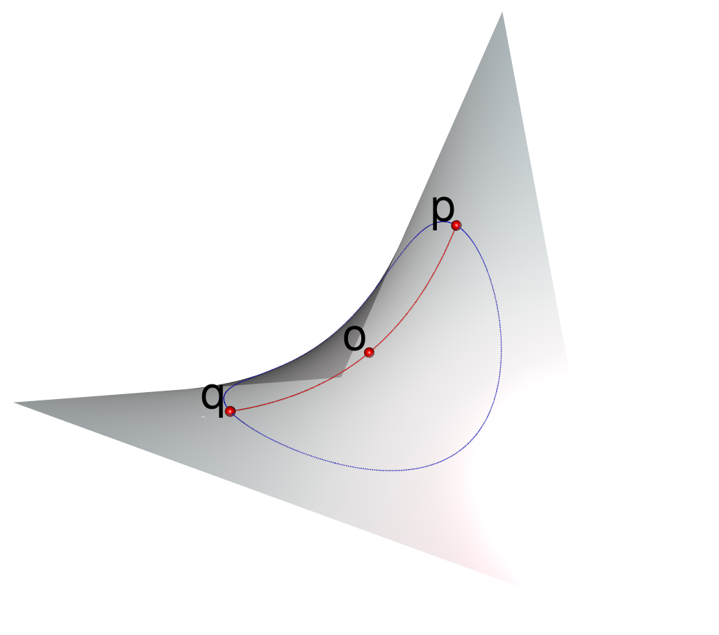
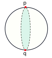
Figure 1: Left Panel: Representation of a geodesic ball of diameter $\overline{PQ}$ and center $O$ on a hyperbolic paraboloid. Right Panel: A graph of two minimizing geodesics that join two antipodal points of a sphere.

Let $(\mbox{$\mathcal{M}$},g)$ be a connected and orientable Riemannian manifold,(see [22], page $18$). We will assume that $(\mbox{$\mathcal{M}$},d_{g})$ is a complete separable metric space. Since $(\mbox{$\mathcal{M}$},d_{g})$ is complete, the Hopf–Rinow theorem (see [22], p.146) implies that for any pair of points $p,q\in\mbox{$\mathcal{M}$}$ there exist at least one geodesic path in $\mathcal{M}$ connecting $p$ and $q$. If the manifold $\mathcal{M}$ fulfills the assumptions of the Cartan–Hadamard Theorem (see [23], p.162)–that is, if $\mathcal{M}$ is a simply connected, complete Riemannian manifold with non–positive curvature (a Hadamard manifold), then the geodesic is unique. Let $X$ be a random element taking values in $\mathcal{M}$, with distribution $P$. In many useful examples (eg. the sphere), it occurs that geodesic uniqueness fails. But in what follows, we will only need that this failure not occurs too often. Roughly speaking, we will assume a condition on $P$ ensuring that there is a unique geodesic between each pair of points $p,q\in\mbox{$\mathcal{M}$}$ with probability one. More precisely, we will assume that the random element $Y$ has a density $f_{Y}$ with respect to the volume measure $d\nu(y)$ on $\mathcal{M}$, (which exists since $\mathcal{M}$ is orientable - see the last section of [24]) fulfilling the following condition: Given $q\in\mbox{$\mathcal{M}$}$ let

$$A_{q}\mathrel{\mathop{:}}=\left\{y\in\mbox{$\mathcal{M}$}\Big{/}\begin{array}[]{ll}\textrm{ there are more than one different }\\ \textrm{minimizing geodesic connecting $y$ and $q$}\end{array}\right\}.$$ (2.1)

Then, there exist a Borel set $B_{q}\subset\mbox{$\mathcal{M}$}$ with $A_{q}\subset B_{q}$ and such that for any $q\in\mbox{$\mathcal{M}$}$

$$\int_{B_{q}}f_{Y}(y)d\nu(y)=0.$$ (2.2)

Remark 1.

Let $C_{\mbox{$\mathcal{M}$}}(p)$ stand for the cut locus of $p$ in a complete manifold $\mathcal{M}$, (see [22], p. $267$). If $P\left(Y\in C_{\mbox{$\mathcal{M}$}}(p)\right)=0$, for all $p\in\mbox{$\mathcal{M}$}$, then condition (2.2) is fulfilled (see [25]). For instance, if the Riemannian manifold is Hadamard, then the cut locus of any point $p$ is empty and the condition is obviously fulfilled. In the unit sphere $S_{d}\mathrel{\mathop{:}}=\{u\in\mathbb{R}^{d}/\|u\|=1\}$ the cut locus of a point $p$ is its opposite point $-p$ and any probability measure having a density supported by the sphere fulfills condition (2.2).

In this paper, we will assume that the Riemannian manifold $(\mbox{$\mathcal{M}$},g)$ with the induced distance $d_{g}$ is connected and oriented, and that the metric space $(\mbox{$\mathcal{M}$},d_{g})$ is separable and complete. We will also assume that given two points $p,q\in\mbox{$\mathcal{M}$}$ there is a unique geodesic determined by $p,q$ with probability one with respect to the tensorial probability measure $d\xi(p,q)\mathrel{\mathop{:}}=f_{Y}(p)f_{Y}(q)d\nu(p)d\nu(q)$, (see Figure 2).

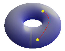
Figure 2: Left Panel: A graph of a geodesic that determines two points on the representation of a face. Right Panel: A graph of a geodesic that determines two points on the representation of a Torus.

2.1 Geodesic balls with diameter $\overline{pq}$

For any pair $p,q\in\mbox{$\mathcal{M}$}$ that determine a unique geodesic $\overline{pq}$, we define the ball of diameter $\overline{pq}$ as the closed ball whose center is the middle point of the geodesic joining $p$ and $q$ with radius $d_{g}(p,q)/2$. It will be denoted by $B_{pq}$. Figure 1 depicts a geodesic ball of diameter $p$ and $q$, where $o$ is the midpoint of the geodesic. In [26] it is shown that the family $\mathcal{B}_{p}:=\{{B}_{p},p\in\mbox{$\mathcal{M}$}\}$ of geodesic balls with center $p$ is a determining class; that is, if two probability measures $\eta,\nu$ on $\mathcal{M}$ coincide on any event of this class, then $\eta=\nu$. We assume that $\mathcal{M}$ is a compact Riemannian manifold. We will start by proving that the family of balls

$$\mathcal{B}_{pq}:=\{B_{pq},p,q\in\mbox{$\mathcal{M}$}\ \textrm{and there is a unique geodesic between $p$ and $q$}\}$$

is also a determining class if the radius of injectivity $r_{iny}$ of $\mathcal{M}$ is positive. We will need the following weaker assumption:

HB) B-continuity A probability measure $\nu$ defined on a Riemannian manifold $\mathcal{M}$ fulfils HB if $\nu(\partial A)=0$ for all closed Borel sets $A$ on $\mathcal{M}$ (Here $\partial A$ denotes the topological boundary of the set $A$).

Property 1.

Let $(\mbox{$\mathcal{M}$},g)$ be a compact Riemannian manifold and $\nu$ be a probability distribution fulfilling HB, such that $\nu\left(\partial\mbox{$\mathcal{M}$}\right)=0$. If the injectivity radius is positive then $\mathcal{B}_{pq}$ is a determining class of $\nu$.

In [27] we showed what if $K\in\mbox{$\mathcal{M}$}$ is a compact set, then the family of balls $\mathcal{B}_{pq}$ is also a Glivenko–Cantelli class in $K$; that is,

$$\sup_{p,q\in K}|P\left(B_{pq}\right)-P_{n}\left(B_{pq}\right)|\rightarrow 0\quad\textrm{a.s. \ \ as $n\rightarrow+\infty$}.$$

In the next section, we define a sensitivity index using this family of sets.

3 Sensitivity Index in Geodesic Balls

In order to build a sensitivity index, we use an idea previously developed in [14]. In our frame we compare the distribution $P_{Y}$ and the conditional distribution $P_{Y|X_{i}}$ on the family of geodesic balls on the manifold (instead of half–lines in [14]. So that, we build an intrinsic index related to the manifold. This index depends only on the dimension and structure of the manifold and not on the dimension of the space where it is immersed, unlike in [6] and [14].

3.1 Constructing the index

Let $\mathbb{X}=(X_{1},\ldots,X_{d})\in\mbox{$\mathbb{R}$}^{d}$ be an random vector and assume that $\mathbb{P}\mathrel{\mathop{:}}=\mathbb{P}_{1}\times\ldots\times\mathbb{P}_{d}$ is the probability law of $\mathbb{X}$. Further, let

$$Z=f(X_{1},\ldots,X_{d}),$$

where $f:\mathbb{R}^{d}\rightarrow\mbox{$\mathcal{M}$}$ is a continuous function. Here, $\mathcal{M}$ a Riemannian manifold of dimension $k$. We wish to understand how sensitive is the output $Z$ to perturbations in some of the input variables $(X_{1},\ldots,X_{d})$. As any manifold can be immersed in $\mathbb{R}^{p}$ for a sufficiently large $p$ (see [28]), this problem could be considered as a particular case of a multivariate output. Nevertheless, in such a way the geometry and “minor dimensionality” of the output are not taken into account. We begin by studying a very particular case and then extend our results to any Riemannian manifold, that satisfies the previous conditions. Let $h$ a measurable function such that $h(X_{1},X_{2})$ is integrable, we set

$$\mbox{$\mathbb{E}$}_{X_{2}}\left(h(X_{1},X_{2})\right)\mathrel{\mathop{:}}=\mbox{$\mathbb{E}$}\left(h(X_{1},X_{2})/X_{1}\right).$$

3.2 A very particular case: The real line.

Let us first focus on the very particular case $\mbox{$\mathcal{M}$}=\mbox{$\mathbb{R}$}$. Let $F$ be the distribution function of $Z$, $F(t)\mathrel{\mathop{:}}=P(Z\leq t)\,(t\in\mathbb{R})$, and $F^{\nu}$ be the distribution of $Z$ conditioned by a subset of the variable $(X_{1},\ldots,X_{d})$. That is, let $\nu=\{i_{1},\ldots,i_{k}\}\subset\{1,\dots,d\}$, and

$$X_{\nu}\mathrel{\mathop{:}}=(X_{i_{1}},\ldots,X_{i_{k}}),$$

$$F^{\nu}(t)\mathrel{\mathop{:}}=\mbox{$\mathbb{E}$}\left(\mathbbm{1}_{(\infty,t]}(Z)\big{|}X_{\nu}\right).$$

In [14] the following Cramér von Mises sensitivity index is considered. Assume that $F$ is absolutely continuous. This normalized index (denoted by $C^{\nu}_{2}$) is defined as

$$C^{\nu}_{2}\mathrel{\mathop{:}}=\frac{N^{\nu}_{2,}}{\int_{\mathbb{R}}F(x)\left(1-F(x)\right)dF(x)}=6N^{\nu}_{2},$$ (3.1)

where

$$N^{\nu}_{2}=\int\mbox{$\mathbb{E}$}\left(\left[F(t)-F^{\nu}(t)\right]^{2}\right)dF(t)$$

$$=\int\left(\mbox{$\mathbb{E}$}\left[\int\mathbbm{1}_{(\infty,t]}(z)d(F-F^{\nu})(z)\right]^{2}\right)dF(t)$$

$$=\mbox{$\mathbb{E}$}\left\{\mbox{$\mathbb{E}$}\left(\left[\mbox{$\mathbb{E}$}\left(\mathbbm{1}_{(\infty,t]}(Z)\right)-\mbox{$\mathbb{E}$}\left(\mathbbm{1}_{(\infty,t]}(Z)\big{|}X_{\nu}\right)\right]^{2}\right)\right\}.$$

To build of our new index, we replace the function $\mathbbm{1}_{(\infty,t]}$ by the indicator function of the interval $[\min(s,t),\max(s,t)]$ (denoted by $h_{s,t}$),

$$h_{s,t}(x)\mathrel{\mathop{:}}=\mathbbm{1}_{\{s\leq x\leq t\}}+\mathbbm{1}_{\{t\leq x\leq s\}}=\mathbbm{1}_{\{\min\{s,t\}\leq x\leq\max\{s,t\}\}}.$$

The function $h_{s,t}$, can be thought of as the indicator function of the ball of diameter $\overline{st}$ in $\mathbb{R}$. Further, let

$$H(s,t)\mathrel{\mathop{:}}=\mbox{$\mathbb{E}$}\left[h_{s,t}(Z)\right]\quad\textrm{and}\quad H^{\nu}(s,t)=\mbox{$\mathbb{E}$}\left[h_{s,t}(Z)\Big{|}X_{\nu}\right].$$ (3.2)

Obviously, $\mbox{$\mathbb{E}$}_{X_{\nu}}\left[H^{\nu}(s,t)\right]=H(s,t)$.

Definition 3.1.

The normalized ball sensitivity index (denoted by $B^{\nu}_{2}$) is then defined as,

$$B^{\nu}_{2}\mathrel{\mathop{:}}=\frac{S^{\nu}_{2}}{\int_{\mathbb{R}^{2}}H(x,y)\left(1-H(x,y)\right)dF(y)dF(x)}=6S^{\nu}_{2},$$ (3.3)

where

$$S^{\nu}_{2}\mathrel{\mathop{:}}=\mbox{$\mathbb{E}$}_{Z_{1},Z_{2}}\left[\mbox{$\mathbb{E}$}_{X_{\nu}}\left\{\left[H(Z_{1},Z_{2})-H^{\nu}(Z_{1},Z_{2})\right]^{2}\right\}\right],$$ (3.4)

and $Z_{1}$ and $Z_{2}$ are two independent copies of $Z$. (The constant 6 follows from the well known fact that $\int_{t>s}(t-s)(1-(t-s))dtds=\int_{t\leq s}(t-s)(1-(t-s))dtds=1/12$.)

We may can rewrite $S^{\nu}_{2}$ as

$$S^{\nu}_{2}=\int_{\mbox{$\mathcal{M}$}\times\mbox{$\mathcal{M}$}}\mbox{$\mathbb{E}$}_{X_{\nu}}\left\{\left(H(z_{1},z_{2})-H^{\nu}(z_{1},z_{2})\right)^{2}\right\}dF(z_{1})dF(z_{2}).$$

3.3 Generalization for a Riemannian manifold

As discussed before, $\mathcal{M}$ is a Riemannian manifold of dimension $k$. So that, under some regularity conditions, given two points $\{z_{1},z_{2}\}\subset\mbox{$\mathcal{M}$}$, the following function $h_{z_{1},z_{2}}:\mbox{$\mathcal{M}$}\rightarrow\{0,1\}$ is generically well defined,

$$h_{z_{1},z_{2}}(t)\mathrel{\mathop{:}}=\mathbbm{1}_{B_{z_{1}z_{2}}}(t).$$

Let $Z_{1},Z_{2}$ be independent copies of $Z$. Our normalized sensitivity index is built by means of balls as in Definition 3.1,

$$B^{\nu}_{2}\mathrel{\mathop{:}}=\frac{S^{\nu}_{2}}{D^{\nu}_{2}},$$ (3.5)

where

$$S^{\nu}_{2}\mathrel{\mathop{:}}=\mbox{$\mathbb{E}$}_{Z_{1},Z_{2}}\left[\mbox{Var}_{X_{\nu}}\left\{\mbox{$\mathbb{E}$}_{Z}\left[h_{Z_{1},Z_{2}}(Z)\Big{|}X_{\nu}\right]\right\}\right],$$

and

$$D^{\nu}_{2}\mathrel{\mathop{:}}=\mbox{$\mathbb{E}$}\left[H(Z_{1},Z_{2})\left(1-H(Z_{1},Z_{2})\right)\right].$$

Notice that the index defined in the previous subsection is a particular case with $\mbox{$\mathcal{M}$}=\mbox{$\mathbb{R}$}$.

Remark 2.

If $B^{\nu}_{2}=0$ we have that $\mbox{$\mathbb{E}$}_{Z}\left[h_{z_{1},z_{2}}(Z)\Big{|}X_{\nu}\right]=\mbox{$\mathbb{E}$}_{Z}\left[h_{z_{1},z_{2}}(Z)\right]\,a.s.$ for all $(z_{1},z_{2})\in\Omega\subset\mathcal{M}\times\mathcal{M}$ with $P(\Omega)=1$. Therefore, under the assumptions of Property 1, the probability measures $P_{Z|X_{\nu}}$ and $P_{Z}$ are the same.

3.4 Estimation

In the next subsection, an estimator of the index $B^{\nu}_{2}$ is proposed. The variance of the conditional mean is estimated using the pick and freeze method (see [3] and [29]). Further, as the expected value $\mbox{$\mathbb{E}$}_{Z_{1},Z_{2}}(\cdot)$ is a symmetric function of $Z_{1}$ and $Z_{2}$ we will use an $U$–statistic. At the end of the next subsection, the steps for the construction of the estimator will be detailed.

3.4.1 Estimation by “Pick and Freeze” method

The method consists in writing the variance of the conditional mean as a covariance. For $\nu\in\{1,\ldots,d\}$, let $X^{\nu}$ be the random vector that coincides with $X$ on its $\nu$ components and is independently regenerated on the others components. That is, $X^{\nu}_{\nu}=X_{\nu}$ and $X^{\nu}_{\bar{\nu}}=X^{{}^{\prime}}_{\bar{\nu}}$, where $X^{{}^{\prime}}$ is an independent copy of $X$ and $\bar{\nu}$ is the complementary set of $\nu$ ($\bar{\nu}=\{1,\ldots,d\}\setminus\nu$). We set

$$Z^{\nu}\mathrel{\mathop{:}}=f(X^{\nu}).$$

For sake of simplicity assume first that $\mbox{$\mathbb{E}$}(Z)=0$. Then,

$$\mbox{Var}\left(\mbox{$\mathbb{E}$}(Z\big{|}X_{\nu})\right)=\mbox{$\mathbb{E}$}\left(\mbox{$\mathbb{E}$}^{2}(Z\big{|}X_{\nu})\right).$$ (3.6)

Since $Z$ and $Z^{\nu}$ are conditionally independent of $X_{\nu}$ (see [30]), so that

$$\mbox{cov}(Z,Z^{\nu})=\mbox{$\mathbb{E}$}(ZZ^{\nu})-\mbox{$\mathbb{E}$}(Z)\mbox{$\mathbb{E}$}(Z^{\nu})=\mbox{$\mathbb{E}$}(ZZ^{\nu})-\mbox{$\mathbb{E}$}^{2}(Z)$$

$$=\mbox{$\mathbb{E}$}\left[\mbox{$\mathbb{E}$}(ZZ^{\nu}\big{|}X_{\nu})\right]=\mbox{$\mathbb{E}$}\left[\mbox{$\mathbb{E}$}(Z\big{|}X_{\nu})\mbox{$\mathbb{E}$}(Z^{\nu}\big{|}X_{\nu})\right]$$

$$=\mbox{$\mathbb{E}$}\left[\mbox{$\mathbb{E}$}^{2}(Z|X_{\nu})\right].$$

Following [30], estimating the covariance by a Monte Carlo Method we obtain the following Pick Freeze estimator of $\mbox{Var}\left[\mbox{$\mathbb{E}$}(Z|X_{\nu})\right]$,

$$T^{\nu}\mathrel{\mathop{:}}=\frac{1}{N}\sum_{j=1}^{N}Z_{j}Z_{j}^{\nu}-\left(\frac{1}{2N}\sum_{j=1}^{N}(Z_{j}+Z_{j}^{\nu})\right)^{2}.$$ (3.7)

Here, $Z_{j}$ and $Z^{\nu}_{j}$, are $N$ independent copies of $Z$ and $Z^{\nu}$ respectively.

First step. Using the previous idea, we build a consistent estimator of the numerator $S^{\nu}_{2}$. Let $\mathcal{P}_{N,p}$ be the set of all possible subsets of $\{1,\ldots,N\}$ with $p$ elements, that is,

$$\mathcal{P}_{N,p}=\{(i_{1},\ldots,i_{p})\in\{1,\ldots,N\}^{p}/i_{1}<\ldots<i_{p}\}.$$

Let $\tau=(i_{1},\ldots,i_{p})\in\mathcal{P}_{N,p}$. We denote by $\textbf{W}_{\tau}=\left(W_{i_{1}},\ldots,W_{i_{p}}\right)$ a sample of $p$ independent copy of $Z$. The estimator is obtained as follows,

Further, $D^{\nu}_{2}$ is estimated analogously setting

$$\hat{D}^{\nu}_{2}\mathrel{\mathop{:}}=\frac{1}{\binom{N}{2}}\sum_{\tau\in\mathcal{P}_{N,2}}\Big{\{}\frac{1}{2N}\sum_{j=1}^{N}\left(h_{\textbf{W}_{\tau}}\left(Z_{j}\right)+h_{\textbf{W}_{\tau}}\left(Z_{j}^{\nu}\right)\right)-$$

$$-\left(\frac{1}{2N}\sum_{i=1}^{N}\left[h_{\textbf{W}_{\tau}}\left(Z_{i}\right)+h_{\textbf{W}_{\tau}}\left(Z_{i}^{\nu}\right)\right]\right)^{2}\Big{\}}.$$

The computation of the estimator is simple. Indeed, it only involves computation of indicator functions. Nevertheless, the computational time to perform this estimator could be high. Indeed, the number of sums is of order $N^{3}$. Each term involves the determination of a geodesic. In the following section, we give some asymptotic properties of this estimator. We provide an exponential inequality that leads, from the Borel–Cantelli Lemma, to strong consistency.

3.5 Asymptotic properties of $\hat{B}^{\nu}_{2}$.

We analyzed separately the strong convergence of $\hat{S}^{\nu}_{2}$ and $\hat{D}^{\nu}_{2}$. The strong convergence of $\hat{S}^{\nu}_{2}$ follows from the next Theorem. Notice that another proof may be built using the fourth moment and the Rosenthal inequality for $U$–statistic of order $2$ developed in [31].

Theorem (Exponential inequality ) Let $s>0$, there exist $N_{0}$ such that if $N>N_{0}$,

$$P\left(\left|\hat{S}^{\nu}_{2}-S^{\nu}_{2}\right|>s\right)\leq 16\exp\left\{-\frac{N\left(\frac{s}{9}\right)^{2}}{8}\right\}.$$ (3.8)

From the previous Theorem and the Borel–Cantelli Lemma the strong consistency of $\hat{S}^{\nu}_{2}$ follows.

Corollary (Consistency of the estimator) $\hat{S}^{\nu}_{2}$ is a consistent estimator of $S^{\nu}_{2}$.

Notice that we may analogously show the convergence of the denominator involved in (3.5).

4 Simulations

This simulation section is made up on three examples. The first one shows the accuracy of the estimator when the output is real valued. In the second example the output lies on a circle immersed in $\mathbb{R}^{2}$. The estimates are compared with those obtained in [14]. The last example shows that the index proposed in [14] may fail as sensitivity indicator.

4.1 Example 1: Output on the real line

We study here an example where the Sobol index does not provide information on sensitivity, while $D^{\nu}_{2}$ and $B^{\nu}_{2}$ do. Let $Z=\alpha X_{1}+X_{2}$ where $\alpha>0$, and $X_{1},X_{2}$ are independent. Assume further that $X_{1}\sim\textrm{Bernoulli}(p)$, $X_{2}\sim F$, with $m=\mbox{$\mathbb{E}$}(X_{2})$, $\sigma^{2}=\textrm{Var}(X_{2})=\alpha^{2}p(1-p)$.

We calculate $B^{1}_{2}$ in the Appendix while $C^{1}_{2}$ has been calculated in [14]. In the case when $X_{2}\sim U(0,b)$ with $b=\sqrt{12\alpha^{2}p(1-p)}$. We find

$$B^{1}_{2}=12p(1-p)\begin{cases}\left(\frac{\alpha}{b}\right)^{3}\left(\frac{1}{3}-\frac{1}{4}\frac{\alpha}{b}\right)&\text{if }\alpha\leq b,\\ 1/12&\text{if }\alpha>b,\end{cases}$$

$$C^{1}_{2}=6p(1-p)\begin{cases}\left(\frac{\alpha}{b}\right)^{2}\left(1-\frac{2}{3}\frac{\alpha}{b}\right)&\text{if }\alpha\leq b,\\ 1/3&\text{if }\alpha>b,\end{cases}$$

In the Figure 3, the estimates of both indices are compared for different values of $p\in[0,1]$. Samples sizes $100$, $500$ and $1000$ are considered. For each $p$, through resampling Bootstrap for $U$–statistics (see [32]), $95\%$ confidence intervals are also given. In all cases, the mean squared deviation (MSD) of the estimators are computed. The MSD of $\hat{B}^{1}_{2}$ is slightly smaller than the one for $\hat{C}^{1}_{2}$ (see Table 1). Similar results are obtained when comparing $\hat{B}^{2}_{2}$ and $\hat{C}^{2}_{2}$.

Size	$MSD_{\hat{B}^{1}_{2}}$	$MSD_{\hat{C}^{1}_{2}}$
$N=100$	0.051	0.067
$N=500$	0.022	0.028
$N=1000$	0.013	0.018

Table 1: The MSD of the $\hat{B}^{1}_{2}$ and $\hat{C}^{1}_{2}$ estimators for sample sizes $N=100,500$ and $1000$.

We may conclude that the new proposed index has a similar behavior as the Cramér von Mises one for the real line.

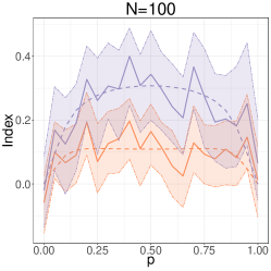
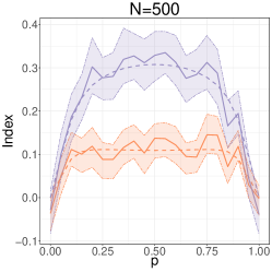
Figure 3: Cramér von Mises indexes and our new indexes for Example 4.1. In all cases, ($\textendash\,\,\textendash$) are the true index and ($\mathrel{-}\joinrel\mathrel{-}$) their estimate. Violet color depicts CVM sensitivity index while orange color depicts Ball sensitivity index. The $95\%$ bootstrap confidence intervals are represented with shading. Left–hand Panel: $N=100$. Center–hand Panel: $N=500$. Right–hand Panel: $N=1000$.

4.2 Example 2: Output on a simple manifold immersed in $\mathbb{R}^{2}$

The case where $Z$ ranges on the unit circle $S_{1}$ of $\mathbb{R}^{2}$ is considered. We assume that the input vector has distribution

$$X=\binom{X_{1}}{X_{2}}\sim N\left[\binom{\mu_{1}}{\mu_{2}},\left(\begin{array}[]{cc}\sigma^{2}_{1}&0\\ 0&\sigma^{2}_{2}\end{array}\right)\right].$$

Here, we study the case when the output $Z$ is the normalized version of $X$

$$Z\mathrel{\mathop{:}}=\frac{X}{\|X\|}.$$

The distribution of $Z$ has been widely studied, we refer for example to [16], [33] and [34]. In Figure 4 the index proposed in [14] and the one studied here are depicted for the last system. These sensitivity indices are computed for $\mu_{1}\in[-5,0]$. The other values are setted to $\mu_{2}=0$ and $\sigma^{2}_{1}=\sigma^{2}_{2}=1$. We observe that the variability of $\hat{B}^{\nu}_{2}$ is smaller that the one of $\hat{D}^{\nu}_{2}$ for a sample size $N=300$.

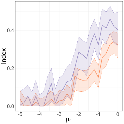
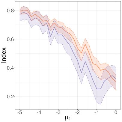
Figure 4: Calculation of the indices $\hat{B}^{\nu}_{2}$ and $D^{\nu}_{2}$ in the equation 4.2 with $\mu_{1}\in[-5,0]$ and $N=300$. For all cases, it is represented using ($\mathrel{-}\joinrel\mathrel{-}$) the index estimation functions for $N=300$. In violet color depicts CVM sensitivity index and orange color depicts Ball sensitivity index. The $95\%$ bootstrap confidence intervals are represented with shading. Left–hand Panel: $\nu=1$. Right–hand Panel: $\nu=2$.

4.3 Example 3: Output on a manifold immersed in $\mathbb{R}^{3}$

Let us now consider a system with output in the following manifold $\mathcal{M}$ immersed in $\mathbb{R}^{3}$

$$\mbox{$\mathcal{M}$}=\left\{(x,y,z)\in\mathbb{R}^{3}/xyz=1,\,\,x,y,z>0\right\}.$$

More precisely, let $Z=f(X,Y)\mathrel{\mathop{:}}=(X+Y,\frac{1}{X},\frac{X}{X+Y})$ where $X$ and $Y$ are iid random variables with Gamma distribution with parameters $(\mu_{1},1)$, $(\mu_{1}>0)$. Since the function $\mathbbm{1}_{\{z\leq w\}}=0$ for all $z,w\in M,z\neq w$, the index estimation $\hat{C}^{\nu}_{2}$ based on the left lower quadrants introduced in [14], does not provide any information about the sensitivity. Also the second moment of $1/X$ does not exist, therefore it is not possible to compute the Sobol’ index defined in [6]. By varying the parameter $\mu_{1}$, we calculate the estimation of the ball sensitivity index $B^{1}_{2}$ and $B^{2}_{2}$ . For this purpose, $N=1000$ pick-freeze samples were generated for each value of $Z$, $(Z_{j},Z^{\nu}_{j})$, $j=1,\ldots,N$; and other $1000$ samples of $Z$, independent of $(Z_{j},Z^{\nu}_{j})$ for the corresponding $W_{k}$. In Figure 5 the values of the indices are observed by varying the parameter $\mu_{1}$ between $0$ and $5$. It is clear from Figure 5 that the new index is able to detect the effect of each variable on the output for different values of the parameter $\mu$.

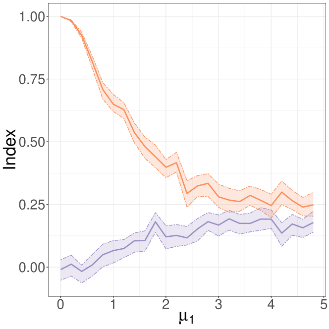
Figure 5: Calculation of the index $\hat{B}^{\nu}_{2}$

5 Sensitivity for isotropic matrix

We consider now the stiffness matrix $Z$ of an isotropic materials as a function of the constants of Lamé $\lambda$ and $\mu$ (see [35], p. 13). Hence, if the temperature is constant we have

$$Z=\left(\begin{array}[]{cccccc}K+4\mu/3&K-2\mu/3&K-2\mu/3&0&0&0\\ K-2\mu/3&K+4\mu/3&K-2\mu/3&0&0&0\\ K-2\mu/3&K-2\mu/3&K+4\mu/3&0&0&0\\ 0&0&0&\mu&0&0\\ 0&0&0&0&\mu&0\\ 0&0&0&0&0&\mu\\ \end{array}\right)$$

where $K=\lambda+2\mu/3$ is the volumetric modulus. The parameter $\mu$ is called the stiffness modulus, $K$ and $\mu$ take nonnegative values and are are modeled with a distribution supported by $\mathbb{R}^{+}$. The set of stiffness matrices is considered as a sub–manifold of the Riemannian manifold of the symmetric positive-definite matrices with the metric $g$. This manifold is usually denoted by $(\mathbb{P}_{d},g)$, we refer to [36] for more on the subject. Given two matrices $A$ and $B$ there exists an unique geodesic joining $A$ and $B$ given by,

$$\gamma(t)\mathrel{\mathop{:}}=A^{1/2}\left(A^{-1/2}BA^{-1/2}\right)^{t}A^{1/2}.$$ (5.1)

So that, we can calculate the midpoint between $A$ and $B$. We will denote by $A\#B$ this midpoint. We have

$$A\#B=A^{1/2}\left(A^{-1/2}BA^{-1/2}\right)^{1/2}A^{1/2}$$ (5.2)

$$d(A,B)=\|\textrm{ln}\left(A^{-1/2}BA^{-1/2}\right)\|,$$ (5.3)

where $\|\cdot\|$ is the Hilbert–Schmidt norm. Note that the midpoint is simply the geometric mean of the matrices.

We will focus on the case when $K$ and $\mu$ are independent random variables and on two scenarios:

Case 1	$\quad K\sim\gamma(1/\lambda_{K},\lambda_{K})$	$\mu\sim\gamma(1/\lambda_{\mu},\lambda_{\mu})$
Case 2	$\quad K\sim\textrm{U}(1-\lambda_{K},1+\lambda_{K})$	$\mu\sim\textrm{U}(1-\lambda_{\mu},1+\lambda_{\mu})$

Tables 2 and 3 show the values of $\hat{B}^{1}_{2}$ and $\hat{B}^{2}_{2}$ for various values of $(\lambda_{K},\lambda_{\mu})$. The sample size was $N=500$. In both tables we can see that the new index provides significant information regarding the sensibility of $Z$ with respect to the input variables $K$ and $\mu$. In particular, when the variance of the input variables increases (larger $\lambda_{\mu}$ or $\lambda_{K}$) the value of the index increases, i.e. a a greater effect is observed on the output.

Table 2: Index on isotropic matrix with Gamma distributions parameter

Distribution	Case 1: $B^{1}$				Case 1: $B^{2}$
$\lambda_{\mu}\Big{\backslash}\lambda_{K}$	0.001	0.01	0.1	1	0.001	0.01	0.1	1
0.001	0.625	0.212	0.016	0.001	0.083	0.435	0.855	0.980
0.01	0.925	0.593	0.215	0.033	0.004	0.072	0.458	0.865
0.1	0.987	0.912	0.587	0.184	0.001	0.006	0.137	0.518
1	0.999	0.990	0.930	0.600	0.000	0.007	0.210	0.311

Table 3: Index on isotropic matrix with Uniform distributions parameter

Distribution	Case 1: $B^{1}$				Case 1: $B^{2}$
$\lambda_{\mu}\Big{\backslash}\lambda_{K}$	0.001	0.01	0.1	1	0.001	0.01	0.1	1
0.001	0.620	0.008	0.001	0.000	0.109	0.848	0.997	1.000
0.01	0.989	0.623	0.003	0.001	0.018	0.092	0.849	0.997
0.1	1.000	0.989	0.623	0.624	0.016	0.016	0.102	0.846
1	1.000	1.000	0.990	0.987	0.015	0.016	0.100	0.211

6 Conclusions and Future Work

We introduce a new framework to measure the global sensitivity for system outputs valued on a Riemannian manifolds. This sensitivity index has nice properties:

1. It is a generalization of the one proposed by [14].

2. It is built on the whole distributions and not only on moments.

3. The construction of the index lies on the geometry of the support of the output through the geodesic distance.

4. A pick-freeze like estimator of the index based on an $U$–statistic is proposed. It is easy to compute. The consistency of the estimator is shown.

5. Considering various simulation scenarios, the desirable properties of the estimator are illustrated. Using a Bootstrap resampling method for $U$–statistics we construct confidence intervals.

6. The sensitivity index for an isotropic matrix model is studied.

7. In future research we will challenge to study new applications, for instance, the impact of inputs generated by a dynamic system, when the output is supported by a Riemannian Lie Group.

Appendix

1. Proof of Property 1.

   In [26] it is shown that both the sets

   $$\mathcal{B}\mathrel{\mathop{:}}=\{{B}_{p,r}\big{/}p\in\mbox{$\mathcal{M}$}\,\textrm{and}\,r>0\},\ \mbox{and}\ \mathcal{B}_{\delta}\mathrel{\mathop{:}}=\{{B}_{p,r}\big{/}p\in\mbox{$\mathcal{M}$}\,\textrm{and}\,0<r<\delta\},$$ (6.1)

   are determining classes. We aim to show that the family of balls

   $$\mathcal{B}_{pq}:=\{B_{pq},p,q\in\mbox{$\mathcal{M}$}\ \textrm{and there is a unique geodesic between $p$ and $q$}\},$$

   is also a determining class if the radius of injectivity $r_{iny}$ of $\mathcal{M}$ is positive. Recall that in a metric space the family of closed sets $\mathcal{C}$ is a determining class ([37], page $7$). Therefore, it suffices to show that if two probabilities $\nu$ and $\eta$ coincides on $\mathcal{B}_{pq}$, then $\nu(A)=\eta(A)$ for all $A\in\mathcal{C}$. Let $\partial A$ the topological boundary of $A$ and $\partial A^{\epsilon}\mathrel{\mathop{:}}=\bigcup_{x\in\partial A}B(x,\epsilon)$ for $\epsilon>0$. So,

   $$\nu(A)=\nu\left(A\setminus(\partial A^{\epsilon}\cup\partial\mbox{$\mathcal{M}$}^{\epsilon})\right)+\nu\left(A\cap(\partial A^{\epsilon}\cup\partial\mbox{$\mathcal{M}$}^{\epsilon})\right).$$

   Let $\epsilon^{*}\mathrel{\mathop{:}}=\min(\epsilon/2,r_{iny})$. Since by (6.1) $\mathcal{B}_{\epsilon^{*}}$ is a determining class, using the exponential map we derive that the set of balls in $\mathcal{B}_{\epsilon^{*}}$ that determine the $\nu$-probability of $A\setminus(\partial A^{\epsilon^{*}}\cup\partial\mbox{$\mathcal{M}$}^{\epsilon^{*}})$ are in $\mathcal{B}_{pq}$. Therefore,

   $$\nu\left(A\setminus(\partial A^{\epsilon^{*}}\cup\partial\mbox{$\mathcal{M}$}^{\epsilon^{*}})\right)=\eta\left(A\setminus(\partial A^{\epsilon^{*}}\cup\partial\mbox{$\mathcal{M}$}^{\epsilon^{*}})\right).$$

   Finally, from the dominated convergence theorem and the assumptions, we conclude that

   $$\nu(A)=\eta(A)-\eta(\partial A\cup\partial\mbox{$\mathcal{M}$})+\nu(\partial A\cup\partial\mbox{$\mathcal{M}$})=\eta(A).$$

   $\square$

2. Proof of Property 3.5.

   We will show that given $s>0$, there is an $N_{0}$ such that for any $N>N_{0}$,

   $$P\left(\left|\hat{S}^{\nu}_{2}-S^{\nu}_{2}\right|>9s\right)\leq 16\exp\left\{-\frac{N^{2}}{8}\right\}.$$ (6.2)

   We will prove that

   $$P\left(\hat{S}^{\nu}_{2}-S^{\nu}_{2}>9s\right)\leq 8\exp\left\{-\frac{Ns^{2}}{8}\right\},$$

   and it is analogous for the other tail.

   For $1\leq j,k\leq N$ and $\tau\in\mathcal{P}_{N,2}$ let,

   • $\textbf{W}_{\tau}=\left(W_{k_{1}},W_{k_{2}}\right)$

   • $\textbf{Z}_{j}=\left(Z_{j},Z_{j}^{\nu}\right)$

   • $G(\textbf{Z}_{j},\textbf{W}_{\tau})=h_{\textbf{W}_{\tau}}(Z_{j})h_{\textbf{W}_{\tau}}(Z_{j}^{\nu})$

   • $J(\textbf{Z}_{j},\textbf{W}_{\tau})=\frac{1}{2}\left[h_{\textbf{W}_{\tau}}(Z_{j})+h_{\textbf{W}_{\tau}}(Z_{j}^{\nu})\right]$

   • $H(\textbf{Z}_{i},\textbf{Z}_{j},\textbf{W}_{\tau})=J(\textbf{Z}_{i},\textbf{W}_{\tau})J(\textbf{Z}_{j},\textbf{W}_{\tau})$

   The proof is built on three steps:

   • Step 1 [Rewrite the difference $\hat{S}^{\nu}_{2}-S^{\nu}_{2}$] Similarly to [14] but for an $U$–statistics, we have that

     $$\hat{S}^{\nu}_{2}=\frac{1}{N\binom{N}{2}}\sum_{\begin{subarray}{c}j\in\{1,\ldots,N\}\\ \tau\in\mathcal{P}_{N,2}\end{subarray}}G(\textbf{Z}_{j},\textbf{W}_{\tau})-\frac{1}{N^{2}\binom{N}{2}}\sum_{\begin{subarray}{c}\{i,j\}\in\{1,\ldots,N\}\\ \tau\in\mathcal{P}_{N,2}\end{subarray}}H(\textbf{Z}_{i},\textbf{Z}_{j},\textbf{W}_{\tau})$$

     $$=\frac{1}{N\binom{N}{2}}\sum_{\begin{subarray}{c}j\in\{1,\ldots,N\}\\ \tau\in\mathcal{P}_{N,2}\end{subarray}}\left\{G(\textbf{Z}_{j},\textbf{W}_{\tau})-\mbox{$\mathbb{E}$}\left[G(\textbf{Z}_{j},\textbf{W}_{\tau})\right]\right\}-$$

     $$-\frac{1}{N^{2}\binom{N}{2}}\sum_{\begin{subarray}{c}\{i,j\}\in\{1,\ldots,N\}\\ \tau\in\mathcal{P}_{N,2}\end{subarray}}\left\{H(\textbf{Z}_{i},\textbf{Z}_{j},\textbf{W}_{\tau})-\mbox{$\mathbb{E}$}\left[H(\textbf{Z}_{i},\textbf{Z}_{j},\textbf{W}_{\tau})\right]\right\}+$$

     $$+\mbox{$\mathbb{E}$}\left[G(\textbf{Z}_{1},\textbf{W}_{\tau_{1}})\right]-\left(1-\frac{1}{N}\right)\mbox{$\mathbb{E}$}\left[H(\textbf{Z}_{1},\textbf{Z}_{2},\textbf{W}_{\tau_{1}})\right]-\frac{1}{N}\mbox{$\mathbb{E}$}\left[H(\textbf{Z}_{1},\textbf{Z}_{1},\textbf{W}_{\tau_{1}})\right],$$

     and

     $$S^{\nu}_{2}=\mbox{$\mathbb{E}$}_{\textbf{W}_{1}}\left\{\textrm{Var}_{X_{\nu}}\left(H^{\nu}(\textbf{W}_{1})\right)\right\}$$

     $$=\mbox{$\mathbb{E}$}_{\textbf{W}_{1}}\left\{\textrm{Var}_{X_{\nu}}\left(\mbox{$\mathbb{E}$}_{Z}(h_{\textbf{W}_{1}}(Z)/X_{\nu})\right)\right\}=\mbox{$\mathbb{E}$}_{\textbf{W}_{1}}\left\{\textrm{cov}\left(h_{\textbf{W}_{1}}(Z_{1}),h_{\textbf{W}_{1}}(Z_{1}^{\nu})\right)\right\}$$

     $$=\mbox{$\mathbb{E}$}_{\textbf{W}_{1}}\left\{\mbox{$\mathbb{E}$}_{\textbf{Z}_{1}}\left(h_{\textbf{W}_{1}}(Z_{1})h_{\textbf{W}_{1}}(Z_{1}^{\nu})\right)\right\}-\mbox{$\mathbb{E}$}_{\textbf{W}_{1}}\left\{\left[\mbox{$\mathbb{E}$}_{\textbf{Z}_{1}}\left(h_{\textbf{W}_{1}}(Z_{1})\right)\right]^{2}\right\}.$$

     Now, we may decompose the error into three terms

     $$\hat{S}^{\nu}_{2}-S^{\nu}_{2}=\underbrace{\frac{1}{N\binom{N}{2}}\sum_{\begin{subarray}{c}j\in\{1,\ldots,N\}\\ \tau\in\mathcal{P}_{N,2}\end{subarray}}\left\{G(\textbf{Z}_{j},\textbf{W}_{\tau})-\mbox{$\mathbb{E}$}\left[G(\textbf{Z}_{j},\textbf{W}_{\tau})\right]\right\}}_{(A)}-$$

     $$\underbrace{-\frac{1}{N^{2}\binom{N}{2}}\sum_{\begin{subarray}{c}\{i,j\}\in\{1,\ldots,N\}\\ \tau\in\mathcal{P}_{N,2}\end{subarray}}\left\{H(\textbf{Z}_{i},\textbf{Z}_{j},\textbf{W}_{\tau})-\mbox{$\mathbb{E}$}\left[H(\textbf{Z}_{i},\textbf{Z}_{j},\textbf{W}_{\tau})\right]\right\}}_{(B)}+$$

     $$\underbrace{+\frac{1}{N}\left\{\mbox{$\mathbb{E}$}\left[H(\textbf{Z}_{1},\textbf{Z}_{2},\textbf{W}_{\tau_{1}})\right]-\mbox{$\mathbb{E}$}\left[H(\textbf{Z}_{1},\textbf{Z}_{1},\textbf{W}_{\tau_{1}})\right]\right\}.}_{(C)}$$

     In the following steps, we bounded the terms $(A)$ and $(B)$ for a sufficiently large $N$.

     In steps $2$ and $3$ we use Hoeffding inequality (see for example [38]) for independent and real variables. That is, if $W_{1},\ldots,W_{N}$ are independent centred random variables, supported by $[a_{i},b_{i}]\quad i=1,\ldots,N$,

     $$P\left(\sum_{i=1}^{N}W_{i}>s\right)\leq\exp\left\{-\frac{2s^{2}}{\sum_{i=1}^{N}(b_{i}-a_{i})^{2}}\right\}\quad(s>0).$$ (6.3)

     We also use an extension of the previous inequality for $U$–statistics of order $2$, see [39], Theorem A, (5.6). If $s=s(X_{1},X_{2})$ is the $U$–statistics kernel of $U_{n}$ such that $\mbox{$\mathbb{E}$}(s(X_{1},X_{2}))=\theta$ and $a\leq s(x_{1},x_{2})\leq b$. So, for $s>0$ and $N>2$,

     $$P\left(U_{n}-\theta>s\right)\leq\exp\left\{-\frac{Ns^{2}}{(b-a)^{2}}\right\}$$ (6.4)

     For us, the kernels are centred bounded indicator functions.

   • Step 2 [Bounds for $(A)$.]

     Let $G_{c}(\textbf{Z}_{j},\textbf{W}_{\tau})=G(\textbf{Z}_{j},\textbf{W}_{\tau})-\mbox{$\mathbb{E}$}\left[G(\textbf{Z}_{j},\textbf{W}_{\tau})\right]$ and $\tilde{G}(Z_{i},\textbf{W}_{\tau})=G_{c}(Z_{i},\textbf{W}_{\tau})-\mbox{$\mathbb{E}$}_{Z_{i}}(G_{c}(Z_{i},\textbf{W}_{\tau}))$,

     $$A=\underbrace{\frac{1}{N\binom{N}{2}}\sum_{\begin{subarray}{c}i\in\{1,\ldots,N\}\\ \tau\in\mathcal{P}_{N,2}\end{subarray}}\tilde{G}(Z_{i},\textbf{W}_{\tau})}_{A_{1}}+\underbrace{\frac{1}{\binom{N}{2}}\sum_{\tau\in\mathcal{P}_{N,2}}\mbox{$\mathbb{E}$}_{Z}\left[G_{c}(Z,\textbf{W}_{\tau})\right]}_{A_{2}}$$

     $$P(A_{1}>s)=P\left(\frac{1}{N\binom{N}{2}}\sum_{\begin{subarray}{c}i\in\{1,\ldots,N\}\\ \tau\in\mathcal{P}_{N,2}\end{subarray}}\tilde{G}(Z_{i},\textbf{W}_{\tau})>s\right)$$

     $$=P\left(\sum_{i=1}^{N}\frac{1}{\binom{N}{2}}\sum_{\tau\in\mathcal{P}_{N,2}}\tilde{G}(Z_{i},\textbf{W}_{\tau})>Ns\right)$$

     $$\leq\exp\left\{-\frac{s^{2}N}{2}\right\}\leq\exp\left\{-\frac{Ns^{2}}{8}\right\},$$

     while

     $$P(A_{2}>s)=P\left(\frac{1}{\binom{N}{2}}\sum_{\tau\in\mathcal{P}_{N,2}}\mbox{$\mathbb{E}$}_{Z}\left[G_{c}(Z,\textbf{W}_{\tau})\right]>s\right)$$

     $$\leq\exp\left\{\frac{-2Ns^{2}}{8}\right\}\leq\exp\left\{-\frac{Ns^{2}}{8}\right\}.$$

     But, $\left\{A_{1}+A_{2}>2s\right\}\subset\{A_{1}>s\}\cup\{A_{2}>s\}$, so

     $$P(A>2s)\leq 2\exp\left\{-\frac{Ns^{2}}{8}\right\}.$$ (6.5)

   • Step 3 [Bounds for $(B)$.]

     Let $H_{c}(\textbf{Z}_{i},\textbf{Z}_{j},\textbf{W}_{\tau})=H(\textbf{Z}_{i},\textbf{Z}_{j},\textbf{W}_{\tau})-\mbox{$\mathbb{E}$}\left[H(\textbf{Z}_{i},\textbf{Z}_{j},\textbf{W}_{\tau})\right]$ and $\tilde{H}(Z_{i},Z_{j},\textbf{W}_{\tau})=H_{c}(Z_{i},Z_{j},\textbf{W}_{\tau})-\mbox{$\mathbb{E}$}_{Z_{j}}(H_{c}(Z_{i},Z_{j},\textbf{W}_{\tau}))$,

     $$B=\underbrace{\frac{1}{N^{2}\binom{N}{2}}\sum_{\begin{subarray}{c}\{i,j\}\in\{1,\ldots,N\}\\ \tau\in\mathcal{P}_{N,2}\end{subarray}}\tilde{H}(Z_{i},Z_{j},\textbf{W}_{\tau})}_{B_{1}}+$$

     $$+\underbrace{\frac{1}{N\binom{N}{2}}\sum_{\tau\in\mathcal{P}_{N,2}}\mbox{$\mathbb{E}$}_{Z}\left[H_{c}(Z,Z,\textbf{W}_{\tau})\right]}_{B_{2}}+$$

     $$+\underbrace{\frac{N-1}{N^{2}\binom{N}{2}}\sum_{\begin{subarray}{c}j\in\{1,\ldots,N\}\\ \tau\in\mathcal{P}_{N,2}\end{subarray}}\mbox{$\mathbb{E}$}_{Z}\left[H_{c}(Z,Z_{j},\textbf{W}_{\tau})\right]}_{B_{3}}.$$

     We have $\left\{\sum_{i=1}^{3}B_{i}>6s\right\}\subset\{B_{1}>3s\}\cup\{B_{2}>s\}\cup\{B_{3}>2s\}$.

     So that,

     $$P(B_{1}>3s)\leq P\left(\sum_{j}\frac{1}{\binom{N}{2}}\sum_{\tau\in\mathcal{P}_{N,2}}\tilde{H}(Z_{j},Z_{j},\textbf{W}_{\tau})>N^{2}s\right)+$$

     $$+P\left(\sum_{j>i}\frac{1}{\binom{N}{2}}\sum_{\tau\in\mathcal{P}_{N,2}}\tilde{H}(Z_{i},Z_{j},\textbf{W}_{\tau})>N^{2}s\right)+$$

     $$+P\left(\sum_{j<i}\frac{1}{\binom{N}{2}}\sum_{\tau\in\mathcal{P}_{N,2}}\tilde{H}(Z_{i},Z_{j},\textbf{W}_{\tau})>N^{2}s\right)\leq$$

     $$\leq\exp\left\{-\frac{s^{2}N^{3}}{2}\right\}+2\exp\left\{\frac{-Ns^{2}N^{2}}{4}\right\}\leq 3\exp\left\{-\frac{Ns^{2}}{8}\right\}.$$

     Further,

     $$P(B_{2}>s)\leq P\left(\frac{1}{\binom{N}{2}}\sum_{\tau\in\mathcal{P}_{N,2}}\mbox{$\mathbb{E}$}_{Z}\left[H_{c}(Z,Z,\textbf{W}_{\tau})\right]>Ns\right)$$

     $$\leq\exp\left\{-\frac{Ns^{2}N^{2}}{4}\right\}\leq\exp\left\{-\frac{Ns^{2}}{8}\right\}.$$

     Finally,

     $$P(B_{3}>2s)\leq P\left(\frac{N-1}{N^{2}\binom{N}{2}}\sum_{\begin{subarray}{c}j\in\{1,\ldots,N\}\\ \tau\in\mathcal{P}_{N,2}\end{subarray}}\mbox{$\mathbb{E}$}_{Z}\left[H_{c}(Z,Z_{j},\textbf{W}_{\tau})\right]>2s\right)$$

     $$\leq P\left(\sum_{j\in\{1,\ldots,N\}}\frac{1}{\binom{N}{2}}\sum_{\tau\in\mathcal{P}_{N,2}}\mbox{$\mathbb{E}$}_{Z}\left[H_{c}(Z,Z_{j},\textbf{W}_{\tau})\right]>2s\frac{N^{2}}{N-1}\right)$$

     $$\leq P\Bigg{(}\sum_{j\in\{1,\ldots,N\}}\frac{1}{\binom{N}{2}}\sum_{\tau\in\mathcal{P}_{N,2}}\Big{\{}\mbox{$\mathbb{E}$}_{Z}\left[H_{c}(Z,Z_{j},\textbf{W}_{\tau})\right]-$$

     $$-\mbox{$\mathbb{E}$}_{Z,Z_{j}}\left[H_{c}(Z,Z_{j},\textbf{W}_{\tau})\right]\Big{\}}>\frac{sN^{2}}{N-1}\Bigg{)}+$$

     $$+P\left(\frac{1}{\binom{N}{2}}\sum_{\tau\in\mathcal{P}_{N,2}}\mbox{$\mathbb{E}$}_{Z_{1},Z_{2}}\left[H_{c}(Z_{1},Z_{2},\textbf{W}_{\tau})\right]>s\frac{N}{N-1}\right)$$

     $$\leq\exp\left\{-\frac{s^{2}N^{4}}{2N(N-1)^{2}}\right\}+\exp\left\{-\frac{2Ns^{2}N^{2}}{8(N-1)^{2}}\right\}\leq 2\exp\left\{-\frac{Ns^{2}}{8}\right\}.$$

     Collecting the previous inequality we obtain,

     $$P(B>6s)\leq 6\exp\left\{-\frac{Ns^{2}}{8}\right\}.$$ (6.6)

   Now, using the bounds obtained in steps $2$ and $3$, we may conclude that, for large enough large $N$, inequality (6.2) holds.

   $\square$

3. Proof to Example 4.1.

   Let $P(z_{1},z_{2})=F(z_{2})-F(z_{1})$, then we have

   $$H(s,t)=\mathbbm{1}_{t<s}+F_{Z}(t)-F_{Z}(s))$$

   $$=\mathbbm{1}_{t<s}+(1-p)P(s,t)+pP(s-\alpha,t-\alpha),$$

   and,

   $$H^{1}(s,t)=\begin{cases}\mathbbm{1}_{t<s}+P(s,t)&\text{if }X_{1}=0,\\ \mathbbm{1}_{t<s}+P(s-\alpha,t-\alpha)&\text{if }X_{1}=1.\end{cases}$$

   Therefore

   $$H(s,t)-H^{1}(s,t)=\begin{cases}p\left[P(s,t)-P(s-\alpha,t-\alpha)\right]&\text{if }X_{1}=0,\\ (1-p)\left[P(s-\alpha,t-\alpha)-P(s,t)\right]&\text{if }X_{1}=1,\end{cases}$$

   $$\mbox{$\mathbb{E}$}_{1}\left[\left(H(s,t)-H^{1}(s,t)\right)^{2}\right]=p(1-p)\left[P(s,t)-P(s-\alpha,t-\alpha)\right]^{2},$$

   and,

   $$S^{1}_{2}=p(1-p)\mbox{$\mathbb{E}$}\left[\left(P(Z_{1}-\alpha,Z_{1})-P(Z_{2}-\alpha,Z_{2})\right)^{2}\right]$$

   $$=2p(1-p)\textrm{Var}\left[F(Z)-F(Z-\alpha)\right].$$

   Let $X_{2}\sim U(0,b)$, with $b=\sqrt{12\alpha^{2}p(1-p)}$. We obtain

   $$\mbox{$\mathbb{E}$}\left(F(Z)-F(Z-\alpha)\right)=\begin{cases}\lim_{N\rightarrow\infty}\frac{1}{N^{2}}\frac{\alpha}{b}\left(1-\frac{1}{2}\frac{\alpha}{b}\right)&\text{if }\alpha\leq b,\\ 1/2&\text{if }\alpha>b.\end{cases}$$

   $$\mbox{$\mathbb{E}$}\left[\left(F(Z)-F(Z-\alpha)\right)^{2}\right]=\begin{cases}\left(\frac{\alpha}{b}\right)^{2}\left(1-\frac{2}{3}\frac{\alpha}{b}\right)&\text{if }\alpha\leq b,\\ 1/3&\text{if }\alpha>b.\end{cases}$$

   $$\textrm{Var}\left(F(Z)-F(Z-\alpha)\right)=\begin{cases}\left(\frac{\alpha}{b}\right)^{3}\left(\frac{1}{3}-\frac{1}{4}\frac{\alpha}{b}\right)&\text{if }\alpha\leq b,\\ 1/12&\text{if }\alpha>b.\end{cases}$$

   So,

   $$D^{1}_{2,CVM}=p(1-p)\begin{cases}\left(\frac{\alpha}{b}\right)^{2}\left(1-\frac{2}{3}\frac{\alpha}{b}\right)&\text{if }\alpha\leq b,\\ 1/3&\text{if }\alpha>b,\end{cases}$$

   and

   $$S^{1}_{2}=2p(1-p)\begin{cases}\left(\frac{\alpha}{b}\right)^{3}\left(\frac{1}{3}-\frac{1}{4}\frac{\alpha}{b}\right)&\text{if }\alpha\leq b,\\ 1/12&\text{if }\alpha>b.\end{cases}$$

$\square$

References

- [1] Rocquigny ED, Devictor N, Tarantola S. Uncertainty in industrial practice. Wiley Online Library; 2008.
- [2] Saltelli A, Chan K, Scott E. Sensitivity analysis. Wiley Series in Probability and Statistics. John Wiley & Sons, Ltd., Chichester; 2000.
- [3] Sobol IM. Sensitivity estimates for nonlinear mathematical models. Mathematical modelling and computational experiments. 1993;1(4):407–414.
- [4] Gamboa F, Janon A, Klein T, Lagnoux A, Prieur C. Statistical inference for Sobol pick-freeze Monte Carlo method. Statistics. 2016;50(4):881–902.
- [5] Rugama LAJ, Gilquin L. Reliable error estimation for indices. Statistics and Computing. 2018;28(4):725–738.
- [6] Gamboa F, Janon A, Klein T, Lagnoux A. Sensitivity analysis for multidimensional and functional outputs. Electron J Statist. 2014;8(1):575–603; Available from: https://doi.org/10.1214/14-EJS895.
- [7] Marrel A, Iooss B, Jullien M, Laurent B, Volkova E. Global sensitivity analysis for models with spatially dependent outputs. Environmetrics. 2011;22(3):383–397.
- [8] Da Veiga S. Global sensitivity analysis with dependence measures. Journal of Statistical Computation and Simulation. 2015;85(7):1283–1305.
- [9] Pianosi F, Wagener T. A simple and efficient method for global sensitivity analysis based on cumulative distribution functions. Environmental Modelling & Software. 2015;67:1–11.
- [10] Liu H, Chen W, Sudjianto A. Relative entropy based method for probabilistic sensitivity analysis in engineering design. Journal of Mechanical Design. 2006;128(2):326–336.
- [11] Borgonovo E. A new uncertainty importance measure. Reliability Engineering & System Safety. 2007;92(6):771–784.
- [12] Borgonovo E. Sensitivity analysis: An introduction for the management scientist. Vol. 251. Springer; 2017.
- [13] Borgonovo E, Hazen GB, Plischke E. A common rationale for global sensitivity measures and their estimation. Risk Analysis. 2016;36(10):1871–1895.
- [14] Gamboa F, Klein T, Lagnoux A. Sensitivity analysis based on Cramér-von Mises distance. SIAM/ASA Journal on Uncertainty Quantification. 2018;6(2):522–548.
- [15] Rao CR. Information and the accuracy attainable in the estimation of statistical parameters. Bull Calcutta Math. 1945;:81–91.
- [16] Mardia KV. Statistics of directional data. Academic Press.; 1972.
- [17] Bhattacharya A, Bhattacharya R. Nonparametric inference on manifolds: with applications to shape spaces. Vol. 2. Cambridge University Press; 2012.
- [18] Patrangenaru V, Ellingson L. Nonparametric statistics on manifolds and their applications to object data analysis. CRC Press; 2015.
- [19] Chastaing G, Gamboa F, Prieur C. Generalized Sobol sensitivity indices for dependent variables: numerical methods. Journal of Statistical Computation and Simulation. 2015;85(7):1306–1333.
- [20] Bezanson J, Karpinski S, Shah VB, Edelman A. Julia: A fast dynamic language for technical computing. arXiv preprint arXiv:12095145. 2012;.
- [21] Team RC. R: A language and environment for statistical computing. Vienna, Austria; 2017.
- [22] do Carmo M. Riemannian geometry. Mathematics. Birkhäuser, Boston Basel Berlin; 1992.
- [23] Petersen P. Riemannian geometry. Vol. 171. Springer; 2006.
- [24] Folland GB. Real analysis: modern techniques and their applications. John Wiley & Sons; 2013.
- [25] Pennec X. Intrinsic statistics on Riemannian manifolds: Basic tools for geometric measurements. Journal of Mathematical Imaging and Vision. 2006;25(1):127.
- [26] Christensen JPR. On some measures analogous to haar measure. Mathematica Scandinavica. 1970;26(1):103–106.
- [27] Fraiman R, Gamboa F, Moreno L. Connecting pairwise geodesic spheres by depth: DCOPS. Journal of Multivariate Analysis. 2019;169:81– – 94; Available from: http://www.sciencedirect.com/science/article/pii/S0047259X17307340.
- [28] Nash J. –isometric imbedding. Annals of mathematics. 1954;:383–396.
- [29] Sobol IM. Global sensitivity indices for nonlinear mathematical models and their Monte Carlo estimates. Mathematics and computers in simulation. 2001;55(1):271–280.
- [30] Janon A, Klein T, Lagnoux A, Nodet M, Prieur C. Asymptotic normality and efficiency of two Sobol index estimators. ESAIM: Probability and Statistics. 2014;18:342–364.
- [31] Ibragimov R, Sharakhmetov S. Analogues of Khintchine, Marcinkiewicz-Zygmund and Rosenthal Inequalities for Symmetric Statistics. Scandinavian Journal of Statistics. 1999;26(4):621–633.
- [32] Arcones MA, Gine E. On the bootstrap of U and V statistics. The Annals of Statistics. 1992;:655–674.
- [33] Kendall DG. Pole-seeking brownian motion and bird navigation. Journal of the Royal Statistical Society Series B (Methodological). 1974;:365–417.
- [34] Watson GS. Statistics on spheres. Wiley; 1983.
- [35] Landau LD, Lifshitz EM. Theory of elasticity. Nauka; 1965.
- [36] Moakher M. A differential geometric approach to the geometric mean of symmetric positive-definite matrices. SIAM Journal on Matrix Analysis and Applications. 2005;26(3):735–747.
- [37] Billingsley P. Convergence of probability measures. John Wiley & Sons; 2013.
- [38] Hoeffding W. Probability inequalities for sums of bounded random variables. Journal of the American Statistical Association. 1963;58(301):13–30.
- [39] Serfling RJ. Approximation theorems of mathematical statistics. Vol. 162. John Wiley & Sons; 2009.