Gradient-Free Learning Based on the Kernel and the Range Space

Abstract

In this article, we show that solving the system of linear equations by manipulating the kernel and the range space is equivalent to solving the problem of least squares error approximation. This establishes the ground for a gradient-free learning search when the system can be expressed in the form of a linear matrix equation. When the nonlinear activation function is invertible, the learning problem of a fully-connected multilayer feedforward neural network can be easily adapted for this novel learning framework. By a series of kernel and range space manipulations, it turns out that such a network learning boils down to solving a set of cross-coupling equations. By having the weights randomly initialized, the equations can be decoupled and the network solution shows relatively good learning capability for real world data sets of small to moderate dimensions. Based on the structural information of the matrix equation, the network representation is found to be dependent on the number of data samples and the output dimension.

Keywords: Least Squares Error, Linear Algebra, Multilayer Neural Networks.

1 Introduction

1.1 Background

The problem of supervised learning has often been treated as an optimization task where an error metric is minimized. For problems which can be formulated as the system of linear equations, an estimation based on the least squares error minimization provides an analytical solution. Because the size of data samples and the size of parameters seldom have an exact match, the solution comes in either the primal form for over-determined systems or the dual form for under-determined systems.

For nonlinear formulations, a search based on the gradient descent is often utilized towards seeking a numerical solution. In the early days of multilayer network learning, a brilliant utilization of the chain-rule in the name of backprogagation algorithm [1, 2, 3, 4, 5, 6] had made possible numerical computation of gradients to arrive at reasonable learning solution for complex network functions under the extremely limited memory and processing power during that time. This algorithm, together with the advancement in personal computer and theoretical support on approximate realization of continuous mappings [7, 8, 9, 10] had paved the way towards the booming of applications using neural networks in the 1980s. Subsequently, in the 1990s, more computationally complex first- and second-order search methods became realizable due to another leap of the computational hardware and memory advancement (see e.g., [11, 12, 13]). Apart from the exploration of shallow [14] and thin [15] network architectures, attempts to seek a globally optimized network learning can be found [16, 17].

In the late 2000s, the artificial neural network reemerged in the name of deep learning [18] due to the much improved training regimens, more powerful computer processors and large amount of data. Moreover, the large number of high-level open source libraries such as the Tensorflow, Keras, Pytorch, Caffe, Theano, Microsoft Cognitive Toolkit, Apache MXNet, etc., have significantly elevated the popularization of deep learning applications in various fields. Despite the much improved network learning regimens, yet a large amount of deep learning falls back to the chain-rule based backprogagation when the full functional gradient cannot be easily computed.

In search of more powerful learning methods for more complex networks, several developments attempted beyond backpropagation and aimed at better computational efficiency. A notable example is the alternating direction method of multipliers (ADMM) approach [19] which combines the alternating direction method and the Bregman iteration to train networks without the gradient descent steps. By forgoing the global optimality attempt as a whole, this method reduces the network training problem to a sequence of minimization substeps that can each be solved globally in closed form. Together with the nonlinear search on the activation function, such sequential minimization renders the overall minimization process iterative. Another example is given in [20] where the network learning has been accomplished by utilizing the forward-only computation instead of backpropagation. Some other works explored the synthetic gradients towards pipeline parallelism to gain computational efficiency [21]. From another perspective, the derivative-free optimization has also been attempted. A review of derivative-free optimization algorithms on 22 implementations for 502 problems can be found in [22]. Such an active research in the field shows that complex functional and network learning remain an important topic of high impact for advancement in the field.

1.2 Motivations and Contributions

When a common activation function is chosen in each layer, the fully-connected feedforward neural network can be expressed compactly by matrix-vector notation despite of its complex and nonlinear structure. This is particularly applicable to networks with a replicative layer structure. Under such a structural resemblance to the system of linear equations, it would be interesting to see if any analytical means from the literature of linear systems can be found towards solving the network weights. This forms our first motivation.

The next issue is related to the well accustomed strategy of error cost driven search for learning the network weights. The error cost metric or the loss function comes in various forms, ranging from the least squares distance, through the logistic cost, to the entropy cost. While the logistic cost is apparently originated from the statistical viewpoint for classification error counting, the entropy cost seems to arise from the information theoretic viewpoint. Inherently, both of these cost formulations attempt to handle outliers that the least squares error distance observes under limited sample size. However, the complexity of the logistic and the entropy costs have often masked the advantages that they carry, particularly in applications related to complex real-world data. In view of the large data sets available in the recent context, the least squares error cost remains a simple and yet effective approach to solving real-world problems even though it may be far from fully satisfactory. However, the need for solving the error gradient formulation according to the first-order necessary condition for optimality remains an almost inevitable task. In order to seek for an analytical solution, it is sensible to see whether the gradient of error computation can be by-passed. Hence the second motivation.

This article addresses the issue of effective learning without needing of gradient computation. Unlike many gradient-free search methods [22], a surrogate of gradient is not needed in our formulation. One of our main contributions is the discovery of the equivalence between the manipulation under the kernel-and-range space and that under the least squares error approximation based on the existing theory of linear algebra. This observation is exploited in multiple layer network learning where it turns out that the network weights can be expressed in analytical but cross-coupling form. By prefixing a set of the coupled weights, a decoupled solution can be obtained. Our analysis on network representation supports validity of the solution by the prefixed weight initialization. Moreover, it is found that the minimum number of adjustable parameters needed depends only on the number of data samples apart from the output dimension. The empirical evaluations using both synthetic data and benchmark real-world data validated the feasibility and the efficiency of the formulation.

1.3 Organization

The article is organized as follows. A revisit to the linear algebra in dealing with the system of linear equations is given right after this introductory section. Essentially we found that a manipulation of linear equations under the column and row spaces boils down to having a least squares error approximation to fitting the equations. This observation is next exploited to solve the network training problem in Section 3. Starting from a single-layer network, through the two-layer network, and finally the multilayer networks, we show that network learning can be performed without using error gradient descent. The network representation is further shown to be dependent on the number of data samples apart from the output dimension. In Section 4, two case studies are performed to observe the learning behavior. The feasibility of the formulation is further studied in Section 5 on real-world data sets. Finally, some concluding remarks are given in Section 6.

2 Preliminaries

2.1 Least Squares Approximation and Least Norm Solution

Consider the system of linear equations given by

$${\bf A}\boldsymbol{\theta}={\bf b},$$ (1)

where $\boldsymbol{\theta}\in\mbox{$\mathbb{R}$}^{d}$ is the unknown to be solved, ${\bf A}\in\mbox{$\mathbb{R}$}^{m\times d}$ and ${\bf b}\in\mbox{$\mathbb{R}$}^{m}$ are the known system data. For an over-determined system with $m>d$, the $m$ equations in (1) are generally unsolvable when a strict equality for the equation is desired (see e.g., [24]). However, by multiplying ${\bf A}^{T}$ to both sides of (1), the resultant $d$ equations

$${\bf A}^{T}{\bf A}\boldsymbol{\theta}={\bf A}^{T}{\bf b}$$ (2)

give the least squares error solution (3) [24] under the primal solution space as follows:

$$\hat{\boldsymbol{\theta}}=({\bf A}^{T}{\bf A})^{-1}{\bf A}^{T}{\bf b}.$$ (3)

This can be understood by splitting ${\bf b}$ into the solvable part $\hat{{\bf b}}$, which lies in the range (column) space of ${\bf A}$; and the unsolvable part $\boldsymbol{e}$, which lies in the null (row) space of ${\bf A}$. The null space is also known as the kernel of ${\bf A}$. Based on this splitting, (1) can be written as

$${\bf A}\boldsymbol{\theta} = \hat{{\bf b}}+\boldsymbol{e}.$$ (4)

Since ${\bf A}\boldsymbol{\theta}$ is on the linear manifold of the Euclidean space, then based on (1) and (4), we have

$$\|{\bf A}\boldsymbol{\theta}-{\bf b}\|^{2} = \|{\bf A}\boldsymbol{\theta}-\hat{{\bf b}}-\boldsymbol{e}\|^{2}$$ (5)

$$= \|\boldsymbol{e}\|^{2},$$

because ${\bf A}\boldsymbol{\theta}-\hat{{\bf b}}={\bf 0}$ as $\hat{{\bf b}}$ is the solvable part. Since (2) is the normal equation minimizing (5), we see that solving (1) based on (2) minimizes the least squares error.

When the system is under-determined (i.e., $m<d$), then the number of equations is less than that of the unknowns. However, we can project the unknown $\boldsymbol{\theta}\in\mbox{$\mathbb{R}$}^{d}$ onto the $\mbox{$\mathbb{R}$}^{m}$ subspace [25] utilizing the row space of ${\bf A}$:

$$\boldsymbol{\theta}={\bf A}^{T}\boldsymbol{s},$$ (6)

where $\boldsymbol{s}\in\mbox{$\mathbb{R}$}^{m}$. Substituting (6) into (1) gives

$${\bf A}{\bf A}^{T}\boldsymbol{s}={\bf b}.$$ (7)

Since ${\bf A}{\bf A}^{T}$ is now of full rank when ${\bf A}$ has full rank, $\boldsymbol{s}$ has a unique solution given by

$$\hat{\boldsymbol{s}}=({\bf A}{\bf A}^{T})^{-1}{\bf b}.$$ (8)

Putting this $\boldsymbol{s}$ into (6) gives

$$\hat{\boldsymbol{\theta}}={\bf A}^{T}({\bf A}{\bf A}^{T})^{-1}{\bf b}.$$ (9)

This solution corresponds to minimizing $\|\boldsymbol{\theta}\|^{2}_{2}$ subject to ${\bf A}\boldsymbol{\theta}={\bf b}$ which is known as the least norm solution [26]. Interestingly, this solution in the dual space (the $m$ row space of ${\bf A}$) also minimizes the sum of squared errors! This can be easily seen by substituting (6) and (8) into (5) which gives a minimized $({\bf A}\hat{\boldsymbol{\theta}}-{\bf b})^{T}({\bf A}\hat{\boldsymbol{\theta}}-{\bf b})$. With these observations, we make the following observation based on the conventional ground of linear algebra (see e.g., [27, 28, 29, 26]).

Lemma 1

Solving for $\boldsymbol{\theta}$ in the system of linear equations of the form (1) in the column space (range) of ${\bf A}$ or in the row space (kernel) of ${\bf A}$ is equivalent to solving the least squares error of the form (5). Moreover, the resultant solution $\hat{\boldsymbol{\theta}}$ is unique with a minimum-norm value in the sense that $\|\hat{\boldsymbol{\theta}}\|^{2}_{2}\leqslant\|\boldsymbol{\theta}\|^{2}_{2}$ for all feasible $\boldsymbol{\theta}$.

Proof: The first assertion has been shown in the derivations above. The unique solution is given by either (3) or (9) depending on the available space provided by ${\bf A}$. The remaining task is to show the minimum-norm value of the solution. The proof for the under-determined system ($m<d$) follows that of [26] where we first suppose ${\bf A}\boldsymbol{\theta}={\bf b}$ in (1) and arrive at ${\bf A}(\boldsymbol{\theta}-\hat{\boldsymbol{\theta}})=\textbf{0}$ which can be substituted into

$$(\boldsymbol{\theta}-\hat{\boldsymbol{\theta}})^{T}\hat{\boldsymbol{\theta}} = (\boldsymbol{\theta}-\hat{\boldsymbol{\theta}})^{T}{\bf A}^{T}({\bf A}{\bf A}^{T})^{-1}{\bf b}$$ (10)

$$= ({\bf A}(\boldsymbol{\theta}-\hat{\boldsymbol{\theta}}))^{T}({\bf A}{\bf A}^{T})^{-1}{\bf b}$$

$$= 0.$$

This means that $(\boldsymbol{\theta}-\hat{\boldsymbol{\theta}})\perp\hat{\boldsymbol{\theta}}$ and so

$$\|\boldsymbol{\theta}\|^{2}_{2} = \|\hat{\boldsymbol{\theta}}+\boldsymbol{\theta}-\hat{\boldsymbol{\theta}}\|^{2}_{2}$$ (11)

$$= \|\hat{\boldsymbol{\theta}}\|^{2}_{2}+\|\boldsymbol{\theta}-\hat{\boldsymbol{\theta}}\|^{2}_{2}$$

$$\geqslant \|\hat{\boldsymbol{\theta}}\|^{2}_{2},$$

i.e., $\hat{\boldsymbol{\theta}}$ has the smallest norm among all feasible solutions.

On the other hand, for the over-determined system ($m>d$), the proof follows that in [27] where we have $\hat{{\bf b}}-{\bf A}\boldsymbol{\theta}$ in the range space of ${\bf A}$ and $\boldsymbol{e}\perp\hat{{\bf b}}-{\bf A}\boldsymbol{\theta}$. Therefore

$$\|{\bf b}-{\bf A}\boldsymbol{\theta}\|^{2}_{2} = \|\hat{{\bf b}}-{\bf A}\boldsymbol{\theta}+\boldsymbol{e}\|^{2}_{2}$$ (12)

$$= \|\hat{{\bf b}}-{\bf A}\boldsymbol{\theta}\|^{2}_{2}+\|\boldsymbol{e}\|^{2}_{2}$$

$$\geqslant \|\boldsymbol{e}\|^{2}_{2}$$

This lower bound is attained at $\hat{\boldsymbol{\theta}}$ only if $\hat{\boldsymbol{\theta}}$ is such that ${\bf A}\hat{\boldsymbol{\theta}}=\hat{{\bf b}}$. Similarly, any such $\hat{\boldsymbol{\theta}}$ can be decomposed into two orthogonal vectors $\hat{\boldsymbol{\theta}}^{r}+\hat{\boldsymbol{\theta}}^{k}$ where $\hat{\boldsymbol{\theta}}^{r}$ falls in the range space of ${\bf A}^{T}$ and $\hat{\boldsymbol{\theta}}^{k}$ falls in the kernel of ${\bf A}$. Thus ${\bf A}\hat{\boldsymbol{\theta}}={\bf A}\hat{\boldsymbol{\theta}}^{r}$ so that $\|{\bf b}-{\bf A}\hat{\boldsymbol{\theta}}\|^{2}_{2}=\|{\bf b}-{\bf A}\hat{\boldsymbol{\theta}}^{r}\|^{2}_{2}$ and $\|\hat{\boldsymbol{\theta}}\|^{2}_{2}=\|\hat{\boldsymbol{\theta}}^{r}\|^{2}_{2}+\|\hat{\boldsymbol{\theta}}^{k}\|^{2}_{2}\geqslant\|\hat{\boldsymbol{\theta}}^{r}\|^{2}_{2}$. This completes the proof.  $\blacksquare$

The above result can be generalized to the system of equations with multiple outputs as follows.

Lemma 2

Solving for $\boldsymbol{\Theta}$ in the system of linear equations of the form

$${\bf A}\boldsymbol{\Theta}={\bf B},\ \ \ {\bf A}\in\mbox{$\mathbb{R}$}^{m\times d},\ \boldsymbol{\Theta}\in\mbox{$\mathbb{R}$}^{d\times q},\ {\bf B}\in\mbox{$\mathbb{R}$}^{m\times q}$$ (13)

in the column space (range) of ${\bf A}$ or in the row space (kernel) of ${\bf A}$ is equivalent to minimizing the sum of squared errors (SSE) given by

$$\textup{SSE}=trace\left(({\bf A}\boldsymbol{\Theta}-{\bf B})^{T}({\bf A}\boldsymbol{\Theta}-{\bf B})\right).$$ (14)

Moreover, the resultant solution $\hat{\boldsymbol{\Theta}}$ is unique with a minimum-norm value in the sense that $\|\hat{\boldsymbol{\Theta}}\|^{2}_{2}\leqslant\|\boldsymbol{\Theta}\|^{2}_{2}$ for all feasible $\boldsymbol{\Theta}$.

Proof: Equation (13) can be re-written as a set of multiple linear systems of that in (1) as

$${\bf A}[\boldsymbol{\theta}_{1},\cdots,\boldsymbol{\theta}_{q}]=[{\bf b}_{1},\cdots,{\bf b}_{q}].$$ (15)

Since the trace of $({\bf A}\boldsymbol{\Theta}-{\bf B})^{T}({\bf A}\boldsymbol{\Theta}-{\bf B})$ is equal to the sum of the squared lengths of the error vectors ${\bf A}\boldsymbol{\theta}_{i}-{\bf b}_{i}$, $i=1,2,...,q$, the unique solution $\hat{\boldsymbol{\Theta}}=({\bf A}^{T}{\bf A})^{-1}{\bf A}^{T}{\bf B}$ in the range space of ${\bf A}$ or that $\hat{\boldsymbol{\Theta}}={\bf A}^{T}({\bf A}{\bf A}^{T})^{-1}{\bf B}$ in the kernel of ${\bf A}$, not only minimizes this sum, but also minimizes each term in the sum [30]. Moreover, since the column and the row spaces are independent, the sum of the individually minimized norms is also minimum.  $\blacksquare$

In summary, a pre-multiplication of ${\bf A}^{T}$ to both sides of an over-determined system in (1) or (13) implies a least squares error minimization process in the primal (column) space of ${\bf A}$ ($\mbox{$\mathbb{R}$}^{d}$). Moreover, solving the under-determined system in the dual (row) space of ${\bf A}$ ($\mbox{$\mathbb{R}$}^{m}$) boils down to seeking a least squares error solution as well. The relationship between (3) and (9) can be linked by applying the Searle Set of identities (see e.g., [31]) and the existence of the limiting case [27] for which $\lim_{\lambda\rightarrow 0}(\lambda{\bf I}+{\bf A}{\bf B})^{-1}{\bf A}=\lim_{\lambda\rightarrow 0}{\bf A}(\lambda{\bf I}+{\bf B}{\bf A})^{-1}$. Collectively, the inverse of matrix ${\bf A}$ can be written as ${\bf A}^{{\dagger}}$ where in general, such matrix inversion which satisfies (i) ${\bf A}{\bf A}^{{\dagger}}{\bf A}={\bf A}$, (ii) ${\bf A}^{{\dagger}}{\bf A}{\bf A}^{{\dagger}}={\bf A}^{{\dagger}}$, (iii) $({\bf A}{\bf A}^{{\dagger}})^{*}={\bf A}{\bf A}^{{\dagger}}$ and (iv) $({\bf A}^{{\dagger}}{\bf A})^{*}={\bf A}^{{\dagger}}{\bf A}$ is known as the pseudoinverse or the Moore-Penrose inverse [32, 33, 34]. The minimum norm property of the solution provides capability for good learning generalization. This is called implicit regularization in [35].

This process of solving the algebraic equations under the kernel-and-range (KAR) space based on the Moore-Penrose inverse with implicit least squares error seeking will be exploited to solve the network learning problem in Section 3.

2.2 Invertible Function

In this development, we need to invert the network over the activation function for solution seeking. Such an inversion is performed through function inversion. The inverse function is defined as follows.

Definition 1

Consider a function $f$ which maps $x\in\mbox{$\mathbb{R}$}$ to $y\in\mbox{$\mathbb{R}$}$, i.e., $y=f(x)$. Then the inverse function for $f$ is such that $f^{-1}(y)=x$.

A good example for invertible function is the logit-sigmoid pair on the domain $x\in[0,1)$, which shall be adopted in our experiments.

2.3 Fully-connected Feedforward Network (FFN)

In our context, each layer (say, the $k^{th}$-layer where $k\in\{1,\cdots,n\}$) of a fully-connected feedforward neural network is referred to as composing of a multiplying weight matrix $\boldsymbol{W}_{k}$ and an activation function $f_{k}$ which takes in the matrix product. Fig. 1 shows a fully-connected feedforward network of $n$ layers. In this representation, the bias term in each layer has been isolated from the inputs of current layer (or the outputs of the previous layer) where the weight matrix can be partitioned as $\boldsymbol{W}_{k}=\left[\begin{array}[]{c}{\bf w}_{k}^{T}\\ \textsf{W}_{k}\\ \end{array}\right]$ with ${\bf w}_{k}=[w_{1},\cdots,w_{h_{k}}]^{T}\in\mbox{$\mathbb{R}$}^{h_{k}}$ being the weights corresponding to the bias of the previous layer, and $\textsf{W}_{k}\in\mbox{$\mathbb{R}$}^{h_{k-1}\times h_{k}}$ being the weights for $h_{k}$ number of hidden nodes at the $k^{th}$ layer. For simplicity, we assume $f=f_{1}=\cdots=f_{n}$ for all hidden nodes.

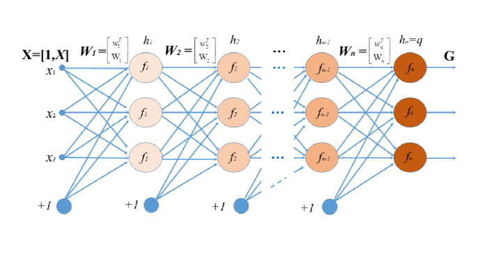
Figure 1: A fully-connected $n$-layer feedforward network.

3 Network Learning by Solving the System of Linear Equations

3.1 Single-Layer Network

Consider a single-layer FFN given by

$${\bf G}=f_{1}({\bf X}\boldsymbol{W}_{1}),$$ (16)

where $f_{1}(\cdot)$ is an activation function which operates elementwise on its matrix domain, ${\bf X}\in\mbox{$\mathbb{R}$}^{m\times(d+1)}$ is an augmented input (which includes the bias term), $\boldsymbol{W}_{1}\in\mbox{$\mathbb{R}$}^{(d+1)\times h_{1}}$ is the weight matrix to be estimated, and ${\bf G}\in\mbox{$\mathbb{R}$}^{m\times q}$ is the network output.

Let ${\bf Y}\in\mbox{$\mathbb{R}$}^{m\times q}$ be the target output to be learned. Mathematically, the learning problem is formulated as putting ${\bf G}={\bf Y}$ and then solve for the adjustable parameters within the model ${\bf G}$. Suppose $f_{1}$ satisfies the assumption given by:

Assumption 1

The function $f_{1}$ operates elementwise on matrices so that
$f_{1}({\bf X}\boldsymbol{W}_{1})={\bf Y}$ implies that there exists a full rank matrix ${\bf A}_{1}$ such that
${\bf A}_{1}\textbf{{W}}_{1}=\phi_{1}({\bf Y})$ where $\textbf{{W}}_{1}$ is an elementwise transformed version of $\boldsymbol{W}_{1}$ and $\phi_{1}$ is a monotonic and injective function that operates elementwise on its matrix domain.

This means that if the function $f_{1}$ is invertible, then $\phi_{1}(f_{1}({\bf X}\boldsymbol{W}_{1}))=\phi_{1}({\bf Y})$ implies that ${\bf X}\boldsymbol{W}_{1}=f^{-1}_{1}({\bf Y})$ where ${\bf A}_{1}={\bf X}$ and $\textbf{{W}}_{1}=\boldsymbol{W}_{1}$. If $f_{1}$ is not invertible, then there exists a transformation $\phi_{1}:\mbox{$\mathbb{R}$}\mapsto\mbox{$\mathbb{R}$}_{+}$ such that $\phi_{1}(f_{1}({\bf X}\boldsymbol{W}_{1}))={\bf A}_{1}\textbf{{W}}_{1}$ where ${\bf A}_{1}=\phi_{1}(f_{1}({\bf X}))$ and $\textbf{{W}}_{1}=\phi_{1}(f_{1}({\bf X}\boldsymbol{W}_{1}))/\phi_{1}(f_{1}({\bf X}))$ (assuming elementwise operation of the division). Since $\phi_{1}$ is a monotonic and injective function, the relative numerical order of elements within ${\bf X}$ and ${\bf Y}$ is unaltered. This means that the mapping between the data and the target can be fully recovered when $\phi_{1}$ is known (a good example is $\phi_{1}(\cdot)=\exp(\cdot)$). With this assumption on the property of $f_{1}$, the following result is obtained.

Theorem 1

Suppose $f_{1}$ satisfies Assumption 1. Then learning of the weights in the single-layer network of (16) admits the solution

$${\textbf{{W}}_{1}}={\bf A}_{1}^{{\dagger}}\phi_{1}({\bf Y})$$ (17)

in the sense of least squares error approximation to the target ${\bf Y}$ where ${\bf A}_{1}^{{\dagger}}=({\bf A}_{1}^{T}{\bf A}_{1})^{-1}{\bf A}_{1}^{T}$ when ${\bf A}_{1}^{T}{\bf A}_{1}$ has full rank, or ${\bf A}_{1}^{{\dagger}}={\bf A}_{1}^{T}({\bf A}_{1}{\bf A}_{1}^{T})^{-1}$ when ${\bf A}_{1}{\bf A}_{1}^{T}$ has full rank.

Proof: For an over-determined system learning a target output ${\bf Y}\in\mbox{$\mathbb{R}$}^{m\times q}$, we can put ${\bf G}={\bf Y}$ and learn the system by manipulating the kernel and the range space using

$$\phi_{1}({\bf Y})={\bf A}_{1}\textbf{{W}}_{1},$$ (18)

where the transformed weight matrix can be solved analytically as follows:

$${\bf A}_{1}^{T}\phi_{1}({\bf Y}) = {\bf A}_{1}^{T}{\bf A}_{1}{\textbf{{W}}}_{1}$$

$$\Rightarrow\hskip 14.22636pt({\bf A}_{1}^{T}{\bf A}_{1})^{-1}{\bf A}_{1}^{T}\phi_{1}({\bf Y}) = {\textbf{{W}}_{1}}.$$ (19)

This is the well-known solution to least squares error approximation.

For under-determined systems, the problem can be solved by putting

$${\textbf{{W}}}_{1}={\bf A}_{1}^{T}{\bf V}$$ (20)

where ${\bf V}\in\mbox{$\mathbb{R}$}^{m\times q}$ is obtained from

$$\phi_{1}({\bf Y}) = {\bf A}_{1}{\bf A}_{1}^{T}{\bf V}$$

$$\Rightarrow\hskip 14.22636pt({\bf A}_{1}{\bf A}_{1}^{T})^{-1}\phi_{1}({\bf Y}) = {\bf V}.$$ (21)

Putting (21) into (20) gives

$${\textbf{{W}}_{1}}={\bf A}_{1}^{T}({\bf A}_{1}{\bf A}_{1}^{T})^{-1}\phi_{1}({\bf Y}).$$ (22)

A direct substitution of (22) into the trace of $(\phi_{1}({\bf Y})-{\bf A}_{1}{\textbf{{W}}}_{1})^{T}(\phi_{1}({\bf Y})-{\bf A}_{1}{\textbf{{W}}}_{1})$ shows that the solution also minimizes the sum of squared errors. This completes the proof.  $\blacksquare$

Remark 1: Collectively, ${\bf A}_{1}^{{\dagger}}$, which is obtained by either (3.1) or (22), can be taken as the Moore-Penrose inverse of ${\bf A}_{1}$ [27]. The transformation of ${\bf Y}=f_{1}({\bf X}\boldsymbol{W}_{1})$ into (18) makes the system of nonlinear equations into a linear one. This shows that learning of an FFN of single connection layer (16) boils down to linear least squares estimation. Since both $\textbf{{W}}_{1}$ (transformed by $\phi_{1}$) and $\boldsymbol{W}_{1}$ (the non-transformed one) refer to the same set of weights of the network, we shall not distinguish between them and use only $\boldsymbol{W}_{k}$, $k=1,\cdots,n$ for subsequent development.  $\square$

3.2 Two-Layer Network

Next, consider a two-layer network given by

$${\bf G}=f_{2}([{\bf 1},f_{1}({\bf X}\boldsymbol{W}_{1})]\boldsymbol{W}_{2}),$$ (23)

where $f_{1}$ and $f_{2}$ are activation functions which operate elementwise upon their matrix domain, ${\bf X}\in\mbox{$\mathbb{R}$}^{m\times(d+1)}$ is an augmented input, $\boldsymbol{W}_{1}\in\mbox{$\mathbb{R}$}^{(d+1)\times h_{1}}$ and $\boldsymbol{W}_{2}\in\mbox{$\mathbb{R}$}^{(h_{1}+1)\times q}$ are the unknown network weights, ${\bf 1}=[1,...,1]^{T}\in\mbox{$\mathbb{R}$}^{m\times 1}$ is the bias vector, and ${\bf G}\in\mbox{$\mathbb{R}$}^{m\times q}$ denotes the network output. The target to be learned is ${\bf Y}\in\mbox{$\mathbb{R}$}^{m\times q}$.

The following assumption is needed for our learning formulation when the network output ${\bf G}=f_{2}([{\bf 1},f_{1}({\bf X}\boldsymbol{W}_{1})]\boldsymbol{W}_{2})$ is equated to the learning target ${\bf Y}$ in order to solve for the weight parameters.

Assumption 2

The functions $f_{1}$ and $f_{2}$ operate elementwise on matrices so that $f_{2}([{\bf 1},f_{1}({\bf X}\boldsymbol{W}_{1})]\boldsymbol{W}_{2})={\bf Y}$ implies that for known $\boldsymbol{W}_{1}$, there exists a full rank matrix ${\bf A}_{2}$ such that ${\bf A}_{2}\boldsymbol{W}_{2}=\phi_{2}({\bf Y})$ where ${\bf A}_{2}=[{\bf 1},f_{1}({\bf X}\boldsymbol{W}_{1})]$ and $\phi_{2}$ is a monotonic and injective function that operates elementwise on its matrix domain.

This means that $f_{2}$ can either be inverted (which results in $\phi_{2}(\cdot)=f^{-1}_{2}(\cdot)$) or transformed (in case of non-invertible) giving $[{\bf 1},f_{1}({\bf X}\boldsymbol{W}_{1})]\boldsymbol{W}_{2}=\phi_{2}({\bf Y})$ where $f_{1}$ provides sufficient rank conditioning regarding the matrix $[{\bf 1},f_{1}({\bf X}\boldsymbol{W}_{1})]$ for solving the linear equation using either the kernel or the range space. By separately considering the weights corresponding to the output bias term, we can partition $\boldsymbol{W}_{2}=\left[\begin{array}[]{c}{\bf w}_{2}^{T}\\ \textsf{W}_{2}\\ \end{array}\right]$ where ${\bf w}_{2}\in\mbox{$\mathbb{R}$}^{q\times 1}$ and $\textsf{W}_{2}\in\mbox{$\mathbb{R}$}^{h_{1}\times q}$. Based on these partitioned weights, we have

$$\phi_{2}({\bf Y}) = {\bf 1}\cdot{\bf w}_{2}^{T}+f_{1}({\bf X}\boldsymbol{W}_{1})\textsf{W}_{2}$$

$$\Rightarrow\hskip 14.22636pt\left[\phi_{2}({\bf Y})-{\bf 1}\cdot{\bf w}_{2}^{T}\right]\textsf{W}_{2}^{{\dagger}} = f_{1}({\bf X}\boldsymbol{W}_{1}),$$ (24)

where the symbol $\textsf{W}_{2}^{{\dagger}}$ denotes the Moore-Penrose inverse of the weights without bias, $\textsf{W}_{2}$.

Consider Assumption 1 and suppose $\boldsymbol{W}_{2}$ is known, then the hidden layer weights $\boldsymbol{W}_{1}$ can be solved by another inversion or transformation of equation (24) with respect to $f_{1}$:

$$\phi_{1}\left(\left[\phi_{2}({\bf Y})-{\bf 1}\cdot{\bf w}_{2}^{T}\right]\textsf{W}_{2}^{{\dagger}}\right) = {\bf X}\boldsymbol{W}_{1}$$

$$\Rightarrow\hskip 14.22636pt{\bf X}^{{\dagger}}\phi_{1}\left(\left[\phi_{2}({\bf Y})-{\bf 1}\cdot{\bf w}_{2}^{T}\right]\textsf{W}_{2}^{{\dagger}}\right) = {\boldsymbol{W}_{1}}.$$ (25)

After having $\boldsymbol{W}_{1}$ computed, it can be used to re-compute $\boldsymbol{W}_{2}$ as follows:

$$\phi_{2}({\bf Y}) = [{\bf 1},f_{1}({\bf X}{\boldsymbol{W}_{1}})]\boldsymbol{W}_{2}$$

$$\Rightarrow\hskip 14.22636pt\left[{\bf 1},f_{1}({\bf X}{\boldsymbol{W}_{1}})\right]^{{\dagger}}\phi_{2}({\bf Y}) = {\boldsymbol{W}_{2}}$$ (26)

where $[{\bf 1},f({\bf X}{\boldsymbol{W}_{1}})]^{{\dagger}}$ denotes the Moore-Penrose inverse of $[{\bf 1},f({\bf X}{\boldsymbol{W}_{1}})]$.

Theorem 2

Suppose $f_{1}$ and $f_{2}$ satisfy Assumptions 1–2. Then, learning of the fully-connected two-layer network (23) in terms of the least squares error approximation to target ${\bf Y}\in\mbox{$\mathbb{R}$}^{m\times q}$ boils down to solving the cross-coupling equations

$$\boldsymbol{W}_{1} = {\bf X}^{{\dagger}}\phi_{1}\left(\left[\phi_{2}({\bf Y})-{\bf 1}\cdot{\bf w}_{2}^{T}\right]\textsf{W}_{2}^{{\dagger}}\right),$$ (27)

$$\textrm{and}\ \ \boldsymbol{W}_{2}=\left[\begin{array}[]{c}{\bf w}_{2}^{T}\\ {\textsf{W}_{2}}\\ \end{array}\right] = \left[{\bf 1},f_{1}({\bf X}\boldsymbol{W}_{1})\right]^{{\dagger}}\phi_{2}({\bf Y}).$$ (30)

Proof: Equation (27) is obtained following the derivation steps in (24) through (25). Equation (30) has been derived in (26).  $\blacksquare$

Remark 2: This result shows that the two-layer network learning problem boils down to solving a system of equations with cross-coupling weights, i.e., $\boldsymbol{W}_{1}$ and $\boldsymbol{W}_{2}$ being inter-dependent. This implies that the system is recursive unless one of the two weight matrices is prefixed. We shall observe in Section 3.4 regarding the network representation capability when the hidden weights are prefixed randomly.  $\square$

3.3 Three-Layer Network and Beyond

Consider a three-layer network given by

$${\bf G}=f_{3}(\left[{\bf 1},f_{2}([{\bf 1},f_{1}({\bf X}\boldsymbol{W}_{1})]\boldsymbol{W}_{2})\right]\boldsymbol{W}_{3})$$ (31)

where ${\bf X}\in\mbox{$\mathbb{R}$}^{m\times(d+1)}$, $\boldsymbol{W}_{1}\in\mbox{$\mathbb{R}$}^{(d+1)\times h_{1}}$, $\boldsymbol{W}_{2}\in\mbox{$\mathbb{R}$}^{(h_{1}+1)\times h_{2}}$, $\boldsymbol{W}_{3}\in\mbox{$\mathbb{R}$}^{(h_{2}+1)\times q}$, ${\bf 1}=[1,...,1]^{T}\in\mbox{$\mathbb{R}$}^{m\times 1}$, and output ${\bf G}\in\mbox{$\mathbb{R}$}^{m\times q}$ with target ${\bf Y}\in\mbox{$\mathbb{R}$}^{m\times q}$. Following the assumption in the two-layer case, we have

Assumption 3

The functions $f_{i}$, $i=1,2,3$ operate elementwise on matrices so that $f_{3}(\left[{\bf 1},f_{2}([{\bf 1},f_{1}({\bf X}\boldsymbol{W}_{1})]\boldsymbol{W}_{2})\right]\boldsymbol{W}_{3})={\bf Y}$ implies that for known $\boldsymbol{W}_{j}$, $j=1,\cdots,k-1$, there is a full rank matrix ${\bf A}_{k}$ such that ${\bf A}_{k}\boldsymbol{W}_{k}={\bf B}_{k}$ for each $k=2,3$ where
${\bf A}_{2}=[{\bf 1},f_{1}({\bf X}\boldsymbol{W}_{1})]$, ${\bf A}_{3}=[{\bf 1},f_{2}([{\bf 1},f_{1}({\bf X}\boldsymbol{W}_{1})]){\boldsymbol{W}_{2}}]$,
${\bf B}_{2}=\phi_{2}(\phi_{3}({\bf Y})\boldsymbol{W}_{3}^{{\dagger}})$, ${\bf B}_{3}=\phi_{3}({\bf Y})$,
and $\phi_{k}$, $k=2,3$ are monotonic and injective functions that operate elementwise on their matrix domain.

This implies that $f_{1}$ in ${\bf A}_{2}$ and $f_{2}$ in ${\bf A}_{3}$ are functions that provide rank sufficiency for solving the system of linear equations. Then, similar to the two-layer network, the weights corresponding to the output bias term can be separated out as $\boldsymbol{W}_{3}=\left[\begin{array}[]{c}{\bf w}_{3}^{T}\\ \textsf{W}_{3}\\ \end{array}\right]$ where ${\bf w}_{3}\in\mbox{$\mathbb{R}$}^{q\times 1}$ and $\textsf{W}_{3}\in\mbox{$\mathbb{R}$}^{h_{2}\times q}$. By replacing ${\bf G}$ with ${\bf Y}$ and taking the transformation or inverse function of $f_{3}$ (i.e., $\phi_{3}$) to both sides of (31) after moving the bias weights over to the left hand side, we have

$$\phi_{3}({\bf Y})-{\bf 1}\cdot{\bf w}_{3}^{T} = f_{2}([{\bf 1},f_{1}({\bf X}\boldsymbol{W}_{1})]\cdot\boldsymbol{W}_{2})\textsf{W}_{3}$$

$$\Rightarrow\hskip 14.22636pt\left[\phi_{3}({\bf Y})-{\bf 1}\cdot{\bf w}_{3}^{T}\right]\textsf{W}_{3}^{{\dagger}} = f_{2}([{\bf 1},f_{1}({\bf X}\boldsymbol{W}_{1})]\cdot\boldsymbol{W}_{2})$$

$$\Rightarrow\hskip 14.22636pt\phi_{2}\left(\left[\phi_{3}({\bf Y})-{\bf 1}\cdot{\bf w}_{3}^{T}\right]\textsf{W}_{3}^{{\dagger}}\right) = [{\bf 1},f_{1}({\bf X}\boldsymbol{W}_{1})]\cdot\boldsymbol{W}_{2}.$$ (32)

Consider again the case of separating the bias weights in the middle layer:

$$\phi_{2}\left(\left[\phi_{3}({\bf Y})-{\bf 1}\cdot{\bf w}_{3}^{T}\right]\textsf{W}_{3}^{{\dagger}}\right)-{\bf 1}\cdot{\bf w}_{2}^{T} = f_{1}({\bf X}\boldsymbol{W}_{1})\textsf{W}_{2}$$

$$\Rightarrow\hskip 14.22636pt\left[\phi_{2}\left(\left[\phi_{3}({\bf Y})-{\bf 1}\cdot{\bf w}_{3}^{T}\right]\textsf{W}_{3}^{{\dagger}}\right)-{\bf 1}\cdot{\bf w}_{2}^{T}\right]\textsf{W}_{2}^{{\dagger}} = f_{1}({\bf X}\boldsymbol{W}_{1})$$

$$\phi_{1}\left\{\left[\phi_{2}\left(\left[\phi_{3}({\bf Y})-{\bf 1}\cdot{\bf w}_{3}^{T}\right]\textsf{W}_{3}^{{\dagger}}\right)-{\bf 1}\cdot{\bf w}_{2}^{T}\right]\textsf{W}_{2}^{{\dagger}}\right\} = {\bf X}\boldsymbol{W}_{1}$$

$$\Rightarrow\hskip 14.22636pt{\bf X}^{{\dagger}}\phi_{1}\left\{\left[\phi_{2}\left(\left[\phi_{3}({\bf Y})-{\bf 1}\cdot{\bf w}_{3}^{T}\right]\textsf{W}_{3}^{{\dagger}}\right)-{\bf 1}\cdot{\bf w}_{2}^{T}\right]\textsf{W}_{2}^{{\dagger}}\right\} = {\boldsymbol{W}_{1}}.$$ (33)

By initializing $\boldsymbol{W}_{2}$ and $\boldsymbol{W}_{3}$, the hidden weights $\boldsymbol{W}_{1}$ can be estimated using (33). After $\boldsymbol{W}_{1}$ has been estimated, $\boldsymbol{W}_{2}$ can be computed based on (32) as follows:

$$\phi_{2}\left(\left[\phi_{3}({\bf Y})-{\bf 1}\cdot{\bf w}_{3}^{T}\right]\textsf{W}_{3}^{{\dagger}}\right) = [{\bf 1},f_{1}({\bf X}{\boldsymbol{W}_{1}})]\cdot\boldsymbol{W}_{2}$$

$$\left[{\bf 1},f_{1}({\bf X}{\boldsymbol{W}_{1}})\right]^{{\dagger}}\phi_{2}\left(\left[\phi_{3}({\bf Y})-{\bf 1}\cdot{\bf w}_{3}^{T}\right]\textsf{W}_{3}^{{\dagger}}\right) = {\boldsymbol{W}_{2}}$$ (34)

Once the weight matrices $\boldsymbol{W}_{1}$ and $\boldsymbol{W}_{2}$ are estimated, the output weights can be determined as

$${\boldsymbol{W}_{3}}=\left[{\bf 1},f_{2}([{\bf 1},f_{1}({\bf X}{\boldsymbol{W}_{1}})]\cdot{\boldsymbol{W}_{2}})\right]^{{\dagger}}\phi_{3}({\bf Y}).$$ (35)

The solution given by (35) boils down to least squares error approximation because according to Lemma 1, multiplying the data matrix to both sides of (31) is equivalent to projecting the original equation onto the normal equation of sum of squared errors minimization [24]. With this observation on the three-layer network, we can generalize it to $n$-layer networks based on the following assumption.

Assumption 4

The functions $f_{i}$, $i=1,\cdots,n$ operate elementwise on matrices so that $f_{n}(\cdots\left[{\bf 1},f_{2}([{\bf 1},f_{1}({\bf X}\boldsymbol{W}_{1})]\boldsymbol{W}_{2})\right]\cdots\boldsymbol{W}_{n})={\bf Y}$ implies that for known $\boldsymbol{W}_{j}$, $j=1,\cdots,k-1$, there is a full rank matrix ${\bf A}_{k}$ such that ${\bf A}_{k}\boldsymbol{W}_{k}={\bf B}_{k}$ for each $k=2,\cdots,n$ where
${\bf A}_{2}=[{\bf 1},f_{1}({\bf X}\boldsymbol{W}_{1})]$, $\cdots$, ${\bf A}_{n}=[{\bf 1},f_{n-1}(\cdots[{\bf 1},f_{2}([{\bf 1},f_{1}({\bf X}\boldsymbol{W}_{1})]\boldsymbol{W}_{2})]\cdots\boldsymbol{W}_{n-1})]$,
${\scriptsize{\bf B}_{2}=\phi_{1}\left(\left[\phi_{2}(\cdots\left[\phi_{n-1}(\left[\phi_{n}({\bf Y})-{\bf 1}\cdot{\bf w}_{n}^{T}\right]\textsf{\small W}_{n}^{{\dagger}})-{\bf 1}\cdot{\bf w}_{n-1}^{T}\right]\textsf{\small W}_{n-1}^{{\dagger}}\cdots)-{\bf 1}\cdot{\bf w}_{2}^{T}\right]\textsf{\small W}_{2}^{{\dagger}}\right)}$,
$\cdots$, ${\bf B}_{n}=\phi_{n}({\bf Y})$,
and $\phi_{k}$, $k=2,\cdots,n$ are monotonic and injective functions that operate elementwise on their matrix domain.

Theorem 3

Suppose $f_{1}\cdots f_{n}$ satisfy Assumptions 1–4. Consider the fully-connected $n$-layer network given by

$${\bf G}=f_{n}\left([{\bf 1},f_{n-1}(\cdots\left[{\bf 1},f_{2}([{\bf 1},f_{1}({\bf X}\boldsymbol{W}_{1})]\cdot\boldsymbol{W}_{2})\right]\cdots\boldsymbol{W}_{n-1})]\cdot\boldsymbol{W}_{n}\right),$$ (36)

where ${\bf X}\in\mbox{$\mathbb{R}$}^{m\times(d+1)}$, $\boldsymbol{W}_{1}\in\mbox{$\mathbb{R}$}^{(d+1)\times h_{1}}$, $\boldsymbol{W}_{2}\in\mbox{$\mathbb{R}$}^{(h_{1}+1)\times h_{2}}$, $\cdots$, $\boldsymbol{W}_{n-1}\in\mbox{$\mathbb{R}$}^{(h_{n-2}+1)\times h_{n-1}}$, $\boldsymbol{W}_{n}\in\mbox{$\mathbb{R}$}^{(h_{n-1}+1)\times q}$, ${\bf 1}=[1,...,1]^{T}\in\mbox{$\mathbb{R}$}^{m\times 1}$, and output ${\bf G}\in\mbox{$\mathbb{R}$}^{m\times q}$ with target ${\bf Y}\in\mbox{$\mathbb{R}$}^{m\times q}$. Then, learning of the weights in (36) in terms of the least squares error approximation boils down to solving the following set of cross-coupling equations

$$\begin{array}[]{ccl}\boldsymbol{W}_{1}&=&{\bf X}^{{\dagger}}\phi_{1}\left(\left[\phi_{2}(\cdots\left[\phi_{n-1}(\left[\phi_{n}({\bf Y})-{\bf 1}\cdot{\bf w}_{n}^{T}\right]\textsf{W}_{n}^{{\dagger}})-{\bf 1}\cdot{\bf w}_{n-1}^{T}\right]\textsf{W}_{n-1}^{{\dagger}}\cdots)-{\bf 1}\cdot{\bf w}_{2}^{T}\right]\textsf{W}_{2}^{{\dagger}}\right),\\ \boldsymbol{W}_{2}&=&\left[{\bf 1},f_{1}({\bf X}\boldsymbol{W}_{1})\right]^{{\dagger}}\phi_{2}\left(\left[\phi_{3}(\cdots\left[\phi_{n-1}(\left[\phi_{n}({\bf Y})-{\bf 1}\cdot{\bf w}_{n}^{T}\right]\textsf{W}_{n}^{{\dagger}})-{\bf 1}\cdot{\bf w}_{n-1}^{T}\right]\textsf{W}_{n-1}^{{\dagger}}\cdots\right.\right.\\ &&\left.\left.\hskip 301.5992pt)-{\bf 1}\cdot{\bf w}_{3}^{T}\right]\textsf{W}_{3}^{{\dagger}}\right),\\ &\vdots&\\ \boldsymbol{W}_{n-1}&=&\left[{\bf 1},f_{n-2}([\cdots f_{2}([{\bf 1},f_{1}({\bf X}\boldsymbol{W}_{1})]\boldsymbol{W}_{2})]\cdots\boldsymbol{W}_{n-2})\right]^{{\dagger}}\phi_{n-1}\left(\left[\phi_{n}({\bf Y})-{\bf 1}\cdot{\bf w}_{n}^{T}\right]\textsf{W}_{n}^{{\dagger}}\right),\\ \boldsymbol{W}_{n}&=&\left[\begin{array}[]{c}{\bf w}_{n}^{T}\\ \textsf{W}_{n}\\ \end{array}\right]=\left[{\bf 1},f_{n-1}(\cdots[{\bf 1},f_{2}([{\bf 1},f_{1}({\bf X}\boldsymbol{W}_{1})]\boldsymbol{W}_{2})]\cdots\boldsymbol{W}_{n-1})\right]^{{\dagger}}\phi_{n}({\bf Y}).\end{array}$$ (37)

Proof: The proof follows from the derivation of the three-layer network by transforming or inverting all the activation functions of every layer to express $\boldsymbol{W}_{1}$ in terms of the sub-matrices $\textsf{W}_{2}$,…$\textsf{W}_{n}$ and vectors ${\bf w}_{2}$,…,${\bf w}_{n}$. Then $\boldsymbol{W}_{2}$ is constructed based on $\boldsymbol{W}_{1}$, $\textsf{W}_{3}$,…$\textsf{W}_{n}$ and ${\bf w}_{3}$,…,${\bf w}_{n}$ with activation one layer near the inputs untransformed or un-inverted. The estimation of each increment of the weight layer comes with one layer near the inputs untransformed or un-inverted. Such construction follows through till $\boldsymbol{W}_{n}$. Hence the result.  $\blacksquare$

With this result, we propose a single pass algorithm for multilayer network learning based on the Kernel-And-Range (KAR) space as follows.

Algorithm	:	KARnet
Initialization	:	Assign random weights to $\textsf{W}_{2},\cdots,\textsf{W}_{n}$ and ${\bf w}_{2}$,…,${\bf w}_{n}$.
Learning	:	Compute the network weights $\boldsymbol{W}_{1}$,…$\boldsymbol{W}_{n}$ sequentially using (37)
		with $f=f_{1}=\cdots=f_{n}$ using ‘logit’ activation and
		$\phi=\phi_{1}=\cdots=\phi_{n}$ using ‘sigmoid’ transformation.
Net output	:	Compute the network output ${\bf G}$ according to (36).

Remark 3: Theorem 3 shows that the FFN network learning problem is a cross-coupling one, with weights in each layer depending on each and every other layers. For the proposed learning, the learning outcome is dependent on the initialization of the weight terms $\textsf{W}_{2},\cdots,\textsf{W}_{n}$ and ${\bf w}_{2}$,…,${\bf w}_{n}$. For simplicity in terms of implementation, we shall investigate into a random initialization of these weight terms even though the algorithm does not impose such a limitation. The representation of such a randomized network shall be investigated in the sequel.  $\square$

3.4 Network Representation

Here, we show the network representation capability before the experiments. In our notations, the function $f=f_{1}=\cdots=f_{n}$ is operated elementwise on the matrix domain.

Theorem 4

(Two-layer Network) Given $m$ distinct data samples of multivariate inputs with univariate output and suppose $f_{1}({\bf X}\boldsymbol{W}_{1})$ has full rank. Then there exists a fully-connected two-layer network of linear output with at least $m$ adjustable weights that can represent these data samples.

Proof: Consider an augmented set of inputs, then the 2-layer network of linear output can be written as:

$$\boldsymbol{g}=f_{1}({\bf X}\boldsymbol{W}_{1})\boldsymbol{w}_{2},$$ (38)

where ${\bf X}\in\mbox{$\mathbb{R}$}^{m\times(d+1)}$ is the augmented network input matrix, $\boldsymbol{W}_{1}\in\mbox{$\mathbb{R}$}^{(d+1)\times h_{1}}$ contains the hidden weights, $\boldsymbol{w}_{2}\in\mbox{$\mathbb{R}$}^{h_{1}\times 1}$ contains the output weights, and $\boldsymbol{g}\in\mbox{$\mathbb{R}$}^{m\times 1}$ is the network output vector. Since $f_{1}({\bf X}\boldsymbol{W}_{1})$ is assumed to be of full rank for the given data and weight matrix, it turns out that only $m$ elements are required for $\boldsymbol{w}_{2}$ (i.e., $h_{1}=m$) for solving ${\bf y}=f_{1}({\bf X}\boldsymbol{W}_{1})\boldsymbol{w}_{2}$ uniquely given any target vector ${\bf y}$. Hence the proof.  $\blacksquare$

Theorem 5

(Multilayer Network) Given $m$ distinct samples of input-output data pairs and suppose the adopted activation function satisfies Assumption 4. Then there exists a fully-connected $n$-layer network of $q$ outputs with at least $m\times q$ adjustable weights that can represent these data samples.

Proof: By adopting a recursive notation of ${\bf A}_{k}=f_{k}([{\bf 1},{\bf A}_{k-1}]\boldsymbol{W}_{k})$ for $k=2,3,\cdots,n-2,n-1$ with ${\bf A}_{1}=f_{1}({\bf X}\boldsymbol{W}_{1})$, the $n$-layer network can be written as

$$\boldsymbol{G}=f_{n}([{\bf 1},{\bf A}_{n-1}]\boldsymbol{W}_{n})\ \ \ \in\mbox{$\mathbb{R}$}^{m\times q}.$$ (39)

Consequently, (39) can be viewed as a system of linear equations to learn the weight matrix $\boldsymbol{W}_{n}\in\mbox{$\mathbb{R}$}^{h_{n-1}\times q}$ for fitting the target ${\bf Y}\in\mbox{$\mathbb{R}$}^{m\times q}$ based on the transformation using $\phi_{n}$:

$$\phi_{n}({\bf Y})=[{\bf 1},{\bf A}_{n-1}]\boldsymbol{W}_{n}.$$ (40)

To fully represent the $m$ number of data points labelled by $\phi_{n}({\bf Y})$, the matrix $[{\bf 1},{\bf A}_{n-1}]$ needs to have at least rank $m$. This means that the output weight matrix $\boldsymbol{W}_{n}$ requires at least $m$ (i.e., $h_{n-1}+1=m$) adjustable weight elements for each of its $q$ columns corresponding to the output dimension. As for the inner layer weights $\boldsymbol{W}_{k}$, $k=1,\cdots,n-1$, an identity matrix of $m\times m$ size would be suffice for transferring the input information from the innermost layer to the $(n-1)^{th}$ layer. Since the compositional function $f_{n-1}(\cdots f_{1}({\bf X}\boldsymbol{W}_{1})\cdots)$ is of full rank according to Assumption 4, $[{\bf 1},{\bf A}_{n-1}]$ in (40) has full rank of size $m$. This means that $\boldsymbol{W}_{n}$ in (40) can be estimated uniquely.

In a nutshell, the $n$-layer network with $q$ outputs can be reduced to $q$ number of the single-output network of two-layer in (38) where each output requires $m$ number of adjustable weights. Hence the proof.  $\blacksquare$

3.5 Towards Understanding of Network Generalization

In view of the good results observed in deep learning despite the huge number of weight parameters, many attempts can be found in studying the generalization property of deep networks (see e.g., [36, 37, 38, 39, 40, 41, 42, 43, 44, 45, 46]). Based on our result on network representation, several properties related to network generalization are observed.

1. The array structure of the fully-connected network in matrix form plays a key role in constraining the complexity of model for approximation. Particularly, the number of hidden nodes in each layer ($h_{i}$, $i=1,2,...,n$) determines the column size of the weight matrix $\boldsymbol{W}_{i}$. This column size directly influences the effective parameter size in each layer. Hence, the effective number of parameters (and the complexity of approximation) does not grow exponentially (with the size of the gross network parameters) with respect to the number of layers.

2. Thanks to the high redundancy of weights within each column, such an array structure of the weight matrix offers numerous alternative solutions that attain the desired fitting result. This accounts for the ease of fitting even with random initialization of the weights (see the proposed algorithm and (37)) and leaves the remaining issue of generalization to the representativeness of the training data. This property shall be exploited in the algorithm for experimentation.

3. The representation capability of network is shown to be grounded upon the well-known theory of linear algebra. However to our surprise, the nonlinearity in the activation functions actually contributes to the well-posedness (such as making the matrix invertible) of the problem than otherwise.

4. Capitalized on the minimum norm property according to Lemma 1 and Lemma 2, no explicit regularization has been incorporated into the learning. The least squares approximation (section 2.1) in the primal space (with covariance matrix ${\bf A}^{T}{\bf A}\in\mbox{$\mathbb{R}$}^{d\times d}$ in (3)) and the dual space (with Gram matrix ${\bf A}{\bf A}^{T}\in\mbox{$\mathbb{R}$}^{m\times m}$ in (9)) has, indeed, long been known in the theory of linear systems [27]. Unfortunately, the effectiveness of such utilization of the primal-dual pair has been masked by the popularity of weight decay regularization. The observation in [35] which compares between the regularized results with those of non-regularized ones is not surprising due to the minimum norm solution nature (section 2.1) which has long been known in the statistical community.

Given the mapping capability of the network together with the above observations, we conjecture that network generalization is hinged upon the model complexity and the similarity/difference between the distributions of the training and testing data sets (such as optimism defined by [47]).

4 Case Study

In this study, we show case the results of the proposed learning algorithm KARnet on two benchmark examples. The goal of the first example is to observe the decision surface and the training CPU time for the compared methods on mapping linearly non-separable data. The chosen data set is the well-known XOR problem. The second example aims to validate the network representation theory. The chosen problem is the iris flower data set from the UCI machine learning repository [48]. All the experimental studies were carried out on an Intel Core i7-6500U CPU at 2.59GHz with 8G of RAM.

4.1 The XOR problem

In this example, the proposed learning algorithm KARnet and the conventional feedforwardnet from the Matlab toolbox [49] are evaluated in terms of their decision landscapes. Both the compared methods use the ‘logit’ (i.e., $f=\log(x/(1-x))$ as the activation function where its functional inverse is $f^{-1}=1/(1+e^{-x})=$ ‘sigmoid’) for $x\in[0,1)$. The training of feedforwardnet uses the default Levenberg-Marquardt ‘trainlm’ search and stopping. For both learning algorithms, a two-layer network with one hidden layer that consists of two nodes ($h_{1}=2$) and a five-layer network with each layer composing of five hidden nodes ($h_{1}=h_{2}=h_{3}=h_{4}=3$, $q=1$, we call it a 3-3-3-3-1 structure) are evaluated.

The learned decision surfaces for the two-layer KARnet and feedforwardnet are shown in Fig. 2(a) and (b) respectively. Due to the perfect symmetry of the XOR data points which can cause degenerative pseudoinverse computation, a small perturbation has been included to the data points where the training data points are $(x_{1},x_{2})\in$ $\{(0,0)$, $(0.9991,0.9991)$, $(0.9990,0)$, $(0,0.9990)\}$ for respective target values $y\in\{0,0,1,1\}$. The decision surface in Fig. 2(a) shows a perfect fitting of all the data points in the two classes for KARnet. Contrastingly, the decision surface of feedforwardnet in Fig. 2(b) shows a complex fitting of the data points. This could be due to an early stopping of search at steep error surface of the logit function. The trained outputs of the two-layer networks for the four data points are [$0$, $0$, 1, 1] and [$-0.0758$, $0.0665$, $0.4302$, $1.0988$] respectively for KARnet and feedforwardnet.

The learned output surfaces for the two five-layer networks namely, KARnet and feedforwardnet are shown in Fig. 2(c) and (d) respectively. The trained outputs for the five-layer KARnet and feedforwardnet are respectively [$0$, 0, 1, 1] and [$-0.1527$, 0.0331, $-0.2331$, 0.0296]. This result, again, shows inadequate stopping of the gradient-based search.

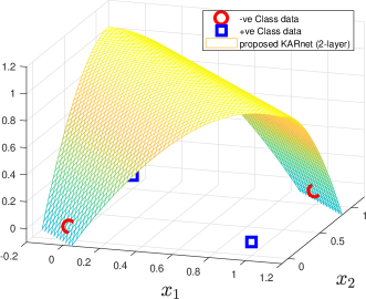
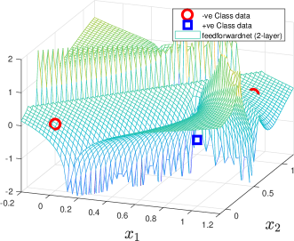
(a)	(b)
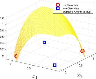
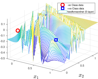
(c)	(d)

Figure 2: Decision surface plots of two-layer/five-layer feedforward networks (proposed KARnet($f=logit$, $f^{-1}=sigmoid$) and feedforwardnet) trained by the proposed method and trainlm.

For the two-layer networks, the clocked training CPU times are 0.0625 and 1.0781 seconds for KARnet and feedforwardnet respectively. For the five-layer networks, the training CPU times for KARnet and feedforwardnet are 0.1250 and 1.0938 seconds respectively. Certainly, these computational time results show the efficiency of the proposed training comparing with the gradient descent search even without optimizing our code implementation.

4.2 Network Representation: Iris Plant Data

The iris plant data is a well-known benchmark data set in classification with small sample size ($150$ in total) and small dimension ($d=4$). Among the 150 samples, each of the three categories ($q=3$) contains 50 samples. For illustration purpose, 90 samples (within which 30 samples per category) are used for training and the remaining 60 are used as test samples. A two-layer network is used in this study. In order to illustrate the systems of over-determined and under-determined cases, the number of nodes in the hidden layer is chosen as $h_{1}\in\{79,80,\cdots,93\}$. This gives a hidden weight $\boldsymbol{W}_{1}$ of size $(4+1)\times h_{1}$. Since the training sample size is $m=90$, the case for which $h_{1}=90$ is an equal-determined case in view of the output weights, whereas those with lower and higher sizes are respectively the over-determined and under-determined cases.

The two-layer network is learned using a randomized $\boldsymbol{W}_{1}$ with an one-versus-all indicator target. Fig. 3 shows two cases of learning outputs for $h_{1}=89$ (Fig. 3(a)) and $h_{1}=90$ (Fig. 3(b)). Here, we observe that the outputs have a perfect fit to all data samples when $h_{1}=90$. Conversely, we do not see a perfect fit when $h_{1}=89$ because there are more data than the number of effective parameters.

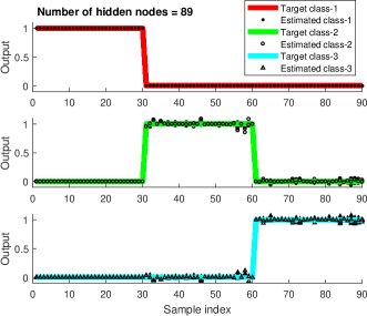
(a)	(b)

Figure 3: Target outputs and learned outputs of a 2-layer KARnet.

Fig. 4 shows 10 Monte Carlo trials of the quantitative fitting results in terms of the Sum of Squared Errors (SSE) and the classification error count rates for both training and testing. Based on the theory of representation, the two-layer network shall fit the target value of all the data samples when $h_{1}\geqslant m$ ($m=90$ here) for each of the 3 output columns. This is clearly observed from the SSE plot where SSE=0 is observed for $h_{1}\geqslant 90$. Since this is a classification problem, the training and test classification error rates are also included in the plot. These results show that the training has attained a zero classification error count while the test classification error rate is not significantly affected by the goodness of fit in terms of SSE.

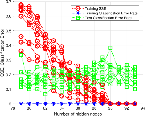
Figure 4: The SSE and the classification error count rates for a two-layer network

Next, we train a five-layer network with the first four layers having randomized weights. Except for $\boldsymbol{W}_{5}$, each of the weights $\boldsymbol{W}_{1}$, …, $\boldsymbol{W}_{4}$ has a similar column size to that of the first layer. Fig. 5 shows the SSE and classification error rates. This result shows that zero SSE can be attained at column size ($h_{i}$, $i=1,...,4$) lower than 90! This suggests the number of hidden weight nodes (columns) may be traded by the layer depth. This opens up an important topic for future study.

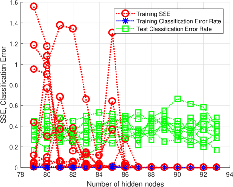
Figure 5: The SSE and the classification error count rates for a five-layer network

5 Experiments

In this section, the proposed learning algorithm KARnet is evaluated on real-world data sets taken from the public domain. Due to the limited computing facility (lack of GPU), only data sets ranging from small to medium sample sizes are considered. The goals of this experimentation include (i) to verify the practical feasibility of the formulation on real-world data of relatively small dimension ($d\leqslant 64$); (ii) if practically feasible, to observe how well it compares with the state-of-the-art backpropagation algorithm that utilizes the same ‘logit’ activation function with that in KARnet. (iii) to record the computational training CPU times for the proposed algorithm and the gradient based network learning counterpart. Since the fine tuning of network and learning generalization are topics for further research, the scope of current empirical investigation is limited to observing the practical feasibility, the basic behavior in terms of raw attainable accuracy without fine tuning, and the computational efficiency of the proposed algorithm. A total of 42 data sets from the UCI machine learning repository [48] are adopted for this study.

5.1 UCI Data Sets

The adopted data sets from the UCI machine learning repository [48] is summarized in Table 1 with their pattern attributes [50]. The experimental goals (i) and (ii) are evaluated by observing the prediction accuracy of the algorithm.

Table 1: Summary of UCI [48] data sets and chosen hidden layer sizes based on cross-validation within the training set

		(i)	(ii)	(iii)	(iv)	2-layer		3-layer	4-layer
						(hidd.size)	(hidd.size)	(hidd.size)	(hidd.size)
	Database name	#cases	#feat	#class	#miss	FFnet	KARnet	KARnet	KARnet
1.	Shuttle-l-control	279(15)	6	2	no	30	1	2	10
2.	BUPA-liver-disorder	345	6	2	no	80	2	1	2
3.	Monks-1	124(432)	6	2	no	20	3	1	1
4.	Monks-2	169(432)	6	2	no	30	1	500	500
5.	Monks-3	122(432)	6	2	no	30	80	1	3
6.	Pima-diabetes	768	8	2	no	80	2	1	10
7.	Tic-tac-toe	958	9	2	no	200	20	20	20
8.	Breast-cancer-Wiscn	683(699)	9(10)	2	16	50	1	1	20
9.	StatLog-heart	270	13	2	no	80	1	10	5
10.	Credit-app	653(690)	15	2	37	80	3	1	10
11.	Votes	435	16	2	yes	10	1	20	1
12.	Mushroom	5644(8124)	22	2	attr#11	200	1	30	5
13.	Wdbc	569	30	2	no	30	1	1	3
14.	Wpbc	194(198)	33	2	4	80	2	20	500
15.	Ionosphere	351	34	2	no	80	5	5	10
16.	Sonar	208	60	2	no	80	1	50	2
17.	Iris	150	4	3	no	500	5	5	2
18.	Balance-scale	625	4	3	no	500	20	100	3
19.	Teaching-assistant	151	5	3	no	500	2	80	200
20.	New-thyroid	215	5	3	no	500	30	5	2
21.	Abalone	4177	8	3(29)	no	80	10	20	3
22.	Contraceptive-methd	1473	9	3	no	5	80	10	5
23.	Boston-housing	506	12(13)	3(cont)	no	500	10	10	20
24.	Wine	178	13	3	no	500	5	5	5
25.	Attitude-smoking+	2855	13	3	no	2	1	50	10
26.	Waveform+	3600	21	3	no	50	80	10	5
27.	Thyroid+	7200	21	3	no	100	10	10	20
28.	StatLog-DNA+	3186	60	3	no	200	80	5	50
29.	Car	2782	6	4	no	500	50	500	500
30.	StatLog-vehicle	846	18	4	no	500	100	50	5
31.	Soybean-small	47	35	4	no	50	1	1	1
32.	Nursery	12960	8	4(5)	no	500	30	30	10
33.	StatLog-satimage+	6435	36	6	no	80	100	50	20
34.	Glass	214	9(10)	6	no	100	30	5	10
35.	Zoo	101	17(18)	7	no	100	500	10	80
36.	StatLog-image-seg	2310	19	7	no	100	100	50	20
37.	Ecoli	336	7	8	no	500	30	10	5
38.	LED-display+	6000	7	10	no	500	30	20	10
39.	Yeast	1484	8(9)	10	no	500	500	30	30
40.	Pendigit	10992	16	10	no	–	500	80	200
41.	Optdigit	5620	64	10	no	–	500	100	30
42.	Letter	20000	16	26	no	–	500	200	200

(i-iv)	:	(i) Total number of instances, i.e. examples, data points, observations (given number of instances). Note: the number of instances used is larger than the given number of instances when we expand those “don’t care” kind of attributes in some data sets; (ii) Number of features used, i.e. dimensions, attributes (total number of features given); (iii) Number of classes (assuming a discrete class variable); (iv) Missing features;
$+$	:	Accuracy measured from the given training and test set instead of 10-fold validation (for large data cases with test set containing at least 1,000 samples);
FFnet	:	The feedforwardnet from the Matlab’s toolbox;
hidd.size	:	For 3layer and 10layer networks, the number of hidden layer nodes are chosen similarly for simplicity of study;
Note	:	Data from the Attitudes Towards Smoking Legislation Survey - Metropolitan Toronto 1988, which was funded by NHRDP (Health and Welfare Canada), were collected by the Institute for Social Research at York University for Dr. Linda Pederson and Dr. Shelley Bull.

(i) The prediction performance

In this experiment, the prediction performance of the proposed KARnet is compared with that of the feedforwardnet from the Matlab’s toolbox [49] using a two-layer fully-connected network structure. Both the networks adopted the logit activation function in this study. The performance is evaluated based on 10 trials of 10-fold stratified cross-validation tests for each of the data set. The selection of the number of hidden nodes is based on another 10-fold cross-validation within the training set.

The chosen hidden node size (based on a search within the set $\{$1, 2, 3, 5, 10, 20, 30, 50, 80, 100, 200, 500$\}$ by cross-validation using only the training set) is shown in the third column-group of Table 1. For both the two-layer networks, the selected size of hidden nodes appear to be much different for KARnet and Feedforwardnet among the data sets. Apparently, there seems to have no correlation between the choice of hidden node sizes for the two networks. The choice of the size of the hidden nodes is dependent on the training accuracy where some data sets appear to be more over-fit than others.

The average results of prediction accuracies (based on 10 trials of 10-fold cross-validation) for such choice of hidden node size for KARnet and Feedforwardnet are shown in Fig. 6. For the Feedforwardnet, the accuracies of data sets 40, 41 and 42 are not available due to the “out of memory” limitation for the chosen network size of 500 hidden nodes on the current computing platform. From these results, the accuracies of KARnet appear to be significantly better than that of Feedforwardnet for most of the data sets. The gross average accuracies for KARnet and Feedforwardnet are respectively 79.39% and 66.99% based on the first 39 data sets. These results suggest relatively good generalization performance of KARnet than that of Feedforwardnet based on the chosen activation function.

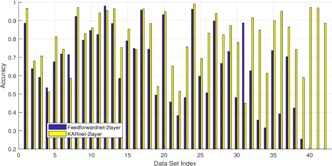
Figure 6: Comparing KARnet with Feedforwardnet at their best chosen hidden nodes size based on cross-validation using only the training data. The accuracies of data sets 40, 41 and 42 for Feedforwardnet are not shown due to the “out of memory” limitation for the current computing platform.

In the next experiment, we observe the generalization performance of KARnet when it uses the same hidden node size as that of Feedforwardnet. Fig. 7 shows the average accuracies of KARnet which are plotted along with those of Feedforwardnet. It is clear from the figure that KARnet outperforms Feedforwardnet for most data sets. The gross average accuracy for KARnet based on 39 data sets is 80.03% (comparing with 66.99% for Feedforwardnet).

Figure 7: Comparing the accuracy of KARnet with that of Feedforwardnet at the same hidden nodes size.

(ii) The training CPU time

After observing the feasibility of network learning on the UCI data sets, we move on to observe the training CPU time clocked for both the studied methods. Fig. 8 shows the training CPU times for KARnet and Feedforwardnet at their optimized hidden node size based on cross-validation using the training set. Fig. 9 shows the training CPU times at the same hidden node size for the two studied methods. For the optimized network size, the gross average CPU times over the first 39 data sets are respectively 0.0211 seconds and 180.37 seconds for KARnet and Feedforwardnet. When the KARnet uses the same network size with that of Feedforwardnet, the gross average CPU times over the first 39 data sets is 0.8003 seconds. This shows a 225 times faster in training speed for KARnet over Feedforwardnet. The gain from the training speed is attributed to the closed-form and non-iterative learning.

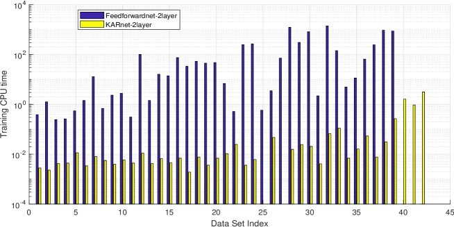
Figure 8: Comparing the training CPU time (seconds) of KARnet with that of Feedforwardnet at their cross-validation optimized size of hidden nodes.

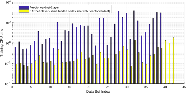
Figure 9: Comparing the training CPU time (seconds) of KARnet with that of Feedforwardnet when both the networks have the same size of hidden nodes.

(iii) The effect of deep layers

Having verified the feasibility and the prediction performance with the training processing time, we move a step further to observe the effect of a deeper structure utilizing an exponentially increasing number of hidden nodes towards the input layer. Specifically, the two-layer network uses a structure of $[h,\ q]$ for the hidden layer and the output layer respectively. The three-layer network uses a $[2\times h,\ h,\ q]$ structure and the four-layer network uses a $[4\times h,\ 2\times h,\ h,\ q]$ structure. The dimension of output is $q$, and $h$ is determined based on a cross-validation search within the training set for $h\in\{$1, 2, 3, 5, 10, 20, 30, 50, 80, 100, 200, 500$\}$. The prediction accuracies for KARnet with two-, three- and four-layers are shown in Fig. 10. Except for a few data sets, the results show insignificant variation of prediction accuracy according to the change in network depth.

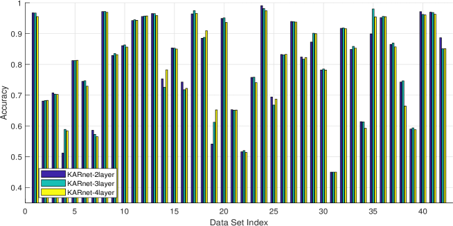
Figure 10: The effect of layers on accuracy performance.

5.2 Summary of Results and Discussion

With the experimental feasibility and learning efficiency validated, we shall summarize the results obtained, from both theoretical and experimental perspectives. The theoretical contributions of this work can be summarized as follows:

• Kernel-And-Range space estimation: A theoretical framework has been established to relate the solution given by the kernel-and-range space estimation to that based on the least squares error estimation. The importance of such an establishment is that it enables a gradient-free network learning process where the formally inevitable iterative search process can be by-passed.

• Understanding of FFN learning: The proposed kernel-and-range space estimation has been applied to multilayer network learning wherein an analytical formulation is obtained. Based on this formulation, we found that solving the network training problem boils down to solving a set cross-coupling system of linear equations for the feedforward structure.

• An analytic learning algorithm: Utilizing the above results, a single-pass algorithm has been proposed to train the multilayer feedforward network. Essentially, the algorithm capitalizes on the random initialization to decouple the process of network weight estimation. This has been grounded on the vast feasible solutions revealed by the analysis of network representation. Despite of its random initialization nature, the proposed network learning shows relatively good prediction performance compared with the conventional gradient based learning.

• Network representation: The capability of network representation has been shown to be dependent on the number of data samples and the number of output vectors. It has been discovered that the warping effect of the nonlinear activation function contributes to the well-posedness of the problem.

• Network generalization: Capitalized on the minimum norm property according to Lemma 1 and Lemma 2, no explicit regularization has been incorporated into the learning. The extensive experimental results provide relevant support towards this proposition.

To summarize the numerical evaluations, the following observations are made:

• Practical feasibility: The numerical feasibility of estimating the weights of the multilayer network without gradient descent has been verified by utilizing a randomly initialized estimation. Essentially, the estimation process has been expressed in closed-from with neither gradient derivation nor iterative search.

• Prediction accuracy: Utilizing the logit activation function, the results of numerical prediction based on the stratified cross-validation show good generalization performance for the proposed kernel-and-range estimation comparing with that of the error gradient based learning. It is not surprising to observe that such learning performance does not depend on explicit regularization.

• Training CPU time: Due to the analytical and non-iterative estimation, the training speed for the proposed method is over 200 times faster than the competing gradient-based learning when the same number of hidden nodes has been chosen for the compared algorithms.

• Impact of deeper structure: According to the results based on deeper networks with an exponentially increasing node size towards the input, the prediction performance does not seem to vary significantly for deeper networks.

6 Conclusion

We have established that the solution obtained from the kernel and range space manipulation is equivalent to that obtained by the least squares error estimation. This paved the ground for a gradient free parametric estimation when the system can be expressed in linear matrix form. The fully-connected feedforward neural network is a representative example for such a system. Based on the proposed kernel and range space manipulation, solving the weights of the fully-connected feedforward network is found to boil down to solving a cross-coupling equation. By initializing the weights in the hidden layers, the system can be decoupled with hidden weights obtained in an analytical form. In view of network representation, it has been found that the minimum number of parameters is determined by the number of layers and the number of outputs, thanks to the favorable warping effect of the nonlinear monotonic activations. The numerical evaluation on real-world benchmark data sets validated the feasibility of the formulation. This opens up the vast possibilities to expand the research direction.

References

- [1] H. J. Kelley, “Gradient theory of optimal flight paths,” Ars Journal, vol. 30, no. 10, pp. 947–954, 1960.
- [2] P. J. Werbos, “Beyond regression: New tools for prediction and analysis in the behavioral sciences,” Ph.D. dissertation, Beyond Regression: New Tools for Prediction and Analysis in the Behavioral Sciences, 1974.
- [3] R. Hecht-Nielsen, “Theory of the backpropagation neural network,” in Proceedings of International Joint Conference on Neural Networks (IJCNN), 1989, pp. 593–605.
- [4] P. J. Werbos, “Backpropagation: Past and future,” in Proceedings of the IEEE 1988 International Conference on Neural Networks (ICNN), 1988, pp. I–343–353.
- [5] ——, “Backpropagation through time: what it does and how to do it,” Neural Networks, vol. 78, no. 10, pp. 1550–1560, 1990.
- [6] S. O. Haykin, Neural Networks and Learning Machines. New York: Prentice Hall, 2009.
- [7] K.-I. Funahashi, “On the approximate realization of continuous mappings by neural networks,” Neural Networks, vol. 2, no. 3, pp. 183 –192, 1989.
- [8] K. Hornik, M. Stinchcombe, and H. White, “Multi-layer feedforward networks are universal approximators,” Neural Networks, vol. 2, no. 5, pp. 359–366, 1989.
- [9] G. Cybenko, “Approximations by superpositions of a sigmoidal function,” Math. Cont. Signal & Systems, vol. 2, pp. 303–314, 1989.
- [10] R. Hecht-Nielsen, “Kolmogorov’s mapping neural network existence theorem,” in Proceedings of IEEE First International Conference on Neural Networks (ICNN), vol. III, 1987, pp. 11–14.
- [11] R. Battiti, “First and second order methods for learning: Between steepest descent and newton s method,” Neural Computation, vol. 4, no. 2, pp. 141–166, 1992.
- [12] P. Patrick van der Smagt, “Minimisation methods for training feedforward neural networks,” Neural Networks, vol. 7, no. 1, pp. 1–11, 1994.
- [13] E. Barnard, “Optimization for training neural nets,” IEEE Trans. on Neural Networks, vol. 3, no. 2, pp. 232–240, 1992.
- [14] W. F. Schmidt, M. A. Kraaijveld, and R. P. W. Duin, “Feed forward neural networks with random weights,” in Proceedings of 11th IAPR Int. Conf. on Pattern Recognition., Conf. B: Pattern Recognition Methodology and Systems, Vol. 2, The Hague, 1992, pp. 1–4.
- [15] N. J. Guliyev and V. E. Ismailov, “A single hidden layer feedforward network with only one neuron in the hidden layer can approximate any univariate function,” Neural Computation, vol. 28, no. 7, pp. 1289–1304, 2016.
- [16] Y. Shang and B. W. Wah, “Global optimization for neural network training,” IEEE Computer, vol. 29, no. 3, pp. 45–54, Mar 1996.
- [17] Z. Tang and G. J. Koehler, “Deterministic global optimal fnn training algorithms,” Neural Networks, vol. 7, no. 2, pp. 301–311, 1994.
- [18] I. Goodfellow, Y. Bengio, and A. Courville, Deep Learning. MIT Press, 2016, http://www.deeplearningbook.org.
- [19] G. Taylor, R. Burmeister, Z. Xu, B. Singh, A. Patel, and T. Goldstein, “Training neural networks without gradients: A scalable ADMM approach,” in Proceedings of the 33rd International Conference on Machine Learning (ICML), vol. 48, New York, USA, 2016, pp. 2722–2731.
- [20] B. M. Wilamowski and H. Yu, “Neural network learning without backpropagation,” IEEE Trans. on Neural Networks, vol. 21, no. 11, pp. 1793–1803, 2010.
- [21] M. Jaderberg, W. M. Czarnecki, S. Osindero, O. Vinyals, A. Graves, D. Silver, and K. Kavukcuoglu, “Decoupled neural interfaces using synthetic gradients,” in Proceedings of the 34th International Conference on Machine Learning (PMLR), Sydney, Australia, 2017, pp. 1627–1635.
- [22] L. M. Rios and N. V. Sahinidis, “Derivative-free optimization: a review of algorithms and comparison of software implementations,” Journal of Global Optimization, vol. 56, pp. 1247–1293, 2013.
- [23] K.-A. Toh, “Learning from the kernel and the range space,” in Proceedings of the 17th IEEE/ACIS International Conference on Computer and Information Science, Singapore, June 2018, pp. 417–422.
- [24] G. Strang, Introduction to Linear Algebra, 5th ed. Wellesley: Wellesley-Cambridge Press, 2016.
- [25] W. R. Madych, “Solutions of underdetermined systems of linear equations,” in Lecture Notes – Monograph Series, Spatial Statistics and Imaging, 1991, vol. 20, pp. 227–238, institute of Mathematical Statistics.
- [26] S. Boyd and L. Vandenberghe, Convex Optimization. Cambridge: Cambridge University Press, 2004.
- [27] A. Albert, Regression and the Moore-Penrose Pseudoinverse. New York: Academic Press, Inc., 1972, vol. 94.
- [28] Adi Ben-Israel and Thomas N.E. Greville, Generalized Inverses: Theory and Applications, 2nd ed. New York: Springer-Verlag, 2003.
- [29] S. L. Campbell and C. D. Meyer, Generalized Inverses of Linear Transformations, (SIAM edition of the work published by Dover Publications, Inc., 1991) ed. Philadelphia, USA: Society for Industrial and Applied Mathematics, 2009.
- [30] R. O. Duda, P. E. Hart, and D. G. Stork, Pattern Classification, 2nd ed. New York: John Wiley & Sons, Inc, 2001.
- [31] K. B. Petersen and M. S. Pedersen, The Matrix Cookbook, 2006, http://www.mit.edu/ wingated/stuff_i_use/matrix_cookbook.pdf.
- [32] E. H. Moore, “On the reciprocal of the general algebraic matrix,,” Bulletin of the American Mathematical Society, vol. 26, pp. 394–395, 1920.
- [33] A. Bjerhammar, “Rectangular reciprocal matrices with special reference to geodetic calculations,,” Bull. Géodésique, pp. 188–220, 1951.
- [34] R. A. Penrose, “Generalized inverses for matrices,,” Proceedings of the Cambridge Philosophical Society, vol. 51, pp. 406–413, 1955.
- [35] C. Zhang, S. Bengio, M. Hardt, B. Recht, and O. Vinyals, “Understanding deep learning requires rethinking generalization,” in Proceedings of the 5th International Conference on Learning Representations (ICLR 2017), Toulon, France, 2017, pp. 1–15.
- [36] T. Poggio, Q. Liao, B. Miranda, A. Banburski, X. Boix, and J. Hidary, “Theory of deep learning IIIb: Generalization in deep networks,” CBMM Memo No. 090, pp. 1–37, June 2018.
- [37] K. Kawaguchi, L. P. Kaelbling, and Y. Bengio, “Generalization in deep learning,” 2018. [Online]. Available: https://arxiv.org/pdf/1710.05468.pdf
- [38] Y. N. Dauphin, R. Pascanu, C. Gulcehre, S. G. Kyunghyun Cho, and Y. Bengio, “Identifying and attacking the saddle point problemin high-dimensional non-convex optimization,” in Advances in Neural Information Processing Systems (NIPS 2014), 2014, pp. 2933–2941.
- [39] B. Neyshabur, S. Bhojanapalli, D. McAllester, and N. Srebro, “Exploring generalization in deep learning,” in Advances in Neural Information Processing Systems (NIPS 2017), 2017, pp. 5947–5956.
- [40] P. L. Bartlett, D. J. Foster, and M. Telgarsky, “Spectrally-normalized margin bounds for neural networks,” in Advances in Neural Information Processing Systems (NIPS 2017), 2017, pp. 6241–6250.
- [41] B. Neyshabur, S. Bhojanapalli, and N. Srebro, “A PAC-Bayesian approach to spectrally-normalized margin bounds for neural networks,” in Proceedings of the 6th International Conference on Learning Representations (ICLR 2018), Vancouver, BC, Canada, 2018, pp. 1–9.
- [42] B. Neyshabur, “Implicit regularization in deep learning,” Ph.D. dissertation, Toyota Technological Institute at Chicago, 2017.
- [43] L. Dinh, R. Pascanu, S. Bengio, and Y. Bengio, “Sharp minima can generalize for deep nets,” 2017. [Online]. Available: https://arxiv.org/pdf/1703.04933.pdf
- [44] H. Li, Z. Xu, G. Taylor, and T. Goldstein, “Visualizing the loss landscape of neural nets,” in Proceedings of the 6th International Conference on Learning Representations (ICLR 2018), Vancouver, BC, Canada, 2018, pp. 1–17.
- [45] G. K. Dziugaite and D. M. Roy, “Computing nonvacuous generalization bounds for deep (stochastic) neural networks with many more parameters than training data,” 2017. [Online]. Available: https://arxiv.org/pdf/1703.11008.pdf
- [46] J. Langford and R. Caruana, “(Not) Bounding the true error,” in Advances in Neural Information Processing Systems 14, T. G. Dietterich, S. Becker, and Z. Ghahramani, Eds. MIT Press, 2002, pp. 809–816. [Online]. Available: http://papers.nips.cc/paper/1968-not-bounding-the-true-error.pdf
- [47] B. Efron, “The estimation of prediction error,” Journal of the American Statistical Association, vol. 99, no. 467, pp. 619– 632, 2004.
- [48] M. Lichman, “UCI machine learning repository,” 2013. [Online]. Available: http://archive.ics.uci.edu/ml
- [49] The MathWorks, “Matlab and simulink,” in [http://www.mathworks.com/], 2017.
- [50] K.-A. Toh, Q.-L. Tran, and D. Srinivasan, “Benchmarking a reduced multivariate polynomial pattern classifier,” IEEE Trans. on Pattern Analysis and Machine Intelligence, vol. 26, no. 6, pp. 740–755, 2004.