On disjointness properties of some parabolic flows

Abstract.

The Ratner property, a quantitative form of divergence of nearby trajectories, is a central feature in the study of parabolic homogeneous flows. Discovered by Marina Ratner and used in her 1980th seminal works on horocycle flows, it pushed forward the disjointness theory of such systems. In this paper, exploiting a recent variation of the Ratner property, we prove new disjointness phenomena for smooth parabolic flows beyond the homogeneous world. In particular, we establish a general disjointness criterion based on the switchable Ratner property. We then apply this new criterion to study disjointness properties of smooth time changes of horocycle flows and smooth Arnol’d flows on $\mathbb{T}^{2}$, focusing in particular on disjointness of distinct flow rescalings. As a consequence, we answer a question by Marina Ratner on the Möbius orthogonality of time-changes of horocycle flows. In fact, we prove Möbius orthogonality for all smooth time-changes of horocycle flows and uniquely ergodic realizations of Arnol’d flows considered.

Dedicated to the memory of Marina Ratner

1. Introduction

In this paper we study ergodic properties of parabolic dynamical systems. Classical examples of parabolic systems are horocycle flows acting on unit tangent bundles of compact surfaces with constant negative curvature. In the 1980’s, Marina Ratner established many spectacular rigidity phenomena for horocycle flows. In particular, Ratner classified invariant measures and joinings (for basic ergodic theory notions, see Section 2): both invariant measures and joinings have to be algebraic. The key phenomenon used in M. Ratner’s theorems is the Ratner property (originally, in [30], it was called H-property, renamed as the R-property in [36]) which describes a special (polynomial) way of divergence of nearby trajectories. In [31], M. Ratner showed that the R-property persists for smooth time changes of horocycle flows. This, in [31], allowed her to show that (smooth) time changes of horocycle flows share with horocycle flows similar rigidity phenomena.

There is no formal definition for a system to be parabolic. In view of the above, it seems that the Ratner property is one of characteristics making a system parabolic. For a long time there were no known examples of systems with the Ratner property beyond horocycle flows and their (smooth) time changes. The situation has changed within the last 12 years. K. Fra̧czek and the second author showed in [15] that there exists a class of flows on $\mathbb{T}^{2}$ (smooth flows with one singular point) for which a variant of the R-property holds. However, the flows in [15] are not (globally) smooth. The first class of globally smooth flows with a variation of the Ratner property beyond the horocyclic world was given by B. Fayad and the first author in [10]. The class considered in [10] consists of (some) smooth mixing flows on the torus $\mathbb{T}^{2}$ with one fixed point (these are sometimes known as Arnol’d and Kochergin flows). This triggered further investigations and the first and third authors and J. Kułaga-Przymus in [21] proved that the same variant of the Ratner property holds for smooth Arnol’d flows on every surface of genus $g>1$. The variation of the Ratner property considered in [10] and [21] is the so called switchable Ratner property (or SR-property for short). For this variant (whose definition is recalled in Section 2.5), one only requires that the controlled form of divergence for nearby trajectories in Ratner’s property holds either in the future or in the past, depending on the initial points. A recent result of G. Forni and the first author [14] shows that the SR-property holds also in the class of smooth (non-trivial) time changes of constant type Heisenberg nilflows.

All the above mentioned variations of the R-property (which are detailed in Section 2.5) were defined in order to have the same strong dynamical consequences of the original R-property itself, hence we will sometimes call them simply Ratner properties. In particular, all Ratner properties, as the original R-property does, restrict the type of self-joinings that the flow can have (see Section 2.5) and allow to enhance mixing properties.

The Ratner property (or its variations) of a flow imposes some restrictions not only on the set of self-joinings but also on the set of its joinings with another (ergodic) flow. In particular, we can ask whether for two systems sharing the same Ratner property is it possible to classify joinings between them. The first result in this direction can be found in Ratner’s work [31], where she shows that two flows $(\bar{h}_{t})$ and $(\tilde{h}_{t})$ given by two smooth time changes of a horocycle flow $(h_{t})$ are disjoint, i.e. the only joining between them is the product measure, whenever the cocycles corresponding to the time changes are not jointly cohomologous (see Section 2.3 for basic definitions).

In the present paper, we establish a general disjointness criterion based on the SR-property (Theorem 3.1), which we then use to prove disjointness properties of horocycle flows, their smooth time changes and some Arnol’d flows on $\mathbb{T}^{2}$, see Theorems 1.1, 1.2 and 1.3. The statement (as well as the proof) of the criterion, which is rather technical, is given in Section 3. We now pass to a description of our main new disjointness results.

Disjointness for time-changes of horocycle flows

To state the first of our results, we need to recall some basic definitions. Let $G=SL(2,\mathbb{R})$ and $\Gamma$ be a lattice in $G$. Let

$$h_{t}:=\begin{pmatrix}1&t\\ 0&1\end{pmatrix},{\;t\in\mathbb{R},}$$

and, by an abuse of notation, let also $(h_{t})$ denote the horocycle flow acting on $M:=G/\Gamma$ (by left multiplication by $h_{t}$) considered with Haar measure $\mu$. For $\tau\in C^{1}(M)$, $\tau>0$, let $(\widetilde{h}^{\tau}_{t})$ denote the time change of $(h_{t})$ given by $\tau$, i.e. for $x\in M$,

$$\widetilde{h}^{\tau}_{t}(x)=h_{{u}(x,t)}x,\qquad\text{where}\ \int_{0}^{{u}(x,t)}\tau(h_{s}x)\,ds=t.$$

Let us remark that while a time change seems to be the easiest form of perturbation of a flow (indeed, it preserves orbits), a time change of a horocycle flow typically breaks the homogeneity of the original flow and therefore can introduce new spectral and disjointness phenomena (see, for example, the results below). Thus, (smooth) time changes of horocycle flows constitute a fundamental class of non-homogeneous parabolic flows.

We will be particularly interested in rescalings of a flow $(R_{t})$ acting on a probability standard space $(Z,\mathcal{D},\kappa)$. Given a real number $p>0$, by the $p$-rescaling of $(R_{t})$ we simply mean the flow $(R_{pt})$ (in which the time was rescaled by the factor $p$). Notice that when $p$ is an integer, the time-one map of $p$-rescaling coincides with the $p$-power of the time-one map $R_{1}$ of the flow, so considering rescalings is an analogous operation to considering the powers of a given transformation. In the case of a horocycle flow (or, more generally, a unipotent flow on a homogenous space), rescalings are also called algebraic reparametrizations since the time-changed flow is still of algebraic nature. We are interested in the situation when two rescalings $(R_{pt})$ and $(R_{qt})$, where $p,q>0$ and $p\neq q$, are disjoint, i.e. the only joining between them is product measure. Let us recall that the notion of disjointness was introduced by Furstenberg in [17] to study how different two systems can be. In particular, if two flows are isomorphic, the isomorphism yields a non-trivial joining, so that the two flows cannot be disjoint (in fact, disjoint flows do not have a non-trivial common factor).

Notice that two different rescalings of a horocycle flow $(h_{t})$ are never disjoint. Indeed, if $(g_{s})$ denotes the geodesic flow given by left multiplication by

$${g_{s}}:=\begin{pmatrix}e^{s}&0\\ 0&e^{-s}\end{pmatrix}$$

on $SL(2,\mathbb{R})/\Gamma$, the renormalization equation

(1.1) $$h_{t}g_{s}=g_{s}h_{e^{-2s}t},\qquad\forall\ t,s\in\mathbb{R},$$

yields that, for any positive $p\neq q$, the flows $(h_{pt})$ and $(h_{qt})$ are conjugated by $g_{s}$ with $s=-\frac{\log(q/p)}{2}$ (and hence are not disjoint).

However, for a large class of smooth time changes of a horocycle flow, we have the following result on disjointness of rescalings. In Theorem 1.2, we consider the class $B^{+}(M)$ of $W^{6}$-smooth positive functions (time changes) which have non-trivial support outside of the discrete series (see Section 4.2 for the relevant definitions which require some basic notions from the representation theory of $SL(2,\mathbb{R})$).

Theorem 1.1.

Assume that $\Gamma$ is cocompact. Assume moreover that the cocycle determined by $\tau\in B^{+}(M)$ is not a quasi-coboundary. Then for any positive $p,q\in\mathbb{R}\setminus\{0\}$, $p\neq q$, the flow rescalings $(\widetilde{h}^{\tau}_{pt})$ and $(\widetilde{h}^{\tau}_{qt})$ are disjoint.

Notice that the above theorem does not hold if the cocycle given by $\tau$ is a quasi-coboundary, since in this case, $(\widetilde{h}^{\tau}_{t})$ is isomorphic to $(h_{t})$ and we have already remarked that the theorem fails for any horocycle flow because of the renormalization equation (1.1). Thus, non-trivial and sufficiently smooth time changes of $(h_{t})$ have always better disjointness properties than the horocycle flow itself.

Theorem 1.1 is proved using the new disjointness criterion given by Theorem 3.1 below, together with quantitative estimates on deviations of ergodic averages which follows from the works of Flaminio and Forni [12] and Bufetov and Forni [6] (it can be deduced from the results in [6], see Appendix B).

Let us remark that the question on possible disjointness of different rescalings of time changes of a horocycle flow is implicit in [31]. Indeed, from the results in [31], one can deduce (see [13] for details) that, for a smooth time change $(\widetilde{h}^{v}_{t})$ of the horocycle flow, the rescalings $(\widetilde{h}^{v}_{pt})$ and $(\widetilde{h}^{v}_{qt})$ are disjoint if and only if the cocycles determined by $v$ and $v\circ g_{-r}$, where $r:=\frac{1}{2}\log(q/p)$, are not jointly cohomologous (see [31] for the definition).

Shortly after proving our result, and motivated by it, L. Flaminio and G. Forni informed us that an alternative proof of Theorem 1.1 can be obtained from the above mentioned disjointness result by Ratner [31], together with some considerations on the cohomological equation derived from their work in [12], and that, it also holds for an arbitrary $v\in W^{6}(M)$ such that the cocycle generated by $v$ is not quasi-coboundary, see [13]. The main result proved in [13] is indeed that this absence of joint cohomology between the cocycles determined by $v$ and $v\circ g_{-r}$ holds for $r\neq 0$ whenever the cocycle determined by $v$ is not a quasi-coboundary. Note that the latter result is also a posteriori implied by our Theorem 1.1 when $v\in B^{+}(M)$.

We stress that our proof of Theorem 1.1 does not rely on Ratner’s result from [31] and hence is perhaps more direct. It has furthermore the advantage of showing how deviations of ergodic averages and, in particular, quantitative shearing phenomena (through our disjointness criterion) play directly a role in disjointness of rescalings. While it might be possible to adapt Flaminio and Forni’s approach, which seem to rely essentially on representation theory only, to generalizations to other unipotent flows, our criterion of disjointness (Theorem 3.1), which requires as an input only dynamical properties of the flow, can be applied to study many other parabolic flows with similar quantitative shearing properties outside of the homogeneous world (see the further results in this paper on which we will detail shortly, as well as the conclusive remark at the end of Introduction mentioning other recent works based on our criterion, see [4, 8, 14]), thus providing a unifying approach to disjointness questions.

Disjointness properties of Arnol’d flows

Another important class of parabolic flows is given by area-preserving flows on surfaces. Let us define the class of Arnol’d flows, which, as we explain below, are flows which arise naturally when studying area preserving flows on a surface of genus one. A flow from this class has a special representation (see Section 2.2 for definitions) over an irrational rotation $R_{\alpha}(x)=x+\alpha$ on $\mathbb{T}$ and under a roof function $f:\mathbb{T}\to\mathbb{R}_{>0}$ which (identifying $\mathbb{T}$ with $[0,1)$) has the form

$$f(x)=-A_{-}\log x-A_{+}\log(1-x)+h(x),$$

where $h\in C^{5}(\mathbb{T})$ and $A_{-}\neq A_{+}$ (both $A_{-},A_{+}$ are positive numbers), see Figure 1. We will denote such flows by $((R_{\alpha})^{f}_{{t}})$.

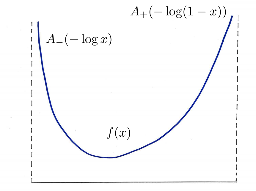
Figure 1. Special representation of an Arnol’d flow.

A motivation to study Arnol’d flows comes from considering smooth area-preserving flows on the torus $\mathbb{T}^{2}$, with the simplest possible critical points, namely a center and a simple saddle (as in Figure 2). These flows are also known as multi-valued or locally Hamiltonian flows (see in particular the works by Novikov and its school [29]) since in suitable coordinates they are locally given by $\stackrel{{\scriptstyle\cdot}}{{x}}=\frac{\partial H}{\partial y}$, $\stackrel{{\scriptstyle\cdot}}{{y}}=-\frac{\partial H}{\partial x}$, where $H$ is a local Hamiltonian. The minimal components of a typical such flow consist of invariant circles (which foliates a neighbourhood of the center, see Figure 2) and a non-trivial minimal component (supported on a torus minus a disk). The restriction $(\phi_{t})$ of the flow to the minimal component admits a special representation of the form described above. All this was first remarked by Arnol’d in the paper [3] (from which the name Arnol’d flows comes), where mixing of $(\phi_{t})$ was conjectured.

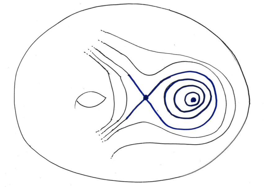
(a) on the torus

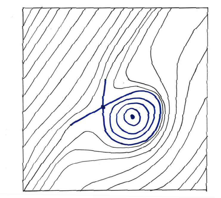
(b) on $\mathbb{R}^{2}/\mathbb{Z}^{2}$

Figure 2. A locally Hamiltonian flow on $\mathbb{T}^{2}$ with a periodic orbits island and a minimal component (Arnol’d flow).

Our next result shows disjointness of rescalings of Arnol’d flows:

Theorem 1.2.

There exists a full Lebesgue measure set $\mathcal{D}\subset\mathbb{T}$ such that for every $\alpha\in\mathcal{D}$ and every $p,q>0$, $\frac{p}{q}\notin\left\{1,\frac{A_{-}}{A_{+}},\frac{A_{+}}{A_{-}}\right\}$, the flows $((R_{\alpha})_{{pt}}^{f})$ and $((R_{\alpha})_{{qt}}^{f})$ are disjoint.

The proof of Theorem 1.2 which is done in Section 7 (and uses the results of Sections 6) is also based on the disjointness criterion given by Theorem 3.1.

Theorems 1.2 and 1.1 show an interesting phenomenon: the Ratner property in the non-homogeneous setting yields stronger dynamical consequences than in the homogeneous one. The reason (which will be explained in more details in Section 5) is that the Ratner property for a horocycle flow (hence in the homogeneous setting) depends only on the distance between the initial points and not on their position in the space. In all other examples of a Ratner property (in particular, for smooth non-trivial time changes of horocycle flows) divergence depends both on their distance and, what is more important, on their position in the space. This allows one to get stronger rigidity conclusions for the set of joinings.

Finally, our third main result, which is once again based on the disjointness criterion given by Theorem 3.1, shows that the two classes of parabolic flows considered so far, namely smooth time changes of horocycle flows and Arnol’d flows, are typically disjoint:

Theorem 1.3.

There exists a full Lebesgue measure set of rotation numbers $\mathcal{D}\subset\mathbb{T}$ such that for every $\alpha\in\mathcal{D}$, every horocycle flow $(h_{t})$ (with $\Gamma$ cocompact) and every $\tau\in C^{1}(M)$, the Arnol’d flow $((R_{\alpha})_{{t}}^{f})$ and the time-change flow $(\widetilde{h}^{\tau}_{t})$ are disjoint.

The proof of Theorem 1.3 is at the heart of Section 8. Notice that since the result holds for all smooth time changes, it implies in particular disjointness between (homogenous) horocycles flows and area-preserving flows in the class of Arnol’d flows considered in Theorem 1.2 (sets $\mathcal{D}$ in both theorems are the same).

Consequences for Möbius disjointness.

We now briefly discuss a relation between Theorems 1.1 and 1.2 with the Möbius disjointness problem [34] which is lately under intensive study, see e.g. survey [11]. If $(T_{t})$ is a continuous flow on a compact metric space $X$ then it is called Möbius disjoint if

(1.2) $$\lim_{N\to\infty}\frac{1}{N}\sum_{n\leqslant N}F(T_{nt}x)\boldsymbol{\mu}(n)=0$$

for all $F\in C(X)$, $t\in\mathbb{R}$ and $x\in X$, where $\boldsymbol{\mu}$ stands for the classical Möbius function (whose definition is recalled in Section 9). Sarnak conjectured in [34] that all zero entropy homeomorphisms are Möbius disjoint. As recent development shows, Sarnak’s conjecture is very likely equivalent to the famous Chowla conjecture on correlations of the Möbius function, see [11] for details.

Möbius disjointness for horocycle flows has been proved by Bourgain, Sarnak and Ziegler in [5]. A few years ago M. Ratner asked about Möbius disjointness of (smooth) time changes of horocycle flows (see Question 7 in [11]). Since the flows appearing in Theorems 1.1 and 1.2 are totally ergodic (in fact, they are known to be mixing, see respectively [35] for Arnol’d flows and [28] for time changes of horocycle flows), in view of the so called Kátai-Bourgain-Sarnak-Ziegler criterion for orthogonality in [5] (recalled in Section 9), our results in particular imply that Möbius disjointness holds for all smooth time-changes in $B^{+}(M)$ of horocycle flows and for all uniquely ergodic models of Arnol’d flows (see Section 9 for more details). In particular, Theorem 1.1 answers positively Ratner’s question on Möbius disjointness (Question 7 in [11]).

A question which has seen a recent surge of interest is uniform convergence in Möbius disjointness, namely whether the convergence in (1.2) is uniform in $x\in{X}$. It is for example shown in [2] that Sarnak’s conjecture is equivalent to its uniform convergence form. While on the level of Möbius disjointness we cannot see any difference between horocycle flows and their (non-trivial) time changes, this situation changes drastically when we ask about uniformity. Indeed, Theorem 1.1 not only answers positively Ratner’s question on Möbius disjointness, but it also yields uniform convergence (in $x\in M$) in (1.2). On the other hand, the question of whether uniform convergence holds for horocycle flows themselves remains largely open, see Question 5 in [11]. Thus, this is another instance, where in the non-homogeneous set up one can prove stronger properties than in the homogeneous world.

In the case of Arnol’d flows and the corresponding locally Hamiltonian flows, however, while we show Möbius disjointness of any uniquely ergodic realization, we have been unable until now to show uniformity of convergence in (1.2). Uniform convergence for Möbius disjointness, especially in its stronger form of so called convergence on (typical) short intervals, will be discussed in some detail in Section 9.

We conclude by saying that the (parabolic) disjointness criterion (Theorem 3.1) seems to be a general tool in studying disjointness of systems with a Ratner property. A variant of this criterion is used in a recent work of G. Forni and the first author [14], where disjointness properties of time changes of Heisenberg nilflows are studied and also in recent works of P. Berk and the first author [4] and C. Dong and the first author [8] for getting disjointness of some classes of interval exchange transformations (IET’s) and translation flows.

Outline of the paper

The structure of the paper is as follows. In Section 2, we recall some basic definitions and properties, in particular about flows and special flows, joinings and irrational rotations on the circle. We also recall, for the convenience of the reader, the definition of the SR-property (a recent variation of the classical Ratner property), which is not directly used, but implicitly drives many of the exploited phenomena. In Section 3, we state and prove the new disjointness criterion (Theorem 3.1). Section 4 is devoted to the proof of Theorem 1.1 on disjointness for time changes of horocycle flows which gives the first illustration of the use of our criterion. In Section 5, we state a disjointness criterion in the language of special flows and we then show how it can be deduced from our main criterion on disjointness. The proof of the disjointness result for Arnol’d flows, i.e. Theorem 1.2, takes Sections 6 and 7: in Sections 6 we first prove some estimates on the growth of Birkhoff sums of derivatives of the roof function, then in Sections 7 we use them in order to quantify shearing and derive the splitting and slow drift of nearby orbits, properties which are needed to apply the disjointness criterion. In Section 8, we show that Arnol’d flows from the considered class are disjoint with smooth time changes of horocycle flows (Theorem 1.3). Finally, in Section 9 we discuss consequences of our main results to the problem of Möbius disjointness. Three appendices follow. In the first two, we give the proofs of two technical results which are used in the proof of Theorem 1.1: in the first one, Appendix A, we prove some quantitative shearing properties for time-changes of horocycle flows; in Appendix B we state a result on ergodic averages of a special family of smooth functions which can be deduced from [6] (we thank G. Forni for the proof). Finally, in Appendix C, we present a missing link in the literature, namely, the equivalence between two different kinds of convergence on short intervals.

2. Preliminaries: definitions, notation and some basic facts

2.1. Flows, joinings and disjointness

Assume that $(Z,\mathcal{D},\kappa)$ is a probability standard Borel space. If $Z$ is additionally a metric space (with a metric $d$), then we will also write $(Z,\mathcal{D},\kappa,d)$ to emphasize the role of $d$. By ${\rm Aut}(Z,\mathcal{D},\kappa)$, we denote the set of all automorphisms of $(Z,\mathcal{D},\kappa)$, i.e. $R\in{\rm Aut}(Z,\mathcal{D},\kappa)$ if $R:Z\to Z$ is a bi-measurable, measure-preserving $\kappa$-a.e. bijection. Each $R\in{\rm Aut}(Z,\mathcal{D},\kappa)$ determines a unitary operator, also denoted by $R$, on $L^{2}(Z,\mathcal{D},\kappa)$ given by $Rf:=f\circ R$ for $f\in L^{2}(Z,\mathcal{D},\kappa)$. Endowed with the weak operator topology of unitary operators, ${\rm Aut}(Z,\mathcal{D},\kappa)$ becomes a Polish group.

We will be mainly deal with flows, i.e. with measurable, measure-preserving $\mathbb{R}$-actions $(R_{t})_{t\in\mathbb{R}}\subset{\rm Aut}(Z,\mathcal{D},\kappa)$. Measurability means that the map $(z,t)\to R_{t}z$ is measurable (in fact, it is equivalent to saying that the unitary representation $t\mapsto R_{t}$ is continuous). If no confusion arises, we will abbreviate notation $(R_{t})_{t\in\mathbb{R}}$ to $R_{t}$. By the centralizer $C(R_{t})$ of the flow $R_{t}$, we mean the set of all $W\in{\rm Aut}(Z,\mathcal{D},\kappa)$ that commute with the flow: $WR_{t}=R_{t}W$ (for each $t\in\mathbb{R}$) (in fact, $C(R_{t})$ is a closed subgroup of ${\rm Aut}(Z,\mathcal{D},\kappa))$. It is well-known (see e.g. [7]) that if a flow $R_{t}$ is ergodic (i.e. its only invariant sets are either of zero or full measure) then for Lebesgue a.e. $s\in\mathbb{R}$, the time automorphism $R_{s}$ is ergodic. Given $0\neq r\in\mathbb{R}$, by $R_{rt}$ we denote the flow $t\mapsto R_{rt}$.

Assume that $T_{t},S_{t}$ are flows on probability standard Borel spaces $(X,\mathcal{B},\mu)$ and $(Y,\mathcal{C},\nu)$, respectively. A joining between $T_{t}$ and $S_{t}$ is a $T_{t}\times S_{t}$-invariant (for each $t\in\mathbb{R}$) probability measure on $(X\times Y,\mathcal{B}\otimes\mathcal{C})$ with the projections $\mu$ and $\nu$, respectively. By $J(T_{t},S_{t})$ we denote the set of joinings between the flows $T_{t}$ and $S_{t}$. Following Furstenberg [17], we say that $T_{t}$ and $S_{t}$ are disjoint, and we write $T_{t}\perp S_{t}$, if product measure $\mu\otimes\nu$ is the only member of $J(T_{t},S_{t})$. Note that if $T_{t}\perp S_{t}$ then at least one of the two flows must be ergodic. If both flows are ergodic, then by $J^{e}(T_{t},S_{t})$ we denote the subset of ergodic joinings, that is, of those $\rho\in J(T_{t},S_{t})$ which make the flow $(T_{t}\times S_{t})_{t\in\mathbb{R}}\subset{\rm Aut}(X\times Y,\mathcal{B}\otimes\mathcal{C},\rho)$ ergodic (this set is always nonempty, as the ergodic decomposition of any joining yields a.e. ergodic component also a joining). Note also that if $W$ yields an isomorphism of $T_{t}$ and $S_{t}$ then the formula

$$\rho(B\times C):=\mu(B\cap W^{-1}C),\;\;B\in\mathcal{B},C\in\mathcal{C},$$

determines a member of $J(T_{t},S_{t})$ which is ergodic if $T_{t}$ (hence $S_{t}$) is ergodic. Note also that, for each $r\neq 0$, we have $J(T_{t},S_{t})=J(T_{rt},S_{rt})$ with the equality $J^{e}(T_{t},S_{t})=J^{e}(T_{rt},S_{rt})$ whenever the flows $T_{t}$ and $S_{t}$ are ergodic.

Unless it is stated otherwise, flows are assumed to be free $\mathbb{R}$-actions, i.e. $t\mapsto T_{t}x$ is 1-1 for $\mu$-a.e. $x\in X$. If $T_{t}$ is ergodic and $S_{t}=Id$ (for each $t\in\mathbb{R}$, so $S_{t}$ is not a free $\mathbb{R}$-action) then $T_{t}\perp S_{t}$. In fact, whenever an automorphism $R\in{\rm Aut}(Z,\mathcal{D},\kappa)$ is ergodic then $R$ is disjoint from the identity (defined on an arbitrary probability, standard Borel space). We recall here that joinings for automorphisms are defined similarly as for flows – we replace $\mathbb{R}$-actions by $\mathbb{Z}$-actions, in fact, joinings can be defined for actions of more general groups, see e.g. [19] for more details.

Remark 2.1.

Although, in general, ergodic properties of a time automorphism and the whole flow are different (e.g. a time automorphism can have more factors, or can have a larger centralizer), there is no difference if we consider disjointness of time automorphisms. More precisely, given $r\neq 0$, the flows $T_{rt}$ and $S_{rt}$ are disjoint if and only if the time automorphisms $T_{r}$ and $S_{r}$ are disjoint. Indeed, the $\mathbb{Z}$-subaction $(T_{rn}\times S_{rn})$ is cocompact, so if $\rho\in J(T_{r},S_{r})$ then $\frac{1}{r}\int_{0}^{r}\rho\circ(T_{s}\times S_{s})\,ds\in J(T_{rt},S_{rt})$.

2.2. Special flows

Assume that $R\in{\rm Aut}(Z,\mathcal{D},\kappa)$ is an ergodic automorphism and let $f:Z\to\mathbb{R}$ belongs to $L^{1}(Z,\mathcal{D},\kappa)$, $f>0$ ($\kappa$-a.e). For $n>0$, set $f^{(n)}(z)=\sum_{j=0}^{n-1}f(R^{j}z)$. Complemented by $f^{(0)}(z)=0$ and $f^{(-n)}(z):=-f^{(n)}(T^{-n}z)$, we obtain the cocycle identity

(2.1) $$f^{(m+n)}(z)=f^{(m)}(z)+f^{(n)}(R^{m}z)$$

true for $\kappa$-a.e. $z\in Z$ and all $m,n\in\mathbb{Z}$. By a special flow $R^{f}=(R^{f})_{t\in\mathbb{R}}$ with the base $R$ and the roof function $f$, we mean the $\mathbb{R}$-action given by

(2.2) $$R^{f}_{t}(z,r)=(R^{n}z,r+t-f^{(n)}(z)),$$

where $n\in\mathbb{Z}$ is the only number satisfying $f^{(n)}(z)\leqslant r+t<f^{(n+1)}(z)$. Then $T^{f}_{t}$ is a flow defined on the probability standard Borel space $(Z^{f},\mathcal{D}^{f},\kappa^{f})$, where the space

$$Z^{f}=\{(z,r)\in Z\times\mathbb{R}:\>z\in Z,0\leqslant r<f(z)\},$$

consists of the area in the plane under the graph of the function $f$, $\mathcal{D}^{f}$ is the restriction of the product $\sigma$-algebra $\mathcal{D}\otimes\mathcal{B}(\mathbb{R})$ to $Z^{f}$, and $\kappa^{f}$ is the restriction of product measure $\kappa\otimes\lambda_{\mathbb{R}}$ to $\mathcal{D}^{f}$, normalized by $\int_{Z}f\,d\kappa$. It is not hard to see that in view of the ergodicity of $R$, the special flow $R^{f}_{t}$ is also ergodic.

Remark 2.2.

One can observe that if $r\neq 0$ then the two special flows

$$\mbox{$(R^{f}_{r^{-1}t})_{t\in\mathbb{R}}$ and $(R^{rf}_{t})_{t\in\mathbb{R}}$ are isomorphic}.$$

Indeed, the map $Z^{f}\ni(x,s)\mapsto(x,rs)\in Z^{rf}$ is measure-preserving and equivariant.

2.3. Time changes of flows

Assume that $R_{t}$ is a flow on $(Z,\mathcal{D},\kappa)$ and let $v\in L^{1}(Z,\mathcal{D},\kappa)$ be a positive function. The function $v$ determines a cocycle over $R_{t}$ (which, by abusing the notation, we will denote again by $v$), given by the formula

(2.3) $$v(t,x):=\int_{0}^{t}v(R_{s}x)ds.$$

Recall that the cocycle property means that $v(t_{1}+t_{2},x)=v(t_{1},x)+v(t_{2},R_{t_{1}}x)$ for $\kappa$-a.e. $x\in{Z}$ and all $t_{1},t_{2}\in\mathbb{R}$. One can then show (see for example [7]) that for a.e. $x\in{Z}$ and all $t\in\mathbb{R}$, there exists a unique $u=u(t,x)$ such that

(2.4) $$\int_{0}^{u}v(R_{s}x)\,ds=t\;\;$$

(Note that if $t<0$, then $u<0$.) Now, we can define $\widetilde{R}_{t}(x):=R_{u(t,x)}(x)$ and this is indeed an $\mathbb{R}$-action as the function $u=u(t,x)$ satisfies the cocycle identity: $u(t_{1}+t_{2},x)=u(t_{1},x)+u(t_{2},\widetilde{R}_{t_{1}}x)$. The new flow $\widetilde{R}_{t}$ has the same orbits as the original flow (hence it is ergodic if $R_{t}$ was), and it preserves the measure $\widetilde{\kappa}\ll\kappa$, where $\frac{d\widetilde{\kappa}}{d\kappa}={v/\int_{Z}v\,d\kappa}$. We will also use notation $\widetilde{R}^{v}_{t}$ for the time change if it is not clear which function $v$ is used.

We say that $v$ is a quasi-coboundary if $v(t,x)=\xi(x)-\xi(R_{t}x)+t$ for a measurable $\xi:Z\to\mathbb{R}$. If $v$ is a quasi-coboundary, then the flows $R_{t}$ and $\widetilde{R}_{t}$ are isomorphic. More generally, if $w:{Z}\to\mathbb{R}^{+}$ is another time change of $R_{t}$ and if

$$v(t,x)-w(t,x)=\xi(x)-\xi(R_{t}x)$$

(for $\kappa$-a.e. $x\in{Z}$ and all $t\in\mathbb{R}$) then the two time changes $\widetilde{R}^{v}_{t}$ and $\widetilde{R}^{w}_{t}$ are isomorphic, where the isomorphism is given by the map $x\mapsto\widetilde{R}^{w}_{\xi(x)}x$ (in the special case of the trivial time change of $R_{t}$ given by $w=1$, for which the associated cocycle is $w(x,t)\equiv t$, this reduces to the previous definition of quasi-coboundary). Note that on $Z$ we consider, in general, two different absolutely continuous measures.

Remark 2.3.

One can show that any special flow $R_{t}^{f}$, where $R\in{\rm Aut}(Z,\mathcal{D},\kappa)$, can be obtained from a time change of the suspension of $R$, i.e. from a time change of the special flow over $R$ built under the constant function 1.

Remark 2.4.

If $R_{t}$ is a smooth flow on a manifold $Z$ and $v$ is also smooth then the time change flow $\widetilde{R}^{v}_{t}$ is a smooth flow. In fact, when $A:Z\to TZ$ is a vector field and

$$\frac{d}{dt}R_{t}x=A(R_{t}x)$$

and if $v:Z\to\mathbb{R}^{+}$ is smooth, then consider the vector field $\frac{1}{v}A$. There is a unique (smooth) flow $\widetilde{R}_{t}$ given by

$$\frac{d}{dt}\widetilde{R}_{t}x=\frac{1}{v(\widetilde{R}_{t}x)}A(\widetilde{R}_{t}x)$$

and one can show that the flow $\widetilde{R}_{t}$ thus defined (which is clearly smooth by construction) coincides with the flow $\widetilde{R}^{v}_{t}$ defined at the beginning of the section.

Let us conclude this section with two very simple lemmas on time changes which will be helpful later.

Lemma 2.1.

Assume that $Z$ is a compact metric space and $R_{t}:Z\to Z$ is a uniquely ergodic flow. Then, for any $v\in C(Z)$ a positive function with $\int_{Z}v\,d\kappa=1$, we have

$$\lim_{t\to\infty}\frac{t}{u(t,z)}=1$$

uniformly in $z\in Z$.

Proof.

Remark that for each (and, in fact, uniformly in) $z\in Z$, we have

$$\frac{t}{u(t,z)}=\frac{1}{u(t,z)}\int_{0}^{u(t,z)}v(R_{s}z)\,ds\xrightarrow[t\to\infty]{}\int_{Z}v\,d\kappa=1.$$

The conclusion follows immediately. ∎

The following shows that the study of rescalings of a flow can be reduced to the study of time changes.

Lemma 2.2.

Consider a flow $R_{t}:Z\to Z$ on $(Z,\mathcal{D},\kappa)$, $v:Z\to\mathbb{R}^{+}$ integrable and let $\widetilde{R}^{v}_{t}$ be the corresponding time change. Fix $0<p\in\mathbb{R}$ and consider $\widetilde{R}^{pv}_{t}$. Then, for $\kappa$-a.e. $x\in Z$ and all $t\in\mathbb{R}$, we have

$$\widetilde{R}^{pv}_{t}(x)=\widetilde{R}^{v}_{(1/p)t}(x).$$

Proof.

For $\kappa$-a.e. $x\in Z$ and all $t\in\mathbb{R}$ we have $\int_{0}^{u(x,t)}(pv)(R_{s}x)\,ds=pt$. This can be interpreted by saying that $\widetilde{R}^{pv}_{pt}(x)=R_{u(x,t)}(x)$. Hence, since $R_{u(x,t)}(x)=\widetilde{R}_{t}(x)$, it gives the conclusion. ∎

2.4. Irrational rotations, Denjoy-Koksma inequality

For each $x\in\mathbb{R}$, we set

$$\|x\|:=\min(\{x\},1-\{x\}),\qquad\text{where}\ \{x\}=x-[x]$$

stands for the fractional part of $x$. By $\mathbb{T}=[0,1)$ we denote the additive circle. Then, clearly, $\|\cdot\|$ determines a translation invariant metric on $\mathbb{T}$. By $\lambda_{\mathbb{T}}$ (or $\lambda$) we will denote Lebesgue measure on $\mathbb{T}$.

Let

$$[0,1)\ni\alpha=[0;a_{1},a_{2},\ldots]=\frac{1}{a_{1}+\frac{1}{a_{2}+\ldots}}$$

be irrational. Then the positive integers $a_{i}$ are called partial quotients of $\alpha$. By setting

$$p_{0}=0,p_{1}=1,p_{n+1}=a_{n+1}p_{n}+p_{n-1},\;q_{0}=1,q_{1}=a_{1},q_{n+1}=a_{n+1}q_{n+1}+q_{n-1}$$

for $n\geqslant 2$, we obtain the sequences $(p_{n}),(q_{n})$ of numerators and denominators of $\alpha$, respectively. Then (see e.g. [23])

$$\frac{1}{2q_{n}q_{n+1}}<\left|\alpha-\frac{p_{n}}{q_{n}}\right|<\frac{1}{q_{n}q_{n+1}};$$

equivalently,

(2.5) $$\frac{1}{2q_{n+1}}<\|q_{n}\alpha\|<\frac{1}{q_{n+1}}.$$

From this inequality, we can deduce the following elementary spacing properties of orbits which we will use several times later.

Lemma 2.3 (Spacing of orbits up to return times).

For any $x\in\mathbb{T}$ and $n\in\mathbb{N}$, the orbit $\{x+i\alpha,\ 0\leqslant i<q_{n}\}$ is such that

(2.6) $$\|x+i\alpha-(x+j\alpha)\|\geqslant\frac{1}{2q_{n}},\qquad\text{for\ all}\ 0\leqslant i\neq j<q_{n}.$$

On the other hand, in each interval of length $2/q_{n}$ there must be a point of the form $x+j\alpha$ for some $0\leqslant j<q_{n}$.

Proof.

For the first part, note that for $0\leqslant i,j<q_{n}$, $\|x+i\alpha-(x+j\alpha)\|=\|(i-j)\alpha\|$ with $|i-j|<q_{n}$. Since $\frac{1}{2q_{n}}<\|q_{n-1}\alpha\|$ and $\|r\alpha\|\geqslant\|q_{n-1}\alpha\|$ whenever $|r|<q_{n}$, we have (2.6). For the second, assuming that $\alpha>\frac{p_{n}}{q_{n}}$, we have $k\alpha-\frac{kp_{n}}{q_{n}}<\frac{1}{q_{n+1}}$ for $0\leqslant k<q_{n}$, so that in particular there exist $0\leqslant i\neq j<q_{n}$ such that

$$\|x+i\alpha-(x+j\alpha)\|<\frac{1}{q_{n}}+\frac{1}{q_{n+1}}<\frac{2}{q_{n}}.$$

Treating the case $\alpha<\frac{p_{n}}{q_{n}}$ similarly, the second part follows. ∎

If $f:\mathbb{T}\to\mathbb{R}$ has bounded variation then, for each $n\geqslant 0$ and $x\in\mathbb{T}$, we have the following Denjoy-Koksma inequality:

(2.7) $$\left|f^{(q_{n})}(x)-q_{n}\int_{\mathbb{T}}f\,d\lambda\right|\leqslant 2{\rm Var}(f),$$

see e.g. [25].

We will also make use of so called Ostrowski expansion of a natural number $N$. Namely, we can represent $N$ as

$$N=\sum_{j=1}^{K}b_{j}q_{j},$$

where $0\leqslant b_{j}\leqslant a_{j}$ (and $b_{K}\neq 0$) and if, for some $j$, we have $b_{j}=a_{j}$ then necessarily $b_{j+1}=0$. Such a decomposition is unique, see e.g. [25].

2.5. Ratner properties

Our main disjointness criterion (Theorem 3.1) is based on quantitative divergence properties and is inspired by the Ratner property (originally defined in [30]) and in particular its recent variation known as the switchable Ratner property (SR-property), first introduced in [10]. While the SR-property is not explicitly used in the paper, it is implicitly present, both in formulation of the disjointness criterion and the phenomena driving it. We hence include in this section its formal definition followed by some explanations, as we think that the reader who is not familiar with it, might benefit by reading it before the following section.

Let $(X,d)$ be a $\sigma$-compact metric space, $\mathcal{B}$ the $\sigma$-algebra of Borel subsets of $X$ and $\mu$ a Borel probability measure on $X$. Let $(T_{t})_{t\in\mathbb{R}}$ be an ergodic flow acting on $(X,\mathcal{B},\mu)$. The Ratner property encodes a quantitative property of controlled divergence of nearby trajectories in the flow direction. Heuristically, we want that for most pairs of nearby points $x,x^{\prime}$, the orbits of $x,x^{\prime}$ split in the flow direction (say at time $t=M$) by a definite amount (the shift $p$, which belongs to a fixed compact set $P$) and then realign, so that now $T_{t}(x)$ and the time-shifted orbit $T_{t+p}(x^{\prime})$ are close, and stay close for a fixed proportion $\kappa M$ of the time it took to see the shift, namely for most times $t\in[M,M+L]$ where $L>\kappa M$ (this is made precise in Definition 2.1). One can see that this type of phenomenon is possible only for parabolic systems, in which orbits of nearby points diverge with polynomial or subpolynomial speed.

In the switchable variation, this phenomenon might not happen for positive times $t$ (i.e. in the future), but only in the past, i.e. for $t<0$ (and one can switch between exploiting the past or the future according to the pair of points $x,x^{\prime}$). This is encoded by the following formal definition. (We comment below on the relation with the definitions in the literature, see Remark 2.5).

Definition 2.1 (SR-property).

We say that the flow $(T_{t})$ has the SR-property (with shifts set $P$) if there exists a compact set $P\subset\mathbb{R}\setminus\{0\}$ (the shifts set) such that:

for every $\varepsilon>0$ and $N\in\mathbb{N}$ there exist $\kappa=\kappa(\varepsilon)$, $\delta=\delta(\varepsilon,N)$ and a set $Z=Z(\varepsilon,N)$ with $\mu(Z)>1-\varepsilon$, such that:

for every $x,y\in Z$ with $d(x,y)<\delta$ and $x$ not in the orbit of $y$, there exist $p=p(x,y)\in P$ and $M=M(x,y),$ $L=L(x,y)$ such that $M\geqslant N$ and ${L}\geqslant\kappa M$, and at least one of the following holds:

1. $d(T_{t}(x),T_{t+p}(y))<\varepsilon\quad\text{for}\quad t\in U\subset[M,M+L]$, or

2. $d(T_{t}(x),T_{t+p}(y))<\varepsilon\quad\text{for}\quad-t\in U\subset[M,M+L]$,

where $U\subset[M,M+L]$ is such that its Lebesgue measure $|U|$ satisfies $|U|>(1-\varepsilon)L$.

Referring to the heuristic explanation before the definition, most initial points is formalized by the set $Z$ of arbitrarily large measure. The splitting and realignement with shift of nearby orbits should happen for arbitrarily large times (i.e. for every $N\geqslant 0$ there must be an $M\geqslant N$). Finally, $(i)$ describes controlled splitting in the future, while $(ii)$ describes controlled splitting in the past.

Remark 2.5.

In the classical Ratner property, $P=\{1,-1\}$ and for all $x,y\in Z$ (i) has to be satisfied. The first extensions of the Ratner property were introduced by K. Fraczek and M. Lemańczyk in [15] and [16] (as mentioned in the introduction) and amounted to allow $P$ to be any finite set (the finite Ratner property) or any compact set $P\subset\mathbb{R}\setminus\{0\}$ (the weak Ratner property). The switchable variation (where the possibility $(ii)$ of controlled splitting in the past is also allowed) was introduced by B. Fayad and the first author in [10].

All the variants of the Ratner properties are defined so that, if $(T_{t})$ has the SR-property, then it has the finite extension of joinings property (shortened as FEJ property, see [10]), which is a rigidity property that restricts the type of self-joinings that $(T_{t})$ can have (see [33, 15]).

3. A criterion for disjointness

The main result of this section is the new disjointness criterion which the main results of the rest of the paper are based on. Since this criterion and the explanations in this section are inspired by the SR-property (even if the property is not used directly), the reader who is not familiar with it might benefit from reading Section 2.5 first.

The statement of the criterion is given in Section 3.2. Since it is rather technical, let us first explain the guiding ideas behind it. The criterion was devised and formulated so that it can be applied to prove disjointness of two flows which both have the SR-property (see Definition 2.1), so that in both flows one can observe a controlled form of divergence of nearby trajectories (for example polynomial divergence), but the speed of divergence for the two flows is different (for example for one flow is it linear, in the other quadratic).

The key shearing phenomenon exploited in the criterion is that, for pairs of two nearby points in the first system and two nearby points in the second, after some time (depending on both pairs of points) we will see a relative divergence, i. e. in one pair we will see a realignement with some shift $C_{1}>0$ in the flow direction, while in the other we will see a realignement with a shift $C_{2}>0$ with $C_{1}\neq C_{2}$. To see that this is the case when both flows have the Ratner property (not switchable for now) but with different speeds, one can reason as follows. Using the Ratner or SR-property, one can find times $M_{1}>0$ and $M_{2}>0$ such that the first pair splits exactly by $1$ at time $M_{1}$ and the second splits by exactly $1$ at time $M_{2}$. If the second pair has not yet not split at time $M_{1}$ (or symmetrically, first pair has not yet split at time $M_{2}$), then we are done with $C_{1}=1$ for one flow and $C_{2}=0$ for the other. The interesting case is when $M_{1}$ and $M_{2}$ are very close (assume for simplicity that $M_{1}=M_{2}$). In this case one can use the fact that the speed of divergence is different to conclude that after some time, say $10M_{1}$, the two pairs will have split by a different amount (in the linear and quadratic case, it is a simple consequence of the fact that a line and parabola can have at most two points of intersection -at time $M_{1}$- and after $M_{1}$ they start slowly diverging). This explains how the relative shearing appears in this situation.

Let us remark that if both flows have only the switchable Ratner property, one might have pairs of points for which one see the Ratner form of shearing only in the past for one flow, and only in the future for the other. Therefore, there is no hope to implement the heuristic described above on the whole (or large parts) of the space. An essential feature of the criterion is that for one of the two flows one can consider only pairs of points in small parts of space (whose measure is bounded from below, but not necessarily close to one), on which one sees controlled shearing both forward and backward. Thus, one can couple these pairs with pairs in the other flow which have the Ratner property in the future or the past to get the relative divergence explained above. We will come back to this point after the statement of the criterion in Section 3.2.

In order to give the precise formulation of the criterion, we now first need to give the definition of almost linear reparametrization.

3.1. Almost linear reparametrizations

In the disjointness criterion stated in the next Section 3.2, we will consider a class of time reparametrizations given by functions $t\mapsto a(t)$ which are almost linear (in the sense of Definition 3.1). Heuristically, we want the function $a(\cdot)$ to be "close" to a linear function, either being close to a piecewise linear function, which on each interval of continuity has the form $a(t)=t+R_{i}$ (we call this case (PAL) for Piecewise Almost Linear), or having derivative $a^{\prime}(t)$ close to $1$ (a case dabbed (SAL), for Smoothly Almost Linear).

For a (measurable) set $I\subset\mathbb{R}$, $|I|$ denotes its Lebesgue measure.

Definition 3.1 (almost linear functions and good triples).

Assume that $I=[u_{1},u_{2}]$ is an interval, $a:I\to\mathbb{R}$, $U\subset I$ and $0<d,\xi<1$. We say that $a$ is almost linear and that the triple $(a,U,d)$ is $\xi$-good if at least one of the following holds:

1. (Piecewise Almost Linear function) we can write $U$ as $U=\bigcup_{i=1}^{v}(c_{i},d_{i})$, where $v\leqslant|I|/d$ and $|U|>(1-\xi)|I|$, and for each $i=1,\ldots,v$, for $x\in(c_{i},d_{i})$ we have that $a(t)=t+R_{i}$ for some $R_{i}\in\mathbb{R}$ such that

   $$R_{1}\leqslant\xi|I|,\qquad|R_{i+1}-R_{i}|<\xi\text{ for every }i=1,\ldots,v-1.$$

   In this case we say that $a$ is a piecewise almost linear function.

2. (Smooth Almost Linear function) the function $a\in C^{1}(I)$, $U=I=[u_{1},u_{2}]$ and we have that $|a(u_{i})-u_{i}|\leqslant\xi|I|$ for $i=1,2$ and

   $$1-\xi<a^{\prime}(t)\leqslant 1+\xi,\qquad\text{for\ every}\ t\in I.$$

   In this case we say that $a$ is a smooth almost linear function.

Remark 3.1.

The notion of (PAL) for $a(\cdot)$ is introduced in order to deal with special flows: in this case, we need to take care of the fact that special flows are discontinuous close to the roof. This phenomenon produces the decomposition $(c_{i},d_{i})$, $i=1,\ldots,v$ in (PAL).

This definition of almost linear functions and good triples is given so that the following result (which is essentially based on a change of variables argument) holds. The lemma guarantees that if $a(\cdot)$ is (PAL) or (SAL) then the orbital integrals $\int_{M}^{M+L}f(T_{t}x)dt$ and $\int_{M}^{M+L}f(T_{a(t)}x)dt$ are close.

Lemma 3.1 (Closeness of almost linear good reparametrizations).

Let $0<d,\xi<1$, $a:[M,M+L]\to\mathbb{R}$ and let $U\subset[M,M+L]$ be such that $a$ is almost linear and $(a,U,d)$ is $\xi$-good. Assume that $f:\mathbb{R}\to(0,1]$ is measurable. Then

$$\frac{1}{L}\int_{M}^{M+L}f(a(t))\,dt<\frac{1}{L}\int_{M}^{M+L}f(s)\,ds+9\xi/d.$$

The rest of this subsection will be taken by the proof of this lemma.

Proof.

Assume first that $a$ is smoothly almost linear, that is, (SAL) is satisfied. Then

$$\left|\frac{1}{L}\int_{M}^{M+L}f(a(t))\,dt-\frac{1}{L}\int_{M}^{M+L}f(a(t))a^{\prime}(t)\,dt\right|\leqslant\xi.$$

On the other hand, substituting $s=a(t)$, by the assumptions on the endpoints given by $(SAL)$, we obtain that

$$\frac{1}{L}\int_{M}^{M+L}f(a(t))a^{\prime}(t)\,dt=\frac{1}{L}\int_{a(M)}^{a(M+L)}f(s)\,ds=\frac{1}{L}\int_{M}^{M+L}f(s)\,ds+2\xi.$$

Combining the estimates, this concludes the proof in this case (since $d<1$ and hence $3\xi<9\xi/d$).

Assume now that $a$ is piecewise almost linear, so (PAL) is satisfied. Let $A_{s}:=\{1\leqslant i\leqslant v\;:\;d_{i}-c_{i}\leqslant\xi\}$ (where $s$ stays for short intervals). Let $U_{s}:=\bigcup_{i\in A_{s}}[c_{i},d_{i}]$ and $U_{l}:=U\setminus U_{s}$ (where $l$ stays for large). We then have

$$\left|\frac{1}{L}\int_{M}^{M+L}f(a(t))\,dt-\frac{1}{L}\int_{U_{l}}f(a(t))\,dt\right| =\frac{1}{L}\int_{(I\backslash U)\bigcup U_{s}}f(a(t))\,dt$$

$$\leqslant\frac{|I\backslash U|}{L}+\frac{\xi v}{L}\leqslant\frac{\xi L}{L}+\frac{\xi}{L}\frac{L}{d}<\frac{2\xi}{d}$$

(where in the last inequality we used that $d<1$). Moreover, substituting ${r}=a(t)$ on each $(c_{i},d_{i})$ for $i\notin A_{s}$ and denoting by $a(x^{\pm})$ respectively the right and left limit of the function $a(t)$ as $t\to x^{\pm}$, we get

$$\frac{1}{L}\int_{U_{l}}f(a(t))\,dt =\frac{1}{L}\displaystyle\sum_{\begin{subarray}{c}i=1,\dots,v\\ i\notin A_{s}\end{subarray}}\int_{a(c_{i}^{+})}^{a(d_{i}^{-})}f({r})\,d{r}$$

(3.1) $$=\frac{1}{L}\displaystyle\sum_{\begin{subarray}{c}i=1,\dots,v\\ i\notin A_{s}\end{subarray}}\int_{a(c_{i}^{+})}^{a(d_{i}^{-})-\xi}f({r})\,d{r}+\frac{1}{L}\displaystyle\sum_{\begin{subarray}{c}i=1,\dots,v\\ i\notin A_{s}\end{subarray}}\int_{a(d_{i}^{-})-\xi}^{a(d_{i}^{-})}f({r})\,d{r}.$$

Since $|A_{s}|\leqslant v\leqslant L/d$ (where $|A_{s}|$ denotes the cardinality of $A_{s}$), we have

$$\frac{1}{L}\displaystyle\sum_{\begin{subarray}{c}i=1,\dots,\\ vi\notin A_{s}\end{subarray}}\int_{a(d_{i}^{-})-\xi}^{a(d_{i}^{-})}f({r})\,d{r}\leqslant\frac{\xi|A_{s}|}{L}\leqslant\frac{\xi}{d}.$$

Now, we estimate the first term in RHS of (3.1). We claim that the intervals $[a(c_{i}^{+}),a(d_{i}^{-})-\xi]$ for $i\notin A_{s}$ are non-empty (since $i\notin A_{s}$ implies that $d_{i}-c_{i}>\xi$ and hence $a(d_{i}^{-})-a(c_{i}^{+})>\xi$) and pairwise disjoint. To see this, notice that by the definition (PAL) of almost linear function, for $i\notin A_{s}$, we have

$$a(c_{i}^{+})=c_{i}+R_{i}\leqslant d_{i}+R_{i}-\xi=a(d_{i}^{-})-\xi=d_{i}+R_{i}-\xi\leqslant c_{i+1}+R_{i+1}=a(c_{i+1}^{+}),$$

which proves that the intervals $[a(c_{i}^{+}),a(d_{i}^{-})-\xi]$ are pairwise disjoint (and in increasing order). This now gives that

$$\frac{1}{L}\sum_{i=1,i\notin A_{s}}^{v}\int_{a(c_{i}^{+})}^{a(d_{i}^{-})-\xi}f({r})\,d{r}\leqslant\frac{1}{L}\int_{a(c_{1}^{+})}^{a(d_{v}^{-})}f({r})\,d{r}.$$

Remark now that, by the assumptions in (PAL) and recalling that $d<1$, we have that

$$|R_{v}|=\left|\sum_{i=1}^{v-1}(R_{i+1}-R_{i})+R_{1}\right|\leqslant\xi v+\xi L\leqslant 2\xi\frac{L}{d}.$$

Hence, using this bound on $R_{v}$ and the assumptions in (PAL) (and $d<1$), we have that

$$\left|\frac{1}{L}\int_{a(c_{1}^{+})}^{a(d_{v}^{-})}f({r})\,d{r}-\frac{1}{L}\int_{M}^{M+L}f({r})\,d{r}\right|\leqslant\frac{|a(c_{1}^{+})-M|+|a(d_{v}^{-})-M-L|}{L}$$

$$\qquad\leqslant\frac{|c_{1}-M|+|d_{v}-M-L|+|R_{1}|+|R_{v}|}{L}\leqslant 3\xi+2\frac{\xi}{d}.$$

Combining all the estimates together, we get the desired conclusion also in this case. This finishes the proof. ∎

3.2. The disjointness criterion

Recall that we are considering measurable, measure-preserving $\mathbb{R}$-actions (i.e. flows) on probability standard Borel spaces. In fact, we will be constantly assuming that our configuration spaces are $\sigma$-compact metric spaces (considered with the Borel $\sigma$-algebras and probability Borel measures).

Let $(T_{t})$ and $(S_{t})$ be two weakly mixing flows acting on $(X,\mathcal{B},\mu,d_{1})$ and $(Y,\mathcal{C},\nu,d_{2})$, respectively. Given $A\subset X$, we set $V^{1}_{\epsilon}(A):=\{x\in X:d_{1}(x,A)<\epsilon\}$, and a similar notation $V^{2}_{\epsilon}(A^{\prime})$ is used for a subset $A^{\prime}$ of $Y$. Let $P=\{p,-p\}$, $p\neq 0$.

Let us first state the criterion, then make some comments that connect it to the heuristics presented at the beginning of the section.

Theorem 3.1 (Disjointness criterion).

Let $0<c<1$. Assume that we have a sequence of sets

$$(X_{k})\subset\mathcal{B},\qquad\mu(X_{k})\to\mu(X),$$

together with a sequence of automorphisms

$$(A_{k})\subset Aut(X_{k},\mathcal{B}|_{X_{k}},\mu|_{X_{k}}),\qquad\text{such that}\ A_{k}\to Id\ \text{uniformly}.$$

Assume moreover that for every $0<\epsilon<1$ and $N\in\mathbb{N}$ there exist a sequence

$$(E_{k})=(E_{k}(\epsilon))\subset\mathcal{B},\qquad\mu(E_{k})\geqslant c\mu(X),$$

and $0<\kappa=\kappa(\epsilon)<\epsilon$, $\delta=\delta(\epsilon,N)>0$ and a set

$$Z=Z(\epsilon,N)\subset Y,\qquad\nu(Z)\geqslant(1-\epsilon)\nu(Y)$$

such that for all $y,y^{\prime}\in Z$ satisfying $d_{2}(y,y^{\prime})<\delta$, every $k$ such that $d_{1}(A_{k},Id)<\delta$ and every $x\in E_{k}\cap X_{k}$, $x^{\prime}:=A_{k}x$ there are

$$M\geqslant N,\qquad L\geqslant 1,\qquad\frac{L}{M}\geqslant\kappa,\quad\text{and}\quad p\in P$$

for which at least one of the following holds:

(3.2) $$\max\left(d_{1}(T_{t}x,T_{a(t)+p}x^{\prime}),\;d_{2}(S_{t}y,S_{a(t)}y^{\prime})\right)<\epsilon\text{ for }t\in U\subset[M,M+L]$$

or

(3.3) $$\max\left(d_{1}(T_{t}x,T_{a(t)+p}x^{\prime}),d_{2}(S_{t}y,S_{a(t)}y^{\prime})\right)<\epsilon\text{ for }-t\in U\subset[M,M+L],$$

where $a:=a_{x,x^{\prime},y,y^{\prime}}:[M,M+L]\to\mathbb{R}$ is extended by $a(-t)=a(t)$, and $(a,U,c)$ is $\epsilon$-good.

Then, the flows $(T_{t})$ and $(S_{t})$ are disjoint.

As we explained at the beginning of this section, the criterion is meant to be applied to two flows having the SR-property (or the Ratner property) but with different speed. The parameters $(X_{k},A_{k},E_{k})$ allows us to relax the SR-property for one of the flows: we only need to control a positive proportion of space (the sets $E_{k}$) and only in a favorite direction (that we control well, for instance, the geodesic direction $A_{k}=g_{1/k}$ for the horocycle flow), we do not need to control all nearby points. The set $Z$ is just the set, where the SR-property holds for the other flow. The almost linear function $a(t)$ describes the relative drift between points $x,x^{\prime}$ (or $y,y^{\prime}$) (for example, it would be $t+td(x,x^{\prime})$ if the divergence is linear). Formulas (3.2) and (3.3) then describe the relative shearing, either in the future or in the past.

The rest of this section is devoted to the proof of the disjointness criterion.

Proof.

Let $\rho\in J((T_{t})_{t\in\mathbb{R}},(S_{t})_{t\in\mathbb{R}})$ be an ergodic joining, $\rho\neq\mu\times\nu$. Recall that by the weak mixing of the flow, all non-zero time automorphisms are weakly mixing, hence ergodic and therefore disjoint from the identity. Thus, since $T_{w}$ is disjoint from $Id$ for $w\in P=\{p,-p\}$ and $\rho$ is not product measure, there exist $B_{w}\in\mathcal{B},C_{w}\in\mathcal{C}$ such that

(3.4) $$|\rho(T_{-w}(B_{w})\times C_{w})-\rho(B_{w}\times C_{w})|>\eta$$

for some $0<\eta<1$. There exists $0<\epsilon<\frac{c\eta}{1000}$ such that

$$\max\left(\left|\mu(V^{1}_{\epsilon}(B_{w}))-\mu(B_{w})\right|,\left|\nu(V^{2}_{\epsilon}(C_{w}))-\nu(C_{w})\right|\right)<\eta/32.$$

Since $\rho$ is a joining, by the triangle inequality, for each $t\in\mathbb{R}$, we have

(3.5) $$|\rho(T_{-t}V^{1}_{\epsilon}(B_{w})\times V^{2}_{\epsilon}(C_{w}))-\rho(T_{-t}B_{w}\times C_{w})|<\frac{\eta}{16}.$$

By applying the pointwise ergodic theorem to the joining flow $(T_{t}\times S_{t},\rho)$ and the sets $T_{-w}B_{w}\times C_{w}$ and $T_{-w}V^{1}_{\epsilon}(B_{w})\times V^{2}_{\epsilon}(C_{w})$ for $w\in P$, there exist $N_{0}\in\mathbb{N}$, $\kappa>0$ (which we can assume additionally to be of the form $\kappa=\kappa(\varepsilon)$ as in the assumptions of our theorem) and a set $U_{1}\in\mathcal{B}\otimes\mathcal{C}$ with $\rho(U_{1})>(1-\frac{c}{100})\rho(X\times Y)$ (recall that $c$ comes from our assumption) such that for every $L,M\geqslant N_{0}$ with $\frac{L}{M}\geqslant\kappa$ and $w\in P\cup\{0\}$, we have

(3.6) $$\left|\frac{1}{L}\int_{M}^{M+L}\mathbbm{1}_{T_{-w}B_{w}\times C_{w}}(T_{t}x,S_{t}y)\,dt-\rho(T_{-w}B_{w}\times C_{w})\right|<\frac{\eta}{16},$$

(3.7) $$\left|\frac{1}{L}\int_{M}^{M+L}\mathbbm{1}_{T_{-w}V^{1}_{\epsilon}(B_{w})\times V^{2}_{\epsilon}(C_{w})}(T_{t}x,S_{t}y)\,dt-\rho(T_{-w}V^{1}_{\epsilon}(B_{w})\times V^{2}_{\epsilon}(C_{w}))\right|<\frac{\eta}{16}$$

and

(3.8) $$\left|\frac{1}{L}\int_{M}^{M+L}\mathbbm{1}_{T_{-w}B_{w}\times C_{w}}(T_{-t}x,S_{-t}y)\,dt-\rho(T_{-w}B_{w}\times C_{w})\right|<\frac{\eta}{16},$$

(3.9) $$\left|\frac{1}{L}\int_{M}^{M+L}\mathbbm{1}_{T_{-w}V^{1}_{\epsilon}(B_{w})\times V^{2}_{\epsilon}(C_{w})}(T_{-t}x,S_{-t}y)\,dt-\rho(T_{-w}V^{1}_{\epsilon}(B_{w})\times V^{2}_{\epsilon}(C_{w}))\right|<\frac{\eta}{16}$$

whenever $(x,y)\in U_{1}$. Let $U_{2}:=U_{1}\cap(X\times Z)$, where $Z=Z(\epsilon,N_{0})$ comes from our assumptions. Then $\rho(U_{2})>(1-c/50)\rho(X\times Y)$. Note also that since $X\times Y$ is $\sigma$-compact, measure $\rho$ is regular and hence, we can additionally assume that $U_{2}$ is compact. Define ${\rm proj}:X\times Y\to X$, ${\rm proj}(x,y)=x$. Then the fibers of ${\rm proj}$ are $\sigma$-compact, and since $U_{2}$ is compact, the fibers of the map ${\rm proj}|_{U_{2}}:U_{2}\to{\rm proj}(U_{2})\subset X$ are also $\sigma$-compact and ${\rm proj}(U_{2})$ is also compact. Thus, by Kunugui’s selection theorem (see e.g. [18], Thm. 4.1), it follows that there exists a measurable (selection) $y:{\rm proj}(U_{2})\to X\times Y$ such that $(x,y(x))\in U_{2}$. Note that $\mu({\rm proj}(U_{2}))\geqslant\rho(U_{2})>(1-c/50)\mu(X)$. By Luzin’s theorem there exists $X_{\rm cont}\subset{\rm proj}(U_{2})$, $\mu(X_{\rm cont})\geqslant(1-c/50)\mu(X)$ such that $y$ is uniformly continuous on $X_{\rm cont}$. Finally, set

$$\widetilde{U}:=U_{2}\cap(X_{\rm cont}\times Y).$$

We have $\rho(\widetilde{U})>(1-c/10)\rho(X\times Y)$. Moreover, if $U_{X}:={\rm proj}(\widetilde{U})$ then also $\mu(U_{X})\geqslant\rho(\widetilde{U})>(1-c/10)\rho(X\times Y)$. Hence, by the definitions of sequences $(A_{k})$ and $(E_{k})=(E_{k}(\epsilon))$, it follows that there exists $k_{0}=k_{0}(\epsilon)$ such that for $k\geqslant k_{0}$, we have

(3.10) $$\mu(A_{-k}(U_{X}\cap X_{k})\cap(U_{X}\cap X_{k})\cap E_{k})>0.$$

Let $\delta=\delta(\epsilon,N_{0})$ come from the assumptions of our theorem. By the uniform continuity of $y:X_{\rm cont}\to Y$ it follows that there exists $0<\delta^{\prime}<\delta$ such that $d_{1}(x_{1},x_{2})<\delta^{\prime}$ implies $d_{2}(y(x_{1}),y(x_{2}))<\delta$ for each $x_{1},x_{2}\in X_{\rm cont}$. Since $A_{k}\to Id$ uniformly and $\widetilde{U}\subset X_{\rm cont}\times Y$, there exists $k_{1}=k_{1}(\epsilon)$ such that for $k\geqslant k_{1}$, $d_{2}(y(x),y(A_{k}x))<\delta$ for $x\in X_{k}\cap X_{\rm cont}$. Fix $k\geqslant\max(k_{0},k_{1}+1)$ (so that $d_{1}(A_{k},Id)<\delta^{\prime}$). Let $x\in A_{-k}(U_{X}\cap X_{k})\cap(U_{X}\cap X_{k})\cap E_{k}$. Such a point does exist in view of (3.10). Set $x^{\prime}=A_{k}x$, $y=y(x)$, $y^{\prime}=y(x^{\prime})$. By definition, $(x,y),(x^{\prime},y^{\prime})\in\widetilde{U}$ and $d_{2}(y,y^{\prime})<\delta$ and all other assumptions of our theorem are satisfied for $(x,y)$, $(x^{\prime},y^{\prime})$ (so that we obtain $M,L,p$ depending on $(x,y)$ and $(x^{\prime},y^{\prime})$ satisfying (3.2) or (3.3)).

We will assume that (3.2) holds and will get a contradiction using (3.6) and (3.7). If (3.3) holds, we argue analogously using (3.8) and (3.9). We claim that

(3.11) $$\rho(T_{-w}(B_{w})\times C_{w})>\rho(B_{w}\times C_{w})-\frac{\eta}{2}.$$

Indeed, in view of (3.5), (3.11) follows by showing that

$$\rho(T_{-w}(V^{1}_{\epsilon}(B_{w}))\times V^{2}_{\epsilon}(C_{w}))>\rho(B_{w}\times C_{w})-\frac{\eta}{4}.$$

Using (3.2) (for $w=p$), (3.6) (for $w=0$) and $(x,y)\in\widetilde{U}\subset U_{1}$ (and remembering that for $U$ in (3.2), we have $|U|>(1-\epsilon)L$ as $(a,U,c)$ is $\epsilon$-good), we obtain that

(3.12) $$\frac{1}{L}\int_{M}^{M+L}\mathbbm{1}_{V^{1}_{\epsilon}(B_{w})\times V^{2}_{\epsilon}(C_{w})}(T_{a(t)+w}x^{\prime},S_{a(t)}y^{\prime})\,dt>\frac{1}{L}\int_{M}^{M+L}\mathbbm{1}_{B_{w}\times C_{w}}(T_{t}x,S_{t}y)\,dt>\\ \rho(B_{w}\times C_{w})-\epsilon-\frac{\eta}{16}.$$

Hence to complete the proof of claim (3.11), it is enough to show that

(3.13) $$\frac{1}{L}\int_{M}^{M+L}\mathbbm{1}_{V^{1}_{\epsilon}(B_{w})\times V^{2}_{\epsilon}(C_{w})}(T_{a(t)+w}x,S_{a(t)}y)\,dt<\rho(T_{-w}V^{1}_{\epsilon}(B_{w})\times V^{2}_{\epsilon}(C_{w}))+\frac{\eta}{8}.$$

Since $(a,U,c)$ is $\epsilon$-good, we get by Remark 3.1 (for $f(t)=\mathbbm{1}_{V^{1}_{\epsilon}(B_{w})\times V^{2}_{\epsilon}(C_{w})}(T_{t+w}x,S_{t}y)$)

$$\frac{1}{L}\int_{M}^{M+L}\mathbbm{1}_{V^{1}_{\epsilon}(B_{w})\times V^{2}_{\epsilon}(C_{w})}(T_{a(t)+w}x,S_{a(t)}y)\,dt\leqslant\\ \frac{1}{L}\int_{M}^{M+L}\mathbbm{1}_{V^{1}_{\epsilon}(B_{w})\times V^{2}_{\epsilon}(C_{w})}(T_{s+w}x,S_{s}y)\,ds+9\epsilon/c\leqslant\\ \rho(T_{-w}V^{1}_{\epsilon}(B_{w})\times V^{2}_{\epsilon}(C_{w}))+\eta/16+9\epsilon/c,$$

where the latter inequality follows from (3.7) for $w\in P$ remembering that $(x,y)\in\widetilde{U}\subset U_{1}$. This completes the proof of (3.13) and hence also of (3.11) since $9\epsilon/c<\eta/16$.

Now, reasoning in a similar way, we get

(3.14) $$\rho(T_{-w}(B_{w})\times C_{w})<\rho(B_{w}\times C_{w})+\frac{\eta}{2},$$

so putting together (3.11) and(3.14) yields $|\rho(T_{-w}(B_{w})\times C_{w})-\rho(B_{w}\times C_{w})|<\frac{\eta}{2}$. This however contradicts (3.4). ∎

4. Disjointness for time changes of horocycle flows (proof of Theorem 1.1)

In this section, as a first application of the disjointness criterion given by Theorem 3.1, we show how it can be used to give a proof of Theorem 1.1 on disjointness of rescalings of smooth time changes of horocycle flows. We first state two results which provide the main ingredients for the proof, namely Proposition 4.1 in Section 4.1, which follows from the form of shearing (in the Ratner property) of time-changes of horocycle flow (and whose proof is postponed to Appendix A), and Lemma 4.2 in Section 4.2, which follows from the work of Bufetov and Forni [6] (see Appendix B). Theorem 1.1 is then proved in Section 4.3, exploiting these two as ingredients and the disjointness criterion.

4.1. Preliminaries and shearing properties of time changes of horocycle flows

The Lie algebra $sl(2,\mathbb{R})$ is generated by $U,V,X$, where

$$U:=\begin{pmatrix}0&1\\ 0&0\end{pmatrix},\qquad V:=\begin{pmatrix}0&0\\ 1&0\end{pmatrix},\qquad X:=\begin{pmatrix}1&0\\ 0&-1\end{pmatrix}$$

and $X$ generates the geodesic flow $(g_{t})$, $U$ is the generator of the horocycle flow $(h_{t})$ and $V$ generates the opposite horocycle flow $(u_{t})$.

For two points $x,y\in M$ which are sufficiently close, $d_{M}(x,y)\leqslant\epsilon_{0}$ (for some $\epsilon_{0}$ depending on $M$), let $d_{X}$, $d_{V}$ and $d_{U}$ denote distances along, respectively, the geodesic, the opposite horocycle and the horocycle (the distances are measured locally in the Lie algebra). For a function $\xi\in C^{1}(M)$ and an element $L\in sl(2,\mathbb{R})$, we denote by $L\xi$ the derivative of $\xi$ in direction $L$.

In this section $\tau\in C^{1}(M)$ is fixed and we consider $(\widetilde{h}^{\tau}_{t})$. For simplicity, we will drop $\tau$ from the notation and denote the time change simply by $(\tilde{h}_{t})$. Recall that $u=u(t,x)$ is given by (2.4) (for $v=\tau$).

Take $x,y\in M$ with $d_{M}(x,y)<\epsilon_{0}$. Using local coordinates, it follows that

$$x=\exp(d_{U}(x,y)U)\exp(d_{X}(x,y)X)\exp(d_{V}(x,y)V)y,$$

where ${d_{W}(x,y)}<2\epsilon_{0}$ for $W\in\{U,X,V\}$. We have the following observation, which is a straightforward consequence of the Taylor formula:

Lemma 4.1.

For every $\epsilon>0$ there exists $\delta>0$ such that for every $x,y\in M$, $d_{M}(x,y)<\delta$, we have

$$|\tau(x)-\tau(y)-\sum_{W\in\{U,X,V\}}d_{W}(x,y)(W\tau)(x)|<\epsilon\sum_{W\in\{U,X,V\}}d_{W}(x,y).$$

We will also use the following matrix presentation: if $d_{M}(x,y)<\epsilon_{0}$, then (by the right invariance of $d_{G}$) there are (unique) small $s=s(x,y),r=r(x,y),\overline{v}=\overline{v}(x,y)$ satisfying

(4.1) $$xy^{-1}=h_{\bar{v}}\begin{pmatrix}e^{s}&0\\ r&e^{-s}\end{pmatrix}.$$

Remark 4.1.

Notice that for every $\epsilon>0$ there exists $\delta>0$ such that if $d_{M}(x,y)<\delta$ then

$$\max\left(\left|\frac{d_{U}(x,y)}{|\overline{v}|}-1\right|,\;\left|\frac{d_{X}(x,y)}{|s|}-1\right|,\left|\frac{d_{V}(x,y)}{|r|}-1\right|\right)<\epsilon^{3}.$$

Let $\chi_{x,y}:\mathbb{R}\to\mathbb{R}$ be given by

(4.2) $$\chi_{x,y}(t)=e^{-2s}t-e^{-3s}rt^{2}.$$

We have the following crucial Proposition 4.1, which provides an exact formula for the amount of splitting in a time-changed flow. This proposition provides a stronger form of Ratner property (indeed, it implies the Ratner property, see Remark 4.2) in which points are allowed to diverge by an unbounded amount.

In what follows, we set $0^{-1}:=+\infty$. Let $A_{x}(T)$ be such that

(4.3) $$\chi_{x,y}(u(T,x))=u(\chi_{x,y}(T)+A_{x}(T),y).$$

(In fact, $A_{x}(T)$ depends also on $y$, so $A_{x}(T)=A_{x,y}(T)$ and this number, or rather $\chi_{x,y}(T)+A_{x}(T)$, is uniquely determined by $\chi_{x,y}(u(T,x))$ and $y$, cf. (2.4).)

Proposition 4.1.

Fix $K\geqslant 1$. For every $\epsilon\in(0,K^{-3})$, there exist $N_{\epsilon}>0$ and $\bar{\delta}=\bar{\delta}(\epsilon)$ such that for every $x,y$ satisfying $\max(|r|,|s|,|\bar{v}|)<\bar{\delta}$ (cf. (4.1)) and every $T\in\mathbb{R}$ with $|T|\in[N_{\epsilon},K|r|^{-1/2}]$, for $A_{x}(T)$ defined as above, we have

(4.4) $$\left|A_{x}(T)+e^{-2s}\int_{0}^{u(T,x)}\left(\tau-\tau\circ g_{-s}\right)(h_{t}x)\,dt\right|\leqslant\epsilon.$$

Moreover, we have

(4.5) $$d_{M}(\tilde{h}_{T}{x},\tilde{h}_{\chi_{x,y}(T)+A_{x}(T)}y)\leqslant\epsilon.$$

Remark 4.2.

Proposition 4.1, in particular, implies the Ratner property for the time-changed flow $(\tilde{h}_{t})$ (see S 2.5 for the definition). In order to see this, let $\tilde{T}:=\min(|r|^{-1/2},|s|^{-1})$. Notice that by Lemma 4.1, for every $T={\rm O}(\tilde{T})$, we have

$$\left|\int_{0}^{u(T,x)}(\tau-\tau\circ g_{s})(h_{t}x)\,dt\right|=\left|\int_{0}^{u(T,x)}s(X\tau)(h_{t}x)+{\rm O}(\epsilon^{3}|s|)\,dt\right|\leqslant$$

$$|s|\left|\int_{0}^{u(T,x)}(X\tau)(h_{t}x)\,dt\right|+{\rm O}(\epsilon^{3})={\rm O}(\epsilon^{3}).$$

Therefore, by (4.4), we have $|A_{x}(T)|={\rm O}(\epsilon^{2})$ (we use Proposition 4.1 with $\epsilon$ replaced by $\epsilon^{2}$) and therefore, by (4.5),

$$d_{M}(\tilde{h}_{T}{x},\tilde{h}_{\chi_{x,y}(T)}y)={\rm O}(\epsilon^{2}),$$

for every $T={\rm O}(\tilde{T})$. Recall that $\chi_{x,y}(t)=e^{-2s}t-e^{-3s}rt^{2}$ and hence there exists $T_{0}={\rm O}(\tilde{T})$ such that $\chi(T_{0})=T_{0}\pm 1$ and for every $t\in[T_{0},(1+\epsilon^{4})T_{0}]$, $|\chi(t)-\chi(T_{0})|={\rm O}(\epsilon^{2})$. Hence, for $t\in[T_{0},(1+\epsilon^{4})T_{0}]$, we have

$$d_{M}(\tilde{h}_{t}{x},\tilde{h}_{t\pm 1}y)<\epsilon,$$

what finishes the proof of Ratner property.

The proof of Proposition 4.1, which is a little long and tedious, is postponed to Appendix A.

4.2. Deviations of ergodic averages estimates

In order to prove Theorem 1.1, in addition to Proposition 4.1 stated in the previous section, we will also need the following estimates on ergodic averages for time-changes of a horocycle flow which can be deduced from the work of Bufetov and Forni [6] (see Appendix B).

Recall that from the representation theory of $SL(2,\mathbb{R})$ it follows that the space $L^{2}_{0}(M)$ of zero mean square-integrable functions has a decomposition into irreducible (for the regular representation of $SL(2,\mathbb{R})$) components, parametrized by the eigenvalues of the Casimir operator $\square$ (listed with multiplicities) of the following form:

$$L^{2}_{0}(M)=\bigoplus_{\mu\in Spec(\square)\setminus\{0\}}H_{\mu}=\mathcal{H}_{p}\oplus\mathcal{H}_{c}\oplus\mathcal{H}_{d},$$

where

$$\mathcal{H}_{p}=\bigoplus_{\begin{subarray}{c}\mu\in Spec(\square),\\ \mu\geqslant 1/4\end{subarray}}H_{\mu},\qquad\mathcal{H}_{c}=\bigoplus_{\begin{subarray}{c}\mu\in Spec(\square),\\ \mu\in(0,1/4)\end{subarray}}H_{\mu},\qquad\mathcal{H}_{d}=\bigoplus_{\begin{subarray}{c}\mu\in Spec(\square),\\ \mu=-n^{2}+n,\,n\in\mathbb{Z}\setminus\{0\}\end{subarray}}H_{\mu}.$$

It follows from [12] that the cocycles generated by the functions (cf. 2.3 with $R_{s}$ replaced by $h_{s}$) supported on $\mathcal{H}_{d}\setminus H_{0}$ are coboundaries for $(h_{t})$. We will consider time-changes which belong to the class $B^{+}(M)$ defined as follows. Let $W^{\alpha}(M)=W^{\alpha,\alpha}(M)\subset L^{2}(M)$ denote the standard Sobolev space. Let $B(M)$ be given by

$$B(M)=W^{6}(M)\backslash\mathcal{H}_{d}\subset L^{2}_{0}(M).$$

Thus, the functions in $B(M)$ are not fully contained in the discrete series, or equivalently, in virtue of the above decomposition of $L^{2}_{0}(M)$, the elements of $B(M)$ are those functions in $W^{6}(M)$ projecting non-trivially on $\mathcal{H}_{c}\oplus\mathcal{H}_{d}$. Finally, we let $B^{+}(M)$ consist of those positive functions $\tau$ (which can then be taken as roof functions) which are of the form $\tau=c+\tau^{\prime}$, where $\tau^{\prime}\in B(M)$ and $c\in\mathbb{R}$. We call functions with non-trivial support on $\mathcal{H}_{c}$ of type I and functions supported on $\mathcal{H}_{p}$ of type II.

The following lemma is a consequence of the work by Bufetov and Forni [6], more precisely, of Lemma B.1, which is deduced from [6] in Appendix B (for $\beta_{\tau}$, $\beta_{\tau}^{(1/4)}$ and $\boldsymbol{v}$, see Lemma B.1).

Lemma 4.2 (Consequence of Bufetov-Forni [6]).

For every $\epsilon>0$, there exists $T_{\epsilon}>0$ such that

• if $\tau$ is of type I then there exist $\alpha_{\tau}\in(0,1)$, $c_{\tau}\in\mathbb{R}\setminus\{0\}$ such that for $|s|<T_{\epsilon}^{-1}$ and $|T|={\rm O}(|s|^{-1/\alpha_{\tau}})$, we have

  $$\left|\int_{0}^{T}(\tau-\tau\circ g_{s})(h_{t}x)dt-sc_{\tau}T^{\alpha_{\tau}}\beta_{\tau}(g_{\log T}x)\right|<\epsilon^{2};$$

• if $\tau$ is of type II and $\beta_{\tau}^{(1/4)}$ vanishes identically then for $|s|<T_{\epsilon}^{-1}$ and $|T|={\rm O}(|s|^{-2})$, we have

  $$\left|\int_{0}^{T}(\tau-\tau\circ g_{s})(h_{t}x)dt-sT^{1/2}(\frac{d}{ds}\beta_{\tau})(0,v\log T,g_{\log T}x)\right|<\epsilon^{2};$$

• if $\tau$ is of type II and $\beta_{\tau}^{(1/4)}$ does not vanish identically, then for $|s|<T_{\epsilon}^{-1}$ and $|T|={\rm O}(\frac{|s|^{-2}}{\log^{2}s})$, we have

  $$\left|\int_{0}^{T}(\tau-\tau\circ g_{s})(h_{t}x)dt+\frac{s}{2}T^{1/2}\log T\beta^{(1/4)}_{\tau}(g_{\log T}x)\right|<\epsilon^{2}.$$

Proof.

The proof in case (T1) is a straightforward consequence of the first part of Lemma B.1, since $\phi_{\tau}(s)=\phi_{\tau}^{\prime}(0)s+{\rm O}(s^{2})$ and hence (setting $c_{\tau}:=\phi_{\tau}^{\prime}(0)$)

$$\phi_{\tau}(s)T^{\alpha_{\tau}}\beta_{\tau}(g_{\log T}x)=c_{\tau}sT^{\alpha_{\tau}}\beta_{\tau}(g_{\log T}x)+{\rm O}(s^{2}T^{\alpha_{\tau}}),$$

where ${\rm O}(s^{2}T^{\alpha_{\tau}})={\rm O}(|s|)$. For (T2), we have

$$\beta_{\tau}(s,{\boldsymbol{v}}\log T,g_{\log T}x)=s(\frac{d}{ds}\beta_{\tau})(0,{\boldsymbol{v}}\log T,g_{\log T}x)+{\rm O}(s^{2})$$

and a reasoning analogous to the above one applies. An analogous reasoning (expanding $e^{-s/2}-1$ at $0$) gives (T3). This finishes the proof. ∎

In the next section, we will also make use of the following observation.

Remark 4.3.

Recall that the linear space $\mathcal{P}([0,1]):=\{p:[0,1]\to\mathbb{R}:\>p\text{ is a quadratic polynomial}\}$ is finite dimensional and hence any two norms on this space are equivalent. In particular, it follows that there exists a constant $C_{\mathcal{P}}$ such that for every $U>0$ and every quadratic polynomial $w:\mathbb{R}\to\mathbb{R}$, $w=at^{2}+bt+c$,

$$C^{-1}_{\mathcal{P}}\max\left(|a|U^{2},|b|U,|c|\right)<\sup_{t\in[0,U]}|w(t)|<C_{\mathcal{P}}\max\left(|a|U^{2},|b|U,|c|\right).$$

4.3. Proof of Theorem 1.1

In this section we prove Theorem 1.1, by showing how the assumptions of the disjointness criterion can be verified using Proposition 4.1 and Lemma 4.2.

Proof of Theorem 1.1.

We will first give a proof when the assumptions of (T2) are satisfied, in fact, this is the most complicated case. We will then state what changes are needed if $\tau$ satisfies (T1) or (T3). Fix $p,q$ and assume WLOG that $0<p<q$. Let $A:=\overline{\{\boldsymbol{v}t:t\in\mathbb{R}\}}\subset\mathbb{T}^{\infty}$. Notice that if $c^{\prime}>0$ is small enough, then for some $d_{p,q}>0$, we have

(4.6) $$\|d/ds(\beta_{\tau})(0,\cdot,\cdot)\|_{C^{0}{(A\times M)}}\left((p^{-1/2}-q^{-1/2}\right)-\frac{c^{\prime}}{p^{1/2}}>2d_{p,q}.$$

Set

(4.7) $$L:=\{(a,x)\in A\times M:|d/ds(\beta_{\tau})(0,a,x)|>\|d/ds(\beta_{\tau})(0,\cdot,\cdot)\|_{C^{0}(A\times M)}-c^{\prime}\}.$$

By the continuity of $d/ds(\beta_{\tau})(0,\cdot,\cdot)$ there exists a set $S\times R\subset L$, with $\lambda_{\infty}(S)\mu(R)=:c>0$, where $\lambda_{\infty}$ stands for Haar measure on $\mathbb{T}^{\infty}$. Moreover, since $L$ is open, we can choose $S$ being open.

We will show that the assumptions of Theorem 3.1 are satisfied. Let $P=\{-r_{p,q},r_{p,q}\}$, where $r_{p,q}>0$ is a small constant to be specified later. Let $(n_{k})\subset\mathbb{R}$ be an increasing sequence going to $\infty$ such that $\boldsymbol{v}\log(pn_{k}^{2})\in S$ (such $(n_{k})$ exists since $S$ is open and the orbit of $0$ under the linear flow in direction $\boldsymbol{v}$ is dense in $A$). Define $X_{k}:=M$ and $A_{k}(x)=g_{1/n_{k}}(x)$. Then obviously $A_{k}\to$ Id uniformly. Fix $\epsilon>0$ and $N\in\mathbb{N}$. Let $E_{k}=g_{-\log(pn_{k}^{2})}{(R)}$; then $\mu(E_{k})=\mu(R)>c$.

Let $\kappa=\kappa(\epsilon)=\epsilon^{4}$, $Z(\epsilon,N)=M$ and $\delta=\delta(\epsilon,N)=\min(\epsilon^{10},T_{\epsilon}^{-10},\bar{\delta})$, where ${\bar{\delta}=}\bar{\delta}(\epsilon)$ comes from Proposition 4.1 and $T_{\epsilon}$ comes from Lemma 4.2. Take $k$ such that $d(A_{k},Id)<\delta$, $x\in E_{k}$, $x^{\prime}=A_{k}x$ and $y,y^{\prime}\in M$ so that $\max(d_{M}(x,x^{\prime}),d_{M}(y,y^{\prime}))<\delta$. By the definition of $A_{k}$, it follows that $r(x,x^{\prime})=0$, $\bar{v}(x,x^{\prime})=0$ and $s(x,x^{\prime})=1/n_{k}$ (see (4.1)).

Set

(4.8) $$\bar{T}:=\min(n_{k}^{2},s(y,y^{\prime})^{-2},|r(y,y^{\prime})|^{-1/2}).$$

We claim now that

(4.9) $$\left|\frac{1}{p}\int_{0}^{u(pn_{k}^{2},x)}\left(\tau-\tau\circ g_{n_{k}^{-1}}\right)(h_{t}x)dt-\frac{1}{q}\int_{0}^{u(qn_{k}^{2},y)}\left(\tau-\tau\circ g_{n_{k}^{-1}}\right)(h_{t}y)dt\right|\geqslant d_{p,q}.$$

Indeed, notice first that by (T2), for every $W={\rm O}(n_{k}^{2})$ and every $z\in M$, we have (since $|u(T,\cdot)-T|<\epsilon^{4}T$)

$$\left|\int_{0}^{u(W,z)}\left(\tau-\tau\circ g_{n_{k}^{-1}}\right)(h_{t}z)dt-\int_{0}^{W}\left(\tau-\tau\circ g_{n_{k}^{-1}}\right)(h_{t}z)dt\right|\leqslant$$

$$\left|\int_{0}^{u(W,z)-W}\left(\tau-\tau\circ g_{n_{k}^{-1}}\right)(h_{t}(h_{W}z))dt\right|{=}{\rm O}(n_{k}^{-1}(\epsilon^{4}n_{k}^{2})^{1/2})={\rm O}(\epsilon^{2}).$$

Hence, (4.9) is by (T2), up to ${\rm O}(\epsilon^{2})$, equal to

$$\left|\frac{1}{p}n_{k}^{-1}(pn_{k}^{2})^{1/2}(d/ds\beta_{\tau})(0,{\boldsymbol{v}}\log(pn_{k}^{2}),g_{\log(pn_{k}^{2})}x)-\frac{1}{q}n_{k}^{-1}(qn_{k}^{2})^{1/2}(d/ds\beta_{\tau})(0,{\boldsymbol{v}}\log(qn_{k}^{2}),g_{\log(qn_{k}^{2})}y)\right|.$$

Since $x\in E_{k}$, we have $({\boldsymbol{v}}\log(pn_{k}^{2}),g_{\log(pn_{k}^{2})}x)\in{S\times R}\subset L$ and therefore, by (4.7) and the triangle inequality, the above expression is larger than

$$\|d/ds(\beta_{\tau})(0,\cdot,\cdot)\|_{C^{0}(A\times M}\left(|p^{-1/2}-c_{p,q}|-q^{-1/2}\right),$$

which, by (4.6), gives (4.9).

By (4.5), in Proposition 4.1 (with $K$ to be specified at the end of the proof), for $x,x^{\prime}$ and then for $y,y^{\prime}$, using (4.8), for $N_{\epsilon}\leqslant t\leqslant K\bar{T}$, we get

(4.10) $$d_{M}(\tilde{h}_{pt}x,\tilde{h}_{\chi_{x,x^{\prime}}(pt)+A_{x}(pt)}x^{\prime})\leqslant\epsilon^{2}\;\text{ and }\;d_{M}(\tilde{h}_{qt}y,\tilde{h}_{\chi_{y,y^{\prime}}(qt)+A_{y}(qt)}y^{\prime})\leqslant\epsilon^{2}.$$

Define $a(t):=\frac{1}{q}(\chi_{y,y^{\prime}}(qt)+A_{y}(qt))$. By the definition of $\chi(\cdot)$ and $A_{y}(\cdot)$ (from (4.3), we have that $A_{y}(\cdot)$ is smooth on every interval $I\subset[0,K\bar{T}]$), it follows that $a$ satisfies $(SAL)$ from Definition 3.1 for every interval $I=[\eta_{1}\bar{T},\eta_{2}\bar{T}]\subset[0,K\bar{T}]$. 

From (4.10), for all $N_{\epsilon}\leqslant t\leqslant\tilde{T}$, we have

$$d_{M}(\tilde{h}_{qt}y,\tilde{h}_{qa(t)}y^{\prime})\leqslant\epsilon^{2}.$$

Let moreover $b(t)=\frac{1}{p}(\chi_{x,x^{\prime}}(pt)+A_{x}(pt))$. Then, analogously, by (4.10), we have

$$d_{M}(\tilde{h}_{pt}x,\tilde{h}_{pb(t)}x^{\prime})\leqslant\epsilon^{2}.$$

So to finish the proof of (3.2), it is enough to show that there exists $t_{0}\in[N_{\epsilon},K\tilde{T}]$ such that

(4.11) $$|a(t_{0})-b(t_{0})-r_{p,q}|<\epsilon^{2},$$

for some $r_{p,q}\neq 0$ and, for every $t\in[0,\kappa t_{0}]$, we have

(4.12) $$|a(t+t_{0})-b(t+t_{0})-a(t_{0})-b(t_{0})|<\epsilon^{2}.$$

By the definition of $\chi_{x,x^{\prime}}(t)$ and $\chi_{y,y^{\prime}}(t)$, we get

(4.13) $$a(t)-b(t)=pol(t)+sub(t),$$

where

$$pol(t)=(e^{-2s(y,y^{\prime})}-e^{-2s(x,x^{\prime})})t-qe^{-3s(y,y^{\prime})}r(y,y^{\prime})t^{2},\quad\text{and}\quad sub(t)=\frac{A_{x}(pt)}{p}-\frac{A_{y}(qt)}{q}$$

(here we use the fact that $r(x,x^{\prime})=0$). Notice that by (4.4) for $x$ and by (T2), for every $t_{0}\in[0,K\bar{T}]$ and every $t\in[0,\kappa t_{0}]$, we have (recalling that $s(x,x^{\prime})=n_{k}^{-1}$)

$$\frac{1}{p}|A_{x}(p(t+t_{0}))-A_{x}(pt_{0})=e^{-2s}\int_{0}^{u(p(t+t_{0}),x)-u(pt_{0},x)}(\tau-\tau\circ g_{s(x,x^{\prime})})(h_{t}(h_{u(pt_{0},x)}x))dt+{\rm O}(\epsilon^{2})\leqslant$$

$$s(x,x^{\prime})\left(u(p(t+t_{0}),x)-u(pt_{0},x)\right)^{1/2}\|d/ds(\beta_{\tau})(0,\cdot,\cdot)\|_{C^{0}(A\times M}+{\rm O}(\epsilon^{2})={\rm O}(\kappa)+{\rm O}(\epsilon^{2}),$$

where the (only) inequality above holds since $|u(p(t+t_{0}),x)-u(pt_{0},x)|={\rm O}(t)=\kappa{\rm O}(\bar{T})=\kappa{\rm O}(s(x,x^{\prime})^{2})$. Therefore, $\frac{1}{p}|A_{x}(p(t+t_{0}))-A_{x}(pt_{0})|={\rm O}(\kappa)+{\rm O}(\epsilon^{2})$. An analogous reasoning for $y$ shows that $\frac{1}{q}|A_{x}(q(t+t_{0}))-A_{x}(qt_{0})|={\rm O}(\kappa)+{\rm O}(\epsilon^{2})$. Hence, for every $t_{0}\in[0,K\bar{T}]$ and every $t\in[0,\kappa t_{0}]$, we have

(4.14) $$|sub(t+t_{0})-sub(t_{0})|={\rm O}(\epsilon^{2}).$$

By definition, the functions $a(\cdot)$ and $b(\cdot)$ are continuous on $[0,K\bar{T}]$ and therefore to prove (4.11), it is enough to show that there exists $t_{1}<K\bar{T}$ such that

(4.15) $$|a(t_{1})-b(t_{1})|\geqslant 2|r_{p,q}|.$$

We consider two cases:

A. There exists $t^{\prime}\in[0,2\bar{T}]$ such that $|pol(t^{\prime})|>d_{p,q}/2$ (see (4.9)). Let then $T^{\prime}>0$ be the smallest number for which $|pol(T^{\prime})|=d_{p,q}/2$. By Remark 4.3, for the polynomial $k\mapsto pol(kT^{\prime})$ and for every $\tilde{K}>2$, we have

(4.16) $$\sup_{k\in[0,\tilde{K}]}|pol(kT^{\prime})|\geqslant C^{-2}_{\mathcal{P}}\tilde{K}\frac{d_{p,q}}{2}.$$

Moreover, by (4.4) for $x$, by (T2) and (4.8) (since $T^{\prime}<2\bar{T}$), for $k\in[0,K]$, we have

(4.17) $$\frac{1}{p}|A_{x}(pkT^{\prime})|=\\ {\rm O}(\epsilon^{2})+p^{-1}|s(x,x^{\prime})|(pkT^{\prime}+{\rm O}(\epsilon^{4}pkT^{\prime}))^{1/2}\|(d/d\theta\beta_{\tau})(0,\cdot,\cdot)\|_{C^{0}(A\times M)}\leqslant\\ \frac{2k^{1/2}}{p^{-1/2}}\|(d/d\theta\beta_{\tau})(0,\cdot,\cdot)\|_{C^{0}(A\times M)},$$

and similarly

(4.18) $$\frac{1}{q}|A_{y}(qkT^{\prime})|\leqslant\frac{2k^{1/2}}{q^{-1/2}}|(d/d\theta\beta_{\tau})(0,\cdot,\cdot)\|_{C^{0}(A\times M)}.$$

Notice that if $\tilde{K}>0$ is such that

$$C^{-2}_{\mathcal{P}}\tilde{K}\frac{d_{p,q}}{4}>2\tilde{K}^{1/2}(\frac{1}{p^{-1/2}}+\frac{1}{q^{-1/2}})|(d/ds\beta_{\tau})(0,\cdot,\cdot)\|_{C^{0}(A\times M)},$$

then by (4.16), (4.17) and (4.18) it follows that there exists $k\in[0,\tilde{K}]$ such that (see (4.13))

$$|a(kT^{\prime})-b(kT^{\prime})|\geqslant|pol(kT^{\prime})|-|sub(kT^{\prime})|\geqslant C^{-2}_{\mathcal{P}}\tilde{K}\frac{d_{p,q}}{4}$$

what finishes the proof of (4.15) (and hence also the proof of (4.11), where $t_{0}\leqslant kT^{\prime}$) if $|r_{p,q}|$ is small enough and $\tilde{K}<K$. Moreover, by Remark 4.3 and the definition of $T^{\prime}$, it follows that for every $t\in[0,\kappa t_{0}]$, we have

$$|pol(t+t_{0})-pol(t_{0})|={\rm O}(\epsilon^{2}).$$

This and (4.14) (see (4.13)) finishes the proof of (4.12) and the proof of Theorem 1.1 is complete in this case.

B. For every $t^{\prime}\in[0,2\bar{T}]$, we have $|pol(t^{\prime})|<\frac{d_{p,q}}{2}$. This, by Remark 4.3, in particular means that

(4.19) $$|e^{-2n_{k}^{-1}}-e^{-2s(y,y^{\prime})}|\leqslant\frac{C_{\mathcal{P}}d_{p,q}}{2\bar{T}}$$

and

(4.20) $$|r(y,y^{\prime})|\leqslant\frac{C_{\mathcal{P}}d_{p,q}}{4q\bar{T}^{2}}.$$

We claim moreover that

(4.21) $$2\bar{T}\geqslant n_{k}^{2}.$$

Indeed, if not then by (4.8), $\bar{T}=\min(|r(y,y^{\prime})|^{-1/2},s(y,y^{\prime})^{-2})$. If $\bar{T}=s(y,y^{\prime})^{-2}$, then by (4.21), we get $-2n_{k}^{-1}<-2^{1/2}|s(y,y^{\prime})|$. But then (by Taylor’s formula)

$$|e^{-2n_{k}^{-1}}-e^{-2s(y,y^{\prime})}|\geqslant e^{-2s(y,y^{\prime})}-e^{-2^{1/2}s(y,y^{\prime})}\geqslant\frac{2-2^{1/2}}{2}|s(y,y^{\prime})|$$

which is a contradiction with (4.19). On the other hand, if $\bar{T}=|r|^{-1/2}$, then we get a contradiction with (4.20) (by making $d_{p,q}$ smaller if necessary). Hence (4.21) holds. Notice that by (4.19) and (4.20) (see also Remark 4.3), for every $t_{0}\in[0,2\bar{T}]$ and every $t\in[0,\kappa t_{0}]$, we have

$$pol(t+t_{0})-pol(t_{0})={\rm O}(\epsilon^{2}).$$

This and (4.14) (see (4.13)) show that (4.12) holds for every $t_{0}\leqslant 2\bar{T}$. So we only have to show that (4.15) holds for some $t_{0}\leqslant 2\bar{T}$.

Notice that by Lemma 4.1 for $g_{n_{k}^{-1}}h_{t}y$ (recall that $n_{k}^{-1}=s(x,x^{\prime})$) and $g_{s(y,y^{\prime})^{-1}}h_{t}y$, we have

$$\frac{1}{q}\left|\int_{0}^{u(qn_{k}^{2},y)}\left(\tau-\tau\circ g_{n_{k}^{-1}}\right)(h_{t}y)dt-\int_{0}^{u(qn_{k}^{2},y)}\left(\tau-\tau\circ g_{s(y,y^{\prime})}\right)(h_{t}y)dt\right|=$$

$$\frac{1}{q}\left|\int_{0}^{u(qn_{k}^{2},y)}(s(x,x^{\prime})-s(y,y^{\prime}))(X\tau)(g_{s(y,y^{\prime})}h_{t}y)+{\rm O}(\epsilon^{3}|s(x,x^{\prime})-s(y,y^{\prime})|)\,dt\right|.$$

Moreover, using the equality $g_{s(y,y^{\prime})}h_{t}y=h_{e^{-2s(y,y^{\prime})}t}g_{s(y,y^{\prime})}$, substituting $t^{\prime}=e^{-2s(y,y^{\prime})}t$ and using that $\int_{M}X\tau d\mu=0$, we get that the above expression is equal to

$$|s(x,x^{\prime})-s(y,y^{\prime})|{\rm O}(\epsilon^{3}u(qn_{k}^{2},y))=|s(x,x^{\prime})-s(y,y^{\prime})|{\rm O}(\epsilon^{3}n_{k}^{2})={\rm O}(\epsilon^{3}),$$

where the last equality follows by (4.19) and (4.21). Therefore, by (4.9) and (4.4), it follows that if we set $t_{1}=n_{k}^{2}$ (we also use (4.21) to be able to use (4.4)), then

$$|sub(t_{1})|\geqslant\frac{2d_{p,q}}{3}.$$

By (4.21), it follows that $t_{1}=n_{k}^{2}<2\bar{T}$ and hence by the assumption in B., we have $|pol(t_{1})|<\frac{d_{p,q}}{2}$. This implies that

$$|a(t_{1})-b(t_{1})|\geqslant|sub(t_{1})|-|pol(t_{1})|\geqslant\frac{d_{p,q}}{6}$$

and this gives (4.15) (if $|r_{p,q}|$ is small enough) and hence also (4.11). This finishes the proof in case $\tau$ satisfies (T2).

In case $\tau$ satisfies the assumptions of (T1) or (T3), we define analogously

$$L:=\{x\in M:|\Xi(x)|>\|\Xi(\cdot)\|_{C^{0}(M)}-c^{\prime}\},$$

where $\Xi=\beta_{\tau}$ in $(T1)$ and $\Xi=\beta_{\tau}^{(1/4)}$ in $(T3)$, and $\mu(L)>c$.

In case $\tau$ satisfies the assumptions of (T1), we set $X_{k}=M$, $A_{k}x=g_{k^{-1}}x$ and $E_{k}=g_{-\log pk^{1/\alpha_{\tau}}}{(L)}$; and $X_{k}=M$, $A_{k}x=g_{k^{-1}}x$ and $E_{k}=g_{-\log(pk^{2}\log k)}{(L)}$. We define $\kappa,\delta,Z$ as above. Finally, we set

$$\bar{T}:=\min(k^{1/\alpha_{\tau}},r^{-1/2}(y,y),s(y,y^{\prime})^{-1/\alpha_{\tau}})$$

if $\tau$ satisfies (T1) and

$$\bar{T}:=\min(k^{1/\alpha_{\tau}},r^{-1/2}(y,y),s(y,y^{\prime})^{-1/\alpha_{\tau}})$$

if $\tau$ satisfies (T3). The rest of the proof follows the lines of the proof in case (T2), i.e. we first show (4.9) with $u(pk^{1/\alpha_{\tau}})$ and $u(qk^{1/\alpha_{\tau}})$ in case (T1) and $u(pk^{2}\log k)$ and $u(qk^{2}\log k)$ in case (T3). The functions $a(\cdot)$ and $b(\cdot)$ are defined by the same expressions. The proof (with these new definitions) follows the same lines as the proof in case (T2). This completes the proof of Theorem 1.1. ∎

5. Disjointness criterion for special flows

In this section we assume that $(T_{t})=(T_{t}^{f})$ and $(S_{t})=(S_{t}^{g})$ are special flows over ergodic isometries $T\in Aut(X,\mathcal{B},\mu,d_{1})$, $S\in Aut(Y,\mathcal{C},\nu,d_{2})$ and under $f\in L^{1}_{+}(X,\mathcal{B},\mu)$, $g\in L^{1}_{+}(Y,\mathcal{C},\nu)$, respectively. Our aim is to give assumptions on the parameters of special flows so that Theorem 3.1 applies.

Then $(T_{t}^{f})$ acts on $X^{f}$ with metric $d_{1}^{f}$ (which is the restriction of the product metric) and $(S_{t}^{g})$ acts on $Y^{g}$ with metric $d_{2}^{g}$. For $(x,s)\in X^{f}$ and $t\in\mathbb{R}$, we denote by $n(x,s,t)\in\mathbb{Z}$ the unique number for which

$$f^{(n(x,s,t))}(x)\leqslant t+s<f^{(n(x,s,t)+1)}(x),$$

i.e.

(5.1) $$T^{f}_{t}(x,s)=(T^{n(x,s,t)}x,s+t-f^{n(x,s,t)}(x)).$$

We define $m(y,r,t)$ analogously for $(y,r)\in Y^{g}$. We assume that

(5.2) $$f g$$ and are bounded away from zero.

Note that

(5.3) $$n(x,s,t+1)-n(x,s,t)\leqslant 1/\min(1,\min f).$$

Proposition 5.1 (Disjointness criterion for special flows).

Let $P=\{-p,p\}$ with $p\neq 0$, $0<c<1/2$ and let

$$\zeta:=\frac{\int_{X}fd\mu}{\int_{Y}gd\nu}.$$

Assume that we have a sequence of measurable sets

$$(X^{\prime}_{k})\subset X,\qquad\mu(X^{\prime}_{k})\to\mu(X),$$

together with a sequence of automorphisms

$$A^{\prime}_{k}\in Aut(X^{\prime}_{k},\mathcal{B}|_{X^{\prime}_{k}},\mu|_{X^{\prime}_{k}}),\ k\geqslant 1,\;\text{such\ that}\ A^{\prime}_{k}\to Id\ \text{uniformly}.$$

Assume moreover that for every $\epsilon^{\prime}>0$ and $N^{\prime}\in\mathbb{N}$ there exist

$$(E^{\prime}_{k})=(E^{\prime}_{k}(\epsilon^{\prime}))\subset\mathcal{B},\;\mu(E^{\prime}_{k})>c\ \text{for}\ k\geqslant 1,$$

as well as $0<\kappa^{\prime}=\kappa^{\prime}(\epsilon^{\prime})<\epsilon^{\prime}$, $\delta^{\prime}=\delta(\epsilon^{\prime},N^{\prime})>0$ and a set

$$Z^{\prime}=Z(\epsilon^{\prime},N^{\prime})\subset Y,\qquad\nu(Z^{\prime})\geqslant(1-\epsilon^{\prime})\nu(Y),$$

such that for all $y,y^{\prime}\in Z^{\prime}$ satisfying $d_{2}(y,y^{\prime})<\delta^{\prime}$, every $k$ such that $d_{1}(A^{\prime}_{k},Id)<\delta^{\prime}$ and every $x\in E^{\prime}_{k}\cap X^{\prime}_{k}$, $x^{\prime}:=A^{\prime}_{k}x$ there are

$$M^{\prime}\geqslant N,\;L^{\prime}\geqslant 1,\;\frac{L^{\prime}}{M^{\prime}}\geqslant\kappa^{\prime}$$

and $p\in P$ for which one of the following sets of estimates, (F) or (B) (where F stands for Forward and B for Backward), holds:

1. Forward control:

   1. For any $t$ such that $n(x,s,t)\in[M^{\prime},M^{\prime}+L^{\prime}]$, we have

      $$\max\left(\left|n(x,s,t)\int_{X}fd\mu-t\right|,\left|m(y,r,t)\int_{Y}gd\nu-t\right|\right)<t^{1/3};$$

   2. for $w\in[M^{\prime},M^{\prime}+L^{\prime}]\cap\mathbb{Z}$, we have

      $$\left|(f^{(w)}(x)-f^{(w)}(x^{\prime}))-(g^{([\zeta w])}(y)-g^{([\zeta w])}(y^{\prime}))-p\right|<\epsilon^{\prime};$$

   3. for $w\in[0,\max(1,\zeta)(M^{\prime}+L^{\prime})]\cap\mathbb{Z}$, we have

      $$|f(T^{w}x)-f(T^{w}x^{\prime})|<\kappa(\epsilon^{\prime})\text{ and }|g(S^{w}y)-g(S^{w}y^{\prime})|<\kappa(\epsilon^{\prime});$$

   4. for every $w,u\in\left[\frac{\zeta M^{\prime}}{2},2\zeta(M^{\prime}+L^{\prime})\right]$, $|w-u|\leqslant M^{\prime 1/2}$, we have

      $$\left|(g^{(w)}(y)-g^{(w)}(y^{\prime}))-(g^{(u)}(y)-g^{(u)}(y^{\prime}))\right|<\epsilon^{\prime}.$$

2. Backward control:

   1. For any $t$ such that $n(x,s,-t)\in[M^{\prime},M^{\prime}+L^{\prime}]$, we have

      $$\max\left(\left|n(x,s,-t)-t\int_{X}fd\mu\right|,\left|m(y,r,-t)-t\int_{Y}gd\mu\right|\right)<t^{1/3};$$

   2. for $w\in[M^{\prime},M^{\prime}+L^{\prime}]\cap\mathbb{Z}$, we have

      $$\left|(f^{(-w)}(x)-f^{(-w)}(x^{\prime}))-(g^{([-\zeta w])}(y)-g^{([-\zeta w])}(y^{\prime}))-p\right|<\epsilon^{\prime};$$

   3. for $w\in[0,\max(1,\zeta)(M^{\prime}+L^{\prime})]\cap\mathbb{Z}$, we have

      $$\left|f(T^{-w}x)-f(T^{-w}x^{\prime})|<\kappa(\epsilon^{\prime})\text{ and }|g(S^{-w}y)-g(S^{-w}y^{\prime})\right|<\kappa(\epsilon^{\prime});$$

   4. for every $w,u\in\left[\frac{\zeta M^{\prime}}{2},2\zeta(M^{\prime}+L^{\prime})\right]$, $|w-u|\leqslant M^{\prime 1/2}$, we have

      $$\left|(g^{(-w)}(y)-g^{(-w)}(y^{\prime}))-(g^{(-u)}(y)-g^{(-u)}(y^{\prime}))\right|<\epsilon^{\prime}.$$

Then $(T_{t}^{f})$ and $(S_{t}^{g})$ are disjoint.

The rest of this section will be devoted to the proof of this criterion, which will be deduced from the disjointness criterion for flows given by Theorem 3.1.

Proof.

We will show that the assumptions of Theorem 3.1 (with $c$ replaced by $c/2$) are satisfied. Let

$$C_{f,g}:=\max\left(1,\int_{X}fd\mu,\left(\int_{X}fd\mu\right)^{-1},\int_{Y}gd\nu,\left(\int_{Y}gd\nu\right)^{-1}\right),$$

$$c_{f,g}:=\min(1,\inf_{\mathbb{T}}f,\inf_{\mathbb{T}}g)>0.$$

Fix $\epsilon>0$ and $N\in\mathbb{N}$. Set $\epsilon^{\prime}:=\frac{\epsilon^{2}}{2c_{f,g}}$. Let $\kappa^{\prime}=\kappa^{\prime}(\epsilon^{\prime})>0$ be obtained from the assumption of our proposition and set

(5.4) $$\kappa:=\min\left(\frac{\kappa^{\prime}}{100C^{2}_{f,g}},\frac{1}{100},\frac{1}{18(c_{f,g}^{-1}+1)\left(\int f\,d\mu\right)^{2/3}}\right).$$

By taking $\epsilon^{\prime}$ still smaller, we can assume that

(5.5) $$\frac{4\kappa^{\prime 2}}{\int f\,d\mu}<\kappa\epsilon.$$

Let

$$W^{f}(\epsilon):=\left\{(x,s)\in X^{f}:\;\frac{\epsilon}{100}<s<f(x)-\frac{\epsilon}{100}\right\}$$

and

$$W^{g}(\epsilon):=\left\{(y,r)\in Y^{g}:\;\frac{\epsilon}{100}<r<g(y)-\frac{\epsilon}{100}\right\}.$$

For $J\subset\mathbb{R}$ let

$$U_{J}^{f}(x,s):=\{t\in J\;:\;T_{t}^{f}(x,s)\in W^{f}(\epsilon)\},\;\;U_{J}^{g}(y,r):=\{t\in J\;:\;S_{t}^{g}(y,r)\in W^{g}(\epsilon)\}.$$

By Birkhoff ergodic theorem there exist $T_{\epsilon}>0$, $V_{1}\subset X^{f}$, $\mu^{f}(V_{1})\geqslant(1-\frac{\epsilon}{2})\mu^{f}(X^{f})$ and $V_{2}\subset Y^{g}$, $\nu^{g}(V_{2})\geqslant(1-\frac{\epsilon}{2})\nu^{g}(Y^{g})$ such that for every $(x,s)\in V_{1}$, $(y,r)\in V_{2}$, we have

(5.6) $$\left|U_{J}^{f}(x,s)\right|>\left(1-\frac{\epsilon}{2}\right)|J|\text{ and }\left|U_{J}^{g}(y,r)\right|>\left(1-\frac{\epsilon}{2}\right)|J|,$$

holds for all $J=[U,U+V]$, with $\frac{|V|}{|U|}\geqslant\kappa^{\prime}$, $|U|\geqslant T_{\epsilon}$.

Define $N^{\prime}:=[\max(2T_{\epsilon},\kappa^{-3}N,\epsilon^{-1},c_{f,g}^{-4})]+1$. Moreover, by enlarging $N^{\prime}$ if necessary, we have

(5.7) $$N_{1}^{\prime 1/2}\leqslant\frac{\kappa^{\prime}}{10}\int f\,d\mu\cdot N^{\prime}_{1}\text{ for each }N_{1}^{\prime}\geqslant N^{\prime}.$$

Let

$$X_{k}:=\{(x,s)\in X^{f}:x\in X^{\prime}_{k},(A^{\prime}_{k}x,s)\in X^{f}\}$$

and set

$$A_{k}(x,s):=(A^{\prime}_{k}x,s)$$

for $(x,s)\in X_{k}$. Finally, set

$$E_{k}=E_{k}(\epsilon):=\left\{(x,s)\in X^{f}\;:\;x\in E^{\prime}_{k}(\epsilon^{\prime}),(x,s)\in V_{1},s<\frac{1}{\epsilon^{j_{0}}}\right\},$$

where $j_{0}$ is chosen in such a way that whenever for a set $C\subset X$, we have $\mu(C)>c$ then $\mu^{f}(\{(x,s)\in X^{f}:\>x\in C,s<1/\epsilon^{j_{0}}\})>\frac{3}{4}c$ (the existence of $j_{0}$ follows immediately from the fact that $f$ is in $L^{1}$). By the properties of $A^{\prime}_{k},X^{\prime}_{k}$ and $E^{\prime}_{k}(\epsilon^{\prime})$ it follows that $A_{k},X_{k}$ and $E_{k}$ satisfy the assumptions of Theorem 3.1. Let

$$Z(\epsilon,N)=\{(y,r)\in Y^{g}:y\in Z^{\prime}(\epsilon^{\prime},N^{\prime}),r<\epsilon^{-j_{0}}\}\cap V_{2}\leavevmode\nobreak\$$

and

$$\delta(\epsilon,N):=\min(\delta^{\prime}(\epsilon^{\prime},N^{\prime}),\frac{\epsilon}{1000}).$$

Take $k$ such that $d_{1}^{f}(A_{k},Id)<\delta$, $(x,s)\in E_{k}$ and set $(x^{\prime},s^{\prime}):=A_{k}(x,s)$, take $(y,r),(y^{\prime},r^{\prime})\in Z(\epsilon,N)$ for which $d^{g}_{2}((y,r),(y^{\prime},r^{\prime}))<\delta$. Then $d_{1}(A^{\prime}_{k},Id)<\delta,x\in E^{\prime}_{k}$, $x^{\prime}=A^{\prime}_{k}x$, $y,y^{\prime}\in Z^{\prime}(\epsilon^{\prime},N^{\prime})$ and $d_{2}(y,y^{\prime})<\delta^{\prime}$. Hence A. or B. holds for $(x,x^{\prime})$ and $(y,y^{\prime})$. We will assume that A. holds and show that (3.2) holds for $((x,s),(x^{\prime},s^{\prime})),((y,r),(y^{\prime},r^{\prime}))$ (if B. holds we argue analogously to show that (3.3) holds). Since A. holds, we obtain $M^{\prime},L^{\prime}$ and $p$.

Let $M,L\in\mathbb{N}$ be any numbers such that $n(x,s,M)\in[M^{\prime}+1,M^{\prime}+c^{-1}_{f,g}+1]\cap\mathbb{Z}$, and $n(x,s,M+L)\in[M^{\prime}+L^{\prime}-c_{f,g}^{-1}-1,M^{\prime}+L^{\prime}-1]\cap\mathbb{Z}$. Notice that such $M,L$ always exist. Indeed, this follows by (5.2) and (5.3): for all $(x,s)\in X^{f}$, $n(x,s,u+1)-n(x,s,u)\leqslant c_{f,g}^{-1}$.

We also have:

(5.8) $$\text{if }t\in[M,M+L]\text{ then }n(x,s,t)\in[M^{\prime},M^{\prime}+L^{\prime}].$$

We will show that $M\geqslant N$, $\frac{L}{M}\geqslant\kappa$. By property (F1) (and (5.8)) for $t=M$, it follows that

(5.9) $$2M\geqslant M+M^{1/3}\geqslant n(x,s,M)\int_{X}fd\mu\geqslant M^{\prime}\int_{X}fd\mu.$$

Hence $M\geqslant N$ (since $M^{\prime}\geqslant N^{\prime}\geqslant\kappa^{-3}N$, and use (5.9)). Moreover,

(5.10) $$M^{\prime}\geqslant\frac{n(x,s,M)}{2}\geqslant\\ \frac{M-M^{1/3}}{2\int_{X}fd\mu}\geqslant\frac{M}{3\int_{X}fd\mu}\leavevmode\nobreak\$$

and by property (F1) of Prop. 5.1 for $t=M+L$, we have

(5.11) $$\frac{M+L}{2}\leqslant(M+L)-(M+L)^{1/3}\leqslant n(x,s,M+L)\int_{X}fd\mu\leqslant(M^{\prime}+L^{\prime})\int_{X}fd\mu.$$

Again by property (F1) first for $t=M+L$ and then $t=M$, the definition of $M$ and $L$ and $\kappa$ (to see that $2(c_{f,g}^{-1}+1)\int f\,d\mu\leqslant M^{1/3}<(M+L)^{1/3}$), by (5.11) (and the definition of $\kappa$ to see that $3(2(M^{\prime}+L^{\prime})\int f\,d\mu)^{1/3}\leqslant(M^{\prime}+L^{\prime})^{1/2}$), (5.7), (5.10), we have

$$L=(M+L)-M\geqslant\\ n(x,s,M+L)\int_{X}fd\mu-(M+L)^{1/3}-n(x,s,M)\int_{X}fd\mu-M^{1/3}\geqslant\\ \left(n(x,s,M+L)-n(x,s,M)\right)\int_{X}fd\mu-2(M+L)^{1/3}\geqslant\\ \left((M^{\prime}+L^{\prime})-c_{f,g}^{-1}-1-M^{\prime}-c_{f,g}^{-1}-1\right)\int_{X}fd\mu-2(M+L)^{1/3}\geqslant L^{\prime}\int_{X}fd\mu-3(M+L)^{1/3}\geqslant\\ L^{\prime}\int_{X}fd\mu-(M^{\prime}+L^{\prime})^{1/2}\geqslant L^{\prime}\int f\,d\mu-\frac{\kappa^{\prime}}{10}\int f\,d\mu(L^{\prime}+M^{\prime})\geqslant\\ \frac{2}{3}L^{\prime}\int f\,d\mu-\frac{\kappa^{\prime}}{10}\int f\,d\mu\cdot M^{\prime}\geqslant\\ \left(\int f\,d\mu\cdot\kappa^{\prime}M^{\prime}\right)\left(\frac{2}{3}-\frac{1}{10}\right)\geqslant\frac{1}{2}\int f\,d\mu\cdot\kappa^{\prime}M^{\prime}\geqslant\\ \frac{\int f\,d\mu}{2}\kappa^{\prime}\frac{M}{3\int f\,d\mu}\geqslant\kappa M,$$

the last inequality by the definition of $\kappa$.

Let $U:=U^{f}_{[M,M+L]}(x,s)\cap U^{g}_{[M,M+L]}(y,r)$. By (5.6), we have $|U|\geqslant(1-\epsilon)L$. By the definition of $U$ (see the definitions of $U^{f}_{J},U^{g}_{J}$ and $W^{f},W^{g}$), it follows that $U$ is a disjoint union of intervals, $U=\bigcup_{i=1}^{v}(c_{i},d_{i})$ and

(5.12) $$0\leqslant n(x,s,c_{i+1})-n(x,s,d_{i})\leqslant 1.$$

Moreover, $U^{f}_{[M,M+L]}(x,s)$ is a union of intervals of length $\geqslant\frac{\inf_{\mathbb{T}}f}{2}\geqslant\frac{c_{f,g}}{2}$ and similarly $U^{g}_{[M,M+L]}(y,r)$ is a union of intervals of length $\geqslant\frac{\inf_{\mathbb{T}}g}{2}\geqslant\frac{c_{f,g}}{2}$. Therefore the number of intervals in $U^{f}_{[M,M+L]}(x,s)$ and $U^{g}_{[M,M+L]}(y,r)$ is bounded by $\frac{2L}{c_{f,g}}$. So $v\leqslant\frac{4}{c_{f,g}}L$. Define

$$a(t):=t+f^{(n(x,s,t))}(x^{\prime})-f^{(n(x,s,t))}(x)-p.$$

Notice that $a(t)=t+R_{i}$ on each $(c_{i},d_{i})$ (since $n(x,s,\cdot)$ is constant on $(c_{i},d_{i})$) and (cf. (5.12))

$$\left|R_{i+1}-R_{i}\right|=\\ \left|\left(f^{(n(x,s,c_{i+1}))}(x^{\prime})-f^{(n(x,s,c_{i+1}))}(x)\right)-\left(f^{(n(x,s,d_{i}))}(x^{\prime})-f^{(n(x,s,d_{i}))}(x)\right)\right|\leqslant\\ |f(T^{n(x,s,d_{i})}x)-f(T^{n(x,s,d_{i})}(x^{\prime}))|\leqslant\epsilon^{\prime},$$

the last inequality by (F3), (5.8) and the definition of $\kappa^{\prime}$. Using (F3) and (5.8) again, in view of (5.10) and (5.5), we have

$$|R_{1}|=|f^{(n(x,s,c_{1}))}(x^{\prime})-f^{(n(x,s,c_{1}))}(x)-p|\leqslant$$

$$n(x,s,c_{1})\kappa^{\prime 2}+|p|\leqslant 2M^{\prime}\kappa^{\prime 2}\leqslant\frac{4\kappa^{\prime 2}}{\int f\,d\mu}M<\epsilon L.$$

So $(a,U,\frac{c_{f,g}}{4})$ is $\epsilon$-good. Let us also define $b(t):=t+g^{(m(y,r,t))}(y^{\prime})-g^{(m(y,r,t))}(y)$. We will show that for $t\in U$, we have

(5.13) $$d_{1}^{f}(T_{t}^{f}(x,s),T_{a(t)+p}^{f}(x^{\prime},s^{\prime}))<\epsilon/200\text{ and }d_{2}^{g}(S_{t}^{g}(y,r),S_{b(t)}^{g}(y^{\prime},r^{\prime}))<\epsilon/200.$$

Let us show the first inequality, the proof of the second being analogous. By the definition of special flow and since $t\in U$, we have

(5.14) $$f^{(n(x,s,t))}(x)+\frac{\epsilon}{100}\leqslant t+s<f^{(n(x,s,t)+1)}(x)-\frac{\epsilon}{100}.$$

Notice that

(5.15) $$f^{(n(x,s,t))}(x^{\prime})<a(t)+p+s^{\prime}<f^{(n(x,s,t)+1)}(x^{\prime}).$$

Indeed, by (5.14) we have

$$a(t)+p+s^{\prime}=t+s-f^{(n(x,s,t))}(x)+(s^{\prime}-s)+f^{(n(x,s,t))}(x^{\prime})\geqslant\frac{\epsilon}{100}-\delta+f^{(n(x,s,t))}(x^{\prime})\geqslant f^{(n(x,s,t))}(x^{\prime}),$$

since $\delta<\frac{\epsilon}{100}$. Similarly, by the cocycle identity and (5.14)

$$a(t)+p+s^{\prime}=t+s-f^{(n(x,s,t))}(x)+(s^{\prime}-s)+f^{(n(x,s,t))}(x^{\prime})<\\ f(T^{n(x,s,t)}x)+f^{(n(x,s,t))}(x^{\prime})-\frac{\epsilon}{100}+\delta<f^{(n(x,s,t)+1)}(x^{\prime}),$$

the last inequality since $|f(T^{n(x,s,t)}x)-f(T^{n(x,s,t)}x^{\prime})|<\frac{\epsilon}{1000}$ (see (F3)) and $\delta<\frac{\epsilon}{1000}$ what completes the proof of (5.15). Therefore, by the definition of special flow and (5.15), we have

$$T^{f}_{t}(x,s)=(T^{n(x,s,t)}x,t+s-f^{(n(x,s,t))}(x))$$

and

$$T^{f}_{a(t)+p}(x^{\prime},s^{\prime})=(T^{n(x,s,t)}x^{\prime},a(t)+p+s^{\prime}-f^{(n(x,s,t))}(x^{\prime})).$$

Hence, the first inequality in (5.13) follows because of the definition of $a(t)$, since $d_{1}^{f}$ is the product metric, $T$ is an isometry and $\delta<\epsilon/1000$. Analogously, we show the second inequality which completes the proof of (5.13).

Notice that by (5.13), for $t\in U$, by the triangle inequality, we have

(5.16) $$d_{2}^{g}(S^{g}_{b(t)}(y^{\prime},r^{\prime}),\partial Y^{g})\geqslant d_{2}^{g}(S^{g}_{t}(y,r),\partial Y^{g})-d_{2}^{g}(S^{g}_{b(t)}(y^{\prime},r^{\prime}),S^{g}_{t}(y,r))\geqslant\epsilon/200.$$

Therefore, by the triangle inequality, for $t\in U$

$$d_{2}^{g}(S^{g}_{t}(y,r),S^{g}_{a(t)}(y^{\prime},r^{\prime}))\leqslant\\ d_{2}^{g}(S^{g}_{t}(y,r),S^{g}_{b(t)}(y^{\prime},r^{\prime}))+d_{2}^{g}(S^{g}_{b(t)}(y^{\prime},r^{\prime}),S^{g}_{a(t)-b(t)}(S^{g}_{b(t)}(y^{\prime},r^{\prime})))\leqslant\\ \epsilon/200+d_{2}^{g}(S^{g}_{b(t)}(y^{\prime},r^{\prime}),S^{g}_{a(t)-b(t)}(S^{g}_{b(t)}(y^{\prime},r^{\prime}))).$$

So to finish the proof of our proposition, by (5.16), it is enough to show that

$$|b(t)-a(t)|<\epsilon/300\text{ for }t\in U.$$

which by the definition of $a(t)$, $b(t)$, follows by showing

$$|(g^{(m(y,r,t))}(y^{\prime})-g^{(m(y,r,t))}(y))-(f^{(n(x,s,t))}(x^{\prime})-f^{(n(x,s,t))}(x))-p|<\epsilon/300$$

whenever $t$ is such that $n(x,s,t)\in[M^{\prime},M^{\prime}+L^{\prime}]\cap\mathbb{Z}$ (see (5.8)). But by property (F1) and (5.10),

$$|m(y,r,t)-\zeta n(x,s,t)|=\frac{1}{\int g\,d\nu}\left|m(y,r,t)\int g\,d\nu-n(x,s,t)\int f\,d\mu\right|\leqslant$$

$$2t^{1/3}\leqslant 4M^{1/3}<M^{\prime 1/2},$$

so by (F4), the above follows by

$$|(g^{([\zeta w])}(y^{\prime})-g^{([\zeta w])}(y))-(f^{(w)}(x^{\prime})-f^{(w)}(x))-p|<\epsilon/600$$

for $w=n(x,s,t)\in[M^{\prime},M^{\prime}+L^{\prime}]\cap\mathbb{Z}$, which in turn follows from property (F2) since $\epsilon^{\prime}<\epsilon/1000$. Hence, (3.2) holds and the proof is complete. ∎

6. Arnol’d flows and Birkhoff sums estimates

6.1. Definition of a class of Arnol’d flows

The class of Arnol’d special flows $(R_{\alpha})_{t}^{f}$ acting on $\mathbb{T}^{f}$ which we consider consists of special flows over a rotation $R_{\alpha}$ such that $\alpha$ and $f$ satisfy the following assumptions.

Assumptions on the base rotation. Let $\alpha\in\mathbb{T}\setminus\mathbb{Q}$ and let $(q_{n})$ denote the sequence of denominators of $\alpha$.

Definition 6.1 (the Diophantine condition $\mathcal{D}$).

We say that $\alpha\in\mathcal{D}$ if $\alpha\in\mathbb{T}$ and $\alpha$ satisfies:

1. Let $K_{\alpha}:=\{n\in\mathbb{N}:\>q_{n+1}\leqslant q_{n}\log^{7/8}q_{n}\}$. Then

   $$\sum_{i\notin K_{\alpha}}\log^{-7/8}q_{i}<+\infty.$$

2. There exists a subsequence $(n_{k})$ such that

   $$q_{n_{k}+1}\geqslant q_{n_{k}}\log(q_{n_{k}})\log(\log q_{n_{k}}),\;\text{for}\ k\geqslant 1.$$

3. For every $n\geqslant 1$ sufficiently large, we have $q_{n+1}\leqslant q_{n}\log^{2}q_{n}$.

   Thus, for some constant $D_{\alpha}>0$, we have $q_{n+1}\leqslant D_{\alpha}q_{n}\log^{2}q_{n}$ for every $n\in\mathbb{N}$.

Let us remark that condition ($\mathcal{D}$1) first appeared in the work [10] by Fayad and the first author, where it was introduced since it plays a crucial role in proving the SR-property.

Lemma 6.1.

The set $\mathcal{D}$ has full Lebesgue measure in $\mathbb{T}$.

Proof.

We claim that ($\mathcal{D}$2), ($\mathcal{D}$3) are also full (Lebesgue) measure conditions by Khinchine’s theorem. Indeed, recall that Khintchine theorem states that, given $\psi:\mathbb{N}\to\mathbb{R}^{+}$, the inequality

(6.1) $$\left|\alpha-\frac{p}{q}\right|<\frac{\psi(q)}{q}$$

is satisfied infinitely often for Lebesgue a.e. $\alpha$ if $\sum_{q}\psi(q)=\infty$, or Lebesgue a.e. $\alpha$ does not satisfy the inequality infinitely often if the series converges. For ($\mathcal{D}$2), consider $\psi(q)=\frac{1}{q\log q\log\log q}$ and use Legendre theorem to conclude that for the infinitely many solutions $p_{n_{k}}/q_{n_{k}}$ of (6.1) we have that $q_{n_{k}}$ are denominators of $\alpha$. For ($\mathcal{D}$3), one can reason analogously using the function $\psi(q)=\frac{1}{q\log^{2}q}$. ∎

Assumptions on the roof function. We assume that $f:\mathbb{T}\to\mathbb{R}^{+}$ is of the form:

(6.2) $$f(x)=A_{-}(-\log x)+A_{+}(-\log(1-x))+g(x),$$

where $g\in C^{4}(\mathbb{T})$ and

$$A_{-},A_{+}>0\text{ and }A_{-}\neq A_{+}.$$

It follows that $f\in C^{4}(\mathbb{T}\setminus\{0\})$, $f>0$ and the behavior around $0$ is given by the following:

1. $\lim_{x\to 0^{+}}\frac{f(x)}{-\log(x)}=A_{-}\text{ and }\lim_{x\to 0^{+}}\frac{f(x)}{-\log(1-x)}=A_{+}$;

2. $\lim_{x\to 0^{+}}\frac{\frac{d^{j}f}{dx^{j}}(x)}{(-1)^{j}x^{-j}}=(j-1)!A_{-}\text{ and }\lim_{x\to 0^{+}}\frac{\frac{d^{j}f}{dx^{j}}(x)}{(1-x)^{-j}}=(j-1)!A_{+}\text{ for }j=1,2,3,4$.

6.2. Denjoy-Koksma estimates

In what follows, for simplicity of notation, we assume that $\int_{\mathbb{T}}f\,d\lambda=1$. For $x\in\mathbb{T}$ and $n\in\mathbb{N}$ define $i_{n,x}=i(n,x)$ so that $0\leqslant i_{n,x}<q_{n}$ satisfies

(6.3) $$\|x+i_{n,x}\alpha\|=\min_{0\leqslant j<q_{n}}\|x+j\alpha\|.$$

Set also

(6.4) $$B_{n,x}:={q_{n}\ \|x+i_{n,x}\alpha\|=}\min_{0\leqslant j<q_{n}}q_{n}\ \|R_{\alpha}^{j}x\|.$$

The quantity $B_{n,x}$ will play a crucial role in all the following estimates of the Birkhoff sums $f$ and its derivatives, since these depend on the contribution of the closest visit to the origin of $\mathbb{T}$, given by $\|x+i_{n,x}\alpha\|={B_{n,x}}/{q_{n}}$.

Remark 6.1.

Remark that we have

$$0<B_{n,x}<1\;\;\text{ for each }n\geqslant 0.$$

This can be seen by considering the interval $(-1/q_{n},1/q_{n})$ which has length $1/2q_{n}$, and applying Lemma 2.3, which in particular guarantees that there exists a point of the orbit $\{x+j\alpha,\ 0\leqslant j<q_{n}\}$ which enters it and thus gives $B_{n,x}<1$.

6.3. Estimates of Birkhoff sums at return times

The following lemma, which provides estimates for Birkhoff sums of $f$ and its derivatives at special times given by the the denominators of $\alpha$ (which corresponds dynamically to closest returns of the orbit to zero), is a consequence of the Denjoy-Koksma inequality.

Lemma 6.2 (Special time estimates).

There exists $C(f)>0$ such that for every $n\in\mathbb{N}$ and $x\in\mathbb{T}$, we have:

(6.5) $$\left|f^{(q_{n})}(x)-q_{n}\right|<C(f)(\log q_{n}+|\log B_{n,x}|),$$

(6.6) $$\left|f^{\prime(q_{n})}(x)-(A_{-}-A_{+})q_{n}\log q_{n}\right|<C(f)q_{n}\left(1+\frac{1}{B_{n,x}}\right),$$

(6.7) $$\left|f^{\prime\prime(q_{n})}(x)-f^{\prime\prime}(x+i\alpha)\right|\leqslant C(f)q_{n}^{2},$$

(6.8) $$\left|f^{\prime\prime\prime(q_{n})}(x)-f^{\prime\prime\prime}(x+i\alpha)\right|\leqslant C(f)q_{n}^{3},$$

(6.9) $$\left|f^{\prime\prime\prime\prime(q_{n})}(x)-f^{\prime\prime\prime\prime}(x+i\alpha)\right|\leqslant C(f)q_{n}^{4}$$

for all $i=0,\ldots,q_{n}-1$.

Since the function $f$ and its derivatives do not have bounded variation, the proof is based on defining suitable truncations to which Denjoy-Koksma inequality can be applied.

Proof.

For given $n\in\mathbb{N}$, let us consider the truncation $\bar{f_{n}}(x):=\mathbbm{1}_{[-\frac{1}{4q_{n}},\frac{1}{4q_{n}}]}(x)f(x)$. Then, since (by Lemma 2.3) there is at most one point (namely $x+i_{n,x}\alpha$) of the form $x+j\alpha$, $j=0,\ldots,q_{n}-1$, in the interval $[-\frac{1}{4q_{n}},\frac{1}{4q_{n}}]$, we have

(6.10) $$\left|\bar{f_{n}}^{(q_{n})}(x)-f^{(q_{n})}(x)\right|=\left\{\begin{array}[]{cc}0&\mbox{if $x+i\alpha\in[-\frac{1}{4q_{n}},\frac{1}{4q_{n}}]$,}\\ f(x+i\alpha)&\text{otherwise}.\end{array}\right.$$

Moreover, recalling (6.4) and form of $f$ (see (6.2)),

$$f(x+i_{n,x}\alpha)\leqslant C_{A_{-},A_{+},g}(f(\|x+i_{n,x}\alpha\|)={C}_{A_{-},A_{+},g}\left(f\left(\frac{B_{n,x}}{q_{n}}\right)\right)\leqslant C_{f}(\log q_{n}+|\log B_{n,x}|).$$

Besides, by the Denjoy-Koksma inequality for $\bar{f_{n}}$, we get

$$\left|\bar{f_{n}}^{(q_{n})}(x)-q_{n}\int_{\mathbb{T}}\bar{f_{n}}\,d\lambda\right|<2{\rm Var}(\bar{f_{n}}).$$

Now,

$$\left|\int_{\mathbb{T}}\bar{f_{n}}\,d\lambda-1\right|=\left|\int_{\mathbb{T}}\bar{f_{n}}\,d\lambda-\int_{\mathbb{T}}fd\lambda\right|=$$

$$A_{-}\int_{0}^{1/(4q_{n})}\log t\,dt+A_{+}\int_{1-1/(4q_{n})}^{1}\log(1-t)\,dt+{\rm O}(1/q_{n})=$$

$$A_{-}\int_{0}^{1/(4q_{n})}(\log t+1)\,dt+A_{+}\int_{1-1/(4q_{n})}^{1}(\log(1-t)-1)\,dt+{\rm O}(1/q_{n})=$$

$$A_{-}(t\log t)|_{0}^{1/(4q_{n})}+A_{+}((1-t)\log(1-t))|_{1-1/(4q_{n})}^{1}+{\rm O}(1/q_{n})={\rm O}\left(\frac{\log q_{n}}{q_{n}}\right).$$

Since ${\rm Var}(\bar{f_{n}})={\rm O}(\log q_{n})$, this completes the proof of (6.5).

We have $f^{\prime}(x)=\frac{-A_{-}}{x}+\frac{A_{+}}{1-x}+g^{\prime}(x)$. Now, (6.10) holds with $f$ replaced by $f^{\prime}$, so

$$\left|\bar{f^{\prime}_{n}}^{(q_{n})}(x)-f^{\prime(q_{n})}(x)\right|\leqslant\left|f^{\prime}\left(\frac{B_{n,x}}{q_{n}}\right)\right|={\rm O}\left(\frac{q_{n}}{B_{n,x}}\right).$$

Moreover, by the Denjoy-Koksma inequality for $\bar{f^{\prime}_{n}}$, we get

$$\left|\bar{f^{\prime}_{n}}^{(q_{n})}(x)-q_{n}\int_{\mathbb{T}}\bar{f^{\prime}_{n}}\,d\lambda\right|<2{\rm Var}(\bar{f^{\prime}_{n}}).$$

Then ${\rm Var}\bar{f^{\prime}_{n}}={\rm O}(q_{n})$ and

$$q_{n}\int_{\mathbb{T}}\bar{f^{\prime}_{n}}\,d\lambda=q_{n}\int_{1/(4q_{n})}^{1-1/(4q_{n})}f^{\prime}\,d\lambda=q_{n}\left(f\left(1-\frac{1}{4q_{n}}\right)-f\left(\frac{1}{4q_{n}}\right)\right)=$$

$$q_{n}(-A_{+}\log q_{n}+A_{-}\log q_{n}+{\rm O}(1))=(A_{-}-A_{+})q_{n}\log q_{n}+{\rm O}(q_{n}).$$

Hence, (6.6) follows.

We now study the second derivative: $f^{\prime\prime}(x)=\frac{A_{-}}{x^{2}}+\frac{A_{+}}{(1-x)^{2}}+g^{\prime\prime}(x)$. Again, (6.10) holds with $f$ replaced by $f^{\prime\prime}$. This we can write as

$$f^{\prime\prime(q_{n})}(x)-\mathbbm{1}_{\left[\frac{-1}{4q_{n}},\frac{1}{4q_{n}}\right]}(x+i\alpha)f^{\prime\prime}(x+i\alpha)=\bar{f^{\prime\prime}_{n}}^{(q_{n})}(x).$$

Hence, by the Denjoy-Koksma inequality (for $f_{n}^{\prime\prime}$), we obtain

$$\left|f^{\prime\prime(q_{n})}(x)-\mathbbm{1}_{\left[\frac{-1}{4q_{n}},\frac{1}{4q_{n}}\right]}(x+i\alpha)f^{\prime\prime}(x+i\alpha)\right|\leqslant q_{n}\int_{\mathbb{T}}\bar{f^{\prime\prime}_{n}}\,d\lambda+2{\rm Var}(\bar{f^{\prime\prime}_{n}}).$$

Now, ${\rm Var}(\bar{f^{\prime\prime}_{n}})={\rm O}(q_{n}^{2})$ and

$$q_{n}\int_{\mathbb{T}}\bar{f^{\prime\prime}_{n}}\,d\lambda=q_{n}\left(f^{\prime}\left(1-\frac{1}{4q_{n}}\right)-f^{\prime}\left(\frac{1}{4q_{n}}\right)\right)={\rm O}(q_{n}^{2}).$$

It follows that

$$\left|f^{\prime\prime(q_{n})}(x)-\mathbbm{1}_{\left[\frac{-1}{4q_{n}},\frac{1}{4q_{n}}\right]}(x+i\alpha)f^{\prime\prime}(x+i\alpha)\right|={\rm O}(q_{n}^{2}).$$

Therefore, if $x+i\alpha\in\left[\frac{-1}{4q_{n}},\frac{1}{4q_{n}}\right]$ then (6.7) follows, while otherwise $f^{\prime\prime}(\|x+\mathrm{i}\alpha\|)={\rm O}(q_{n}^{2})$, so (6.7) holds again.

The proofs of remaining inequalities follow the same lines. ∎

6.4. Estimates on Birkhoff sums of $f$

In this subsection, we prove the following estimates on $f^{(n)}$.

Lemma 6.3 (Birkhoff sums of $f$).

There exists $T_{0}>0$ such that for every $T\geqslant T_{0}$ and $x\in\mathbb{T}$ satisfying

$$\{x+j\alpha:\>0\leqslant j\leqslant T\}\cap\left[-\frac{1}{2T\log^{4}T},\frac{1}{2T\log^{4}T}\right],$$

we have

$$|f^{(n)}(x)-n|<T^{1/5}\text{ for all }n\in[0,T]\cap\mathbb{Z}.$$

Proof.

Let $n=\sum_{j=1}^{k}b_{j}q_{j}$, where $0\leqslant b_{j}\leqslant\frac{q_{j+1}}{q_{j}}$ with $b_{k}>0$, be the Ostrowski expansion of $n$. Then

$$f^{(n)}(x)=\sum_{j=1}^{k}f^{(b_{j}q_{j})}\left(x+\left(\sum_{i=0}^{j-1}b_{i}q_{i}\right)\alpha\right)=\sum_{j=1}^{k}\left(\sum_{s=0}^{b_{j}-1}f^{(q_{j})}(z_{j,s})\right),$$

where $z_{j,s}=x+\left(\sum_{i=0}^{j-1}b_{i}q_{i}\right)\alpha+sq_{j}\alpha$. Then, by the estimates given by Lemma 6.2 (see in particular (6.5)), for $j\in\{1,...,k\}$, we have

$$|f^{(q_{j})}(z_{j,s})-q_{j}|\leqslant C(f)(\log q_{j}-\log B_{j,z_{j,s}}).$$

Hence

$$\left|f^{(n)}(x)-n\right|=\left|\sum_{j=1}^{k}\left(\sum_{s=0}^{b_{j}-1}\left(f^{(q_{j})}(z_{j,s})-q_{j}\right)\right)\right|\leqslant C(f)\sum_{j=1}^{k}\sum_{s=0}^{b_{j}-1}\log\frac{q_{j}}{B_{j,z_{j,s}}}.$$

Using our assumption, we have

$$\frac{q_{j}}{B_{j,z_{j,s}}}=\frac{1}{\|z_{j,s}+i(j,z_{j,s})\alpha\|}\leqslant 2T\log^{4}T,$$

(we will determine $T_{0}$ later), where $i=i(z_{j,s},j)$. Therefore,

$$\left|f^{(n)}(x)-n\right|\leqslant C(f)\left(\sum_{j=1}^{k}b_{j}\right)\log(2T\log^{4}T)\leqslant 2C(f)k\left(\max_{1\leqslant j\leqslant k}b_{j}\right)\log T$$

if $T$ is sufficiently large. The latter expression is bounded from above by $C\log^{4}T$ (which in turn is bounded by $T^{1/5}$) for a certain constant $C>0$ since, given that the sequence of denominators grows exponentially fast, $k\leqslant C_{1}(\alpha)\log q_{k}\leqslant C_{1}(\alpha)\log T$ and since by ($\mathcal{D}$3) (of Definition 6.1), $b_{j}\leqslant\frac{q_{j+1}}{q_{j}}\leqslant C(\alpha)\log^{2}q_{j}$ and $q_{k}\leqslant T$, we have

$$\max_{1\leqslant j\leqslant k}b_{j}\leqslant C(\alpha)\log^{2}q_{k}\leqslant C(\alpha)\log^{2}T.$$

Combining these inequalities, this concludes the proof. ∎

6.5. Estimates on Birkhoff sums of $f^{\prime}$

The Birkhoff sums of $f^{\prime}$ are the most delicate to control, since $f^{\prime}$ is not integrable and we need very precise control on the growth in order to later exploit cancelations between different shearing rates. Let us first state the two estimates on Birkhoff sums of $f^{\prime}$ which will be used in the rest of the paper (Lemma 6.4 and Lemma 6.5).

The first estimate (in Lemma 6.4) provides a fine control of ${f^{\prime}}^{(r)}$ (of order $r\log r$ with optimal control on the constants) as long as one assumes that the points in the orbit of $x$ of length $r$ stay sufficiently far from the singularity. Estimates similar to Lemma 6.4 but in the more general context of interval exchange transformations were proved by the third author in [37] (see Proposition 3.4 in [37], as well as its generalization by Ravotti in [32] and Proposition 4.4 in [21]) and inspired in turn by the work of Kochergin on rotations, see e.g. [24].

Given a constant $M>0$, for arbitrary $n\geqslant 0$, define

(6.11) $$\Sigma_{n}(M):=\bigcup_{i=0}^{Mq_{n+1}}R_{\alpha}^{-i}\left(\left[-\frac{1}{q_{n}\log^{7/8}q_{n}},\frac{1}{q_{n}\log^{7/8}q_{n}}\right]\right).$$

The points in $\Sigma_{n}(M)$ are those whose orbit get close to the singularity and that should be avoided to have the following estimate (which is proved later in this section).

Lemma 6.4 (Control of Birkhoff sums of $f^{\prime}$ far from singularities).

Fix any $M>1$. There exists $\epsilon_{0}=\epsilon_{0}(f)$ such that for every $0<\epsilon<\epsilon_{0}$ there exists $\mathbb{N}\ni n_{0}=n_{0}(\epsilon)$ such that for all $n\geqslant n_{0}$, if $\epsilon^{4}q_{n}\leqslant r\leqslant Mq_{n+1}$ and $x\notin\Sigma_{n}(M)$, we have

(6.12) $$((A_{-}-A_{+})-\epsilon^{2})r\log r\leqslant f^{\prime(r)}(x)\leqslant((A_{-}-A_{+})+\epsilon^{2})r\log r.$$

Moreover, for every $r\in[0,\epsilon^{4}q_{n}]\cap\mathbb{Z}$, we have

(6.13) $$|f^{\prime(r)}(x)|<\epsilon^{2}q_{n}\log q_{n}.$$

The other estimate on the Birkhoff sums of $f^{\prime}$ which we need later (and is also proved later in this section) is the following.

Lemma 6.5 (Control of Birkhoff sums of $f^{\prime}$ on good time scales).

Assume that $M>1$. There exists $n_{1}$ such that for every $n\in\mathbb{N}$, $n\geqslant{n_{1}}$, any $x\notin\Sigma_{n}(M)$ and any integers $T$ and $r$ such that

$$q_{n}\log q_{n}\leqslant T<q_{n+1},\qquad 0\leqslant r<\frac{B_{n,x}T}{2},$$

there exists a constant $C^{\prime}(f)$ such that we have

(6.14) $$|f^{\prime(r)}(x)-(A_{-}-A_{+})r\log{q_{n}}|\leqslant{C^{\prime}(f)T}.$$

Moreover, there exists $\epsilon_{0}=\epsilon_{0}(f)$ such that for any positive $\epsilon<\epsilon_{0}$, any $x$ and $T$ as above and every pair of integers $0\leqslant r,s<T$ such that in addition $|r-s|\leqslant\epsilon^{3}B_{n,x}T$, we have

(6.15) $$|f^{\prime(r)}(x)-f^{\prime(s)}(x)-(A_{-}-A_{+})(r-s){\log q_{n}}|<\epsilon^{2}T.$$

Both Lemma 6.4 and Lemma 6.5 will be deduced from the following estimate of Birkhoff sums of $f^{\prime}$ (which is written in a form which indeed allows one to deduce both previously stated lemmas).

Lemma 6.6 (Resonant control of Birkhoff sums of $f^{\prime}$).

There exists a constant $C_{f}>0$ such that for every $\delta>0$ there exists $J=J(\delta)\in\mathbb{N}$ such that, for all integers $r\geqslant q_{J}$, if $j_{r}\geqslant J$ denotes the unique integer such that $q_{j_{r}}\leqslant r\leqslant q_{{j_{r}}+1}$, we have

(6.16) $$\left|f^{\prime(r)}(x)-(A_{-}-A_{+})r\log q_{j_{r}}\right|\leqslant{C_{f}}\left(r+\delta\ q_{j_{r}}\log q_{j_{r}}+\text{Res}(x,r)\right),$$

for all $x\in\mathbb{T}$, where

$$\text{Res}(x,r):=\min\left\{\,\frac{r}{q_{j_{r}}}\max_{0\leqslant i<r}\frac{1}{||x+i\alpha||},\,\max_{0\leqslant i<r}\frac{1}{||x+i\alpha||}+2q_{j_{r}+1}\log\left(\frac{r}{q_{j_{r}}}\right)\,\right\}.$$

Furthermore, there exists a constant $\delta_{\alpha}>0$ (depending on $\alpha$ only) such that the estimate (6.16) with $\delta=\delta_{\alpha}$ holds for every $r\in\mathbb{N}$.

Let us first show how to deduce the proofs of Lemma 6.4 and Lemma 6.5 from Lemma 6.6, we will then prove Lemma 6.6. We will use several times the following remark.

Remark 6.2.

For any $r>0$, let $j_{r}$ be such that $q_{j_{r}}\leqslant r<q_{j_{r+1}}$ (so that the Ostrowski expansion of $r$ is a sum over $j_{r}$ terms). Then, since by the assumption ($\mathcal{D}$3) (of Definition 6.1) on the rotation $r\leqslant q_{j_{r}+1}\leqslant q_{j_{r}}{\log^{2}q_{j_{r}}}$ for any large $r$, we have that

$$\lim_{r\to\infty}\frac{|\log q_{j_{r}}-\log r|}{\log r}=\lim_{r\to\infty}\frac{\log\frac{r}{q_{j_{r}}}}{\log r}\leqslant\lim_{r\to\infty}\frac{\log(\log^{2}q_{j_{r}})}{\log q_{j_{r}}}=0.$$

Proof of Lemma 6.4.

Consider the Ostrowski expansion $r=\sum_{j=0}^{j_{r}}b_{j}q_{j}$, where $b_{j}\leqslant a_{j}$ and $b_{j_{r}}\geqslant 1$. We claim that the first part of the lemma will be proved once we show that there exists $n_{0}$ such that for $n\geqslant n_{0}$ and $r$ as in the assumptions, we have

(6.17) $$\left|f^{\prime(r)}(x)-(A_{-}-A_{+})r\log q_{j_{r}}\right|\\ \leqslant\frac{\epsilon^{2}}{2}(r\log r).$$

Remark first that, since by assumption $r\geqslant\epsilon^{4}q_{n}$, we can guarantee that $r$ is sufficiently large if $n$ is sufficiently large. Thus, by Remark 6.2, there is $n_{0}$ such that for $n\geqslant n_{0}$ and $r$ as in the assumptions

$$\left|(A_{-}-A_{+})r\log q_{j_{r}}-(A_{-}-A_{+})r\log r\right|\leqslant\frac{\epsilon^{2}}{2}(r\log r).$$

Thus, once we prove (6.17), combining it with the above equation we get the first part of the lemma (namely (6.12)).

Let us now prove (6.17). By Lemma 6.6 for $\delta=\epsilon^{2}/6C_{f}$, the trivial bounds $q_{j_{r}}\leqslant r$ and the assumption $r\geqslant\epsilon^{4}q_{n}$, we get the estimate

(6.18) $$\left|f^{\prime(r)}(x)-(A_{-}-A_{+})r\log q_{j_{r}}\right| \leqslant{C_{f}}\left(r+\frac{\epsilon^{2}}{6C_{f}}r\log r+\text{Res}(x,r)\right)$$

(6.19) $$\leqslant\left(\frac{C_{f}}{\log\left(q_{n}\epsilon^{4}\right)}+\frac{\epsilon^{2}}{6}+\frac{C_{f}\text{Res}(x,r)}{r\log r}\right)r\log r.\noindent$$

We now want to show that each of the three terms in parentheses can be bounded by $\frac{\epsilon^{2}}{2}$. Since for $n$ sufficiently large the first term in the parenthesis is less than $\epsilon^{2}/6$, we only have to show that $\text{Res}(x,r)/{r\log r}\leqslant\epsilon^{2}/6C_{f}$. To see this, remark first that, by the assumptions $r\leqslant Mq_{n+1}$ and $x\notin\Sigma_{n}(M)$, we have that

$$\min_{0\leqslant i<r}{||x+i\alpha||}\geqslant{1/(q_{n}\log^{7/8}q_{n})}.$$

Then, consider two cases:

• if $q_{j_{r}}\geqslant q_{n}$, so that $q_{n}/q_{j_{r}}\leqslant 1$, we use the first estimate for $\text{Res}(x,r)$ given by Lemma 6.6 (together with the assumption $r\geqslant\epsilon^{4}q_{n}$), which gives

  $$\frac{\text{Res}(x,r)}{r\log r}\leqslant\frac{\frac{r}{q_{j_{r}}}\left(q_{n}\log^{7/8}q_{n}\right)}{r\log r}\leqslant\frac{\frac{q_{n}}{q_{j_{r}}}\log^{7/8}q_{n}}{\log(\epsilon^{4}q_{n})}\leqslant\frac{\log^{7/8}q_{n}}{\log(\epsilon^{4}q_{n})}<\frac{\epsilon^{2}}{6C_{f}}$$

  if $n\geqslant n_{0}$ as long as $n_{0}$ is large enough.

• Otherwise, if $q_{j_{r}}<q_{n}$ (and hence $q_{j_{r}+1}\leqslant q_{n}$), we use the other estimate for $\text{Res}(x,r)$ given by Lemma 6.6. Using also that, by Remark 6.2, $\log\frac{r}{q_{j_{r}}}\leqslant\epsilon^{7}\log r$ if $r$ is large and the assumption $r\geqslant\epsilon^{4}q_{n}$, it gives

  $$\frac{\text{Res}(x,r)}{r\log r}\leqslant\frac{q_{n}\left(\log^{7/8}q_{n}\right)+2q_{j_{r}+1}\log(r/q_{j_{r}})}{r\log r}\leqslant\frac{\log^{7/8}q_{n}}{\epsilon^{4}\log(\epsilon^{4}q_{n})}+\frac{2q_{n}\epsilon^{7}\log r}{\epsilon^{4}q_{n}\log r},$$

  which can be made less than $\frac{\epsilon^{3}}{6C_{f}}$ if $n\geqslant n_{0}$ with $n_{0}$ large enough and $\epsilon<\epsilon_{0}$, where $\epsilon_{0}:=\min\left\{\frac{1}{24C_{f}},1\right\}$.

This concludes the proof of (6.17) and hence, by the initial claim, of the first part of the lemma.

To prove the second part (namely (6.13)), let us apply the final part of Lemma 6.6 (e.g. the estimate (6.16) with $\delta=\delta_{\alpha}$, which is valid for any $r$), which gives

(6.20) $$|f^{\prime(r)}(x)|\leqslant(A_{-}-A_{+})r\log q_{j_{r}}+C_{f}(r+{\delta_{\alpha}}q_{j_{r}}\log q_{j_{r}}+Res(x,r)).$$

To estimate $Res(x,r)$, we use the second estimate given by Lemma 6.6. Since $x\notin\Sigma(M)$ with $M>1$, using also assumption ($\mathcal{D}$3) of Definition 6.1 on $\alpha$ and $q_{j_{r}+1}\leqslant q_{n}$ (since $q_{j_{r}}\leqslant\epsilon^{4}q_{n}<q_{n}$), we get

$$\text{Res}(x,r)\leqslant\max_{0\leqslant\ell<r}\frac{1}{||x+\ell\alpha||}+2q_{j_{r}+1}\log\left({D_{\alpha}}\log^{2}q_{j_{r}}\right)\leqslant{q_{n}}(\log{q_{n}})^{7/8}+4q_{n}\log{(D_{\alpha}^{1/2}\log{q_{n}})},$$

which is less than ${\epsilon^{4}}q_{n}\log q_{n}$ if $n\geqslant n_{0}$ for $n_{0}$ is sufficiently large. Thus, combining this with the initial estimate (6.20) and using that $q_{j_{r}}\leqslant r\leqslant\epsilon^{4}q_{n}$, if $\epsilon_{0}<1$ is chosen so that $\epsilon_{0}^{2}4(A_{-}-A_{+}+{C_{f}(2+\delta_{\alpha})})<1$ (recalling also the assumption on $T$), gives that, for any $\epsilon<\epsilon_{0}$,

$$|f^{\prime(r)}(x)|\leqslant\epsilon^{4}q_{n}\log q_{n}\left((A_{-}-A_{+})+{C_{f}(2+\delta_{\alpha})}\right)<\epsilon^{2}q_{n}\log q_{n}<\epsilon^{2}T.$$

This concludes also the proof of the second part. ∎

Let us now prove Lemma 6.5 using again Lemma 6.6.

Proof of Lemma 6.5.

Recall first that $B_{n,x}<1$ (see Remark 6.1), hence the assumptions $r<B_{n,x}T/2$ and $T<q_{n+1}$ imply in particular that $r<T$ and that $j_{r}\leqslant n$ (since $q_{j_{r}}\leqslant r<T<q_{n+1}$). Applying the last part of Lemma 6.6, i.e. the estimate with $\delta=\delta_{\alpha}$ which holds for any $r$, (and using the assumption $T>q_{n}\log q_{n}$) we get

$$|f^{\prime(r)}(x)-(A_{-}-A_{+})r {\log q_{j_{r}}}|<C_{f}\left(r+{\delta_{\alpha}}q_{j_{r}}\log q_{j_{r}}+\text{Res}(x,r)\right)$$

$$\leqslant C_{f}\left(T+{\delta_{\alpha}}q_{n}\log q_{n}+\text{Res}(x,r)\right)\leqslant C_{f}({T(1+\delta_{\alpha})}+\text{Res}(x,r)).$$

We will now show that $\text{Res}(x,r)\leqslant T$, so that the RHS is bounded by $C_{f}(2+\delta_{\alpha})T$. If $r\geqslant q_{n}$, since we then have $q_{j_{r}}=q_{n}$ (as we already observed above that $j_{r}\leqslant n$), this estimate will conclude the proof. If, on the other hand, $r<q_{n}$, we also have $q_{j_{r}}<q_{n}$, so that the terms $(A_{-}-A_{+})r{\log q_{j_{r}}}$ and $(A_{-}-A_{+})r{\log q_{n}}$ are both less than $(A_{-}-A_{+})q_{n}{\log q_{n}}<(A_{-}-A_{+})T$ (by the assumptions on $T$). Thus also in this case we conclude the proof, by setting $C^{\prime}(f):={C_{f}(2+\delta_{\alpha})}+2(A_{-}-A_{+})$.

We are hence now left to show that $\text{Res}(x,r)\leqslant T$. To see this, let us first show that, for any $r<B_{n,x}T/2$, we have

(6.21) $$\max_{0\leqslant\ell<r}\frac{1}{||x+\ell\alpha||}\leqslant\min\left\{q_{n}\log^{7/8}q_{n},\frac{2q_{n}}{B_{n,x}}\right\}.$$

The first bound (by $q_{n}\log^{7/8}q_{n}$) follows simply from the assumption $x\notin\Sigma_{n}(M)$ and $M>1$ (recall the definition (6.11) of $\Sigma_{n}(M)$). Let us hence prove the second bound (namely by $2q_{n}/B_{n,x}$). Let us denote by $m_{x,r}=m(x,r)$ the index $0\leqslant m_{x,r}<r$ such that

$$||x+m_{x,r}\alpha||=\min\{||x+\ell\alpha||,0\leqslant\ell<r\}.$$

Since $m_{x,r}<r$, dividing $m_{x,r}$ by $q_{n}$ we get that there exists $0\leqslant j\leqslant r/q_{n}$ such that $0\leqslant m_{x,r}-jq_{n}\leqslant q_{n}$. Since the points $(R_{q_{n}\alpha})^{i}x$ and $(R_{q_{n}\alpha})^{i+1}x$ for $0\leqslant i<r-1$ are at most $1/q_{n+1}$ apart (recall (2.5)), using also the assumptions $r<B_{n,x}T/2$ and $T<q_{n+1}$, it follows that

$$\left\|\left(x+(m_{x,r}-jq_{n})\alpha\right)-\left(x+m_{x,r}\alpha\right)\right\|\leqslant\frac{r}{q_{n}}\frac{1}{q_{n+1}}\leqslant\frac{B_{n,x}T}{2q_{n}}\frac{1}{q_{n+1}}\leqslant\frac{B_{n,x}}{2q_{n}}.$$

Moreover, by the definition of $B_{n,x}$ (recall (6.4)), we have that $B_{n,x}/q_{n}\leqslant||x+(m_{x,r}-jq_{n})\alpha||$ and by Lemma 2.3 (since $r>q_{n}$) that $||x+m_{x,r}\alpha||<1/q_{n}$. It follows that $x^{\prime}:=x+(m_{x,r}-jq_{n})\alpha$ and $x^{\prime\prime}:=x+m_{x,r}\alpha$ either both belong to the interval $\left[\frac{B_{n,x}}{2q_{n}},\frac{3}{2q_{n}}\right]$ or both to the interval $\left[1-\frac{3}{2q_{n}},1-\frac{B_{n,x}}{2q_{n}},\right]$, so that (for $n$ large) we either have that $||x^{\prime}||=x^{\prime}$ and $||x^{\prime\prime}||=x^{\prime\prime}$, or we have that $||x^{\prime}||=1-x^{\prime}$ and $||x^{\prime\prime}||=1-x^{\prime\prime}$. Thus, from the previous equation (and the definition of $B_{n,x}$), we also deduce that

$$\frac{B_{n,x}}{q_{n}}\leqslant||x+(m_{x,r}-jq_{n})\alpha||\leqslant||x+m_{x,r}\alpha||+\frac{B_{n,x}}{2q_{n}}.$$

Recalling the definition of $m_{x,r}$, this gives that $\min\{||x+\ell\alpha||,0\leqslant\ell<r\}\geqslant\frac{B_{n,x}}{2q_{n}}$, which concludes the proof of (6.21).

Let us go back to show the estimate $\text{Res}(x,r)<T$. We consider separately two cases:

• Assume first that $q_{j_{r}}<q_{n}$. Remark that this means that $q_{j_{r}+1}\leqslant q_{n}$ and hence $r\leqslant q_{n}$. Thus, by this remark and since by Remark 6.2 for any $0<\delta<1$ we have $\log(r/q_{j_{r}})\leqslant\delta\log r/4$ for $r$ large (and recalling that $T>q_{n}\log q_{n}$), we get

  $$\text{Res}(x,r)\leqslant q_{n}\log q_{n}^{7/8}+2q_{j_{r}+1}\log\left(\frac{r}{q_{j_{r}}}\right)\leqslant q_{n}\log q_{n}\left(\frac{1}{\log^{1/8}q_{n}}+\frac{\delta}{2}\right)<\delta\,T$$

  for $n$ sufficiently large.

• Otherwise, if $q_{j_{r}}\geqslant q_{n}$, we have $q_{j_{r}}=q_{n}$ (since by the assumptions $j_{r}\leqslant n$). In this case using (6.21) and the assumption $r<B_{n,x}T/2$, we can then estimate

  $$\text{Res}(x,r)\leqslant\frac{r}{q_{n}}\max_{0\leqslant\ell<r}\frac{1}{||x+\ell\alpha||}\leqslant\frac{B_{n,x}T}{2q_{n}}\frac{2q_{n}}{B_{n,x}}=T.$$

This concludes also the first part of the lemma.

For the second part of the lemma, assuming without loss of generality that $r>s$ and using the cocycle property of Birkoff sums, we have that $|f^{\prime(r)}(x)-f^{\prime(s)}(x)|=|f^{\prime(r-s)}(z)|$ for $z:=R_{\alpha}^{s}(x)$. We claim that, by Lemma 6.6, for any $\epsilon>0$ there exists $n_{0}>0$ such that for all $n\geqslant n_{0}$, we have that, for any $r,s$ as in the assumptions,

(6.22) $$|f^{\prime(r)}(x)-f^{\prime(s)}(x)-(A_{-}-A_{+})(r-s){\log q_{j_{r-s}}}|<\\ C_{f}(r-s)+\frac{\epsilon^{2}}{6}{q_{n}\log q_{n}}+C_{f}\text{Res}(z,r-s).$$

To see this, pick $N=N(\epsilon,f)$ such that,

(6.23) $$q_{n-N}\leqslant\frac{1}{\sqrt{2}^{N}}q_{n}<\left(\min\left\{\frac{\epsilon^{2}}{6\delta_{\alpha}},\frac{\epsilon^{2}}{4(A_{-}-A_{+})}\right\}\right)q_{n},$$

where $\delta_{\alpha}$ is the constant in the last part of Lemma 6.6 (the second bound for $N$ will be used only later in the proof). Applying the first part of Lemma 6.6 for $\delta=\epsilon^{2}/(6C_{f})$, (since $n-N$ goes to infinity as $n$ does) there exists $n_{0}$ such that for all $n\geqslant n_{0}$ (6.22) holds as long as $r-s\geqslant q_{n-N}$ (remark that $q_{j_{r-s}}\leqslant q_{n}$ since $r-s<T<q_{n+1}$). On the other hand, if $r-s\leqslant q_{n-N}$, we can use the final part of Lemma 6.6 to get that

$$|f^{\prime(r)}(x)-f^{\prime(s)}(x)-(A_{-}-A_{+})(r-s){\log q_{j_{r-s}}}|<C_{f}(r-s)+\delta_{\alpha}q_{j_{r-s}}\log q_{j_{r-s}}+C_{f}\text{Res}(z,r-s)$$

which also in this case gives (6.23) since by assumption on $r,s$ and choice (6.23) of $N$ we have that $\delta_{\alpha}q_{j_{r-s}}\log q_{j_{r-s}}\leqslant\delta_{\alpha}q_{n-N}\log q_{n}\leqslant\frac{\epsilon^{2}}{6}q_{n}\log q_{n}$. This concludes the proof of (6.22) and the claim.

We now want to show that for some $n_{1}\geqslant n_{0}$ and $\epsilon_{0}>0$ such that each of the three terms in the RHS of (6.22) is less than $(\epsilon^{2}/6)T$ if $\epsilon<\epsilon_{0}$ and $n\geqslant n_{1}$. Since by assumption ${r-s}\leqslant\epsilon^{3}T$ (recall that $B_{n,x}<1$, by Remark 6.1) to control the first term, it is enough to choose $\epsilon<\epsilon_{0}$, where $\epsilon_{0}:=1/(6C_{f})$. For the second is is enough to recall that by assumption $q_{n}\log q_{n}<T$. Finally, to estimate $\text{Res}(z,r-s)$ we use two regimes:

• either $q_{j_{r-s}}\geqslant q_{n}$ and hence $q_{j_{r-s}}=q_{n}$ (since as we already remarked $r-s<q_{n+1}$), in which case we use the first estimate for $\text{Res}(z,r-s)$ (in Lemma 6.6) combined with (6.21) and the assumption on $(r-s)$ to get

  $$\text{Res}(z,r-s)\leqslant\frac{r-s}{q_{j_{r-s}}}\max_{0\leqslant\ell<r-s}\frac{1}{||z+\ell\alpha||} \leqslant\frac{r-s}{q_{n}}\max_{0\leqslant\ell<r}\frac{1}{||x+\ell\alpha||}$$

  $$\leqslant\frac{\epsilon^{3}B_{n,x}T}{q_{n}}\frac{2q_{n}}{B_{n,x}}=2\epsilon^{3}T,$$

  which is less than $(\epsilon^{2}T)/(6C_{f})$ for $\epsilon<\epsilon_{0}$, given that $\epsilon_{0}<1/{(12C_{f})}$.

• Otherwise, if $q_{j_{r-s}}<q_{n}$ (and hence $q_{j_{r-s}+1}\leqslant q_{n}$), we use the other estimate (and assumption ($\mathcal{D}$3) of Definition 6.1 on $\alpha$) to get

  $${Res}(z,r-s) \leqslant\max_{0\leqslant\ell<r-s}\frac{1}{||z+\ell\alpha||}+2q_{j_{r-s}+1}\log\left({D_{\alpha}\log^{2}q_{j_{r-s}}}\right)$$

  $$\leqslant{q_{n}}(\log{q_{n}})^{7/8}+4q_{n}\log{(D_{\alpha}^{1/2}\log{q_{n}})},$$

  which is less than $\epsilon^{3}q_{n}\log q_{n}$ if $n\geqslant n_{0}$ for $n_{0}$ is sufficiently large and hence less than $\frac{\epsilon^{2}}{6C_{f}}T$ if $\epsilon<\epsilon_{0}$.

Thus, we showed that

$$|f^{\prime(r)}(x)-f^{\prime(s)}(x)-(A_{-}-A_{+})(r-s){\log q_{j_{r-s}}}|\leqslant\epsilon^{2}\frac{T}{2}.$$

In order to conclude, it is now enough to show that

(6.24) $$\left|(A_{-}-A_{+})(r-s){\log q_{j_{r-s}}}-(A_{-}-A_{+})(r-s){\log q_{n}}\right|\leqslant\frac{\epsilon^{2}}{2}T.$$

If $r-s\geqslant q_{n}$, we have that $q_{j_{r-s}}=q_{n}$ (since we also know that $r-s<T<q_{n+1}$) and hence there is nothing to prove. Thus we can assume that $r-s<q_{n}$. Recall the choice of $N$ made earlier (see (6.23)) and consider again two cases.

• If $q_{n-N}\leqslant r-s<q_{n}$, by definition of $j_{r-s}$ we have $q_{j_{r-s}}\geqslant q_{n-N}$. Since we can write $q_{n}=(\prod_{j=n-N}^{n-1}\frac{q_{j+1}}{q_{j}})q_{n-N}$, using also the assumption ($\mathcal{D}$3) on $\alpha$ (cf. Def. 6.1), we get in this case that

  $$\log\frac{q_{n}}{q_{j_{r-s}}}\leqslant\log\frac{q_{n}}{q_{n-N}}\leqslant\sum_{j=n-N}^{n-1}\log{(D_{\alpha}\log^{2}q_{j})}\leqslant 2N\log{\left(D_{\alpha}^{1/2}\log q_{n}\right)}.$$

  Thus, since this bound divided by $\log q_{n}$ goes to zero as $n$ grows to infinity, increasing $n_{1}$ if necessary, for $n\geqslant n_{1}$ (recalling that by assumption $q_{n}\log q_{n}<T$), we have

  $$(r-s)\log\left(\frac{q_{n}}{q_{j_{r-s}}}\right)\leqslant q_{n}\left(\frac{\epsilon^{2}}{2(A_{-}-A_{+})}\log q_{n}\right)\leqslant\frac{\epsilon^{2}T}{2(A_{-}-A_{+})}.$$

• Otherwise, if $0\leqslant r-s\leqslant q_{n-N}$, we simply have

  $$\left|(r-s)\left(\log q_{j_{r-s}}-{\log q_{n}}\right)\right| \leqslant 2q_{n-N}\log q_{n}$$

  $$\leqslant 2\frac{\epsilon^{2}}{4(A_{-}-A_{+})}q_{n}\log q_{n}<\frac{\epsilon^{2}T}{2(A_{-}-A_{+})}$$

  by the assumption on $T$ and the choice of $N$.

In all cases, this concludes the proof of (6.24) and hence of the second part of the lemma. ∎

The rest of this section will be devoted to the proof of Lemma 6.6.

Proof of Lemma 6.6.

As in the proof of Lemma 6.3, consider the Ostrowski expansion of $r$, which, by the definition of $j_{r}$, is given by $r=\sum_{j=1}^{j_{r}}b_{j}q_{j}$, where $b_{j}\leqslant a_{j}\leqslant\frac{q_{j+1}}{q_{j}}$ and $b_{j_{r}}\geqslant 1$. Correspondingly, we get the following decomposition of Birkhoff sums of $f^{\prime}$:

$$f^{\prime(r)}(x)=\sum_{j=1}^{j_{r}}\left(\sum_{s=0}^{b_{j}-1}{f^{\prime(q_{j})}}(z_{j,s})\right),\ \text{where}\,\begin{cases}z_{j_{r},s}=x+sq_{j_{r}}\alpha,&\\ z_{j,s}=x+\sum_{k=j+1}^{j_{r}}b_{k}q_{k}\alpha+sq_{j}\alpha&\ \text{for}\ 1\leqslant j<j_{r}.\end{cases}$$

Then, by applying the estimates of Lemma 6.2 (in particular (6.6) for the point $z_{j,s}$), we have

(6.25) $$\left|f^{\prime(r)}(x)-\sum_{j=1}^{j_{r}}(A^{-}-A^{+})b_{j}q_{j}\log q_{j}\right|\leqslant C(f)\sum_{j=1}^{j_{r}}\sum_{s=0}^{b_{j}-1}q_{j}\left(1+\frac{1}{B_{j,z_{j,s}}}\right).$$

Let us first show that for any $\delta>0$, there exists $J_{0}=J_{0}(\delta)$ such that for $r\geqslant q_{J_{0}}$, we have

(6.26) $$\left|\sum_{j=1}^{j_{r}}(A^{-}-A^{+})b_{j}q_{j}\log q_{j}-(A^{-}-A^{+})r\log q_{j_{r}}\right|\leqslant\frac{\delta}{2}(A^{+}-A^{-})q_{j_{r}}\log q_{j_{r}}.$$

and also that there exists a constant $\delta_{\alpha}>0$ depending on $\alpha$ such that the estimate above holds for every $r\in\mathbb{N}$ if we take $\delta=2\delta_{\alpha}$ (which is needed to prove the final part of the lemma). To prove the latter, it is enough to use the Ostrowski expansion of $r$ to write

$$\left|\sum_{j=1}^{j_{r}}b_{j}q_{j}\log q_{j}-r\log q_{j_{r}}\right|=\sum_{j=1}^{j_{r}-1}b_{j}q_{j}\log\frac{q_{j_{r}}}{q_{j}}\leqslant\left(\sum_{j=1}^{j_{r}-1}q_{j}\right)\log q_{j_{r}}$$

(remark that $\log(q_{j_{r}}/q_{j})=0$ for $j=j_{r}$ so the last sum does not include the term $j_{r}$) and then using that $\sum_{j=1}^{j_{r}-1}<q_{j_{r}}$ by definition of Ostrowski expansion.

To now prove (6.26), choose $N=N(\delta)$ such that $q_{j_{r}-N}/q_{j_{r}}\leqslant 1/\sqrt{2}^{N}\leqslant\delta/8$. Writing $q_{j_{r}}=(\prod_{j=j_{r}-N}^{j_{r}-1}\frac{q_{j+1}}{q_{j}})q_{j_{r}-N}$ and using the assumption ($\mathcal{D}$3) on $\alpha$ (cf. Def. 6.1), for any $j_{r}-N\leqslant j<j_{r}$, we have

$$\log\frac{q_{j_{r}}}{q_{j}}\leqslant\log\frac{q_{j_{r}}}{q_{j_{r}-N}}\leqslant\sum_{j=j_{r}-N}^{j_{r}-1}\log(\log q_{j})^{2}\leqslant 2N\log\log q_{j_{r}}.$$

Thus, using that, by definition of Ostrowski expansion, $r=\sum_{j=1}^{j_{r}}b_{j}q_{j}$ and $\sum_{j<j_{r}-N}b_{j}q_{j}\leqslant q_{j_{r}-N}$, we get that

$$\left|r\log q_{j_{r}}-\sum_{j=1}^{j_{r}}b_{j}q_{j}\log q_{j}\right| \leqslant\left|\sum_{j=j_{r}-N}^{j_{r}-1}b_{j}q_{j}\log\frac{q_{j_{r}}}{q_{j}}\right|+2\left(\sum_{j<j_{r}-N}b_{j}q_{j}\right)\log q_{j_{r}}$$

$$\leqslant q_{j_{r}}(2N\log\log q_{j_{r}})+2q_{j_{r}-N}\log q_{j_{r}}$$

$$\leqslant\left(\frac{2N\log\log q_{j_{r}}}{\log q_{j_{r}}}+\frac{\delta}{4}\right)q_{j_{r}}\log q_{j_{r}},$$

where the last inequality follows from the previous choice of $N$. Thus, for some $J\geqslant J_{0}$, we can hence guarantee that, for $r\geqslant q_{J}$, the RHS is less than $\delta/2(q_{j_{r}}\log q_{j_{r}})$ and this concludes the proof of (6.26).

Let us now estimate the RHS of (6.25). Recall that $q_{j}/B_{j,z}=1/||z+i(j,z)\alpha||$ (by the definition of $B_{j,z}$, cf. (6.4)), so that, recalling also the definition of Ostrowski decomposition, we have

(6.27) $${\sum_{j=1}^{j_{r}}\sum_{s=0}^{b_{j}-1}q_{j}\left(1+\frac{1}{B_{j,z_{j,s}}}\right)}\leqslant r+{\sum_{j=1}^{j_{r}}\sum_{s=0}^{b_{j}-1}\frac{1}{||x+i(j,z_{j,s})\alpha||}}.$$

For each $1\leqslant j\leqslant j_{r}$, the points of points $x+i(j,z_{j,s})\alpha$ for $s=0,1,\dots,b_{j}-1$ are distinct (since they belong to disjoint orbits of length $q_{j}$) and they are contained in an orbit of $R_{\alpha}$ of length $q_{j+1}$ (namely the orbit of the point $z_{j+1,b_{j+1}}:=z_{j,0}=x+\sum_{k=j+1}^{j_{r}}b_{k}q_{k}\alpha$ if $1\leqslant j<j_{r}$, or of the point $x$ for $j=j_{r}$). Thus, by the orbit spacing given by Lemma 2.3 (and recalling the definition of $||\cdot||$, see Section 2.4), for $1\leqslant j\leqslant j_{r}$ we can estimate

(6.28) $$\sum_{s=0}^{b_{j}-1}\frac{1}{||x+i(j,z_{j,s})\alpha||} \leqslant\sum_{s=0}^{b_{j}-1}\frac{1}{\{x+i(j,z_{j,s})\alpha\}}+\sum_{s=0}^{b_{j}-1}\frac{1}{1-\{x+i(j,z_{j,s})\alpha\}}$$

$$\leqslant 2\sum_{s=0}^{b_{j}-1}\frac{1}{\displaystyle\min_{k=0,\dots,b_{j}-1}||x+i(j,z_{j,k})\alpha||+s\,\frac{1}{2q_{j+1}}},$$

where moreover, for $1\leqslant j<j_{r}$,

$$\min_{k=0,\dots,b_{j}-1}||x+i(j,z_{j,k})\alpha||\geqslant||x+i(j+1,z_{j+1,b_{j+1}})\alpha||.$$

One has the following estimate on the sum of inverses of arithmetic progression of step $h>0$ and length $K\in\mathbb{N}$, starting at $x_{0}>0$ (see for example Lemma 5.1 in [24] or Lemma 9 in [37]):

(6.29) $$\sum_{s=1}^{K}\frac{1}{x_{0}+sh}\leqslant\frac{1}{x_{0}}+\frac{\log K}{h}.$$

Thus, applying this estimate for each $1\leqslant j<j_{r}$ and including the contribution of the minimum of each arithmetic progression with $1\leqslant j<j_{r}$ (namely $1/||x+i(j+1,z_{j+1,s})\alpha||$) with the arithmetic progression level $j+1$ (notice that it is a distinct term since it belongs to a different block of the orbit), we get

(6.30) $$\sum_{j=1}^{j_{r}-1}\sum_{s=0}^{b_{j}-1}\frac{1}{||x+i(j,z_{j,s})||}\leqslant\sum_{j=1}^{j_{r}-1}2q_{j+1}{\log(b_{j}+1)}.$$

Using assumption ($\mathcal{D}$3) (of Definition 6.1) on the rotation number, $b_{j}\leqslant q_{j+1}/q_{j}\leqslant D_{\alpha}\log^{2}q_{j}$. Thus (since $\sum_{j\leqslant j_{r}}q_{j}/q_{j_{r}}$ is bounded uniformly in $r$ because $q_{j}$ grow exponentially) there exists a constant $C_{\alpha}>0$ such that for any $r$ we have

$$\frac{\sum_{j=1}^{j_{r}-1}2q_{j+1}{\log(b_{j}+1)}}{q_{j_{r}}\log q_{j_{r}}}\leqslant\frac{\log({D_{\alpha}}\log^{2}q_{j_{r}}+1)}{\log q_{j_{r}}}\sum_{j=1}^{{j_{r}-1}}\frac{2{q_{j+1}}}{q_{j_{r}}}\leqslant C_{\alpha}.$$

Moreover, the above expression can be made less than $\delta/2$ if $j_{r}\geqslant J_{1}$, up to enlarging $J_{1}$ if necessary (since the term before the sum goes to zero as $j_{r}$ grows while the sum over $j$, as already remarked, is uniformely bounded in $r$).

Combining this with (6.27) and (6.30), we have thus shown that for $r\geqslant q_{J_{1}}$, we have

(6.31) $${\sum_{j=1}^{j_{r}}\sum_{s=0}^{b_{j}-1}q_{j}\left(1+\frac{1}{B_{j,z_{j,s}}}\right)}\leqslant r+\frac{\delta}{2}(q_{j_{r}}\log q_{j_{r}})+\text{Res}(x,r),$$

where the term $\text{Res}(x,r)$ (where Res stays for resonant) is simply the sum relative to $j=j_{r}$, namely, recalling the definition (6.4) of $B$ and of $i(\cdot,\cdot)$,

$$\text{Res}(x,r):={\sum_{s=0}^{b_{j_{r}}-1}\frac{q_{j_{r}}}{B_{j_{r},z_{j_{r},s}}}}=\sum_{s=0}^{b_{j_{r}}-1}\frac{1}{||z_{j_{r},s}+i(j_{r},z_{j_{r},s})\alpha||}=\sum_{s=0}^{b_{j_{r}}-1}\max_{0\leqslant\ell<q_{j_{r}}}\frac{1}{||z_{j_{r},s}+\ell\alpha||}.$$

Moreover, we have also shown that the above estimate (6.31) for $\delta=2C_{\alpha}$ holds for all $r$. Thus, the estimate (6.31) combined with (6.25), (6.26) and concludes the proof of both parts of the lemma when setting $\delta_{\alpha}:=C_{\alpha}+1$ and ${C_{f}}:={\max\{C(f),(A_{-}-A_{+})\}}$ as long as we prove the estimate on $\text{Res}(x,r)$ stated in the lemma. This follows from two separate estimates (of which one then takes the minimum). On one hand, we can estimate $\text{Res}(x,r)$ by the number of terms times the largest term, i.e. (since the points $z_{j_{r},s}+i(j_{r},z_{j_{r},s})\alpha$ for $s=0,\dots,b_{j_{r}}$ are just points in the orbit of $x$ of length $r$)

$$\text{Res}(x,r)\leqslant b_{j_{r}}\max_{s=0,\dots,b_{j_{r}}-1}\frac{1}{||z_{j_{r},s}+i(j_{r},z_{j_{r},s})\alpha||}\leqslant\frac{r}{q_{j_{r}}}\max_{0\leqslant\ell<r}\frac{1}{||x+\ell\alpha||}.$$

Alternatively, we can estimate $\text{Res}(x,r)$ by using (6.28) for $j=j_{r}$. Using the bound (6.29) for an arithmetic progression of step $1/q_{j_{r}+1}$ and length $b_{j_{r}}\leqslant r/q_{j_{r}}$ and bounding trivially the minimum term of the progression (as above), we get

$$\text{Res}(x,r)\leqslant\max_{0\leqslant\ell<r}\frac{1}{||x+\ell\alpha||}+2q_{j_{r}+1}\log\left(\frac{r}{q_{j_{r}}}\right).$$

Taking the minimum of these two estimates concludes the estimate of $\text{Res}(x,r)$ and hence the proof of the lemma. ∎

6.6. Birkhoff sums of $f^{\prime\prime}$, $f^{\prime\prime\prime}$ and $f^{\prime\prime\prime\prime}$.

Lemma 6.7 (Control of Birkhoff sums of $f^{\prime\prime}$).

There exists a constant $C^{\prime}(f)>0$ such that for every $\epsilon>0$ we can find $n_{0}\in\mathbb{N}$ such that for every $n\geqslant n_{0}$ and $x\in\mathbb{T}$ for which $B_{n,x}\geqslant\epsilon^{1/5}$ and for all $k\in[1,\frac{B^{5}_{n,x}q_{n+1}}{6q_{n}}]\cap\mathbb{Z}$, we have

(6.32) $$|f^{\prime\prime(kq_{n})}(x)-kf^{\prime\prime}(x+i\alpha)|\leqslant C^{\prime}(f)kq_{n}^{2},$$

(6.33) $$|f^{\prime\prime\prime(kq_{u})}(x)-kf^{\prime\prime\prime}(x+i\alpha)|\leqslant C^{\prime}(f)kq_{n}^{3},$$

(6.34) $$|f^{\prime\prime\prime\prime(kq_{u})}(x)-kf^{\prime\prime\prime\prime}(x+i\alpha)|\leqslant C^{\prime}(f)kq_{n}^{4},$$

where $i=i(n,x)$.

Proof.

For $s=0,1,\ldots,k-1$, set $z_{s}=x+sq_{n}\alpha$. In view of (6.7) (applied to $z_{s}$), we obtain

$$f^{\prime\prime(kq_{n})}(x)=\sum_{s=0}^{k-1}f^{\prime\prime(q_{n})}(z_{s})=\sum_{s=0}^{k-1}\left(f^{\prime\prime}(z_{s}+i(z_{s},n)\alpha)+{\rm O}(q_{n}^{2})\right),$$

whence

$$\left|f^{\prime\prime(kq_{n})}(x)-kf^{\prime\prime}(x+i\alpha)\right|=\left|\sum_{s=0}^{k-1}\left(f^{\prime\prime}(z_{s}+i(z_{s},n)\alpha)-f(x+i\alpha)\right)\right|+{\rm O}(kq_{n}^{2})\leqslant$$

$$\sum_{s=0}^{k-1}\left|f^{\prime\prime}(z_{s}+i(z_{s},n)\alpha)-f(x+i\alpha)\right|+{\rm O}(kq_{n}^{2}).$$

Note that if neither $x+i\alpha$ nor $z_{s}+i(n,z_{s})\alpha$ belongs to $\left[\frac{-1}{10q_{n}},\frac{1}{10q_{n}}\right]$ then $f^{\prime\prime}$ at each of these points is of order ${\rm O}(q_{n}^{2})$, so the corresponding summand in the latter sum is of the same order. Suppose now that either $x+i\alpha$ or $z_{s}+i(n,z_{s})$ belongs to $\left[\frac{-1}{10q_{n}},\frac{1}{10q_{n}}\right]$. We claim that in this case $i(n,x)=i(n,z_{s})$. Indeed, since $k\leqslant B^{5}_{n,x}q_{n+1}/(6q_{n})$, we have

$$\|x-z_{s}\|=\|sq_{n}\alpha\|\leqslant k\|q_{n}\alpha\|\leqslant\frac{B_{n,x}^{5}q_{n+1}}{6q_{n}}\|q_{n}\alpha\|<\frac{B_{n,x}^{5}}{6q_{n}}<\frac{1}{6q_{n}}.$$

Now, if $x+i\alpha\in\left[\frac{-1}{10q_{n}},\frac{1}{10q_{n}}\right]$ then $z_{s}+i\alpha\in\left[\frac{-1}{4q_{n}},\frac{1}{4q_{n}}\right]$ which means that $i=i(n,z_{s})$ and reversing the role of the two points (if necessary), the claim follows.

So we have $i(n,x)=i=i(n,z_{s})$ and our next claim is that the points $x+i\alpha$ and $z_{s}+i\alpha$ are on the same side of the singularity (at 0). Indeed, as $\|x-z_{s}\|\leqslant\frac{B^{5}_{n,x}}{6q_{n}}=\|x+i\alpha\|/6$, we only need to note that

$$0\notin\left(x+i\alpha-\frac{\|x+i\alpha\|}{6},x+i\alpha+\frac{\|x+i\alpha\|}{6}\right)$$

which is obvious. It follows that we can use the mean value theorem to obtain

$$|f^{\prime\prime}(x+sq_{n}\alpha+i\alpha)-f^{\prime\prime}(x+i\alpha)|=f^{\prime\prime\prime}(\theta)\|sq_{n}\alpha\|\leqslant f^{\prime\prime\prime}(\theta)\frac{B^{5}_{n,x}}{6q_{n}},$$

where

$$\theta\in\left(x+i\alpha-\frac{B_{n,x}^{5}}{6q_{n}},x+i\alpha+\frac{B_{n,x}^{5}}{6q_{n}}\right).$$

But $B_{n,x}>\epsilon^{1/5}$ and $\|x+i\alpha\|=B_{n,x}/q_{n}$, so $\|\theta\|\geqslant B_{n,x}/(4q_{n})$. Since $f^{\prime\prime\prime}(x)=\frac{-2A_{-}}{x^{3}}+\frac{2A_{+}}{(1-x)^{3}}+g^{\prime\prime\prime}(x)$, we have

$$f^{\prime\prime\prime}(\theta)\frac{B_{n,x}^{5}}{6q_{n}}={\rm O}\left(\frac{4q_{n}}{B_{n,x}}\right)^{3}\frac{B_{n,x}^{5}}{6q_{n}}={\rm O}(B_{n,x}^{2}q_{n}^{2})={\rm O}(q_{n}^{2})$$

which completes the proof. ∎

Lemma 6.8 (Control of Birkhoff sums of higher derivatives).

There exist $C(f),c(f)>0$ such that for every $n\in\mathbb{N}$, $x\in\mathbb{T}$ satisfying $B_{n,x}<c(f)$ and for $k\in[1,\frac{B_{n,x}q_{n+1}}{6q_{n}}]\cap\mathbb{Z}$, we have

(6.35) $$c(f)kf^{\prime\prime}(x+i(n,x)\alpha)\leqslant|f^{\prime\prime(kq_{n})}(x)|\leqslant C(f)kf^{\prime\prime}(x+i(n,x)\alpha),$$

(6.36) $$c(f)kf^{\prime\prime\prime}(x+i(n,x)\alpha)\leqslant|f^{\prime\prime\prime(kq_{n})}(x)|\leqslant C(f)kf^{\prime\prime\prime}(x+i(n,x)\alpha),$$

(6.37) $$c(f)kf^{\prime\prime\prime\prime}(x+i(n,x)\alpha)\leqslant|f^{\prime\prime\prime\prime(kq_{n})}(x)|\leqslant C(f)kf^{\prime\prime\prime\prime}(x+i(n,x)\alpha).$$

Proof.

We will show the proof of (6.35), the proof of (6.36) and (6.37) follows the same lines. As in the proof of previous lemma, we have

$$f^{\prime\prime(kq_{n})}(x)=\sum_{s=0}^{k-1}f^{\prime\prime(q_{n})}(z_{s})=\sum_{s=0}^{k-1}f^{\prime\prime}(z_{s}+i(z_{s},n)\alpha)+{\rm O}(kq_{n}^{2}).$$

We will show first that there is a constant $C>0$ such that

(6.38) $$C^{-1}f^{\prime\prime}(x+i(n,x)\alpha)\leqslant f^{\prime\prime}(z_{s}+i(n,z_{s})\alpha)\leqslant Cf^{\prime\prime}(x+i(n,x)\alpha).$$

Indeed:

• If $x+i(n,x)\alpha$ and $z_{s}+i(n,z_{s})\alpha$ are not in $\left[\frac{-1}{10q_{n}},\frac{1}{10q_{n}}\right]$ then both numbers $f^{\prime\prime}(x+i(n,x)\alpha)$ and $f^{\prime\prime}(z_{s}+i(n,z_{s})\alpha)$ are of order $q_{n}^{2}$ since $f^{\prime\prime}(t)=\frac{A_{-}}{t^{2}}+\frac{A_{+}}{(1-t)^{2}}+g^{\prime\prime}(t)$, so (6.38) holds for a relevant constant.

• if $x+i(n,x)\alpha\in\left[\frac{-1}{10q_{n}},\frac{1}{10q_{n}}\right]$ or $z_{s}+i(n,z_{s})\alpha\in\left[\frac{-1}{10q_{n}},\frac{1}{10q_{n}}\right]$ then,

  $$\|sq_{n}\alpha\|\leqslant s\|q_{n}\alpha\|\leqslant\frac{B_{n,x}q_{n+1}}{6q_{n}}\cdot\frac{1}{q_{n+1}}=\frac{\|x+i(n,x)\alpha\|}{6}.$$

  Hence, as before, $i(n,z_{s})=i(n,x)$ and

  $$z_{s}+i(n,x)\alpha\in\left[x+i(n,x)\alpha-\frac{\|x+i(n,x)\alpha\|}{6},x+i(n,x)\alpha+\frac{\|x+i(n,x)\alpha\|}{6}\right].$$

  For simplicity, for the rest of the proof, we denote $i=i(n,x)$. Then (for relevant constants)

  $$C_{1}f^{\prime\prime}(x+i\alpha)\leqslant f^{\prime\prime}\left(\frac{5}{6}(x+i\alpha)\right)=f^{\prime\prime}(x+i\alpha-\frac{x+i\alpha}{6})\leqslant C_{1}^{\prime}f^{\prime\prime}(z_{s}+i\alpha)$$

  and a lower bound will be obtained in the same way by using $f^{\prime\prime}(\frac{7}{6}(x+i\alpha))$ instead of $f^{\prime\prime}(\frac{5}{6}(x+i\alpha)$, whence (6.38) holds.

Now, in view of (6.38), we have

$$f^{\prime\prime(kq_{n})}(x)=\sum_{s=0}^{k-1}f^{\prime\prime}(z_{s}+i(z_{s},n)\alpha)+{\rm O}(kq_{n}^{2})\leqslant Ckf^{\prime\prime}(x+i\alpha)+{\rm O}(kq_{n}^{2})<\widetilde{C}kf^{\prime\prime}(x+i\alpha)$$

as $f^{\prime\prime}(x+i\alpha)$ is at least of order $q_{n}^{2}$. For the lower bound, by (6.38), we have

$$f^{\prime\prime(kq_{n})}(x)\geqslant C^{-1}kf^{\prime\prime}(x+i\alpha)+{\rm O}(kq_{n}^{2})$$

and we want to show that the latter term is $\geqslant C^{\prime\prime}kf^{\prime\prime}(x+i\alpha)$, that is, for some constant $D>0$ (implicit in ${\rm O}(kq_{n}^{2})$), we want to have

$$C^{-1}kf^{\prime\prime}(x+i\alpha)-Dkq_{n}^{2})>C^{\prime\prime}kf^{\prime\prime}(x+i\alpha).$$

Hence, we want to have $(C^{-1}-C^{\prime\prime})f^{\prime\prime}(x+i\alpha)>Dq_{n}^{2}$ and for that we only need $f^{\prime\prime}(x+i\alpha)>D^{\prime}q_{n}^{2}$. ∎

Remark 6.3.

Note that in the course of the above proof, we showed

$$|f^{\prime\prime(kq_{n})}(x)|={\rm O}\left(kf^{\prime\prime}(x+i(n,x)\alpha)+q_{n}^{2}\right)$$

with no assumption on $x\in\mathbb{T}$. It follows that the RHS inequality in (6.35) requires no assumption on $x$.

Recall also that we have $\|x+i(n,x)\alpha\|<\frac{1}{q_{n}}$ for each $x\in\mathbb{T}$, so we can choose $n_{0}$ so that $f^{\prime\prime}(x+i(n,x)\alpha)>0$ for each $n\geqslant n_{0}$ and all $x\in\mathbb{T}$ (as $f^{\prime\prime}(y)$ is of order $1/\|y\|^{2}$).

We also have the following lemma:

Lemma 6.9.

There exist $D>0$, $n_{0}\in\mathbb{N}$ such that for every $x\in\mathbb{T}$, $n\in\mathbb{N}$, $n\geqslant n_{0}$ and every $w\in\left[q_{n_{0}},\max\left(\frac{B_{n,x}q_{n+1}}{4}-q_{n},0\right)\right]\cap\mathbb{Z}$, we have

(6.39) $$|f^{\prime\prime(w)}(x)|\leqslant D\frac{w}{q_{n}}f^{\prime\prime}(x+i(n,x)\alpha).$$

Proof.

Fix $n$ and $x\in\mathbb{T}$ and let $w$ be arbitrary. Then

(6.40) $$w=kq_{n}+s,\;0\leqslant s<q_{n}.$$

Since $f^{\prime\prime}(x)=\frac{A_{-}}{x^{2}}+\frac{A_{+}}{(1-x)^{2}}+g^{\prime\prime}(x)$, we have $f^{\prime\prime(w)}(x)\geqslant-C_{1}w$, where $C_{1}=\|g^{\prime\prime}\|_{\infty}$. By the same token

$$f^{\prime\prime((k+1)q_{n}-w)}(x+w\alpha)\geqslant-C_{1}((k+1)q_{n}-w)\geqslant-C_{1}q_{n}.$$

Thus

$$-C_{1}w<f^{\prime\prime(w)}(x)<f^{\prime\prime((k+1)q_{n})}(x)+C_{1}q_{n},$$

whence (assuming that $C_{1}>1$)

(6.41) $$\left|f^{\prime\prime(w)}(x)\right|\leqslant C_{1}\max\left(w,q_{n}+\left|f^{\prime\prime((k+1)q_{n})}(x)\right|\right).$$

Let us now consider $w$ as in the assumption. Since $f^{\prime\prime}(x+i(n,x)\alpha)$ is at least of order $q_{n}^{2}$, $C^{\prime}\frac{w}{q_{n}}f^{\prime\prime}(x+i(n,x)\alpha)\geqslant wq_{n}$ for some constant $C^{\prime}>0$. Therefore $w={\rm O}\left(\frac{w}{q_{n}}f^{\prime\prime}(x+i(n,x)\alpha)\right)$ and $q_{n}={\rm O}\left(\frac{w}{q_{n}}f^{\prime\prime}(x+i(n,x)\alpha)\right)$. Therefore (6.41) follows by showing

$$\left|f^{\prime\prime((k+1)q_{n})}(x)\right|={\rm O}\left(\frac{w}{q_{n}}f^{\prime\prime}(x+i(n,x)\alpha)\right).$$

But $k+1$ satisfies the assumptions of Lemma 6.8, so the above follows from (6.35) and (6.40). ∎

6.7. A combinatorial lemma

We present here a combinatorial lemma which will be used in the proof of Theorem 1.3.

Lemma 6.10 (Combinatorial lemma).

Let $U,V\in\mathbb{R}\setminus\{0\}$. Fix $p,q\in\mathbb{R}\setminus\{0\}$, $p\neq q$. If $\frac{p}{q}\notin\{1,\frac{U}{V},\frac{V}{U}\}$, then for every $K>0$ there exists $c=c(p,q,U,V,K)>0$ such that for every $0<A<10c$, for every $0\neq B\in\mathbb{R}$ and for every $j_{1},j_{2}\in\{U,V\}$, we have

(6.42) $$\max\left(|qj_{1}A^{-2}-pj_{2}B^{-2}|,|q^{2}j_{1}A^{-3}-p^{2}j_{2}B^{-3}|\right)\geqslant K.$$

Proof.

The proof goes by contradiction. Assume that for some $K$, there are $0<A_{n}\to 0,0\neq B_{n}\in\mathbb{R}$ and $j_{1,n},j_{2,n}\in\{U,V\}$ such that (6.42) does not hold, that is

$$|qj_{1,n}A_{n}^{-2}-pj_{2,n}B_{n}^{-2}|<K\text{ and }|q^{2}j_{1,n}A_{n}^{-3}-p^{2}j_{2,n}B_{n}^{-3}|<K.$$

Denote $C_{n}=\frac{B_{n}}{A_{n}}$. Then

$$|qj_{1,n}-pj_{2,n}C_{n}^{2}|<KA^{2}_{n}\text{ and }|q^{2}j_{1,n}-p^{2}j_{2,n}C_{n}^{3}|<KA_{n}^{3}.$$

Hence $C_{n}$ is bounded, and, passing to a subsequence if necessary, we can assume that $C_{n}\to C$ and $j_{i,n}=j_{i}$ for $i=1,2$. It follows that $qj_{1}=pj_{2}C^{2}$ and $q^{2}j_{1}=p^{2}j_{2}C^{3}$. Raising to the third power the first, squaring for the second equality and dividing, we obtain $\frac{p}{q}=\frac{j_{2}}{j_{1}}\in\{1,\frac{U}{V},\frac{V}{U}\}$, a contradiction. ∎

7. Disjointness in Arnol’d flows (proof of Theorem 1.2)

We begin by giving now an overview of the steps of the proof and the general strategy to prove Theorem 1.2.

Strategy of proof. Let $((R_{\alpha})_{t}^{f})$ be an Arnol’d flow. To prove the disjointness result in Theorem 1.2 it is enough (by Remark 2.2) to prove that for any real numbers $p,q>0$, $p\neq q$, the special flows $((R_{\alpha})_{t}^{pf})$ and $((R_{\alpha})_{t}^{qf})$ are disjoint (see the beginning of Section 7.1). In order to show this, we will exploit the disjointness criterium for special flows given by Proposition 5.1 proved in Section 5.

Let us recall that Proposition 5.1 involves the definition of sets $E_{k}$ (to which the initial condition $x$ belongs), with the corresponding automorphisms $A_{k}$ (so that $x^{\prime}:=A_{k}(x)$) and a set $Z$ (to which the points $y,y^{\prime}$ belong). In Section 7.1, we first define the sets $E_{k}$ so that points $x\in E_{k}$ do not come too close to the singularity at all (large) scales (this is made precise by (7.1)). More importantly, for $x\in E_{k}$, we want the $q_{n_{k}}$ orbit (here $q_{n_{k}}$ are the denominators of $\alpha$ at the special times $(n_{k})$ given by ($\mathcal{D}$2) in the Diophantine condition, see Definition 6.1) to come close to the singularity but in a controlled way (see (7.2)), where the closeness is given by a crucial parameter $1\gg c_{p,q}>0$. We set $x^{\prime}=A_{k}(x)=x+\frac{1}{q_{n_{k}+1}}$. Remark that, because of the definition of $(n_{k})$, the orbit of $x$ of length $kq_{n}$, $k\leqslant\frac{c_{p,q}q_{n_{k}+1}}{q_{n_{k}}}$, is almost a copy of the orbit of length $q_{n_{k}}$ (we have resonance) and this crucially happens iterating both forward and backward.

The set $Z$ is such that the points $y,y^{\prime}$ satisfy a Ratner-type form of shearing either going forward or backward in time (see (7.4)). This is essentially the set on which the switchable Ratner property (see Section 2.5) holds for the Arnold flow and the definition is indeed the same as the set $Z$ is in [10] or [21]. If $y,y^{\prime}$ display this good form of Ratner-like shearing going forward, we then show that the Forward assumptions $(F1)-(F4)$ in F. of Proposition 5.1 hold, while if the Ratner-like form of shearing happens backward, we show that the Backward assumptions $(B1)-(B4)$ in B. of Proposition 5.1 hold. Notice that here it is crucial that the definition of $E_{k}$ is such that $x,x^{\prime}$ have controlled shearing both going forward and backward, since the choice of whether to verify the set of assumptions F. or B. depends on the pair $y,y^{\prime}$ only.

Let us outline the proof if $y,y^{\prime}$ are forward ’good’. The properties $(F1)$, $(F3)$ and $(F4)$ of F. of Proposition 5.1 all depend on a slow and controlled form of shearing between orbits and follow by the fact that $x,x^{\prime},y,y^{\prime}$ approach the singularity in a controlled way (they do not come too close) and we may use Denjoy-Koksma type estimates (see Section 6.2). This is the content of Lemma 7.2, which is then proved in Section 7.3. The main difficulty is to prove property $(F2)$ of Proposition 5.1, which gives the splitting á la Ratner of nearby trajectories. This is the content of Proposition 7.3 (in the forward case, the backward being analogous). Here the proof splits into two cases, according to what is the relative order of magnitude of the distances between the points $x,x^{\prime}$ (given by (7.7)) and between the points $y,y^{\prime}$ (see (7.6))

If Case 1. (called asynchronous splitting case) holds, these orders of magnitude are different. In this case the proof becomes simpler. We know in this case that $x,x^{\prime}$ and $y,y^{\prime}$ both display a Ratner-like shearing property going forward, but since their distances are not comparable, one pair will start splitting and the other one will still stay close together (depending on which distance is larger), this is why we say that the shearing is asynchronous. Hence property $(F2)$ of Proposition 5.1 in this case reduces essentially to the Ratner property (forward) for one of the two flows (i.e. either $|f^{(n)}(x)-f^{(n)}(x^{\prime})|\leqslant\epsilon$ or $|f^{(\zeta n)}(y)-f^{(\zeta n)}(y^{\prime})|\leqslant\epsilon$ and the realignement with a shift $r_{p,q}$ is caused only by splitting for the other term).

Case 2. (dabbed second order splitting) corresponds to the delicate case when the distances between $x,x^{\prime}$ and $y,y^{\prime}$ are such that the shearing phenomena in the two flows, in the main order, are comparable and hence there is a cancellation of the main order of shearing. This is the most difficult (and technical) part of the proof. It is here that one has to understand the behaviour of the second order terms and use fine estimates on Birkhoff sums growth for further derivatives. The arguments in this case consist of two parts. The first part consists in showing that if the Birkhoff sums split by some $p\in P$ then they stay $\epsilon$-close for a $\kappa$ proportion of time (see (7.12)) and the second is that they will split at some point (see (7.13)). This part is split into two further subcases 2(a) and 2(b). We give a local outline of the arguments used in this part in Section 7.4.

Let us finish the outline by giving the scale of the constants that appear: we will show that the shifts space is $P=\{-r_{p,q},r_{p,q}\}$ and the constant $c_{p,q}$ involved in the definition of the sets $(E_{k})$ is such that $1\gg c_{p,q}\gg r_{p,q}>0$, which should be understood that $c_{p,q}$ is smaller than any algebraic expression involving constants, $p$ and $q$ and similarly $r_{p,q}$ is smaller than any algebraic expression involving $c_{p,q}$ (it is here that the combinatorial Lemma 6.10 is used).

7.1. Set up and beginning of the proof

Let us first remark that, for any given $\mathbb{R}\ni p,q>0$, $p\neq q$, in order to show that $((R_{\alpha})_{p^{-1}t}^{f})\perp((R_{\alpha})_{q^{-1}t}^{f})$, it is enough to prove that $((R_{\alpha})_{t}^{pf})\perp((R_{\alpha})_{t}^{qf})$. This follows from Remark 2.2, since for a fixed $0\neq r\in\mathbb{R}$, the flow $((R_{\alpha})_{r^{-1}t}^{f})$ acting on $(\mathbb{T}^{f},\lambda^{f})$ is isomorphic to $((R_{\alpha})_{t}^{rf})$ acting on $({\color[rgb]{1,0,0}\mathbb{T}^{rf}},\lambda^{rf})$.

To show this, we will use Proposition 5.1 for $f,g$ replaced with $pf$ and $qf$, respectively. As no confusion arises, to simplify notation we will drop all ’ in Proposition 5.1 (so we will have $X_{k}$, $A_{k}$, $\epsilon$, $N$, etc.). From now on $p,q\in\mathbb{R}$ are fixed. We will assume that $0<p<q$ and hence $\zeta<1$.

To apply Proposition 5.1, we first of all need to define the sets $(E_{k})$, the automorphisms $(A_{k})$ and the set $Z$ which appear in it. This is the goal of this subsection. In the proof, the sets will not depend on $\epsilon$ (i.e. they are defined globally).

Definition of the sets sequences $(E_{k})$, $(X_{k})$ and $(A_{k})$. Let us first define the sets $E_{k}$ so that each $x\in E_{k}$ does not come too close to the singularity at all (large) scales (this will be given by (7.1)), but the $q_{n_{k}}$ orbit does come close to the singularity in a controlled way (this will be given by (7.2)). Given $s\in\mathbb{N}$, we let us first define

(7.1) $$E^{\prime}(s):=\left\{x\in\mathbb{T}\;:\;x\notin\bigcup_{i=-q_{s}}^{q_{s}}R_{\alpha}^{i}\left[-\frac{1}{q_{s}\log^{2}q_{s}},\frac{1}{q_{s}\log^{2}q_{s}}\right]\right\}$$

and let $E^{s_{0}}=\bigcap_{s\geqslant s_{0}}E^{\prime}(s)$. Notice that since $(q_{s})$ grows exponentially, $\lambda(E^{s_{0}})\to 1$ as $s_{0}\to+\infty$.

Let $(q_{n_{k}})$ be the sequence from ($\mathcal{D}$2). We now specify the important constant $c_{p,q}>0$. We want $c_{p,q}>0$ to be a small number, smaller than any expression involving $1,p,q$ which will appear in the course of the proof (below). In particular, we require (see Lemma 6.7 for $C^{\prime}(f)$ and Lemma 6.10 for $c(\cdot,\cdot,\cdot,\cdot,\cdot)$)

$$c_{p,q}<\frac{1}{100}c(p,q,A_{-},A_{+},\min((C^{\prime}(f)+1)|p|+|q|+1,(C^{\prime}(f)+1)(p^{2}+q^{2})+1)).$$

Define

(7.2) $$E_{k}:=\left(\bigcup_{i=0}^{q_{n_{k}}-1}R^{i}_{\alpha}\left[\frac{2c_{p,q}}{q_{n_{k}}},\frac{3c_{p,q}}{q_{n_{k}}}\right]\right)\cap E^{s_{0}},$$

where $s_{0}$ is such that for every $k\in\mathbb{N}$, $\lambda(E_{k})\geqslant c_{p,q}/2>0$.

We now define the sequences $(A_{k})$ and $(X_{k})$. Let $\delta_{k}:=\frac{1}{q_{n_{k}+1}}$, $X_{k}:=\mathbb{T}$ and $A_{k}(x)=x+\delta_{k}$. Notice that $A_{k}\to Id$ uniformly and obviously $\lambda(X_{k})\to\lambda(\mathbb{T})$. When $k$ is fixed, in view of the definitions of $E_{k}$ and $A_{k}$, by taking $x\in E_{k}$ and letting $x^{\prime}=A_{k}x$, we obtain:

(7.3) $$\left(\bigcup^{[c_{p,q}q_{n_{k}+1}]}_{i=-[c_{p,q}q_{n_{k}+1}]}R_{\alpha}^{i}[x,x^{\prime}]\right)\cap\left[-\frac{c_{p,q}}{2q_{n_{k}}},\frac{c_{p,q}}{2q_{n_{k}}}\right]=\emptyset.$$

Definition of $P$ and $Z$. We first define the set $P:=\{-r_{p,q},r_{p,q}\}$, where $r_{p,q}>0$ is chosen as follows. Let $\bar{p}=\min(p,p^{-1},q,q^{-1},\zeta,\zeta^{-1})$ and

$$r_{p,q}:=\left(\frac{c_{p,q}\bar{p}}{100}\right)^{200}.$$

Fix $\epsilon>0$ much smaller than $r_{p,q}$, $N\in\mathbb{N}$ and let $\kappa:=\epsilon^{10}$. We now define the set $Z=Z(\epsilon,N)$ (in fact, $Z$ will depend only on $\epsilon$). Set

(7.4) $$W_{s}:=\left\{y\in\mathbb{T}\;:\;y\notin\bigcup_{i=-q_{s}}^{q_{s}}R_{\alpha}^{i}\left[-\frac{1}{q_{s}\log^{7/8}q_{s}},\frac{1}{q_{s}\log^{7/8}q_{s}}\right]\right\}$$

and let $Z:=\left(\bigcap_{s\geqslant s_{0},s\notin K_{\alpha}}W_{s}\right)\cap E^{s_{0}}$, where $s_{0}=s_{0}(\epsilon)$ is such that $\lambda(Z)\geqslant 1-\epsilon$ ($s_{0}$ does exist since $\lambda(W_{s})\geqslant 1-\frac{2}{\log^{7/8}q_{s}}$ and ($\mathcal{D}1$) holds for $\alpha$, cf. (7.1)). Let $\delta=\delta(\epsilon,N):=\frac{1}{q_{s^{\prime}}\log q_{s^{\prime}}}$, where $s^{\prime}:=[\kappa^{-20}\max\{N,s_{0}^{2}\}]$. We will moreover assume that

(7.5) $$\frac{1}{\log^{1/2}\delta}<\kappa^{2}.$$

Assume $d(A_{k},Id)<\delta$. We now take any $E_{k}\ni x$, set $x^{\prime}:=A_{k}x$, and let $y,y^{\prime}\in Z$, $\|y-y^{\prime}\|<\delta$ and we have to show that either of A. or B. in Proposition 5.1 holds for $x,x^{\prime},y,y^{\prime}$. Let $v\in\mathbb{N}$ be unique such that

(7.6) $$\frac{1}{q_{v+1}\log q_{v+1}}<\|y-y^{\prime}\|\leqslant\frac{1}{q_{v}\log q_{v}}.\qquad{\text{($y$-variation scale)}}$$

By the definition of $A_{k}$ and ($\mathcal{D}$2), we have

(7.7) $$\|x-x^{\prime}\|=\frac{1}{q_{n_{k}+1}}\in\left[\frac{1}{q_{n_{k}+1}\log q_{n_{k}+1}},\frac{1}{q_{n_{k}}\log q_{n_{k}}}\right].\qquad{\text{($x$-variation scale)}}$$

Let, moreover

(7.8) $$T=T(x,x^{\prime},y,y^{\prime}):=\zeta c_{p,q}\min(\|x-x^{\prime}\|^{-1},\|y-y^{\prime}\|^{-1},q_{v+1}).\qquad{\text{(choice of $T$)}}$$

7.2. Forward or backward shearing and concluding arguments

We now explain the mechanism which allows one to choose whether to verify the Forward assumptions F. or the Backward assumptions F. of Proposition 5.1. We state some lemmas which correspond to the verification of these assumptions and then give the concluding arguments of the proof of Theorem 1.2.

In the two following subsections all parameters (i.e. $\epsilon,\kappa,Z,\delta$) are as defined above.

7.2.1. Forward or backward continuity

The first ingredient needed for the proof of Theorem 1.2 is the following lemma, which was proved as Lemma 4.7 in [10] and allows to show that certain orbits of nearby points, either in the past, or in the future, do not get too close to the singularity at the origin. This lemma plays a crucial role in [10] to prove the switchable Ratner (SR) property and determines whether the shearing needed in the SR-property can be seen moving forward (or in the future), or backward (or in the past).

Lemma 7.1 (Forward or backward continuity).

Fix $s\in\mathbb{N}$ and let $y,y^{\prime}\in\mathbb{T}$. If at least one of the following holds:
(a) $s\in K_{\alpha}$,
(b) $s\notin K_{\alpha}$ and

(7.9) $$[y,y^{\prime}]\cap\bigcup_{i=-q_{s}}^{q_{s}}R_{\alpha}^{i}\left[-\frac{1}{q_{s}\log^{7/8}q_{s}},\frac{1}{q_{s}\log^{7/8}q_{s}}\right]=\emptyset,$$

then one of the following holds:

(7.10) $$[y,y^{\prime}]\cap\bigcup_{i=0}^{[\frac{q_{s+1}}{4}]}R_{\alpha}^{-i}\left[-\frac{1}{q_{s}\log^{7/8}q_{s}},\frac{1}{q_{s}\log^{7/8}q_{s}}\right]=\emptyset.$$

or

(7.11) $$[y,y^{\prime}]\cap\bigcup_{i=0}^{[\frac{q_{s+1}}{4}]}R_{\alpha}^{i}[-\frac{1}{q_{s}\log^{7/8}q_{s}},\frac{1}{q_{s}\log^{7/8}q_{s}}]=\emptyset.$$

7.2.2. Forward control

In this subsection we will assume that $x,x^{\prime}$ are as in (7.7) and satisfy (7.3), and $y,y^{\prime}$ are as in (7.6) and satisfy (7.10) (with $s=v$) and $T$ is as in (7.8).

Remark 7.1.

Notice that if $v\in K_{\alpha}$ then either (7.10) or (7.11) holds. We assume here that (7.10) holds, (7.11) will be treated in the next subsection. If $v\notin K_{\alpha}$ then the same is true provided that we show the validity of (7.9). It holds indeed as $y,y^{\prime}\in Z$, cf. (7.4).

We have the following two lemmas.

Lemma 7.2.

The following is true:

1. If $t$ is such that $n(x,s,t)\in[\frac{T}{\log^{2}T},T]\cap\mathbb{Z}$, then property (F1) of Proposition 5.1 holds (for each $r\in\mathbb{R}$; we deal here with $S^{g}$ replaced with $(R_{\alpha})^{qf}$, and $n(x,s,t)$ is considered for $(R_{\alpha})^{pf}$ with $s\in\mathbb{R}$ arbitrary, $(x,s)\in\mathbb{T}^{pf}$).

2. If $w\in[0,T]\cap\mathbb{Z}$, then (F3) of Proposition 5.1 holds (here and in (H3), $f$, $g$ are replaced with $pf$, $qf$, respectively).

3. If $w,u\in[0,T]\cap\mathbb{Z}$, $|w-u|<T^{2/3}$, then (F4) of Proposition 5.1 holds.

Let $a_{w}:=\left((pf)^{(w)}(x)-(pf)^{(w)}(x^{\prime})\right)-\left((qf)^{([\zeta w])}(y)-(qf)^{([\zeta w])}(y^{\prime})\right)$.

Lemma 7.3.

There exists an interval $[R,S]\subset\left[\frac{T}{\log^{2}T},T\right]$ such that for all $w\in[R,S]\cap\mathbb{Z}$ such that $[w,w+\kappa w]\subset[R,S]$ and all $s\in[w,w+\kappa w]\cap\mathbb{Z}$, we have

(7.12) $$|a_{w}-a_{s}|<\epsilon^{3/2}$$

and, moreover, there exists $w_{0}\in[R,(1-\epsilon)S]\cap\mathbb{Z}$ such that

(7.13) $$\left|a_{R}\right|<\frac{r_{p,q}}{2},\;\;\left|a_{w_{0}}\right|\geqslant r_{p,q}.$$

We will give proofs of Lemma 7.2 and Lemma 7.3 in Sections 7.3 and 7.4.

7.2.3. Backward control

In this subsection we keep unchanged our assumptions on $x,x^{\prime}$ and $y,y^{\prime}$ and $T$. We assume that $y,y^{\prime}$ satisfy (7.11), cf. Remark 7.1. We have the following two lemmas.

Lemma 7.4.

The following is true:

1. If $t$ is such that $n(x,s,-t)\in[\frac{T}{\log^{2}T},T]\cap\mathbb{Z}$, then (B1) of Proposition 5.1 holds.

2. If $w\in[0,T]\cap\mathbb{Z}$, then (B3) of Proposition 5.1 holds.

3. If $w,u\in[0,T]\cap\mathbb{Z}$, $|w-u|<T^{2/3}$, then (B4) of Proposition 5.1 holds.

Let $a_{w}:=\left((pf)^{(w)}(x)-(pf)^{(w)}(x^{\prime})\right)-\left((qf)^{([\zeta w])}(y)-(qf)^{([\zeta w])}(y^{\prime})\right)$.

Lemma 7.5.

There exists an interval $[R,S]\subset\left[\frac{T}{\log^{2}T},T\right]$ such that for all $w\in[R,S]\cap\mathbb{Z}$ such that $[w,w+\kappa w]\subset[R,S]$ and all $s\in[w,w+\kappa w]\cap\mathbb{Z}$, we have

(7.14) $$|a_{-w}-a_{-s}|<\epsilon^{3/2}$$

and, moreover, there exists $w_{0}\in[R,(1-\epsilon)S]$ such that

(7.15) $$\left|a_{-R}\right|<\frac{r_{p,q}}{2},\;\;\left|a_{-w_{0}}\right|\geqslant r_{p,q}.$$

7.2.4. Concluding arguments

We now show that, using the previous lemmas, we can conclude the proof of Theorem 1.2. The next section will be then devoted only to the proof of the lemmas.

Proof of Theorem 1.2.

As we have already remarked at the beginning of Section 7.1, it is sufficient to verify the assumptions of Proposition 5.1, for $(E_{k}),(A_{k})$ and $Z$ defined as in that section.

If (7.10) holds, we show that A. in Proposition 5.1 is true using Lemma 7.2 and Lemma 7.3. If (7.11) holds, we show that B. is true using Lemma 7.4 and Lemma 7.5. Since the proofs follow the same lines, we will assume that (7.10) is satisfied and show that A. holds.

We will show that A. in Proposition 5.1 holds. Notice that by (7.12), we have $|a_{w+1}-a_{w}|\leqslant\epsilon^{3/2}$ for $w\in[R,S]$. This and (7.13) imply that there exists $w^{\prime}\in[R,(1-\epsilon)S]$ such that $|a_{w^{\prime}}\pm r_{p,q}|<2\epsilon^{3/2}$. Define $M:=w^{\prime}$ and $L:=\kappa w^{\prime}$. Then by (7.12), for $s\in[M,M+\kappa M]\cap\mathbb{Z}$, we get

$$|a_{s}\pm r_{p,q}|\leqslant|a_{s}-a_{w^{\prime}}|+|a_{w^{\prime}}\pm r_{p,q}|\leqslant\epsilon^{3/2}+2\epsilon^{3/2}<\epsilon.$$

This implies that property (F2) of Proposition 5.1 holds on $[M,M+L]\cap\mathbb{Z}$ (we recall that $P=\{r_{p,q},-r_{p,q}\}$). Moreover, $[M,M+L]\subset[R,S]\subset[\frac{T}{\log^{2}T},T]$, whence (H1), (H2) and (H3) (in Lemma 7.2) apply in particular on $[M,M+L]$. Therefore, property (F1), (F3) and (F4) of Proposition 5.1 hold. This finishes the proof of A. ∎

7.3. Slow shearing properties: proof of Lemma 7.2

In this section we give the proof of Lemma 7.2, in which the properties of the disjointness criterium which depends on slow and controlled shearing are verified for the forward case F. The proof of the parallel Lemma 7.4 for the backward case is analogous. In the next subsection we will prove Lemma 7.3 which verifies the crucial property (F3) (which gives the splitting of orbits) for the forward case F.

Proof of Lemma 7.2.

We first show that (H2) holds. Notice that by (7.3), the $x$-variation scale (7.7) (indeed, $\|x-x^{\prime}\|^{-1}=q_{n_{k}+1}$, whence $T<\zeta c_{p,q}q_{n_{k}+1}$),  (7.10), the $y$-variation scale (7.6) and the choice of $T$ in (7.8), we have

(7.16) $$0\notin[x+w\alpha,x^{\prime}+w\alpha],\;0\notin[y+w\alpha,y^{\prime}+w\alpha],\mbox{ for every }w\in[0,T]\cap\mathbb{Z}.$$

Therefore, for every $w\in[0,T]\cap\mathbb{Z}$, some $\theta_{w}\in[x,x^{\prime}]$, by (7.3), the $x$-variation scale (7.7) and ($\mathcal{D}$2) together with (7.5), we have

$$|pf(R_{\alpha}^{w}x)-pf(R_{\alpha}^{w}x^{\prime})|=p|f^{\prime}(R_{\alpha}^{w}\theta_{w})|\|x-x^{\prime}\|\leqslant\frac{\tilde{A}pq_{n_{k}}}{c_{p,q}}\frac{1}{q_{n_{k}+1}}\leqslant\frac{1}{\log^{1/2}q_{n_{k}}}<\kappa^{2},$$

where $\tilde{A}$ is a constant depending on $A_{-},A_{+}$ and $g$. Similarly, for some $\theta^{\prime}_{w}\in[y,y^{\prime}]$, by (7.10) and the $y$-variation scale (7.6), we have

$$|qf(R_{\alpha}^{w}y)-qf(R_{\alpha}^{w}y^{\prime})|=q|f^{\prime}(R_{\alpha}^{w}\theta^{\prime}_{w})|\|y-y^{\prime}\|\leqslant\tilde{A}qq_{v}\log^{7/8}q_{v}\frac{1}{q_{v}\log q_{v}}\leqslant$$

$$\frac{1}{\log^{1/9}q_{v}}<\frac{1}{\log^{1/9}q_{s^{\prime}}}\leqslant\frac{1}{s^{\prime 1/10}}<\kappa^{2}.$$

Therefore (F3) of Proposition 5.1 holds. By the cocycle identity (applied to $qf^{(u)}(y)-qf^{(w)}(y)$ and then $y^{\prime}$) and (7.16), we have that (H3) follows by showing that

$$|qf^{\prime(w-u)}(\theta_{u})|\|y-y^{\prime}\|\leqslant\epsilon,$$

for $|w-u|\in[0,T^{2/3}]\cap\mathbb{Z}$, $u\leqslant T$ and some $\theta_{u}\in[y+u\alpha,y^{\prime}+u\alpha]$. By (7.10) (since $u\leqslant T\leqslant c_{p,q}q_{v+1}$, cf. the choice of $T$ in (7.8)), it follows that $\theta_{u}\notin\Sigma_{v}(1/4)$ (see (6.11)). Therefore, by (6.13) for $n=v$, since $T^{2/3}\leqslant q_{v+1}^{2/3}\leqslant\epsilon^{4}q_{v}$ (cf. the assumption ($\mathcal{D}3$) on the rotation number) and by the $y$-variation scale (7.6), we get

$$|qf^{\prime(w-u)}(\theta_{u})|\|y-y^{\prime}\|\leqslant q\epsilon^{2}q_{v}\log q_{v}\cdot\frac{1}{q_{v}\log q_{v}}=q\epsilon^{2}<\epsilon.$$

This finishes the proof of (H3). It remains to show (H1). We will show the first part of property (F1) of Proposition 5.1 (i.e. the inequality involving $n(x,s,t)$), the proof of the second one following the same lines. By definition

(7.17) $$-pf(x)<-s\leqslant t-pf^{(n(x,s,t))}(x)\leqslant pf(R_{\alpha}^{n(x,s,t)}x).$$

Let $\ell\in\mathbb{N}$ be unique such that $q_{\ell}\leqslant T<q_{\ell+1}$. We have

$$q_{\ell+1}>T>\zeta c_{p,q}\min(q_{v}\log q_{v},q_{n_{k}},q_{v+1})>\zeta c_{p,q}\min(q_{v},q_{n_{k}})>\min(q_{v-\tilde{b}},q_{n_{k}-\tilde{b}}),$$

where $\tilde{b}$ is a constant (in fact, $\tilde{b}=2\log(\zeta c_{p,q})$), so $\ell+1>\min(v-\tilde{b},n_{k}-\tilde{b})$. Furthermore,

$$\frac{1}{q_{s^{\prime}}}>\frac{1}{q_{s^{\prime}}\log q_{s^{\prime}}}=\delta>\|x-x^{\prime}\|=\frac{1}{q_{n_{k}+1}},$$

$$\frac{1}{q_{s^{\prime}}\log q_{s^{\prime}}}=\delta>\|y-y^{\prime}\|=\frac{1}{q_{v}\log q_{v}},$$

whence $s^{\prime}<v$ and $s^{\prime}<n_{k}+1$. It follows that $\ell+1>s^{\prime}-1-\tilde{b}>s^{\prime}/2>s_{0}^{2}$ and finally $\ell>s_{0}$.

Since $x\in E_{k}\subset E^{s_{0}}\subset E^{\prime}(\ell+1)$ (see (7.1) and (7.2)) and $n(x,s,t)\leqslant T<q_{\ell+1}$, it follows that $\min(\|x\|,\|R_{\alpha}^{n(x,s,t)}x\|)\geqslant\frac{1}{q_{\ell+1}\log^{2}q_{\ell+1}}$. Therefore, by the definition of $f$, we have

$$\max(pf(x),pf(R_{\alpha}^{n(x,s,t)})<\tilde{A}_{1}\log q_{\ell+1}<T^{1/10}$$

cf. ($\mathcal{D}$3) (of Definition 6.1). Coming back to (7.17), we have shown that

$$|t-pf^{(n(x,s,t)}(x)|<T^{1/10}.$$

Moreover, in view of (7.17), $t\geqslant pf^{(n(x,s,t))}(x)-T^{1/10}\geqslant pn(x,s,t)\inf_{\mathbb{T}}f-T^{1/10}\geqslant\frac{T}{\log^{3}T}$, the latter inequality follows from the lower bound on $n(x,s,t)$.

Since

$$|t-n(x,s,t)\int pf\,d\lambda|\leqslant|pf^{(n(x,s,t))}(x)-n(x,s,t)\int pf\,d\lambda|+|t-pf^{(n(x,s,t))}(x)|$$

and the second summand is bounded by $T^{1/10}$, it is enough to show that the first summand is bounded by $T^{1/4}$ as $T^{1/4}+T^{1/10}<t^{1/3}$ (by the lower bound on $t$ we have just shown). Therefore, we need to show that

$$|pf^{(n(x,s,t))}(x)-n(x,s,t)\int_{\mathbb{T}}pf\,d\lambda|<T^{1/4}.$$

This, in turn, will follow if we show that (since $\int_{\mathbb{T}}fd\lambda=1$)

$$|f^{(n)}(x)-n|<T^{1/5},$$

for $n\in[\frac{T}{\log^{2}T},T]\cap\mathbb{Z}$. Notice that since $x\in E^{s_{0}}\subset E^{\prime}(\ell+1)$, for $j<T<q_{\ell+1}$, (by ($\mathcal{D}$3) of Definition 6.1), we have

$$\|x+j\alpha\|\geqslant\frac{1}{q_{\ell+1}\log^{2}q_{\ell+1}}\geqslant\frac{1}{q_{\ell}\log^{2}q_{\ell}\cdot(2\log^{2}q_{\ell})}\geqslant\frac{1}{2T\log^{4}T}.$$

It follows that the assumptions of Lemma 6.3 are satisfied. Hence (H1) holds and the proof of Lemma 7.2 is finished. ∎

7.4. Splitting of orbits: proof of Lemma 7.3

In this section we give the proof of Lemma 7.3, which gives the splitting of nearby trajectories and is the most delicate and technical part of the proof of Theorem 1.2. We give at the beginning an outline of the proof, to help the reader to go trough the (sometimes complicated technically) parts of the proof.

Let us first recall that

$$a_{w}^{p}:=pf^{(w)}(x)-pf^{(w)}(x^{\prime}),\qquad a_{w}^{q}:=qf^{([\zeta w])}(y)-qf^{([\zeta w])}(y^{\prime})$$

and remark that, by mean value (which can be applied thanks to (7.16)), for every $w\in[0,T]\cap\mathbb{Z}$ there exist $\theta_{w,x,x^{\prime}}\in[x,x^{\prime}]$, $\theta_{w,y,y^{\prime}}\in[y,y^{\prime}]$ such that

$$a_{w}^{p}=pf^{\prime(w)}(\theta_{w,x,x^{\prime}})(x-x^{\prime}),\quad\text{and}\qquad a_{w}^{q}:=qf^{\prime([\zeta w])}(\theta_{w,y,y^{\prime}})(y-y^{\prime}).$$

The distances $\|x-x^{\prime}\|$ and $\|y-y^{\prime}\|$ play hence a fundamental role in comparing $a_{w}^{p}$ and $a_{w}^{q}$. Recall that the denominators $q_{n_{k}}$ and $q_{v}$ which encode the magnitude of these distances are defined by the $y$-variation scale (7.6) and $x$-variation scale (7.7).

Outline of the proof. Let $n_{k}$ and $v$ be the indices of the denominators which encode the distances between $x,x^{\prime}$ and $y,y^{\prime}$, respectively (defined by (7.6) and $x$-variation scale (7.7)). As already anticipated in the general outline given at the beginning of Section 7 that the proof of the splitting of nearby orbits has two separate cases, namely Case 1. (asynchronous splitting case) when $v=n_{k}$ and Case 2. (second order splitting) when $v\neq n_{k}$.

The asynchronous splitting case is treated first and is not so difficult, since the property $(F2)$ of Proposition 5.1 can (in this case) be deduced by the Ratner property (forward) for one of the two flows.

The arguments in Case 2. consist of two parts. The first part consists in showing that if the Birkhoff sums split by some $p\in P$ then they stay $\epsilon$-close for a $\kappa$ proportion of time (see (7.12)) and the second is that they will split at some point (see (7.13)). This part is split into two further subcases 2(a) and 2(b).

For this we split the cocycle inequality in property (F2) of Proposition 5.1 according to (7.27) and show (7.12) separately for $a_{1,w}$ and $a_{2,w}$ (considering two subcases 2(a) and 2(b)). For $a_{1,w}$ (see (7.31) and (7.33)) we use (6.15) and for $a_{2,w}$ (see (7.30), (7.32)) we use (6.14) (we have very precise estimates for the growth of the first derivative). The last part is to show (7.13) (which is also the most technical one).

In 2(a, we use the fact that $a_{2,w}$ dominates $a_{1,w}$ and so $a_{w}$ is large for some $w$ since by the assumptions of I, $a_{2,w}$ is large.

Now, in case 2(b), we study $a_{w}$ for $w=mq_{n}$ (along these times we have the best control). We argue by contradiction that $a_{mq_{n}}$ is always small. Then $a_{(m+l)q_{n}}-a_{mq_{n}}-a_{lq_{n}}$ also has to be small. We show (see (7.38) and (7.39)) that for $a_{2,\cdot}$ the above expression is small and hence we deal only with $a_{1,\cdot}$ (see (7.40)). By the cocycle identity (and estimating the third derivative), we derive (7.43) and by an analogous reasoning (using (7.43)), we get (7.44). Now, by the choice of $c_{p,q}$, it follows that the main contribution to the Birkhoff sums of the second and third derivatives is given by the closest visit. Roughly, if $\frac{A}{q_{n}}$ denotes the closest visit of $x$ and $\frac{B}{q_{n}}$ the closest visit of $y$, by (7.43) and (7.44), we get that $|pA^{-2}-qB^{-2}|$ and $|p^{2}A^{3}\pm q^{2}B^{-3}|$ both have to be small. This however cannot hold simultaneously (see Lemma 6.10). Therefore for some $m$, $a_{qmq_{n}}$ is large and (7.13) holds. This concludes the outline of the proof.

In the rest of the section we now present the proof by discussing separately the two cases outlined above.

Case 1: Asynchronous shearing. We assume in this case that $n_{k}\neq v$. Let $\tilde{T}:=\frac{T}{\log T}$. We will find $[R,S]$ which is contained in $[\frac{T}{\log^{2}T},\tilde{T}]$. By (7.10) and since $\theta_{w,y,y^{\prime}}\in[y,y^{\prime}]$, it follows that for every $w\in[0,T]\cap\mathbb{Z}$ (see (6.11)), we have

(7.18) $$\theta_{w,y,y^{\prime}}\notin\Sigma_{v}(1/4).$$

Similarly, by (7.3) and since $\theta_{w,x,x^{\prime}}\in[x,x^{\prime}]$, it follows that for every $w\in[0,T]\cap\mathbb{Z}$, we have

(7.19) $$\theta_{w,x,x^{\prime}}\notin\Sigma_{n_{k}}(c_{p,q}).$$

Assume first that $n_{k}<v$. In this case, by the choice of $T$ in (7.8) and the $y$-variation scale (7.6), $T=c_{p,q}\zeta q_{n_{k}+1}\leqslant c_{p,q}q_{v}$. Therefore $\tilde{T}\leqslant\frac{q_{v}}{\log q_{v}}<\epsilon q_{v}$ (the function $u/\log u$ is increasing on the interval $(e,\infty)$) and by (6.13) together with (7.18), for $n=v$, $M=\frac{1}{4}$ and $x=\theta_{w,y,y^{\prime}}$, and then by the $y$-variation scale (7.6), we get for $w\in[0,\tilde{T}]\cap\mathbb{Z}$

(7.20) $$|a_{w}^{q}|=|qf^{\prime([\zeta w])}(\theta_{w,y,y^{\prime}})(y-y^{\prime})|\leqslant q\epsilon^{2}q_{v}\log q_{v}\|y-y^{\prime}\|\leqslant\epsilon^{5/3}.$$

By (6.12) in Lemma 6.4 for $n=n_{k}$, $M=c_{p,q}$ and $x=\theta_{w,x,x^{\prime}}$, we get for $w\in[q_{n_{k}},\tilde{T}]\cap\mathbb{Z}$

(7.21) $$p((A_{-}-A_{+})-\epsilon^{2})w(\log w)\|x-x^{\prime}\|\leqslant|a_{w}^{p}|\leqslant p((A_{-}-A_{+})+\epsilon^{2})w(\log w)\|x-x^{\prime}\|.$$

Now, set

$$R:=q_{n_{k}}\text{ and }S:=\tilde{T}.$$

Take $w,s\in[R,S]$ with $s\in[w,w+\kappa w]$. We have

$$|a_{w}-a_{s}|=|(a^{p}_{w}-a^{q}_{w})-(a^{p}_{s}-a^{q}_{s})|\leqslant|a^{p}_{w}-a^{p}_{s}|+|a_{w}^{q}|+|a^{q}_{s}|\leqslant|a^{p}_{w}-a^{p}_{s}|+2\epsilon^{5/3}$$

by (7.20). Now, by (7.21),

(7.22) $$|a^{p}_{w}-p(A_{-}-A_{+})w(\log w)\|x-x^{\prime}\||<p\epsilon^{2}w(\log w)\|x-x^{\prime}\|$$

(and the same holds for $s$; if $a^{p}_{w}$ is negative we have to modify signs). Moreover, $w<\tilde{T}=T/\log T$, whence

$$w\log w<\frac{T}{\log T}\log\left(\frac{T}{\log T}\right)<2T=2\zeta c_{p,q}q_{n_{k}+1}.$$

It follows that

(7.23) $$p\epsilon^{2}w(\log w)\|x-x^{\prime}\|=2p\zeta c_{p,q}\epsilon^{2}<\epsilon^{5/3}$$

(remembering that $\|x-x^{\prime}\|=\frac{1}{q_{n_{k}+1}}$). Thus

$$|a^{p}_{w}-a^{p}_{s}|=p(A_{-}-A_{+})\|x-x^{\prime}\||w\log w-s\log s|+{\rm O}(\epsilon^{5/3}).$$

But $s\in[w,w+\kappa w]$, so

$$|w\log w-s\log s|\leqslant|w\log w-(w+\kappa w)\log(w+\kappa w)|={\rm O}(\kappa w\log w)$$

and therefore (see (7.23))

$$|a^{p}_{w}-a^{p}_{s}|={\rm O}(p(A_{-}-A_{+})\|x-x^{\prime}\|\kappa w\log w)+{\rm O}(\epsilon^{5/3})={\rm O}(\kappa)+{\rm O}(\epsilon^{5/3})<\epsilon^{3/2}$$

which completes the proof of (7.12).

Moreover, by (7.22)

$$|a^{p}_{q_{n_{k}}}-p(A_{-}-A_{+})q_{n_{k}}(\log q_{n_{k}})\|x-x^{\prime}\||<p\epsilon^{2}q_{n_{k}}(\log q_{n_{k}})\|x-x^{\prime}\|.$$

But by ($\mathcal{D}$3) (of Definition 6.1), $q_{n_{k}}(\log q_{n_{k}})/q_{n_{k}+1}\leqslant 1/\log\log q_{n_{k}}$, so $|a_{R}|<r_{p,q}/2$. Finally, setting $w_{0}=[(1-\epsilon)\tilde{T}]$, by (7.22) and $\eqref{eq:szac2}$, we obtain

$$|a^{p}_{w_{0}}-p(A_{-}-A_{+})w_{0}(\log w_{0})\|x-x^{\prime}\|<\epsilon^{5/3}.$$

But

$$w_{0}\log w_{0}\asymp((1-\epsilon)\tilde{T}\log((1-\epsilon)\tilde{T}))\asymp$$

$$(1-\epsilon)\frac{T}{\log T}\log\left((1-\epsilon)\frac{T}{\log T}\right)\asymp(1-\epsilon)T\asymp q_{n_{k}+1}.$$

Now, by (7.20) and (7.21) for a constant $D>0$, it follows that

$$|a_{w_{0}}|\geqslant|a_{w_{0}}^{p}|-\epsilon^{5/3}\geqslant Dc_{p,q}-\epsilon^{5/3}>r_{p,q},$$

so (7.13) holds and the proof is finished.

Now if $n_{k}>v$ the proof is symmetric. One restricts the interval to $[\frac{T}{\log^{2}T},\tilde{T}]:=[\frac{T}{\log^{2}T},\frac{q_{n_{k}}}{\log q_{n_{k}}}]$ then shows that (7.20) holds for $a_{w}^{f}$ and (7.21) holds for $a_{w}^{g}$. This finishes the proof in case $n_{k}\neq v$.

Case 2: Second order splitting. $n_{k}=v$. Let $C_{x,y}:=\min(B_{v,x},B_{v,y})$, cf. (6.4). Notice that by (7.3) for $x$ and (7.10) for $y$, we have

(7.24) $$B_{v,x}\geqslant c_{p,q}/2\;\text{ and }\;B_{v,y}\geqslant\log^{-7/8}q_{v}.$$

We will find numbers $R,S$ satisfying additionally $[R,S]\subset[\frac{T}{\log T},\frac{C_{x,y}T}{10}]$ (notice that by (7.24) and by the choice of $T$ in (7.8), $\frac{C_{x,y}T}{10}>2\frac{T}{\log T}$). By (7.16), for every $w\in[0,T]\cap\mathbb{Z}$ there exist $\theta_{w,x,x^{\prime}}\in[x,x^{\prime}]$, $\theta_{w,y,y^{\prime}}\in[y,y^{\prime}]$ such that

$$a_{w}^{p}=pf^{\prime(w)}(x)(x-x^{\prime})+\frac{p}{2}f^{\prime\prime(w)}(\theta_{w,x,x^{\prime}})(x-x^{\prime})^{2}$$

and

$$a_{w}^{q}=f^{\prime([\zeta w])}(y)(y-y^{\prime})+\frac{q}{2}f^{\prime\prime([\zeta w])}(\theta_{w,y,y^{\prime}})(y-y^{\prime})^{2}.$$

Notice that since $\theta_{w,x,x^{\prime}}\in[x,x^{\prime}]$, by (7.3) and (7.7), we have $B_{v,\theta_{w,x,x^{\prime}}}\geqslant\frac{c_{p,q}}{2}$ for every $w\in[0,\frac{C_{x,y}T}{10}]\cap\mathbb{Z}$. So, by (6.39) in Lemma 6.9, for every $w\in[0,\frac{C_{x,y}T}{10}]\cap\mathbb{Z}$ (recall the choice of $T$ in (7.8))

(7.25) $$|f^{\prime\prime(w)}(\theta_{w,x,x^{\prime}})|(x-x^{\prime})^{2}\leqslant DC_{x,y}Tq_{v}\frac{4}{c^{2}_{p,q}}\frac{1}{q_{v+1}^{2}}\leqslant\epsilon^{10}$$

(here, we use the fact that $v=n_{k}$ satisfies $(\mathcal{D}2)$). Similarly, since $\theta_{w,y,y^{\prime}}\in[y,y^{\prime}]$, by (7.10) and the $y$-variation scale (7.6), we have $B_{v,\theta_{w,y,y^{\prime}}}\geqslant\frac{1}{\log^{7/8}q_{v}}$ for every $w\in[0,\frac{C_{x,y}T}{10}]\cap\mathbb{Z}$. So by (6.39) in Lemma 6.9, for every $w\in[0,\frac{C_{x,y}T}{10}]\cap\mathbb{Z}$, since $C_{x,y}\leqslant B_{v,y}$ and $B_{v,y}\geqslant\log^{-7/8}q_{v}$, we have (recall the choice of $T$ in (7.8))

(7.26) $$f^{\prime\prime([\zeta w])}(\theta_{w,y,y^{\prime}})(y-y^{\prime})^{2}\leqslant\frac{\zeta 4DC_{x,y}Tq_{v}B^{-2}_{v,y}}{Tq_{v}\log q_{v}}={\rm O}\left(\frac{\log^{7/8}q_{v}}{\log q_{v}}\right)\leqslant\epsilon^{10}.$$

Since $a_{w}=a_{w}^{p}+a_{w}^{q}$, by (7.25), (7.26), it is enough to study the expression $\bar{a}_{w}=pf^{\prime(w)}(x)(x-x^{\prime})-qf^{\prime([\zeta w])}(y)(y-y^{\prime})$ for $w\in[0,\frac{C_{x,y}T}{10}]$. We rewrite it in the form

(7.27) $$\bar{a}_{w}=a_{1,w}+a_{2,w},\qquad\text{where}\quad a_{1,w}:=\left(pf^{\prime(w)}(x)-qf^{\prime([\zeta w])}(y)\right)(y-y^{\prime}),$$

$$a_{2,w}:=pf^{\prime(w)}(x)\left((x-x^{\prime})-(y-y^{\prime})\right).$$

We consider now two subcases (Case 2(a) and Case 2(b)):

Case 2(a). In this subcase, we assume that there exists $w_{0}\in[\frac{T}{\log T},\frac{C_{x,y}T}{30}]\cap\mathbb{Z}$ such that

$$|a_{2,w_{0}}|\geqslant 10.$$

Notice that by the choice of $T$ in (7.8), $\frac{T}{\log T}\geqslant c_{p,q}\zeta q_{v}$. Therefore and since $x\notin\Sigma_{v}(c_{p,q}/2)$ (cf. (7.3)) by (6.12), (7.7) and the $y$-variation scale (7.6), we have

$$|a_{2,[\frac{T}{\log T}]}|\leqslant 2p|A_{-}-A_{+}|T\frac{2c_{p,q}}{T}\leqslant 5.$$

Moreover, for every $w\in[\frac{T}{\log T},\frac{C_{x,y}T}{10}]\cap\mathbb{Z}$ by (7.3), (7.7) and the $y$-variation scale (7.6), we have

$$|a_{2,w+1}-a_{2,w}|=p|f^{\prime}(x+w\alpha)|\left|(x-x^{\prime})-(y-y^{\prime})\right|\leqslant 4|A_{-}-A_{+}|pc_{p,q}^{-1}q_{v}\frac{2}{q_{v}\log q_{v}}<\epsilon^{3}$$

and therefore there exists $w^{\prime}\in[\frac{T}{\log T},\frac{C_{x,y}T}{30}]\cap\mathbb{Z}$ such that

(7.28) $$|a_{2,w^{\prime}}\pm 10|<\epsilon^{2}.$$

In particular, using additionally (6.12), we have

(7.29) $$w^{\prime}\log w^{\prime}\|(x-x^{\prime})-(y-y^{\prime})\|={\rm O}(1).$$

Define $R=w^{\prime}$, $S:=(1+\epsilon)w^{\prime}$. Then for every $w\in[R,S]$ such that $[w,w+\kappa w]\subset[R,S]$ and every $s\in[w,w+\kappa w]$, by (6.12) and (7.29), we have

(7.30) $$|a_{2,w}-a_{2,s}|\leqslant\\ \left(p|A_{-}-A_{+}|(s\log s-w\log w)+{\rm O}(\epsilon^{2}w\log w+\epsilon^{2}s\log s)\right)\|(x-x^{\prime})-(y-y^{\prime})\|=\\ {\rm O}(\kappa w^{\prime}\log w^{\prime})\|(x-x^{\prime})-(y-y^{\prime})\|+{\rm O}(\epsilon^{2})={\rm O}(\epsilon^{2}).$$

Moreover, by (6.15) (for $x$ and $y$), we have (recall that $\zeta=p/q$)

(7.31) $$|a_{1,w}-a_{1,s}|=\|y-y^{\prime}\|\left|(pf^{\prime(w)}(x)-pf^{\prime(s)}(x))-(qf^{\prime([\zeta w])}(y)-qf^{\prime([\zeta s])}(y))\right|\\ ={\rm O}\left(\frac{\epsilon^{2}T}{T}\right)={\rm O}(\epsilon^{2}).$$

By the two above, for every $w\in[R,S]$, $s\in[w,w+\epsilon^{3}w]$, we have

$$|a_{w}-a_{s}|\leqslant\epsilon^{3/2}.$$

which gives (7.12). Moreover, by (6.14) (recalling that $\zeta=\frac{p}{q}$) and by the choice of $T$ in (7.8), we have for $w^{\prime}$

$$|a_{w^{\prime}}|\geqslant|a_{2,w^{\prime}}|-|a_{1,w^{\prime}}|\geqslant 10-\epsilon^{2}-\|y-y^{\prime}\|T\geqslant 8>r_{p,q},$$

and so (7.13) holds. This finishes the proof in case 1(a).

Case 2(b). In this case, we assume that, contrary to Case 2(a), for every $w\in[\frac{T}{\log T},\frac{C_{x,y}T}{30}]\cap\mathbb{Z}$, we have

$$|a_{2,w}|\leqslant 10.$$

This, by (6.12) (since $x\notin\Sigma_{l}$ by (7.3)), means that for every $w,s\in[\frac{T}{\log T},\frac{C_{x,y}T}{30}]\cap\mathbb{Z}$, $s\in[w,w+\epsilon^{3}w]$, we have (similarly to 1(a))

(7.32) $$|a_{2,w}-a_{2,s}|\leqslant\epsilon^{5/3}.$$

Moreover, for $w,s\in[\frac{T}{\log T},\frac{C_{x,y}T}{30}]$, $s\in[w,w+\epsilon^{3}w]$, by (6.15) and the definition of $a_{1,w}$, we have (similarly to 1(a).)

(7.33) $$|a_{1,w}-a_{1,s}|\leqslant\epsilon^{5/3}.$$

So, by (7.32) and (7.33), it follows that (7.12) holds for every interval $[R,S]\subset[\frac{T}{\log T},\frac{C_{x,y}T}{30}]\cap\mathbb{Z}$. Therefore to finish the proof it is enough to show that there exists $w_{0}\in[\frac{T}{\log T},\frac{C_{x,y}T}{40}]$ such that (7.13) holds.

By assumption, $10\geqslant|a_{2,w}|=|pf^{\prime(w)}(x)|\left|(x-x^{\prime})-(y-y^{\prime})\right|$. Moreover, by the choice of $T$ in (7.8), $T\geqslant c_{p,q}\zeta q_{v}\log q_{v}$. Therefore, by (6.12) (notice that $x\notin\Sigma_{l}$ by (7.3)) for $w=[\frac{C_{x,y}T}{40}]$, we get (using (7.24) and $(\mathcal{D}3)$.)

(7.34) $$10\geqslant\frac{p}{100}\left|(x-x^{\prime})-(y-y^{\prime})\right|C_{x,y}T\log T\geqslant\\ \frac{pc_{p,q}\zeta}{200}q_{v}\log^{2}q_{v}\left|(x-x^{\prime})-(y-y^{\prime})\right|\geqslant q_{v+1}\log(\log q_{v})\left|(x-x^{\prime})-(y-y^{\prime})\right|.$$

This, by the $x$-scale (7.7) and the $y$-scale (7.6), means that

(7.35) $$\frac{1}{2q_{v+1}}<\|y-y^{\prime}\|<\frac{2}{q_{v+1}}.$$

So, by the choice of $T$ in (7.8), we get

(7.36) $$\frac{\zeta c_{p,q}q_{v+1}}{2}<T<2\zeta c_{p,q}q_{v+1}.$$

We will show that (7.13) holds for $w_{0}=qmq_{v}$ for some $m\in J_{v,T}:=[\frac{T}{qq_{v}\log T},\frac{C_{x,y}T}{40qq_{v}}]\cap\mathbb{Z}$. This follows by showing that for some $m,l\in J_{v,T}$ such that $m+l\in J_{v,T}$, we have

(7.37) $$|a_{q(m+l)q_{v}}-a_{qmq_{v}}-a_{qlq_{v}}|>3r_{p,q}.$$

Notice that, by definition of $a_{2,w}$, we have for some $\theta^{\prime}\in[x,x+qmq_{v}\alpha]$ (by the cocycle identity)

(7.38) $$|a_{2,q(m+l)q_{v}}-a_{2,qmq_{v}}-a_{2,qlq_{v}}|=|pf^{\prime\prime(qlq_{v})}(\theta^{\prime})qm\|q_{v}\alpha\|\left((x-x^{\prime})-(y-y^{\prime})\right)|$$

Notice that $m\in J_{v,T}$, so, by (7.36), it follows that $qm\|q_{v}\alpha\|\leqslant\frac{4c_{p,q}^{2}}{2}$ and therefore since $\theta^{\prime}\in[x,x+qmq_{v}\alpha]$ and (7.3) holds, we have $B_{u,\theta^{\prime}}\geqslant\frac{c_{p,q}}{2}$. Therefore, by Lemma 6.8 and (7.34), we obtain

(7.39) $$p|f^{\prime\prime(qlq_{v})}(\theta^{\prime})|qm\|q_{v}\alpha\||\left((x-x^{\prime})-(y-y^{\prime})\right)|\leqslant\frac{80pq^{2}mlC(f)c_{p,q}^{-2}q_{v}^{2}}{q_{v+1}^{2}\log(\log q_{v})}\leqslant\epsilon,$$

where the last inequality holds since $m,l\in J_{v,T}$ so in particular (by (7.36)) $m,l\leqslant\frac{q_{v+1}}{40qq_{v}}$. Hence (7.37) follows by showing

(7.40) $$|a_{1,q(m+l)q_{v}}-a_{1,qmq_{v}}-a_{1,qlq_{v}}|>4r_{p,q}.$$

We argue by contradiction assuming that for every $m,l\in J_{v,T}$ such that $m+l\in J_{v,T}$, (7.40) does not hold.

We will often use the following condition: If $\theta\in[x,x+qmq_{v}\alpha]$, $\theta^{\prime}\in[y,y+\zeta pmq_{v}\alpha]$ and $m\in J_{v,T}$, then

(7.41) $$2B(v,x)\geqslant B_{v,\theta}\geqslant\frac{B_{v,x}}{2}\text{ and }2B(v,y)\geqslant B_{v,\theta^{\prime}}\geqslant\frac{B_{v,y}}{2}.$$

We will first show that

(7.42) $$C(f,p,q)c_{p,q}\leqslant C(f,p,q)B_{v,x}<B_{v,y}<C(f,p,q)^{-1}B_{v,x}.$$

for some constant $C(f,p,q)>0$, with $C(f,p,q)^{9}\geqslant r_{p,q}$. Notice that by (7.24), the right inequality is immediate ($B_{v,y}\leqslant 1$ and $B_{v,x}\geqslant c_{p,q}$). If $B_{v,y}\geqslant c(f)$ (see Lemma 6.8) then (7.42) follows (since $B(v,x)<1$). Hence, we will assume that $B(v,y)\leqslant c(f)$ so that we can use Lemma 6.8 for $y$ and $v$. Notice that we can use Lemma 6.8 for $x$ since $B_{v,x}\leqslant c_{p,q}\leqslant c(f)$ (see (7.2)) Notice also that by the cocycle identity, for some $\theta_{m,l}\in[x,x+qmq_{v}\alpha]$,

$$pf^{\prime(q(m+l)q_{v})}(x)-pf^{\prime(qmq_{v})}(x)-pf^{\prime(qlq_{v})}(x)=pf^{\prime\prime qlq_{v}}(\theta_{m,l})qm\|q_{v}\alpha\|.$$

and for some $\theta^{\prime}_{m,l}\in[y,y+\zeta qmq_{v}\alpha]$, we get (using that $\zeta=p/q$)

$$qf^{\prime(q(m+l)q_{v})}(x)-qf^{\prime(qmq_{v})}(x)-qf^{\prime(qlq_{v})}(x)=qf^{\prime\prime qlq_{v}}(\theta^{\prime}_{m,l})pm\|q_{v}\alpha\|.$$

Hence, by the definition of $a_{1,w}$ (recall that, for sake of contradiction, we assume that (7.40) does not hold), it follows that

$$4r_{p,q}>\|y-y^{\prime}\|\left|pf^{\prime\prime(qlq_{v})}(\theta_{m,l})qm\|q_{v}\alpha\|-qf^{\prime\prime(plq_{v})}(\theta^{\prime}_{m,l})pm\|q_{v}\alpha\|\right|.$$

This, for $m=l=[\frac{C_{x,y}T}{80qq_{v}}]$ (then $m,l,m+l\in J_{v,T}$), imply by (7.35), (7.41) (for $\theta_{m,l}$ and $\theta^{\prime}_{m,l}$), (6.35) and (7.36) that

$$\frac{16r_{p,q}}{pq}q_{v+1}^{2}\geqslant m|f^{\prime\prime(qlq_{v})}(\theta_{m,l})-f^{\prime\prime(plq_{v})}(\theta^{\prime}_{m,l})|\geqslant mlq_{v}^{2}(C(f)pB_{v,y}^{-2}-c(f)qB_{v,x}^{-2})\geqslant\\ q_{v+1}^{2}\frac{\zeta^{2}c^{2}_{p,q}}{10^{6}q}C^{2}_{x,y}(C(f)pB_{v,y}^{-2}-c(f)qB_{v,x}^{-2}).$$

This, by the definition of $C_{x,y}$, finishes the proof of (7.42) since if it does not hold then $C_{x,y}=B_{v,y}$ and then the inequality above shows that

$$C(f)p\leqslant 3c(f)qc_{p,q}^{-3}B_{v,y}^{2}+\frac{10^{8}qr_{p,q}}{\zeta^{2}c_{p,q}^{2}},$$

which is not true since $r_{p,q}>0$ is taken sufficiently small. Hence (see (7.24)), $C_{x,y}\geqslant c_{p,q}\min(1,C(f,p,q))$ and so the right endpoint of $J_{v,T}$ is a fixed (depending on $p,q$ only) proportion of $q_{v+1}$ (see (7.36)). To emphasize that denote $C_{x,y}:=C_{p,q}$.

Notice that for some $\theta_{m,l}\in[x,x+qmq_{v}\alpha]$, we have

$$pf^{\prime(q(m+l)q_{v})}(x)-pf^{\prime(qmq_{v})}(x)-pf^{\prime(qlq_{v})}(x)=pf^{\prime\prime(qlq_{v})}(x)qm\|q_{v}\alpha\|+pf^{\prime\prime\prime(qlq_{v})}(\theta_{m,l})(qm\|q_{v}\alpha\|)^{2}.$$

Moreover, by (7.41) and (6.36), we get

$$pf^{\prime\prime\prime(qlq_{v})}(\theta_{m,l})(qm\|q_{v}\alpha\|)^{2}\leqslant\frac{C^{\prime}(f)pq^{3}m^{2}lq_{v}^{3}C_{p,q}^{-3}}{q_{v+1}^{2}}$$

Similarly, for some $\theta^{\prime}_{m,l}\in[y,y+\zeta qmq_{v}\alpha]$, we have

$$qf^{\prime(p(m+l)q_{v})}(y)-qf^{\prime(pmq_{v})}(x)-qf^{\prime(plq_{v})}(x)=qf^{\prime\prime(plq_{v})}(x)pm\|q_{v}\alpha\|+qf^{\prime\prime\prime(plq_{v})}(\theta^{\prime}_{m,l})(pm\|q_{v}\alpha\|)^{2}$$

and by (7.41) and (6.36), we get

$$qf^{\prime\prime\prime(plq_{v})}(\theta^{\prime}_{m,l})(pm\|q_{v}\alpha\|)^{2}\leqslant\frac{C^{\prime}(f)qp^{3}m^{2}lq_{v}^{3}C_{p,q}^{-3}}{q_{v+1}^{2}}.$$

Therefore, by the definition of $a_{1,w}$ and by (7.40), for all $m,l,m+l\in J_{v,T}$, we have (since $p<q$ and so $p^{3}q<pq^{3}$)

(7.43) $$|y-y^{\prime}|m\|q_{v}\alpha\|pq|f^{\prime\prime qlq_{v}}(x)-f^{\prime\prime plq_{v}}(y)|\leqslant 10r_{p,q}+2\frac{C^{\prime}(f)pq^{3}m^{2}lq_{v}^{3}C_{p,q}^{-3}}{q_{v+1}^{3}}.$$

Denote the RHS of (7.43) by $e_{1}(l,m)$.

Let $h,l\in J_{v,T}$ be such that $m+l+h\in J_{v,T}$. Notice that for $b\in\{p,q\}$, for some $\theta^{b}_{h,l}\in[x,x+qlq_{v}\alpha]$, we have

$$f^{\prime\prime(b(l+h)q_{v})}(x)-f^{\prime\prime(blq_{v})}(x)-f^{\prime\prime(bhq_{v})}(x)=f^{\prime\prime\prime(bhq_{v})}(x)bl\|q_{v}\alpha\|+f^{\prime\prime\prime\prime(bhq_{v})}(\theta^{b}_{h,l})(bl\|q_{v}\alpha\|)^{2}.$$

By (7.41) for $\theta^{b}_{h,l}$ and (6.37), we have

$$f^{\prime\prime\prime\prime(bhq_{v})}(\theta_{h,l})(bl\|q_{v}\alpha\|)^{2}\leqslant\frac{4C^{\prime}(f)b^{3}l^{2}hq_{v}^{4}C_{p,q}^{-4}}{q_{v+1}^{2}}.$$

Using this for $b=p$ and $b=q$, in view of (7.43), for $l+h,l,h$, we have

(7.44) $$|y-y^{\prime}|ml\|q_{v}\alpha\|^{2}|qf^{\prime\prime\prime(qhq_{v})}(x)-pf^{\prime\prime\prime(phq_{v})}(x)|\leqslant e_{2}(m,l,h),$$

where

$$|e_{2}(m,l,h)|\leqslant 6\left(10r_{p,q}+2\frac{C^{\prime}(f)pq^{3}m^{2}lq_{v}^{3}C_{p,q}^{-3}}{q_{v+1}^{3}}\right)+\frac{20C^{\prime}(f)pq(p^{4}+q^{4})hml^{2}q_{v}^{4}C_{p,q}^{-4}}{q^{4}_{v+1}}.$$

We will show that (7.43) and (7.44) can not both be true. Consider $l,m,h$ for which
$\max(p,q,1)\max(l,m,h)\leqslant C_{p,q}^{6}$. Then, by (7.42), the assumptions of Lemma 6.7 are satisfied for $x,y,v$. So, by (6.32), for some $j(x,v),j(u,v)\in\{A_{-},A_{+}\}$, we have

$$|f^{\prime\prime qlq_{v}}(x)-f^{\prime\prime plq_{v}}(y)|\geqslant|qlq_{v}^{2}j(x,v)B_{v,x}^{-2}-plq_{v}^{2}j(y,v)B_{v,y}^{-2}|-2(C^{\prime}(f)+1)(|p|+|q|)lq_{v}^{2}$$

and by (6.33)

$$|qf^{\prime\prime\prime qhq_{v}}(x)-pf^{\prime\prime\prime phq_{v}}(x)|\geqslant$$

$$|2j(x,v)q^{2}hq_{v}^{3}B_{v,x}^{-3}\pm 2j(y,v)p^{2}hq_{v}^{3}B_{v,y}^{-3}|-2(p^{2}+q^{2}+1)(C^{\prime}(f)+1)qhq_{v}^{3}.$$

Therefore in (7.43), using (7.35), we have

(7.45) $$|qj(x,v)B_{v,x}^{-2}-pj(x,v)B_{v,y}^{-2}|-2(C(f)+1)(|p|+|q|)\leqslant e_{1}(m,l)\frac{q_{v+1}^{2}}{pqmlq_{v}^{2}}$$

and

(7.46) $$|2q^{2}j(x,v)B_{v,x}^{-3}\pm p^{2}j(y,v)B_{v,y}^{-3}|-2(C^{\prime}(f)+1)(p^{2}+q^{2})\leqslant e_{2}(m,l,h)\frac{q_{v+1}^{3}}{pqmlhq_{v}^{3}}.$$

Let $m=[\frac{Jq_{v+1}}{q_{v}}],l=[\frac{Kq_{v+1}}{q_{v}}],h=[\frac{Wq_{v+1}}{q_{v}}]$. Then, by the definition of $e_{1}(m,l)$, we have

$$|e_{1}(m,l)\frac{q_{v+1}^{2}}{pqmlq_{v}^{2}}|\leqslant\frac{r_{pq}}{pqJK}+2JC^{\prime}(f)q^{2}C_{p,q}^{-3}$$

and

$$|e_{2}(m,l,h)\frac{q_{v+1}^{3}}{pqmlhq_{v}^{3}}|\leqslant 6\left(\frac{10r_{p,q}}{pqJKW}+\frac{2C^{\prime}(f)q^{2}JC_{p,q}^{-3}}{W}\right)+20C^{\prime}(f)(p^{4}+q^{4})KC_{p,q}^{-4}.$$

If we now choose $J:=[\frac{C_{p,q}^{6}}{2C^{\prime}(f)q^{2}}]$, $K:=\left[\frac{C_{p,q}^{4}}{20C^{\prime}(f)(p^{4}+q^{4})}\right]$ and $W:=[C_{p,q}^{3}]$ and remember that $r_{p,q}<(pq)^{-1}C_{p,q}^{30}$ then, by the above estimates and (7.45), (7.46), we have

$$|qj(x,v)B_{v,x}^{-2}-pj(y,v)B_{v,y}^{-2}|\leqslant 2(C(f)+1)(|p|+|q|)+10$$

and

$$|q^{2}j(x,v)B_{v,x}^{-3}\pm p^{2}j(y,v)B_{v,y}^{-3}|<2(C(f)+1)(p^{2}+q^{2})+10.$$

If in the latter inequality “$\pm$” is in fact “$+$”, then

$$|q^{2}j(x,v)B_{v,x}^{-3}+p^{2}j(y,v)B_{v,y}^{-3}|\geqslant q^{2}j(x,v)B_{v,x}^{-3}\geqslant$$

$$10^{-3}q_{2}\min(A_{-},A_{+})c_{p,q}^{-3}>2(C(f)+1)(p^{2}+q^{2})+10,$$

by the choice of $c_{p,q}>0$ and this gives a contradiction. So we have

$$|qj(x,v)B_{v,x}^{-2}-pj(y,v)B_{v,y}^{-2}|\leqslant 2(C(f)+1)(|p|+|q|)+10$$

and

$$|q^{2}j(x,v)B_{v,x}^{-3}-p^{2}j(y,v)B_{v,y}^{-3}|<2(C(f)+1)(p^{2}+q^{2})+10.$$

But, by Lemma 6.10 for $U=A_{-}$ and $V=A_{+}$, this means (since $B_{v,x}\leqslant c_{p,q}$) that $\frac{p}{q}\in\{1,\frac{A_{-}}{A_{+}},\frac{A_{+}}{A_{-}}\}$ which is a contradiction with the assumptions on $p,q$. This contradiction shows that (7.40) and hence also (7.37) holds, which in turn implies (7.13). This finishes the proof.

8. Disjointness of time changes of horocycle flows and Arnol’d flows
(proof of Theorem 1.3)

In this section we will prove Theorem 1.3. Since $\tau\in C^{1}(M)$ is fixed, we denote $(\tilde{h}_{t}^{\tau})$ by $(\tilde{h}_{t})$. We will divide the proof into several steps. We will start with the following general lemma. We recall that $d^{f}$ stands for the product metric.

Lemma 8.1.

For every $0<\epsilon<1/100$, if $d^{f}((y,s),(y^{\prime},s^{\prime}))<\epsilon^{3}$ and $t\in\mathbb{R}$ is such that $((R_{\alpha})^{f})_{t}(y,s)\in\{(x,u)\in\mathbb{T}^{f}\;:\;\epsilon^{2}<u<f(x)-\epsilon^{2}\}$ and for $w\in\{n(y,s,t),n(y,s,t)+1\}$, we have

$$|f^{(w)}(y)-f^{(w)}(y^{\prime})-\tilde{b}(t)|<4\epsilon^{8/3}$$

for some function $\tilde{b}:\mathbb{R}\to\mathbb{R}$, then

$$d^{f}\left((R_{\alpha})^{f}_{t}(y,s),(R_{\alpha})^{f}_{t-\tilde{b}(t)}(y^{\prime},s^{\prime})\right)<\epsilon^{2}.$$

Proof.

We will show the proof in case $t>0$; the proof of case $t<0$ follows the same lines. By assumptions

$$f^{(n(y,s,t)}(y^{\prime})\leqslant f^{(n(y,s,t)}(y)-\tilde{b}(t)+4\epsilon^{8/3}\leqslant t-\epsilon^{2}+s^{\prime}-\tilde{b}(t)+|s-s^{\prime}|+4\epsilon^{8/3}\leqslant t-\tilde{b}(t)+s^{\prime}$$

and

$$f^{(n(y,s,t)+1)}(y^{\prime})\geqslant f^{(n(y,s,t)+1}(y)-\tilde{b}(t)-4\epsilon^{8/3}\geqslant t+\epsilon^{2}+s^{\prime}-\tilde{b}(t)-|s-s^{\prime}|-4\epsilon^{8/3}\geqslant t+s^{\prime}-\tilde{b}(t).$$

Therefore, $(R_{\alpha})^{f}_{t-\tilde{b}(t)}(y^{\prime},s^{\prime})=(R_{\alpha}^{n(y,s,t)}y^{\prime},t+s^{\prime}-\tilde{b}(t)-f^{(n(y,s,t)}(y^{\prime}))$ and, by definition, $(R_{\alpha})^{f}_{t}(y,s)=(R_{\alpha}^{n(y,s,t)}y,t+s-f^{(n(y,s,t)}(y))$. This, by our assumptions, finishes the proof. ∎

The set $\mathcal{D^{\prime}}$. Let us define the set $\mathcal{D^{\prime}}$ by

$$\mathcal{D^{\prime}}:=\{\alpha\in[0,1]\setminus\mathbb{Q}\;:\;\text{($\mathcal{D}$1) and ($\mathcal{D}$3) (of Definition \ref{rotationassumptions}) are satisfied}\}.$$

For the proof of Theorem 1.3, we will show that the assumptions of Theorem 3.1 are satisfied for $(T_{t})=(\tilde{h}_{t})$ and $(S_{t})=((R_{\alpha})_{t}^{f})$. To simplify notation, we assume that $\int_{\mathbb{T}}fd\lambda=1$.

The set $P$. Let $\bar{A}=\max(|A_{-}-A_{+}|^{\pm 1})$ and define

$$P:=\left\{\frac{1}{32\cdot 2018\bar{A}^{2}},\frac{1}{32\cdot 2018\bar{A}^{2}}\right\}.$$

Construction of $(X_{k})$ and $(A_{k})$. For $k\in\mathbb{N}$, set $X_{k}:=M$ and $A_{k}x{:=}v_{1/k}x$ (here $(v_{t})$ denotes the opposite horocycle flow). Obviously $A_{k}\to Id$ uniformly on $M$.

Construction of $(E_{k})$. In the statement of Theorem 3.1 the sets $(E_{k}(\epsilon))$ depend on the parameter $\epsilon>0$. However in our case we simply set $E_{k}(\epsilon)=M$ for every $k\in\mathbb{N}$ and $\epsilon>0$.

Fix $\epsilon>0$ and $N\in\mathbb{N}$. Let $\kappa=\kappa(\epsilon)=\epsilon^{20}$. By ergodic theorem it follows that there exist $V_{\epsilon}>0$ and a set $\overline{W}_{\epsilon}\subset\mathbb{T}^{f}$, $\lambda^{f}(\overline{W}_{\epsilon})>1-\epsilon^{2}$ such that for every $(y,s)\in\overline{W}_{\epsilon}$ and every $|V|>V_{\epsilon}$, $U\geqslant\kappa|V|$, we have

(8.1) $$\lambda\left(\left\{t\in[V,V+U]\;:\;((R_{\alpha})^{f})_{t}(y,s)\in\{(x,s)\in\mathbb{T}^{f}\;:\;\epsilon^{2}<s<f(x)-\epsilon^{2}\}\right\}\right)\geqslant\\ (1-\epsilon^{5/3})U$$

and for every $(y,s)\in W_{\epsilon}$ and $|t|\geqslant V_{\epsilon}$, we have

(8.2) $$|n(y,s,t)-t|<\epsilon^{3}|t|.$$

We will now define a set $Z_{\epsilon}\subset\mathbb{T}$. First, let

$$W_{s}:=\left\{y\in\mathbb{T}\;:\;y\notin\bigcup_{i=-q_{s}}^{q_{s}}R_{\alpha}^{i}\left[-\frac{1}{q_{s}\log^{7/8}q_{s}},\frac{1}{q_{s}\log^{7/8}q_{s}}\right]\right\}.$$

and set $Z(u){:=}\bigcap_{s\geqslant u,s\notin K_{\alpha}}W_{s}$. Since $\lambda(W_{s})\geqslant 1-\frac{2}{\log^{7/8}q_{s}}$, by ($\mathcal{D}$1), it follows that $\lim_{u\to+\infty}\lambda(Z(u))=1$. Let $u_{\epsilon}\in\mathbb{N}$ be such that $Z(u_{\epsilon})>1-\epsilon^{2}$ and define $Z_{\epsilon}:=Z(u_{\epsilon})$. We then set

$$Z:=\overline{W}_{\epsilon}\cap Z_{\epsilon}^{f}\subset\mathbb{T}^{f}.$$

By the definition of $f$, we have $\lambda^{f}(Z_{\epsilon}^{f})\geqslant 1-\epsilon^{5/3}$. Therefore, $\lambda^{f}(Z)\geqslant 1-\epsilon$.

Finally, let $\delta=\delta(\epsilon,N):=\min\left(\kappa^{20},V_{\epsilon}^{-4},\frac{1}{q_{s^{\prime}}\log q_{s^{\prime}}},\bar{\delta}(\epsilon^{2}),N_{\epsilon^{3}}^{-3},n_{0}(\epsilon^{2})^{2}\right)$, where $s^{\prime}:=\kappa^{-1}\max(N,u_{\varepsilon}^{2})$ and $\bar{\delta}(\epsilon^{2}),N_{\epsilon^{3}}^{-3}$ come from Proposition 4.1 (with $K=1$) and $n_{0}(\epsilon^{2})$ comes from Lemma 6.4. We now take $x,x^{\prime}:=A_{k}x$ with $d_{M}(A_{k},Id)\leqslant\delta$ and $(y,s),(y^{\prime},s^{\prime})\in Z$ with $d^{f}((y,s),(y^{\prime},s^{\prime}))<\delta$ and we will show that (3.2) or (3.3) holds for $x,x^{\prime}$ and $(y,s),(y^{\prime},s^{\prime})$.

Let $v\in\mathbb{N}$ be unique such that

(8.3) $$\frac{1}{q_{v+1}\log q_{v+1}}\leqslant\|y-y^{\prime}\|\leqslant\frac{1}{q_{v}\log q_{v}},$$

and let $\ell\in\mathbb{R}$, $\ell\leqslant q_{v+1}$ be unique such that

(8.4) $$\|y-y^{\prime}\|=\frac{1}{\ell\log\ell}.$$

By the definition of $Z$ (in particular by the definition of $W_{v}$), it follows that the assumption of Lemma 7.1 are satisfied for $s=v$ and $y,y^{\prime}\in\mathbb{T}$. If (7.10) holds, we will show (3.2) and if (7.11) holds we will show (3.3). Since the proofs of both cases are analogous, we will assume that (7.10) is true for $y,y^{\prime}$. Let

(8.5) $$\tilde{T}:=\frac{1}{8}\min(k^{1/2},\ell).$$

By Proposition 4.1 (for $K=1$ and $\epsilon^{2}$) and (8.5), it follows that for every $t\in[N_{\epsilon},\tilde{T}]$, we have that (4.5) holds for $x,x^{\prime}$ (with $\epsilon^{2}$ instead $\epsilon$). Since $x^{\prime}=v_{k^{-1}}x$, by the definition of $\chi(\cdot)=\chi_{x,x^{\prime}}(\cdot)$, it follows that $\chi(t)=t-k^{-1}t^{2}$ (cf. (4.2)) and moreover, by (4.4), we get that $|A_{x}(t)|\leqslant\epsilon^{2}$ (since $s=0$ for $x$ and $x^{\prime}$) for $t\in[N_{\epsilon},\tilde{T}]$. Therefore, by (4.5), we have

(8.6) $$d_{M}(\tilde{h}_{t}x,\tilde{h}_{t-k^{-1}t^{2}}x^{\prime})<2\epsilon^{2}\;\text{ for }\;t\in[N_{\epsilon},\tilde{T}].$$

Notice that by (7.10) and (8.5) (recall that $\ell\leqslant q_{v+1}$) it follows that for every $n\in[0,\tilde{T}]$, by the mean value theorem, we have

(8.7) $$f^{(n)}(y)-f^{(n)}(y^{\prime})=f^{\prime(n)}(\theta_{n})(y-y^{\prime}),$$

where $\theta_{n}\in[y,y^{\prime}]$. Moreover, since $\theta_{n}\in[y,y^{\prime}]$, it follows by (7.10) that $\theta_{n}\notin\Sigma_{v}(1/4)$ (see (6.11)) and hence we can use Lemma 6.4. Therefore, for every $n\in[\epsilon^{4}q_{v},\tilde{T}]$, by (8.7), (8.4) and (6.12), we have

(8.8) $$\left|f^{(n)}(y)-f^{(n)}(y^{\prime})-(A_{-}-A_{+})\frac{n\log n}{\ell\log\ell}\right|={\rm O}(\epsilon^{2}).$$

Similarly, by (8.7), (8.4) and (6.13) for every $n\in[0,\epsilon^{4}q_{v}]$, we have

(8.9) $$|f^{(n)}(y)-f^{(n)}(y^{\prime})|={\rm O}(\epsilon^{2}).$$

Notice that by (8.3) and (8.4), for $n\in[0,\epsilon^{4}q_{v}]$, we have $|(A_{-}-A_{+})\frac{n\log n}{\ell\log\ell}|={\rm O}(\epsilon^{4})$. Therefore and by (8.8) and (8.9) for every $n\in[0,\tilde{T}]$, we have

(8.10) $$\left|f^{(n)}(y)-f^{(n)}(y^{\prime})-(A_{-}-A_{+})\frac{n\log n}{\ell\log\ell}\right|={\rm O}(\epsilon^{2}).$$

Moreover, since $(y,s)\in Z^{f}$, by (8.2), for $t\leqslant(1-\epsilon^{2})\tilde{T}$, we have

$$n(y,s,t)\leqslant\tilde{T}-1$$

and using (8.2) again, we have

$$|(A_{-}-A_{+})\frac{n(y,s,t)\log n(y,s,t)}{\ell\log\ell}-(A_{-}-A_{+})\frac{t\log t}{\ell\log\ell}|\leqslant\\ \frac{|A_{-}-A_{+}|}{\ell\log\ell}2\epsilon^{3}t\log t={\rm O}(\epsilon^{3}),$$

the last inequality by (8.5). The two above inequalities and (8.10) imply that for every $t\in[0,(1-\epsilon^{2})\tilde{T}]$, for $w_{t}\in\{n(y,s,t),n(y,s,t)+1\}$, we have

(8.11) $$|f^{(w_{t})}(y)-f^{(w_{t}}(y^{\prime})-\tilde{b}(t)|\leqslant 2\epsilon^{8/3},$$

where $\tilde{b}(t)=(A_{-}-A_{+})\frac{t\log t}{\ell\log\ell}$.

But Lemma 8.1 (cf. (8.11)) implies that for every $t\in[0,\tilde{T}]$ for which $(R_{\alpha})^{f}_{t}(y,s)\in\{(y,s)\in\mathbb{T}^{f}:\;\epsilon^{2}<s<f(y)-\epsilon^{2}\}$, we have (since $d^{f}((y,s),(y^{\prime},s^{\prime}))<\delta<\epsilon^{3}$)

(8.12) $$d^{f}((R_{\alpha})^{f}_{t}(y,s),(R_{\alpha})^{f}_{t-\tilde{b}(t)}(y^{\prime},s^{\prime}))<\epsilon^{2}.$$

Let $\tilde{c}(t):=-k^{-1}t^{2}+\tilde{b}(t)$. We claim the following:

(8.13) $$|\tilde{c}(T_{0})|>\frac{1}{32\cdot 2018\bar{A}^{2}},\;\text{ for some }\;T_{0}\in\left[\frac{\tilde{T}}{8\bar{A}},\frac{\tilde{T}}{2\bar{A}}\right].$$

Indeed, denote $K_{0}:=\frac{\tilde{T}}{8\bar{A}}$. Then, notice that by (8.5), we have

$$|\tilde{c}(4K_{0})-16\tilde{c}(K_{0})+12(A_{-}-A_{+})\frac{K_{0}\log K_{0}}{\ell\log\ell}|=|A_{-}-A_{+}|\frac{4K_{0}\log 4K_{0}-4K_{0}\log K_{0}}{\ell\log\ell}<\epsilon^{2},$$

and

$$|\tilde{c}(4K_{0})-4\tilde{c}(K_{0})-12k^{-1}K_{0}^{2}|<\epsilon^{2}.$$

Furthermore, by the definition of $K_{0}$ and (8.5), it follows that

$$\max(12k^{-1}K_{0}^{2},12|A_{-}-A_{+}|\frac{K_{0}\log K_{0}}{\ell\log\ell})\geqslant\frac{1}{1000\bar{A}^{2}}.$$

The three above equations imply that $\max(|\tilde{c}(4K_{0})|,|\tilde{c}(K_{0})|)>\frac{1}{32\cdot 2018\bar{A^{2}}}$. This finishes the proof of the claim (8.13).

Let $u:=\frac{1}{32\cdot 2018\bar{A}^{2}}$. Notice that by (8.5) and the definition of $u$, we have

$$\tilde{c}(u^{2}\tilde{T})\leqslant k^{-1}\left(u^{2}\tilde{T}\right)^{2}+|A_{-}-A_{+}|\frac{u^{2}\tilde{T}\log u^{2}\tilde{T}}{\ell\log\ell}\leqslant u.$$

Therefore and since $\tilde{c}(\cdot)$ is continuous, by (8.13), we have $|\tilde{c}(T_{1})|=u$ for some $T_{1}\in[u^{2}\tilde{T},\frac{\tilde{T}}{2\bar{A}}]$. Moreover, for every $t\in[T_{1},(1+\kappa)T_{1}]$, we have (since $T_{1}\leqslant\tilde{T}$ and by (8.5))

(8.14) $$|\tilde{c}(t)-\tilde{c}(T_{1})|\leqslant k^{-1}(t^{2}-T_{1}^{2})+\frac{|A_{-}-A_{+}|}{\ell\log\ell}(t\log t-T_{1}\log T_{1})\leqslant\\ k^{-1}(2\kappa\tilde{T}+\kappa^{2}\tilde{T}^{2})+\frac{2\kappa|A_{-}-A_{+}|\tilde{T}\log\tilde{T}}{\ell\log\ell}\leqslant\epsilon^{3},$$

where the last inequality follows by the definition of $\kappa$.

We set $M:=T_{1}$ and $L:=\kappa T_{1}$. Let

(8.15) $$U:=\left\{t\in[M,M+L]\;:\;(R_{\alpha})^{f}_{t}(y,s)\in\{(y,s)\in\mathbb{T}^{f}:\;\epsilon^{2}<s<f(y)-\epsilon^{2}\}\right\}.$$

By (8.1), it follows that $|U|\geqslant(1-\epsilon^{3/2})|L|$. Moreover, by (8.15), we have $U=\bigcup_{i=1}^{w}(c_{i},d_{i})$, where $|d_{i}-c_{i}|\geqslant\inf_{\mathbb{T}}f-2\epsilon^{2}$ for every $i=2,\ldots w-1$ and hence $w\leqslant\frac{|L|}{\bar{d}}$, where $\bar{d}=\frac{\inf_{\mathbb{T}}f}{2}$. Let $a(t):=t-\tilde{b}(c_{i})$ on $(c_{i},d_{i})$, $i=1,\ldots w$ and we set $a(t)=0$ for $t\in[M,M+L]\setminus U$. Notice that by (8.5) (since $c_{1}\leqslant\tilde{T}$), we have

(8.16) $$|\tilde{b}(c_{1})|=|A_{-}-A_{+}|\frac{c_{1}\log c_{1}}{\ell\log\ell}\leqslant|A_{-}-A_{+}|\leqslant\epsilon^{2}L,$$

since $\epsilon^{2}L=\epsilon^{2}\kappa T_{1}\geqslant\kappa^{3}\tilde{T}\geqslant\kappa^{4}\delta^{-1/2}>\kappa^{-1}>|A_{-}-A_{+}|$. Moreover, by (7.10), for $i=1,\ldots,w$, $|c_{i+1}-c_{i}|\leqslant|f^{(n(y,s,c_{i}))}(y)|+2\epsilon^{2}={\rm O}(\log q_{v})<\epsilon^{3}q_{v}<\epsilon^{3}\ell)$ and hence, we have (since $c_{i+1}\leqslant\tilde{T}\leqslant\ell$)

(8.17) $$|\tilde{b}(c_{i+1})-\tilde{b}(c_{i})|\leqslant 2|A_{-}-A_{+}|\frac{(c_{i+1}-c_{i})\log c_{i+1}}{\ell\log\ell}\leqslant\epsilon^{3}$$

since $|c_{i+1}-c_{i}|\leqslant\epsilon^{3}\ell$ and $c_{i+1}\leqslant\tilde{T}\leqslant\ell$ (see (8.5)) for $i=1,\ldots,w$. Therefore, by (8.16), (8.17) and the definition of $U$, $(a,U,\bar{d})$ is $\epsilon^{3/2}$-good (see (PAL) in Definition 3.1). Moreover, for $t\in(c_{i},d_{i})$, $i=1,\ldots w$, by (8.17), we have

(8.18) $$|a(t)-(t-\tilde{b}(t))|=|-\tilde{b}(c_{i})+\tilde{b}(t)|\leqslant|\tilde{b}(c_{i+1})-\tilde{b}(c_{i})|\leqslant\epsilon^{3}.$$

By (8.12), (8.15) and (8.18), since $[M,M+L]\subset[0,\tilde{T}]$, we have

(8.19) $$d^{f}((R_{\alpha})^{f}_{t}((y,s)),(R_{\alpha})^{f}_{a(t)}((y^{\prime},s^{\prime}))<\epsilon\;\text{ for every }t\in U\cap[M,M+L].$$

Furthermore, by (8.18), we have $t-k^{-1}t^{2}:=(t-\tilde{b}(t))+\tilde{c}(t)=a(t)+\tilde{c}(t)+{\rm O}(\epsilon^{3})$. Since $\tilde{c}(M)=\pm u=\pm\frac{1}{32\cdot 2018\bar{A}^{2}}\in P$, by (8.6) and (8.14), we have

(8.20) $$d_{G/\Gamma}(\tilde{h}_{t}x,\tilde{h}_{a(t)+p}x^{\prime})<\epsilon\;\text{ for every }t\in[M,M+L].$$

By (8.19) and (8.20), it follows that (3.2) holds and this, by Theorem 3.1, finishes the proof of Theorem 1.3.

9. Time changes of horocycle flows and Sarnak’s conjecture
(answer to M. Ratner’s question)

We now turn our attention to the problem of Möbius disjointness of time automorphisms of flows considered in the present paper. Recall that the Möbius function $\boldsymbol{\mu}:\mathbb{N}\to\{-1,0,1\}$ is defined as $\boldsymbol{\mu}(1)=1$, $\boldsymbol{\mu}(p_{1}\ldots p_{k})=(-1)^{k}$ for pairwise different prime numbers $p_{1},\ldots,p_{k}$ and $\boldsymbol{\mu}(n)=0$ for the remaining $n\in\mathbb{N}$. It is not hard to see that $\boldsymbol{\mu}(mn)=\boldsymbol{\mu}(m)\boldsymbol{\mu}(n)$ whenever $m$ and $n$ are coprime, i.e. $\boldsymbol{\mu}$ is an example of arithmetic multiplicative function. Hence, $\boldsymbol{\mu}$ is a member of

$${{\mathcal{M}}}_{1}:=\{\boldsymbol{u}:\mathbb{N}\to\mathbb{C}:\>\boldsymbol{u}\text{ is multiplicative and }|\boldsymbol{u}|\leqslant 1\}.$$

A basic method to prove disjointness of a bounded numeric sequence $(a_{n})\subset\mathbb{C}$ with all members of ${{\mathcal{M}}}_{1}$ (in fact, with all bounded multiplicative functions) is the following criterion:

Proposition 9.1 ([22],[5]).

If for all sufficiently large prime numbers $p\neq q$ we have

(9.1) $$\lim_{N\to\infty}\frac{1}{N}\sum_{n\leqslant N}a_{pn}\overline{a}_{qn}=0,$$

then

(9.2) $$\lim_{N\to\infty}\frac{1}{N}\sum_{n\leqslant N}a_{n}\boldsymbol{u}(n)=0$$

for each $\boldsymbol{u}\in{{\mathcal{M}}}_{1}$.

Given a topological dynamical system $(X,T)$, where $T$ is a homeomorphism of a compact metric space $X$, we want to study disjointness of $(X,T)$ with $\boldsymbol{u}\in{{\mathcal{M}}}_{1}$, meaning that $\lim_{N\to\infty}\frac{1}{N}\sum_{n\leqslant N}f(T^{n}x)\boldsymbol{u}(n)=0$ for each $f\in C(X)$ and $x\in X$. As constant functions are continuous, to have such a disjointness, we need to assume that, additionally to ${\boldsymbol{u}}\in{{\mathcal{M}}}_{1}$, the mean of $\boldsymbol{u}$ exists and equals zero:

(9.3) $$M(\boldsymbol{u}):=\lim_{N\to\infty}\frac{1}{N}\sum_{n\leqslant N}\boldsymbol{u}(n)=0$$

($\boldsymbol{\mu}$ has mean zero, by the Prime Number Theorem).

In what follows, we consider the problem of disjointness of $(X,T)$ only with the members in ${{\mathcal{M}}}_{1}$ satisfying (9.3).

Now, assume additionally that $(X,T)$ is a uniquely ergodic topological dynamical system, with the unique $T$-invariant measure $\mu$ which makes $(X,\mu,T)$ totally ergodic. If we fix $x\in X$ then each accumulation point $\rho$ of the empiric measures $\frac{1}{N}\sum_{n\leqslant N}\delta_{(T^{p}\times T^{q})^{n}(x,x)}$, $N\geqslant 1$, yields a member of $J(T^{p},T^{q})$ (indeed, $T^{p}$ and $T^{q}$ are also uniquely ergodic, and $\mu$ is their only invariant measure). If we take a zero mean $f\in C(X)$ and $T^{p}\perp T^{q}$ (for $p\neq q$ sufficiently large), then immediately, $T^{p}\times T^{q}$ is still uniquely ergodic (with $\mu\otimes\mu$ being the unique invariant measure) and we find that the sequence $(a_{n})$, $a_{n}=f(T^{n}x)$, satisfies (9.1) (indeed, the limit equals $\int_{X\times X}f\otimes\overline{f}\,d(\mu\otimes\mu)=0$). Hence, cf. [5], if the different, sufficiently large, prime powers of $T$ are disjoint then we find that the system $(X,T)$ is orthogonal to any $\boldsymbol{u}\in{{\mathcal{M}}}_{1}$ satisfying (9.3).

Notice that the flows $(T_{t})$ we are considering are mixing. Hence, all non-zero time automorphisms $T_{t_{0}}$ are totally ergodic. When considering any uniquely ergodic model of $T_{t_{0}}$ (in fact, those considered in Theorem 1.1 are themselves uniquely ergodic), they satisfy the disjointness assumption: $T_{pt_{0}}\perp T_{qt_{0}}$ for $p\neq q$ prime numbers sufficiently large, whence the assumption (9.1) is satisfied for each $x$ and zero mean $f$ (in the model) and we obtain disjointness with $\boldsymbol{u}$. As a matter of fact, the result holds also for $t_{0}=0$ as the mean of $\boldsymbol{u}$ equals 0.

On the other hand, to distinguish between Möbius disjointness of zero entropy systems and positive entropy systems, it is proved in [2] that the following conditions are equivalent (for the definition of strong $\boldsymbol{u}$-MOMO, see Appendix C):

Proposition 9.2.

The following conditions are equivalent:
(i) Sarnak’s conjecture holds.
(ii) Sarnak’s conjecture holds uniformly (in $x\in X$).
(iii) Strong $\boldsymbol{\mu}$-MOMO property holds for each zero (topological) entropy system.

Motivated by some recent break-through results in multiplicative number theory [26], [27] and the role of convergence on (typical) short intervals (see [11] for more details), we will now consider a fourth natural condition of orthogonality which is a uniform short interval convergence (USIC for short) in $(X,T)$:

Definition 9.1.

$(X,T)$ satisfies the strong $\boldsymbol{u}$-USIC property if

$$\frac{1}{M}\sum_{M\leqslant m<2M}\left|\frac{1}{H}\sum_{m\leqslant h<m+H}f(T^{h}x)\boldsymbol{u}(h)\right|\to 0$$

when $H,M\to\infty$, $H={\rm o}(M)$, uniformly in $x\in X$.

The meaning of convergence in Definition 9.1 is the following: For all sequences $(M_{\ell}),(H_{\ell})$ tending to infinity with $H_{\ell}/M_{\ell}\to 0$ when $\ell\to\infty$, we have

(9.4) $$\lim_{\ell\to 0}\frac{1}{M_{\ell}}\sum_{M_{\ell}\leqslant m<2M_{\ell}}\left|\frac{1}{H_{\ell}}\sum_{m\leqslant h<m+H_{\ell}}f(T^{h}x)\boldsymbol{u}(h)\right|=0$$

uniformly in $x\in X$.

Note also that by considering $M,2M,\ldots,2^{k}M,\ldots$, both in Definition 9.1 and in (9.4) we can consider (and we will) the sum from 1 to $M$ instead of the sum from $M$ to $2M$.

In Appendix C we show that a system $(X,T)$ satisfies the strong $\boldsymbol{u}$-MOMO property if and only if it satisfies the strong $\boldsymbol{u}$-USIC property.

Corollary 9.1.

The following condition
(iv) $\boldsymbol{\mu}$-USIC property holds for each zero (topological) entropy system
is equivalent to (i) in Proposition 9.2 (and hence to (ii) and (iii)).

Question It is proved in [2] that the systems satisfying so called AOP property, in particular systems whose prime powers are disjoint, satisfy the strong $\boldsymbol{u}$-MOMO property. Collecting all the results, we obtain the following.

Corollary 9.2.

For each flow $(T_{t})$ being either a uniquely ergodic model of an Arnol’d flow satisfying the assumptions of Theorem 1.2 or a non-trivial smooth time-change in $B^{+}(M)$ of a horocycle flow in the cocompact case, we obtain the following: For each $t_{0}\in\mathbb{R}$ and each $f\in C(X)$, we have

$$\frac{1}{M}\sum_{1\leqslant m<M}\left|\frac{1}{H}\sum_{m\leqslant h<m+H}f(T_{ht_{0}}x)\boldsymbol{u}(h)\right|\to 0$$

when $H,M\to\infty$, $H={\rm o}(M)$, uniformly in $x\in X$.

In particular, for such flows, Sarnak’s conjecture holds uniformly.

Corollary 9.2 brings the positive answer to M. Ratner’s question (see  7 in [11]). Although, Möbius disjointness itself is known for horocycle flows [5], it remains however an open question whether the assertions of Corollary 9.2 hold for horocycle flows themselves even when $\boldsymbol{u}=\boldsymbol{\mu}$.

Remark 9.1.

If we have a dynamical system $(X,T)$ for which the sums

$$(\ast)\;\;\frac{1}{N}\sum_{n\leqslant N}h(T^{n}x)\boldsymbol{\mu}(n)$$

converge to zero uniformly in $x\in X$ (for each $h\in C(X)$) then one can show (considering respectively the sums $(\ast)$ with $T^{-N}x$ and $T^{-1}$ or with $T^{N}x$ and $T$) that we have also convergence for sums of the following type:

(9.5) $$\lim_{N\to\infty}\frac{1}{N}\sum_{n\leqslant N}h(T^{n}x)\boldsymbol{\mu}(N-n)=0,$$

(9.6) $$\lim_{N\to\infty}\frac{1}{N}\sum_{n\leqslant N}h(T^{n}x)\boldsymbol{\mu}(N+n)=0.$$

We do not know if (9.5), (9.6) hold in case of horocycle flows or locally Hamiltonian flows on $\mathbb{T}^{2}$.

Appendix A Consequences of shearing for time changes of horocycle flows

This appendix is devoted to the proof of Proposition 4.1. We use the notation introduced in Section 4.1

Proof of Proposition 4.1.

We will for simplicity assume that $\int_{M}\tau d\mu=1$. Fix $0<\epsilon<K^{-3}$. Using the unique ergodicity of $(h_{t})$, let $N_{\epsilon}>0$ be such that for every $T\in\mathbb{R}$ satisfying $|T|>N_{\epsilon}$ and every $y\in M$, remembering that $\int_{M}X\tau\,d\mu=0$, we have

(A.1) $$\max\left(\left|\int_{0}^{T}\tau(h_{t}y)\,dt-T\right|,\left|\int_{0}^{T}(X\tau)(h_{t}y)\,dt\right|\right)\leqslant\epsilon^{3}|T|$$

and (cf. Remark 2.1)

(A.2) $$|u(T,y)-T|\leqslant\epsilon^{4}|T|.$$

Moreover, let $\delta:=\min(\epsilon^{20},N_{\epsilon}^{-20})$. Take $x,y\in M$ with $\max(|r|,|s|,|\bar{v}|)<\delta$ and let $T\in\mathbb{R}$ be such that $|T|\in[N_{\epsilon},K|r|^{-1/2}]$. We will additionally assume that $T>0$, the case $T<0$ is analogous.

We have

(A.3) $$h_{T}xy^{-1}h_{-\chi_{x,y}(T)}=h_{\bar{v}}\begin{pmatrix}e^{s}+rT&v(x,y,T)\\ r&e^{-s}-r\chi_{x,y}(T)\end{pmatrix},$$

where (using also (4.2))

$$v(x,y,T)=Te^{-s}-\chi_{x,y}(T)e^{s}-T\chi_{x,y}(T)r=e^{-3s}r^{2}T^{3}.$$

By the definition of $\delta$, we hence obtain (remembering that $|r|<\delta$)

(A.4) $$|v(x,y,T)|=e^{-3s}|r|^{2}T^{3}\leqslant 2|r|^{2}K|r|^{-3/2}\leqslant 2K\delta^{1/2}<\epsilon^{2}.$$

In what follows (since $x,y$ are now fixed), we will write $\chi$ instead of $\chi_{x,y}$.

By (2.4)) and (4.3), we obtain

$$A_{x}(T)=\int_{u(\chi(T),y)}^{u(\chi(T)+A_{x}(T),y)}\tau(h_{\theta}y)\,d\theta=\int_{u(\chi(T),y)}^{\chi(u(T,x))}\tau(h_{\theta}y)\,d\theta.$$

Representing the last term as the difference of two integrals, where $\int_{0}^{u(\chi(T),y)}\tau(h_{\theta}y)d\theta=\chi(T)$, the assertion (4.4) can be rewritten as

(A.5) $$\left|\int_{0}^{\chi(u(T,x))}\tau(h_{t}y)\,dt-\chi(T)+e^{-2s}\int_{0}^{u(T,x)}\left(\tau-\tau\circ g_{-s}\right)(h_{t}x)\,dt\right|\leqslant\epsilon.$$

Changing variables ($t$ replaced by $\chi(\theta)$), we have

(A.6) $$\int_{0}^{\chi(u(T,x))}\tau(h_{t}y)\,dt-\chi(T)=\int_{0}^{u(T,x)}\tau(h_{\chi(t)}y)\chi^{\prime}(t)\,dt-\chi(T)=\\ e^{-2s}\int_{0}^{u(T,x)}\tau(h_{t}x)\,dt+e^{-2s}\left(\int_{0}^{u(T,x)}(-\tau(h_{t}x)+\tau(h_{\chi(t)}y)\,dt)\right)+\\ \int_{0}^{u(T,x)}\tau(h_{\chi(t)}y)(\chi^{\prime}(t)-e^{-2s})\,dt-\chi(T).$$

We now claim that

(A.7) $$\left|\int_{0}^{u(T,x)}(-\tau(h_{t}x)+\tau(h_{\chi(t)}y))\,dt+\int_{0}^{u(T,x)}\left(\tau-\tau\circ g_{-s}\right)(h_{t}x)\,dt\right|\leqslant\epsilon^{3/2}.$$

Indeed, this claim is equivalent to showing

(A.8) $$\left|\int_{0}^{u(T,x)}(\tau(h_{\chi(t)}y)-\tau(g_{-s}h_{t}x))\,dt\right|\leqslant\epsilon^{3/2}.$$

Notice that by (A.3), we have

(A.9) $$\begin{array}[]{c}g_{-s}h_{t}xy^{-1}h_{-\chi(t)}=h_{\bar{v}e^{-2s}}\begin{pmatrix}1+e^{-s}rt&e^{-s}v(x,y,t)\\ e^{s}r&1-e^{s}r\chi(t)\end{pmatrix}=\\ h_{w(t)+\bar{v}e^{-2s}}\begin{pmatrix}(1-e^{s}r\chi(t))^{-1}&0\\ e^{s}r&1-e^{s}r\chi(t)\end{pmatrix},\end{array}$$

where $w(t)=\frac{e^{-s}v(x,y,t)}{1-e^{s}r\chi(t)}$ (recall that $v(x,y,t)=e^{-3s}r^{2}t^{3}$). We also have $v^{\prime}(x,y,t)=3e^{-3s}r^{2}t^{2}\leqslant C^{\prime}|r|$ for some constant $C^{\prime}>0$ (since $t\leqslant K|r|^{-1/2}$). Moreover, $|r\chi(t)|={\rm O}(|r|t+r^{2}t^{2})={\rm O}(r^{1/2})$ and

$$|v(x,y,t)r\chi^{\prime}(t)|={\rm O}(r^{2}t^{3}|r|(1+|r|t))={\rm O}(|r|^{3/2}).$$

Therefore (enlarging $C^{\prime}$ if necessary), we have

(A.10) $$|w^{\prime}(t)|\leqslant 2C^{\prime}|r|.$$

Now, (A.8) (in particular) follows by showing that for every $S\in[0,T]$ and $\Psi\in\{\tau,X\tau\}$, we have

(A.11) $$\left|\int_{0}^{u(S,x)}(\Psi(h_{-w(t)-\bar{v}e^{-2s}}g_{-s}h_{t}x)-\Psi(g_{-s}h_{t}x))\,dt\right|<\frac{\epsilon^{3}}{2}$$

and

(A.12) $$\left|\int_{0}^{u(T,x)}(\tau(h_{\chi(t)}y)-\tau(h_{-w(t)-\bar{v}e^{-2s}}g_{-s}h_{t}x))\,dt\right|<\frac{\epsilon^{3/2}}{2}.$$

We will first show (A.11). Using $g_{-s}h_{t}=h_{e^{-2s}t}g_{-s}$, substituting $t^{\prime}=e^{-2s}t$ and making use of (A.10), we get

$$\int_{0}^{u(S,x)}\Psi(h_{-w(t)-\bar{v}e^{-2s}}g_{-s}h_{t})\,dt=e^{2s}\int_{0}^{u(e^{-2s}S,x)}\Psi(h_{t^{\prime}-w(e^{2s}t^{\prime})-\bar{v}e^{-2s}}g_{-s}x)dt^{\prime}=$$

$$e^{2s}\int_{0}^{u(e^{-2s}S,x)}\Psi(h_{t-w(e^{2s}t)-\bar{v}e^{-2s}}g_{-s}x)(1-e^{2s}w^{\prime}(e^{2s}t))\,dt+{\rm O}(|r|S).$$

Substituting $t^{\prime}=t-w(e^{2s}t)-\bar{v}e^{-2s}$ and using $\max(w(0)+\bar{v}e^{-2s},w(e^{2s}u(e^{-2s}S,x))-\bar{v}e^{-2s})<\delta^{1/4}$, we get

$$e^{2s}\int_{0}^{u(e^{-2s}S,x)}\Psi(h_{t-w(e^{2s}t)-\bar{v}e^{-2s}}g_{-s}x)(1-e^{2s}w^{\prime}(e^{2s}t))\,dt=$$

$$e^{2s}\int_{0}^{u(e^{-2s}S,x)}\Psi(h_{t^{\prime}}g_{-s}x)\,dt^{\prime}+{\rm O}(\delta^{1/4})=\int_{0}^{u(S,x)}\Psi(g_{-s}h_{t}x)\,dt+{\rm O}(\delta^{1/4}),$$

where the latter equality follows by substituting $t=e^{2s}t^{\prime}$ and using the renormalization identity. This finishes the proof of (A.11).

We will now show (A.12). To begin the proof of that claim, note that by (A.9), we have

$$h_{-w(t)-\bar{v}e^{-2s}}g_{-s}h_{t}x=\begin{pmatrix}(1-e^{s}r\chi(t))^{-1}&0\\ e^{s}r&1-e^{s}r\chi(t)\end{pmatrix}h_{\chi(t)}y,$$

whence $d_{U}(h_{-w(t)-\bar{v}e^{-2s}}g_{-s}h_{t}x,h_{\chi(t)}y)=0$. Now, by Lemma 4.1, we get that the LHS of (A.12) is equal to

$$\int_{0}^{u(T,x)}\sum_{W\in\{X,V\}}(W\tau)(h_{-w(t)-\bar{v}e^{-2s}}g_{-s}h_{t}x)d_{W}(h_{-w(t)-\bar{v}e^{-2s}}g_{-s}h_{t}x,h_{\chi(t)}y)\,dt+$$

$${\rm O}\left(\epsilon^{3}u(T,x)\sup_{t\in[0,u(T,x)]}\left|\sum_{W\in\{X,V\}}d_{W}(h_{-w(t)-\bar{v}e^{-2s}}g_{-s}h_{t}x,h_{\chi(t)}y)\right|\right).$$

Moreover, by (A.9), Remark 4.1 and (A.2), the above expression is equal to

$$\int_{0}^{u(T,x)}(X\tau)(h_{-w(t)-\bar{v}e^{-2s}}g_{-s}h_{t}x)e^{s}r\chi(t)dt+\int_{0}^{u(T,x)}(V\tau)(h_{-w(t)-\bar{v}e^{-2s}}g_{-s}h_{t}x)e^{s}rdt+{\rm O}(\epsilon^{3}T^{2}|r|).$$

The middle summand we estimate by ${\rm O}(e^{s}|r|u(x,T))$ which by (A.2) and the fact that $|r|<\delta^{1/2}<\epsilon^{3}$ is ${\rm O}(\epsilon^{3})$ and since $T\leqslant K|r|^{-1/2}$, the last expression is equal to

$$re^{s}\int_{0}^{u(T,x)}\chi(t)(X\tau)(h_{-w(t)-\bar{v}e^{-2s}}g_{-s}h_{t}x)\,dt+{\rm O}(\epsilon^{3}).$$

Since $re^{s}\chi(t)=e^{-s}rt+e^{-2s}r^{2}t^{2}=e^{-s}rt+{\rm O}(r)$, and $u(T,x)\leqslant 2T\leqslant 2Kr^{-1/2}$ (see (A.2)), in order to show (A.12), it is enough to establish

(A.13) $$\left|\int_{0}^{u(T,x)}t(X\tau)(h_{-w(t)-\bar{v}e^{-2s}}g_{-s}h_{t}x)\,dt\right|={\rm O}(\epsilon^{2}|r|^{-1}).$$

Integration by parts yields

$$\int_{0}^{u(T,x)}t(X\tau)(h_{-w(t)-\bar{v}e^{-2s}}g_{-s}h_{t}x)\,dt=$$

$$T\int_{0}^{u(T,x)}(X\tau)(h_{-w(t)-\bar{v}e^{-2s}}g_{-s}h_{t}x)\,dt-\int_{0}^{u(T,x)}\left(\int_{0}^{t}(X\tau)(h_{-w(\theta)-\bar{v}e^{-2s}}g_{-s}h_{\theta}x)\,d\theta\right)\,dt.$$

Therefore and by (A.11) (for $\Psi=X\tau$ and $S=u(T,x)$ and then $S=t$ ), (A.13) follows by showing that

$$\left|\int_{0}^{t}(X\tau)(g_{-s}h_{\theta}x)\,d\theta\right|={\rm O}(\epsilon^{3}|r|^{-1/2}),\leavevmode\nobreak\$$

this however, by the renormalization equation and substituting $t^{\prime}=e^{-2s}\theta$, follows by showing that

$$\left|\int_{0}^{e^{-2s}t}(X\tau)(h_{t^{\prime}}g_{-s}x)\,dt^{\prime}\right|={\rm O}(\epsilon^{3}|r|^{-1/2}),$$

which is true by (A.1) if $e^{-2s}t>N_{\epsilon}$ (if not, we estimate ${\rm O}(N_{\epsilon})={\rm O}(\epsilon^{3}|r|^{-1/2})$). This finishes the proof of (A.13) and hence also the proof of (A.12). Now, the proof of (A.8) is complete and the claim (A.7) follows.

Next, by definition, $e^{-2s}\int_{0}^{u(T,x)}\tau(h_{t}x)dt-\chi(T)=e^{-3s}rT^{2}$, so to finish the proof of (A.5), by (A.6) and (A.7), it is enough to show that

(A.14) $$\left|\int_{0}^{u(T,x)}\tau(h_{\chi(t)}y)(\chi^{\prime}(t)-e^{-2s})\,dt+e^{-3s}rT^{2}\right|<\epsilon^{5/4}.$$

Let us notice that we consider the function $\chi(t)=e^{-2s}t-e^{-3s}rt^{2}$ on the interval $[0,{\rm O}(r^{1/2})]$ and that its maximal value is obtained at $e^{s}/2r$. It follows that $\chi$ on the interval under consideration is invertible and we denote the inverse function by $\chi^{-1}(w)=t$. Set $m(w):=1-\frac{e^{-2s}}{\chi^{\prime}(\chi^{-1}(w))}$. Moreover, notice that $m(w)=m(\chi(t))=\frac{-2e^{-3s}rt}{e^{-2s}-2e^{-3s}rt}$. By a direct computation, we verify the following properties of $m$:

1. $|wm(w)|={\rm O}(1)$, for every $\chi^{-1}(w)\in[0,{\rm O}(|r|^{-1/2})]$; indeed, $wm(w)=\chi(t)\frac{-2e^{-3s}rt}{e^{-2s}-2e^{-3s}rt}={\rm O}(rt^{2})={\rm O}(1)$.

2. $|m(N_{\epsilon})|<\delta^{1/2}$; indeed, $N_{\epsilon}\in[\chi(e^{2s}N_{\epsilon}-1),\chi(e^{2s}N_{\epsilon}+1)]$

3. $|m^{\prime}(w)|>0$ for every $\chi^{-1}(w)\in[0,{\rm O}(|r|^{-1/2})]$; indeed, $m^{\prime}(w)=m^{\prime}(\chi(t)\chi^{\prime}(t)$ and both terms in the product are of constant sign.

Changing variable ($w=\chi(t)$) and then integrating by parts, we have

(A.15) $$\int_{0}^{u(T,x)}\tau(h_{\chi(t)}y)(\chi^{\prime}(t)-e^{-2s})\,dt=\int_{0}^{\chi(u(T,x))}\tau(h_{w}y)m(w)\,dw=\\ m(\chi(u(T,x)))\int_{0}^{\chi(u(T,x))}\tau(h_{w}y)\,dw-\int_{0}^{\chi(u(T,x))}\left(\int_{0}^{w}\tau(h_{\theta}y)\,d\theta\right)m^{\prime}(w)\,dw.$$

Therefore, by (A.1) and (z1), we have

(A.16) $$\left|m(\chi(u(T,x)))\int_{0}^{\chi(u(T,x))}\tau(h_{w}y)\,dw-m(\chi(u(T,x)))\chi(u(T,x))\right|={\rm O}(\epsilon^{3}).$$

Moreover,

(A.17) $$\int_{0}^{\chi(u(T,x))}\left(\int_{0}^{w}\tau(h_{\theta}y)\,d\theta\right)m^{\prime}(w)dw=\int_{0}^{\chi(u(T,x))}(w+p(w))m^{\prime}(w)\,dw,$$

where, by (A.1), $|p(w)|<\epsilon^{2}w$ for $w\geqslant N_{\epsilon}$, and $|p(w)|={\rm O}(N_{\epsilon})$ for $w\in[0,N_{\epsilon}]$. Notice that by integrating by parts, we have

(A.18) $$\int_{0}^{\chi(u(T,x))}wm^{\prime}(w)\,dw=m(\chi(u(T,x)))\chi(u(T,x))-\int_{0}^{\chi(u(T,x))}m(w)\,dw.$$

But changing variables, $w=\chi(t)$, we obtain

(A.19) $$\int_{0}^{\chi(u(T,x))}m(w)\,dw=\int_{0}^{u(T,x)}(\chi^{\prime}(t)-e^{-2s})\,dt=\\ \chi(u(T,x))-e^{-2s}u(T,x)=-e^{-3s}r(u(T,x))^{2}.$$

In particular, from (A.18), (A.19) and (z1), we obtain

(A.20) $$\int_{0}^{\chi(u(T,x))}wm^{\prime}(w)\,dw={\rm O}(1).$$

By (z3), (z2), (A.2) and (A.20), we get

(A.21) $$\left|\int_{0}^{\chi(u(T,x))}p(w)m^{\prime}(w)\,dw\right|\leqslant\\ \left|\int_{0}^{N_{\epsilon}}p(w)m^{\prime}(w)\,dw\right|+\left|\int_{N_{\epsilon}}^{\chi(u(T,x))}p(w)m^{\prime}(w)\,dw\right|\leqslant\\ {\rm O}(N_{\epsilon})m(N_{\epsilon})+\epsilon^{2}\left|\int_{0}^{\chi(u(T,x))}wm^{\prime}(w)\,dw\right|={\rm O}(\epsilon^{2}).$$

Finally, in view of (A.15), (A.16), (A.17), (A.18), (A.19) and (A.21), we get

$$\left|\int_{0}^{u(T,x)}\tau(h_{\chi(t)}y)(\chi^{\prime}(t)-e^{-2s})\,dt+e^{-3s}r(u(T,x))^{2}\right|={\rm O}(\epsilon^{2}).$$

Hence (A.14) follows by the triangle inequality since by (A.2) and $T\leqslant Kr^{-1/2}$, we have

$$\left|e^{-3s}r(u(T,x))^{2}-e^{-3s}rT^{2}\right|\leqslant e^{-3s}|r|(u(T,x)^{2}-T^{2})\leqslant\epsilon^{2}e^{-3s}rT^{2}\leqslant\epsilon^{3/2}.$$

This finishes the proof of (4.4).

For the proof of (4.5), notice that $\tilde{h}_{T}(x)=h_{u(T,x)}(x)$ and, by (4.3), $\tilde{h}_{\chi(T)+A_{x}(T)}y=h_{u(\chi(T)+A_{x}(T),y)}y=h_{\chi(u(T,x))}y$. The statement now follows by (A.3) and (A.4), where $T$ is replaced by $u(T,x)$. ∎

Appendix B Ergodic averages for horocycle flows

The following result (Lemma B.1 below) on ergodic averages for horocycle flows follows from the work of Flaminio-Forni [12] and Bufetov-Forni [6]. We are indebted to Giovanni Forni for explaining it to us.

For any smooth real-valued function $f\in W^{r}(M)$, with $r>11/2$, let

$$f=\sum_{\mu\in\text{spec}(\square)}f_{\mu}$$

denote the decomposition of $f$ with respect to a splitting of the space $L^{2}(M)$ into irreducible components, parametrized by the eigenvalues $\mu$ of the Casimir operator $\square$ (listed with multiplicities), cf. Section 4.2. That is, $f_{\mu}$ is the projection of $f$ on the irreducible component of Casimir parameter $\mu$. Set

$$\mu_{f}:=\min\{\mu\in\text{spec}(\square)\setminus\{0\}{:}\>f_{\mu}\not=0\}.$$

Lemma B.1 (ergodic averages estimates).

For any real-valued function $\tau\in W^{r}(M)$ (for any $r>11/2$) with non-trivial support on the irreducible components of the complementary series there exist a function $\phi_{\tau}\in C^{\infty}(\mathbb{R})$, with $\phi_{\tau}(0)=0$ and $\phi^{\prime}_{\tau}(0)\not=0$, and a function $\beta_{\tau}\in C(M)$ such that the following holds. There exist constants $C_{r}>0$, $\alpha_{\tau}\in(0,1)$ and $\gamma_{\tau}\in(0,\alpha_{\tau})$ such that, for every $(x,T)\in M\times\mathbb{R}$, we have

$$|T^{-\alpha_{\tau}}\int_{0}^{T}(\tau-\tau\circ g_{s})\circ h_{t}(x)dt-\phi_{\tau}(s)\beta_{\tau}(g_{\log T}x)|\leqslant C_{r}s\|\tau\|_{r}T^{-\gamma_{\tau}}\,.$$

For any function $\tau\in W^{r}(M)$ (for any $r>11/2$) with trivial support on the irreducible components of the complementary series, and not fully supported on the discrete series, there exist functions $\beta_{\tau}\in C^{\infty}(\mathbb{R}\times\mathbb{T}^{\infty},C(M))$ and $\beta^{(1/4)}_{\tau}\in C(M)$ with $\beta_{\tau}(0,{\bf\theta},x)\equiv 0$ and $\frac{d}{ds}\beta_{\tau}(0,{\bf\theta},x)\not\equiv 0$, and a vector ${\boldsymbol{v}\in\mathbb{T}^{\infty}}$, such that the following holds. There exist constants $C_{r}>0$ and $\gamma\in(0,1/2)$ such that, for every $(x,T)\in M\times\mathbb{R}$, we have

$$|T^{-\frac{1}{2}}\int_{0}^{T} (\tau-\tau\circ g_{s})\circ h_{t}(x)dt-\beta_{\tau}(s,{\bf v}\log T,g_{\log T}x)$$

$$-(e^{-s/2}-1)\beta^{(1/4)}_{\tau}(g_{\log T}x)\log T|\leqslant C_{r}s\|\tau\|_{r}T^{-\gamma}\,.$$

The function $\beta^{(1/4)}_{\tau}$ vanishes identically if and only if the projection $\tau_{1/4}$ of the function $\tau\in W^{r}(M)$ on the irreducible component of Casimir parameter $1/4$ is a coboundary of the horocycle flow.

Proof.

We distinguish three cases: $\mu_{f}<1/4$, $\mu_{f}>1/4$ and $\mu_{f}=1/4$. In the first case, $\mu_{f}<1/4$, let $H_{1},\dots,H_{k}$ denote all the irreducible components of Casimir parameters $\mu_{1}=\dots=\mu_{k}=\mu_{f}$. Let $D^{\pm}_{1},\dots,D^{\pm}_{k}$ denote the basis of distributional eigenvectors of the geodesic flow of the space of invariant distributions for the horocycle flow supported on ${\mathcal{D}}^{\prime}(H_{1})\oplus\dots\oplus{\mathcal{D}}^{\prime}(H_{k})$. Let $\beta^{\pm}_{1},\dots,\beta^{\pm}_{k}$ be the corresponding cocycles for the horocycle flow. In this case, the components $H_{1},\dots,H_{k}$ belong to the complementary series and by [6], Lemma 3.1, the following holds. Let $\nu_{f}:=(1-4\mu_{f})^{1/2}\in\mathbb{R}^{+}$. There exist constants $C_{r}>0$ and $\gamma_{f}\in(0,\frac{1+\nu_{f}}{2})$ such that, for all $(x,T)\in M\times\mathbb{R}$ we have

(B.1) $$|T^{-\frac{1+\nu_{f}}{2}}\int_{0}^{T}f\circ h_{t}(x)dt-\text{\rm Re}\sum_{i=1}^{k}D^{-}_{i}(f)\beta^{-}_{i}(g_{\log T}x,1)|\leqslant C_{r}\|f\|_{r}T^{-\gamma_{f}}\,;$$

in the second case, $\mu_{f}>1/4$, the function $f$ has no components on the complementary series and no component corresponding to the Casimir eigenvalue $\mu=1/4$. Let then $\left(\mu_{n}\right)_{n\in\mathbb{N}}$ denote the sequence of Casimir parameters in the interval $(1/4,+\infty)$ (listed with multiplicities), let $\left(D^{\pm}_{\mu_{n}}\right)$ denote the sequence of normalized horocycle invariant distributions and let $\left(\beta^{\pm}_{\mu_{n}}\right)$ denote the corresponding sequence of additive Hölder cocycles. By [6], Lemma 3.2, the following holds:

For every $n\in\mathbb{N}$, let $v_{n}=(4\mu_{n}-1)^{1/2}\in\mathbb{R}^{+}$. There exist constants $C_{r}>0$ and $\gamma\in(0,1/2)$ such that, for all $(x,T)\in M\times\mathbb{R}$,

(B.2) $$|T^{-1/2}\int_{0}^{T}f\circ h_{t}(x)dt- \text{\rm Re}\sum_{n\in\mathbb{N}}D^{+}_{\mu_{n}}(f)\exp(i\frac{v_{n}}{2}\log T)\beta^{+}_{\mu_{n}}(g_{\log T}x,1)|$$

$$\leqslant C_{r}\|f\|_{r}T^{-\gamma}.$$

Finally, in the case $\mu_{f}=1/4$, we have to add to the above expansion for the case $\mu>1/4$ the following contribution of the irreducible components with Casimir parameter $\mu=1/4$. Let $H_{1/4,1},\dots,H_{1/4,l}$ denote all the irreducible components of Casimir parameters $\mu_{1}=\dots=\mu_{l}=1/4$. Let $D^{\pm}_{1/4,1},\dots,D^{\pm}_{1/4,l}$ denote the basis of distributional eigenvectors of the geodesic flow of the space of invariant distributions for the horocycle flow supported on ${\mathcal{D}}^{\prime}(H_{1/4,1})\oplus\dots\oplus{\mathcal{D}}^{\prime}(H_{1/4,l})$. Let $\beta^{\pm}_{1/4,1},\dots,\beta^{\pm}_{1/4,l}$ be the corresponding cocycles for the horocycle flow. By the exact scaling and asymptotic results of [6], Theorem 1.2 and Corollary 1.3, or Corollary 3.2, it follows that for the projection $f_{1/4}$ of $f\in W^{r}(M)$ onto the component $H_{1/4,1}\oplus\dots\oplus H_{1/4,l}$ of the Hilbert space $W^{r}(M)$, the following holds. There exist constants $C_{r}>0$ and $\gamma\in(0,1/2)$ such that, for all $(x,T)\in M\times\mathbb{R}$,

(B.3) $$| T^{-1/2}\int_{0}^{T}f_{1/4}\circ h_{t}(x)dt-\sum_{i=1}^{l}D^{+}_{1/4,i}(f_{1/4})\beta^{+}_{1/4,i}(g_{\log T}x,1)$$

$$+\sum_{i=1}^{l}(D^{-}_{1/4,i}(f_{1/4})-\frac{\log T}{2}D^{+}_{1/4,i}(f_{1/4}))\beta^{-}_{1/4,i}(g_{\log T}x,1)|\leqslant C_{r}\|f\|_{r}T^{-\gamma}\,.$$

We then apply the above asymptotic formulas to the functions $f=\tau-\tau\circ g_{s}$. Since the action of the geodesic flow $g_{\mathbb{R}}$ preserves the splitting of Sobolev spaces into irreducible components, hence in particular, for all $s\in\mathbb{R}$, we have

$$f_{\mu}=\tau_{\mu}-\tau_{\mu}\circ g_{s}\,,\quad\text{ for all }\mu\in\text{ spec}(\square)\,.$$

It remains to compute the values of the invariant distributions $D^{\pm}_{\mu}\in{\mathcal{D}}^{\prime}(H_{\mu})$ on the function $\tau-\tau\circ g_{s}$ for any irreducible component $H_{\mu}$ of Casimir parameter $\mu>1/4$. For $\mu\not=1/4$, it follows from [12], Theorem 3.2 and Lemma 3.5 (see also [6], formulas (5) and (6)) that we have

$$D^{\pm}_{\mu}(\tau\circ g_{s})=[(g_{s})_{*}(D^{\pm}_{\mu})](\tau)=\exp(-\frac{1\pm\sqrt{1-4\mu}}{2}s)D^{\pm}_{\mu}(\tau)\,,$$

and, for $\mu=1/4$, we have

$$D^{+}_{1/4}(\tau\circ g_{s}) =[(g_{s})_{*}(D^{+}_{1/4})](\tau)=e^{-\frac{s}{2}}D^{+}_{1/4}(\tau)\,,$$

$$D^{-}_{1/4}(\tau\circ g_{s}) =[(g_{s})_{*}(D^{+}_{1/4})](\tau)=e^{-\frac{s}{2}}[D^{-}_{1/4}(\tau)-\frac{s}{2}D^{+}_{1/4}(\tau)]\,.$$

Since for every $r>0$ there exists a constant $C_{r}>0$ such that

$$\|\tau\circ g_{s}-\tau\|\leqslant C_{r}s\|\tau\|_{r}\,,$$

we can conclude the argument as follows. If $\mu_{\tau}<1/4$, we set

$$\phi_{\tau}(s) :=\exp(-\frac{1-\sqrt{1-4\mu_{\tau}}}{2}s)-1\,,\quad\text{ for all }s\in\mathbb{R}\,,$$

$$\beta_{\tau}(x) :=(1\pm\sqrt{1-4\mu_{\tau}})\text{\rm Re}\sum_{i=1}^{k}D^{-}_{i}(\tau)\beta^{-}_{i}(x)\,,\quad\text{ for all }x\in M\,,$$

so that from formula (B.1) we derive that

$$|T^{-\frac{1+\nu_{f}}{2}}\int_{0}^{T}(\tau-\tau\circ g_{s})\circ h_{t}(x)dt-\phi_{\tau}(s)\beta_{\tau}(g_{\log T}x)|\leqslant C_{r}s\|\tau\|_{r}T^{-\gamma}\,.$$

If $\mu_{\tau}>1/4$, then we set ${\bf v}=(\frac{v_{n}}{2})$ and, for all $(s,\theta,x)\in\mathbb{R}\times\mathbb{T}^{\infty}\times M$, we have

$$\beta_{\tau}(s,\theta,x)=\text{\rm Re}\sum_{n\in\mathbb{N}}[\exp(-\frac{1-\sqrt{1-4\mu_{n}}}{2}s)-1]D^{+}_{\mu_{n}}(\tau)\exp(i\frac{v_{n}}{2}\theta)\beta^{+}_{\mu_{n}}(x,1)$$

so that, from formula (B.2), we derive that

$$|T^{-\frac{1}{2}}\int_{0}^{T}(\tau-\tau\circ g_{s})\circ h_{t}(x)dt-\beta_{\tau}(s,{\bf v}\log T,g_{\log T}x)|\leqslant C_{r}s\|\tau\|_{r}T^{-\gamma}\,.$$

If $\mu_{\tau}=1/4$, then we also set

$$\beta^{(1/4)}_{\tau}(x):=\sum_{i=1}^{l}D^{+}_{1/4,i}(\tau)\beta^{+}_{1/4,i}(x,1)\,,\quad\text{ for all }x\in M\,,$$

so that, by formulas (B.2) and (B.3), we derive

$$|T^{-\frac{1}{2}}\int_{0}^{T}(\tau-\tau\circ g_{s})\circ h_{t}(x)dt -\beta_{\tau}(s,{\bf v}\log T,g_{\log T}x)$$

$$-(e^{-s/2}-1)\beta^{(1/4)}_{\tau}(g_{\log T}x)\log T|\leqslant C_{r}s\|\tau\|_{r}T^{-\gamma}\,.$$

∎

Appendix C Strong MOMO and USIC properties

We now consider a bounded arithmetic functions $\boldsymbol{u}:\mathbb{N}\to\mathbb{C}$ and a topological dynamical system $(X,T)$ (i.e. $X$ is a compact metric space and $T$ is a homeomorphism of $X$).

The following notion has been introduced in [2]. MOMO is an acronym for Möbius Orthogonality of Moving Orbits.

Definition C.1 (strong MOMO).

$(X,T)$ satisfies the strong $\boldsymbol{u}$-MOMO property if for all $(b_{k})\subset\mathbb{N}$ with $b_{k+1}-b_{k}\to\infty$, $(x_{k})\subset X$ and $f\in C(X)$, we have

$$\lim_{K\to\infty}\frac{1}{b_{K}}\sum_{k<K}\left|\sum_{b_{k}\leqslant n<b_{k+1}}f(T^{n}x_{k})\boldsymbol{u}(n)\right|=0.$$

Proposition C.1.

$(X,T)$ satisfies strong $\boldsymbol{u}$-MOMO property if and only if it satisfies strong $\boldsymbol{u}$-USIC property.

Proof.

To prove one implication, suppose that $(X,T)$ does not satisfy $\boldsymbol{u}$-USIC. Then according to (9.4) there are: $\varepsilon_{0}>0$, $(M_{\ell}),(H_{\ell})$ tending to $\infty$ with $H_{\ell}/M_{\ell}\to 0$, $f\in C(X)$ such that for a certain subsequence $(\ell_{k})$ which we still denote by $(\ell)$, we can find $x_{\ell}\in X$ such that

(C.1) $$\frac{1}{M_{\ell}}\sum_{M_{\ell}\leqslant m<2M_{\ell}}\left|\frac{1}{H_{\ell}}\sum_{m\leqslant h<m+H_{\ell}}f(T^{h}x_{\ell})\boldsymbol{u}(h)\right|\geqslant\varepsilon_{0}.$$

We now proceed as in the proof of Theorem 5 in [1]. We have

$$\frac{1}{H_{\ell}}\sum_{r=0}^{H_{\ell}-1}\frac{1}{M_{\ell}/H_{\ell}}\sum_{M_{\ell}\leqslant m<2M_{\ell},m=r\;{\rm mod}\;{H_{\ell}}}\left|\frac{1}{H_{\ell}}\sum_{m\leqslant h<m+H_{\ell}}f(T^{h}x_{\ell})\boldsymbol{u}(h)\right|\geqslant\varepsilon_{0}.$$

Hence, for each $\ell$, we can choose $0\leqslant r_{\ell}<H_{\ell}$ such that

(C.2) $$\frac{1}{M_{\ell}/H_{\ell}}\sum_{M_{\ell}\leqslant m<2M_{\ell},m=r_{\ell}\;{\rm mod}\;H_{\ell}}\left|\frac{1}{H_{\ell}}\sum_{m\leqslant h<m+H_{\ell}}f(T^{h}x_{\ell})\boldsymbol{u}(h)\right|\geqslant\varepsilon_{0}.$$

By passing to a subsequence if necessary, we can assume that $M_{\ell+1}>2M_{\ell}+H_{\ell}$. The sequence $(b_{k})$ is defined as

$$\{b_{1}<b_{2}<\ldots\}:=\bigcup_{\ell}\{M_{\ell}\leqslant m<2{M_{\ell}}+H_{\ell},\;m=r_{\ell}\;{\rm mod}\;H_{\ell}\}$$

(note that $b_{k+1}-b_{k}\geqslant H_{\ell}\to\infty$). Moreover, for all $k$ such that $b_{k}\in[M_{\ell},2M_{\ell}+H_{\ell}]$, we set $x_{k}=x_{\ell}$. We let $K_{\ell}$ be the largest $k$ so that $b_{k}<2M_{\ell}$. Now, $b_{K_{\ell}}/{(2M_{\ell})}\to 1$ (as $H_{\ell}/M_{\ell}\to 0$) and using (C.2), we obtain

$$\liminf_{\ell\to\infty}\frac{1}{b_{K_{\ell}}}\sum_{k<K_{\ell}}\left|\sum_{b_{k}\leqslant n<b_{k+1}}f(T^{n}x_{k})\boldsymbol{u}(n)\right|\geqslant$$

$$\liminf_{\ell\to\infty}\frac{1}{2M_{\ell}}\sum_{M_{\ell}\leqslant m<2M_{\ell},m=r_{\ell}\;{\rm mod}\;H_{\ell}}\left|\frac{1}{H_{\ell}}\sum_{m\leqslant h<m+H_{\ell}}f(T^{h}x_{\ell})\boldsymbol{u}(h)\right|\geqslant\varepsilon_{0}/2.$$

We omit what happens between $b_{K_{\ell}}$ and $b_{K_{\ell}+1}$ as we are interested in an estimate from below.

To prove the other implication, we will need a lemma which has been shown in [2] (see Lemma 24 and its proof therein):

Lemma C.1.

Let $f\in C(X)$, $(x_{k})\subset X$, $(b_{k})\subset\mathbb{N}$, $b_{k+1}-b_{k}\to\infty$. Assume that

$$\limsup_{K\to\infty}\frac{1}{b_{K+1}}\sum_{k\leqslant K}\left|\sum_{b_{k}\leqslant n<b_{k+1}}f(T^{n}x_{k})\boldsymbol{u}(n)\right|>0.$$

Then there exist $\delta_{0}>0$ and a subsequence $(k_{\ell})$ such that the upper density

$${\eta:=\overline{d}\left(\bigcup_{\ell\geqslant 1}[b_{k_{\ell}},b_{k_{\ell}+1})\right)>0}$$

and for each $\ell\geqslant 1$ we have

(C.3) $$\frac{1}{b_{k_{\ell}+1}-b_{k_{\ell}}}\left|\sum_{n=b_{k_{\ell}}}^{b_{k_{\ell}+1}-1}f(T^{n}{x_{k_{\ell}}})\boldsymbol{u}(n)\right|\geqslant\delta_{0}.$$

We now proceed, as before, by contradiction. That is, we suppose that the assumption of Lemma C.1 is satisfied. We need to select $(M_{\ell})$ and $(H_{\ell})$. For that we use the assertion of that lemma. First of all $(M_{\ell})$ will be chosen so that the upper density $\eta>0$ of the set $\bigcup_{r\geqslant 1}[b_{k_{r}},b_{k_{r}+1})$ is “realized”, that is, $|[1,M_{\ell}]\cap\bigcup_{r\geqslant 1}[b_{k_{r}},b_{k_{r}+1})|\geqslant\frac{\eta}{2}M_{\ell}$ for each $\ell\geqslant 1$. Moreover, due to the assumption $b_{k+1}-b_{k}\to\infty$, we can assume (by passing to a subsequence of $(M_{\ell})$ if necessary) that the union of intervals $[b_{k_{r}},b_{k_{r}+1})$ whose length is short, say $\leqslant\ell$, has cardinality smaller than or equal to $M_{\ell}/\ell$. Finally, set $H_{\ell}=\sqrt{\ell}$. Clearly $H_{\ell}/M_{\ell}\to 0$, and according to the strong $\boldsymbol{u}$-USIC property, most of the $m$ in the interval $[1,M_{\ell}]$ is “good” in the sense that the relevant sums along $[m,m+H_{\ell})$ are small, i.e., given $\varepsilon>0$, for $\ell$ large enough, we have

$$\frac{1}{H_{\ell}}\sup_{x\in X}\left|\sum_{m\leqslant h<m+H_{\ell}}f(T^{h}x)\boldsymbol{u}(h)\right|<\varepsilon$$

for a $(1-\varepsilon)$-proportion of $m\in[1,M_{\ell}]$. We can make such “good” intervals of length $H_{\ell}$ disjoint by considering $m=s\;{\rm mod}\;H_{\ell}$ and then choosing $0\leqslant s_{\ell}<H_{\ell}$ so that most of the intervals $[m,m+H_{\ell})$ with $m=s_{\ell}\;{\rm mod}\;H_{\ell}$ are “good” (as in the proof of the necessity). Now, such “good” intervals will cover (with a small error) many of our “bad”, i.e. satisfying (C.3), intervals $[b_{k_{r}},b_{k_{r}+1})$ (as the (upper) density of the union of such intervals is fixed, equal to $\eta$). However, if $[m,m+H_{\ell})$ is good then $|\sum_{m\leqslant h<m+H_{\ell}}f(T^{h}y)\boldsymbol{u}(h)|={\rm o}(H_{\ell})$ (with “${\rm o}$” which does not depend on $m$) regardless $y\in X$. It follows that we must have $|\sum_{b_{k_{r}}\leqslant n<b_{k_{r}+1}}f(T^{n}x_{k_{r}})\boldsymbol{u}(n)|={\rm o}(b_{k_{r}+1}-b_{k_{r}})$, a contradiction. ∎

Acknowledegements

The original motivation to start this project came from a question that Marina Ratner asked during the conference "Homogeneous Dynamics, Unipotent Flows, and Applications" held in October 2013 at the IIAS in Jerusalem (and appeared as Question 7 in the survey [11]). We are thankful to her for asking this question in particular, and for her seminal and inspirational work more generally. We are also grateful to the IIAS and to the conference organizers for making the event possible.

We are indebted to Giovanni Forni for explaining to us Lemma B.1 and how to deduce it from [6]. We would also like to thank him and Livio Flaminio for useful discussions.

M.L. is supported by an by an NCN grant. C.U. is supported by the ERC Starting Grant ChaParDyn, as well as by the Leverhulme Trust through a Leverhulme Prize and by the Royal Society through a Wolfson Research Merit Award. The research leading to these results has received funding from the European Research Council under the European Union Seventh Framework Programme (FP/2007-2013) / ERC Grant Agreement n. 335989.

References

- [1] E. H. El Abdalaoui, M. Lemańczyk, and T. de la Rue, Automorphisms with Quasi-discrete Spectrum, Multiplicative Functions and Average Orthogonality Along Short Intervals, Int. Math. Res. Notices 14 (2017), 4350–4368.
- [2] E. H. El Abdalaoui, J. Kułaga-Przymus, M. Lemańczyk, and T. de la Rue, Möbius disjointness for models of an ergodic system and beyond, Israel J. Math., published online (2018), arXiv:1704.03506.
- [3] V. I. Arnold, Topological and ergodic properties of closed 1-forms with incommensurable periods., Funktsional’nyi Analiz i Ego Prilozheniya, 25 (1991), pp. 1–12. (Translated in: Functional Analyses and its Applications, 25:2:81–90, 1991).
- [4] P. Berk, A. Kanigowski, Self-similarity problem for some surface flows, preprint.
- [5] J. Bourgain, P. Sarnak, and T. Ziegler, Disjointness of Möbius from horocycle flows, From Fourier analysis and number theory to Radon transforms and geometry, Dev. Math., vol. 28, Springer, New York, 2013, pp. 67–83.
- [6] A. Bufetov, G. Forni, Limit Theorems for Horocycle Flows, Annales scientifiques de l’ENS 47 (2014), 851-903.
- [7] I. P. Cornfeld, S. V. Fomin, and Y. G. Sinai, Ergodic Theory, Springer-Verlag, 1980.
- [8] C. Dong, A. Kanigowski, Rigidity of von Neumann special flows with one discontinuity, preprint.
- [9] T. Downarowicz, J. Serafin, Almost full entropy subshifts uncorrelated to the Möbius function, to appear in Int. Math. Res. Notices, https://arxiv.org/abs/1611.02084.
- [10] B. Fayad and A. Kanigowski, Multiple mixing for a class of conservative surface flows, Inventiones Mathematicae, (2015), pp. 1–60.
- [11] S. Ferenczi, J. Kułaga-Przymus, M. Lemańczyk, Sarnak’s conjecture: what’s new, in: Ergodic Theory and Dynamical Systems in their Interactions with Arithmetics and Combinatorics, CIRM Jean-Morlet Chair, Fall 2016, Editors: S. Ferenczi, J. Kułaga-Przymus, M. Lemańczyk, Lecture Notes in Mathematics 2213, Springer International Publishing, pp. 418.
- [12] L. Flaminio, G. Forni, Invariant distributions and time averages for horocycle flows, Duke Math. J. 119, 2003, no. 3, 465-526.
- [13] L. Flaminio, G. Forni, Orthogonal powers and Möbius conjecture for smooth time-changes of horocycle flows, preprint.
- [14] G. Forni, A. Kanigowski, Multiple mixing and rigidity for reparametrizations of Heisenberg nilflows, preprint.
- [15] K. Fra̧czek and M. Lemańczyk, On mild mixing of special flows over irrational rotations under piecewise smooth functions, Ergodic Theory and Dynamical Systems, 26 (2006), pp. 719–738.
- [16] K. Fra̧czek and M. Lemańczyk, Ratner’s property and mild mixing for special flows over two-dimensional rotations, J. Mod. Dyn., 4 (2010), pp. 609–635.
- [17] H. Furstenberg, Recurrence in ergodic theory and combinatorial number theory, Princeton University Press, Princeton, N.J., 1981, M. B. Porter Lectures.
- [18] P. Gabriel, M. Lemańczyk, K. Schmidt, Extensions of cocycles for hyperfinite actions and applications, Monatshefte Math. 123 (1997), 209-228.
- [19] E. Glasner, Ergodic Theory via Joinings, vol. 101 of Mathematical Surveys and Monographs, American Mathematical Society, Providence, RI, 2003.
- [20] A. Kanigowski, J. Kułaga-Przymus, Ratner’s property and mild mixing for smooth flows on surfaces, Ergodic Theory Dynam. Systems (2015), FirstView.
- [21] A. Kanigowski, J. Kułaga-Przymus, C. Ulcigrai, Multiple mixing and parabolic divergence in smooth area-preserving flows on higher genus surfaces, to appear in JEMS.
- [22] I. Katái, A remark on a theorem of H. Daboussi, Acta Math. Hungar., 47 (1986), 223-225.
- [23] Y. Khintchin, Continued Fractions, Chicago Univ. Press 1960
- [24] Andrey V. Kochergin. Non-degenerate fixed points and mixing in flows on a 2-torus. Matematicheskii Sbornik, 194(8):83–112, 2003. (Translated in: Sb. Math., 194(8):1195-1224).
- [25] L. Kuipers, H. Niederreiten, Uniform distribution of sequences, Wiley, London 1975.
- [26] K. Matomäki and M. Radziwiłł, Multiplicative functions in short intervals, Ann. of Math. (2) 183 (2016), no. 3, 1015–1056.
- [27] K. Matomäki, M. Radziwiłł, and T. Tao, An averaged form of Chowla’s conjecture, Algebra & Number Theory 9 (2015), 2167–2196.
- [28] B. Marcus, The horocycle flow is mixing of all degrees, Invent. Math. 46 (1978), no. 3, 201–209.
- [29] S. P. Novikov, The Hamiltonian formalism and a multivalued analogue of Morse theory, (Russian) Uspekhi Matematicheskikh Nauk, 37 (1982), pp. 3–49. (Traslated in: Russian Mathematical Surveys, 37 No 5:1–56, 1982).
- [30] M. Ratner, Horocycle flows, joinings and rigidity of products, Ann. of Math. (2), 118 (1983), pp. 277–313.
- [31] M. Ratner, Rigid reparametrizations and cohomology for horocycle flows, Invent. Math,Vol. 88, (2) 1987, pp. 341–374.
- [32] D. Ravotti, Quantitative mixing for locally hamiltonian flows with saddle loops on compact surfaces. Preprint arXiv:1610.08743, 2016.
- [33] V. V. Ryzhikov and J.-P. Thouvenot, Disjointness, divisibility, and quasi-simplicity of measure-preserving actions, Funktsional. Anal. i Prilozhen., 40 (2006), 85-89.
- [34] P. Sarnak, Three lectures on the Möbius function, randomness and dynamics, http://publications.ias.edu/sarnak/.
- [35] Y. G. Sinai and K. M. Khanin, Mixing for some classes of special flows over rotations of the circle., Funktsional’nyi Analiz i Ego Prilozheniya, 26 (1992), pp. 1–21. (Translated in: Functional Analysis and its Applications, 26:3:155–169, 1992).
- [36] J.-P. Thouvenot, Some properties and applications of joinings in ergodic theory, in Ergodic theory and its connections with harmonic analysis (Alexandria, 1993), vol. 205 of London Math. Soc. Lecture Note Ser., Cambridge Univ. Press, Cambridge, 1995, pp. 207–235.
- [37] C. Ulcigrai, Mixing of asymmetric logarithmic suspension flows over interval exchange transformations, Ergodic Theory Dynam. Systems, 27 (2007), pp. 991–1035.