Pulsating low-mass white dwarfs in the frame of new evolutionary sequences

Abstract

Context. Some low-mass white-dwarf (WD) stars with H atmospheres, which are currently being detected in our galaxy, show long-period $g$(gravity)-mode pulsations, and comprise the class of pulsating WDs called extremely low-mass variable (ELMV) stars. At present, it is generally believed that these stars have thick H envelopes. However, from stellar evolution considerations, the existence of low-mass WDs with thin H envelopes is also possible.

Aims. We present a thorough asteroseismological analysis of ELMV stars on the basis of a complete set of fully evolutionary models that represents low-mass He-core WD stars harboring a range of H envelope thicknesses. Although there are currently nine ELMVs, here we only focus on those that exhibit more than three periods and whose periods do not show significant uncertainties.

Methods. We considered $g$-mode adiabatic pulsation periods for low-mass He-core WD models with stellar masses in the range $[0.1554-0.4352]\ M_{\sun}$, effective temperatures in the range $[6000-10000]\$K, and H envelope thicknesses in the interval $-5.8\lesssim\log(M_{\rm H}/M_{\star})\lesssim-1.7$. We explore the effects of employing different H-envelope thicknesses on the adiabatic pulsation properties of low-mass He-core WD models, and perform period-to-period fits to ELMV stars to search for a representative asteroseismological model.

Results. We found that the mode-trapping effects of $g$ modes depend sensitively on the value of $M_{\rm H}$, with the trapping cycle and trapping amplitude larger for thinner H envelopes. We also found that the asymptotic period spacing, $\Delta\Pi^{\rm a}$, is longer for thinner H envelopes. Finally, we found asteroseismological models (when possible) for the stars under analysis, characterized by canonical (thick) and by thin H envelope. The effective temperature and stellar mass of these models are in agreement with the spectroscopic determinations.

Conclusions. The fact that we have found asteroseismological solutions with H envelopes thinner than canonical gives a clue of the possible scenario of formation of these stars. Indeed, in the light of our results, some of these stars could have been formed by binary evolution through unstable mass loss.

1 Introduction

The vast majority of stars, including our Sun, will end up their lives as WD stars (Winget & Kepler 2008; Fontaine & Brassard 2008; Althaus et al. 2010). Most WDs ($\sim 85\%$; see Kepler et al. 2016) show hydrogen (H) in their atmospheres, and are classified spectroscopically as DA WDs. The average mass of the DA WDs is $\sim 0.64M_{\sun}$ (Kepler & Romero 2017) and they probably harbor carbon-oxygen (CO) cores. There are also very massive WDs ($M_{\star}\gtrsim 1.05M_{\sun}$) with oxygen-neon (ONe) cores, and, at the other extreme of mass range, WDs with low mass ($M_{\star}\lesssim 0.45M_{\sun}$), which are believed to have cores made of helium (He). Present day He-core WDs are supposed to be the outcome of strong mass-loss episodes in interactive binary systems, before the ocurrence of the He flash at the red giant branch (RGB) phase of low-mass stars (see Althaus et al. 2013; Istrate et al. 2016, for instance). Nowadays, this evolutionary scenario is the most likely mechanism for the formation of the extremely low-mass (ELM) WDs, with masses below $\sim 0.18-0.20M_{\sun}$. At present, there is no agreement among researchers as for the precise upper-mass limit for ELM WDs. The value we propose here and in our previous works ($M_{\star}\lesssim 0.18-0.20M_{\sun}$) is a physically-motivated limit, because it refers to WDs that (i) have not experienced CNO flashes in their past evolution, (ii) are characterized by very long cooling timescales, and (iii) have pulsational properties quite different as compared with the systems that experienced flashes (see Althaus et al. 2013; Córsico & Althaus 2014). Nevertheless, this limit depends on the WD progenitors metallicity (Istrate et al. 2016). Other authors prefer to adopt a value of $\sim 0.3M_{\sun}$ as the upper mass limit for ELM WDs (e.g., Brown et al. 2016).

In the last decade, several low-mass WDs, including ELM WDs, have been discovered with the ELM, SPY and WASP surveys (see Koester et al. 2009; Brown et al. 2010, 2012; Kilic et al. 2011, 2012, 2015; Gianninas et al. 2015; Brown et al. 2016, 2017, for instance), and some of them have been found to exhibit multi-periodic brightness variations compatible with $g$(gravity)-mode pulsations (Hermes et al. 2012, 2013b, 2013a; Kilic et al. 2015; Bell et al. 2015, 2017; Pelisoli et al. 2018b; Bell et al. 2018). These pulsating low-mass WDs constitute the new class of variable WDs, generically named ELMV stars. ELMVs provide us an unique chance to dig into the interiors of these stars, and ultimately to test the scenarios of their formation by employing WD asteroseismology (Winget & Kepler 2008; Fontaine & Brassard 2008; Althaus et al. 2010). In particular, Steinfadt et al. (2010); Córsico et al. (2012b); Córsico & Althaus (2014) demonstrated that $g$ modes in ELMVs are mainly confined to the core regions, at variance with the case of average-mass CO-core pulsating DA WDs (DAV or ZZ Ceti stars). This, in principle, could allow one to put constraints to the core chemical structure of ELMV stars.

Asteroseismology applied to WDs has already proven to be successful for peering into the interior of these stars (Winget & Kepler 2008; Fontaine & Brassard 2008; Althaus et al. 2010). In particular, two main asteroseismological avenues have been employed: one considering stellar models harboring parametrized chemical composition profiles, and another involving fully evolutionary models characterized by chemical profiles resulting from all the processess experienced during the evolution of the WD progenitors. The former approach constitutes a powerful forward method with the flexibility of allowing a full exploration of the parameter space (the total mass, the mass of the H and He envelopes, the thickness of the chemical transition regions, the core chemical structure and composition, etc) to find an optimum asteroseismological model (see Bradley 1998, 2001; Pech et al. 2006; Pech & Vauclair 2006; Paparó et al. 2013; Bognár et al. 2016; Giammichele et al. 2016, 2017a, 2017b, 2018, among others). The weak point of this method is that in view of the lack of a large number of observed pulsations it can lead to asteroseismological solutions characterized by chemical structures that are not predicted by any scenario of WD evolution. Just to give an example, for ZZ Ceti stars, the derived asteroseismological models may have a pure C buffer, which is difficult to predict by the currently accepted channels of WD formation, or not realistic abundances of C and O at the core that are at variance with the current uncertainty of the ¹²C$(\alpha,\gamma)^{16}$O reaction rate. The second avenue was developed at La Plata Observatory and utilizes the fully evolutionary models that result from the complete evolution of the progenitor stars, starting at the Zero Age Main Sequence (ZAMS) all the way down to the WD phase. This method has been applied to GW Virginis (pulsating PG1159) stars (Córsico et al. 2007a, b, 2008, 2009; Kepler et al. 2014; Calcaferro et al. 2016), and also to DBV WDs (He-rich atmosphere) (Córsico et al. 2012a; Bognár et al. 2014; Córsico et al. 2014). Regarding ZZ Ceti stars, this avenue has been successfully employed by Kepler et al. (2012); Romero et al. (2012, 2013, 2017). In this approach, the chemical structure of the equilibrium models is consistent with the pre-WD evolution. However, there are important uncertainties related to the evolutionary processes that take place during the evolution of the progenitor star, like the exact amount of overshooting, the precise number of thermal pulses during the TP-AGB phase, the value of the ¹²C$(\alpha,\gamma)^{16}$O nuclear reaction rate which is relevant during the central He burning stage, mass loss rates, etc. Recently, in order to determine the influence of these uncertainties on the properties of asteroseismological models of ZZ Ceti stars derived with this method, an assessment has been carried out (De Gerónimo et al. 2015, 2017, 2018), and the results indicate that the impact on asteroseismological models is well quantifiable and bounded.

In Calcaferro et al. (2017b), we have performed an asteroseismological analysis for the first time to all the known ELMVs, whose spectroscopic parameters and pulsation periods are listed in Tables 1 to 9 of that paper. In that paper, period-to-period fits to the target stars were carried out employing adiabatic radial and non-radial $g-$ and $p-$mode pulsation periods of low-mass He-core WD evolutionary models with stellar masses between $0.1554$ and $0.4352\ M_{\sun}$, resulting from the computations of Althaus et al. (2013), that take into account the binary evolution of the progenitor stars. Although the stars under study show few resolved periods and there are multiple possible solutions to the period fits, Calcaferro et al. (2017b) found that for most cases a seismological model can be adopted, and the corresponding values of $M_{\star}$ and $T_{\rm eff}$ lie within the expected spectroscopic determinations. Also, they found that in general, the pulsation periods corresponding to the asteroseismological models are associated with pulsationally unstable eigenmodes, according to their nonadiabatic computations. However, these authors noted that for most of the stars analyzed, the derived asteroseismological models are more massive in comparison with the spectroscopic results. The authors concluded that this tendency could be related to some extent to the fact that they only considered low-mass He-core WD models characterized by outer H envelopes coming from the stable mass loss scenario via Roche-lobe overflow, instead of considering the possibility that they may have thinner H envelopes (see the recent works by Althaus et al. 2013; Istrate et al. 2016). In this connection, it cannot be discarded the existence of such low-mass WDs that are unable to sustain residual H burning, and whose formation may be the result of common-envelope evolution of close binary systems (Nandez & Ivanova 2016; Ivanova & Nandez 2016; Clayton et al. 2017), or from the lost of the envelope of a RGB star induced by an inspiralling giant planet (Nelemans & Tauris 1998; De Marco & Soker 2002; Sabach & Soker 2017). In view of these considerations, we conclude that the existence of ELM WDs with thin H envelopes must be considered.

The present work is the sixth part of a series (Córsico & Althaus 2014, 2016; Córsico et al. 2016; Calcaferro et al. 2017a) devoted to the pulsational properties of low-mass WD and pre-WD stars. Throughout them, studies of the adiabatic properties and nonadiabatic pulsation stability analyzes of ELMV and pre-ELMV pulsating stars have been performed. Also, the theoretical rates of period change of ELMV and pre-ELMV stars has been assessed. In the fifth part (Calcaferro et al. 2017b), we performed a detailed asteroseismological study of the complete set of confirmed —and alleged— ELMV stars. In this work, we repeat the analysis carried out in Calcaferro et al. (2017b), but this time incorporating new evolutionary sequences of low-mass He-core WDs including thin H envelope models. This allows us to expand the parameter space of our asteroseismological analysis by adopting also the thickness of the H envelope ($M_{\rm H}$) as a free parameter, in addition to $M_{\star}$ and $T_{\rm eff}$. Specifically, we perform asteroseismological period fits to ELMV stars, employing adiabatic pulsation periods of $g$ modes corresponding to a big set of He-core WD models with stellar masses in the range $0.1554\lesssim M_{\star}/M_{\sun}\lesssim 0.4352$, effective temperatures in the range $6000\lesssim T_{\rm eff}\lesssim 10000$ K, and H envelope thicknesses in the interval $-5.8\lesssim\log(M_{\rm H}/M_{\star})\lesssim-1.7$.

The paper is organized in the following way. A brief summary of the numerical codes and the stellar models employed is provided in Sect. 2 and 3. In Sect. 4, we show that for ELM WD models with thin H envelopes, single- and double-layered chemical structures for the H envelope are expected, depending on the value of the envelope thickness. In Sect. 5 we describe the impact that the employment of thin H envelopes has on the adiabatic pulsation properties of ELMV WD models. Next, in Sect. 6, we search for the best-fit asteroseismological model by comparing the individual periods from each ELMV star under analysis with theoretical periods from our grid of models. Finally, in Sect. 7 we summarize the main findings of this work.

2 Numerical codes

Table 1: Stellar masses of our set of low-mass He-core WD models (column 1) and the H content associated with different thicknesses of the envelope adopted for each stellar mass ($T_{\rm eff}\sim 8000$ K). Column 2 indicates the upper limit of the H-envelope thickness (“canonical envelope”) for each stellar mass as given by our fully evolutionary computations that assume that mass loss proceeds via stable Roche lobe overflow.

$M_{\star}/M_{\odot}$	$\log(M_{\rm H}/M_{\star})$	$\log(M_{\rm H}/M_{\star})$	$\log(M_{\rm H}/M_{\star})$	$\log(M_{\rm H}/M_{\star})$	$\log(M_{\rm H}/M_{\star})$	$\log(M_{\rm H}/M_{\star})$	$\log(M_{\rm H}/M_{\star})$
$0.1554$	$-1.69$	$-2.50$	$-3.00$	$-3.72$	$-4.37$	$-5.02$	$-5.20$
$0.1612$	$-1.76$	$-2.49$	$-3.00$	$-3.70$	$-4.35$	$-5.04$	$-5.23$
$0.1650$	$-1.82$	$-2.50$	$-3.01$	$-3.69$	$-4.35$	$-5.06$	$-5.28$
$0.1706$	$-1.89$	$-2.50$	$-3.01$	$-3.69$	$-4.39$	$-5.13$	$-5.32$
$0.1762$	$-1.95$	$-2.50$	$-3.00$	$-3.66$	$-4.34$	$-5.14$	$-5.43$
$0.1805$	$-2.44$	$-$	$-3.00$	$-3.65$	$-4.33$	$-5.17$	$-5.51$
$0.1869$	$-2.37$	$-$	$-2.99$	$-3.64$	$-4.32$	$-5.19$	$-5.61$
$0.1921$	$-2.35$	$-$	$-3.02$	$-3.62$	$-4.30$	$-5.17$	$-5.58$
$0.2025$	$-2.43$	$-$	$-3.00$	$-3.61$	$-4.30$	$-5.20$	$-5.62$
$0.2390$	$-2.45$	$-$	$-3.04$	$-3.67$	$-4.28$	$-5.15$	$-5.58$
$0.2707$	$-2.96$	$-$	$-$	$-3.67$	$-4.32$	$-5.19$	$-5.54$
$0.3205$	$-2.81$	$-$	$-$	$-3.60$	$-4.30$	$-5.08$	$-5.54$
$0.3624$	$-3.10$	$-$	$-$	$-3.62$	$-4.32$	$-5.15$	$-5.64$
$0.4352$	$-3.21$	$-$	$-$	$-3.71$	$-4.32$	$-5.14$	$-5.79$

As in the previous papers of this series, in the present work we have made use of the evolutionary models of low-mass He-core WDs coming from progenitors with metallicity of $Z=0.01$, generated with the LPCODE stellar evolution code, following the procedure described thoroughly in Althaus et al. (2013). LPCODE evolutionary code computes the complete evolutionary stages which lead to the WD formation. In this way, it allows the study of the evolution of the WD consistently with the predictions of the progenitors evolutionary history. A complete description of the input physics of LPCODE is given in Althaus et al. (2013) and references therein. We refer the interested reader to that paper for details. It is worth mentioning that time-dependent diffusion due to gravitational settling and chemical and thermal diffusion of nuclear species was considered, following the multicomponent gas treatment of Burgers (1969).

Adiabatic pulsation periods for non-radial dipole ($\ell=1$) and quadrupole ($\ell=2$) $g$ modes were taken from Córsico & Althaus (2014) in the case of WD models with canonical H envelope thicknesses. For WD models with thinner H envelopes, the periods were computed specifically for the present work. In both cases, the pulsation periods were computed employing the adiabatic version of the LP-PUL pulsation code (Córsico & Althaus 2006). The Brunt-Väisälä frequency ($N$) was computed following the Ledoux Modified treatment (Tassoul et al. 1990; Brassard et al. 1991).

3 Model sequences

In our analysis, we employed realistic configurations for low-mass He-core WD stars computed by Althaus et al. (2013) by imitating the binary evolution of the progenitor stars assuming initial configurations consisting of a $1.0M_{\sun}$ Main Sequence (donor) star and a $1.4M_{\sun}$ neutron star companion as the other component. By varying the initial orbital periods at the beginning of the Roche lobe phase between $0.9$ and $300\$d, a total of 14 initial He-core WD models are obtained, with the following stellar masses: $0.1554$, $0.1612$, $0.1650$, $0.1706$, $0.1762$, $0.1805$, $0.1863$, $0.1921$, $0.2025$, $0.2390$, $0.2707$, $0.3205$, $0.3624$ and $0.4352\ M_{\sun}$. The evolution of these models was computed down to the range of luminosities of cool WDs, including the stages of multiple thermonuclear CNO flashes during the beginning of the cooling branch (see Althaus et al. (2013) for details about the procedure adopted to carry this computations on). We stress that mass loss proceeds here via stable Roche lobe overflow. Hence, WD remnants with thick H envelopes are expected (see Althaus et al. 2013).

Figure 1: Grid of low-mass He-core WD evolutionary sequences considered in this work shown in the $M_{\star}-\log(M_{\rm H}/M_{\star})$ plane. The small circles represent each sequence of WD models with a given stellar mass and a specific thickness of the H envelope at $T_{\rm eff}\sim 8000$ K. The black circles connected with a thick (gray) line correspond to the values of the maximum H envelope thickness as predicted by the evolutionary computations of Althaus et al. (2013). For each sequence, we have pulsationally analyzed about 200 stellar models covering the interval of $T_{\rm eff}$ between $6000$ and $10000$ K.

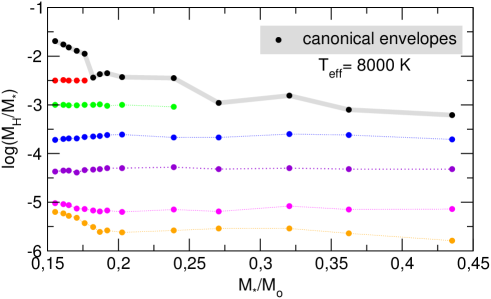
A novel aspect of this paper is the inclusion of new evolutionary sequences of low-mass He-core WDs with thin H envelopes. The consequences of the presence of thin H envelopes on the cooling ages of low-mass He-core WDs have been studied recently in Calcaferro et al. (2018). The procedure we follow to produce these new model sequences is straightforward (see the case of ZZ Ceti stars in Romero et al. 2012). For the purpose of getting a range of H envelope thicknesses, for each sequence characterized by a given value of $M_{\star}$ and a thick (canonical) value of $M_{\rm H}$, as predicted by the computation of the pre-WD evolution (second column of Table 1), we made the replacement of ¹H by ⁴He from a given mesh point, to obtain certain desired values of the H envelope mass. This artificial procedure is done at very high $T_{\rm eff}$ values at the final cooling track to wash out any unphysical transitory effects associated to this procedure long before the models reach the pulsating stage of ELMV WD stars. After changing the thickness of the H envelope, we allowed time-dependent element diffusion to act while the WD models cool down until they get to the typical values of $T_{\rm eff}$ that represent the ELMV instability strip ($T_{\rm eff}\sim 10000\$K). Diffusion strongly erodes the chemical profiles at the He/H chemical transition regions. The values of the H content that result for the different envelope thicknesses of WD models at $T_{\rm eff}\sim 8000\$K are displayed in Table 1. Also, a graphical representation of the grid of models employed in this paper is displayed in Fig. 1, where a thick (gray) line connects the canonical values of $M_{\rm H}$ as predicted by stellar evolution. Our augmented grid of models has a total of 85 sequences of low-mass He-core WD models, which contains $\sim 17000$ stellar models that were pulsationally analyzed.

Figure 2: Chemical profiles of H for WD models with $M_{\star}=0.1554M_{\sun}$, $T_{\rm eff}\sim 8000$ K and several thicknesses of H envelope (upper panel). Thick black line corresponds to the canonical envelope. Run of the logarithm of the squared Brunt–Väisälä frequency for each depicted model (lower panel). The inset shows the quantity $N/r$ as a function of the radial coordinate, $r$, for the same WD models.

Figure 3: Same as in Fig. 2, but for WD models with $M_{\star}=0.2390M_{\sun}$.

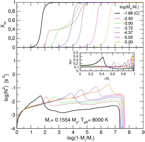
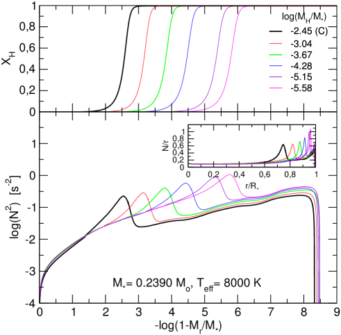
In the upper panels of Figs. 2 and 3 we show the internal chemical profiles for H corresponding to WD models at $T_{\rm eff}\sim 8000$ K with $M_{\star}=0.1554M_{\sun}$ and $M_{\star}=0.2390M_{\sun}$. In each case, we show the profile corresponding to the canonical envelope with thick black line, and the thin H envelopes with lines of different colors. For the models with $M_{\star}=0.1554M_{\sun}$ (Fig. 2), we note that the envelopes with $\log(M_{\rm H}/M_{\star})=-2.50$ and $-3.00$ have a double-layered shape, which consists of a pure H envelope surrounding a layer rich in H and He. In the other envelopes (included the canonical envelope), the transition regions are characterized by single-layered chemical profiles. Details are explained in the next Section. In the case of the models with $M_{\star}=0.2390M_{\sun}$ (Fig. 3), the He/H transition region has a single-layered shape for all the H envelope thicknesses considered.

4 Single- and double-layered chemical structure of the H envelope

Here, we show that in the case of ELM WD models, that is, WD models with stellar masses in the interval of $0.1554\leq M_{\star}/M_{\sun}\leq 0.1762$, the H envelopes can have a chemical structure of double layer, for certain interval of effective temperatures well within the instability strip of ELMV stars. We adopt the sequence with $M_{\star}=0.1554M_{\sun}$ as our test case and compute several model sequences with H envelope thicknesses in the range $-5.20\leq\log(M_{\rm H}/M_{\star})\leq-1.68$ with a small step $\Delta(M_{\rm H}/M_{\star})$. This range of envelope thicknesses includes the canonical value $M_{\rm H}=2.09\times 10^{-2}M_{\star}$ for this template sequence of models ($M_{\star}=0.1554M_{\sun}$).

Figure 4: The fractional abundance of H ($X_{\rm H}$) versus the outer mass fraction coordinate, for ELM WD models with $M_{\star}=0.1554M_{\sun}$ and $T_{\rm eff}=8000$ K. The lowest curve (thick black) corresponds to a model characterized by the thickest (canonical) envelope for this stellar mass, while the upper curves (which have been artificially displaced upwards for clarity) correspond to models with H envelopes having decreasing thicknesses. The values of $M_{\rm H}$ are shown at the right of the figure. Black (blue) curves correspond to the case of H envelopes with single-layered (double-layered) chemical structures. Black dots mark the location of each step in the chemical profile.

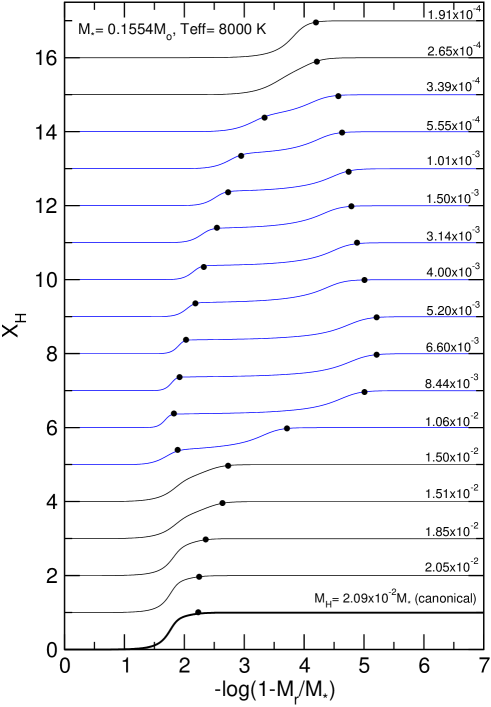
In Fig. 4 we depict the fractional abundance of H as a function of the outer mass fraction for models having $M_{\star}=0.1554M_{\sun}$ and $T_{\rm eff}\sim 8000$ K with a subset of H envelope thicknesses. The curves have been displaced upwards arbitrarily for clarity. We note that, for thick H envelopes, with values close to the canonical one ($M_{\rm H}\gtrsim 1.50\times 10^{-2}M_{\star}$), the He/H chemical transition region has a single-layered structure at $T_{\rm eff}\sim 8000$ K (lower black curves in Fig. 4). This is because such thick H envelopes experience residual H nuclear burning, and this constitutes the main energy source of the WD. This, in turn, results in very long cooling timescales (of the order of $\sim 10^{9}$ yr). Time-dependent element diffusion, acting during these long cooling timescales, strongly changes the initial shape of the H and He chemical profiles as the WD cools, forcing He to sink down and H to float to the surface.

When we consider slightly thinner H envelopes, nuclear burning is much less important in relation to the cooling timescale of the WD model, and the star cools much faster. This being the case, the diffusion timescale at the basis of the H envelope is longer than the cooling timescale of the WD. As a result, during the cooling of the star, H floats to the surface at the outer layers, but the basis of the H envelope remains virtually unaltered. The consequence of this is that the envelope has a chemical structure of double layer, consisting of a pure H envelope surrounding a H- and He-rich shell.

The presence of a double-layered chemical structure in the envelope of our models is a consequence of stellar evolution. A similar finding has been reported in detail for models of DB WD stars (e.g. Althaus & Córsico 2004). Fig. 4 shows that ELM WD models with $M_{\star}=0.1554M_{\sun}$ and $T_{\rm eff}\sim 8000$ K are expected to have a double-layered chemical structure for H envelopes with thicknesses in the range $3.4\times 10^{-4}\lesssim M_{\rm H}/M_{\star}\lesssim 1\times 10^{-2}$ (blue curves in the Figure). However, we realize that the existence of such double layers barely impacts the pulsational properties of our ELM WDs.

Finally, for H envelopes even thinner ($M_{\rm H}\lesssim 3.4\times 10^{-4}M_{\star}$), the H profile of models at the same $T_{\rm eff}$ adopts a single-layered chemical structure (upper black curves in Fig. 4). This is simply because for ELMs with very thin H envelopes, the diffusion timescale at the tail of the H distribution is extremely short (because of lower densities), much shorter than the cooling times. Hence, the star evolves into a structure with a single-layered chemical profile in a rather short period of time.

In closing, it is worth mentioning that the effect described above for the sequence of $M_{\star}=0.1554M_{\sun}$ is also verified for more massive ELM WD model sequences ($0.1554\leq M_{\star}/M_{\sun}\leq 0.1762$).

5 The impact of thin H envelopes on the pulsation properties

Figure 5: Left panels: the forward period spacing, $\Delta\Pi_{k}$ as a function of the pulsation periods, $\Pi_{k}$, for WD models with $M_{\star}=0.1554M_{\sun}$, $T_{\rm eff}\sim 8000$ K and different thicknesses of the H envelope (see Table 1 and Fig. 2). The upper panel corresponds to the WD model with canonical envelope. The thin horizontal dashed lines correspond to the value of the asymptotic period spacing, $\Delta\Pi^{\rm a}$. Right panels: the oscillation kinetic energy versus the periods for the same WD models shown in the left panel.

The shape of the chemical profiles leaves notorious signatures in the run of the squared critical frequencies, particularly, in the Brunt-Väisälä frequency ($N$). In the lower panels of Figs. 2 and 3 we show the logarithm of the squared Brunt–Väisälä frequency for models with $M_{\star}=0.1554M_{\sun}$ and $M_{\star}=0.2390M_{\sun}$ ($T_{\rm eff}\sim 8000$ K). There is a clear conection between the chemical transition regions (upper panels) and the resulting features in the run of the Brunt–Väisälä frequency for each model.

Let us now briefly examine the impact of the consideration of thin H envelopes on the mode-trapping properties of low-mass He-core WD models. Mode trapping of $g$ modes in WDs is a well-known mechanical resonance for the mode propagation, that acts due to the presence of chemical composition gradients (see Brassard et al. 1992a, b; Bradley et al. 1993; Córsico et al. 2002, for details). Observationally, a possible indication of mode trapping in a WD star is the departure from uniform period spacing. According to the asymptotic theory of stellar pulsations, in absence of chemical gradients the pulsation periods of $g$ modes with high radial order $k$ (long periods) are expected to be uniformly spaced with a constant period separation given by (Tassoul et al. 1990):

$$\Delta\Pi_{\ell}^{\rm a}=\Pi_{0}/\sqrt{\ell(\ell+1)},$$ (1)

where

$$\Pi_{0}=2\pi^{2}\left[\int_{r_{1}}^{r_{2}}\frac{N}{r}dr\right]^{-1}.$$ (2)

Actually, the period separation in chemically stratified WD model stars is not constant in anyway, except for very-high radial order modes. We define the forward period spacing as $\Delta\Pi_{k}=\Pi_{k+1}-\Pi_{k}$. Stellar models harboring a single chemical transition region (He/H) —like those considered here— local minima in $\Delta\Pi_{k}$ are generally associated with modes trapped in the H envelope, while local maxima in $\Delta\Pi_{k}$ correspond to modes trapped in the core region.

Figure 6: Same as in Fig. 5, but for WD models with $M_{\star}=0.2390M_{\sun}$ (see Table 1 and Fig. 3).

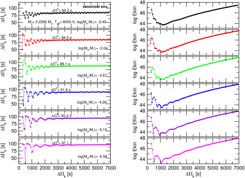
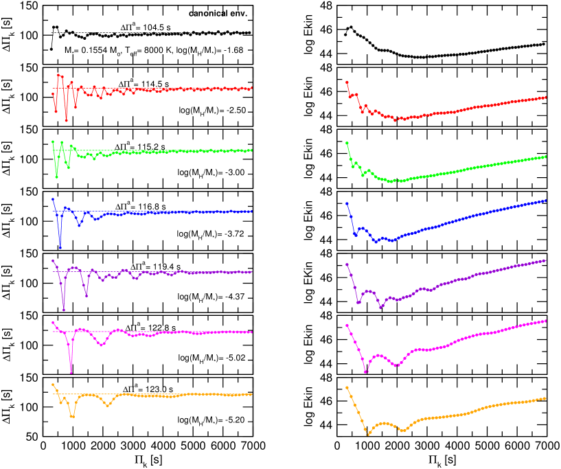
The left panels of Figs. 5 and 6 show $\Pi_{k}-\Delta\Pi_{k}$ diagrams for the same WD models depicted in Figs. 3 and 5. These models are characterized by $M_{\star}=0.1554M_{\sun}$ and $M_{\star}=0.2390M_{\sun}$ at $T_{\rm eff}\sim 8000$ K, and different thicknesses of the H envelope. In each panel, the horizontal dashed lines correspond to the asymptotic period spacing. Models with decreasing H envelope thicknesses are displayed from top to bottom, starting with the case of the canonical envelope. By examining the plots, several aspects are worth mentioning. To begin with, the asymptotic period spacing increases for decreasing H envelope thickness. This is because the integral in Eq. (2) for the quantity $\Pi_{0}$ is smaller for thinner H envelopes, by virtue that the bump in the Brunt-Väisälä frequency due to the He/H chemical interface becomes progressively narrow in the radial coordinate $r$ as this interface is located at more external layers. This can be clearly appreciated in the insets of the lower panels of Figs. 2 and 3, in which we plot the quantity $N/r$ in terms of $r$. Since $\Pi_{0}$ is larger for thinner H envelopes, the asymptotic period spacing increases (Eq. 1). In the case of the $0.1554M_{\sun}$ models, we found that $\Delta\Pi_{\ell}^{\rm a}$ experiences an increase of $15-18\%$ when we go from the canonical envelope ($\log(M_{\rm H}/M_{\star})=-1.68$) to the thinest envelope ($\log(M_{\rm H}/M_{\star})=-5.20$) for this sequence. For models with $M_{\star}=0.2390M_{\sun}$, the variation (increase) of $\Delta\Pi_{\ell}^{\rm a}$ amounts to $13-15\%$ from the canonical envelope ($\log(M_{\rm H}/M_{\star})=-2.45$) to the thinest one ($\log(M_{\rm H}/M_{\star})=-5.58$) for this sequence.

Another outstanding feature to be noted from the left panels of Figs. 5 and 6 is connected with the changes in the mode-trapping properties when we consider H envelopes progressively thinner. Indeed, we note that for thick envelopes, including the canonical one, the period-spacing distribution of $g$ modes exhibits a regular pattern of mode trapping with a very short trapping cycle —the $k$ interval ($\Delta k$) between two trapped modes. For instance, in the case of the $0.1554M_{\sun}$ models, we found a trapping cycle of $\Delta k\sim 1-3$ for H envelope thicknesses in the range $-3\lesssim\log(M_{\rm H}/M_{\star})\lesssim-1.7$. When we consider thinner H envelopes, the trapping cycle and the trapping amplitude increase. For instance, for $\log(M_{\rm H}/M_{\star})=-4.37$ we obtain $\Delta k\sim 5$, and for $\log(M_{\rm H}/M_{\star})=-5.20$ we have $\Delta k\sim 9$. A similar situation is found for the models with $M_{\star}=0.2390M_{\sun}$ (Fig. 6).

A common feature for all the values of $\log(M_{\rm H}/M_{\star})$ considered in both the $0.1554M_{\sun}$ and $0.2390M_{\sun}$ sequences is that the mode-trapping signatures reflected by $\Delta\Pi_{k}$ vanish for very large radial orders (very long periods), in which case $\Delta\Pi_{k}$ approaches to $\Delta\Pi_{\ell}^{\rm a}$, as predicted by the asymptotic theory (see Figs. 5 and 6).

Mode-trapping effects also translate into local minima and maxima in the kinetic energy of oscillation, $E_{\rm kin}$, which generally correspond to modes partially confined to the core regions and modes partially trapped in the envelope. This can be appreciated in the right panels of Figs. 5 and 6. The behaviour described above for $\Delta\Pi_{k}$ is also found in the case of $E_{\rm kin}$, that is, the mode-trapping cycle and amplitude increase with decreasing H envelope thickness. Unfortunately, the kinetic oscillation energy is a quantity very difficult to estimate from observations alone.

6 Asteroseismological analysis: period-to-period fits

Table 2: Stellar parameters derived using 1D and 3D model atmospheres of the ELMVs shown in this work.

Star	$T^{1D}_{\rm eff}$	$\log(g)^{1D}$	$M^{(1D)}_{\star}$	$T^{3D}_{\rm eff}$	$\log(g)^{3D}$	$M^{(3D)}_{\star}$
	[K]	[cgs]	[$M_{\sun}$]	[K]	[cgs]	[$M_{\sun}$]
J1112	$9590\pm 140$	$6.36\pm 0.06$	0.179a	$9240\pm 140$	$6.17\pm 0.06$	0.169b
J1518	$9900\pm 140$	$6.80\pm 0.05$	0.220a	$9650\pm 140$	$6.68\pm 0.05$	0.197b
J1738	$9130\pm 140$	$6.55\pm 0.06$	0.181c	$8910\pm 150$	$6.30\pm 0.10$	0.172b
J1735	—	—	—	$7940\pm 130$	$5.76\pm 0.08$	0.142d

Notes: ^aHermes et al. (2013b). ^b Determined using the corrections for 3D effects by Tremblay et al. (2015). ^cKilic et al. (2015). ^dBell et al. (2017).

We perform asteroseismological period-to-period fits to the complete set of ELMV stars known up to date (both confirmed and suspected). However, at variance with Calcaferro et al. (2017b), in this paper we only show the results for four out of nine ELMVs, following the suggestion of our referee. The reason is that the remainder five stars show very few periods ($\leq 3$) and/or large uncertainty in one or more of them. The spectroscopic parameters for the ELMVs shown in this work, for the 1D and 3D model atmosphere along with their uncertainties, is displayed in Table 2. As in Calcaferro et al. (2017b), we search for a model that best matches the individual pulsation periods of the star under analysis. The quality of the match between the theoretical pulsation periods ($\Pi_{k}^{\rm T}$) and the observed individual periods ($\Pi_{i}^{\rm O}$) is assessed by computing a merit function, which is defined as:

$$\chi^{2}(M_{\star},T_{\rm eff},M_{\rm H})=\frac{1}{n}\sum_{i=1}^{n}\min[(\Pi_{i}^{\rm O}-\Pi_{k}^{\rm T})^{2}],$$ (3)

where $n$ is the number of observed periods. The ELM model having the lowest value of $\chi^{2}$, if exists, is adopted as the “best-fit model”. We compute the merit function $\chi^{2}=\chi^{2}(M_{\star},T_{\rm eff},M_{\rm H})$ for our set of stellar masses ($0.1554$, $0.1612$, $0.1650$, $0.1706$, $0.1762$, $0.1805$, $0.1863$, $0.1921$, $0.2025$, $0.2390$, $0.2707$, $0.3205$, $0.3624$, and $0.4352\ M_{\sun}$), covering a wide range in effective temperature $13000\gtrsim T_{\rm eff}\gtrsim 6000\$ K and also considering the thickness of the H envelope in the interval $-5.8\lesssim\log(M_{\rm H}/M_{\star})\lesssim-1.7$ (depending on the stellar mass). This complete set comprises a total of $\sim 17000$ WD configurations.

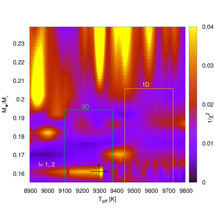
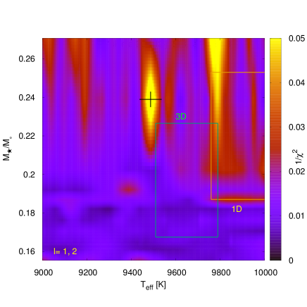
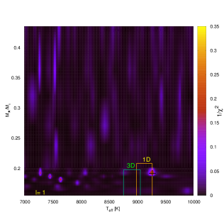
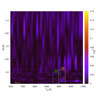
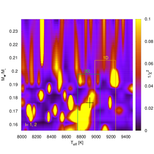
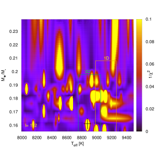
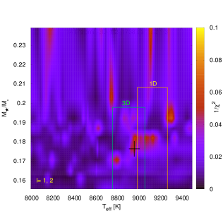
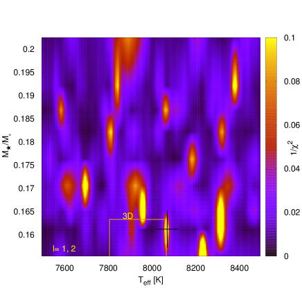
First, we consider that all of the observed periods are associated with $\ell=1$ $g$ modes, and we take the set of observed periods, $\Pi_{i}^{\rm O}$, of each star into account in order to assess the quality function given by Eq. (3). Next, we consider a mix of $g$ modes associated with both $\ell=1$ and $\ell=2$. Because we generally do not find suitable solutions for $\ell=1$ only, we display the cases for $\ell=1$ and $\ell=2$ combined with only two exceptions. Figures 7 to 11 show the projection on the effective temperature versus the stellar mass plane of the inverse of the quality function, $(\chi^{2})^{-1}$, for each ELMV under consideration, taking the corresponding set of observed periods into account, analogously to Calcaferro et al. (2017b). We include the effective temperatures and the stellar masses of every ELMV along with their uncertainties for the 1D (orange box) and 3D (Tremblay et al. 2015, green box) model atmosphere determinations. The uncertainty considered for all the stellar masses is a $15\%$ of the total mass. This is the characteristic difference in the value of the mass as derived from independent sets of evolutionary tracks (see Calcaferro et al. 2017b). Each point ($M_{\star}$,$T_{\rm eff}$) in the maps corresponds to an H envelope mass value ($M_{\rm H}/M_{\star}$) that maximizes the value of $(\chi^{2})^{-1}$ for that stellar mass and effective temperature. All ranges (for the cases with $\ell=1,2$) have been adjusted so we can show the best period fits in a region close to that of interest. As already established, the value of $\chi^{2}$ indicates the goodness of the match between the observed and the theoretical periods: the better the period match, the lower the value of $\chi^{2}$ —in the figures, the greater the value of $(\chi^{2})^{-1}$, which is shown by a color coding. If there is a single maximum for a given star, we adopt the corresponding model as the asteroseismological solution. Unfortunately, in the cases we study there are multiple possible solutions, and then we are forced to apply an external constraint to adopt one —usually, the uncertainty in the effective temperature, given by the spectroscopy and, at variance with Calcaferro et al. (2017b), we also employ the constraint of the stellar mass as given by the spectroscopic determinations.

6.1 The case of SDSS J111215.82+111745.0

SDSS J111215.82+111745.0 (hereafter J1112) exhibits a set of seven independent periods, according to Hermes et al. (2013b). At variance with Calcaferro et al. (2017b), this time we only consider the set of the five largest periods (see Table 3) because the reality of the two shortest periods ($107.56$ and $134.275\$s) has to be confirmed. The $\ell=1$ case has multiple possible solutions and we can mention that there is one fit that lies within the 1D box at $\sim 9670\$K, for $0.1869\ M_{\sun}$ and $\log(M_{\rm H}/M_{\star})=-5.19$, with $(\chi^{2})^{-1}=0.014$. The case of $\ell=1,2$ shows the best period fit at a $T_{\rm eff}$ much lower than expected ($\sim 8660\$K, for $0.1650\ M_{\sun}$ and $\log(M_{\rm H}/M_{\star})=-1.82$ (canonical), with $(\chi^{2})^{-1}=0.38$). However, if we focus on ranges closer to the values allowed by the spectroscopy, as we show in Fig. 7, we find two possible solutions, one at $\sim 9301\$K, for $0.1612\ M_{\sun}$ and $\log(M_{\rm H}/M_{\star})=-1.76$ (canonical) with $(\chi^{2})^{-1}=0.05$, and another one at $\sim 9406\$K, for $0.1706\ M_{\sun}$ and $\log(M_{\rm H}/M_{\star})=-2.48$, with $(\chi^{2})^{-1}=0.037$. We may choose the former although we note that these are not associated with very good period fits because they have low values of $(\chi^{2})^{-1}$ in comparison with the best solution.

For the purpose of establishing the accordance between the observed and theoretical periods, we assess the absolute period differences defined as $|\delta\Pi|=|\Pi^{\rm O}-\Pi^{\rm T}|$. We display in Table 3 the corresponding results for J1112 for $\ell=1,2$, where we indicate (column 6) the value of the linear nonadiabatic growth rate, $\eta$ ($\eta\equiv-\Im(\sigma)/\Re(\sigma)$, being $\Re(\sigma)$ and $\Im(\sigma)$ the real and the imaginary part, respectively, of the complex eigenfrequency $\sigma$ computed with the nonadiabatic version of the LP-PUL pulsation code (Córsico et al. 2006; Córsico & Althaus 2016)). If $\eta$ is positive (negative), the mode is unstable (stable). Unfortunately, in this case the nonadiabatic analysis predicts that these periods are stable.

Figure 7: Projection on the effective temperature versus the stellar mass plane of the inverse of the quality function considering $\ell=1,2$ for the set of periods of J1112. The value of the thickness of the H envelope for each stellar mass corresponds to the sequence with the largest value of the inverse of the quality function for that stellar mass. The boxes depict the spectroscopic $T_{\rm eff}$ and $M_{\star}$ determined for J1112 along with their uncertainties, for the 1D and 3D model atmosphere. The ranges taken in the three axes are focused on those of interest. The black cross marks the selected model.

6.2 The case of SDSS J151826.68+065813.2

SDSS J151826.68+065813.2 (hereafter J1518) exhibits seven periods (see Table 3), according to Hermes et al. (2013b). When we consider that these periods are associated with $\ell=1$, we find a possible solution at $\sim 9916\$K, for $0.1762\ M_{\sun}$ and $\log(M_{\rm H}/M_{\star})=-2.5$, with $(\chi^{2})^{-1}=0.007$, close to the 1D box. For the $\ell=1,2$ case, we find the best period fit at a value of $M_{\star}$ higher than expected ($0.4352\ M_{\sun}$, at $\sim 9717\$K, $\log(M_{\rm H}/M_{\star})=-3.69$, with $(\chi^{2})^{-1}=0.13$). If we look closer to the ranges allowed by spectroscopy as displayed in Fig. 8, we do not find any solutions within the boxes but there is a good period fit lying close, at $\sim 9487\$K, characterized by $0.2390\ M_{\sun}$, $\log(M_{\rm H}/M_{\star})=-3.67$ and $(\chi^{2})^{-1}=0.07$. It represents the best period fit in the ranges shown and we may adopt it as a solution. As in the previous case, we display in Table 3 the difference between the observed and the theoretical periods for the model we adopt.

Figure 8: Same as Fig. 7 but for J1518.

6.3 The case of PSR J1738+0333

PSR J1738+0333 is a millisecond pulsar with an ELMV as companion which we call (for short) J1738. Kilic et al. (2018) made a reanalysis of this star, where they included additional observations to the first one presented in Kilic et al. (2015). They also performed an asteroseismic analysis, and they found a range of possible solutions. We here show that study with more detail and we also perform an additional search for a period fit. Considering the different set of periods, corresponding to two years of observation, we have a set of three periods from the 2014 data set ($\Pi_{i}^{\rm O}=1788.6$, $2633.4$ and $3154.2\$s) and another set of three periods from the 2017 data set ($\Pi_{i}^{\rm O}=1833.9$, $3321.7$ and $4980.6\$s), both according to Kilic et al. (2018). We have performed three different period fits, two considering the 2014 and the 2017 data set separately, (employing the sets from Kilic et al. (2018)), and another one considering the six periods combined. This last analysis is feasible, because for pulsation measurements of different epochs of observation there is a meaningful difference in both the periods and their amplitudes, that can be associated with different modes becoming visible, as already established for ZZ Ceti stars, for instance, in Kleinman et al. (1998).

When we consider the first case (2014) for $\ell=1$, the best period fit lies at $9273\$K, with $0.1921\ M_{\sun}$, $\log(M_{\rm H}/M_{\star})=-3.02$ and $(\chi^{2})^{-1}=0.31$, that is, almost within the 1D spectroscopic box and it represents a very good solution. We show this in Fig. 9(a). For $\ell=1,2$, the best one lies at $9689\$K, with $0.4352\ M_{\sun}$, $\log(M_{\rm H}/M_{\star})=-3.21$ (canonical) and $(\chi^{2})^{-1}=13$, but it has a stellar mass larger than expected. However, as shown in Fig. 10(a), there are many other solutions, for instance within the 3D box, there is a possible solution at $8922\$K, for $0.1762\ M_{\sun}$, $\log(M_{\rm H}/M_{\star})=-5.42$ with $(\chi^{2})^{-1}=0.72$.

When we consider the second case (2017) for $\ell=1$, we find the best period fit at $9204\$K, for $0.1762\ M_{\sun}$ and $\log(M_{\rm H}/M_{\star})=-5.43$, with $(\chi^{2})^{-1}=0.16$, that is, within the 1D spectroscopic box. We show this case in Fig. 9(b). For $\ell=1,2$, the best one lies at $8554\$K, for $0.1762\ M_{\sun}$, $\log(M_{\rm H}/M_{\star})=-1.95$ (canonical), with $(\chi^{2})^{-1}=1.31$, but it has a low value of $T_{\rm eff}$. We narrow down the ranges and we show it in Fig. 10(b). Once again, there are many possible solutions. For instance, there is one at $8883\$K, for $0.1612\ M_{\sun}$ and $\log(M_{\rm H}/M_{\star})=-1.76$ (canonical), with $(\chi^{2})^{-1}=1.22$, which is a very good fit lying within the 3D box.

When we consider the 2014+2017 data combined, we find for $\ell=1$ a possible solution at $8863\$K, for $0.1921\ M_{\sun}$, $\log(M_{\rm H}/M_{\star})=-2.35$ (canonical), with $(\chi^{2})^{-1}=0.006$ (not shown). For $\ell=1,2$, we find the best solution at $9891\$K, for $0.4352\ M_{\sun}$ and $\log(M_{\rm H}/M_{\star})=-3.70$, with $(\chi^{2})^{-1}=0.18$. Focusing on more appropriate ranges, as shown in Fig. 10(c), we see that there is a good period fit lying close to the 1D box, at $9311\$K, with $0.1921\ M_{\sun}$, $\log(M_{\rm H}/M_{\star})=-3.02$, with $(\chi^{2})^{-1}=0.068$. Within the spectroscopic boxes, we find a possible solution lying at $8962\$K, for $0.1762M_{\sun}$, $\log(M_{\rm H}/M_{\star})=-1.95$ (canonical), with $(\chi^{2})^{-1}=0.062$.

From these results we can only conclude that the solutions have a stellar mass in the interval of $M_{\star}=0.1612-0.1921\ M_{\sun}$, with a constrained $T_{\rm eff}$ in the range of $\sim 8883-9273\$K, and an H envelope very poorly constrained in the range of $M_{\rm H}/M_{\star}=3.75\times 10^{-6}-1.74\times 10^{-2}$. As expected, comparing Figs. 10(a) and 10(b) with 10(c), we obtain less possible solutions when increasing the number of considered periods. Despite of this, the results obtained are not more conclusive (the solutions do not have larger values of $(\chi^{2})^{-1}$).

(a) Set of 2014, 3 periods

(b) Set of 2017, 3 periods

Figure 9: Same as Fig. 7 but for J1738, considering the periods of the 2014 data set, assuming they are associated with $\ell=1$.

(a) Set of 2014, 3 periods

(b) Set of 2017, 3 periods

(c) Set of 2014+2017, 6 periods

Figure 10: Same as Fig. 7 but for J1738, for the set of periods corresponding to 2014, 2017 and 2014+2017.

6.4 The case of SDSS J1735+2134

SDSS J1735+2134 (hereafter J1735) shows four independent periods (see Table 3), according to Bell et al. (2017). The case of $\ell=1$ shows a poor solution within the box at $8082\$K, for $0.1612\ M_{\sun}$, and $\log(M_{\rm H}/M_{\star})=-1.76$ (canonical) with $(\chi^{2})^{-1}=0.007$, while for the case of $\ell=1,2$, the period fit with the best value is associated with a model consisting of $0.2390\ M_{\sun}$ (at $9892\$K and $\log(M_{\rm H}/M_{\star})=-4.28$, with $(\chi^{2})^{-1}=0.53$), once again, outside the allowed ranges. If we focus in the ranges allowed by spectroscopy as in Fig. 11, we can see good period fits close to the box at $7963\$K, for $0.1650\ M_{\sun}$ and $\log(M_{\rm H}/M_{\star})=-1.82$ (canonical), with $(\chi^{2})^{-1}=0.23$ and another at $8075\$K, for $0.1612\ M_{\sun}$ and $\log(M_{\rm H}/M_{\star})=-1.76$ (canonical), with $(\chi^{2})^{-1}=0.22$. This last period fit may be choosen as a solution, and it is the same result obtained in Calcaferro et al. (2017b). We display the comparison between theoretical and observed periods in Table 3.

Figure 11: Same as Fig. 7 but for J1735.

Table 3: Observed and theoretical periods ($\ell=1,2$) for the asteroseismological models for J1112 with ($M_{\star}$,$T_{\rm eff}$,$\log(M_{\rm H}/M_{\star})$) = ($0.1612\ M_{\sun}$, $9301\$ K, $-1.76$), for J1518 with ($0.2390\ M_{\sun}$, $9487$ K, $-3.67$) and for J1735 with ($0.1612\ M_{\sun}$, $8075\$K, $-1.76$). The harmonic degree $\ell$, the radial order $k$, the absolute period difference, and the nonadiabatic growth rate for each theoretical period are also displayed.

Star	$\Pi^{\rm O}$[s]	$\Pi^{\rm T}$[s]	$\ell$	$k$	$|\delta\Pi|$[s]	$\eta[10^{-4}]$	Remark
J1112	$1792.905\pm 0.005$	$1797.822$	$1$	$17$	$4.92$	$-0.00004$	stable
	$1884.599\pm 0.004$	$1886.039$	$2$	$32$	$1.44$	$-0.0155$	stable
	$2258.528\pm 0.003$	$2266.323$	$2$	$39$	$7.79$	$-0.131$	stable
	$2539.695\pm 0.005$	$2536.215$	$2$	$44$	$3.48$	$-0.399$	stable
	$2855.728\pm 0.01$	$2861.968$	$2$	$50$	$6.24$	$-1.14$	stable
J1518	$1335.318\pm 0.003$	$1329.599$	$2$	$28$	$5.719$	$0.463$	unstable
	$1956.361\pm 0.003$	$1959.913$	$1$	$24$	$3.552$	$0.653$	unstable
	$2134.027\pm 0.004$	$2131.306$	$2$	$46$	$2.721$	$0.504$	unstable
	$2268.203\pm 0.004$	$2266.188$	$1$	$28$	$2.015$	$0.766$	unstable
	$2714.306\pm 0.003$	$2717.686$	$2$	$59$	$3.380$	$-0.373$	stable
	$2799.087\pm 0.005$	$2802.873$	$1$	$35$	$3.786$	$1.14$	unstable
	$3848.201\pm 0.009$	$3851.967$	$2$	$84$	$3.766$	$-4.96$	stable
J1735	$3362.76\pm 0.54$	$3359.87$	$2$	$56$	$2.89$	$5.57$	unstable
	$3834.54\pm 0.42$	$3831.65$	$2$	$64$	$2.89$	$0.243$	unstable
	$4541.88\pm 0.24$	$4542.92$	$2$	$76$	$1.04$	$-14.3$	stable
	$4961.22\pm 0.72$	$4960.70$	$1$	$48$	$0.52$	$13.9$	unstable

7 Summary and conclusions

In this work, we have presented a thorough asteroseismological analysis of pulsating ELM WD stars on the basis of our complete set of fully evolutionary models that represent low-mass He-core WDs harboring a range of H envelope thicknesses. This is the sixth paper in a series of works dedicated to the study of pulsating low-mass He-core WDs (including ELMVs). Here, we first explored the chemical profiles of the grid of models having different H envelope thicknesses, and also the impact on the adiabatic pulsation properties. Furthermore, we performed an asteroseismological analysis to four ELMV stars, those that show a sufficiently high number of periods and with small uncertainties to allow us to draw robust asteroseismological conclusions, in analogy to that of Calcaferro et al. (2017b), but this time employing this larger set of evolutionary sequences that expands the parameter space by incorporating the thickness of the H envelope as a free parameter.

Next, we present a brief summary of the main results of this work:

• The analysis of the internal chemical profiles of our ELM WDs models with thin H envelope puts in evidence the existence of a double-layered shape of the H envelope for some models lying well within the instability strip.

• When we considered thin H envelopes and analyzed the impact on the mode trapping properties of $g$ modes of our ELM WDs, we found that they strongly depend on $M_{\rm H}$. The period-spacing distribution acquires a steady form for thick envelopes (including the canonical one), with a very short trapping cycle, while for thinner H envelopes both the trapping cycle and the trapping amplitude increase.

• The asymptotic period spacing increases for decreasing H envelope thickness.

• The period-to-period fits show multiple solutions. Only with the inclusion of external constraints (i.e., spectroscopy values) we were able to adopt a model and in one case, we could only give a range of possible solutions. The results are condensed in Table 4.

• Some of the solutions found (see Table 4) are characterized by thick (canonical) H envelopes and some by thin H envelopes. This result reinforces the findings of Calcaferro et al. (2018) about the possible existence of ELM WDs with thin H envelope, thus leading to the possibility that they could have been formed through unstable mass loss, for instance, via common-envelope episodes.

• Most of the solutions we adopted have a lower value of the stellar mass than those adopted in Calcaferro et al. (2017b). The reason for this may be related to the fact that we are employing models with thinner H envelope and also because we are using a new constraint, the stellar mass.

• We generally did not find appropriate solutions considering modes associated only with $\ell=1$, but with a mixture of $\ell=1,2$. Moreover, in most cases we found that the pulsation periods corresponding to the adopted asteroseismological models are associated with pulsationally unstable modes.

Given the scarcity of observed periods in the ELM WDs it is very difficult to apply the methods of asteroseismology, specifically, to find a unique solution compatible with the spectroscopic determinations. This forces us to focus our exploration on the range of parameters (observational boxes) dictated by the spectroscopy. In addition, when there is a change in the periods determined for one star, the solutions change considerably. Furthermore, only for one case, J1112, our non-adiabatic computations predict that the adopted solutions are not pulsationally unstable.

For the purpose of comparison with our previous work, in Table 5 we show the asteroseismological results obtained in the present paper and in Calcaferro et al. (2017b). J1735 has not been included in the Table because we obtain the exact same solution when we allow the H-envelope thickness to vary. It is interesting to note that, when we incorporate the thickness of the H envelope as a free parameter, for J1112 we still obtain a solution with a canonical H envelope, although it is a different one because now we use the constraint of the stellar mass to adopt a solution. On the whole, we can conclude that the asteroseismological models in general change when the H-envelope thickness is taken as a variable.

All in all, in this paper we have presented a thorough asteroseismological study of ELMVs, using a complete set of fully evolutionary models of He-core ELM WDs with different H envelope thicknesess. In this way, we have pushed the limits of what is possible in terms of deriving the internal structure of these stars through asteroseismological period fits based on this grid. In order to achieve progress in this field, and obtain more robust asteroseismological solutions, it is necessary to obtain richer observations of the pulsations of these stars. Indeed, due to the few periods detected, we had to restrict ourselves to show the results for stars with the richest period spectra and the less uncertainty in their periods. The detection of a larger number of pulsation periods of the known ELMVs, and the discovery of new ELMV stars, will allow a substantial progress in the knowledge of the internal structure of low mass WD stars, the nature of their predecessors, and the evolutionary channels that lead to their origin (see Calcaferro et al. 2018).

Table 4: Main characteristics of the adopted asteroseismological models and of the ranges of possible solutions for the ELMVs shown in this work.

Star	$T_{\rm eff}$ [K]	$\log(g)$ [cgs]	$M_{\star}[M_{\sun}]$	$\log(M_{\rm H}/M_{\star})$	$\log(R_{\star}/R_{\sun})$	$\log(L_{\star}/L_{\sun})$
J1112∗	9301	5.9695	0.1612	-1.76	-1.1623	-1.4932
J1518	9487	6.9994	0.2390	-3.67	-1.5916	-2.3200
J1738	[8883,9273]	[6.0506,6.6923]	[0.1612,0.1921]	[-5.43,-1.76]	[-1.5057,-1.2029]	[-2.2548,-1.6560]
J1735∗	8075	6.2241	0.1612	-1.76	-1.2899	-1.9957

Note: ^∗ Solution with canonical H envelope.

Table 5: Comparison between the main characteristics of the adopted asteroseismological models for every ELMV WD shown in this work with the results obtained in Calcaferro et al. (2017b).

Star	Work	$T_{\rm eff}$ [K]	$\log(g)$ [cgs]	$M_{\star}[M_{\sun}]$	$\log(M_{\rm H}/M_{\star})$	$\log(R_{\star}/R_{\sun})$	$\log(L_{\star}/L_{\sun})$
J1112	This	9301	5.9695	0.1612	-1.76	-1.1623	-1.4932
	Previous	9300	6.9215	0.2390	-2.45	-1.5528	-2.2757
J1518	This	9487	6.9994	0.2390	-3.67	-1.5916	-2.3200
	Previous	9789	7.0956	0.2707	-2.96	-1.6126	-2.3098
J1738	This	[8883,9273]	[6.0506,6.6923]	[0.1612,0.1921]	[-5.43,-1.76]	[-1.5057,-1.2029]	[-2.2548,-1.6560]
	Previous	9177	7.6241	0.4352	-3.21	-1.7746	-2.7447