On the Nature of the X-ray Emission from the Ultraluminous X-ray Source, M33 X-8: New Constraints from NuSTAR and XMM-Newton

Abstract

We present nearly simultaneous NuSTAR and XMM-Newton observations of the nearby (832 kpc) ultraluminous X-ray source (ULX) M33 X-8. M33 X-8 has a 0.3–10 keV luminosity of $L_{\_}{\rm X}\approx 1.4\times 10^{39}$ erg s^-1, near the boundary of the “ultraluminous” classification, making it an important source for understanding the link between typical Galactic X-ray binaries and ULXs. Past studies have shown that the 0.3–10 keV spectrum of X-8 can be characterized using an advection-dominated accretion disk model. We find that when fitting to our NuSTAR and XMM-Newton observations, an additional high-energy ($\;\buildrel>\over{\sim}\;$10 keV) Comptonization component is required, which allows us to rule out single advection-dominated disk and classical sub-Eddington models. With our new constraints, we analyze XMM-Newton data taken over the last 17 years to show that small ($\approx$30%) variations in the 0.3–10 keV flux of M33 X-8 result in spectral changes similar to those observed for other ULXs. The two most likely phenomenological scenarios suggested by the data are degenerate in terms of constraining the nature of the accreting compact object (i.e., black hole versus neutron star). We further present a search for pulsations using our suite of data; however, no clear pulsations are detected. Future observations designed to observe M33 X-8 at different flux levels across the full 0.3–30 keV range would significantly improve our constraints on the nature of this important source.

1 Introduction

Ultraluminous X-ray sources (ULXs) are often defined as off-nuclear X-ray point sources with luminosities that exceed $L_{\_}{\rm X}\approx 10^{39}$ erg s^-1, the classical Eddington limit for a 10 $M_{\_}\odot$ black hole (BH). Over the last two decades, new observations and theoretical models suggest that most ULXs are predominantly powered by super-Eddington accretion onto neutron stars (NSs) and stellar-mass BHs (i.e., $\;\buildrel<\over{\sim}\;$10 $M_{\_}\odot$), as opposed to sub-Eddington accretion onto intermediate-mass BHs (see Kaaret et al. 2017 for a comprehensive review). Much of these insights have been gained thanks to XMM-Newton and NuSTAR observations of the brightest nearby ULXs (see, e.g., Gladstone et al. 2009; Walton et al. 2018a), and the emergence of theoretical models that have been instrumental in explaining the observed spectra.

Modulo some uncertainty on details, it is generally thought that as accretion onto the compact object approaches the Eddington limit, radiation pressure will increase the scale height of the innermost portions of the disk, leading to local mass loss in a radiatively-driven wind and inward advection of energy, as per the “slim” disk model (e.g., Abramowicz et al. 1988; Mineshige et al. 2000). The bulge of the inner disk and wind columns can form a funnel-like structure that leads to geometric beaming of radiation for vantage points that are close to the rotation axis (e.g., Poutanen et al. 2007; King 2009; Dotan & Shaviv 2011). For the case of a NS accretor, the accretion disk may be interrupted within the magnetospheric radius, where material will flow along the magnetic field lines to the NS magnetic poles (e.g., King & Lasota 2016; Mushtukov et al. 2017).

Whether NS or BH accretors dominate the ULX population as a whole is a subject of current debate. At present, there are only four extragalactic ULXs that have been discovered to contain NS accretors on the basis of pulsations: M82 X-2, NGC 7793 P13, NGC 5907 ULX1, NGC 300 ULX1, and SMC X-3 (e.g., Bachetti et al. 2014; Fürst et al. 2016; Israel et al. 2017; Carpano et al. 2018; Tsygankov et al. 2017), and also one Galactic accreting pulsar ULX: Swift J0243.6+6124 (Wilson-Hodge et al. 2018). There are also a few Galactic BH sources that reach super-Eddington accretion rates, such as GRS 1915+105 (e.g., Done et al. 2004), V4641 Sgr (Revnivtsev et al. 2002), and V404 Cyg (Jourdain et al. 2017), suggesting ULXs are very likely to be a mixed NS and BH population. However, population synthesis arguments (see, e.g., Wiktorowicz et al. 2017) and observational biases against detecting pulsations (e.g., King et al. 2017, Mushtukov et al. 2017) suggest that many more ULXs may contain NS compact objects than previously thought. Recent observational studies have shown that the hard spectral shape associated directly with the pulsed emission in pulsar ULXs can be used to successfully model the hard spectral component of non-pulsar ULXs, suggesting that many more NS ULXs may be lurking in the broader ULX population (e.g., Walton et al. 2018b, hereafter, W18; Koliopanos et al. 2017; Pintore et al. 2017).

To date, the majority of the broad band high signal-to-noise ULX spectra have come from highly super-Eddington objects, with $L_{\_}{\rm X}=$(5–100) $\times 10^{40}$ erg s^-1. In this paper, we explore the case of M33 X-8, a relatively nearby ($D=832$ kpc; Bhardwaj et al. 2016), low-luminosity ($L_{\_}{\rm 0.3-10~{}keV}\approx 10^{39}$ erg s^-1) ULX. Given its corresponding high flux ($10^{-11}$ erg cm^-2 s^-1), which is comparable to the fluxes of many of the luminous ULXs, M33 X-8 provides the best opportunity to constrain the properties of a ULX that is at the transition between luminous Galactic BH XRBs and the broader extragalactic ULX population. The source is located in the nuclear region of M33, which initially suggested that the X-8 was a possible AGN (Long et al. 1981). However, a lack of any expected luminous optical counterparts (Long et al. 2002) and tight upper limits on the central supermassive black hole mass of M33 ($\;\buildrel<\over{\sim}\;$1500 $M_{\_}\odot$; e.g., Gebhardt et al. 2001; Davis et al. 2017), indicated that the source is a ULX. Furthermore, there are a number of young ($\;\buildrel>\over{\sim}\;$50 Myr) early-type stars in the nuclear region of M33, with which the source could be associated (Long et al. 2002; Garofali et al. 2018).

A comprehensive spectral characterization of M33 X-8 was previously performed by Middleton et al. (2011; hereafter, M11) using 12 XMM-Newton observations that spanned a three-year baseline. M11 performed stacked spectral fitting for three distinct flux (luminosity) ranges and found that the 0.3–10 keV spectrum of M33 X-8 could be modeled well using both sub-Eddington (hot accretion disk plus optically-thin/hot Comptonization) and super-Eddington (slim disk and slim disk plus optically-thick/cold Comptonization) models, preventing tight constraints on the nature of the accretion onto this source.

Here, we present a first coordinated broad band (0.3–30 keV) spectrum from temporally overlapping 24 ks XMM-Newton and 102 ks NuSTAR observations, and provide spectral and timing analyses of this data set ($\S$3.1). We consider both the models provided by M11, which were presumed to include a BH accretor, and also the more recent NS-based model from W18 that provides good fits to the broad band spectra of luminous ULXs. Using knowledge of the spectral components from our XMM-Newton plus NuSTAR fits, we revisit the spectral variability of this source using observations from the XMM-Newton archive, which includes 17 XMM-Newton observations that span 17 years. To further assess the nature of the source, we perform a search for pulsations in this object. Throughout this paper, we assume a Galactic column density of $N_{\_}{\rm H}=5.7\times 10^{20}$ cm^-2 in the direction of M33 (Dickey & Lockman 1990), and include this column in all spectral fits. Unless stated otherwise, quoted uncertainties throughout this paper correspond to 90% confidence intervals.

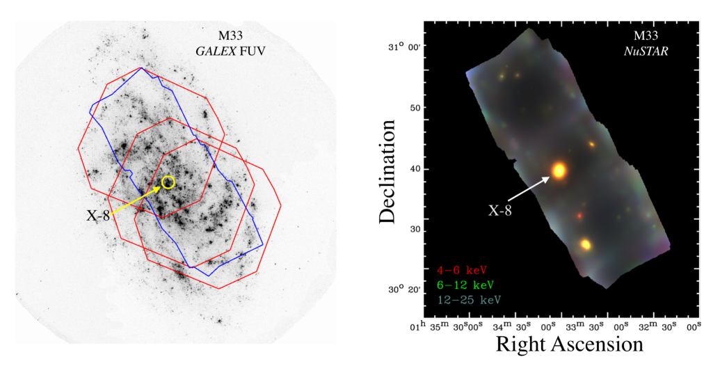
Figure 1: (Left) GALEX FUV image of M33 with the aerial footprints of the NuSTAR (blue region) and recent XMM-Newton (red regions) observations (from July–August 2017) are overlaid. The position of M33 X-8 is indicated. Our observational strategy permitted X-8 to be observed in all three XMM-Newton exposures. (Right) Three-color NuSTAR image mosaic of the M33 legacy fields. The image was constructed from 4–6 keV ($red$), 6–12 keV ($green$), and 12–25 keV ($blue$) exposure-corrected adaptively smoothed images.

Table 1: XMM-Newton Observation Log

		Useful Exposure (ks)
					Off-Axis Angle	$F_{\_}{\rm X}$ (0.3–10 keV)
Obs Date	Obs ID	PN	MOS1	MOS2	(arcmin)	($10^{-11}$ ergs s-1)	Bin	PI
(1)	(2)	(3)	(4)	(5)	(6)	(7)	(8)	(9)
2000 Aug 02	0102640401	0	13.0	12.9	13.2	1.52	2	B. Aschenbach
2000 Aug 04	0102640101a	7.5	10.6c	10.5c	0.3	1.67	3	B. Aschenbach
2000 Aug 07	0102640301a	3.7d	10.0	7.3	13.6	1.68	3	B. Aschenbach
2001 Jul 05	0102640601	3.2b,d	4.7d	4.7d	7.4	1.69	3	B. Aschenbach
2001 Jul 05	0102640701	0	11.5	11.6	13.2	1.73	4	B. Aschenbach
2001 Aug 15	0102642001a	8.8	11.5	11.5	13.3	1.81	4	B. Aschenbach
2002 Jan 25	0102642101a	10.0b	12.3	12.3	10.6	1.67	3	B. Aschenbach
2002 Jan 27	0102642301a	10.0d	12.3	12.3	7.2	1.56	2	B. Aschenbach
2003 Jan 23	0141980601a	11.5	13.5	13.6	13.2	1.85	4	W. Pietsch
2003 Jan 24	0141980401a	0	1.8	1.4	13.6	1.83	4	W. Pietsch
2003 Feb 12	0141980801a	8.1	10.2	10.2	0.3	1.46	1	W. Pietsch
2003 Jul 11	0141980101a	6.3d	7.3	8.3	11.0	1.61	3	W. Pietsch
2010 Jul 09	0650510101	69.6d	100.8	100.7b,d	7.8	1.74	…f	B. Williams
2010 Jul 11	0650510201	71.0	101.1	101.1	5.2	1.54	2	B. Williams
2017 Jul 21	0800350101	18.6	21.6	21.6	8.3	1.79	4	B. Lehmer
2017 Jul 23	0800350201e	20.9b	22.6	22.6	1.5	1.58	2	B. Lehmer
2017 Aug 02	0800350301	21.6d	23.3	23.3	10.9	1.62	3	B. Lehmer

Note—The medium optical blocking filter was used for all three EPIC cameras in each of these observations except in ObsIDs: 0102640301 (thin filter 2 used for MOS2), 0102640401 (thick filter used for all three detectors), 0650510101 and 0650510201 (thin filter 1 used for pn in both). Col.(1): Start date of the observation. All rows are order by ascending date. Col.(2): Unique XMM-Newton observation ID. Col.(3)–(5): Cumulative good-time-interval exposure times for pn, MOS1, and MOS2 after filtering for flaring (see $\S$2.2 for details). Col.(6): EPIC pn-based off-axis angle in units of arcmin. Col.(7): 0.3–10 keV flux, as measured by fitting the individual ObsID pn data to a TBABS $\times$ (DISKPBB + COMPTT) model (see $\S$3.2 for details). Col.(8): Designated flux bin value used for joint spectral fitting in $\S$3.3. Sources with $F_{\_}{\rm X}$/($10^{-11}$ erg cm^-2 s^-1) $<1.5$, 1.5–1.6, 1.6–1.7, and $>1.7$ are given bins 1, 2, 3, and 4, respectively. Col.(9): PI of the ObsID. Original works from archival observations can be found in Pietsch et al. (2004) and Williams et al. (2015).
^a MOS observations used by M11.
^b Corrected for pileup following the procedure described in $\S$2.2.
^c Exposure taken in Small Window Mode.
^d Core of X-8 PSF on or very near (within $\sim 25$″) a CCD gap or FOV edge.
^e Observation exposure overlaps NuSTAR observation (ObsID 50310002003).
^f Excluded from flux-binned spectral fitting due to high fractional variability and investigated individually in $\S$3.2.

2 Data and Spectral Extractions

M33 was observed by NuSTAR in three unique $12\times 12$ arcmin² fields over two separate epochs (i.e., six total observations) that occurred in February and March of 2017 (epoch 1; ObsID: 50310002001) and July and August of 2017 (epoch 2; ObsID: 50310002003) as a part of the M33 NuSTAR Legacy program. In addition to placing constraints on the nature of M33 X-8 (the subject of this paper), the M33 NuSTAR Legacy program was designed to help characterize accretion states for the XRB population throughout the galaxy. A forthcoming publication (Yang et al. in-prep) will address the properties of the M33 XRB population more broadly. Figure 1 shows GALEX FUV and NuSTAR three-color mosaic images of the M33 region.

The first epoch of NuSTAR observations covered X-8 in one of the three observations. Unfortunately, only one nearly simultaneous observation with the Neil Gehrels Swift Observatory was conducted during this epoch, and it did not contain X-8 in its field of view (FOV). We therefore do not make use of Swift data in this study. Furthermore, given the lack of nearly simultaneous low-energy (i.e., $<$3 keV) data, and a brief inspection showing little difference between the NuSTAR spectra between epochs 1 and 2 (the 3–30 keV spectrum of epoch 1 is consistent with a very small constant offset of $\approx$2%), we chose not to make use of the epoch 1 data when analyzing spectra. We do, however, consider the epoch 1 data when searching for pulsations; and details of this analysis are presented in $\S$3.4. The second epoch of NuSTAR observations, which constitute the focus of this study, were accompanied by nearly simultaneous XMM-Newton observations of the three fields. During epoch 2, X-8 was observed once by NuSTAR; however, thanks to the larger field of view (FOV) of XMM-Newton ($27.5\times 27.5$ arcmin² for pn and $33\times 33$ arcmin² for MOS), X-8 was covered by all three of the XMM-Newton observations (see red XMM-Newton pn FOV outlines in Fig. 1). The new observations, presented here, thus consist of three XMM-Newton exposures of M33 X-8 (each 23–25 ks), with one XMM-Newton epoch (ObsID: 0800350201) being nearly simultaneous with the 102 ks NuSTAR ObsID: 50310002003, which occurred on 2017 July 23.

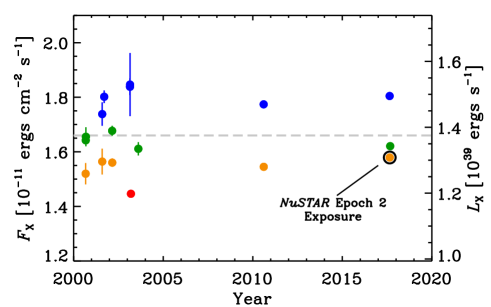
Figure 2: 0.3–10 keV flux (and luminosity) versus time for the XMM-Newton EPIC-pn archival observations. Colors represent different flux bins, as used in the spectral grouping performed in $\S$3.2, with $F_{\_}{\rm X}$/($10^{-11}$ erg cm^-2 s^-1) $<1.5$, 1.5–1.6, 1.6–1.7, and $>1.7$, displayed as red, orange, green, and blue, respectively. The observation containing the nearly simultaneous NuSTAR exposure of M33 X-8 is annotated with a black open circle. The flux of M33 X-8 over the last 17 years has remained very stable with a mean value and standard deviation of $F_{\_}{\rm X}=(1.66\pm 0.10)\times 10^{-11}$ erg cm^-2 s^-1 ($L_{\_}{\rm X}=[1.38\pm 0.09]\times 10^{39}$ erg s^-1). The X-ray flux of X-8 was near its average value during our simultaneous XMM-Newton and NuSTAR observation.

When analyzing the spectral properties of X-8, we first use the nearly simultaneous NuSTAR and XMM-Newton observations during epoch 2 to constrain the 0.3–30 keV spectrum. We use this observational set to create “baseline” spectral models of the source, which we then apply to both the new XMM-Newton data from 2017 (described previously in this section), as well as archival XMM-Newton data. In Table 1, we provide an XMM-Newton observation log for the data used in this program, and in Figure 2, we show the measured 0.3–10 keV flux of X-8 versus time for the entire XMM-Newton archival history. Several of the available XMM-Newton observations (ObsIDs 0102640801, 0102641001, 0141980301, 0141980501 and 0672190301) that contain M33 X-8 in the FOV suffered from observation issues (e.g., slew failure, high levels of background radiation, and telemetry glitches) and were therefore excluded from this study. In the subsections below, we describe our data reduction and spectral extraction procedures pertaining to X-8.

2.1 NuSTAR Reductions

The NuSTAR data was reduced using HEASoft v6.20, NuSTAR Data Analysis Software (NuSTARDAS) v1.7.1, and CALDB version 20170503. We processed level 1 data to level 2 products by running nupipeline, which performs a variety of data reduction steps, including (1) filtering out bad pixels, (2) screening for cosmic rays and observational intervals when the background was too high (e.g., during passes through the SAA), and (3) projecting accurately the events to sky coordinates by determining the optical axis position and correcting for the dynamic relative offset between the optics bench and focal-plane bench due to motions of the 10 m mast that connects the two benches. A total “cleaned” exposure of 101.5 ks in epoch 2 was utilized for this analysis.

M33 X-8 source spectra were extracted from a 40″ radius circular aperture, centered at ($\alpha$,$\delta$)${}_{\_}{\rm J2000}$ = 01^h 33^m 50.6^s, $+30^{\circ}$ 39′ 31″, the centroid of the NuSTAR point-source emission. The aperture size was chosen to both encompass a large fraction of the point-spread function (PSF) and also ensure large signal-to-noise for the highest possible energies in our spectra. We further inspected 2–8 keV images from the Chandra ACIS Survey of M33 (ChASeM33; Tüllmann et al. 2011) and found that there were no additional sources within this aperture to the deep limits in ChASeM33. We extracted background spectra from three circular apertures, located well outside the PSF of X-8, yet within the same chip as X-8, in regions without any obvious sources detectable by eye. These background regions cover a total area of 17.28 arcmin², and were chosen to be the same between FPMA and FPMB. Source and background spectra, along with redistribution matrices and auxiliary response files (RMFs and ARFs) were produced using nuproducts with the spectra grouped to a minimum of 50 counts per energy bin and analyzed across the 3–30 keV energy range, where the source counts were observed to exceed the background counts.

2.2 XMM-Newton Reductions

The reduction of XMM-Newton data was carried out with the XMM-Newton Science Analysis System (SASv16.0.0), following the procedures recommended in the online user guides. Calibrated events lists for the EPIC pn (Strüder et al. 2001) and MOS (Turner et al. 2001) detectors were produced using epchain and emchain, respectively. Good time intervals (GTIs) were established from the full field light curve between 10 keV and 12 keV for pn and at $>10$ keV for MOS; periods of relatively high count rate ($>0.4$ counts s^-1 for pn and $>0.35$ counts s^-1 for MOS) were removed from the events lists to account for background flaring. Standard filters were then applied to allow only single and double events (PATTERN$<$=4 and FLAG==0) in the pn events list and only single events (PATTERN==0 and flag = #XMMEA_EM) for MOS.

Pile-up was evaluated using the ratios of modeled-to-observed single and double patterns which are output by epatplot for a circular region of radius $45$″ around the source in all detectors. When the ratio of singles was less than 1 and doubles greater than 1, the observation was considered to be piled-up. For such observations, pile-up was corrected by extracting spectra from annuli with outer radii of 45″ and inner radii of 5″ and 10″ for MOS and pn, respectively. Pile-up corrections were implemented for the pn data in ObsIDs 0102640601, 0102642101, and 0800350201 and for MOS2 in ObsID 0650510101 following our procedure. Out-of-time (OoT) events were found to be negligible ($\;\buildrel<\over{\sim}\;$0.3%) in all observations and were therefore not removed from pn or MOS spectra.

RMFs and ARFs were generated using SAS commands rmfgen and arfgen, respectively. Source spectra were then extracted from the fully filtered events lists in circular regions with radii of $45$″(or annular regions in the case of pile-up; see above), centered on the source with the SAS command evselect. Background spectra were extracted from the same events lists, in circular regions with radii of $45$″ on the same CCD as the source but free from obvious contaminating point sources (i.e., sources visible by eye in 0.3–10 keV images). Spectra were grouped to have a minimum of 50 counts per energy bin, and analyzed across the full 0.3–10.0 keV energy range.

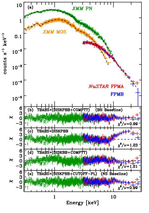
Figure 3: (a) Best-fit 0.3–30 keV spectrum of M33 X-8 for our nearly-simultaneous NuSTAR (ObsID: 50310002003) and XMM-Newton (ObsID: 0800350201) observations. The data are shown for the XMM-Newton pn (green), MOS1 and MOS2 (orange), and NuSTAR FPMA (red) and FPMB (blue) cameras. Best-fit residuals for pn and NuSTAR cameras are shown (MOS is excluded for clarity of viewing) for models ($b$) TBABS $\times$ (DISKPBB + COMPTT), which is our BH baseline model, ($c$) TBABS $\times$ DISKPBB, ($d$) TBABS $\times$ (DISKBB + COMPTT), and ($e$) our NS baseline model TBABS $\times$ (DISKPBB + CUTOFF-PL). Detailed physical descriptions of these models are provided in $\S$3.1. The M11 study of X-8 had shown that models ($b$)–($d$) provided acceptable fits to the XMM-Newton archival data; however, we find that only our baseline models are acceptable when using the combined XMM-Newton plus NuSTAR data.

Table 2: Best fit parameters for Nearly-Simultaneous NuSTAR plus XMM-Newton Observation.

				(BH Baseline)	(NS Baseline)
Parameter	Unit	DISKPBB	DISKBB + COMPTT	DISKPBB + COMPTT	DISKPBB + CUTOFF-PL
$N_{\_}{\rm H}$	1022 cm-2	$0.169\pm 0.005$	$<0.0004$	$0.133_{\_}{-0.006}^{+0.016}$	$0.142\pm 0.006$
$kT_{\_}{\rm in}$	keV	$1.73\pm 0.03$	0.751$\pm 0.018$	1.06${}_{\_}{-0.22}^{+0.29}$	$1.37\pm 0.03$
$p$		$0.523\pm 0.004$	…	$0.569_{\_}{-0.024}^{+0.009}$	$0.553_{\_}{-0.006}^{+0.007}$
$(R_{\_}{\rm in}/D_{\_}{10})^{2}\cos\theta$		$0.0267\pm 0.0027$	$1.77_{\_}{-0.11}^{+0.13}$	$0.25_{\_}{-0.15}^{+0.26}$	$0.086_{\_}{-0.010}^{+0.011}$
$kT_{\_}{\rm comp}$	keV	…	$129_{\_}{-5}^{+4}$	$16_{\_}{-13}^{+144}$	…
$\tau$		…	$<0.41$	$<9.1$	…
$\Gamma$		…	…	…	0.5⋆
$E_{\_}{\rm cut}$	keV	…	…	…	8.1⋆
Norm${}_{\_}{\rm comp}$	$10^{-5}$	…	$1.0_{\_}{-0.03}^{+6.9}$	$3.9_{\_}{-3.5}^{+11}$	$6.71\pm 0.48$
$C_{\_}{\rm MOS1}$		$0.93\pm 0.01$	$0.93\pm 0.01$	$0.93\pm 0.01$	$0.93\pm 0.01$
$C_{\_}{\rm MOS2}$		$0.95\pm 0.01$	$0.94\pm 0.01$	$0.95\pm 0.01$	$0.95\pm 0.01$
$C_{\_}{\rm FPMA}$		$1.08\pm 0.02$	$1.19\pm 0.02$	$1.12\pm 0.03$	$1.12\pm 0.03$
$C_{\_}{\rm FPMB}$		$1.07\pm 0.02$	$1.18\pm 0.02$	$1.11\pm 0.03$	$1.11\pm 0.03$
$\chi^{2}/\nu\;(\nu)$		1.23 (1714)	1.21 (1712)	0.99 (1711)	0.99 (1713)
Null $P$		$5.4\times 10^{-11}$	$6.7\times 10^{-9}$	0.62	0.56

Note—The Galactic column density $N_{\_}{\rm H,Gal}=5.7\times 10^{20}$ cm^-2 has been applied to all of the above fits. All quoted errors are at the 90% confidence level.
^⋆Indicates parameter was fixed to the listed value (see $\S$3.1 for details).

3 Analysis and Results

3.1 Simultaneous NuSTAR plus XMM-Newton Spectral Fitting

We began by fitting our nearly simultaneous NuSTAR and XMM-Newton observations using XSPEC v. 12.9.1 (Arnaud 1996). All fits were performed using the XMM-Newton pn, MOS1, and MOS2, and NuSTAR FPMA and FPMB data as described in $\S$2. To account for cross-calibration uncertainties and potential small flux variations (NuSTAR and XMM-Newton data were not taken exactly simultaneously), we made use of a free CONSTANT model, which we chose to be fixed at a value of 1.0 for the XMM-Newton pn data. Source and background counts were binned as described in $\S$2, and source spectra were fit by minimizing the $\chi^{2}$ statistic, after background counts were subtracted. For all XMM-Newton data, the background is estimated to be a factor of $>$10 times lower than the source. For NuSTAR, the background remains a factor of 5 times lower that the source for $E<20$ keV, and is comparable to the source level at $E=$ 20–30 keV, where background emission lines are known to be present.

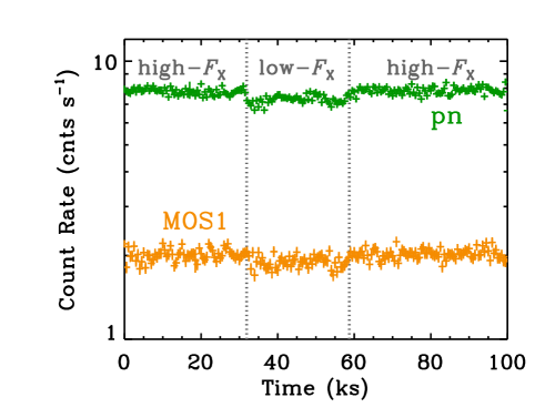
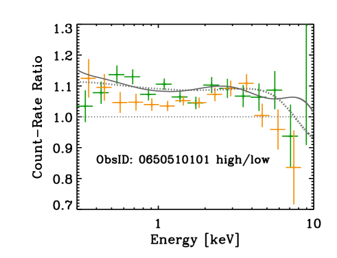
Figure 4: (a) Light curve for XMM-Newton ObsID: 060510101 for pn (green) and MOS1 (orange). The light curve for MOS2 is very similar to that of MOS1 shown here. A $\sim$6–7% “dip” in the light curves is observed between 31.9 and 58.9 ks, as denoted by the vertical lines with annotated periods of high and low flux. (b) Energy-dependent count-rate ratio between the high/low flux periods for pn (green) and combined MOS (orange) detectors. The differences in count-rate ratio are most obvious in the $\approx$0.3–4 keV range in energy, suggesting variations in the accretion disk itself are primarily responsible for the changes in flux, rather than in the Comptonization or absorption. Predicted ratios for the BH and NS baseline models are shown with the solid and dotted curves, respectively.

We chose to fit the spectra using both “BH” and “NS” models. For the BH models, we followed M11, who found two super-Eddington (TBABS $\times$ (DISKPBB + COMPTT) and TBABS $\times$ DISKPBB) and one sub-Eddington (TBABS $\times$ (DISKBB + COMPTT)) models provided good fits to the XMM-Newton data available at the time. Phenomenologically, the DISKPBB component serves as a model of the visible contribution of an advection dominated accretion disk, expected for accretion disks near the Eddington limit (e.g., Mineshige et al. 1994; Kubota & Makishima 2004). The model consists of an accretion disk with a radial temperature gradient, following $T(r)\propto r^{-p}$, where $p=0.75$ is the case of a standard thin disk and $p=$ 0.5–0.75 would be the case for an advection-dominant disk. The DISKBB model serves as a standard geometrically thin accretion disk (e.g., Kubota et al. 1998). The COMPTT model calculates the spectrum of seed photons as seen through a Comptonizing screen, which are assumed to be generated by some portion of the accretion disk. For all relevant fits, we establish a connection between the accretion disk and Comptonization components of the models by linking the seed-photon temperature of the COMPTT model to the temperature of the inner disk of either the DISKPBB or DISKBB models.

For the NS case, we fit the spectra to the super-Eddington model from W18 (TBABS $\times$ (DISKPBB + DISKBB + CUTOFF-PL)). Here, the accretion disk is thought to be composed of an inner advection dominant portion close to the NS (DISKPBB) and a standard outer portion (DISKBB). Following W18, we required that the DISKBB component yield an inner temperature below 1 keV to prevent swapping of temperatures with the hotter DISKPBB component. However, we found that the DISKBB component was not required in the case of M33 X-8; hereafter, we made use of the TBABS $\times$ (DISKPBB + CUTOFF-PL) for the NS case. The CUTOFF-PL component models Comptonization that is thought to arise from an accretion column falling onto the poles, within the magnetospheric radius. All known ULX pulsars have accretion columns that show broadly consistent spectral shapes (e.g., Brightman et al. 2016; W18). In our fitting, we followed the procedure of W18 and fixed the CUTOFF-PL shape to be the average of that measured from the three ULX pulsars known at the time (M82 X-2, NGC 7793 P13, and NGC 5907 ULX1). This model includes a photon-index of $\Gamma=0.5$ and cut-off energy of $E_{\_}{\rm cut}=8.1$ keV. In our procedure, we vary only the normalization of this component.

In Figure 3, we show the XMM-Newton pn and MOS, and NuSTAR FPMA and FPMB spectrum of M33 X-8, along with residuals to fits using the four models. In Table 2, we list the best fit model parameters and goodness-of-fit values. Thanks to the NuSTAR constraints, we can uniquely rule out both the pure advection dominated disk (DISKPBB) and sub-Eddington (DISKBB+COMPTT) BH models on the grounds of their poor fits (null-hypothesis probabilities of $P<6.7\times 10^{-9}$), particularly for the $E>$ 10 keV data. Instead, our data find the DISKPBB+COMPTT BH model and the DISKPBB + CUTOFF-PL NS model acceptable with null-hypothesis probabilities of 0.62 and 0.56, respectively (see Table 2).

For completeness, we also performed fits to additional basic spectral models that are often used to describe ULX spectra (e.g., POWERLAW, BKNPOWERLAW, DISKBB + POWERLAW, and DISKBB+CUTOFFPL). Fit parameters based on these models are provided in Appendix A. We find that most of these models were either poor fits to the data or unlikely on physical grounds. For example, the DISKBB + POWERLAW and DISKBB + CUTOFFPL only provide reasonable fits when the power-law components are significantly more luminous than the disk component at low energies ($\;\buildrel<\over{\sim}\;$2 keV). Such a solution is possible for sources where the seed photons arise from the Comtonizing source itself (e.g., an accretion column onto a pulsar). However, such sources are lower luminosity and exhibit obvious pulsations, which we do not find for X-8 (see $\S$3.4).

In the next section, we adopt the DISKPBB+COMPTT BH model and DISKPBB + CUTOFF-PL NS model when fitting archival XMM-Newton data; hereafter, we refer to these models as “baseline” BH and NS models, respectively. For the BH baseline model, we found than the COMPTT temperature ($kT_{\_}{\rm comp}$) and optical depth ($\tau$) were highly correlated and poorly constrained, even for our broad band fits. Our model suggests that a more optically-thick Comptonization component is slightly preferred. Therefore, when fitting to archival XMM-Newton data, we chose to fix $\tau=0.75$, near the best-fit value from the broad band fitting, and fit for $kT_{\_}{\rm comp}$.

3.2 Spectral Fits to Individual XMM-Newton Archival Observations

As discussed in $\S$2.2, a full list of the XMM-Newton archival data is provided in Table 1, with the timeline of X-8 source fluxes mapped in Figure 2. The fluxes reported are based on spectral fits to the pn data using our BH baseline model for each observation, with 90% uncertainties on the fluxes displayed. We note that the cross-calibration fluxes between instruments (pn, MOS, and NuSTAR detectors) is at the $\approx$7–10% level, suggesting that absolute calibration uncertainty is generally larger that the errors on the fluxes quoted here (e.g., Read et al. 2014; Madsen et al. 2017); however, the relative flux errors should be insensitive to this. The 0.3–10 keV flux has undergone little variation over the last 17 years of XMM-Newton observations, with the observational mean and standard deviation of $F_{\_}{\rm X}=(1.67\pm 0.11)\times 10^{-11}$ erg cm^-2 s^-1 ($L_{\_}{\rm X}=[1.38\pm 0.09]\times 10^{39}$ erg s^-1). Such a small scatter ($\approx$6%) in flux differs from the $\approx$30% reported by La Parola et al. (2015), which was based on fluxes from XMM-Newton, Chandra, Suzaku, BeppoSAX, and Swift. Their reported scatter is dominated by the previously reported XMM-Newton fluxes by M11, which are exclusively from MOS-camera data. The most extreme fluxes presented in the M11 study are based on XMM-Newton observations that were reported to have issues (e.g., slew failure, high levels of background radiation, and telemetry glitches). For example, M11 report that X-8 had an all time low MOS1 flux of $F_{\_}{\rm X}\approx 1.1\times 10^{-11}$ erg cm^-2 s^-1 during the 2003 Jan 22 observation (ObsID:0141980501); however, this observation was noted to suffer from a slew failure and resulted in large differences in calibration between cameras — the pn flux for X-8 during this observation is $F_{\_}{\rm X}\approx 1.8\times 10^{-11}$ erg cm^-2 s^-1. Using only the 14 Swift fluxes reported in Table 1 of La Parola et al. (2015), we obtain a scatter of only $\approx$7.7%, comparable to that reported here. Past monitoring from ROSAT has suggested that X-8 may exhibit a modulated period of $\approx$106 days with an amplitude of $\approx$20% (Dubus et al. 1997). The variability over the last 17 years is consistent with this amplitude.

Despite the small variations in flux, some spectral variations exist in the historical XMM-Newton observations of X-8, and these variations are broadly correlated with source flux. Using our BH and NS baseline models, we fit the data for each of the 17 XMM-Newton observations listed in Table 1 and attempted to isolate parameters of the model. The majority of our observations have relatively short exposures ($\;\buildrel<\over{\sim}\;$10 ks), and therefore the parameters of our models are only poorly constrained. Nonetheless, both BH and NS models provide a good-to-sufficient fit to the data (null-hypothesis probabilities of  0.02–0.75) for all ObsIDs, with the exception of ObsID: 0650510101 (null-hypothesis probability of $10^{-4}$), which constitutes one of the two longest observations in the archive (see Williams et al. 2015).

During ObsID: 0650510101, X-8 was reported by Sutton et al. (2013) to have a fractional variability of $F_{\_}{\rm var}=3.1\pm 0.3$% (calculated following Vaughan et al. 2003), which is $\approx$4 times larger than that found in the comparably long observation ObsID: 0650510201 ($F_{\_}{\rm var}=0.7\pm 0.5$%). In Figure 4$a$ we show the light curve for ObsID: 0650510101. It is clear that the large fractional variability is dominated by a $\approx$27 ks dip in the flux of X-8 that takes place $\approx$32 ks after the start of the observation. We investigated how the spectral properties of X-8 changed across the observation by extracting a “low-flux” spectrum at interval 31.9–58.9 ks and a “high-flux” spectrum, combining intervals 0–31.9 ks plus 58.9-100 ks (see Fig. 4$a$ annotations). The high flux 0.3–10 keV count rate is observed to be 7.2% and 6.4% higher than the low-flux count rate for the pn and mean MOS1+MOS2 detectors, respectively.

Table 3: Best Fit Parameters for Grouped Archival XMM-Newton Observations.

		ObsID 0650510101 Split		0.3–10 keV Flux Range (10-11 erg cm-2 s-1)
Parameter	Unit	(low-$F_{\_}{\rm X}$)	(high-$F_{\_}{\rm X}$)	($<$1.5)	(1.5–1.6)	(1.6–1.7)	($>$1.7)
Bin		…	…	1	2	3	4
$N_{\_}{\rm Bin}^{\dagger}$		1	1	1	4	6	5
BH Baseline Model
$N_{\_}{\rm H}$	1022 cm-2	0.157 $\pm$ 0.000	0.157${}_{\_}{-0.016}^{+0.030}$	0.161${}_{\_}{-0.014}^{+0.015}$	0.147${}_{\_}{-0.007}^{+0.008}$	0.166${}_{\_}{-0.014}^{+0.012}$	0.164${}_{\_}{-0.013}^{+0.017}$
$kT_{\_}{\rm in}$	keV	0.99${}_{\_}{-0.32}^{+0.25}$	0.72${}_{\_}{-0.08}^{+0.20}$	1.01${}_{\_}{-0.28}^{+0.55}$	0.84${}_{\_}{-0.05}^{+0.09}$	0.82${}_{\_}{-0.08}^{+0.13}$	0.94${}_{\_}{-0.15}^{+0.60}$
$p$		0.556 $\pm$ 0.006	0.547${}_{\_}{-0.033}^{+0.028}$	0.517${}_{\_}{-0.017}^{+0.016}$	0.556${}_{\_}{-0.056}^{+0.012}$	0.529${}_{\_}{-0.029}^{+0.020}$	0.537${}_{\_}{-0.037}^{+0.018}$
$(R_{\_}{\rm in}/D_{\_}{10})^{2}\cos\theta$		0.33${}_{\_}{-0.20}^{+1.02}$	1.04${}_{\_}{-0.53}^{+0.37}$	0.18${}_{\_}{-0.14}^{+0.42}$	0.55${}_{\_}{-0.14}^{+0.11}$	0.50${}_{\_}{-0.17}^{+0.15}$	0.34${}_{\_}{-0.29}^{+0.22}$
$kT_{\_}{\rm Comp}$	keV	$<$28.7	18.2${}_{\_}{-1.8}^{+5.5}$	$<$62.8	15.3${}_{\_}{-0.9}^{+1.0}$	14.0${}_{\_}{-1.9}^{+1.7}$	$<$3.1
Norm${}_{\_}{\rm Comp}$	10-4	0.30${}_{\_}{-0.28}^{+0.74}$	1.12${}_{\_}{-0.66}^{+0.39}$	0.18${}_{\_}{-0.14}^{+0.51}$	0.85${}_{\_}{-0.27}^{+0.18}$	1.08${}_{\_}{-0.35}^{+0.25}$	0.89${}_{\_}{-0.89}^{+0.34}$
$F_{\_}{\rm X}^{\rm disk}/F_{\_}{\rm X}$		0.75	0.55	0.67	0.64	0.60	0.67
$\chi^{2}/\nu(\nu)$		1.00 (984)	1.09 (1705)	1.03 (829)	1.03 (4955)	1.05 (3335)	1.10 (2577)
Null $P$		0.4820	0.0043	0.2413	0.0490	0.0233	0.0004
NS Baseline Model
$N_{\_}{\rm H}$	1022 cm-2	0.148 $\pm$ 0.000	0.148${}_{\_}{-0.009}^{+0.008}$	0.167${}_{\_}{-0.016}^{+0.006}$	0.142 $\pm$ 0.004	0.152${}_{\_}{-0.007}^{+0.006}$	0.160${}_{\_}{-0.008}^{+0.006}$
$kT_{\_}{\rm in}$	keV	1.11${}_{\_}{-0.06}^{+0.07}$	1.16${}_{\_}{-0.06}^{+0.07}$	1.24${}_{\_}{-0.14}^{+0.16}$	1.24 $\pm$ 0.03	1.36${}_{\_}{-0.08}^{+0.09}$	1.53${}_{\_}{-0.14}^{+0.12}$
$p$		0.561 $\pm$ 0.005	0.558${}_{\_}{-0.010}^{+0.012}$	0.502${}_{\_}{-0.002}^{+0.016}$	0.559 $\pm$ 0.005	0.545${}_{\_}{-0.007}^{+0.008}$	0.540${}_{\_}{-0.006}^{+0.005}$
$(R_{\_}{\rm in}/D_{\_}{10})^{2}\cos\theta$		0.21${}_{\_}{-0.05}^{+0.06}$	0.19${}_{\_}{-0.05}^{+0.06}$	0.06${}_{\_}{-0.01}^{+0.05}$	0.13${}_{\_}{-0.01}^{+0.02}$	0.09${}_{\_}{-0.02}^{+0.03}$	0.06${}_{\_}{-0.01}^{+0.03}$
Norm	10-4	2.13${}_{\_}{-0.50}^{+0.44}$	1.90${}_{\_}{-0.37}^{+0.34}$	2.73${}_{\_}{-0.47}^{+0.32}$	1.15${}_{\_}{-0.13}^{+0.12}$	0.87${}_{\_}{-0.44}^{+0.37}$	0.51${}_{\_}{-0.51}^{+0.68}$
$\chi^{2}/\nu(\nu)$		1.00 (985)	1.09 (1706)	1.04 (830)	1.03 (4956)	1.05 (3336)	1.10 (2578)
Null $P$		0.4837	0.0039	0.2331	0.0446	0.0202	0.0004

^† Number of XMM-Newton ObsIDs in a given bin.
Note—All quoted errors are at the 90% confidence level.

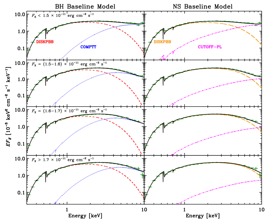
Figure 5: 0.3–10 keV XMM-Newton $EF_{\_}E$ spectra of M33 X-8, grouped by flux range for both our BH (left column) and NS (right column) baseline model. Best-fit models (black curves) were constructed using the joint spectral fitting technique described in $\S$3.3 and fit parameters are provided in Table 3. Green data points represent energy-binned average values and are plotted here for ease of viewing (these were not used in our spectral fitting). For the BH baseline models, the DISKPBB (red dashed curves) and COMPTT (blue dotted curves) contributions are shown, and for the NS baseline models, we display the DISKPBB (orange long-dashed curves) and CUTOFF-PL (magenta dot-dashed curves) contributions.

In Figure 4$b$, we show the high-to-low count-rate ratio as a function of energy. This ratio was computed by binning the spectra to evenly-divided $\log E$ bins. From these data, it appears that the predominant changes in the spectrum took place across the $\approx$0.3–4 keV energy range with the $\;\buildrel>\over{\sim}\;$4 keV data appearing to stay roughly constant between the two observations. This suggests that the changes in count rate were most likely associated with the accretion disk itself and not related to changes in absorption and Comptonization. To test this, we first performed fits to the high-flux spectrum using both our BH and NS baseline models. Fixing the absorption (TBABS) and Comptonization (either COMPTT or CUTOFF-PL) components, we then fit the low-flux spectrum, varying only the disk-component temperature, $p$ value, and normalization. Figure 4$b$ shows the predicted count-rate ratio as a function of energy for both the BH (solid curve) and NS (dotted curve) baseline models. Both BH and NS baseline models provided statistically acceptable fits to the data (see Table 3), suggesting indeed that the dip in flux can be described well by changes associated with the accretion disk. For the BH baseline model, the disk appears to be cooler and truncated (i.e., larger $R_{\_}{\rm in}$) in the low-flux case. The NS baseline model favors a slight cooling of the disk with the radial temperature profile becoming somewhat steeper (i.e., an increase in $p$).

3.3 Flux-Binned Spectral Fits to XMM-Newton Archival Observations

For the purpose of obtaining the best possible constraints on the spectral variations, we grouped the XMM-Newton X-8 spectra according to their 0.3–10 keV flux and performed joint spectral fitting of the data within a given bin. The observations were arbitrarily divided into four flux bins of $F_{\_}{\rm X}$/($10^{-11}$ erg cm^-2 s^-1) $<1.5$, 1.5–1.6, 1.6–1.7, and $>1.7$, which we hereafter refer to as bins 1, 2, 3, and 4, respectively. The bin assignments for the individual ObsIDs are listed in Table 1 and graphically illustrated in Figure 2 with the plotted circles colored according to their designated flux bin. Bins 1, 2, 3, and 4 respectively contain 1, 4, 6, and 5 unique XMM-Newton ObsIDs. In this exercise, we exclude ObsID: 0650510101, which was presented in the previous section, to provide unique results.

In our joint spectral fitting procedure, all data in a given bin were fit to our BH and NS baseline models to common (i.e., linked) model parameters, with the exception of a multiplicative constant model that was allowed to vary for each ObsID. In Table 3, we list the resulting best-fit parameters and goodness of fit for each of the four bins. For illustrative purposes, in Figure 5 we show binned $EF_{\_}E$ spectra for the four bins and the best-fit models, with model components separated. The stacked spectra shown in Figure 5 (green points) are average values with 1$\sigma$ errors on the mean of all data points within evenly-divided $\log E$ bins. Note that these stacked values were not used in our spectral fitting procedure and are simply shown here for illustrative purposes.

Both the BH and NS baseline models provide reasonable and nearly equivalent quality fits to the data; however, there is some tension in the fit quality for the data in the highest-flux bin (Bin 4), where the null-hypothesis probability is $0.0004$ for both models. Examination of the residuals to these fits suggests that there is likely some correlation between flux and the spectral shape within a given flux bin. As noted in $\S$3.2, all ObsIDs, except for ObsID 0650510101, can be fit well by these models on an individual basis. Thus, changes in the physical properties of the sources are likely responsible for the relatively low values of null-hypothesis probability here.

The best-fit parameters from our fits to the binned archival XMM-Newton data show only small changes over the range of X-ray fluxes covered. Nonetheless, some basic trends are apparent. In general, one can observe from Figure 5 that as $F_{\_}{\rm X}$ increases, the curvature of the higher-energy (i.e., $E\approx$ 2–10 keV) portion of the spectrum covered by XMM-Newton  increases, going from a relatively flat spectrum at $F_{\_}{\rm X}$/($10^{-11}$ erg cm^-2 s^-1) $<1.5$ to one that shows a clear $E\approx$ 1–3 keV turnover by $F_{\_}{\rm X}$/($10^{-11}$ erg cm^-2 s^-1) $>1.7$. The shape of the low-energy ($\;\buildrel<\over{\sim}\;$1 keV) spectrum, which we associate with the accretion disk, undergoes more subtle changes. Figure 6 graphically displays best-fit parameter values for the accretion disk versus $F_{\_}{\rm X}$ for both the BH and NS cases. Although subject to large uncertainties and some degeneracies between model parameters, we can use trends in the data here to make tentative interpretations of the nature of X-8. For guidance, in Figure 6, we show least squares regression lines fit to all the displayed data. For the BH baseline model, the flux-dependent variations in the spectrum of X-8 are consistent with the interpretation presented by M11, who proposed that as the accretion rate increases, winds from the disk become driven more effectively at larger radii due to the increased radiation pressure. The wind itself would provide a source of Comptonization This prediction leads to lower $kT_{\_}{in}$, larger inner radii, and a declining $F_{\_}{disk}/F_{\_}{\rm X}$ fraction with increasing $F_{\_}{\rm X}$. While the data do not show statistically significant correlations with $F_{\_}{\rm X}$, we do find that the preferred slopes from our least squares regression fits are consistent with this picture.

The NS baseline model case provides a somewhat different picture. Here X-8 can be interpreted as becoming more disk dominant with increasing flux, with the temperature (and possibly the size) of the accretion disk increasing. In comparison to other ULXs with broad band constraints from W18a, such behavior is similar to that observed for the ULX Holmberg IX X-1, which shows clear increase in curvature with increasing flux, most likely due to changes in the accretion disk (Luangtip et al. 2016; Walton et al. 2017). However, the known pulsar ULX, NGC 5907 ULX1 shows an increase in the high-energy component with increasing flux associated with the pulsar accretion column (W18a; Fürst et al. 2017). W18a speculate that the contrasting behavior of Holmberg IX X-1 with that of NGC 5907 ULX1 could be an indication of differing compact-object types (i.e., BH vs. NS) or viewing angles.

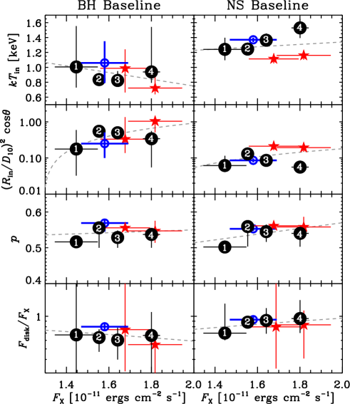
Figure 6: Accretion disk parameters versus 0.3–10 keV flux ($F_{\_}{\rm X}$) for the BH (left column) and NS (right column) baseline models. These plots include, from top to bottom, the inner accretion disk temperature, radius, temperature profile index $p$, and the fraction of the total flux attributed to the accretion disk. Fit results are shown for our nearly simultaneous NuSTAR plus XMM-Newton exposure (open blue circle), the high/low flux intervals of ObsID 0650510101 (red stars), and $F_{\_}{\rm X}$-divided bins (black circles with annotated bin number). Least squares regression lines (dotted gray lines) fit to all data points in each panel are included as indicators of potential trends with $F_{\_}{\rm X}$.

3.4 Search for Pulsations

While our spectral analyses provide new constraints on the nature of accretion in M33 X-8, we cannot draw firm conclusions about the nature of the compact object itself. Given the discovery of pulsations in other ULXs, we searched the 3–20 keV light curves of the two NuSTAR epochs that contain X-8 (ObsIDs 50310002001 and 50310002003) to test whether the hard component is pulsating.

All photon arrival times were converted to barycentric dynamical time. Following the methodology of Yang et al. (2017) in search of periodic pulsations, we constructed Lomb-Scargle periodograms for the whole observing time and searched for spin periods in the range 0.15–200476 s. No significant pulsations were detected in the second NuSTAR epoch. However, a periodic signal was independently detected in both telescopes FPMA ($769.42\pm 4.87$ s) and FPMB ($724.82\pm 5.22$ s) during the first NuSTAR epoch (ObsID 50310002001), but the periods are statistically inconsistent. This should not be the case if a true periodic signal was emanating from the source, given that the source was observed simultaneously by these two telescopes.

The discrepancy between these candidate period values is not explained by any typical observing window function effect, but could be due to the presence of red noise that behaves as a broken power law in the light curve of M33 X-8. The break frequency could be broadly picked up as a single periodicity by the Lomb-Scargle algorithm, resulting in relatively similar but statistically distinct values being independently detected by the FPMA and FPMB telescopes.

Due to the inconsistency between period values and lack of any physically compelling explanation for the discrepancy, we cannot claim to have found a significant, coherent signal in the NuSTAR light curves searched in our study.

4 Discussion and Conclusions

The broad band spectra and light curves of M33 X-8, presented in $\S$3, provide updated constraints on the nature of this source. Thanks to the nearly simultaneous XMM-Newton and NuSTAR observational constraints, we can now rule out the previously acceptable sub-Eddington (DISKBB + COMPTT) and pure advection-dominated disk (DISKPBB) models for X-8. Instead, we find that the constraints are consistent with more recent models of super-Eddington accretion onto either a BH or NS, albeit with no clear preference for a BH or NS accretor.

While preparing this manuscript, a paper on M33 X-8 by Krivonos et al. (2018) was published that made use of the NuSTAR data that we present here, in combination with Swift archival data, to provide lower-energy constraints. In general, we find basic agreement between our spectral constraints, and those of Krivonos et al. (2018), with the exception that their data allows for an acceptable fit using the DISKBB + COMPTT, which prompted them to claim that M33 X-8 is most likely a BH XRB in a very high state. We attribute the difference in findings to their use of archival Swift data, which spans a range of fluxes and provides weaker spectral constraints on the data. Our use of nearly simultaneous, high-S/N XMM-Newton and NuSTAR data is therefore crucial for ruling out this model. Here, we prefer an interpretation in which M33 X-8 is in an accretion state in which the structure of the disk has been modified by advection, as required by our broad band fits. Such sources have been purported to be likely BH XRBs due to their similarities with known Galactic BH XRBs (Sutton et al. 2017); however, we are unable to clearly distinguish between a NS or BH nature of the accretor.

For the BH interpretation, the data presented here are consistent with past phenomenological models of ULXs, in which an advection-dominated disk appears cooler and truncated at relatively high fluxes, potentially due to the increase in outflowing material from the inner portions of the disk. Here, the outflowing material provides both obscuration of the hot inner disk and Comptonization (see $\S\S$5.3 and 5.4 of Kaaret et al. 2017 for a comprehensive description of this model). In this context, the increase in spectral curvature at $\;\buildrel>\over{\sim}\;$3 keV with increasing flux is expected to be due to the Comptonization component becoming cooler and possibly more optically thick. Other variable ULXs have been reported to show this same type of behavior, when analyzing 0.3–10 keV spectra (most notably with XMM-Newton). For example, a recent observation of a drop in the flux of ULX IC 342 X-1 showed a shift in the spectral turnover to higher energies as the luminosity decreased by a factor of $\sim$2 (Shidatsu et al. 2017). Similarly, Ho IX X-1 has shown similar spectral changes over a broad range of fluxes. For this source, the spectrum transitions smoothly from a relatively flat high-energy component at $\;\buildrel>\over{\sim}\;$2 keV for low luminosities to a highly curved component at the highest luminosities of the source (Luangtip et al. 2016).

The above spectral behavior can also be interpreted as changes in the accretion disk itself. In the right column of Figure 5, we showed, using our NS baseline model, that the 0.3–10 keV spectral variability of M33 X-8 could be modeled well by an advection-dominated disk increasing in temperature with increasing flux. In this scenario, the increased importance of the accretion disk relative to the high-energy Comptonization component is what leads to spectral curvature at $\;\buildrel>\over{\sim}\;$3 keV, instead of the Comptonization itself. The Comptonization component itself, which is modeled here as an accretion column onto the NS, would have very minor contributions to the 0.3–10 keV spectra, and is thus poorly constrained. Furthermore, W18a showed that both Ho IX X-1 and IC 342 X-1, when analyzed using broad band (0.3–30 keV) spectral data, can also be fit well using their NS-based two-component thermal model (DISKPBB + DISKBB) plus Comptonization (CUTOFF-PL) model. They too find that for Ho IX X-1, for which broad band observations are available for different flux states, the enhancement in spectral curvature with increasing flux can be explained by a rise in the contribution of the DISKPBB component, with little change in Comptonization.

It is important to point out here that the changes in the broad band spectra of Ho IX X-1, as modeled by W18a, differ from those of the known pulsating ULX NGC 5907 ULX1, which was shown to have strong variations in the hard Comptonization component, associated with the accretion column of the NS. This difference in behavior could be an indicator of a BH nature for Ho IX X-1, and perhaps by extension, IC 342 X-1 and M33 X-8. Although our NS baseline model was motivated to test whether an accretion column model from W18a was appropriate for NSs was acceptable, this model can easily be adapted to BHs by replacing the accretion column with an optically thin disk wind.

Unfortunately, we are unable to determine the nature of the compact object in M33 X-8 in this study. Part of the difficulty is that, for the NS baseline model, the Comptonization component is modeled to be quite weak relative to the disk, similar to that observed for high-luminosity Galactic accreting pulsars (Yang et al. 2018). Thus, if M33 X-8 contains a pulsating NS, pulsations would likely be weak and difficult to detect, even with broad band data, unless the NS were to go into a bright state, similar to that found in NGC 5907 ULX1. On the other hand, significant headway can be made in understanding the nature of the accretion disk and Comptonization components by obtaining additional broad band spectra of X-8 in various flux states. When using the archival XMM-Newton data to interpret changes in the spectrum, we find degeneracies between the BH and NS models, which could be broken using data above 10 keV. In particular, future XMM-Newton and NuSTAR observations of X-8 in low ($F_{\_}{\rm X}<1.5\times 10^{-11}$ erg cm^-2 s^-1) and high ($F_{\_}{\rm X}>1.7\times 10^{-11}$ erg cm^-2 s^-1) states would allow these degeneracies to be addressed better.

Appendix A Supplemental Fits to Nearly Simultaneous NuSTAR plus XMM-Newton Observation

As an extension to the spectral fits presented in $\S$3.1, Table A1 provides parameters and goodness of fit information for four alternative model fits to the nearly simultaneous NuSTAR plus XMM-Newton observations.

Table A1: Supplemental Best fit parameters for Nearly-Simultaneous NuSTAR plus XMM-Newton Observation.

Parameter	Unit	Value
TBABS $\times$ POWERLAW
$N_{\_}{\rm H}$	1022 cm-2	0.28
$\Gamma$		2.49
$N_{\_}{\rm pow}$	keV-1 cm-2 s-1 at 1 keV	$6.8\times 10^{-3}$
$\chi^{2}/\nu(\nu)$		3.63 (1715)
Null $P$		0
TBABS $\times$ BKNPOWER
$N_{\_}{\rm H}$	1022 cm-2	$0.185\pm 0.005$
$\Gamma_{\_}1$		$1.97\pm 0.02$
$E_{\_}{\rm break}$		$3.70\pm 0.08$
$\Gamma_{\_}2$		$3.40\pm 0.04$
$N_{\_}{\rm bknpow}$	keV-1 cm-2 s-1 at 1 keV	$(4.77\pm 0.08)\times 10^{-3}$
$\chi^{2}/\nu(\nu)$		1.08 (1713)
Null $P$		0.01
TBABS $\times$ (DISKBB + POWERLAW)
$N_{\_}{\rm H}$	1022 cm-2	$0.207\pm 0.007$
$kT_{\_}{\rm in}$	keV	$1.21\pm 0.02$
$(R_{\_}{\rm in}/D_{\_}{10})^{2}\cos\theta$		$0.22\pm 0.02$
$\Gamma$		$2.60\pm 0.03$
$N_{\_}{\rm pow}$	keV-1 cm-2 s-1 at 1 keV	$(3.3\pm 0.2)\times 10^{-3}$
$\chi^{2}/\nu(\nu)$		1.01 (1713)
Null $P$		0.33
TBABS $\times$ (DISKBB + CUTOFFPL)
$N_{\_}{\rm H}$	1022 cm-2	$0.167\pm 0.008$
$kT_{\_}{\rm in}$	keV	$1.14\pm 0.03$
$(R_{\_}{\rm in}/D_{\_}{10})^{2}\cos\theta$		$0.24_{\_}{-0.02}^{+0.03}$
$\Gamma$		$2.15\pm 0.13$
High-$E$ Cut	keV	$11.8_{\_}{-2.8}^{+4.9}$
$N_{\_}{\rm cuttoffpl}$	keV-1 cm-2 s-1 at 1 keV	$(3.2\pm 0.2)\times 10^{-3}$
$\chi^{2}/\nu(\nu)$		0.99 (1712)
Null $P$		0.56

Note—All quoted errors are at the 90% confidence level. Given the very poor fit provided by the TBABS $\times$ POWERLAW model, errors are not reported.

References

- Abramowicz et al. (1988) Abramowicz, M. A., Czerny, B., Lasota, J. P., & Szuszkiewicz, E. 1988, ApJ, 332, 646
- Arnaud (1996) Arnaud, K. A. 1996, Astronomical Data Analysis Software and Systems V, 101, 17
- Bachetti et al. (2014) Bachetti, M., Harrison, F. A., Walton, D. J., et al. 2014, Nature, 514, 202
- Bhardwaj et al. (2016) Bhardwaj, A., Kanbur, S. M., Macri, L. M., et al. 2016, AJ, 151, 88
- Brightman et al. (2016) Brightman, M., Harrison, F., Walton, D. J., et al. 2016, ApJ, 816, 60
- Carpano et al. (2018) Carpano, S., Haberl, F., Maitra, C., & Vasilopoulos, G. 2018, MNRAS, 476, L45
- Davis et al. (2017) Davis, B. L., Graham, A. W., & Seigar, M. S. 2017, MNRAS, 471, 2187
- Dickey & Lockman (1990) Dickey, J. M., & Lockman, F. J. 1990, ARA&A, 28, 215
- Done et al. (2004) Done, C., Wardziński, G., & Gierliński, M. 2004, MNRAS, 349, 393
- Dotan & Shaviv (2011) Dotan, C., & Shaviv, N. J. 2011, MNRAS, 413, 1623
- Dubus et al. (1997) Dubus, G., Charles, P. A., Long, K. S., & Hakala, P. J. 1997, ApJ, 490, L47
- Fürst et al. (2016) Fürst, F., Walton, D. J., Harrison, F. A., et al. 2016, ApJ, 831, L14
- Fürst et al. (2017) Fürst, F., Walton, D. J., Stern, D., et al. 2017, ApJ, 834, 77
- Gabriel et al. (2004) Gabriel, C., Denby, M., Fyfe, D. J., et al. 2004, in ASP Conf. Ser. 314, Astronomical Data Analysis Software and Systems (ADASS) XIII, ed. F. Ochsenbein, M. G. Allen, & D. Egret (San Francisco, CA: ASP), 759
- Garofali et al. (2018) Garofali, K., Williams, B. F., Hillis, T., et al. 2018, MNRAS, 479, 3526
- Gebhardt et al. (2001) Gebhardt, K., Lauer, T. R., Kormendy, J., et al. 2001, AJ, 122, 2469
- Gladstone et al. (2009) Gladstone, J. C., Roberts, T. P., & Done, C. 2009, MNRAS, 397, 1836
- Israel et al. (2017) Israel, G. L., Belfiore, A., Stella, L., et al. 2017, Science, 355, 817
- Jourdain et al. (2017) Jourdain, E., Roques, J.-P., & Rodi, J. 2017, ApJ, 834, 130
- Kaaret et al. (2017) Kaaret, P., Feng, H., & Roberts, T. P. 2017, ARA&A, 55, 303
- King (2009) King, A. R. 2009, MNRAS, 393, L41
- King & Lasota (2016) King, A., & Lasota, J.-P. 2016, MNRAS, 458, L10
- King et al. (2017) King, A., Lasota, J.-P., & Kluźniak, W. 2017, MNRAS, 468, L59
- Koliopanos et al. (2017) Koliopanos, F., Vasilopoulos, G., Godet, O., et al. 2017, A&A, 608, A47
- Krivonos et al. (2018) Krivonos, R., Sazonov, S., Tsygankov, S., & Poutanen, J. 2018, arXiv:1807.10427
- Kubota et al. (1998) Kubota, A., Tanaka, Y., Makishima, K., et al. 1998, PASJ, 50, 667
- Kubota & Makishima (2004) Kubota, A., & Makishima, K. 2004, ApJ, 601, 428
- La Parola et al. (2015) La Parola, V., D’Aí, A., Cusumano, G., & Mineo, T. 2015, A&A, 580, A71
- Long et al. (1981) Long, K. S., Dodorico, S., Charles, P. A., & Dopita, M. A. 1981, ApJ, 246, L61
- Long et al. (2002) Long, K. S., Charles, P. A., & Dubus, G. 2002, ApJ, 569, 204
- Luangtip et al. (2016) Luangtip, W., Roberts, T. P., & Done, C. 2016, MNRAS, 460, 4417
- Madsen et al. (2017) Madsen, K. K., Beardmore, A. P., Forster, K., et al. 2017, AJ, 153, 2
- Middleton et al. (2011) Middleton, M. J., Sutton, A. D., & Roberts, T. P. 2011, MNRAS, 417, 464 (M11)
- Mineshige et al. (1994) Mineshige, S., Hirano, A., Kitamoto, S., Yamada, T. T., & Fukue, J. 1994, ApJ, 426, 308
- Mineshige et al. (2000) Mineshige, S., Kawaguchi, T., Takeuchi, M., & Hayashida, K. 2000, PASJ, 52, 499
- Mushtukov et al. (2017) Mushtukov, A. A., Suleimanov, V. F., Tsygankov, S. S., & Ingram, A. 2017, MNRAS, 467, 1202
- Pietsch et al. (2004) Pietsch, W., Misanovic, Z., Haberl, F., et al. 2017, A&A, 426, 11
- Pintore et al. (2017) Pintore, F., Zampieri, L., Stella, L., et al. 2017, ApJ, 836, 113
- Poutanen et al. (2007) Poutanen, J., Lipunova, G., Fabrika, S., Butkevich, A. G., & Abolmasov, P. 2007, MNRAS, 377, 1187
- Read et al. (2014) Read, A. M., Guainazzi, M., & Sembay, S. 2014, A&A, 564, A75
- Revnivtsev et al. (2002) Revnivtsev, M., Gilfanov, M., Churazov, E., & Sunyaev, R. 2002, A&A, 391, 1013
- Shidatsu et al. (2017) Shidatsu, M., Ueda, Y., & Fabrika, S. 2017, ApJ, 839, 46
- Strüder et al. (2001) Strüder, L., Briel, U., Dennerl, K., et al. 2001, A&A, 365, L18
- Sutton et al. (2013) Sutton, A. D., Roberts, T. P., & Middleton, M. J. 2013, MNRAS, 435, 1758
- Sutton et al. (2017) Sutton, A. D., Swartz, D. A., Roberts, T. P., et al. 2017, ApJ, 836, 48
- Tsygankov et al. (2017) Tsygankov, S. S., Doroshenko, V., Lutovinov, A. A., et al. 2017, A&A, 605, A39
- Tüllmann et al. (2011) Tüllmann, R., Gaetz, T. J., Plucinsky, P. P., et al. 2011, ApJS, 193, 31
- Turner et al. (2001) Turner, M. J. L., Abbey, A., Arnaud, M., et al. 2001, A&A, 365, L27
- Vaughan et al. (2003) Vaughan, S., Edelson, R., Warwick, R. S., & Uttley, P. 2003, MNRAS, 345, 1271
- Walton et al. (2017) Walton, D. J., Fürst, F., Harrison, F. A., et al. 2017, ApJ, 839, 105
- Walton et al. (2018) Walton, D. J., Fürst, F., Heida, M., et al. 2018a, ApJ, 856, 128 (W18)
- Walton et al. (2018) Walton, D. J., Fürst, F., Harrison, F. A., et al. 2018b, MNRAS, 473, 436
- Wiktorowicz et al. (2017) Wiktorowicz, G., Sobolewska, M., Lasota, J.-P., & Belczynski, K. 2017, ApJ, 846, 17
- Williams et al. (2015) Williams, B. F., Wold, B., Haberl, F., et al. 2015, ApJS, 218, 9
- Wilson-Hodge et al. (2018) Wilson-Hodge, C. A., Malacaria, C., Jenke, P. A., et al. 2018, ApJ, 863, 9
- Yang et al. (2017) Yang, J., Laycock, S. G. T., Christodoulou, D. M., et al. 2017, ApJ, 839, 119
- Yang et al. (2018) Yang, J., Zezas, A., Coe, M. J., et al. 2018, MNRAS, 479, L1