LFTC-18-12/33

Laboratório de Física Teórica e Computacional-LFTC
Universidade Cruzeiro do Sul, 015060-000, São Paulo, SP, Brazil

Unambiguous Extraction of the Electromagnetic Form Factors for Spin-1 Particles on the Light-Front

Abstract

The electromagnetic form factors of a composite vector particle within the light-front formulation of the Mandelstam formula is investigated. In order to extract the form factors from the matrix elements of the plus component of the current in the Drell-Yan frame, where the momentum transfer is chosen such that $q^{+}=q^{0}+q^{3}=0$, one has in principle the freedom to choose between different linear combinations of matrix elements of the current operator. The different prescriptions to calculate the electromagnetic form factors, $G_{0},G_{1}$ and $G_{2}$, i.e.; charge form factor, magnetic and quadrupole respectively. If the covariance is respected, all prescriptions give the same results; misfortune, is not the situation; the light-front approach produce different results, which depend of the prescriptions as utilized to extract the electromagnetic form factors in the case of the spin-1 particles. The main differences of the prescriptions appear because of the light-front matrix elements of the electromagnetic current are contaminated by the zero-modes contributions to the same with the plus component of the matrix elements of the electromagnetic current. However, the Inna Grach prescription is immune to the zero-modes contributions to the electromagnetic current, then the electromagnetic form factors extracted with that prescriptions do not have zero-modes contribution and give the same result compared with the instant form quantum field theory. Another’s prescriptions with the light-front approach are contaminated by the zero-modes contributions to the matrix elements of the electromagnetic current with the plus component of the current. With some relations between the electromagnetic matrix elements of the electromagnetic current $J^{+}_{ji}$, as demonstrated analytical here, it was possible to calculate the electromagnetic form factors for spin-1 particles without zero-modes or non-valence contributions.

Introduction: The light-front quantum field theory (LFQFT), is a natural theory to describe composite systems, like meson or baryons [1], and the Fock amplitudes of the eigenstates the LF Hamiltonian reflects the complex structure of the hadron obtained with the fundamental interactions from Quantum Chromodynamics. In respect to the phenomenological success of this approach, we should add that it produced results comparable to other approaches for hadron structure, for example, Schwinger-Dyson methods  [2, 3, 4], QCD sum rules [5, 6, 7, 8, 9, 11, 12], AdS/QCD frameworks [13], Effective Field Theory [14], and also covariant light-front dynamics [15, 16] and recently the point-form quantum mechanics [17]. On the hand, in LFQFT, the vacuum is trivial and the kinematical group contains Lorentz transformations  [1, 18]. This is an advantage over the usual formalism and allows a great simplification in calculations of bound states [16, 19]. However, some problems with that approach remain, the most critical point is the loss of covariance in some physical processes [20, 21, 22, 23, 24, 25]. In order to restore the full covariance of the electromagnetic current, besides the valence component, we need to add the non-valence contributions or zero-modes to the matrix elements of the electromagnetic current to keep the full covariance [20, 22, 23, 24, 26]. Moreover, the light-front quantum field theory, is the natural theory to describe hadronic bound states, like pseudoscalar particles [15, 23, 27, 28, 29, 30, 31, 32, 33], or spin half particles [34]. As well, in the last years, some works are dedicate to spin-1 particles, with different approaches [5, 8, 9, 10, 24, 31, 35, 36, 37, 38, 39, 40, 41, 42, 43, 44, 45, 46, 47, 48, 49, 50, 51]. In addition, some studies of the hadronic properties in the nuclear medium was made in the references [52, 53, 54, 55, 56, 57, 58, 59].

The vertex model and electromagnetic current. The vertex model for the spinor structure of the composite spin-one particle, ($m_{v}-q\bar{q}$), comes from the model proposed in [20]:

$$\Gamma^{\mu}(k,p)=\gamma^{\mu}-\frac{m_{v}}{2}\left(k^{\mu}+k^{\prime\mu}\right)\,D^{-1}_{v}(k)~{},$$ (1)

where $m_{v}$ is the vector spin-1 particle mass, $D_{v}(k)=(p\cdot k+m_{v}m-\imath\epsilon)$ and $k^{\prime}=k-p$.

The Mandelstam formula to compute the electromagnetic form factors of the vector particle from the plus component of the current, $J^{+}=J^{0}+J^{3}$, is given by:

$$J^{+}_{ji}=\imath\int\frac{d^{4}k}{(2\pi)^{4}}\frac{Tr\left[\Gamma\Gamma\right]^{+}_{ji}\,\Lambda(k,p_{f})\,\Lambda(k,p_{i})}{((k-p_{i})^{2}-m^{2}+\imath\epsilon)(k^{2}-m^{2}+\imath\epsilon)((k-p_{f})^{2}-m^{2}+\imath\epsilon)},$$ (2)

where, $\gamma^{+}=\gamma^{0}+\gamma^{3}$ is the Dirac matrix, the four-vector are $a^{\mu}=(a^{+}=a^{0}+a^{3},a^{-}=a^{0}-a^{3},a_{1},a_{2})=(a^{+},a^{-},\vec{a}_{\perp})$, and $a.b=\frac{a^{+}b^{-}+a^{-}b^{+}}{2}-\vec{a}_{\perp}\vec{b}_{\perp}$, following the Light-front formalism [1]. The integral for the matrix elements of the current above with the Light-front coordinates is $d^{4}k=\frac{1}{2}d^{2}k_{\perp}dk^{+}dk^{-}$.

In the equation above, the numerator is given by the Dirac trace:

$$Tr\left[\Gamma\Gamma\right]^{+}_{ji}=Tr\left[\epsilon_{j}\cdot\Gamma(k,p_{f})(\hbox to0.0pt{/\hss}k-\hbox to0.0pt{/\hss}p_{f}+m)\gamma^{+}(\hbox to0.0pt{/\hss}k-\hbox to0.0pt{/\hss}p_{i}+m)\epsilon_{i}\cdot\Gamma(k,p_{i})(\hbox to0.0pt{/\hss}k+m)\right].$$ (3)

The regularization function in Eq. (2), is $\Lambda(k,p)=N/[(k-p)^{2}-m^{2}_{R}+\imath\epsilon]^{2}$, which is chosen to turn the loop integration finite [20]. In the present work, we adopt the Breit-frame with $q^{+}=q^{0}+q^{3}=0$, $q_{y}=0$ and $q_{x}\neq 0$ to compute the matrix elements of the current. The Cartesian four-vector polarizations of the massive vector particle, in the instant form representation ($x^{\mu}=(t,x,y,z)$) in the chosen frame, are given by:

$$\epsilon^{\mu}_{x}=(-\sqrt{\eta},\sqrt{1+\eta},0,0),\,\,\epsilon_{y}^{\mu}=(0,0,1,0),\,\,\epsilon_{z}^{\mu}=(0,0,0,1),$$ (4)

for the initial state and the final state,

$$\epsilon^{{}^{\prime}\mu}_{x}=(\sqrt{\eta},\sqrt{1+\eta},0,0),\,\,\epsilon_{y}^{{}^{\prime}\mu}=(0,0,1,0),\,\,\epsilon_{z}^{{}^{\prime}\mu}=(0,0,0,1),$$ (5)

where $\eta=-\frac{q^{2}}{4m^{2}_{v}}$. Given the polarizations vectors, the quantities $G_{0}$, $G_{1}$ and $G_{2}$, namely the charge, magnetic and quadrupole form factors are found as linear combinations of the matrix elements of the electromagnetic current (see e.g. [20, 60]). The constraints of covariance, parity and current conservation restrict the number of form factors for the vector particle to three. From these requirements, the non-vanishing matrix elements are $J^{+}_{xx}$, $J^{+}_{yy}$, $J^{+}_{zz}$ and $J^{+}_{zx}=-J^{+}_{xz}$, therefore one relation exists among them, namely the angular condition expressed as [61, 64]:

$$\Delta(q^{2})=\left(J^{+}_{yy}-J^{+}_{zz}\right)\left(1+\eta\right)=0.$$ (6)

If the angular condition is violated, the different prescriptions in the literature [61, 64, 62, 63], used to obtain the form factors produces different results (see e.g. [20]). The source of this problem was traced back to missing zero-mode contributions to the matrix elements of the current [21, 22, 65]. In a recent paper [26], was analyzed the contributions of zero modes to the matrix elements of plus component of the electromagnetic current,  $J^{+}$, coming from non-vanishing pair production amplitudes (Z-diagrams) in the limit of $q^{+}\to 0_{+}$, where it was employed a symmetric form of the vector particle vertex, namely:

$$\Lambda_{s}^{\mu}(k,p)=\Gamma^{\mu}(k,p)\,\Lambda(k,p)+\left[k\leftrightarrow-k^{\prime}\right],$$ (7)

which generalizes the vertex function, Eq.(1). The conclusion of [26] for the zero-mode contributions to the matrix elements of the current can be summarized in the following relations:

$$J^{+Z}_{yy}=0,\,\,J^{+Z}_{xx}=-\eta\ J^{+Z}_{zz}\,\,\text{and}\,\,J^{+Z}_{zx}=-\sqrt{\eta}\ J^{+Z}_{zz},\,\,$$ (8)

where the last two can be computed solely from the valence contributions as:

$$J^{+Z}_{zz}=J^{+V}_{yy}-J^{+V}_{zz},$$ (9)

which is a consequence of the angular condition, Eq. (6), fulfilled by the covariant and current conserving model given by the vertex function, Eq. (7).

The final relations for the matrix elements of the plus component of the current, can be computed solely in terms of valence matrix elements:

$$J^{+}_{xx}=J^{+V}_{xx}-\eta(J^{+V}_{yy}-J^{+V}_{zz})\,\,\text{and}\,\,J^{+}_{zx}=J^{+V}_{zx}-\sqrt{\eta}(J^{+V}_{yy}-J^{+V}_{zz}),$$ (10)

these expressions ensure that the zero-modes are taken into account for the vertex model, Eq. (7). The resulting evaluation of the form factors with the above matrix elements are in agreement with a direct covariant calculation, namely, without resorting to the projection onto the light-front. The advantage of this strategy is the possibility to apply the relations given in the Eq. (10) to compute the form factors of composite vector particles for any valence wave function model.

The relations between the matrix elements of the current in the Cartesian and, in the light-front spin (helicity) basis, $I^{+}_{m^{\prime}m}$ are given by [20, 64]:

$$I^{+}_{11}=\frac{J^{+}_{xx}+(1+\eta)J^{+}_{yy}-\eta J^{+}_{zz}+2\sqrt{\eta}J^{+}_{zx}}{2(1+\eta)},$$

$$I^{+}_{10}=\frac{\sqrt{2\eta}J^{+}_{xx}+\sqrt{2\eta}J^{+}_{zz}+\sqrt{2}(\eta-1)J^{+}_{zx}}{2(1+\eta)},$$

$$I^{+}_{1-1}=\frac{-J^{+}_{xx}+(1+\eta)J^{+}_{yy}+\eta J^{+}_{zz}-2\sqrt{\eta}J^{+}_{zx}}{2(1+\eta)},$$

$$I^{+}_{00}=\frac{-\eta J^{+}_{xx}+J^{+}_{zz}+2\sqrt{\eta}J^{+}_{zx}}{(1+\eta)}\ .$$ (11)

The elimination of zero-modes for the matrix elements of the current $I^{+}_{m^{\prime}m}$ through the relations, Eq’s. (8), (9) and (10), leads to the following:

$$I^{+Z}_{11}=0,\,\,\,I^{+Z}_{10}=0,\,\,\,I^{+Z}_{1-1}=0,$$ (12)

and

$$I^{+Z}_{00}=(1+\eta)J^{+Z}_{zz}=(1+\eta)\left(J^{+V}_{yy}-J^{+V}_{zz}\right),$$ (13)

showing only the $I^{+Z}_{00}$ component of the electromagnetic current has a non-zero contribution from the zero-mode [26]. The relation, Eq. (13), is also associated with the fulfillment of the angular condition,

$$\Delta(Q^{2})=(1+2\eta)I^{+}_{11}+I^{+}_{1-1}-\sqrt{8\eta}I^{+}_{10}-I^{+}_{00}~{},$$ (14)

where the matrix elements of $I^{+}_{11}$, $I^{+}_{1-1}$, and $I^{+}_{10}$, due to Eq. (12), are computed only from the valence terms. After the inclusion the zero modes, or the non-valence contributions, the angular condition above, results is zero, $\Delta(Q^{2})=0$. These results was also found in the reference [22] for the particular case of $\gamma^{\mu}$ vertex coupling for the $q\bar{q}$ pair to the $\rho$-meson for a smeared photon-vertex and further explored in [21] for the vector particle coupling to the quarks given by Eq. (1).

In the next section, we demonstrate for all prescriptions utilized in the literature to extract the form factors for spin-1 particles and with the plus component of the electromagnetic current, $J^{+}$,  in the Breit-Frame and Drell-Yan condition are equivalent to each other if the relations, Eq. (10), are used.

Light-Front Prescriptions for the electromagnetic form factors. Therefore, out of the four matrix elements it is possible to combine them current in different ways. Because this, the linear combinations utilized in order to extract the electromagnetic form factors from electromagnetic matrix elements of the current [20, 60, 64] is not unique; but this leads us to make a choose which of the current matrix element eliminate, and used to the extract the electromagnetic form factors, $G_{0},G_{1}$ and $G_{2}$, then we have different prescriptions to extracted the electromagnetic form factors [20, 60]. Following the Ref. [20], the four prescriptions in the literature are written below in the instant form, (IF), basis of spin and with the light-front basis [20, 60].

In the reference [61], the authors eliminate the $I^{+}_{00}$ component of the electromagnetic current in the light-front spin basis, and writing in the Cartesian basis also [20],

$$G_{0}^{GK} = \frac{1}{3}[(3-2\eta)I^{+}_{11}+2\sqrt{2\eta}I^{+}_{10}+I^{+}_{1-1}]$$

$$= \frac{1}{3}[J_{xx}^{+}+(2-\eta)J_{yy}^{+}+\eta J_{zz}^{+}],$$

$$G_{1}^{GK} = 2[I^{+}_{11}-\frac{1}{\sqrt{2\eta}}I^{+}_{10}]=J_{yy}^{+}-J_{zz}^{+}-\frac{J_{zx}^{+}}{\sqrt{\eta}},$$

$$G_{2}^{GK} = \frac{2\sqrt{2}}{3}[\sqrt{2\eta}I^{+}_{10}-\eta I^{+}_{11}-I^{+}_{1-1}]=\frac{\sqrt{2}}{3}[J_{xx}^{+}-(1+\eta)J_{yy}^{+}+\eta J_{zz}^{+}]~{}.$$ (15)

With the relations given by the Eq.(8) and Eq.(10), and after made the substitution in expressions for the electromagnetic form factors below [61]:

$$G^{GK\ (+Z)}_{0} = \frac{1}{3}\left[J_{xx}^{(+Z)}+\eta J_{zz}^{+Z}\right]=\frac{1}{3}\left[-\eta J_{zz}^{+Z}+\eta J_{zz}^{+Z}\right]=0,$$

$$G_{1}^{GK~{}(+Z)} = \left[-J_{zz}^{+Z}[gg]-\frac{J_{zx}^{+Z}}{\sqrt{\eta}}\right]=-J_{zz}^{+Z}+\sqrt{\eta}\frac{J_{zz}^{+Z}}{\sqrt{\eta}}=0,$$

$$G_{2}^{GK\ (+Z)} = \frac{\sqrt{2}}{3}\left(J_{xx}^{+Z}+\eta J_{zz}^{+Z}\right)=\frac{\sqrt{2}}{3}\left[-\eta J_{zz}^{+}+\eta J_{zz}^{+Z}\right]=0~{},$$ (16)

the zero modes contribution are cancel out, and the electromagnetic form factors with that prescription are free of non-valence contributions [26]. The results obtained above, show exactly the prescription used by Grach et al. [61], have the same results when compared with the usual covariant impulse approximation [20, 26].

The authors of the Ref. [62], have the expressions below for the electromagnetic form factors; and, after used the relations given by the Eq’s.(8) and (10), the same expression for the electromagnetic form factors given by Grach et al. [61] are obtained,

$$G_{0}^{CCKP} = \frac{1}{3(1+\eta)}\biggl{[}(\frac{3}{2}-\eta)(I^{+}_{11}+I^{+}_{00})+5\sqrt{2\eta}I^{+}_{10}+(2\eta-\frac{1}{2})I^{+}_{1-1}\biggr{]}$$

$$= \frac{1}{6}[2J_{xx}^{+}+J_{yy}^{+}+3J_{zz}^{+}]=\frac{1}{3}[J^{+V}_{xx}+(2-\eta)J^{+V}_{yy}+\eta J^{+V}_{zz}]=G_{0}^{GK}~{},$$

$$G_{1}^{CCKP} = \frac{1}{(1+\eta)}\biggr{[}I^{+}_{11}+I^{+}_{00}-I^{+}_{1-1}-\frac{2(1-\eta)}{\sqrt{2\eta}}I^{+}_{10}\biggl{]}=-\frac{J_{zx}^{+}}{\sqrt{\eta}}=$$

$$= \biggr{[}J^{+V}_{yy}-J^{+V}_{zz}-\frac{J^{+V}_{zx}}{\sqrt{\eta}}\biggl{]}=G_{1}^{GK},$$

$$G_{2}^{CCKP} = \frac{\sqrt{2}}{3(1+\eta)}\biggl{[}-\eta I^{+}_{11}-\eta I^{+}_{00}+2\sqrt{2\eta}I^{+}_{10}-(\eta+2)I^{+}_{1-1}\biggr{]}=$$ (17)

$$= \frac{\sqrt{2}}{3}[J_{xx}^{+}-J_{yy}^{+}]=\frac{\sqrt{2}}{3}[J^{+V}_{xx}-(1+\eta)J^{+V}_{yy}+\eta J^{+V}_{zz}]=~{}G_{2}^{GK}.$$

The electromagnetic form factors given in the reference [62], after the use of the relations Eq. (10), for the matrix elements of the electromagnetic current produced the same results if compared with the covariant impulse approximation calculations and the electromagnetic form factors expressions in the Ref. [61].

Another prescription utilized in order to obtain the electromagnetic form factors in the literature, is the Brodsky and Hiller prescription, (BH) [63]. After the substitution of the Eqs. (8) and Eq. (10), in the original Brodsky and Hiller prescription, we obtain the following electromagnetic form-factors for spin-1 particle,

$$G_{0}^{BH} = \frac{1}{3(1+2\eta)}\biggl{[}(3-2\eta)I^{+}_{00}+8\sqrt{2\eta}I^{+}_{10}+2(2\eta-1)I^{+}_{1-1}\biggr{]}$$

$$= \frac{1}{3(1+2\eta)}\biggl{[}J_{xx}^{+}(1+2\eta)+J_{yy}^{+}(2\eta-1)+J_{zz}^{+}(3+2\eta)\biggr{]}$$

$$= \frac{1}{3}\biggl{[}J^{+V}_{xx}+(2-\eta)J^{+V}_{yy}+\eta J^{+V}_{zz}\biggr{]}=G^{GK}_{0},$$

$$G_{1}^{BH} = \frac{2}{(1+2\eta)}\biggl{[}I^{+}_{00}-I^{+}_{1-1}+\frac{(2\eta-1)}{\sqrt{2\eta}}I^{+}_{10}\biggr{]}$$

$$= \frac{1}{(1+2\eta)}\biggl{[}-\frac{J_{zx}^{+}}{\sqrt{\eta}}(1+2\eta)-J_{yy}^{+}+J_{zz}^{+}\biggr{]}$$

$$= [J^{+V}_{yy}-\frac{J^{+V}_{zx}}{\sqrt{\eta}}-J^{+V}_{zz}]=G^{GK}_{1},$$

$$G_{2}^{BH} = \frac{\sqrt{2}}{3(1+2\eta)}\biggl{[}\sqrt{2\eta}I^{+}_{10}-\eta I^{+}_{00}-(\eta+1)I^{+}_{1-1}\biggr{]}$$ (18)

$$= \frac{\sqrt{2}}{3(1+2\eta)}\biggl{[}J_{xx}^{+}(1+2\eta)-J_{yy}^{+}(1+\eta)-\eta J_{zz}^{+}\biggr{]}$$

$$= \frac{\sqrt{2}}{3}[J^{+V}_{xx}-(1+\eta)J^{+V}_{yy}+\eta J^{+V}_{zz}]=G_{2}^{GK}.$$

With the relations given by Eqs. (8) and (10), the final expressions for the electromagnetic form factor for the prescription in the Ref. [63], given the same expressions as Grach et al. [61], and is also free of the zero modes or non-valence contributions [21, 26].

In the reference [10], the author use the expression for the spin-1 electromagnetic form factor given below, and, after the use the relations Eqs. (10), we obtain again, the exact expressions given in the reference [61]:

$$G_{0}^{KA} = \frac{1}{3}\biggl{[}2(1-\eta)I^{+}_{11}+4\sqrt{2\eta}I^{+}_{10}+I^{+}_{00}\biggr{]}$$

$$= \frac{1}{3}[J^{+}_{xx}+J^{+}_{yy}(1-2\eta)+(2\eta+1)J^{+}_{zz}]$$

$$= \frac{1}{3}\biggl{[}J^{+V}_{xx}+(2-\eta)J^{+V}_{yy}+\eta J^{+V}_{zz}\biggr{]}=G^{GK}_{0},$$

$$G_{1}^{KA} = \biggl{[}2I^{+}_{11}-\sqrt{\frac{2}{\eta}}I^{+}_{10}\biggr{]}~{}=~{}\biggl{[}J^{+}_{yy}-\frac{J^{+}_{zx}}{\sqrt{\eta}}-J_{zz}^{+}\biggr{]}$$

$$= [J^{+V}_{yy}-\frac{J^{+V}_{zx}}{\sqrt{\eta}}-J^{+V}_{zz}]=G^{GK}_{1},$$

$$G_{2}^{KA} = \frac{2\sqrt{2}}{3}\biggl{[}(1+\eta)I^{+}_{11}-\sqrt{2\eta}I^{+}_{10}-I^{+}_{00}\biggr{]}$$ (19)

$$= \frac{\sqrt{2}}{3}\biggl{[}J_{xx}^{+}+(1+\eta)J^{+}_{yy}-(2+\eta)J_{zz}^{+}\biggr{]}$$

$$= \frac{\sqrt{2}}{3}[J^{+V}_{xx}-(1+\eta)J^{+V}_{yy}+\eta J^{+V}_{zz}]=G_{2}^{GK}.$$

Finally, in the case of reference [64], the replacement of the relations, Eq.(8), and Eq. (10), give identical expression for the electromagnetic form factors for spin-1 particles,

$$G_{0}^{FFS} = \frac{1}{3(1+\eta)}\biggl{[}(2\eta+3)I^{+}_{11}+2\sqrt{2\eta}I^{+}_{10}-\eta I^{+}_{00}+(2\eta+1)I^{+}_{1-1}\biggr{]}$$

$$= \frac{1}{3}[J_{xx}^{+}+2J_{yy}^{+}]$$

$$= \frac{1}{3}[J^{+V}_{xx}+(2-\eta)J^{+V}_{yy}+\eta J^{+V}_{zz}]=G_{0}^{GK}~{},$$

$$G_{1}^{FFS} = G_{1}^{CCKP}=G_{1}^{GK},$$

$$G_{2}^{FFS} = G_{2}^{CCKP}=G_{2}^{GK}~{},$$ (20)

compared with the expressions obtained by Inna Grach et. [61].

In order to see the broken of the covariance for the prescriptions present here, the differences between that prescriptions are given. For example, for Inna Grach et al. [61] (GK) and Brodsky and Hiller [63] (BH),

$$\delta[G^{BH}_{0}-G^{GK}_{0}] = -\frac{(3-2\eta)}{3(1+2\eta)}\left[(1+2\eta)I^{+}_{11}+I^{+}_{1-1}-\sqrt{8\eta}I^{+}_{10}-I^{+}_{00}\right]$$

$$= -\frac{(3-2\eta)}{3(1+2\eta)}\Delta(Q^{2}),$$

$$\delta[G^{BH}_{1}-G^{GK}_{1}] = -\frac{2}{(1+2\eta)}\left[(1+2\eta)I^{+}_{11}+I^{+}_{1-1}-\sqrt{8\eta}I^{+}_{10}-I^{+}_{00}\right]$$

$$= -\frac{2}{(1+2\eta)}\Delta(Q^{2}),$$

$$\delta[G^{BH}_{2}-G^{GK}_{2}] = \frac{2\sqrt{2}\eta}{3(1+2\eta)}\left[(1+2\eta)I^{+}_{11}+I^{+}_{1-1}-\sqrt{8\eta}I^{+}_{10}-I^{+}_{00}\right]$$ (21)

$$= \frac{2\sqrt{2}\eta}{3(1+2\eta)}\Delta(Q^{2})~{}.$$

And the differences for the electromagnetic form factors, from the prescription utilized by Chung et al., [62] (CCKP), and Inna Grach, are given by,

$$\delta[G^{CCKP}_{0}-G^{GK}_{0}] = -\frac{(3-2\eta)}{6(1+\eta)}\left[(1+2\eta)I^{+}_{11}+I^{+}_{1-1}-\sqrt{8\eta}I^{+}_{10}-I^{+}_{00}\right]$$

$$= -\frac{(3-2\eta)}{6(1+\eta)}\Delta(Q^{2})~{},$$

$$\delta[G^{CCKP}_{1}-G^{GK}_{1}] = -\frac{1}{(1+\eta)}\left[(1+2\eta)I^{+}_{11}+I^{+}_{1-1}-\sqrt{8\eta}I^{+}_{10}-I^{+}_{00}\right]$$

$$= -\frac{1}{(1+\eta)}\Delta(Q^{2})~{},$$

$$\delta[G^{CCKP}_{2}-G^{GK}_{2}] = \frac{\sqrt{2}\eta}{3(1+\eta)}\left[(1+2\eta)I^{+}_{11}+I^{+}_{1-1}-\sqrt{8\eta}I^{+}_{10}-I^{+}_{00}\right]$$ (22)

$$= \frac{\sqrt{2}\eta}{3(1+\eta)}\Delta(Q^{2})~{}.$$

For the prescriptions given by the author in the reference [10], the differences between the electromagnetic form factors are,

$$\delta[G^{KA}_{0}-G^{GK}_{0}] = \frac{1}{3}\left[I^{+}_{00}-I^{+}_{1-1}-2\sqrt{2\eta}I^{+}_{10}-I^{+}_{11}(1+2\eta)\right]$$

$$= -\frac{\Delta(Q^{2})}{3},$$

$$\delta[G^{KA}_{1}-G^{GK}_{1}] = 0,$$

$$\delta[G^{KA}_{2}-G^{GK}_{2}] = \frac{-2\sqrt{2}}{3}\left[I^{+}_{00}-I^{+}_{1-1}+\sqrt{8\eta}I^{+}_{10}-(2\eta+1)I^{+}_{11}\right]$$ (23)

$$= \frac{2\sqrt{2}}{3}\Delta(Q^{2}).$$

Also, the case for Frankfurt et al., prescription [64] and Inna Grach [61] is,

$$\delta[G^{FFS}_{0}-G^{GK}_{0}] = \frac{\eta}{3(1+\eta)}\left[(1+2\eta)I^{+}_{11}+I^{+}_{1-1}-\sqrt{8\eta}I^{+}_{10}-I^{+}_{00}\right]$$

$$= -\frac{\eta}{3(1+\eta)}\Delta(Q^{2})~{},$$

$$\delta[G^{FFS}_{1}-G^{GK}_{1}] = -\frac{1}{(1+\eta)}\left[(1+2\eta)I^{+}_{11}+I^{+}_{1-1}-\sqrt{8\eta}I^{+}_{10}-I^{+}_{00}\right]$$

$$= -\frac{1}{(1+\eta)}\Delta(Q^{2})~{},$$

$$\delta[G^{FFS}_{2}-G^{GK}_{2}] = \frac{\sqrt{2}\eta}{3(1+\eta)}\left[(1+2\eta)I^{+}_{11}+I^{+}_{1-1}-\sqrt{8\eta}I^{+}_{10}-I^{+}_{00}\right]$$ (24)

$$= \frac{\sqrt{2}\eta}{3(1+\eta)}\Delta(Q^{2})~{}.$$

The differences between the electromagnetic form factors with the prescriptions present here, Eq. (21), Eq. (22), Eq. (23) and Eq.(24). are proportional to the angular condition, Eq.(14), $\delta G_{i}\propto\Delta(Q^{2})$, here, $i=0,1,2$, for charge, magnetic and quadrupole electromagnetic form factors. In the case of $G^{KA}_{1}$, the magnetic form factor, from ref. [10], is exact the same given in the reference [61], and, that difference, is zero,(see in  Eq. (23)). In some sense, the differences between the prescriptions to extract the electromagnetic form factors, give the measure of the broken the rotational symmetry in the light-front approach. However, like discussed before, if the non-valence contributions, or zero modes is included properly, the angular condition expression given zero, and, the results for the differences in the expressions above for the electromagnetic form factors is also zero (see the Fig. 1 and Fig. 2, left).

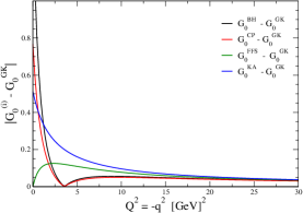
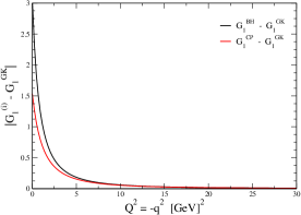
Figure 1: The differences among the electromagnetic form factor, $\delta G0$ and $\delta G_{1}$, given by the Inna Grach [61] prescription and other prescriptions in the literature [10] (KA),[62] (CP),[63] (BH) and [64] (FFS), the Eq.(21,22,23) and Eq’s.(24), above. Right, the differences for $G_{0}$ form factors, and left, $G_{1}$. If the zero mode, or non-valence contributions are include, the differences for all prescriptions are zero, because the differences are proportional to the angular condition, Eq.(14).

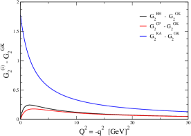
Figure 2: The differences for the quadrupole form factor $\delta G_{2}$, for the prescriptions present here is show in the figure above. The prescriptions given in the reference [64], have for the quadrupole rho meson form factor, the same expression in the reference [62], (see the Eqs. (21), (22), (23) and Eqs. (24)).

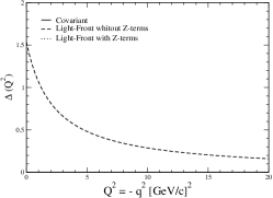
Figure 3: (Left), The zero of the charge form factor with the Eq. (25)), and, (right), the angular condition, $\Delta(Q^{2})$, each figure calculated with instant form and light-front approach. For both, calculations, the quark mass, is $m_{q}=0.430~{}GeV$ and $m_{R}=3.0~{}GeV$. In the figures above, if the z-terms, or zero modes is not include, the value of zero for Eq. (25), is different (about $2.4~{}GeV^{2}$), and also, the angular condition is not satisfied. The figure at left, show the angular condition, and, the strong breaking of the rotational symmetry, if the zero modes, or pair terms, is not taken in account.

For all prescriptions presented here, [61, 62, 63, 64], if the angular condition is satisfied, Eq. (13), follows immediately the expression below for the electromagnetic charge form factor, $G_{0}$:

$$G_{0}~{}=~{}\frac{1}{3}\left[~{}J^{+}_{xx}+2J^{+}_{yy}\right]~{}.$$ (25)

The equation above, produce the same charge electromagnetic form factor with the instant form basis calculations, and, is exactly the same for all prescriptions given above [20, 60]. Though, if the zero modes, or pair terms, are not included, the results with the instant form basis and light-front are not the same, and, need to add the zero modes or non-valence contributions to have the same results for both approaches.

The charge electromagnetic form factor for spin-1 particles, like the deuteron [67, 68], or rho meson [20, 21, 60, 69, 70], have a zero, i.e., $G_{0}(q^{2}_{zero})=0$. In order to see the zero position of the charge form factor ($G_{0}$), with the present light-front model, for the expression given above, Eq. (25), we show the Fig. (3), right, (this figure, is not normalized to 1), and, the zero for this sum appears when the moment transfer is about $\simeq 3.0~{}GeV^{2}$, and the inclusion of the zero modes; for another side, if the zero modes is not include, the position of this zero in the momentum transfer is different, $\simeq 2.4~{}GeV^{2}$ (see also the angular condition, in the Fig. (3), left). In order to keep the correct position of the charge electromagnetic form factor for spin-1 particles, is crucial include the non-valence contributions or zero-modes to the electromagnetic current for spin-1 particles.

In the discussions above, we have demonstrated, with the use of the relations given in the reference [26], ie., Eqs. (8), (9) and (10), for all prescriptions found in the literature with the light-front approach for spin-1 particles, given the same expression for the electromagnetic form factors, charge, magnetic and quadrupole. That procedure, is equivalent to take into account the zero modes, or, non-valence contributions to the electromagnetic current for the spin-1 particles [26]. In the last, the zero-mode, are very important to keep the full covariance with the light-front approach (see more in the references [21, 23, 30, 65, 66]).

Vector decay constant: Besides the electromagnetic form factors, also the electromagnetic decay constant of the rho meson was calculated with the present model [20]. We use the following expression to the decay constant for spin-1 particles [34],

$$\imath\epsilon_{\lambda}^{\mu}\sqrt{2}f_{\rho}=\langle 0|\bar{q}\gamma^{\mu}q|p\rangle~{}.$$ (26)

The expression for the decay constant with the considered model here, is given by the following expression,

$$f_{\rho}=\--\imath\frac{N_{c}N}{4(2\pi)^{4}}\int\frac{d^{2}k_{\perp}dk^{+}dk^{-}Tr\left[(\hbox to0.0pt{/\hss}{k}-\hbox to0.0pt{/\hss}{p}+m)\gamma^{+}(\hbox to0.0pt{/\hss}{k}+m)\,\epsilon_{z}\cdot\Gamma\right]\,\Lambda(k,p)}{k^{+}(p^{+}-k^{+})(k^{-}-k^{-}_{on}+\frac{\imath\epsilon}{k^{+}})(p^{-}-k^{-}-\frac{(p-k)_{\perp}+m^{2}}{p^{+}-k^{+}}+\frac{\imath\epsilon}{p^{+}-k^{+}})}~{},$$

where the polarization vector chosen is  $\epsilon^{+}_{z}=1$ and the vector particle it is in the rest frame, $p^{\mu}=(p^{0},\vec{0})$. After the Dirac trace performed and the $k^{-}$ integration done, result in:

$$f_{\rho}=\dfrac{N_{c}N}{m_{\rho}}\int\dfrac{d^{2}k_{\perp}dx}{(2\pi)^{3}}\dfrac{tr[\theta^{+}]}{x(1-x)^{3}(m^{2}_{\rho}-M^{2}_{0})(m^{2}_{\rho}-M^{2}_{R}(m_{R},m^{2}))^{2}}\ ,$$ (27)

where $tr[\theta^{+}]$, is the function defined below from Dirac trace in the expression above:

$$tr[\theta^{+}]=\left(-4k^{+2}+4k_{\perp}^{2}+4k^{+}P^{+}+4m^{2}\right)-\dfrac{m_{\rho}}{2}\dfrac{(2k^{+}-P^{+})(k_{on}^{-}-k^{+})4m}{\left(\dfrac{P^{+}k_{on}^{-}+P^{-}k^{+}}{2}+m_{\rho}m\right)}~{},$$ (28)

and with  $M_{R}^{2}(m^{2}_{a},m^{2}_{b})=\frac{k_{\perp}+m_{a}^{2}}{x}+\frac{k^{2}_{\perp}+m_{b}^{2}}{1-x}$,  $M_{0}=M^{2}(m^{2},m^{2})$ and $x=k^{+}/p^{+}$. The constant $N$, is found after the normalization condition for the charge electromagnetic form factor, $G_{0}(0)=1$. The function $\theta^{+}$, have two terms, a part without $k^{-}$ dependence and another with $k^{-}$ dependence. In refs. [20, 23, 24, 26], it was shown for the matrix elements of the electromagnetic current $J_{ji}^{+}$, with terms proportional a $k^{-}$, can lead to breaking of the rotational symmetry, but not necessarily; as in the case of the pi meson, where despite there being proportionately energy in the light-front, the contribution of pair terms or zero-modes vanish [23, 27]. For the case of the present work, the rho meson decay constant, calculated with the vertex, Eq. (1);  the second term, which could make a contribution, does not contribute, because the structure of the vertex used ref. [20]; but, for the ref. [42], the zero-modes terms survives, in virtue of the vertex structure utilized.

Table 1: $\rho$-meson low-energy electromagnetic observables calculate with the present light-front model, and compared with diferents models in the literature.

	$f_{\rho}$ [MeV]	$\mu~{}[e/2m_{\rho}]$	$Q_{d}~{}[e/m^{2}_{\rho}]$	$<r^{2}>~{}[fm^{2}]$
This work	153.66	2.10	-0.898	0.267
Pichowsky [48]	153.95	2.69	-0.055	0.61
Jaus [7]	-	1.83	-0.330	-
Aliev [9]	-	$2.4\pm 0.4$	$0.85\pm 0.15$	-
Biernat [17]	-	2.20	-0.47	-
Choi [21]	-	1.92	-0.430	-
Melikhov [31]	-	2.35	-0.364	-
Samsonov [36]	-	$2.00\pm 0.3$	-	-
Pitschmann [41]	-	2.11	-0.850	0.26
Krutov [44, 45]	152$\pm$8	2.16$\pm$0.03	-	0.56$\pm$0.04
Sun [46, 47]	-	2.06	-0.323	0.52
Hawes  [48]	-	2.69	-0.055	0.61
Cardarelli [60]	-	2.26	-0.367	0.35
Bhagwat [69]	-	2.01	-0.41	0.54
Roberts [70]	-	2.11	-0.85	0.31
Serrano [72]		2.57	-1.05	0.67
Gudiño [73]	-	2.1$\pm$0,5	-	-
Simonis [74]	-	2.06	-	-
Simonis [75]	-	2.17
Owen [50]		2.145	-0.733	0.670
Shultz [51]	-	2.17	-0.540	0.30
PDG [71]	153 $\pm$ 8	-	-	-

Results. The electromagnetic form factors, $G_{0},G_{1}$ and $G_{2}$ was calculated here with the vertex model $\rho-q\bar{q}$, Eq.(1), utilized previously in the reference [20]. Was already noted in previous works, the various prescriptions in the literature does not given the same results for the electromagnetic form factors, compared with the covariant impulse approximation [20, 22]. Because the dependence of which matrix element of the electromagnetic current is eliminate with the angular condition equation, [20, 61], we have some freedom in eliminate the matrix elements $I^{+}_{mm^{\prime}}$, but, if the matrix element $I^{+}_{00}$ is not eliminate, the rotational symmetry is broken [20, 22, 26], and, we have the zero modes, or, non-valence contributions. In the present work, after the use of the relations given in Eq.(10), all prescriptions found in the literature given the same results for the electromagnetic form factors [20, 26]. However, the prescription utilized by Inna Grach et al., [61], give exactly the same results, if compared with the covariant impulse approximation, for all observables calculated here, ie., the electromagnetic form factors,  $G_{0},G_{1},G_{2}$, electromagnetic radius and the rho meson decay constant.

With the constituent quark mass $m=m_{u}=m_{d}=0.430~{}GeV$, the regulator mass $m_{R}=3.0~{}GeV$ and the experimental rho mass, $m_{\rho}=~{}0.770~{}GeV$, we have obtained the value of the decay constant $f_{\rho}=154~{}MeV$, very close with the experimental data $153\pm 8~{}MeV$ [71]; the electromagnetic radius is $<r^{2}>=0.267~{}fm^{2}$, the magnetic moment $\mu=2.205~{}[e/2m_{\rho}]$,  and the quadrupole moment $Q_{d}=-0.0586~{}fm^{2}$, the values of the observables obtained here, are comparable with another’s models in the literature (see the table I).

In the Fig.4, we present the charge and magnetic form factors, $G_{0}$ and $G_{1}$, calculated with the parameters given above for various prescription in the literature.

The calculations present in the Fig. 4, are made without non-valence contributions, dashed lines and with add the non-valence contributions, solid lines. All calculation are compared with the covariant impulse approximation calculation, black solid line. It is seen in the figures for the electromagnetic form factors, the Inna Grach prescription [61], give the same result compared with the covariant impulse approximation. After the use of the relations Eqs. (9) and Eq. (10), which correspond in the end, to add the non-valence contributions to the matrix elements of the electromagnetic current, all the prescriptions given the same results, colors solid line.

In the Fig. 6, (left), the positions of the zeros for the charge electromagnetic form factor, is explored, and with the present model, the position of the zeros , are linear with the rho meson bound squared mass; or with other words, the behavior of the zero positions of the charge electromagnetic form factors is given by $q^{2}_{zero}\simeq 5m^{2}_{\rho}$, its proportional the meson spin-1 bound state mass (see the Fig. 6, the black solid line).

For the present work, the charge form factor zero appear around, $Q^{2}=3.0~{}GeV^{2}$ for the experimental rho meson mass $(770~{}MeV)$, (see the also the Fig. 4).  Recently, the reference [70], with Schwinger-Dyson approach, found $~{}5.0~{}GeV^{2}$. Late, the based Schwinger-Dyson calculation, [69], have that zero about, $3.8~{}GeV^{2}$. The ”universal ratios” [43, 63], for the charge form factor, with the experimental mass for rho meson, $m_{\rho}=0.770~{}GeV$, give for the zero, $q^{2}_{zero}\approx 3.6~{}GeV^{2}$, which is not far from the value predicted in this model.

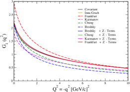
Figure 4: Charge form factor (left) and magnetic form factor (right) for the rho meson. The quark mass are $m_{u}=m_{\bar{d}}=0.430$ GeV, for the regulator mass $m_{R}=3.0$ GeV, calculated with various prescriptions in the literature [10, 61, 62, 63, 64].

.

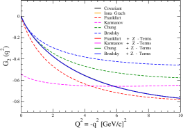
Figure 5: Quadrupole $G_{2}(q^{2})$ electromagnetic form factor, labels is the same from the Fig.4

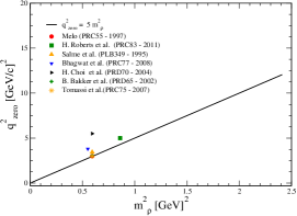
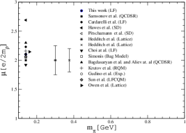
Figure 6: (Left) Charge electromagnetic form factor zero, $G_{0}(q^{2}_{zero})=0$ in function of the rho meson mass, in the present model and compared with another’s models in the literature. (Right) Magnetic moment for the rho meson compared with another models in the literature,  (QCDSR) QCD sum rules, (LF) Light-Front approach, (SD) Schwinger-Dyson, Lattice calculations, Bag model, including with some experimental analysis.

The magnetic momentum calculated in the present work, is compared with others model from the literature in the Fig. 6 (right), in function of the pion mass, because in the same figure, the results from Lattice calculations are show [49].

In the light-front approach, besides de valence components, we have non-valence contributions to the matrix elements of the electromagnetic current [20, 22, 23, 24, 30, 42]. However, in the present work, independent of the prescription used to extract the electromagnetic form factors and thus calculating some observables, such as the decay constant, electromagnetic radius, magnetic and quadrupole momentum, we have obtained the same results; for this, the relations between the matrix elements of the electromagnetic current at level of Dirac structure are fundamental, Eq. (10) [26]. With that relations, we arrival in Eqs. (17), (18) and, (20), it is exactly the same equations utilized in the Inna prescription [61], in order to obtain the electromagnetic form factors for spin-1 particles, in case here, the rho meson. Also, with the Eq.(25), the charge electromagnetic form factor, calculated in the instant form basis, not have any dependence with prescriptions, but, if calculated, with the light-front approach, the rotational symmetry is broken, and, after add the zero modes to the matrix elements of the electromagnetic current, the rotational symmetry is completely restored. The position of the zero for the charge electromagnetic form factor before the addition of the zero modes is around  $2.5~{}GeV^{2}$, after added zero modes, is around $3.0~{}GeV^{2}$, the same with the instant form basis calculations, (see in the Fig. 4, right panel).

Concluding, the present work, extends the previous works,  [20, 26], for spin-1 particles with a light-front constituent quark model, and show an unambiguous procedure to extract the electromagnetic form factor of the plus component of the electromagnetic current, free of the zero modes or pair terms contributions to the matrix elements of the electromagnetic current.

A study of others components the electromagnetic current in order to extract electromagnetic form factors for particles of spin-1, and calculate the observables, it is in progress.

Acknowledgements. This work was partially supported by the Fundação de Amparo à Pesquisa do Estado de São Paulo, FAPESP, Brazil, Process
No.2015/16295-5, and FAPESP Temático,Brazil,Process No.2017/05660-0.
Conselho Nacional de Desenvolvimento Científico e Tecnológico (CNPq), Brazil, grants Nos. 308025/2015-6 and 401322/2014-9. This work is part of the project INCT-FNA Proc. No. 464898/2014-5.

References

[1]
S. J. Brodsky, H.-C. Pauli, and S. S. Pinsky,
Phys. Rep. 301 (1998) 299.
[2] P. Maris and P. C. Tandy,
Phys. Rev. C 60 (1999) 055214.
[3] C. D. Roberts and A. G. Willians,
Prog. Part. Nucl. Phys. 33 (1994) 477.
[4] C. D. Roberts and S. M. Schmidt,
Prog. Part. Nucl. Phys. 45 (2000) S1.
[5] V. Braguta and A. I. Onishchenko,
Phys. Lett. B 591 (2004) 267.
[6] V. V. Braguta and A. I. Onishchenko,
Phys. Rev. D 70 (2004) 033001.
[7] W. Jaus,
Phys. Rev. D 67 (2003) 094010.
[8]
T. M. Aliev and M. Savci,
Phys. Rev. D 70 (2004) 094007.
[9] T. M. Aliev, A. Özpineci and M. Savci,
Phys. Lett. B 678 (2009) 470.
[10]V. A. Karmanov,
Nucl. Phys. A 608 (1996) 316.
[11] V. Braguta, W. Lucha and D. Melikhov,
Phys. Lett. B 661 (2008) 354.
[13] S. J. Brodsky and G. F. de Téramond,
Phys. Rev. D 77 (2008) 056007.
[14] J. Bijnens, P. Gosdzinky and P. Talavera,
Phys. Lett. B 429 (1998) 111.
[15] O. Leitner, J.-F. Mathiot, N. A. Tsirova,
Eur. Phys. J. A 47 (2011) 17.
[16] V. A. Karmanov, J.-F. Mathiot and V. A. Sminorv,
Phys. Rev. D 75 (2007) 045012.
[17]E. P. Biernat and W. Schweiger,
Phys. Rev. C 89 (2014) 055205.
[18]
R. J. Perry, A. Harindranath, and K. G. Wilson,
Phys. Rev. Lett. 65 (1990) 2959.
[19] S. J. Brodsky, J. R. Hiller,
D. S. Hwang and V. A.Karmanov, Phys. Rev. D 69 (2004) 076001.
[20]J. P. B. C. de Melo and T. Frederico,
Phys. Rev. C 55 (1997) 2043.
[21] H.-M. Choi and C. R. Ji,
Phys. Rev. D 70 (2004) 053015.
[22] B. L. G. Bakker and
C. R. Ji, Phys. Rev. D 65 (2002) 116001.
[23]J. P. B. C. de Melo, H. W. L. Naus,
and T. Frederico, Phys. Rev. C 59 (1999) 2278.
[24]J. P. B. C. de Melo, H. W. L. Naus,
T. Frederico and P. U. Sauer, Nucl. Phys. A 660 (1999) 219.
[25]
Y. Li, P. Maris and J. Vary,
Phys. Rev. D 97 (2018) no.5, 054034.
[26]
J. P. B. C. de Melo and T. Frederico, Phys. Lett. B 708 (2012) 87.
[27]
E. O. da Silva, J. P. B. C. de Melo, B. El-Bennich and V. S. Filho,
Phys. Rev. C 86, 038202 (2012) 038202.
[28] P. Maris, C. D. Roberts, Phys. Rev. C 56 (1997) 3369.
[29]F. P. Pereira, J. P. B. C. de Melo, T. Frederico,
L. Tomio, Nucl. Phys. A 610 (2007) 610.
[30] J. P. B. C. de Melo,
T. Frederico, E. Pace and G. Salmè,
Nucl. Phys. A 707 (2002) 399; ibid. Braz. J. Phys. 33 (2003) 301.
[31] D. Melikhov and S. Simula,
Phys. Rev. D 65 (2002) 094043.
[32]G. H. Yabusaki, I. Ahmed, A. Paracha,
J. P. B. C. de Melo and B. Bennich,
Phys. Rev. D 92, (2015) 034017.
[33]
C. Fanelli, E. Pace, G. Romanelli, G. Salme and M. Salmistraro,
Eur. Phys. J. C 76 no. 5, (2016) 253.
[34]
J. P. B. C. de Melo, T. Frederico, E. Pace and G. Salmè,
Phys. Lett. B 581 (2004) 75; ibid. Phys. Rev. D 73 (2006) 074013.
[35]
C. Adamuscin, G. I. Gakh and E. Tomasi-Gustafsson,
Phys. Rev. C 75 (2007) 065202; A. Dbeyssi, E. Tomasi-Gustafsson, G. I. Gakh and C. Adamuscin,
Phys. Rev. C 85 (2012) 048201.
[36] A. Samsonov, JHEP 0312 (2003) 061.
[37] H. R. Grigoryan, Phys. Lett. B 662 (2008) 158.
[38]T. M. Aliev, A. Ozpineci and M. Savci,
Phys. Lett. B 678 (2009) 470.
[39]
D. Garcia Gudino and G. Toledo Sanchez,
Phys. Rev. D 81 (2010) 073006.
[40]
H. M. Choi and C. R. Ji, Phys. Lett. B 696 (2011) 518.
[41] M. Pitschmann, C.-Y. Seng,
M. J. Ramsey-Musolf, C. D. Roberts, S. M. Schmidt, D. J. Wilson,
Phys. Rev. C 87 (2013) 015205.
[42]
H. M. Choi and C. R. Ji, Phys. Rev. D 89 (2014) 033011.
[43] J. P. B. C. de Melo, C. R. Ji and T. Frederico,
Phys. Lett. B 763, (2016) 87.
[44]
A. F. Krutov, R. G. Polezhaev and V. E. Troitsky,
Phys. Rev. D 93, (2016) 036007.
[45]
A. F. Krutov, R. G. Polezhaev and V. E. Troitsky,
Phys. Rev. D 97, (2018) 033007.
[46]B. D. Sun and Y. B. Dong,
Phys. Rev. D 96 (2017) 036019.
[47]
B. d. Sun and Y. b. Dong,
Chin. Phys. C 41 (2017) 013102.
[48]
F. T. Hawes and M. A. Pichowsky,
Phys. Rev. C 59 (1999) 1743.
[49]
J. N. Hedditch, W. Kamleh, B. G. Lasscock, D. B. Leinweber, A. G. Williams and J. M. Zanotti,
Phys. Rev. D 75 (2007) 094504.
[50]
B. Owen, W. Kamleh, D. Leinweber, B. Menadue and S. Mahbub,
Phys. Rev. D 91 074503 (2015).
[51]
C. J. Shultz, J. J. Dudek and R. G. Edwards,
Phys. Rev. D 91 (2015) 114501.
[52]
P. G. Blunden and G. A. Miller,
Phys. Rev. C 54 (1996) 359. doi:10.1103/PhysRevC.54.359.
[53]
P. G. Blunden, M. Burkardt and G. A. Miller,
Phys. Rev. C 60 (1999) 055211.
[54]
G. M. Huber, G. J. Lolos and Z. Papandreou,
Phys. Rev. Lett. 80 (1998) 5285.
[55]
G. M. Huber et al. [TAGX Collaboration],
Phys. Rev. C 68 (2003) 065202.
[56]
J. P. B. C. de Melo, K. Tsushima, B. El-Bennich, E. Rojas and T. Frederico,
Phys. Rev. C 90 (2014) 035201.
[57]
J. P. B. C. de Melo, K. Tsushima and I. Ahmed,
Phys. Lett. B 766 (2017) 125.
[58]
W. R. B. de Aráujo, J. P. B. C. de Melo and K. Tsushima,
Nucl. Phys. A 970 (2018) 325.
[59]
J. P. B. C. de Melo and K. Tsushima,
(To appear Phys.Lett. B), arXiv:1802.06096 [hep-ph].
[60]
F. Cardarelli, I. L. Grach, I. M. Narodetsky,
G. Salmè, S. Simula, Phys. Lett. B 349 (1995) 393.
[61] I. L. Grach and L. A. Kondratyuk, Sov. J. Nucl. Phys. 38 (1984) 198;
I. L. Grach, L. A. Kondratyuk, and M. Strikman, Phys. Rev. Lett. 62 (1989) 387.
[62]
P. L. Chung, W. N. Polyzou, F. Coester and B. D. Keister, Phys. Rev. C 37 (1988) 2000.
[63] S. J. Brodsky and J. Hiller, Phys. Rev. D 46 (1992) 2141.
[64] L. L. Frankfurt, T. Frederico, and M. Strikman,
Phys. Rev. C 48
(1993) 2182.
[65] J. P. B. C. de Melo and T. Frederico, Braz. J. Phys. 34 (2004) 881.
[66] J. P. B. C. de Melo, J. H. O. Sales,
T. Frederico, and P. U. Sauer, Nucl. Phys. A 631 (1998) 574c.
[67] M. Garcon and J. W. Van Orden,
Adv. Nucl. Phys. 26 (2001) 293.
[68] R. A. Gilman and F. Gross,
J. Phys. G 28 (2002) R37.
[69] M. S. Bhagwat and P. Maris, Phys. Rev. C 77 (2008) 025203.
[70]
H. L. L. Roberts, A. Bashir, L. X. Gutierrez-Guerrero, C. D. Roberts and D. J. Wilson,
Phys. Rev. C 83 (2011) 065206.
[71] The Review of Particle Physics (2018),
M. Tanabashi et al. (Particle Data Group), Phys. Rev. D 98 (2018) 030001.
[72]
M. E. Carrillo-Serrano, W. Bentz, I. C. Cloët and A. W. Thomas,
Phys. Rev. C 92 (2015) 015212.
[73] D. García Gudiño and G. Toledo Sánchez,
Int. J. Mod. Phys. A 30 (2015) 1550114.
ibid., Int. J. Mod. Phys. Conf. Ser. 35 (2014) 1460463.